The Role of Education in the IT diffusion: Evidence from the British Household Panel Survey 1 . By Luis Hernandez 2 University of Essex Department of Economics Abstract We analyse the importance of education as a measure of human capital in the computer and Internet diffusion within households in the UK for the period from 2000 to 2005. We employ data from the British Household Panel Survey (BHPS) and we use a modified version of a dynamic random effect probit model proposed by Cappellari and Jenkins (2009) and a propensity matching score technique proposed by Rubinstein and Rubin (1983) to measure the importance of education in the IT diffusion among households. Our results suggest that higher levels of education at home have played an important role in the spread of these technologies and that these technologies tend to create a habit among users which is stronger for more educated families. 1 Please do not cite unless authorization from the author. If you want to contact me, please do to my email account: [email protected]2 This is a preliminary work from my PhD thesis. I acknowledge the support of my sponsors in my PhD studies: The Alßan Programme of the European Union (scholarship No. E07D400759GT) and the Department of Economics of the University of Essex, and also I appreciate the helpful comments and suggestions of Kate Rockett, Pierre Regibeau , Joao Santos da Silva and the ones received from Alison Booth and colleagues participating in the RSS seminar from the University of Essex. 1
Transcript
The Role of Education in the IT diffusion: Evidence from the British
Household Panel Survey1.
By Luis Hernandez2
University of Essex
Department of Economics
Abstract
We analyse the importance of education as a measure of human capital in the
computer and Internet diffusion within households in the UK for the period from 2000
to 2005. We employ data from the British Household Panel Survey (BHPS) and we
use a modified version of a dynamic random effect probit model proposed by
Cappellari and Jenkins (2009) and a propensity matching score technique proposed by
Rubinstein and Rubin (1983) to measure the importance of education in the IT
diffusion among households. Our results suggest that higher levels of education at
home have played an important role in the spread of these technologies and that these
technologies tend to create a habit among users which is stronger for more educated
families.
1 Please do not cite unless authorization from the author. If you want to contact me, please do to my email account: [email protected] is a preliminary work from my PhD thesis. I acknowledge the support of my sponsors in my PhD studies: The Alßan Programme of the European Union (scholarship No. E07D400759GT) and the Department of Economics of the University of Essex, and also I appreciate the helpful comments and suggestions of Kate Rockett, Pierre Regibeau , Joao Santos da Silva and the ones received from Alison Booth and colleagues participating in the RSS seminar from the University of Essex.
1
1. Introduction
The spread of knowledge, the reduction of uncertainty and the increase of
opportunities are considered to be important elements for economic growth and
development. With the invention of the Internet a couple of decades ago, a new tool to
enhance the performance of these elements was created, and because of this policy
makers have been keen to improve access to this technology for all individuals.
Since the 90s, the Internet has been diffusing rapidly worldwide, but despite this swift
diffusion, developing economies are not adopting it as quickly as developed ones,
which has created a gap that appears not to close and is known as the “digital divide”.
This is a matter of concern for policy makers because it appears that the potential
benefits of the Internet use are not going to reach all individuals. Recent figures from
2009 indicate that the proportion of Internet users in developed nations were around
68 per 100 inhabitants whilst this figure was only about 18 percent for developing
countries (Information Telecommunication Unit from United Nations).
The Internet is designed to exchange information between networks of
computers, and because the most common way to access the Internet is with a
computer, access to this technology is also important for the Internet diffusion.
Because computers appear to be skill biased technologies in the sense that countries
with better educational attainment by its inhabitants are better adopters of these
technologies than less educated ones (Caselli and Coleman II 2001), it is not
surprising to find research in which the Internet is also considered to be a skill biased
technology (see, for example, Chinn and Fairlie 2007).
The Internet and computers are Information Technologies (or IT for short)
which have been adopted not only quickly but widely by a cross section of economic
actors in all countries of the world (e.g. individuals, firms, schools, governments), and
what they all have in common is that they are conformed by individuals living in
households; therefore, a good measure of the capacity of a country to adopt IT goods
is the proportion of households that are IT users.
According to the OECD (2001) education and income appear to be among the
main factors that influence a household’s IT decision. Other factors that affect a
household’s decision are household type, size, race, age, gender, language and
location. Because developed economies tend to be richer, more educated and have
better services than developing ones, we can infer that if education is relevant for the
IT adoption in households in a developed economy, it is also going to be play an
2
important role for the diffusion of IT goods in a developing one. Lack of educative
skills is a barrier for illiterate or low educated individuals and families in using IT
technologies and so benefitting from their use, but in developed economies, where the
proportion of low educated individuals tend to be low, higher education might still
have an important role to play not only in the adoption but in the speeding up of the
diffusion of IT goods. The role of habits are also important in deciding whether those
that are users subsequently remain as users of a technology (Becker 1992) but we still
have no information about the role of education and other determinants in the decision
of current users to continue as users or to stop using IT goods once they have been
adopters. Most studies have assumed that the adoption is an absorbent state in which
once a consumer becomes an IT user, they remain in that state. Therefore research has
applied static models either using panels or cross-sectional analysis because it has not
checked the previous state in the consumption, which might be important for
development of a habit or an addiction in IT use, and also they have not taken into
account for unobserved characteristics such as unobserved heterogeneity that might
affect a households’ decision not only to adopt these technologies but also to remain
as a user (see for example Robertson, Soopramanien, and Fildes 2007; Flamm and
Chaudhuri 2007a; Flamm and Chaudhuri 2007b; Chaudhuri, Flamm, and Horrigan
2005; Andres et al. 2007).
Hence in this paper we want to address the following questions in a developed
economy context: What is the role of the educational attainment of households in the
IT diffusion? What would be the diffusion pattern if all households had all high or all
low educational attainment?, and how much does high-education affect the speed of
the diffusion among households that are more educated?. To answer the first two
questions we use a version of a multivariate dynamic probit panel model proposed by
Wooldridge (2005) and modified by Cappellari and Jenkins (2009), and for the last
we use a propensity matching score technique proposed originally by Rosenbaum and
Rubin (1983).
For this paper we use data from the British Household Panel Survey (BHPS)
for the period 2000-2005. The United Kingdom is a highly developed human capital
country, ranked 21st in the world (see Human Development Report (2009) from
United Nations), with nearly 100 percent adult literacy rate and a combined gross
enrolment ratio in 2007 of 89.2 percent of primary, secondary and tertiary education
gross enrolment ratios which illustrates that this is a country in which most of the
3
inhabitants have the opportunity and economic means to achieve a high educational
qualification and develop the skills necessary to use IT goods. About the IT use,
according to estimates from the Information Telecommunication Union, around 84
out of 100 inhabitants were Internet users in the UK in 2009 (either at home or outside
it), which makes an interesting country to study the IT diffusion to find if there is
evidence of its importance of education in the IT diffusion within households over
time.
According to official estimates (Office for National Statistics (ONS) 2007)
household access to the Internet at home during the last quarter of 2000 was around
34 percent and at the end of the last quarter of 2004 it was 52 percent, which is an
average annual increase of 4.2 percentage points (pps) in new households during this
period this being close to the average we observe in our sample.3
According to the ONS (2007), the home is the most common place for
individuals to go online and the most common way to go online is with a computer.
The main reasons why UK households subscribed to the Internet service at home were
for access to more information (46 percent), communication (28 percent), to be
technical updated (22 per cent) and for their children (20 percent). According to their
data, households that are IT users tend to have higher educational qualifications, more
income, and dependent children, and the adults who currently use the internet tend to
be younger. As far I am aware, and surprisingly, there has been no research on IT
diffusion among households using a dynamic model, or adopting the approach
proposed by Cappellari and Jenkins (2009). Analysing this process it would overcome
the drawback of not having observed the household since it adopted for first time the
Internet and computers,, which could be useful for applying a survival analysis
method.
This paper focuses on finding the main characteristics that contribute to the
dynamics of the diffusion of IT goods among UK households and to identify the
importance played by educational attainment, as a measure of the human capital of
households. This paper is organized as follows: part 2 presents the data and some
figures about the observed trend in the IT diffusion among UK households, part 3
presents the methodological framework, part 4 our empirical findings, and the last
part, we present our conclusions and final remarks.
and this can be estimated using a standard random effect Probit model. The approach
of Cappellari and Jenkins, modifies equation (1) by first proposing instead of using
current covariates with the outcome variable, using the lag of them 1, −tiX and
secondly, adding a set of interaction terms of the set of covariates 1, −tiW (that could be
a subset of 1, −tiX ) with the lag of the outcome variable 1, −tiy . Hence equation (3) can be
expressed as:
7
{ }Tt
ZyyyXXcXyyP
iiititititi
iittiit
,...2,1)*(
),,|1(
0101,21,1,11,
11,
=++++++Φ
==
−−−−
−−
υγααρββ , (4)
In this expression we assume that 1,1, −− = titi XW . We estimate the parameters of this
equation using a standard random effect probit model (4) and we also include in the
list of covariates, trend and regional dummies.
The addition of the iteration terms allows each variable to have a different
effect on the entry, persistence and exit rates of each state.
The entry rate or probability of adopting a computer in the current period by a
household is the conditional probability of adopting a computer (or the Internet) when
this household was not a user of it the year before 01, =−tiy , that is
)(),,0|1(
01011,
,011,
iiiti
iiittiitit
ZyXZyXyyPe
υγααβ ++++Φ====
−
−−(5)
A positive coefficient of a variable in (5) results in the positive effect of an
increase in this variable over the entry rates.
The persistence rate or probability of a household remaining a computer (or
Internet) user in the current period given that the previous year this household was a
user 11, =−tiy is
TtZyX
ZyXyyPs
iiiti
iiittiitit
,...2,1))((
),,,1|1(
010211,
,011,
=++++++Φ
====
−
−−
υγααρββ (6)
and hence the exit rates for households at risk (those that were users the previous year
11, =−tiy ) is then itit se −= 1 . A positive coefficient of a variable in (6) of the terms
with no interaction implies a positive effect in the change of this variable over
persistence rates (and a negative one in the exit rates), and for the variables that have
interaction terms, we have that the sign of the sum of both coefficients of a variable
indicates the direction of the change of the persistence rates (and vice versa for exit
rates) due to a change in this variable.
This model proposed by Cappellari and Jenkins represents a first order
Markov process because the dynamics are of first order and it also allows the
covariates to have a different effect on the entry, persistence and exit rates.
8
Propensity Score Matching
It is well known that comparing the outcome of one group that has been
exposed to a treatment and another that has not, gives an estimate that is biased
towards the effect of the treatment on the treated unless the process of assignment of
the treatment status for each individual was random; on this case, treated units are
similar to non treated and hence, the propensity score method proposed by
Rosenbaum and Rubin (1983) is a technique used to remove the bias due to observed
covariates.
If the treatment assignment is an independent conditional on a set of a
covariates, the treatment assignment is an independent conditional on a scalar
function called the propensity score, then comparing the average outcome of treated
units with non treated ones that have a similar score, it gives us an estimate of the
average treatment effect on the treated units. The propensity score is then the
probability of being treated given an observed set of covariates iX .
This technique has been used widely in different sorts of problems such as the
evaluation of training programmes or social influences on the development of
individual habits. For example, this has been applied to assess the effect of training in
employment outcomes by Dehejia and Wahba (1998) to show that this technique can
give similar results to those found by Lalonde (1986) in a randomized experiment,
this being the gold standard, or by Francesconi, Jenkins and Siedler (2009) which
estimated the effect of growing up in a family headed by a lone mother on the
smoking habits of young individuals.
Formally, if the outcome is independent of the treatment conditional on a set
of covariates, the outcome is independent of a scalar function of a set of covariates
known as the propensity score )|1Pr()( iii XDXp =≡ . To apply this method, first the
score is estimated using a probit or logit model and then the estimate of average
treatment effect on the treated is found by comparing treated units in the treatment
group { }1| == iDiT with those of the control with a similar score or constructing a
comparison unit using a weighting scheme. In our case we construct the comparison
outcome for each unit Ti ∈ , iy , using a Kernel-based Matching method. Following
Sianesi (2001) we use all the units of the control group { }0| == jDjC and then the
9
comparison outcome for unit Ti ∈ is constructed using its score and the weighted
score of all comparison units, that is
∑
∑
∈
∈
−
−
=
Cj
ji
jCj
ji
i
hXpXp
K
yh
XpXpK
y)()(
*)()(
ˆ (7)
where K is the kernel distribution function, and h is the band width that is set to
penalise more those observations that in probability are far away from the score of the
unit i and weights more the ones that are closer to it. Then the average effect of the
treatment on the treated (ATT) is given by
∑=∈
= −=∆1
1 )ˆ(1|ˆDi
iiT yyN (8)
where N is the total number of elements in .T
4. Findings
4. 1 Dynamic model and counterfactual simulations
The results of the estimates of the households’ computer decision are shown in
table 1, and those for the Internet one are shown in table 2.
For each regression shown, the first column shows the coefficients of the
covariates without interaction, and the second shows the estimates of the variables
that have an interaction term with the lag of the dependant variable. The first column
shows the estimates associated with the entry rates, and the sum of the coefficients of
both columns of a variable is associated with the persistence rate or habit to remain as
a user. When there is no coefficient for a variable in the second column (no
interaction of this covariate with the lag of the dependent variable), the change in
entry rates and persistence rates due to a change of this variable has the same direction
as the sign of the estimate shown in the first column. The estimate of the lag of the
dependent variable is useful only to estimate the persistence rate, but not the entry
rate.
The mean longitudinal values of the covariates and the initial condition that
are used to explain the unobserved heterogeneity term are shown in the lower part of
the table together with the lag of the dependent variable and the estimate of the natural
logarithm of the variance of the unobserved heterogeneity term.
10
In this dynamic setup, households at risk of becoming a computer/Internet user
are those that do not have the technology in the previous period, and households at
risk of persisting as users are those that have that technology during the previous
period.
Households’ Computer decision
For the computer decision estimates shown in table 1, we explain first the
variables that have an interaction term with the lag of the dependent variable (which
might have a different effect on the entry and persistence rates), and then we explain
those variables that are associated with unobserved heterogeneity and the lag of the
dependent variable alone and the trend variables. The regional dummy variables,
although included, are not shown for brevity.
The variables that are related with the unobserved individual heterogeneity
affect the entry and persistence rates in the same direction; that is an increase in one
of this variable when its coefficient is positive will increase the idiosyncratic term and
therefore will increase the entry and persistence rates, and will decrease these rates
otherwise. The lag of the dependent variable affects only the persistence rate through
the lag term alone and its interaction with the dependent variables.
For the entry rates, for households at risk of becoming computer adopters, having
higher levels of education at home increases the probability of a household becoming
an adopter. The higher the educative level at home, the higher the predicted
probability to get a computer, as can be seen because the high education variable
estimate (0.59) is highly significative and positive and around twice that for the
medium education variable (0.29). The higher the family income, the presence of
children older than 5, especially those between 5 and 11 and over 15, improves the
probability of adopting a computer. For those households where the head is 50 or
more years old, or when the number of members older than pensionable age is higher,
the probability of adopting a computer becomes lower. The rest of the variables
having an interaction term (like living in own house) are not significative.
For the persistence rates, we focus on households that are already computer
users. For these, having a higher educative level increases the probability of staying as
users in the next period. For the high educated variable the coefficient of both
columns are significative and the sum of them is positive and equal to 0.33 (=0.59-
0.26) which is more than double the sum of the medium educative level 0.14 (=0.29-
0.15). This implies that more educated households are more likely to develop a
11
stronger habit that less educated ones. Although households with more income are
less likely to remain as computer users, the sum of the coefficients (-0.0003) is
smaller than the coefficient to adopt (0.0005), which indicates that income is more
important for the adoption decision than for the decision to exit once a household has
become a computer user.
When the head is white, the sum of coefficients that are significative4 is 0.57
which implies that this type of household is more likely to remain as a user after
becoming an adopter. Similarly when the head is in their 40s, the sum of significative
coefficients is positive (0.43) which implies that the probability of staying is larger for
them. Interestingly, when the head is 50 years old or older, despite it being more
difficult for this type of households to become adopters, they are more likely to
remain as users, which can be seen in the sum of the coefficients is about 0.19 (=0.61-
0.42). The presence of children over 5, especially when they are between 12 and 15
years old, improves the probability that a household continues to use a computer.
For households in which the head lives alone, the head is female, and/or there is a
greater number of members at home over pensionable age, they tend to be less likely
to remain as users after they have become adopters. The other variables with
interaction with the lag of the dependent variable not mentioned (such as the age of
the head is in the 30s) are not relevant for the households’ decision to stay as users in
the next period.
The estimate of the computer lag with no interaction is 1.04 and is highly
significative, which implies that there is a strong habit that is not captured by the
interaction with the other variables previously explained and which might be down to
the fact that computers are durable goods. As we explained above all the variables that
have an interaction term and increase the persistence rates are related to the
development of a habit. Some, such as the presence of children, might also reflect
further needs from computers for educational requirements and homework at home.
Over time, there is an increase in the probability that households at risk adopt a
computer, and for those that are users to remain in that state, and this is reflected by
the highly significative year dummies which increase from 0.16 in 2001 to 0.48 in
2004.
4 Only the coefficient of the second column (0.57), the one associated with the iteration term, appears to be significant for this variable.
12
For the unobserved heterogeneity term, which can measure the ‘ability of
household’ members or their tastes, the higher value of this variable implies not only a
higher adoption but also a higher incidence of staying. Table 1 shows that for higher
values of the longitudinal averages variables during our window: Living in own
house, family types: couple, lone parent, type of job of the head (managerial or a
skilled work), and the initial condition: had a computer in the initial year (2000), this
household tend to have a higher level of ‘ability’ or unobserved heterogeneity that
contributes to the decision to adopt and to remain as computer users. The positive
coefficient of the initial condition highlights that for those households that were
initially users in 2000, the unobserved heterogeneity is estimated to be higher.
The estimate of the variance of the unobserved ability is significative and equal to
0.28, which implies that 22 percent of the unexplained variation (0.28/1.28) in
adopting a computer is attributed to the unobserved individual heterogeneity.
Households’ Internet decision
For the Internet decision, we use the same variables as for the computer
dynamic model previously estimated but the lag and initial condition correspond to
the Internet variable, and, as before, the data covers the period 2000-2005. For the
first specification, we restrict our sample to those households (2227) that had a
computer during the 90s, and for the rest of regressions (2 to 4) we include all the
households in our samples (4236) that have had observations on Internet access over
consecutive periods. Results in (3) include covariate computer use in the initial year
(2000), and the estimates in (4) also include the computer access at home during the
previous year (t-1). The outcome variable of Internet access is measured in year t.
The computer variable access was introduced in specifications (4) to see if the
covariates that are significant for the computer access reduce its significance when we
introduce this variable, which, if that is the case, would suggest that they are relevant
only for the computer decision but not for that of the Internet and this is not the case,
as we explain below.
Here, households at risk to adopt the Internet are those that do not have a
computer, or those that have a computer but are not Internet users in the previous
year. Hence those at risk of adopting the computer are a subset of those at risk of
adopting the Internet. Those who decide to stay as Internet users in the next period
are those that have a computer and have had the Internet in the previous period,
13
therefore those at risk of remaining as Internet users are a subset of those at risk of
staying as computer users.
For the explanation of the table 2, for reasons of simplicity and brevity, we
focus on explaining the last regression (4), where the coefficients of interest tend to be
less biased, more efficient and not so different from those of the previous regressions
results (1 to 3). After we introduce the lag variable of computer use, the estimates of
the variables for the Internet decision do not vary much, especially the ones of more
interest to us: educational attainment variables, which suggest that they are still
relevant for the Internet decision even when a household has a computer but no
Internet.
For the entry rates, more educated households that are at risk of becoming
Internet users are more likely to become Internet adopters than less educated ones.
The coefficients of medium and high educational achievement at home are 0.29 and
0.50 respectively, and both are highly significative which reflects that there is also a
gradient of education over the Internet decision, even for households that have a
computer already. Households with higher levels of family income and have children
at home aged between 5 and 15 years old, especially those between 12 and 15, have a
higher likelihood of adopting the Internet. When the age of the head is over 40,
especially when he (she) is older than 50, or when she is female, the household has a
lower probability of becoming an Internet user than if this were not the case.
For those who are already Internet users, the probability of remaining as a user
is higher for a household that is more educated, which can be seen in the sum of the
coefficients that are significative for each educational variable are positive. . For the
high education variable, the sum of both coefficients is 0.27 and for the medium
educated households only the first coefficient is significative and is about 0.29.
Similarly, for the computer case, when the head is in his (her) 40s or over 50 years
old, despite the fact that being older does not favour the household decision to adopt
the Internet, once this household is an Internet user, it is more likely to remain as a
user for this unit and this is seen in the sum of both coefficients associated with each
variable; these being 0.12 and 0.11 respectively. The sum of the coefficients of the
income variable are negative (-0.0003) which implies that households with higher
levels of income are less likely to remain as Internet users. For households where the
head is female, or the partner lives alone, they are less likely to stay as Internet users.
14
Similar to the computer case, there is an increase over time in the probability of a
household at risk of adopting the Internet, and for those that are users to stay with that
technology for the next period, as reflected by the highly significative year dummies
which increase from 0.16 in 2001 to 0.45 in 2004.
For the unobserved individual effect, a higher value of this variable implies a
higher rate of Internet adoption and of persistence for those households at risk, i.e.
faster diffusion. For the Internet an increase in the longitudinal average value of the
following variables : family income, the head being single or family types: couples or
lone parent, or type of job of the head (Managerial or skilled), and the initial
conditions: having a computer in the year 2000 and the Internet in the year 2000,
increases the unobserved heterogeneity or ‘ability’ and therefore increases the entry
and persistence rates. Households with higher number of pensionable ages tend to
have lower unobserved heterogeneity term which affects negatively the diffusion of
the Internet.
Having a computer the previous year (t-1), increases the probability of
adopting the Internet in the current period (t) for those that are non Internet users, and
having Internet at home in the previous period has a bigger effect on the probability of
having the Internet current period than having only a computer, as can be seen with
the coefficient of the Internet user variable being 1.21 as compared with only having a
computer at 0.49.
The estimate of the variance of the individual effect is 0.36, which is highly
significative and accounts for 26.6 percent (0.36/1.36) of the total variance.
Because having the Internet in the previous period influences the decision of a
household to continue as a user, we found that there is evidence to suggest that use of
the Internet creates a habit especially for families that are more educated, have
children aged between 5-15, and where the head is older than 40, but it is less habitual
when the head is female or the family type is lone parent.
The persistence rates tend to be much higher than the entry rates which implies
that more and more households are becoming IT adopters and that they tend to remain
as users over time. Figures 2a and 2b show the predicted and observed entry rates of
our sample for households at risk of becoming computer and Internet users
respectively. We observe that for the computer entry rates, the observed rate is
between 12.6 and 13.4 percent in the period 2001-2005, whilst that for the predicted
one is between about 11 percent in 2001 and up to 15.2 in 2005.
15
<Figures 2a and 2b come here>
The observed Internet entry rates are between 12.9 in 2001 and 11.6 percent in
2005, while the predicted ones vary between 11.3 in 2001 and about 14 percent in
2005.
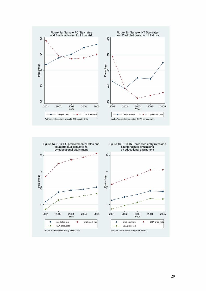
Figures 3a and 3b show the predicted and observed persistence rates for
households likely to stay as computer and Internet users, respectively. From these
graphs, we observe that the proportion of users that decide to stay is high (more than
90 percent) and tends to increase over time. For the stay rates of computer use, we
observe that the percent of households that remain as computers users in the current
period increases from 94.3 percent in 2001 to 95.6 percent in 2005, and the predicted
rate decreases from 95.9 percent in 2000 to 94.8 in 2003 and then increases slightly
again to around 95 percent in 2005. The stay rate of Internet users reduce from 93.2
percent in 2001 to 92.9 the next year and increases from there to around 94.7 percent
in 2005. For the predicted rate, this reduces from nearly 95 in 2001 to 92.2 in 2003
and then increases slightly to 92.6 in 2005.
<Figures 3a and 3b come here>
What suggest this dynamic is that there is a persistence rate much higher than
the entry rate for computer and the Internet which implies that more and more of the
households at risk are becoming adopters over time and among them most of them
decide to remain as users for the following periods which explains the dynamics we
observe where the trend of current users of IT goods tends to grow steadily over time
as Figure 1 shows.
Counterfactual simulations of educational attainment at home
We have found so far that higher levels of education are important in
hastening the diffusion of the computer and Internet across households in the UK, but
we want to address the effect on entry and persistence households rates of computers
and the Internet if all households had a member with the highest educative level (first
degree or more) and, conversely, what would happen if in all of them the maximum
educative level was low (O level or less). Because these scenarios are contrary to
reality we call them counterfactual simulations.
16
Figures 4a and 4b show the predicted entry rates and the counterfactual entry
rates for households at risk of becoming computer and Internet adopters respectively.
In each graph, it is shown the predicted entry and the two counterfactual predicted
rates in two scenarios: all attaining a high educational level (that we denote as SHA
for short), and all having low educational attainment (denoted by SLA).
<Figures 4a and 4b come here>
Higher education appears to have a greater effect on the predicted entry rates
of computers and the Internet than low levels of education. The predicted entry rates
for computers increased from around 11 percent in 2001 to about 15 percent in 2005.
The difference of the SHA with respect to the predicted one ranges between 8 pps in
2001 and 11 pps in 2005. The difference with the predicted rates and the SLA is
around 3 pps in 2001 and reduces slightly to nearly 2 pps in 2005.
For the Internet, the predicted rates increase from around 11 percent in 2001 up to 14
percent in 2005 and the difference between the SHA counterfactual and the predicted
probabilities ranges between 5 pps in 2001 and 7 pps in 2005. The difference of the
predicted entry rates for the Internet and the SLA counterfactual ones is about 2 pps
each year.
The scenarios reveal that if all households had the highest level of education,
the rates of adoption would be much larger than if not, and that the entry rates would
be relatively smaller if all households had low education (O level or less) as the
maximum educational attainment at home.
For the persistence rates, figures 5a and 5b show the computer and Internet
predicted probabilities to stay respectively, each one with their counterfactual
predicted probabilities. From figure 5a, we observe that the predicted stay rates of
computers reduce slightly from 96 percent to 95 percent between 2001 and 2005.
<Figures 5a and 5b come here>
For the counterfactual SHA, the predicted staying rates for computer users are
between 2 and 3 pps larger than those for predicted ones, and for the counterfactual of
low education SLA, the rates are between 2.2 and 2 pps lower with respect to the
predicted ones. From figure 5b, the predicted probabilities to stay for a household as
Internet user are reducing from 94.8 in 2001 to around 92.2 in 2005. For the
17
counterfactual simulation SHA, the predicted staying rates for the Internet stay rate
are between 1 and 2.6 pps larger than those for predicted ones, and for the
counterfactual simulation of low education SLA, the rates are between 2.5 and 2.2 pps
lower with respect to the predicted ones.
The counterfactual simulations SHA and SLA show that with regard to stay
rates, better educated families tend more to remain as users and that if they were less
educated the effect would be to observe slightly lower staying rates for computer and
the Internet.
The counterfactuals simulations suggest that the main effect of education is on
IT adoption among those that are at risk of becoming users, but it is still important for
the decision to stay as users in the next period while they are already in that state.
From this section, our results suggest that if all households had a high educative level,
the diffusion would be faster than the one observed, and that if all of them achieved
only a low educational level, the diffusion would be slower than the one observed,
although under this latter scenario the effect appears slightly smaller than the
predicted one which may reflect that the education of the low educated group is not
too low and that most of them have the relevant skills to use IT goods at home, hence
more educated households tend to adopt faster than less educated ones.
4.2. Propensity Score Matching results
For this part we assess the question of what would be the computer and
Internet proportion of users if households with high education (that we redefine for
this part as A level or more) had a low educative one (O level or less) instead among a
group of non IT home users. We redefined the classification of education between
high and low educational attainment, following the results in the previous part that
suggest that having A level or more appear to be highly significative for the
household decision to become an IT user.
We restrict our sample to those households that did not have a computer
during the 90s and that during our observation period of 2000 to 2005, the maximum
educative level of household members had not changed.5 Hence the treatment refers to
the effect of having a higher educated member at home during this period (A level or 5 From our unrestricted sample of 4,265 individuals, 47 percent of them (2024 households) have not had a computer at home during the 90s. From them during the period of analysis 2000 and 2005, 66.2 percent had low educative status each year and 25.7 percent had high educative status each year.
18
more) on the decision to become an IT user, which we measure by the household
being a computer/Internet user at the end of period 2005. To construct the
counterfactual we use a Kernel matching approach with a band width of 0.05 and the
option of common support to compare the treated and non treated units, where the
units of the treated group with larger scores than the largest of the control group and
with scores lower than the lowest of the control group are not used in the comparison.
We also restrict our sample to those households with a score between 0.1 and
0.9 to keep households that are more comparable for the matching procedure as we
explain below. We work with four samples. Our first sample, the one we call “All”
includes the general sample of non IT users described above. The second one is a
subset of the first sample, one that includes families with “no children” at home
during our period of analysis. The third sample is called “couples” and includes
households from the first sample, in which the head lived with his (her) partner each
year during this period; and the last one is a sample that we call “couples with no
children”, that includes families of sample one were the head lived with her or his
partner each year and they did not have children at home during our period of
analysis.
The comparison of the means of covariates between high and low educated
households used before and after the matching for the different samples are shown in
table 3. The scores were computed using a probit model for covariates observed in
2000. From this we observe that before the matching high and low educated
households are not balanced for most of the variables, but after the matching the
difference in means between treated and control groups of all covariates are no longer
significative.6
Our results are shown in table 4a for computer use, and in table 4b for that of
the Internet. For computers, for the general sample, the first one, after five years we
observe that around 62 percent of high educated families are computer users whilst
only about 30 percent of less educated ones have become computer users. The raw
difference of 33 percent appears to be highly significative, but does not show the
6 For the sample 4, the most restricted group, we have that for each group all the heads are self-classified as of white origin. This is because the BHPS has a large proportion of whites in its sample. For example in the original wave (1991), around 96.1 percent of individuals over 16 years are white. Then Black- Caribean are 0.7 percent, Black-African 0.5 percent, Black-Other 0.3, Indian 1.1 percent, Pakistani 0.4 percent, Bangladeshi 0.1 percent, Chinese 0.1 percent, and other ethnic group 0.8 percent. With the new samplesa added to the BHPS the percentages tend not to vary much. The proportion of whites in the BHPS is higher than the one represented in the census 2001 that is about 86 percent.
19
counterfactual effect of education on computer adoption for the high educated group.
When we construct a similar group using the propensity score matching technique, we
find an average treatment effect on the treated (ATT) of 17 percent, which is highly
significative. This estimate is the difference in the proportion of high educated
families who are computer users (62 percent) compared with the estimate of what this
proportion would be if they had low education (45 percent). Because children might
play an important role in the household decision, we also restrict the sample to those
households that have no children at home during 2000 and 2005, and here for this
second sample, the ATT is significative and around 19 percent. For the third sample,
called couples, we observe that the ATT is significative and around 18 percent. For
Couples with no children during this period the ATT is also highly significative and
around 19 percent.
The results of the matching score for computers show that the effect of
education on high educated families is between 17 and 19 percent for the different
samples, which suggest that more educated families are adopting faster computers
than if they were less educated.
From table 4b, we observe that for the sample ‘All’, the proportion of Internet
adopters who were high educated in 2005 was 52 percent, and those less educated was
only around 21 percent, leaving a significant difference between them of 31 percent.
After constructing the comparison group using a propensity matching score method,
the proportion of Internet users of the comparison group is around 35 percent and the
estimate of the ATT for this sample is highly significant and about 17 percent. For the
second sample, the ATT for this group is about 19 percent which is, again, highly
significant. Similarly for the third sample the ATT is highly significant and around 19
percent. For the last sample, couples with no children sample, we have an ATT is
highly significant and about 18 percent. 7.
7 For the matching score we included as covariates: ownership of a house, age of the head (30s, 40s, 50s), gender of the head, type of family (couple or lone parent), number of pensioners at home, presence of children between 5-11, 12-15 or more than 15 years old and controls for region and we restrict the scores to be between 0.1 and 0.9 and the common support criteria. The matching function used is a tricube one and after this procedure the difference in means between treated and control group are not significative for all covariates as shown in table 3. If we do not restrict the score to be between 0.1 and 0.9, despite that the ATT estimates are similar (positive, significant, slightly smaller), the covariates between groups are not balanced for most of the variables after the matching which imply that the groups are no longer comparable. Similarly, if we include as covariates the family income and the type of job of the head, which might be an outcome of education, either for the unrestricted or restricted score (between 01. and 0.9), and the common support criteria, our estimates of the ATT the covariates are similar (positive, significant, slightly smaller) but the covariates after the matching for most of the variables are not balanced
20
The results of the matching score for Internet shows that the effect of
education on high educated families is between16 and 18 percent for the different
samples we used, which suggests that the more educated a group of household is, the
more faster is the IT adoption for this group.
5. Conclusions and final remarks
This study has aimed to answer the question of whether human capital in
households measured as educational attainment at home has played an important role
in the diffusion of computers and the Internet among households in the UK. We have
found evidence which suggest that educational attainment at home has had a large
impact not only in the diffusion of computers but also for the Internet, which
reinforces the view that these technologies can be considered to be skill-biased. Our
results give also more insights into why developed economies are adopting much
faster than developing ones.
From our dynamic model results, we found that education is important not
only in the adoption of IT goods by households at risk (non adopters), but also in the
decision of existing users to stay as users, and that higher persistence rates than entry
rates explains why the diffusion increases over time. The evidence shows that there is
a habit in the consumption of these technologies and that this is stronger for more
educated families than less educated ones and also where the head tends to be older.8
The importance of education in the adoption and subsequent use gives more insights
into the literature on technology acceptance models, or TAM (see Davis 1989) which
focus on the adoption decision of a technology (such as a computer or a software) in
which the decision to adopt this technology depends in how easy to use the user finds
the technology and how useful they think becoming a user will be. These models do
not highlight the importance of human capital in their empirical approach, but other
studies such as those of Caselli and Coleman (2001) suggest that human capital plays
an important role in the diffusion of Computers in the world and in technologies that
are related to it. Our view on our findings is that besides the economical and
between groups.
8 This might capture that a families that started as early adopters las decade, were the head was younger now is older, and they have more expertise and developed a habit in the consumption of IT goods over time. For new adopters where the head is older (in his 40s or over), after the initial adoption they might have overcome the main difficulties in the use of IT goods and they find after more easy to use this technology which influences the decision to stay as an user.
21
infrastructure barriers for some households which can affect the adoption decision
(especially in developing economies), computers and the Internet are found to be
more difficult to adopt and use if the household has a low educational attainment
(especially in developing economies where illiteracy is still a serious problem), but if
they have enough skills to learn with less difficulty and use an IT item, they value
this technology more and find less difficult to use if they are more educated, hence
more educated households tend to adopt these goods more quickly than less educated
ones.
In our dynamic model, other variables that play an important role in the
diffusion are the family income, race (for the decision to stay as users), presence of
children at home (especially those between 5-15 years old). We also observe that
there is a gradient in the dummy year variables that might capture positive network
externalities, availability of services, (such as wireless IT service), a reduction in IT
good prices and improvement in quality of computers and the Internet service. For the
persistence rate, only families where the head does not live with his or her partner are
less likely to remain as users in the following period. From the initial conditions, we
found that IT users in the original year tend to have higher unobserved heterogeneity
term which contributes to their decision to adopt IT goods and to remain as users.
Our counterfactual simulations suggest that if all households in UK had been more
educated, the diffusion pattern would have been much faster than that observed, but if
they had been less educated, the IT diffusion would have been slightly slower than the
observed one, which suggest that the low levels of education for less educated
families is not to low as a to constitute an important barrier for most of the UK
households.
From the matching approach, we used families with no access to computers at
home during the 90s and which did not change their educational attainment during
2000 and 2005, to evaluate if more educated families adopt faster during this period
than if they were less educated ones. Our results suggest that the education has played
an important role in the speed up of the diffusion among more educated families.
Even when low educated families might have the relevant skills to engage learning
how to use IT technologies in a developed economy such as the UK, they might delay
the adoption decision because for them the learning process to use IT goods could be
more difficult than for more educated families because they do not have the study
habits and educative skills that the latter group have acquired and developed with
22
formal education. New generations and younger families have more access to IT
goods in the UK nowadays that older ones had in the past, which tend to facilitate the
IT use of the former group than for the latter .
In the UK most of the households have the skills to start engaging in the
process to become adopters because they might find not so difficult doing that,
especially for new generations, but the story could be more different for developing
countries, especially for those that have high levels of illiteracy among their
population, because for the less educated households in these countries, they might
find quite difficult to learn how to use IT goods besides the other important barriers
for the adoption they may face (e.g. lack of economic resources and infrastructure).
For public policies, removing economic and infrastructure barriers to IT adoption are
especially important for developing economies, but improving the educative skills
needed to use these IT goods effectively appears to be essential. For a developed
economy such as the UK, only the last factor appears to be critical especially for
families that tend to have older members. Because young families tend to be better
adopters and more educated than older ones, as our results suggest, improving the IT
diffusion through public policies in the UK should focus more on improving the
relevant skills for older families who have less economic resources since this reduces
their possibility to become adopters of these technologies.
Although access to IT goods is considered to be important for development
and economic growth, for public policies it is fundamental to set the main objectives
in terms of the potential benefits that are of interest for policy makers associated with
the use of IT technologies and these should be taken into account in the design of
programmes aimed to improve the diffusion of these technologies and the best use.
The better the consumers are using these technologies, the more firms, government
and non governmental organizations will be benefited because they will have a better
qualified labour that can potentially improve their productivity since this labour force
would be able to use these technologies in their daily activities more effectively and
the diffusion in these institutions and the country would therefore be improved.
References
Andres, Luis, David Cuberes, Mame Astou Diouf, and Tomas Serebrisky. 2007.
23
Diffusion of the internet : a cross-country analysis. The World Bank, no. 4420. Policy Research Working Paper Series (December). http://ideas.repec.org/p/wbk/wbrwps/4420.html.
Becker, Gary S. 1992. Habits, Addictions, and Traditions. Kyklos 45, no. 3. Kyklos: 327-45.
Cappellari, Lorenzo, and Stephen Jenkins. 2009. The Dynamics of Social Assistance Benefit Receipt in Britain. Institute for the Study of Labor (IZA) IZA Discussion Papers 4457. http://ideas.repec.org/p/iza/izadps/dp4457.html.
Caselli, Francesco, and Wilbur John Coleman II. 2001. Cross-Country Technology Diffusion: The Case of Computers. American Economic Review 91, no. 2. American Economic Review: 328-335.
Chaudhuri, Anindya, Kenneth S. Flamm, and John Horrigan. 2005. An analysis of the determinants of internet access. Telecommunications Policy 29, no. 9: 731-755. doi:10.1016/j.telpol.2005.07.001.
Davis, Fred D. 1989. Perceived Usefulness, Perceived Ease of Use, and User Acceptance of Information Technology. MIS Quarterly 13, no. 3 (September): 319-340. doi:10.2307/249008.
Flamm, Kenneth, and Anindya Chaudhuri. 2007a. An analysis of the determinants of broadband access. Telecommun. Policy 31, no. 6: 312-326.
———. 2007b. An analysis of the determinants of broadband access. Telecommun. Policy 31, no. 6: 312-326.
Jeffrey M. Wooldridge. 2005. Simple solutions to the initial conditions problem in dynamic, nonlinear panel data models with unobserved heterogeneity. Journal of Applied Econometrics 20, no. 1. Journal of Applied Econometrics: 39-54.
LaLonde, Robert J. 1986. Evaluating the Econometric Evaluations of Training Programs with Experimental Data. The American Economic Review 76, no. 4 (September): 604-620.
Marco Francesconi, Stephen P. Jenkins, and Thomas Siedler. 2009. The Effect of Lone Motherhood on the Smoking Behaviour of Young Adults. Deutsches Institut für Wirtschaftsforschung, no. 217. SOEPpapers on Multidisciplinary Panel Data Research. http://www.diw.de/documents/publikationen/73/diw_01.c.338503.de/diw_sp0217.pdf.
Office for National Statistics. 2007. Focus on the Digital Age. http://www.statistics.gov.uk/StatBase/Product.asp?vlnk=14797.
Robertson, Alastair, Didier Soopramanien, and Robert Fildes. 2007. A segment-based analysis of Internet service adoption among UK households. Technology in Society 29, no. 3 (August): 339-350. doi:10.1016/j.techsoc.2007.04.006.
Rosenbaum, Paul R., and Donald B. Rubin. 1983. The Central Role of the Propensity Score in Observational Studies for Causal Effects. Biometrika 70, no. 1 (April): 41-55.
Sianesi, Barbara. 2001. Implementing Propensity Socre Matching Estimators with STATA presented at the UK Stata Users Group, VII Meeting, May, London. http://fmwww.bc.edu/RePEc/usug2001/psmatch.pdf.
Appendix
24
C ovaria tes (measured a t t-1) b1 b2Fam ily rea l month ly incom e 0 .00005 ** -0 .00008 ***
(0 .00002) (0.00002) Living in own house -0.01457 0.13298
(0 .11705) (0.08194) Head is wh ite -0.22149 0 .5736 ***
(0 .15432) (0.19188) Age o f the head 30s 0 .04551 0.16286
(0 .08997) (0.12811) Age o f the head 40s -0.13327 0.43767 ***
(0 .09559) (0.13224) Age o f the head 50 yea rs or more -0.42149 *** 0 .6104 ***
(0 .09255) (0.12585) Highest educationa l qualifica tions at home
High Educated member (First deg ree or m ore) 0 .59242 *** -0 .26178 **(0 .08937) (0.11069)
Medium Educated m em ber (A level , HN C, HN D, T eaching) 0 .29475 *** -0 .15305 **(0 .05541) (0.07759)
Type o f job (head): Manageria l or skil led 0 .01441 -0 .09817 (0 .07952) (0.08451)
Fem ale (head) -0.05557 -0 .13638 *(0 .05322) (0.07447)
Num ber of m em bers in pensionab le age -0.18356 ** 0 .0989 (0 .09017) (0.06214)
Chi ldren between 5-11 0 .35175 *** -0 .17479 ***(0 .06024) (0.06559)
Chi ldren between 12-15 0 .18429 ** 0.03722 (0 .07590) (0.09444)
Chi ldren over 15 0 .35968 ** -0 .35582 *(0 .15335) (0.18857)
Dum my years2001 0 .16522 ***
(0 .04694) 2002 0 .28381 ***
(0 .05030) 2003 0 .38556 ***
(0 .05412) 2004 0 .48113 ***
(0 .05803) Constan t -1.7368 ***
(0 .22283) Mean long itud ina l var iab le va lues
Famil y real m on thly income 0 .00001 (0 .00003)
L iving in own hous e 0 .31215 **(0 .12227)
Number of kids -0 .031 (0 .04155)
Number of pensionable members -0.09421 (0 .09559)
Famil y type: lone parent 0 .56577 ***(0 .15064)
Famil y type: coup le 0 .53991 ***(0 .12176)
Type of job (head) : M anagerial o r skilled 0 .28963 ***(0 .09237)
Com pu ter user a t year 2000 0 .98272 ***(0 .08869)
Com pu ter user 1 .04462 ***(0 .23216)
lnsig2u -1.23953 ***0 .20067
Dum my regions YES
Table 1. The probability of having a personal computer at home in the UK, 2000-2005
N otes. Model estim ates using the W ooldridge approach (2005) and da ta from the BHPS waves 10 -15 . S tandard e rrors are show n in parenthesis. S ign ificance levels *p<0.1, **p<0.05 , ***p<.01 . Log like lihood -4 ,877.1. Num ber o f households 4236 and to tal obse rvations 20407. Re ference categories are head m ale, less than 30, fam ily low educa ted (O level o r less), lives in London inner area, non wh ite, and year 2000. The outcome variable (having or no t a compute r) is m easured in the per iod t and covariates a re in year t-1, except dumm ies used fo r region area and to indicate the year of the survey.
(Dynamic random effect model estimates)
25
C ovariates (m easured at t-1) b1 b2 b1 b2 b1 b2 b1 b2Fam ily real monthly income 0.00003 -0.00008 *** 0.00005 *** -0.00008 *** 0.00005 *** -0.00007 *** 0.00004 ** -0.00007 ***
(0.00002) (0.00003) (0.00002) (0.00002) (0.00002) (0.00002) (0.00002) (0.00002) Living in own house 0.11882 0.04723 0.19459 * -0.09936 0.18569 -0.0812 0.17271 -0.0555
(0.14679) (0.11067) (0.11386) (0.08788) (0.11391) (0.08825) (0.11316) (0.08696) Head is white 0.10978 0.17699 0.18782 0.20199 0.21241 0.20328 0.22419 0.17033
(0.21255) (0.25904) (0.14438) (0.19106) (0.14618) (0.19212) (0.14201) (0.18875) Age of the head 30s -0.06666 -0.02954 -0.07401 0.00024 -0.09214 0.00961 -0.10241 0.03104
(0.11464) (0.16613) (0.08602) (0.13611) (0.08654) (0.13652) (0.08485) (0.13463) Age of the head 40s -0.11967 0.23599 -0.17138 * 0.30165 ** -0.21231 ** 0.30688 ** -0.24505 *** 0.36732 ***
(0.11790) (0.16784) (0.09036) (0.13934) (0.09101) (0.13969) (0.08922) (0.13792) Age of the head 50 years or more -0.22996 * 0.36338 ** -0.3963 *** 0.52758 *** -0.42739 *** 0.50458 *** -0.44326 *** 0.56172 ***
(0.11817) (0.16421) (0.09054) (0.13629) (0.09122) (0.13667) (0.08925) (0.13482) Highest educational qualifications at home
High Educated m em ber (First degree or more) 0.50606 *** -0.25721 ** 0.63063 *** -0.33505 *** 0.55046 *** -0.27648 *** 0.50124 *** -0.22923 **(0.09549) (0.12083) (0.07595) (0.10012) (0.07616) (0.10062) (0.07455) (0.09920)
M edium Educated m em ber (A level, H NC, HND, Teac hing) 0.36702 *** -0.21391 ** 0.36923 *** -0.16105 ** 0.32326 *** -0.13493 * 0.29447 *** -0.10857
(0.07266) (0.09821) (0.05197) (0.07766) (0.05226) (0.07813) (0.05118) (0.07701) Type of job (head): Manageria l or sk illed 0.01686 0.0795 0.06185 0.00177 0.07002 0.00741 0.06037 0.02722
(0.17200) (0.15515) (0.13833) (0.12201) (0.13902) (0.12244) (0.13855) (0.12093) Num ber of m em bers in pensionable age -0.02811 -0.08378 -0.07102 0.06349 -0.0651 0.04727 -0.06404 0.03711
M ean longitudinal var iab le va luesFamily real m onth ly income 0.00004 0.00005 ** 0.00004 * 0.00005 ** (0.00003) (0.00002) (0.00002) (0.00002) Living in ow n house 0.2476 0.23174 * 0.2092 * 0.18705 (0.15815) (0.12246) (0.12256) (0.12115) Number of k ids 0.04211 -0.02627 -0.02685 -0.0219 (0.05306) (0.04129) (0.04153) (0.04048) Number of pensionable members -0.0729 -0.23898 ** -0.21094 ** -0.18968 ** (0.12951) (0.09679) (0.09736) (0.09661) Family type: lone parent 0.14582 0.43702 *** 0.3809 ** 0.3614 ** (0.19186) (0.15335) (0.15393) (0.15229) Family type: couple 0.23184 0.4882 *** 0.43722 *** 0.42532 *** (0.15185) (0.12083) (0.12110) (0.11947) Type of job (head) : Managerial or skilled 0.27769 ** 0.24063 *** 0.18229 ** 0.16829 *
(0.10793) (0.08741) (0.08783) (0.08601) In tenet user 1.29328 *** 1.64933 *** 1.53818 *** 1.21957 ***
(0.31296) (0.23787) (0.23883) (0.23791) In ternet user at year 2000 0.8648 *** 1.04531 *** 0.66562 *** 0.72852 ***
(0.09275) (0.08911) (0.08112) (0.07954) C om puter user at year 2000 0.63266 *** 0.34227 ***
0.05552 0.0594 C om puter user 0.49814 ***
0.05111 D um my regions YES YES YES YES lnsig2u -0.90148 *** -0.86473 *** -0.86188 *** -1.01516 ***
(0.18737) (0.15892) (0.15261) (0.16503)
(4)
N otes: Model estim ates using the W ooldridge approach (2005) and data from the waves 10-15 of the BHPS. Standard er rors shown in parenthesis. Signi ficance levels *p<0.1, **p<0.05, ***p<.01. First regression results (1) on a subsample of households that have a com puter at hom e during the 90s. T he rest of regressions results (2-4) include all the households in the sample. Reference categories are head m ale, less than 30, low educated (O level or less), lives in London inner area, year 2000. T he outcome variab le (having or not In ternet at hom e) is m easured in the next period and covaria tes are in year t-1 , except dumm ies used for region area and to indicate the year of the survey. For results shown in (1) we use households that have a computer during the 90s that are 2227 households wi th 10692 observations and for the rest of regressions (2-4) we do not condition on having a com puter dur ing the 90s, hence we have 4236 households with 20361 observations. The Loglike lihood of the fi rst model is -3,270, for the second -5505.2, th ird -5425 and for th is -5378.1.
(1) (2) (3)
27
.3.4
.5.6
.7Pe
rcen
tage
10 11 12 13 14 15Year
PC users Internet users
Author's calculations using BHPS sample data.
Figure 1. Proportion of HHs that are IT users
.11
.12
.13
.14
.15
Per
cent
age
2001 2002 2003 2004 2005Year
sample rate predicted rate
Author's calculations using BHPS sample data.
Figure 2a. Sample PC Entry ratesand Predicted ones, for HH at risk
.11
.12
.13
.14
.15
Per
cent
age
2001 2002 2003 2004 2005Year
sample rate predicted rate
Author's calculations using BHPS sample data.
Figure 2b. Sample INT Entry ratesand Predicted ones, for HH at risk
28
.92
.93
.94
.95
.96
Per
cent
age
2001 2002 2003 2004 2005Year
sample rate predicted rate
Author's calculations using BHPS sample data.
Figure 3a. Sample PC Stay ratesand Predicted ones, for HH at risk
.92
.93
.94
.95
.96
Per
cent
age
2001 2002 2003 2004 2005Year
sample rate predicted rate
Author's calculations using BHPS sample data.
Figure 3b. Sample INT Stay ratesand Predicted ones, for HH at risk
Figure 5b. HHs' INT predicted persistence ratesand counterfactual simulations
by educational attaintment
Table 3. Mean variables of treated and control groups after the kernel matching.
Treated Control %bias% bias
reduction t Treated Control %bias% bias
reduction tLiving own house 0.826 0.842 -3.9 79.4 -0.67 0.856 0.882 -7.3 -23.0 -1.01H ead is whi te 0.974 0.981 -4.9 6.4 -0.77 0.988 0.995 -6.6 -127.6 -0.95Age of the head 30s 0.202 0.214 -3.5 83.1 -0.50 0.109 0.113 -1.5 94.2 -0.17Age of the head 40s 0.202 0.212 -2.8 90.8 -0.39 0.162 0.164 -0.6 97.9 -0.06Age of the head 50 years or m ore 0.461 0.465 -0.8 98.6 -0.12 0.662 0.674 -3.0 94.8 -0.33F em ale (head) 0.379 0.369 2.1 88.3 0.34 0.397 0.371 5.4 49.1 0.71F am ily type: couple 0.581 0.592 -2.3 90.4 -0.37 0.479 0.484 -0.9 85.3 -0.12F am ily type: lone parent 0.068 0.082 -5.3 24.9 -0.85 0.041 0.035 3.3 -2221.8 0.44N um ber of members in pens ionable age 0.381 0.380 0.2 99.7 0.03 0.562 0.546 2.1 95.0 0.28children between 5-11 years (presence) 0.154 0.163 -2.0 -2.0 -0.31 - - children between 12 and 15 (presence) 0.050 0.050 0.0 99.3 -0.01 - - children over 15 (presence) 0.006 0.008 -2.6 43.4 -0.34 0.006 0.010 -6.5 -25.5 -0.61N um ber of observations 501 1038 340 810
Treated Control %bias% bias
reduction t Treated Control %bias% bias
reduction tN um ber of observationsLiving own house 0.882 0.885 -1.0 92.7 -0.12 0.884 0.903 -5.5 57.1 -0.53H ead is whi te 0.969 0.976 -4.3 -192.9 -0.50 1.000 1.000 . . 0.00Age of the head 30s 0.236 0.233 0.8 96.0 0.09 0.071 0.062 4.8 83.9 0.33Age of the head 40s 0.209 0.204 1.3 95.4 0.13 0.110 0.109 0.4 97.7 0.03Age of the head 50 years or m ore 0.484 0.488 -0.8 98.5 -0.09 0.761 0.763 -0.6 98.7 -0.04F em ale (head) 0.201 0.206 -1.3 93.9 -0.13 0.187 0.169 4.9 68.9 0.41F am ily type: couple 1.000 1.000 0.0 0.0 0.00 1.000 1.000 0.0 0.0 0.00F am ily type: lone parent - - - - N um ber of members in pens ionable age 0.441 0.445 -0.5 99.0 -0.06 0.716 0.697 2.0 94.7 0.18children between 5-11 years (presence) 0.236 0.237 -0.1 98.2 -0.02 - - children between 12 and 15 (presence) 0.071 0.072 -0.3 90.5 -0.04 - - children over 15 (presence) 0.008 0.007 1.5 61.3 0.15 0.006 0.008 -1.7 65.2 -0.12N um ber of observations 254 428 155 325
Sample 4. Couples with no children (5-15)
Variable
N otes: The results of the matching are computed using a probit function and a kernel tricube function. The scores are restricted between values 0.1 and 0.9 and the com mon support cr iteria.
Sample 1. All Sample 2. No children (5-15 years)
Variable
Sample 3. Couples
30
Sample Treated Contro l Diffe rence S.E. T-stat1. A ll Unmatched 0.62 0.30 0.33 0.03 12.85
ATT 0.62 0.45 0.17 0.03 5.65N 501 1038
2. N o chi ldren (5-15 years) Unmatched 0.50 0.20 0.30 0.03 10.72ATT 0.50 0.31 0.19 0.03 5.65N 340 810
4. C ouples no children (5 -15 years) Unmatched 0.51 0.24 0.27 0.04 6.19ATT 0.51 0.33 0.18 0.05 3.39N 155 325
N otes: Matc hing resul ts computed using a probi t m odel and a k ernel tr icube function , using h igh education as trea tm ent variable and as outcome variab le: com puter/In te rnet access at home. Covar iates used in the matching: ownership of a house, age of the head (30s, 40s, 50s), fem ale head, type o f fami ly (couple or lone parent), num ber o f pensioners at home, race , num ber of ch ildren (5 -11 , 12-15, 16 or more). W e use househo lds wi th scores values between 0 .1 and 0.9, and com mon suppor t cri te ria . N represents the number of observations with comm on support.
Table 4a. Effects of high education on the computer diffusion in UK households (2000-2006)