1 No. 10-2 The Role of Expectations and Output in the Inflation Process: An Empirical Assessment Jeffrey C. Fuhrer and Giovanni P. Olivei Abstract: This brief examines two issues of current interest concerning inflation: (1) whether “well- anchored” expectations will help to restrain inflation’s decline and whether an “un-anchoring” of expectations could lead to undesirably high inflation and (2) to what extent output (or utilization) gaps are useful components of empirical models of inflation and, if they are useful, to what extent current gaps might counterbalance the effect of expectations on inflation. The goals of conducting this examination are to articulate a reasonably coherent framework for the discussion, highlight the key areas of uncertainty, and provide new empirical evidence that sheds some light on these areas. JEL codes: E3, E5, E6 Jeffrey C. Fuhrer is an executive vice president and the director of research and Giovanni P. Olivei is a vice president and economist at the Federal Reserve Bank of Boston. Their email addresses are, respectively, [email protected]and [email protected]. This brief, which may be revised, is available on the web site of the Federal Reserve Bank of Boston at http://www.bos.frb.org/economic/ppb/index.htm . The views expressed in this brief are the authors’ and do not necessarily reflect the official position of the Federal Reserve Bank of Boston or the Federal Reserve System. This version: May 2010
Transcript
1
No. 10-2
The Role of Expectations and Output in the Inflation Process:
An Empirical Assessment
Jeffrey C. Fuhrer and Giovanni P. Olivei
Abstract: This brief examines two issues of current interest concerning inflation: (1) whether “well-anchored” expectations will help to restrain inflation’s decline and whether an “un-anchoring” of expectations could lead to undesirably high inflation and (2) to what extent output (or utilization) gaps are useful components of empirical models of inflation and, if they are useful, to what extent current gaps might counterbalance the effect of expectations on inflation. The goals of conducting this examination are to articulate a reasonably coherent framework for the discussion, highlight the key areas of uncertainty, and provide new empirical evidence that sheds some light on these areas.
JEL codes: E3, E5, E6
Jeffrey C. Fuhrer is an executive vice president and the director of research and Giovanni P. Olivei is a vice president and economist at the Federal Reserve Bank of Boston. Their email addresses are, respectively, [email protected] and [email protected].
This brief, which may be revised, is available on the web site of the Federal Reserve Bank of Boston at http://www.bos.frb.org/economic/ppb/index.htm.
The views expressed in this brief are the authors’ and do not necessarily reflect the official position of the Federal Reserve Bank of Boston or the Federal Reserve System.
strongly at odds with the data. Second, the role of simple backward-looking expectations
appears to have declined in recent years. Third, the influence of the survey measures appears to
3
have increased in recent years. All of these results should be taken with a grain of salt, because
the period for which we have such data is also the “Great Moderation” period, and the relative
tranquility of this period (the past two years notwithstanding) poses significant challenges for
uncovering the determinants of inflation.
The brief considers the implications of the empirical results on expectations for current
circumstances. Because the survey measures (both long- and short-horizon) adjust quite
sluggishly to conditions, including recent inflation, a greater influence of these variables would
act to dampen the movements of inflation in both directions. That is, with marginal cost and
output gaps both far from their norms, sluggish survey measures may act to slow the
downward movement of inflation. Of course, this also implies sluggishness in the gradual
upward recovery of inflation towards the Fed’s implicit inflation goal.
Finally, we examine some evidence on the effects of output and unemployment gaps on
inflation. Consistent with results in Stock and Watson (2009), we show that in more tranquil
periods the benefit provided to inflation forecasts by such measures is marginal at best.
However, in periods characterized by larger gaps—for example, an unemployment rate that is
more than 1.5 percentage points from its estimated (time-varying) NAIRU (non-accelerating
inflation rate of unemployment)—the improvement afforded by including such measures is
considerable.
4
I. Introduction
In almost all models of inflation, the expectations of private agents about future inflation play
an important role in determining current inflation. In older-style Phillips curves of the type
canonized in Robert Gordon’s (1982) “triangle model,” expectations were implicitly captured
via the lags of inflation, which proxied for an autoregressive or (loosely speaking) adaptive
expectations process. In more recent models, private agents form rational expectations of future
inflation that are consistent with the model’s structure. For example, in the so-called New-
Keynesian Phillips curve, inflation tπ depends on the rational expectation of next period’s
inflation 1t tE π + , discounted at rate 1β < , as well as on the current value of an output gap ty (or
marginal cost)1
:
1t t t tE yπ β π γ+= + . In this model, the role of expectations is, at one level, completely transparent. What may be less
obvious is that the role of inflation expectations in the model is somewhat limited: Only the
expectation of next period’s inflation enters directly in the model. Other roles for expectations
are less direct. To see how expectations of other aspects of the economy such as monetary policy
may matter, consider rewriting the equation above by iterating forward, that is, by substituting
for future values of inflation using the same equation but moving all the “t” subscripts forward
by a period or more. Successive substitutions of this sort result in an expression for inflation in
which inflation is solely a function of the infinite expected future values of output gaps (or
marginal cost):
0
it t t i
iE yπ γ β
∞
+=
= ∑
. (1.1)
This formulation makes it clear that it is fundamentally the expectation of future output that
matters in determining inflation.
1 The literature on inflation modeling of the past 20 years provides many examples in which either an output gap—defined in many different ways—or real marginal cost is the driving variable for inflation. We consider both options in this brief.
5
But this raises the question: what determines (the expectation of) future output? In most
conventional models of output and inflation, output is determined in a way that is remarkably
similar to the way in which inflation is determined. Output depends on the expectation of next
period’s output, and (negatively) on the real rate of interest, defined as the difference between
the nominal interest rate and the expected rate of inflation. This suggests, in turn, that output is
a function of the expected path of all future real rates. The real rate in this simple depiction
depends on the federal funds rate tff , set by the central bank according to a policy rule of the
type made popular by John Taylor (1993), and on the rate of inflation. Summarizing simply in
equation form:
1 1( )( )
t t t t t t
t t t t
y E y ff Eff a by
β σ ππ π
+ += − −= − +
. (1.2)
An important addition in the equation determining the federal funds rate is the presence of an
inflation goal or target tπ , which has a time subscript because it can, and likely does, vary over
time.2
If the path of expected output matters for determining inflation, then by implication so does the
path of expected funds rates, which in turn depends on the path of future inflation (and
output), as well as on the path of the inflation target. This schematic model captures most of the
focal points in the discussion about inflation and its determinants of the past 25 years. This brief
examines the role in determining inflation of output, inflation expectations—rational or not—
and of the time-varying inflation target.
II. The balance between “anchored” expectations and marginal cost pressures in a structural model
In recent discussions of the outlook for inflation, many have referred to the importance of “well-
anchored” inflation expectations. Loosely speaking, if inflation expectations are well anchored,
2 This discussion abstracts for the moment from Cogley and Sbordone’s (2008) important observation that the presence of a time-varying target alters the form of the Phillips curve. We will return to this shortly.
6
this may act as an offset to the potential downward pressure on inflation from the formidable
estimates of the output gap. Alternatively, for those who are less inclined to put much emphasis
on gap measures, well-anchored expectations will offset the downward pressure on inflation
that arises from the very low levels of real marginal cost in recent quarters.3
In the context of this schematic model, what does it mean for private agents to have “well-
anchored” inflation expectations? And how much anchoring can expectations provide in the
face of substantial resource slack and rapidly declining marginal cost?
In order to answer this question, we consider a model in which the central bank’s inflation goal
plays a central role, along the lines of Cogley and Sbordone’s (2008) recent work. Output and
the funds rate are determined as suggested above. Inflation is modeled in a way similar to the
New-Keynesian Phillips curve above, augmented for the presence of a time-varying inflation
target. The time-varying target is assumed to follow a random walk—that is, the level of the
target is very persistent, but changes in the target are unpredictable:
1t t tπ π ε−= + . (1.3)
In recent years, it would seem that the amount of time variation in the inflation target has
declined considerably.4
3 Because of very rapid productivity growth and decelerating wage growth, the 2009: Q4 reading for the four-quarter change in real unit labor cost for the nonfarm business sector was -5.7, the lowest reading since 1983, a period of substantial disinflation.
This likely owes in part to the more transparent stance of the Fed in
recent decades. In a simple case, if the inflation goal is fixed, then the presence of well-anchored
expectations in such a rational expectations model simply means that the private agents know
the fixed inflation goal and understand the implications of monetary policy for the future
course of output. This does not imply that inflation will be constant or that expectations will be
constant. But it does imply that expectations will correspond directly to the underlying
fundamentals in the model.
4 See Stock and Watson (2007) for a timeseries model that documents a decline in the contribution to the variance of inflation from the permanent component.
7
Now consider a case in which the private agents do not know the Fed’s inflation goal with
certainty, but instead have a perceived inflation goal pubtπ that may differ from the actual goal.
For simplicity, we posit that the perceived inflation goal is persistent, subject to shocks, but will
ultimately respond to the smoothed history of realized inflation, so that it cannot drift
indefinitely away from the true inflation goal. The simple equation describing the public’s
perceived inflation goal in this section is
1 (1 )pub pub avgt t t tπ ρπ ρ π υ−= + − + . (1.4)
This augmentation allows us to consider expectations that are not perfectly well anchored, in
the sense that a shock tυ that moves the public’s perception away from the actual goal can last
for some time. Now the public’s expectations do not depend only on the true underlying
fundamentals in the model. To close the model, we assume that the public sets its prices
according to a Cogley-Sbordone augmented Phillips curve in which expectations about the
inflation goal are determined by equation (1.4) above:5
1 1 1 1 1( ) ( )pub pub pubt t t t t t t t tg b E mcππ π ρ π π π π γ− − + +− = − − + − + , (1.5)
where mc is the standard proxy for real marginal cost, that is, real unit labor cost, or real wages
less productivity, and tgπ is the change to the perceived inflation goal.6
0ρ ≠
Note that, as in Cogley
and Sbordone (2009), this model allows for the effect of lagged inflation on current inflation
when , perhaps reflecting the behavior of firms that at times index current prices to reflect
recent inflation or firms that always use a rule of thumb to set current prices with regard to
lagged inflation. The size of the coefficient ρ can bear significant implications for the dynamics
of inflation in response to economic conditions. It is also a matter of current debate, so we
examine the implications of the model for two different values of ρ , one that implies no lagged
5 We exclude some of the additional terms in the Cogley-Sbordone linearized Phillips curve (longer-term expectations of inflation and the discount rate), as both they and we find them to be of marginal significance in explaining inflation. 6 Rotemberg and Woodford (1997) show that, under certain assumptions, real unit labor cost is proportional to output.
8
inflation effect ( 0ρ = ) and one that allows for a more substantial (and in our view generally
more data-consistent) effect of lagged inflation.7
The coefficient on marginal cost is set at 0.05,
consistent with the relatively small values estimated in the literature and with the values we
obtain in our own estimates below. We impose the zero lower bound on the federal funds rate,
and agents in the model understand this constraint on the conduct of monetary policy.
In this model in which expectations can become un-anchored, we can examine how much well-
anchored expectations can offset the effect of declining marginal cost, and whether an adverse
change in the public’s view of the Fed’s inflation goal could lead to undesirably high inflation.
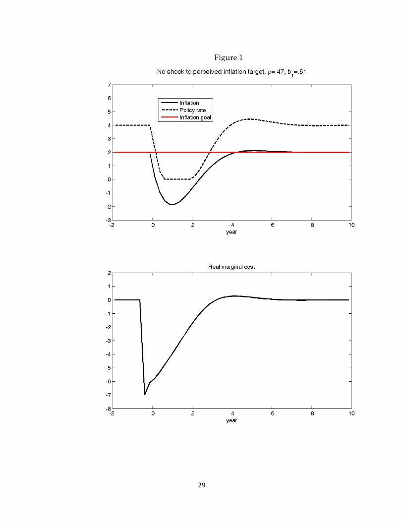
In the simulation of the model that follows, we start the economy at a quarterly level of real
marginal cost that is well below its equilibrium, reflective of recent readings for this series (see
footnote 3 above). The output gap begins at -2 percent, which is qualitatively consistent with
such low readings for marginal cost, but is still a modest gap given most current estimates. The
inflation rate begins at 2 percent, above its current value, and the true inflation target is 2
percent. The federal funds rate is at its long-run equilibrium, the sum of the long-run real
interest rate and the inflation goal. Given these starting conditions, the model then determines
the evolution of inflation, the funds rate, marginal cost, and output.8 Of course, this is an
optimistic starting point relative to current conditions, as inflation today is lower than the
implicit goal of the Fed, and despite uncertainty about the size of the output gap, it is not likely
that it is currently as small as -2 percent.9 Lowering the initial values for inflation and the
output gap would, of course, lower the trajectory for inflation and support the points below
even more strongly.10
7 See Barnes, Gumbau-Brisa, Lie, and Olivei (2009) for empirical evidence bearing on this point. 8 Marginal cost is linked to output in a way consistent with the simple derivation described in footnote 3, but allowing for a gradual adjustment to movements in output: 1 1 1 2 2t t t tmc mc b y b yω − − −= + +
. We set the parameters in the relationship to their full-sample estimates, obtaining the parameters
1 20.96, 0.45, 0.33b bω = = = − . 9 The data suggest a relationship between real marginal cost and the output gap that is described in the preceding footnote. 10 The shocks to marginal cost and output at the beginning of the simulations do not persist into subsequent periods. The model’s own propagation mechanisms account for the dynamics displayed in the figures.
9
The simulations are revealing. In the baseline simulation (Figure 1), we assume a degree of
indexation that is consistent with a standard “hybrid” model of inflation that mixes both
forward-looking and backward-looking (indexation) influences.11 In the baseline, there is no
misperception about the Fed’s inflation goal. Despite initially very well anchored inflation
expectations, the pull of depressed marginal cost on inflation is significant. Inflation drops well
below zero, the federal funds rate is pinned at the zero lower bound for about two years, and
inflation only gradually regains levels consistent with the Fed’s target. Again, this simulation is
decidedly optimistic, in the sense that it assumes that most of the decline in output is matched
by a decline in potential, and the model reflects no financial disruption during the recession.
Both would serve to further depress output, inflation, and the policy rate. But the simulation
serves to illustrate an important qualitative point: Even if one places no faith in the gap, the
enormous decline in (the proxy for) marginal cost acts as a powerful pull on inflation even in
the presence of perfectly anchored expectations.12
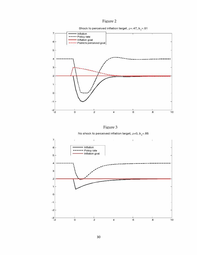
In the next simulation (Figure 2), the public initially believes that the Fed’s inflation target has
risen to 3 percent, shown in the dashed red line in the figure. Over time, the public will adjust
its perception of the target downward in line with observed inflation. But at first, this
misperception keeps inflation from falling as much as it does in the baseline simulation, as
price-setters expect a higher rate of trend inflation. As a consequence, the funds rate does not
have to fall as far, but it is still the case that on net, inflation falls well below zero for an
extended period, and the funds rate remains well below its equilibrium for several years. Thus,
in the model with significant indexation, these unanchored expectations, while important, do
not nearly offset the downward pressure on inflation that arises from depressed marginal costs.
The next figure (Figure 3) considers a simulation in which there is no indexation in the
economy, and thus no backward-looking inertia imparted to the inflation rate from this source.
11 The coefficients ρ and 1b in equation (1.5) are estimated using conventional techniques over the post-1984 sample. 12 While there are some differences in the paths of marginal cost across the four simulations, they are qualitatively similar, so we display the marginal cost path only for the first baseline simulation.
10
In this case, the overall disruption from the sharp drop in marginal cost is less severe: Inflation
declines, to be sure, dropping below one percent for a while, but after about three years it has
risen close to the target. The required decline in the federal funds rate is noticeably less.
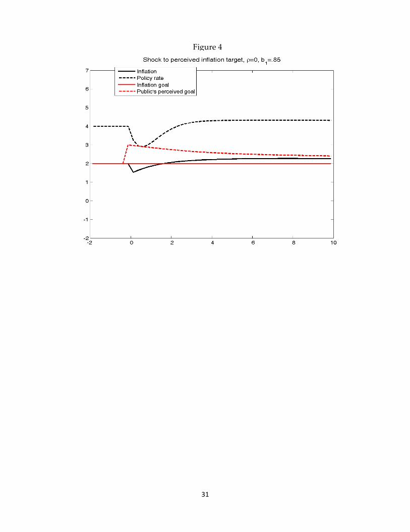
Under the same model assumptions, but allowing for the same misperception about the
inflation goal as in Figure 2, the inflation rate still declines, but is below target by less than a
percentage point and only for a fairly short time (Figure 4). The federal funds rate dips below its
long-run equilibrium for a bit, but because of the very forward-looking, flexible nature of the
economy in this model, the increase in the perceived inflation goal offsets most of the
downward pressure on inflation from marginal cost.
From these simulations, we offer the following conclusions:
• No matter the degree of indexation in the model, even with perfectly anchored
expectations, inflation is likely to fall in a recession characterized by the decline in
marginal cost (or the output gap) that we have seen to date.
• How much it falls, and how much monetary accommodation is required (and for how
long) is critically dependent on the degree of indexation or “backward-lookingness” that
characterizes inflation. In a very-forward-looking model, the decline in inflation may
well be modest.
• To date, the evidence on the persistence of inflation that bears on the degree of
indexation in this model is still mixed. Fuhrer (2009) examines a wide array of evidence
for recent samples and concludes that it would be risky to assume no persistence in
inflation for the United States, even in recent years. While persistence is likely to have
declined relative to the 1970s and 1980s, it probably remains a feature of inflation in the
United States. Thus, one should probably give some weight to a model with some
indexation. In these circumstances, well-anchored expectations do not prevent serious
downward pressure on inflation. Correspondingly, expectations that become un-
anchored on the upside do not offset much of the downward pressure on inflation.
11
Because the way expectations are formed and the degree of backward-lookingness in the
model matter importantly for how much expectations can offset the effects of marginal cost
or output, the next section examines empirically the influence of various expectations
concepts, including rational expectations, over the past 30 years.
III. What kind of expectations influence inflation? An empirical assessment
The expectations in the models described above are not observed in the same way as the federal
funds rate, inflation, and output are. In the economics literature of recent decades, this
unobservability has been circumvented by assuming “rational expectations”; the expectations of
interest are, in essence, the forecasts of the model in which they are embedded.13
But if the model fails to capture important aspects of the economic environment, then the
rational or model-consistent expectations may not represent well the expectations of real-world
economic actors. Alternatively, economists may wish to examine more direct measures of
inflation expectations to see how robust the conclusions from rational expectations models are
to different assumptions about expectations. Finally, much recent commentary has focused on
the stability (or lack thereof) in more direct measures of inflation expectations, positing that
well-anchored expectations may preclude a drop in inflation such as those that have followed
other significant postwar recessions. For any of these reasons, one may turn to proxies for
expectations, such as the forecasts of professionals, surveys of households or businesses, or the
expectations embedded in financial market prices.14
In this section, we use survey-based measures of inflation expectations to obtain another
measure of the importance of expectations in determining inflation. We run a “horse race” in a
13 This poses some methodological complications, as the equations include the expectations themselves. We leave this problem aside for the purposes of this brief. 14 Roberts (1997) provides one of the earliest examination of these inflation models with survey expectations.
12
simple inflation equation, allowing four different proxies for inflation expectations to determine
inflation. In addition to output or marginal cost, inflation is allowed to depend on:
1. Lagged inflation—here we employ the four-quarter moving average of inflation,
denoted 1avgtπ − in equation (1.6) below;
2. The rational (model-consistent) expectation of inflation;
3. The four-quarter-ahead forecast of inflation from the Survey of Professional
Forecasters (SPF), denoted 1Stπ in equation (1.6) below;
4. The 10-year forecast of inflation from the SPF, denoted 10Stπ in equation (1.6)
below.15
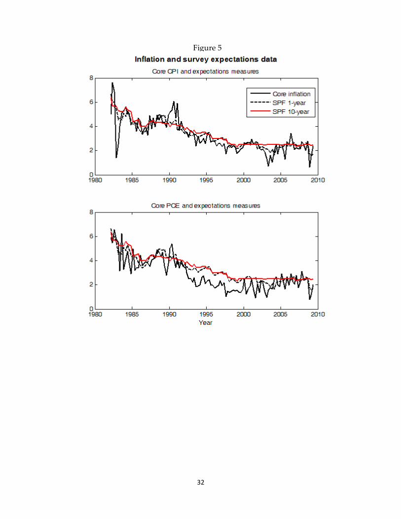
Figure 5 displays the data for the two SPF forecasts, along with the core CPI and PCE inflation
measures. Note that the 10-year SPF forecast has hovered very close to 2.5 percent since the late
1990s. This remarkable stability in the 10-year forecast is somewhat suspect to us. Recall that
this is the median forecast for the average inflation rate over the ensuing 10 years. As with a 10-
year bond, its longer maturity implies that it will be less responsive to near-term conditions
than a one-year forecast. But it would be unusual for a 10-year forecast (or a 10-year bond) to
remain within 10 basis points of a single value for over a decade. If the Fed had persuaded the
public that its inflation goal were 2.5 percent, then the one-year inflation expectation 10 years
hence could well remain fixed at 2.5 percent. But the rationale for a fixed median of 10-year
average forecasts is much harder to come by. The one-year SPF forecast, which, like the 10-year,
is plotted as of its forecast date, fluctuates considerably and tracks current inflation reasonably
well.
15 The University of Michigan one-year-ahead inflation expectation displays very similar properties to the SPF. In initial estimation testing, the differences between the Michigan and SPF forecasts were not qualitatively significant. The SPF 10-year expectation is the only consistently collected measure of longer-term inflation forecasts that is readily available. With more time, researchers will likely use the inflation expectations implied by the yields on TIPS, but at present, only a 10-year sample is available.
13
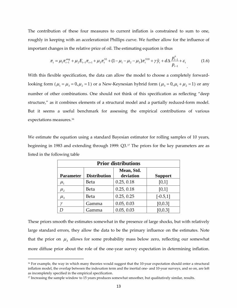
The contribution of these four measures to current inflation is constrained to sum to one,
roughly in keeping with an accelerationist Phillips curve. We further allow for the influence of
important changes in the relative price of oil. The estimating equation is thus
1 10 11 1 2 1 1 3 1 2 3
1
(1 )o
avg S S tt t t t t t t t
t
pE y dp
π µ π µ π µ π µ µ µ π γ ε−− − +
−
= + + + − − − + + ∆ +
. (1.6)
With this flexible specification, the data can allow the model to choose a completely forward-
looking form ( 1 3 20, 1µ µ µ= = = ) or a New-Keynesian hybrid form ( 3 1 20, 1µ µ µ= + = ) or any
number of other combinations. One should not think of this specification as reflecting “deep
structure,” as it combines elements of a structural model and a partially reduced-form model.
But it seems a useful benchmark for assessing the empirical contributions of various
expectations measures.16
We estimate the equation using a standard Bayesian estimator for rolling samples of 10 years,
beginning in 1983 and extending through 1999: Q3.17
These priors smooth the estimates somewhat in the presence of large shocks, but with relatively
large standard errors, they allow the data to be the primary influence on the estimates. Note
that the prior on 3µ allows for some probability mass below zero, reflecting our somewhat
more diffuse prior about the role of the one-year survey expectation in determining inflation.
16 For example, the way in which many theories would suggest that the 10-year expectation should enter a structural inflation model, the overlap between the indexation term and the inertial one- and 10-year surveys, and so on, are left as incompletely specified in the empirical specification. 17 Increasing the sample window to 15 years produces somewhat smoother, but qualitatively similar, results.
14
For example, the one-year survey could serve as a correction to the model-consistent
expectation, which might entail a non-positive coefficient. Similarly, the implicit prior on the 10-
year survey expectation spans a considerably larger region (from -2 to 1.5), reflecting the less
theoretically grounded role for this long-term expectation in the canonical inflation equation.
The priors on the indexation and rational expectation terms are a bit tighter, as theory suggests
they should fall between zero and one.
With the presence of rational expectations for inflation in period t+1, the model implicitly
requires expectations of the output gap (and/or marginal cost), as well as expectations for the
one-year and 10-year SPF expectations. For output and the federal funds rate, we include
unconstrained (VAR) equations in output, the funds rate, and inflation. The intercepts for these
equations are allowed to change for each sample period. We link marginal cost to output as in
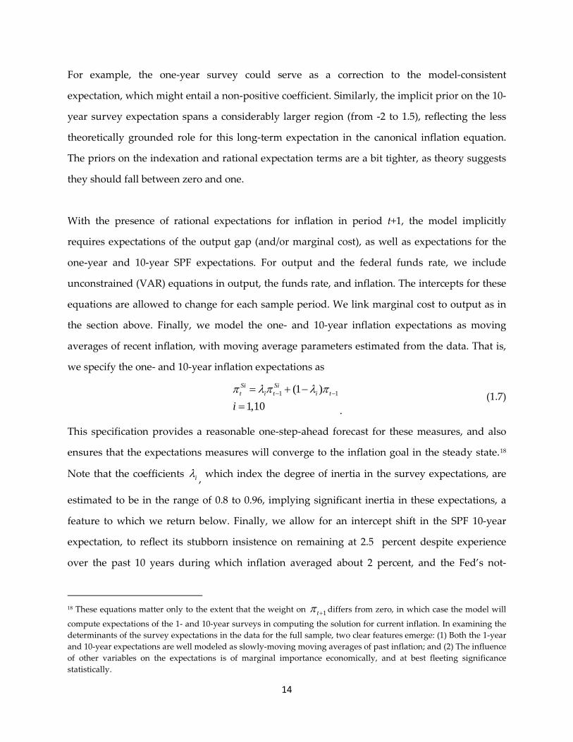
the section above. Finally, we model the one- and 10-year inflation expectations as moving
averages of recent inflation, with moving average parameters estimated from the data. That is,
we specify the one- and 10-year inflation expectations as
1 1(1 )1,10
Si Sit i t i t
iπ λπ λ π− −= + −= .
(1.7)
This specification provides a reasonable one-step-ahead forecast for these measures, and also
ensures that the expectations measures will converge to the inflation goal in the steady state.18
iλ
Note that the coefficients , which index the degree of inertia in the survey expectations, are
estimated to be in the range of 0.8 to 0.96, implying significant inertia in these expectations, a
feature to which we return below. Finally, we allow for an intercept shift in the SPF 10-year
expectation, to reflect its stubborn insistence on remaining at 2.5 percent despite experience
over the past 10 years during which inflation averaged about 2 percent, and the Fed’s not-
18 These equations matter only to the extent that the weight on 1tπ + differs from zero, in which case the model will
compute expectations of the 1- and 10-year surveys in computing the solution for current inflation. In examining the determinants of the survey expectations in the data for the full sample, two clear features emerge: (1) Both the 1-year and 10-year expectations are well modeled as slowly-moving moving averages of past inflation; and (2) The influence of other variables on the expectations is of marginal importance economically, and at best fleeting significance statistically.
15
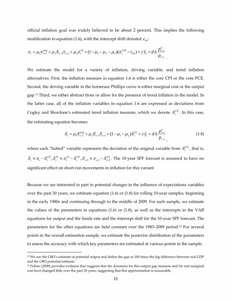
official inflation goal was widely believed to be about 2 percent. This implies the following
modification to equation (1.6), with the intercept shift denoted 10c :
1 10 11 1 2 1 1 3 1 2 3 10
1
(1 )( )o
avg S S tt t t t t t t
t
pE c y dp
π µ π µ π µ π µ µ µ π γ −− − +
−
= + + + − − − − + + ∆
.
We estimate the model for a variety of inflation, driving variable, and trend inflation
alternatives. First, the inflation measure in equation 1.6 is either the core CPI or the core PCE.
Second, the driving variable in the horserace Phillips curve is either marginal cost or the output
gap.19
CStπ
Third, we either abstract from or allow for the presence of trend inflation in the model. In
the latter case, all of the inflation variables in equation 1.6 are expressed as deviations from
Cogley and Sbordone’s estimated trend inflation measure, which we denote . In this case,
the estimating equation becomes
1 11 1 2 1 1 1 2
1
ˆ ˆ ˆ ˆ(1 )o
avg S tt t t t t t
t
pE y dp
π µ π µ π µ µ π γ −− − +
−
= + + − − + + ∆
, (1.8)
where each “hatted” variable represents the deviation of the original variable from CStπ , that is,
1 11 1 1ˆ ˆ ˆ, ,CS S S CS CS
t t t t t t t t tπ π π π π π π π π+ + +≡ − ≡ − ≡ − . The 10-year SPF forecast is assumed to have no
significant effect on short-run movements in inflation for this variant.
Because we are interested in part in potential changes in the influence of expectations variables
over the past 30 years, we estimate equation (1.6) or (1.8) for rolling 10-year samples, beginning
in the early 1980s and continuing through to the middle of 2009. For each sample, we estimate
the values of the parameters in equations (1.6) or (1.8), as well as the intercepts in the VAR
equations for output and the funds rate and the intercept shift for the 10-year SPF forecast. The
parameters for the other equations are held constant over the 1983–2009 period.20
19 We use the CBO’s estimate of potential output and define the gap as 100 times the log difference between real GDP and the CBO potential estimate.
For several
points in the overall estimation sample, we estimate the posterior distribution of the parameters
to assess the accuracy with which key parameters are estimated at various points in the sample.
20 Fuhrer (2009) provides evidence that suggests that the dynamics for this output gap measure and for real marginal cost have changed little over the past 30 years, suggesting that this approximation is reasonable.
16
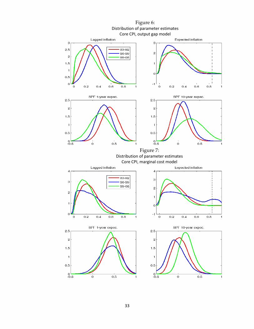
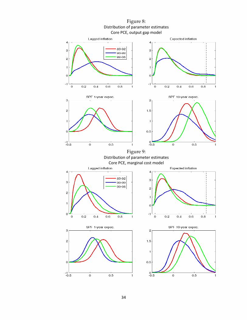
Figures 6–9 display the posterior distributions over the past three decades for the parameters iµ
that premultiply the expectations proxies.21 22 As the figures make clear, there is considerable
uncertainty about the precise contributions to core inflation measures from lagged inflation, the
model-consistent expectation of inflation, and the short- and long-term survey expectations
proxies.23
1. The weight on lagged inflation, often associated with so-called “intrinsic
persistence” of inflation, has been moderate over the past 30 years. For most
measures, its weight appears to have declined in the most recent decade.
This likely reflects collinearity among the survey measures and lagged inflation, as
well as the relatively low variability in inflation and marginal cost prior to the most recent
recession. Nonetheless, the results suggest some broad patterns across measures and time
periods.
2. Note that in principle, the model could replicate a purely forward-looking rational
expectations model by assigning weights of zero to lagged inflation and the survey
expectations measures. However, the weight on the rational expectation of next
quarter’s inflation is estimated to be small and insignificantly different from zero
throughout the decades across all inflation and driving variable measures. The
vertical line in the top-right panel of each figure indicates the value that this
parameter takes in the purely forward-looking simulation of the first section. In all
cases, the estimate places a tiny probability on this value.
3. In the most recent decade, the weight on the 10-year SPF expectation has risen for
some, but not all, measures. The most noticeable increase arises for the core CPI with
the output gap as the driving variable, Figure 6. In prior decades, it would have been
difficult to reject the hypothesis that the contribution from the 10-year expectation
21 These distributions are derived from estimates for rolling 10-year samples from 1983 to 2009, using the methods described in footnote 22. 22 The posterior is estimated using the now-conventional Markov-chain Monte Carlo method, with a Random-walk Metropolis-Hastings step. 23 In some cases, the posterior distribution differs little from the prior, suggesting that the likelihood (the data) offers little information about the parameter. In the text, we highlight those cases in which this is not true.
17
was zero. The core PCE model with real marginal cost as the driving variable shows
a more modest increase in the weight on the 10-year SPF forecast in the most recent
decade.
4. The weight on lagged inflation was particularly high for the core PCE/output gap
model in the 1990s.
5. For the CPI models, the one-year SPF forecast has a significant influence on inflation
for all of the subsamples. The influence of the one-year forecast is much less evident
for the PCE models.
While the shift towards some weight on the long-term expectation for some periods is of
interest, it is also important to note that the weight rises at precisely the time when the 10-year
forecast “flat-lines” at 2.5 percent. This could be taken as evidence that price-setters have well-
anchored expectations, but, as discussed above, one would not expect that well-anchored
expectations would manifest themselves as a constant forecast for the 10-year average inflation
rate.
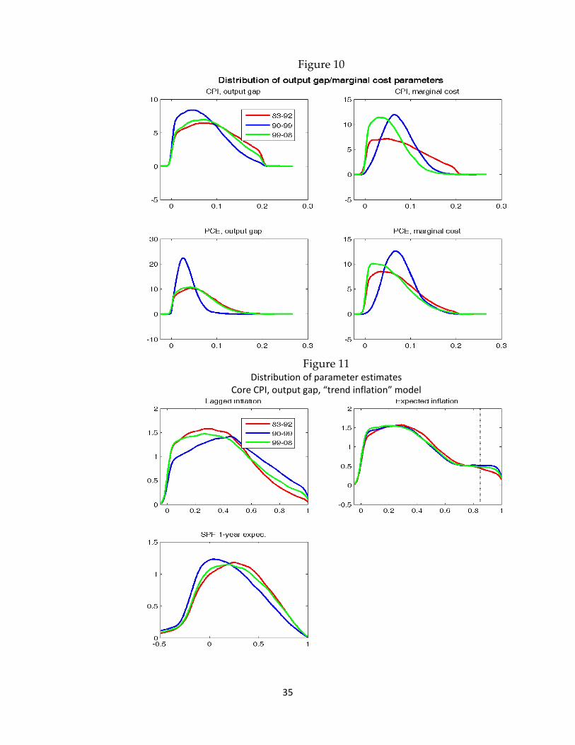
A key part of the debate over the determination of inflation is the role played by the output gap
or marginal cost. Figure 10 provides some evidence bearing on this question. It displays the
distribution of the estimated parameter on the output gap or marginal cost (γ ) for the four
models discussed above. In general, the estimated parameter is small, ranging from 0.02 to 0.06
across the decades, but in most cases, its accuracy has improved in the past decade. The data
generally reject the null that the parameter is zero. Typically only about 5 percent of the
estimated parameter’s distribution lies to the left of 0.01.
18
For the periods when the 10-year expectation is given near-zero weight, so that
1 2 31 0µ µ µ− − − = , one can rewrite the model of equation (1.6) so that it is approximately an
“inflation gap” model in which trend inflation is proxied by the 10-year expectation:24
10 10 10 1 10 11 1 2 1 1 3
1
( ) ( ) ( )o
S avg S S S S tt t t t t t t t t t
t
pE y dp
π π µ π π µ π π µ π π γ −− − +
−
− = − + − + − + + ∆
. (1.9)
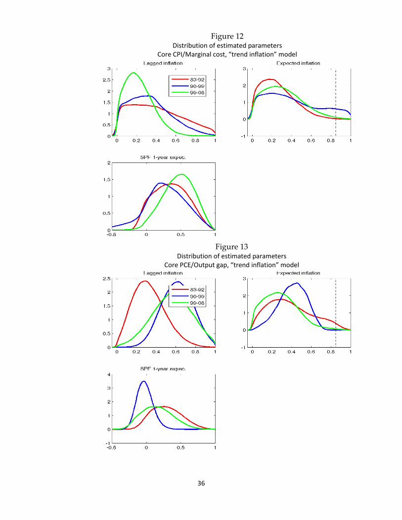
Because the results overall suggest that this inflation gap representation may be a reasonable
approximation, the next set of figures displays parallel results for an inflation gap model, in
which all of the inflation measures are expressed as deviations from Cogley and Sbordone’s
trend inflation estimate, and thus the estimating equation becomes equation 1.8. The results in
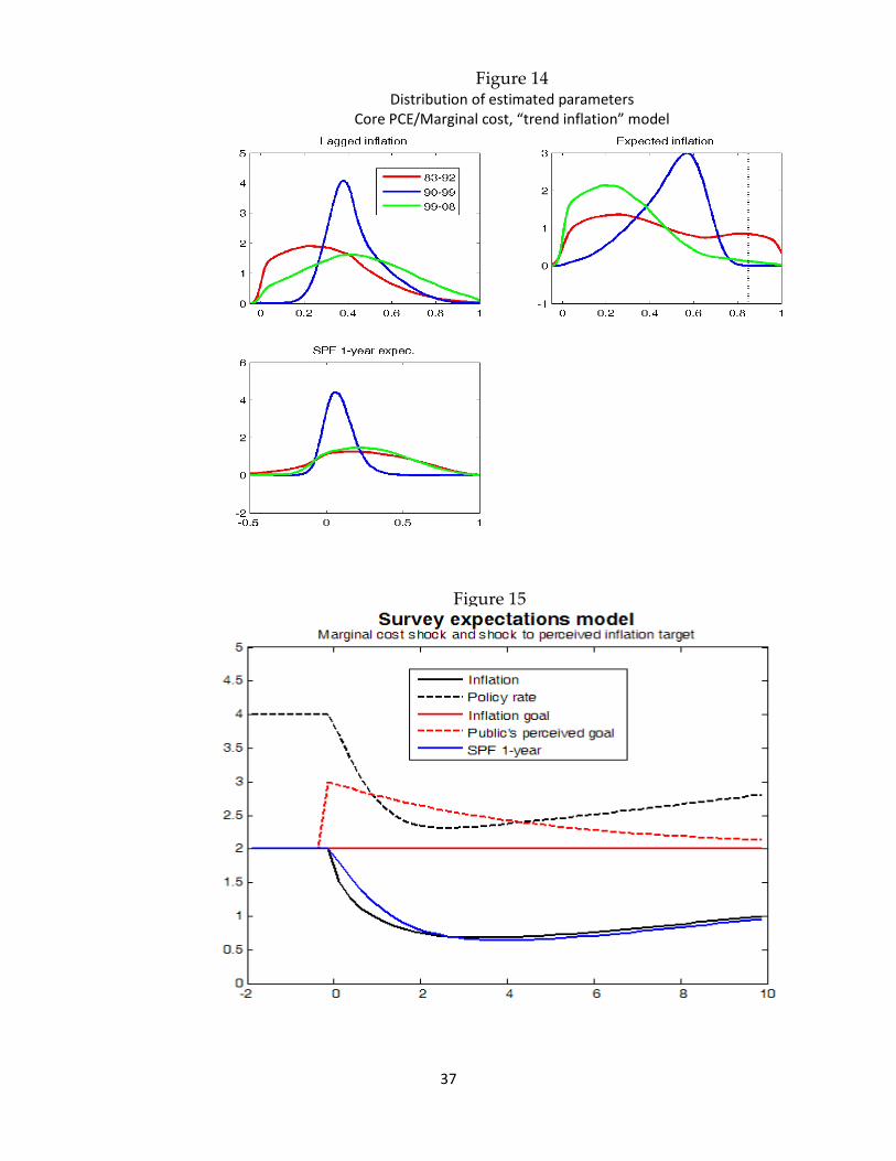
these cases, Figures 11–14, suggest a somewhat greater role for the one-year survey expectation
in the core CPI model, and a somewhat greater role for lagged inflation in the core PCE models.
The role of the rational expectations term is relatively limited. While it is not precisely
estimated, in the most recent decade (the green lines), its weight is typically low and usually not
significantly different from zero.
IV. The balance of expectations and marginal cost pressures in a survey-expectations-based model
The results in the preceding section suggest that inflation is not well characterized by a purely
forward-looking model, and these results appear to favor putting some weight on the survey
expectations (as well as on lagged inflation). Thus, it is of interest to revisit the simulation of a
model that uses survey expectations as the key expectation variable in an otherwise standard
dynamic stochastic general equilibrium model. We conduct a simulation like the one discussed
in Section II, but instead of rational expectations, we now use a model that is consistent with the
estimated influence of survey expectations from the preceding section.
24 The model would be exactly an inflation gap model if the timing of the 10-year expectation terms corresponded to the inflation measures from which it is subtracted. Because the 10-year expectation is highly persistent, this difference is of little practical consequence. Clark and Davig (2008) find that the underlying trend inflation component appears to be closely correlated to the 10-year SPF survey measure.
19
In particular, we assume that the influence of the longer-term inflation expectation primarily
reflects the influence of trend inflation, and we model trend inflation as in Section II (it
represents the very slow-moving inflation target of the Fed). We allow the one-year survey
expectation to influence current inflation in lieu of the model-consistent expectation. Thus, the
inflation equation becomes
11 1 1 3( ) ( )pub pub S pub
t t t t t t tmcπ π µ π π µ π π γ− −− = − + − + . (1.10)
To mimic the qualitative properties of the estimation results in the preceding section, we set
1 0.4µ = and 3 0.6µ = --inflation depends somewhat on lagged inflation, but more importantly,
it is strongly tied to the one-year (SPF) expectation of inflation. The equation for the one-year
SPF expectation is also expressed in deviations form
1 11 1 1 1( ) (1 )( )S pub S pub pub
t t t t t tπ π ω π π ω π π− − − −− = − + − − ,
which simply makes the deviation of the one-year expectation from the inflation trend a moving
average of past deviations of actual inflation from the inflation trend. As suggested in Figure 5
and discussed in footnote 18, the one-year SPF forecast is well modeled as a slowly moving
average of current and recent inflation realizations. Thus, for this exercise, we set ω to two-
thirds, which implies a slightly more rapid response to recent inflation than what we find in the
data.25
Figure 15 shows the response to the same large marginal cost shock for this survey expectations
model, with a shock to the public’s perceptions of the Fed’s inflation goal.26
25 The estimates of the process for the one-year forecast are performed on the raw, rather than detrended data. However, the trend inflation rate is presumed to move quite slowly, so that its contribution to the short-run movements of the one-year forecast will generally be small.
The significant
downward pressure exerted by below-equilibrium marginal cost is partly offset by the rather
slow downward progress of the one-year inflation expectation. This anchoring limits the decline
in inflation to a minimum of 0.7 in the second year of the simulation. But this same anchoring
26 The simulation without the misperception of the inflation goal (not shown) leads to quite similar results. With the strong weight on the one-year inflation expectation, the effect of the temporary shift in the inflation goal is fairly muted.
20
also slows the progress of inflation upward towards its (unchanged) goal of 2 percent. While
inflation has risen to 1 percent by the end of the simulation, it takes several more years to reach
its goal. To be sure, monetary policy could act more aggressively with the funds rate in this
simulation (if not in the real world). But the qualitative point of the simulation is clear: to the
extent that inflation of late has become more closely associated with slow-moving expectations
like those reflected in the SPF measures, this may limit the downward trajectory of inflation
somewhat. But it will also likely slow upward progress towards its long-run goal.27
V. Activity gaps and inflation dynamics
The inflation models and the related simulations considered in the previous section hinge on
activity gaps (or real marginal costs) being the driving process for inflation. Absent such a link
from activity to inflation, these models have no content. There is now a large literature on the
performance of inflation forecasts based on activity gaps (that is, Phillips curve representations
of inflation dynamics) relative to univariate benchmarks. Recent work by Stock and Watson
(2009) surveys the literature and provides a comprehensive analysis of Phillips curve forecasts
of inflation vis-à-vis good univariate benchmark models. The conclusion reached by Stock and
Watson after examining a wide array of (backward-looking) Phillips curve specifications is that
the link from activity gaps to inflation is not always present. Inflation is difficult to forecast, and
Phillips curve-based forecasts of inflation outperform univariate benchmarks only sporadically.
Stock and Watson, however, note that the episodes when activity-based forecasts outperform
univariate forecasts have in common a large activity gap, either positive or negative.
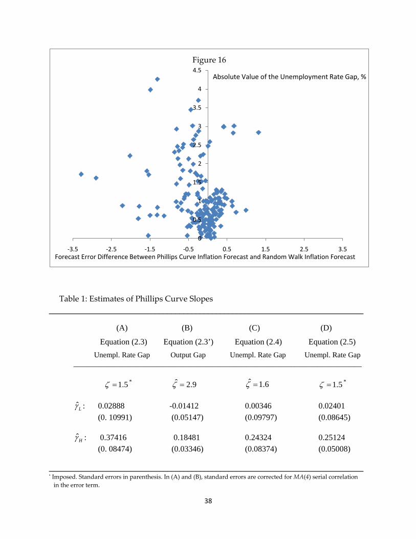
The point that large activity gaps may contain information for inflation forecasting is illustrated
in Figure 16. The figure compares inflation forecast errors based on a standard backward-
27 This feature would be qualitatively similar, although quantitatively exaggerated, with a 10-year expectation that mimicked the behavior of the SPF 10-year forecast. That variable is even more inertial, and would thus more forcefully limit the downward motion of inflation and would similarly slow even more strongly inflation’s progress towards its goal.
21
looking Phillips curve with the forecast errors based on a random walk model of inflation.
Specifically, the Phillips curve model takes the form
4 44 4( )t t t t ta L u zπ π γ χ υ+ += − + + , (2.1)
where 44tπ + denotes the four-quarter-ahead rate of inflation, tπ is the one-quarter (annualized)
rate of inflation, tu is the unemployment rate gap, tz is a vector of supply shocks, and 44tυ + is an
error term. As usual, the sum of the coefficients on the lags of inflation is constrained to sum to
unity. In the random walk model of inflation, the four-quarter-ahead rate of inflation is equal to
the rate of inflation over the most recent four quarters plus an error term:
4 4 44t t tπ π υ+ = + . (2.2)
The figure shows on the horizontal axis the difference between the absolute value of the forecast
error for four-quarter-ahead core PCE inflation based on the Phillips curve, and the absolute
value of the forecast error of four-quarter-ahead core PCE inflation when the inflation forecast is
given by the most recent historical value of four-quarter core PCE inflation. A negative value on
the horizontal axis implies that the Phillips curve-based forecast is more accurate than the
random walk univariate forecast, and vice versa. The variable on the vertical axis is the absolute
value of the unemployment rate gap, that is, the absolute value of the difference between the
unemployment rate and an estimated measure of the NAIRU. Each dot in the figure represents
a different quarter, and the period we consider is 1961: Q1 to the present. It is apparent from the
figure that when the unemployment rate gap is small, there is little to suggest that the Phillips
curve inflation forecasts are better than the random walk forecasts, as there are roughly as many
points to the left as there are to the right of the vertical axis. It is only when the gap starts to
become large in absolute value that there is a tendency for the points to be located to the left of
the vertical axis, implying that Phillips curve-based forecasts are more accurate than random
walk forecasts.
The Phillips curve based-forecasts embedded in Figure 16 are in-sample. Stock and Watson,
instead, work with out-of-sample forecasts. Moreover, they consider a variety of activity gap-
based specifications for modeling inflation, a different estimate for the time-varying NAIRU
22
than the one we are using, and a more sophisticated univariate forecast—though not materially
different in terms of forecast outcomes—than the simple random walk upon which this exercise
is based. Still, their evidence is broadly similar to the one depicted in the figure. Indeed, Stock
and Watson sum up their results as indicating that when the unemployment rate gap exceeds
1.5 percentage points in absolute value, the Phillips curve forecasts “improve substantially” (p.
146) upon the univariate model.
These findings are consistent with potential nonlinearities in the Phillips curve. Consider the
following modification to a standard backward-looking Phillips curve
( ) ( )4 44 4( )t t L t t H t t t ta L u I u u I u zπ π γ ζ γ ζ χ υ+ += − ≤ − > + + . (2.3)
The modification to the standard linear setup in (2.1) allows the tradeoff between inflation and
unemployment to change as a function of the level of the unemployment rate gap. There are
several ways of introducing this nonlinearity. In equation (2.3), we simply assume that the slope
of the Phillips curve can change according to whether the absolute value of the unemployment
rate gap lies below or above a threshold ζ , where ( )I ⋅ is an indicator function that takes the
value of one if the statement in parenthesis is true, and zero if the statement is false.28
ζ
Suppose,
consistent with the findings in Stock and Watson, that the threshold takes the value of 1.5
percent. Then, Lγ in equation (1) denotes the slope of the Phillips curve when the
unemployment rate gap is, in absolute value, below 1.5 percent, and Hγ denotes the slope of the
Phillips curve when the absolute value of the unemployment rate gap is above 1.5 percent.
Results from estimating (2.3) over the period 1961 to the present for core PCE inflation at a
quarterly frequency are reported in column (A) of Table 1. The slope is statistically significant
and economically relevant when the absolute value of the unemployment rate gap is above the
threshold, and not significantly different from zero when the absolute value of the
unemployment rate gap is below the 1.5 percent threshold. A formal statistical test rejects the
null hypothesis of the linear model (2.1) in favor of the nonlinear model (2.3) with the 1.5
28 For a more general specification where the threshold is not constrained to be the same in absolute value for negative and positive values of the gap, see Barnes and Olivei (2003).
23
percent threshold at standard confidence levels. Furthermore, searching over the threshold that
provides the best fit to the nonlinear model in equation (2.1) yields an estimated value for the
threshold ζ of 1.50 percent.
The Phillips curve models we consider in this section are based on the unemployment rate gap,
because much of the discussion in Stock and Watson about the usefulness of activity gaps in
informing inflation forecasts focuses on the unemployment rate. Similar results, however, hold
when the activity measure is given by the output gap. Consider the following nonlinear Phillips
curve model:
( ) ( )4 44 4( )t t L t t H t t t ta L y I y y I y zπ π γ ζ γ ζ χ υ+ += + ≤ + > + + , (2.3’)
where the only difference from the model in (2.3) is that we have replaced the unemployment
rate gap with the output gap. Estimates of the inflation-activity tradeoff and the threshold ζ are
provided in column (B) of Table 1. The estimated threshold for the absolute value of the output
gap is 2.9 percent. This value is consistent, from an Okun’s law standpoint, with the estimated
threshold for the unemployment rate gap in (2.3). The tradeoff is estimated to be statistically
and economically significant when the absolute value of the output gap is above the threshold,
but not so when the output gap is below the threshold. The null hypothesis of a linear
specification is rejected in favor of the nonlinear specification at standard confidence levels. The
similarity of findings when using the output gap in place of the unemployment rate gap also
extends to the rest of the analysis in this section. For this reason, in what follows we mention
only results concerning the unemployment rate gap.
It is possible to modify the model in (2.3) and proxy inflation expectations with a weighted
average of past inflation and long-run inflation expectations. Estimation results are largely
unaffected. The unemployment rate gap threshold is estimated at 1.51. The result (not reported)
that the slope of the Phillips curve is statistically significant and economically relevant when the
absolute value of the unemployment rate gap is above the threshold but not when the absolute
value of the unemployment rate gap is below the threshold continues to hold. Here, we briefly
24
consider an alternative specification that treats inflation expectations as an unobserved
component. The relationship we estimate now takes the form
( ) ( )4 44 4
et t L t t H t t t tu I u u I u zπ π γ ζ γ ζ χ υ+ += − ≤ − > + + , (2.4)
where
1e et t tπ π ν−= + .
In this setup, inflation expectations etπ are unobserved and follow a random walk, with tν
denoting an independent and identically distributed shock. Results from this estimation
exercise are reported in column (C) of Table 1. The absolute value of the unemployment rate
gap threshold is now estimated at 1.6 percent. The estimates continue to be consistent with the
view that the gap matters for determining inflation once the unemployment rate is sufficiently
far from the NAIRU.
These in-sample findings, together with the out-of-sample forecasting results of Stock and
Watson, provide some evidence that knowledge of a large unemployment rate gap contains
useful information about inflation. The results can also be reconciled with the Atkeson and
Ohanian (2001) findings that, from 1984 on, the random walk characterization of inflation
provides better inflation forecasts than the forecasts obtained from a Phillips curve. Excluding
the current recession, there have been few episodes when the unemployment rate gap was
above or below the 1.5 percent threshold. To some extent, the enumeration of these episodes
depends on the way the NAIRU is estimated. Starting in 1984 and excluding the present period,
one can estimate with some confidence the unemployment rate to be sufficiently far away from
the NAIRU at the beginning of the sample and during the recession of the early 1990s, and with
much more uncertainty during a few quarters late in the 1990s’ expansion (when the
unemployment rate bottomed at 3.9 percent) and after the 2001 recession (when the
unemployment rate peaked at 6.1 percent in 2003). The proximity of the unemployment rate to
the NAIRU for most of the post-1983 period could then explain the Atkeson and Ohanian
results, and possibly also the fact that the in-sample estimates of the slope of the Phillips curve
25
(in standard linear settings) are not particularly significant statistically and/or relevant from an
economic standpoint.
While there is uncertainty about the extent of activity gaps in many circumstances, the most
recent reading of the unemployment rate at 9.9 percent in April 2010 should place the
unemployment rate gap well above the 1.5 threshold that seems to make knowledge of the gap
useful for forecasting inflation. More debatable is the extent of the downward pressure that
such a gap will exert on inflation. As the previous sections show, this will depend importantly
on how inflation expectations are formed. Too, it will depend on the size of the gap and the
slope of the Phillips curve. In this respect, it is interesting to assess the performance of a simple
threshold Phillips curve model of inflation in the current situation. Since the four-quarter-ahead
inflation model in (2.3) leaves limited scope for considering the dynamics of inflation in the
most recent quarters, we use a one-quarter-ahead inflation specification
( ) ( ) 11 1( ) 1.5 1.5t t L t t H t t t ta L u I u u I u zπ π γ γ χ υ+ += − ≤ − > + + , (2.5)
where we have imposed a 1.5 percent unemployment rate gap threshold. We estimate (2.5) on
core PCE inflation over the period 1961-to-2004. We then perform a dynamic simulation over
the subsequent period. In the simulation, we provide actual values for the unemployment rate
gap u and the supply shocks z , while only the projected values of inflation enter the
simulation. Column (D) of Table 1 reports the estimates for the parameters Lγ and Hγ in (2.5).
Again, the inflation-unemployment tradeoff is significant only when the unemployment rate
gap is larger than 1.5 percent in absolute value.
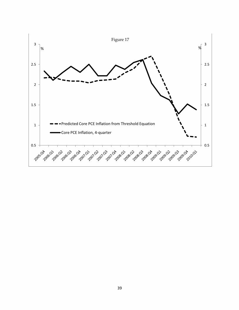
Results of the dynamic simulation are shown in Figure 17. The figure reports actual and
simulated values for four-quarter core PCE inflation starting in 2005: Q4.29
29 This is the first period in the simulation where only forecast values of inflation enter in (2.5).
Predicted inflation
tracks actual inflation reasonably well. Still, it is also apparent that over the most recent quarters
predicted inflation has been on a steeper downward trend than actual inflation. Given the
estimates in column (D) of Table 1, an average unemployment rate gap of about 4 percent over
26
the next four quarters implies a further drop in four-quarter core PCE inflation of roughly 1.2
percent, other things being equal. It is possible that the estimates reported in Table 1 when the
unemployment rate gap lies above the threshold could underestimate the current sacrifice ratio.
Some studies (see Tetlow and Ironside 2007) provide evidence of a flattening of the Phillips
curve in most recent years, with a consequent increase in the sacrifice ratio. As already
mentioned, this could be the result of weak identification stemming from the very few instances
of large unemployment rate gaps. But it could suggest also that inflation behavior at the very
low levels of inflation we have been experiencing in the most recent years is fundamentally
different from inflation behavior when the average level of inflation is comparable to the levels
experienced during the 1970s, 1980s, and early 1990s.
What do these results imply for the interpreting the recent behavior of inflation, and for the
current forecast?
VI. Conclusions
Given the difficulties in modeling inflation, especially over the past decade when inflation has
been relatively tranquil, and the economy—up until 2007—was similarly placid by historical
standards, we should be hesitant to draw any conclusions too firmly.
That said, the analysis presented in this paper points to some tentative conclusions about
inflation and its likely trajectory over the coming years:
1. With all of the models discussed in this paper, the current configuration of output gaps
(however poorly estimated) and marginal cost suggest that inflation is likely to remain
low, perhaps declining, and below the Federal Reserve’s implicit goal for several years.
2. Within more formal models of inflation, apart from the extreme position of a purely
forward-looking model, there are significant downside risks to inflation, even if
expectations are very well anchored.
27
3. Evidence on the influence of survey measures of inflation expectations on current
inflation suggests that model-consistent expectations have not reflected well the
expectations that have influenced CPI or PCE inflation over the past three decades. The
effect of lagged inflation has been large at times, but appears to have declined in recent
years.
4. Expectations that are well proxied by slow-moving survey expectations appear to have
had some influence over the decades, and, for some models, that influence has increased
recently.
5. In a model that substitutes slow-moving survey expectations measures for model-
consistent expectations, the forecast for the near term envisions a decline in inflation that
is somewhat more muted. In this sense, the risks to more pronounced disinflation could
be mitigated by well-anchored inflation expectations. Correspondingly, however, the
time required for inflation to rise to its FOMC-determined goal will be quite long.
6. While there are numerous issues surrounding the measurement and definition of the
output or unemployment gap that sits at the center of many inflation models, evidence
in this paper is consistent with that of Stock and Watson (2009). Both they and we find
that in periods characterized by what appear to be large output gaps (such as the current
period), gaps are important predictors of inflation.
7. Altogether, these observations suggest that, across a fairly wide array of inflation
frameworks, one would expect inflation to decline in the near term. Precisely how much
depends on key parameters of the model, about which we must admit a fair amount of
uncertainty. But one extreme among the alternative inflation models—a purely forward-
looking model with little effect from inertial variables, such as the one depicted in
Figures 3 and 4—appears to be significantly at odds with the data. It could be risky to
count too much on the implications of such a framework.
28
References Atkeson, A., and L. Ohanian (2001). “Are Phillips Curves Useful for Forecasting Inflation?” Federal Reserve Bank of Minneapolis Quarterly Review 25(1): 2–11 (Winter).
Barnes, M., and G. Olivei (2003). “Inside and Outside Bounds: Threshold Estimates of the Phillips Curve.” New England Economic Review: 3–18.
Barnes, M., F. Gumbau-Brisa, D. Lie, and G. Olivei (2009). “Closed-Form Estimates of the New Keynesian Phillips Curve with Time-Varying Trend Inflation.” Working Paper (November).
Clark, T., and T. Davig (2008). “An Empirical Assessment of the Relationships Among Inflation and Short- and Long-Term Expectations,” Working Paper (October). Cogley, T., and A. Sbordone (2008). “Trend Inflation, Indexation, and Inflation Persistence in the New Keynesian Philips Curve.” American Economic Review, 98(5): 2101–2126. Fuhrer, J. (2009). “Inflation Persistence,” chapter prepared for the new Handbook of Monetary Economics. Federal Reserve Bank of Boston Working Paper (November). Gordon, R. J. (1982). “Price Inertia and Policy Ineffectiveness in the United States, 1890–1980.” Journal of Political Economy 90(6): 1087–1117. Roberts, J. (1997). “Is Inflation Sticky?” Journal of Monetary Economics 39(2): 173–196. Rotemberg, J., and M. Woodford (1997). “An Optimization-Based Econometric Framework for the Evaluation of Monetary Policy.” NBER Macroeconomics Annual 1997, 12: 297–361. Stock, J. and M. Watson (2007). “Why Has Inflation Become Harder to Forecast?” Journal of Money, Credit and Banking 39 (s1): 3–33. Stock, J., and M. Watson (2009). “Phillips Curve Inflation Forecasts,” in Understanding Inflation and the Implications for Monetary Policy: A Phillips Curve Retrospective, proceedings of the Federal Reserve Bank of Boston’s 2008 annual economic conference, Cambridge, MA: MIT Press. Taylor, J. (1993). “Discretion Versus Policy Rules in Practice.” Carnegie-Rochester Conference Series on Public Policy 39: 195–214. Tetlow, R. and B. Ironside (2007). “Real-Time Model Uncertainty in the United States: The Fed, 1996–2003.” Journal of Money, Credit and Banking 39(7): 1533–1561.
Table 1: Estimates of Phillips Curve Slopes _____________________________________________________________________________
(A) (B) (C) (D)
Equation (2.3) Equation (2.3’) Equation (2.4) Equation (2.5) Unempl. Rate Gap Output Gap Unempl. Rate Gap Unempl. Rate Gap _____________________________________________________________________________
_____________________________________________________________________________ * Imposed. Standard errors in parenthesis. In (A) and (B), standard errors are corrected for MA(4) serial correlation in the error term.
0
0.5
1
1.5
2
2.5
3
3.5
4
4.5
-3.5 -2.5 -1.5 -0.5 0.5 1.5 2.5 3.5
Figure 16
Forecast Error Difference Between Phillips Curve Inflation Forecast and Random Walk Inflation Forecast
Absolute Value of the Unemployment Rate Gap, %
39
0.5
1
1.5
2
2.5
3
0.5
1
1.5
2
2.5
3Figure 17
Predicted Core PCE Inflation from Threshold Equation