The Role of Extension and Sustainable Soil Management in Smallholder Agriculture – Evidence from Ethiopia – Dissertation to attain the doctoral degree of the Faculty of Agricultural Sciences Georg-August-University Goettingen, Germany presented by Denise Hörner born on June 18, 1988 in Wertheim, Germany Göttingen, March 2020
Transcript
The Role of Extension and Sustainable Soil Management
in Smallholder Agriculture
– Evidence from Ethiopia –
Dissertation
to attain the doctoral degree
of the Faculty of Agricultural Sciences
Georg-August-University Goettingen, Germany
presented by
Denise Hörner
born on June 18, 1988 in Wertheim, Germany
Göttingen, March 2020
First supervisor: Prof. Dr. Meike Wollni
Second supervisor: Prof. Dr. Matin Qaim
Third supervisor: Prof. Dr. Bernhard Brümmer
Date of oral presentation: 12.05.2020
Date of dissertation: 28.05.2020
i
Summary
Rising demand for agricultural commodities coupled with population growth, climate change,
declining soil fertility, environmental degradation and rural poverty in the developing world
call for strategies to sustainably intensify agricultural production. Sustainable intensification
refers to increasing production from the same area of land while reducing its negative environ-
mental consequences. Most of the adverse conditions are particularly prevalent in Sub-Saharan
Africa (SSA), where rates of undernutrition are the highest worldwide, while agricultural
productivity is still far below global averages. An important factor in explaining productivity
deficits among smallholders in SSA is the slow adoption of new agricultural technologies. Re-
cently, governments and international donors especially concentrate on the promotion of ‘sys-
tem technologies’, i.e. packages of technologies that should be applied jointly due to synergistic
effects. Yet, evidence shows that farmers delay in particular the uptake of system technologies,
and tend to scatter practices across plots instead of combining them on the same plot. Hence,
analyzing how to effectively enhance the adoption of technology packages is crucial, but still
understudied. In addition, comprehensive studies on the plot- and household level effects of
system technologies that use micro data from farmer surveys are still scarce when it comes to
impacts beyond traditional outcomes, such as crop yields and income, but important to under-
stand the consequences of adoption for farmers.
This dissertation addresses these gaps by studying the adoption and effects of ‘Integrated
Soil Fertility Management’ (ISFM). ISFM is a system technology comprised of a set of site-
specific soil fertility practices which should be applied in combination. Its core is the integrated
use of organic and inorganic fertilizers with improved seeds. Practices should be adapted to
local conditions, accompanied by a general improvement of agronomic techniques and, depend-
ing on the context, by other technologies such as crop rotation, agroforestry or reduced tillage.
The general aim of ISFM is an improvement of the soil’s fertility by replenishing its nutrient
stocks and organic matter level. Enhanced soil fertility is likely to improve food security, in-
comes, and ultimately, livelihoods of the rural population depending on small-scale agriculture.
In addition, healthier and more fertile soils can contribute to restoring and conserving natural
resources by providing crucial ecosystem services, such as the storage of soil carbon, erosion
control and the prevention of further deforestation. Thus, they can make an important contribu-
tion to the sustainable intensification of smallholder agricultural systems. However, ISFM com-
monly also goes along with increased demand for capital and labor, which often prevents small-
holders from adopting it. In addition, ISFM is considered knowledge-intensive, as combining
ii
several practices and adapting them to local conditions requires at least a basic understanding
of biological processes.
Against this background, the dissertation addresses two broad research objectives: Firstly,
to assess the role of ‘farmer-to-farmer’ and non-traditional forms of agricultural extension to
enhance knowledge and adoption of ISFM as a pathway to sustainable intensification. And
secondly, to assess the productivity and welfare implications of adopting ISFM practices at the
plot and household level. The thesis comprises three essays. The first essay concentrates on
knowledge and adoption of ISFM as a complex agricultural technology, while the second and
third essay analyze the effects of ISFM at the plot, respectively household level. All three essays
build on primary data collected among 2,382 farm households in the three Ethiopian regions
Amhara, Oromia and Tigray. The research was carried out in cooperation with the ‘Integrated
Soil Fertility Management Project’ (ISFM+ project) of the German Agency for International
Cooperation (GIZ), launched in 2015 in 18 districts in the three highland regions.
The first essay focusses on the role of agricultural extension in the dissemination of ISFM. In
recent decades, decentralized and participatory extension models have become dominant in
SSA. In these ‘famer-to-farmer’ approaches, only a few ‘model farmers’ are trained directly by
extension agents and should then train other farmers, often organized in groups. From there,
information should trickle down to all other households in a community. Yet, evidence suggests
that information diffusion is a complex process and does not automatically reach all farmers.
On the contrary, knowledge is likely to be transmitted incompletely from model farmers to
extension group members and from there to ‘ordinary’ farmers. This applies in particular to
complex system technologies, where farmers have to learn about each individual practice as
well as the necessity of applying them jointly. In this article, we assess the effects of a farmer-
to-farmer extension model and an additional intervention in form of a video on farmers’
knowledge and adoption of ISFM. We implemented a cluster randomized controlled trial, using
161 microwatersheds (mws) as primary units of randomization. 72 mws received the farmer-
to-farmer extension treatment, with model farmers who maintain ISFM demonstration plots and
train so-called ‘farmer research and extension groups’ as core elements. 36 out of these treat-
ment mws received an additional video intervention, explaining the underlying reasons for
adopting the ISFM package, and featuring documentaries on successful ISFM adoption. 89 mws
did not receive any intervention and serve as control group. In each of the three groups, 15
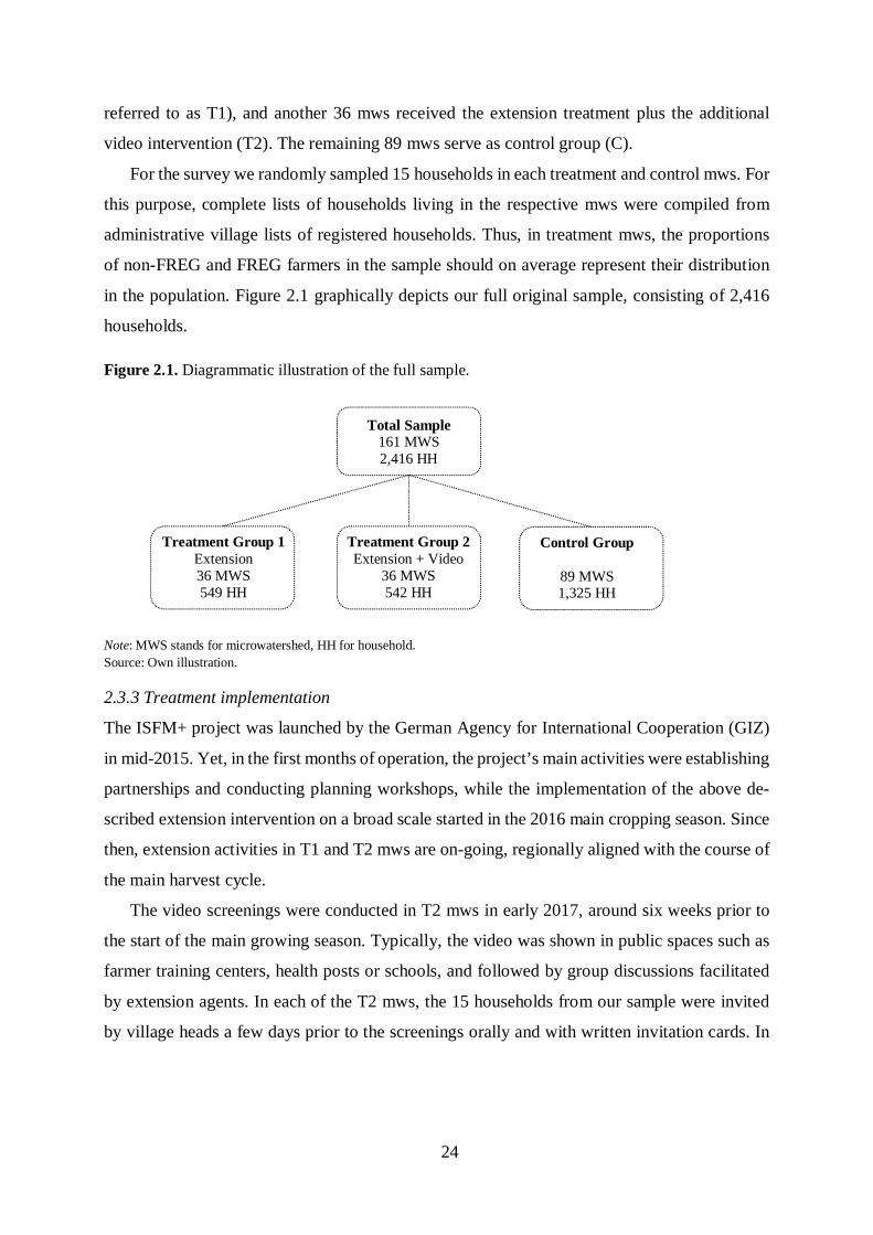
households per mws were randomly selected to be included in the sample. Findings show that
farmer-to-farmer extension, both alone and in combination with video, increases ISFM
iii
adoption, both of its individual components as well as their combined adoption on the same
plot. Effects are stronger for farmers who are involved in group-based extension activities, but
exist to a weaker extent also for farmers in the same communities who are not involved. On
average, we find no significant additional effect of the video intervention on adoption. How-
ever, the video does show a significant additional effect for farmers in treatment mws who are
not members of extension groups, in particular when it comes to the integrated use of the prac-
tices on the same plot. Further, while both farmer-to-farmer extension alone and in combination
with the video induce gains in ISFM knowledge, effects are significantly stronger for the com-
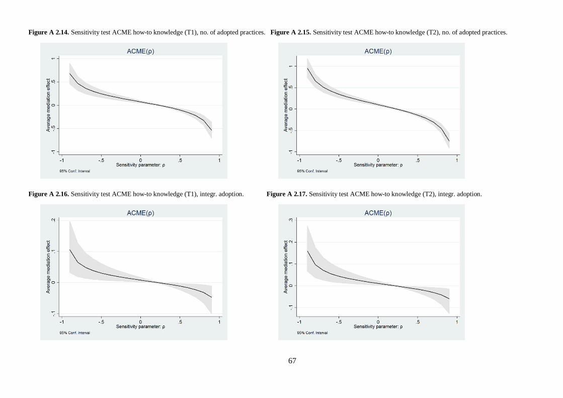
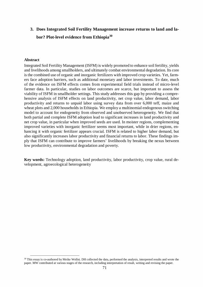
bined treatment. A causal mediation analysis reveals that increases in knowledge explain part
of the treatment effects on adoption. Overall, these results suggest that farmer-to-farmer exten-
sion can effectively foster technology adoption; both among extension group members as well
as among non-members residing in the same communities, probably a sign of information spill-
overs. Yet, for the non-members, providing complementary information via video seems a val-
uable method to counterbalance incomplete information diffusion and ultimately, foster the
adoption of complex system technologies such as ISFM.
Essay two analyzes of the effects of different combinations of ISFM practices on land produc-
tivity, net crop value, labor demand, labor productivity and financial returns to unpaid labor at
the plot level. To date, evidence on the profitability of ISFM in smallholder settings is scarce,
in particular when it comes to labor investments. The study differs from previous research by
looking into a broader range of outcome indicators, and into the effects of distinct combinations
of inorganic fertilizer, organic fertilizer and improved seeds. We employ a multinomial endog-
enous switching model to account for endogeneity, and data from over 6,000 teff, wheat and
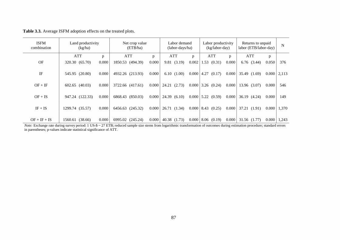
maize plots. Results show that both partial and complete ISFM adoption lead to significant
increases in land productivity and net crop value, in particular when improved seeds are used.
On average, the largest effect on land productivity stems from adopting complete ISFM, i.e.
improved varieties with inorganic fertilizer and organic fertilizer, followed by the combinations
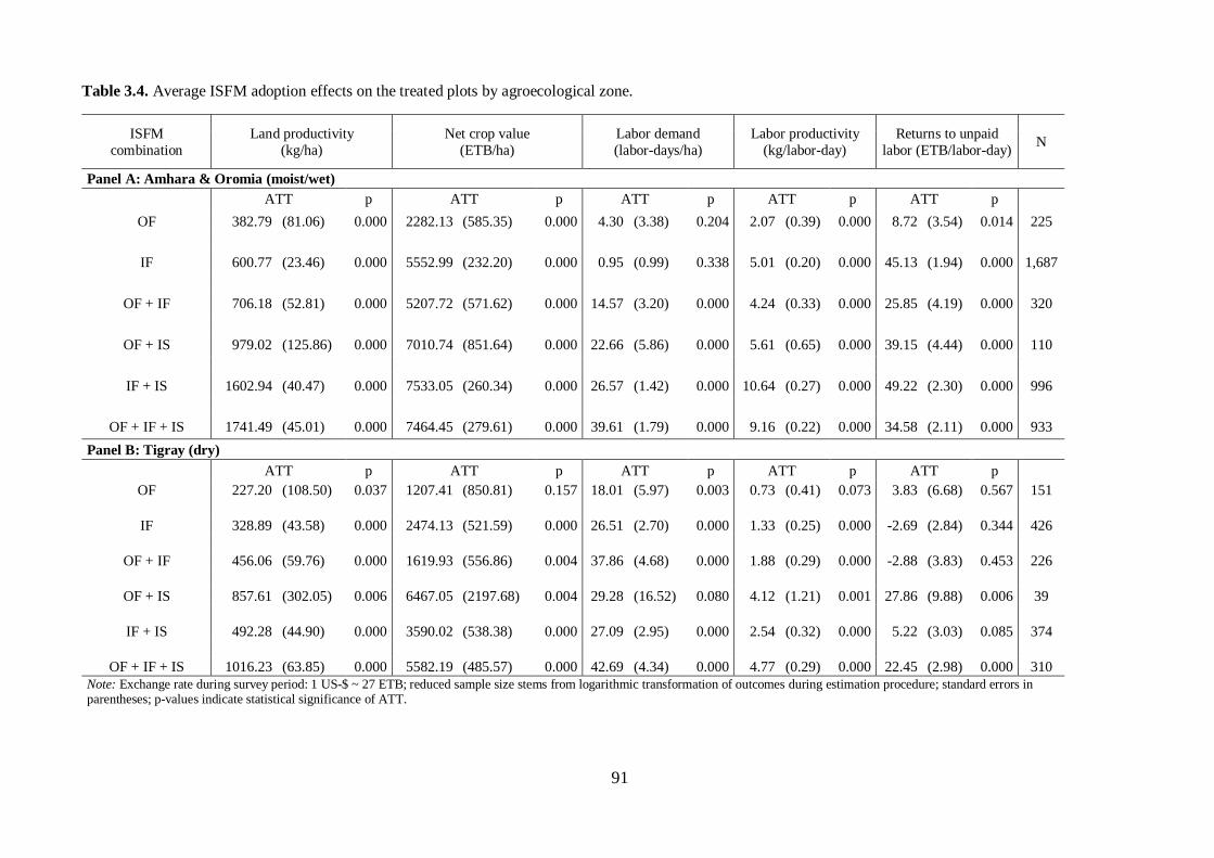
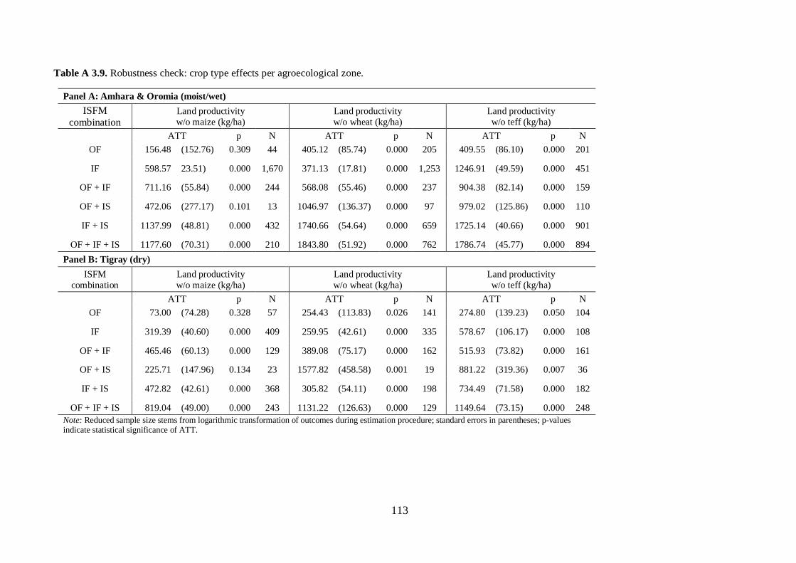
containing only one fertilizer type. Analyses for two different agroecological zones suggest that
in moister regions, complementing improved varieties with inorganic fertilizer is most im-
portant, while in drier regions, enhancing it with organic fertilizer is crucial, most probably due
to its water-retaining effect. Regarding net crop value, average effects of combining improved
seeds with either one or both fertilizer types are similar, despite the larger effect of the complete
package on land productivity; probably due to reduced input costs when only one of the two
fertilizer types is used. Further, as expected, ISFM is related to higher labor demand, but also
iv
significantly increases labor productivity and financial returns to labor. Hence, despite the ad-
ditional demand for labor and capital, results suggest that ISFM can be a profitable technology
for smallholders, at least when assessed at the plot level.
The third essay complements the picture on ISFM effects by analyzing its impacts at the house-
hold level. This is important since additional demand for resources associated with a technology
(package) may imply a reallocation of labor from one income-generating activity to another,
leaving net effects for a household uncertain. Therefore, we study whether adopting ISFM on
at least one teff, wheat or maize plot increases income obtained from these crops, as well as
total household income and household labor demand, and whether ISFM adoption is related to
the probability of pursuing other economic activities. In addition, we assess impacts on food
security, measured by self-reported incidences of food deprivation. Further, the essay analyzes
effects on children’s education as indicator for longer-term welfare, assessed by the enrollment
rate of children in primary school age, the average number of absent school days and average
educational expenditure. On the one hand, additional labor requirements may increase the work
burden for children, with possible negative effects for their education. On the other hand, if
ISFM is related to income gains, it might also lead to additional investments in education. We
apply the inverse probability weighting regression adjustment method to account for selection
bias, with propensity score matching as robustness check, and account for dissimilar agroeco-
logical potential by running disaggregated analyses for moist and dry regions. Results show
that ISFM adoption for main cereal crops is related to increased income per capita obtained
from these crops in both agroecological zones. Effects sizes of a rather lax definition of ISFM
– having used improved seeds in combination with at least either organic or inorganic fertilizer
– and a stricter definition, which comprises both fertilizer types, are very similar. A reason for
that might be the additional costs associated with using two instead of only one fertilizer type;
or because the synergistic potential of their joint use does not materialize immediately. Yet,
only in the moister regions, higher crop income seems to translate into higher household income
per capita, while it does not in the dry region. This might be because the share of income from
these crops in total household income is not important enough in the latter subsample. Yet, in
the dry region, ISFM adoption for main cereals also leads to a lower probability of achieving
income from other crops and off-farm activities, probably an effect of resource reallocation (in
particular labor). Moreover, we find a food security-enhancing effect of ISFM only for the
moister areas, but not for the dry region. In both subsamples, ISFM adoption is related to in-
creased demand for household labor. Yet, despite the higher labor demand, we find no
v
indication for increased school absenteeism or even reduced enrollment rates of children, and
no effects on educational expenditure. By contrast, ISFM adoption is associated with higher
primary school enrollment the moist agroecology. Hence, only for areas where ISFM adoption
is related to gains in overall household income, we also find positive effects on other welfare
indicators, such as food security and education. All in all, these results suggest that broader
welfare effects of agricultural innovations have to be evaluated within the complex system of
households’ income diversification strategies.
Overall, this dissertation contributes to the state of research by drawing a more comprehensive
picture of the effects of ISFM in resource-constrained and diversified smallholder systems, as
well as of interventions to foster the adoption of ISFM, or system technologies in general.
Firstly, results imply that farmer-to-farmer and other, not traditional forms of agricultural ex-
tension have the potential to increase knowledge and adoption of complex innovations. Yet,
extension systems still have to overcome shortcomings and find ways to be more inclusive,
probably by means of an effective and creative mix of interventions. And secondly, findings
suggest that ISFM can be a profitable technology for farmers, but also requires more resources.
When evaluating broader impacts of its adoption, it is important to account for heterogeneous
conditions and contexts.
vi
Acknowledgements
Writing this thesis would not have been possible without the support of many people. First of
all, I want to thank my first supervisor Prof. Dr. Meike Wollni for all the advice, guidance,
encouragement and trust in my ideas. You left me a lot of freedom to pursue my own path, but
made sure that I don’t lose track. I am particularly thankful for the support in drafting and
submitting our DFG grant application, which allowed me to carry out a randomized controlled
trial including a large-scale data collection. I enjoyed and learned a lot during our discussions,
and your support has certainly shaped my development as a researcher.
I would further like to thank my second and third supervisors, Prof. Dr. Matin Qaim and Prof.
Dr. Bernhard Brümmer. Your feedback from discussing my work during doctoral seminars,
brownbags and beyond was very valuable and encouraging, and contributed to refining my
research ideas and papers. I also thank Prof. Dr. Markus Frölich for including me in an on-
going project, being open to my ideas, and for helpful feedback at different stages.
I am grateful for the financial support of the DFG, through both the membership in the
RTG1666 GlobalFood and the grant number 390367541, that allowed me to carry out this re-
search project. In this regard, I want to gratefully mention the excellent management of the
RTG – in particular through Prof. Qaim and Dr. Melanie Grosse – and all the possibilities that
the RTG membership offered, regarding research, but also for the professional and personal
development beyond. I would also like to thank Jessica Torluccio, Gönül Yildirim and Ivanna
Beatriz Valverde Bajaña for your support with my project.
My special gratitude goes to all members of the GIZ-ISFM+ project team, in particular Steffen
Hibret Belay, Belay Taddese, Legesse Gelaw, Likissa Kurmana, and all other staff members. I
am incredibly thankful for your open-mindedness, positive team spirit and all the intellectual
and logistical support you provided me! I am happy we made this cooperation between aca-
demics and practice a success with mutual benefits. Keep up the good spirit and I wish you
many more achievements with the project!
Yemane Tsegaye and Yidnekachew Shumete from Epic Media Productions: thank you very
much for the fantastic work in producing the video intervention, your creative ideas and
vii
professionality made this a success. A special thanks to Yemane and Aka for your great friend-
ship and giving me a home in Addis!
I further want to thank the large team of enumerators and field assistants during all phases of
the project, in particular Ibrahim Worku for excellent co-coordination of the field work. Thank
you all for your motivation and dedication to the project, I really enjoyed working with you. A
special thanks goes to all the Ethiopian farmers who gave their time – nothing would have been
possible without your willingness to share your information and experiences!
Göttingen would not be Göttingen without all the great people. Thanks a lot, to all my col-
leagues and friends from the Chair, GlobalFood and beyond, for the inspiring environment,
constructive discussions and numerous cheering-up coffees and lunches. A special thanks to
Lisa, Kathrin, Andrea, Hanna, Katrin, Dirk, Luis, Jessie, Jorge, Fabi, Nadjia, Vivi – for runs up
the forest, unforgettable wine, beer or Salsa nights, great trips to cities, the mountains or the
seaside, and many more activities inside and outside of Göttingen. I am grateful you stay part
of my life as friends! Thanks to Zewdu, Peter, Lisa and Manuel for your helpful feedback
throughout and in the final phase of my PhD. Thanks to Paula, Armin and Gustav, especially
for your reliable culinary support during the last days. To Katrin: I can’t imagine a better person
to have started and now end this journey with – thanks a million for your bad jokes, support
and friendship!
On the same note, I cannot imagine my life without all my great friends from different phases.
Thank you for your invaluable support and the fun times together, which gave me the strength
to pursue this goal. Lisa and Elli: you are family. Vera, Julia, Kati: I’m happy to still call you
my best friends after such a long time. Natalie: thank you for your friendship, understanding
and many times bringing my thoughts back on track.
Mario, you awesome human: Thank you so much for your patience, support, laughter and love.
I could not be more grateful to share this experience and my life with you.
Finally, I am incredibly thankful to my family – my brother, and in particular my parents.
Thanks for your patience and advice, for supporting me in whatever path I take, and always
giving me a place where I can come home. And lastly, I want to mention my two wonderful
grandmothers, who have always been great examples for me.
viii
Table of contents
Summary ................................................................................................................................ iAcknowledgements .............................................................................................................. viList of tables ...........................................................................................................................xList of figures ....................................................................................................................... xiList of acronyms .................................................................................................................. xii1. General introduction ....................................................................................................1
1.1 Background and research objectives ............................................................................11.1.1 The need for a sustainable intensification of agriculture ......................................11.1.2 Integrated Soil Fertility Management as means to sustainable intensification ......31.1.3 Enhancing the use of Integrated Soil Fertility Management ................................5
1.2 Research gaps and questions .......................................................................................61.2.1 Research objective 1 ...........................................................................................61.2.2 Research objective 2 ...........................................................................................7
1.3 Study context ..............................................................................................................91.3.1 Agriculture in Ethiopia .......................................................................................91.3.2 The GIZ-ISFM+ project ................................................................................... 10
1.4 Study design and data................................................................................................ 111.4.1 Research design and sampling .......................................................................... 111.4.2 Data ................................................................................................................. 13
1.5 Thesis outline ............................................................................................................ 132. Knowledge and adoption of complex agricultural technologies – Evidence from an
2.4 Data and empirical strategy ....................................................................................... 252.4.1 Data ................................................................................................................. 252.4.2 Descriptive statistics and balance at baseline .................................................... 262.4.3 Key outcome variables ..................................................................................... 292.4.4 Estimation strategy for intent-to-treat effect using RCT design ......................... 312.4.5 Differential effects for members and non-members of ‘farmer research andextension groups’ ...................................................................................................... 322.4.6 Causal mediation analysis................................................................................. 33
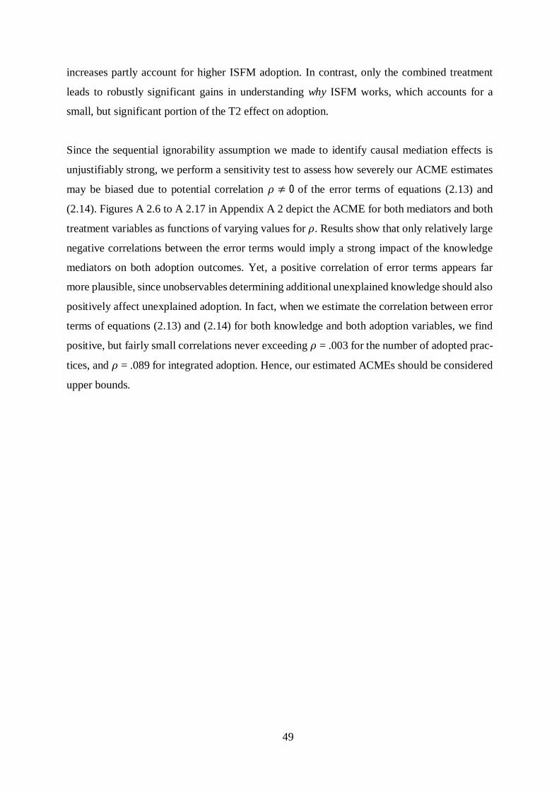
2.6 Discussion and conclusion ........................................................................................ 52Appendix A 2 ................................................................................................................. 56Appendix B 2 .................................................................................................................. 68
3. Does Integrated Soil Fertility Management increase returns to land and labor?Plot-level evidence from Ethiopia ............................................................................... 71
3.1 Introduction .............................................................................................................. 723.2 The concept and implications of ISFM ...................................................................... 743.3 Materials and methods .............................................................................................. 76
3.3.1 Study area and context ...................................................................................... 763.3.2 Sampling and data collection ............................................................................ 773.3.3 Description of treatment variable ...................................................................... 783.3.4 Description of outcome variables ...................................................................... 793.3.5 Econometric framework ................................................................................... 81
3.4 Empirical results ....................................................................................................... 853.4.1 Average treatment effects in the full sample ..................................................... 853.4.2 Differential effects by agroecological zone ....................................................... 893.4.3 Robustness checks ............................................................................................ 92
3.5 Discussion and conclusion ........................................................................................ 92Appendix A 3 ................................................................................................................. 97
4. The effects of Integrated Soil Fertility Management on household welfare inEthiopia ..................................................................................................................... 114
4.1 Introduction ............................................................................................................ 1154.2 Materials and methods............................................................................................. 118
4.2.1 Study context ................................................................................................. 1184.2.2 Sampling and data .......................................................................................... 1194.2.3 Econometric framework ................................................................................. 1194.2.4 Empirical specification ................................................................................... 122
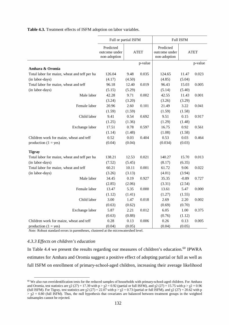
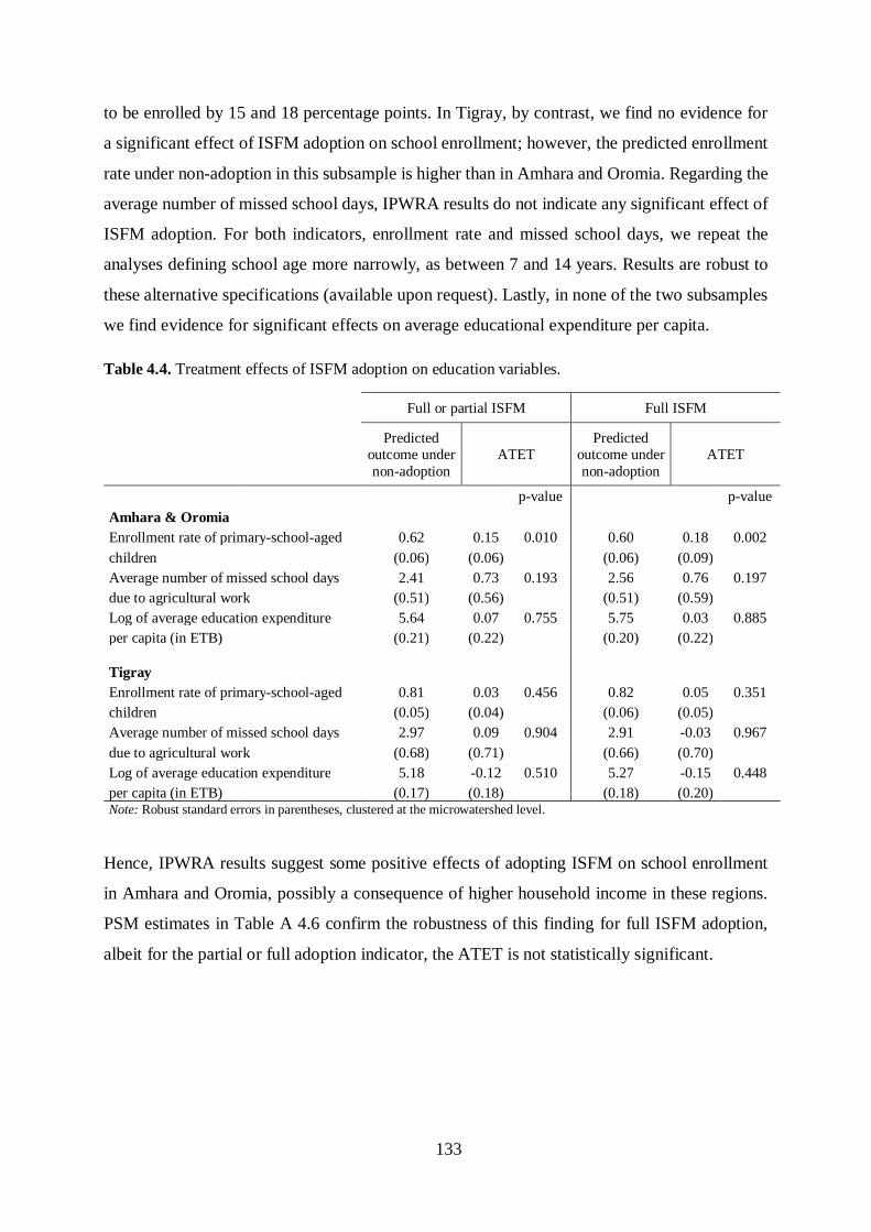
4.3 Results .................................................................................................................... 1294.3.1 Effects on income and food security ............................................................... 1294.3.2 Effects on labor demand ................................................................................. 1314.3.3 Effects on children’s education ....................................................................... 132
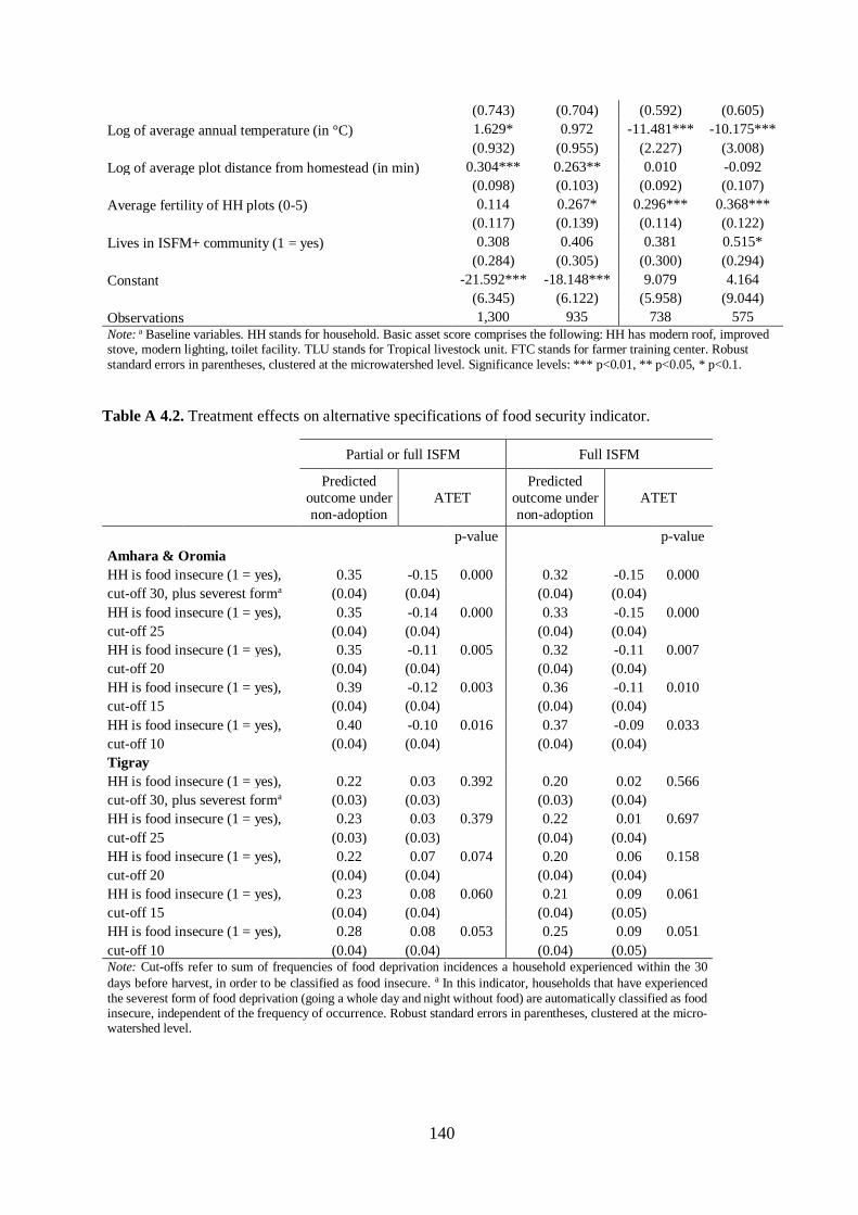
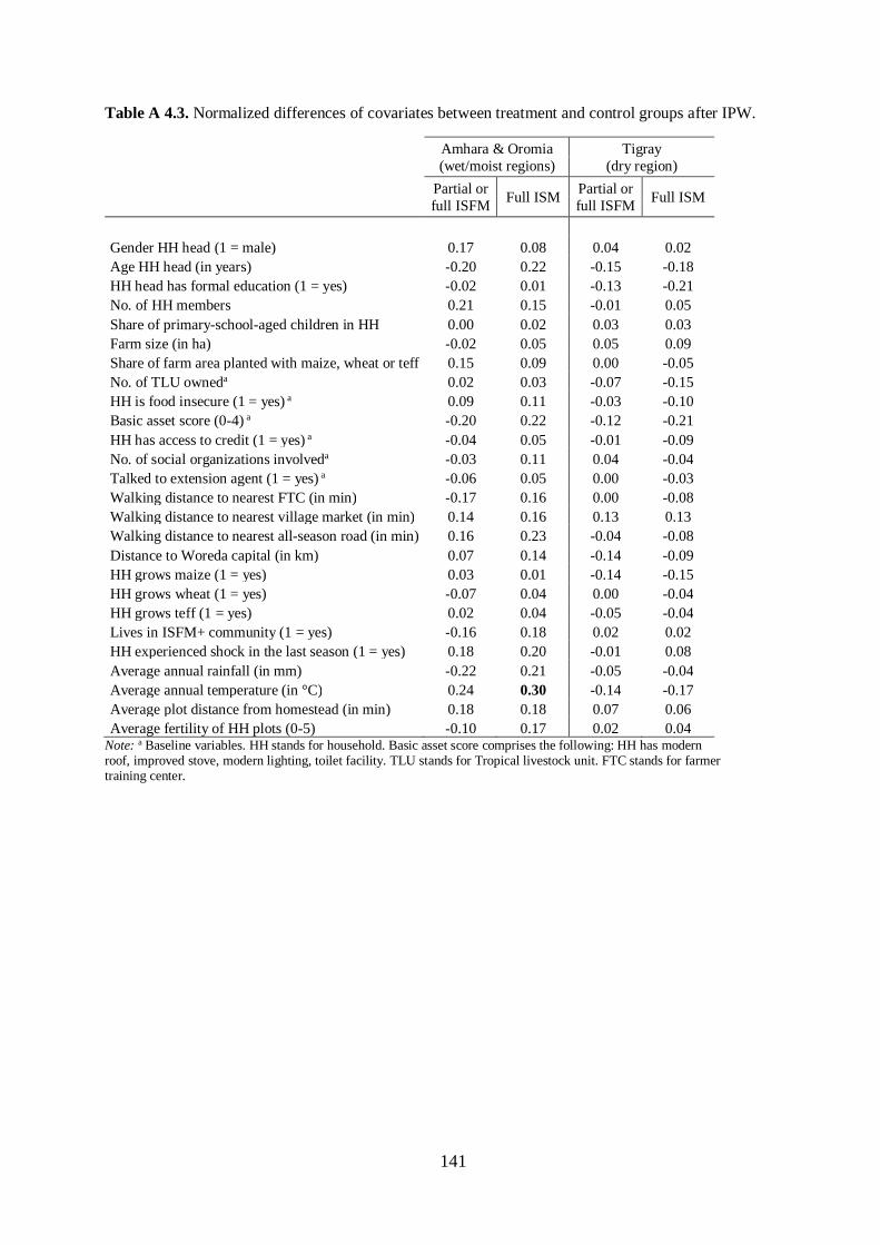
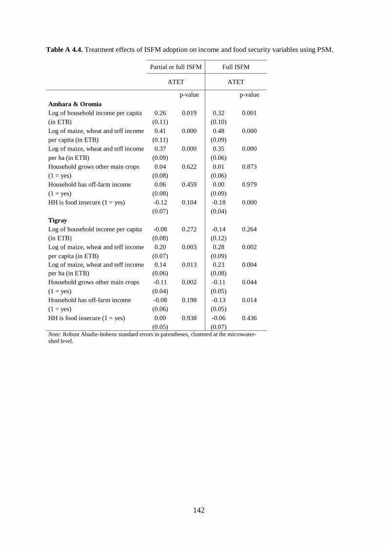
4.4 Discussion and conclusion ...................................................................................... 134Appendix A 4 ............................................................................................................... 139
5. General Conclusion................................................................................................... 1455.1 Main findings .......................................................................................................... 1465.2 Discussion............................................................................................................... 1485.3 Broader policy implications .................................................................................... 1495.4 Limitations and scope for future research ................................................................ 151
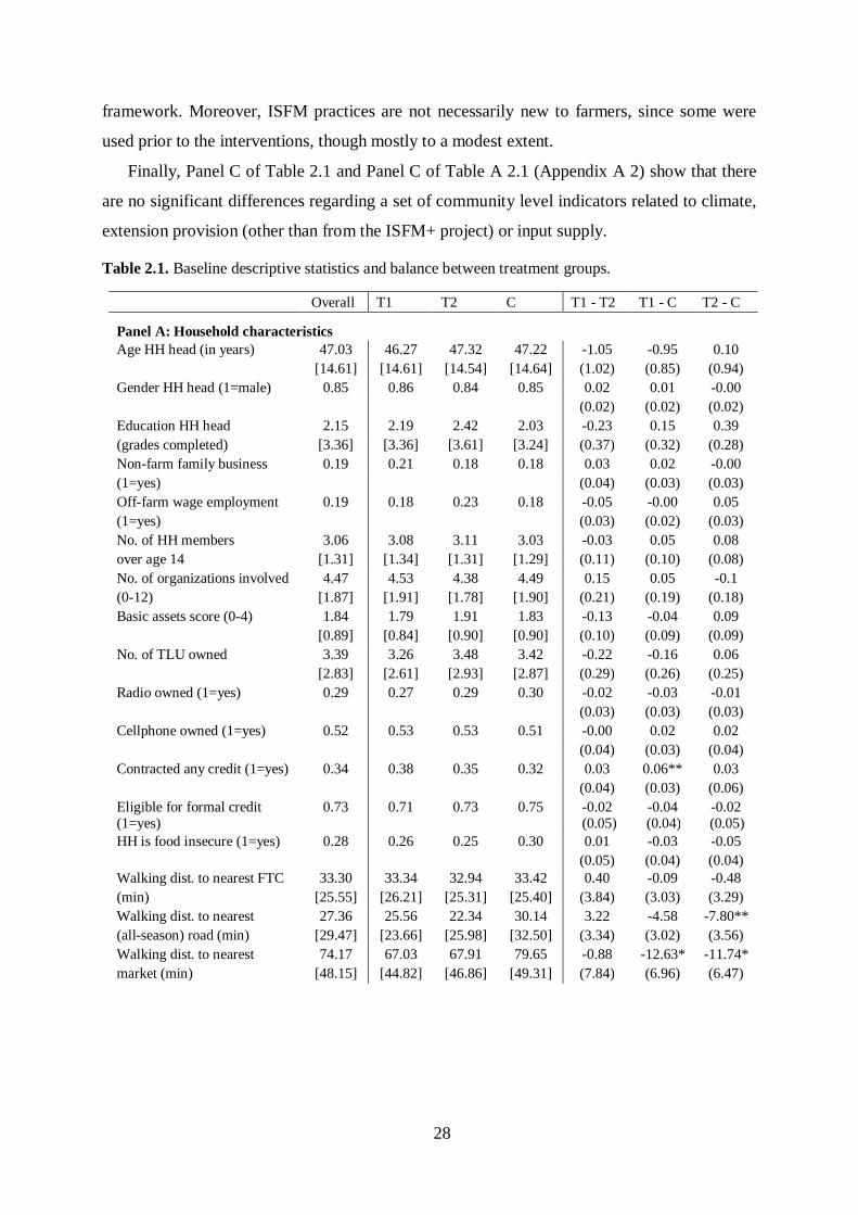
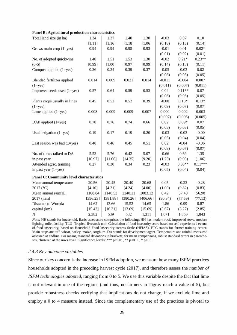
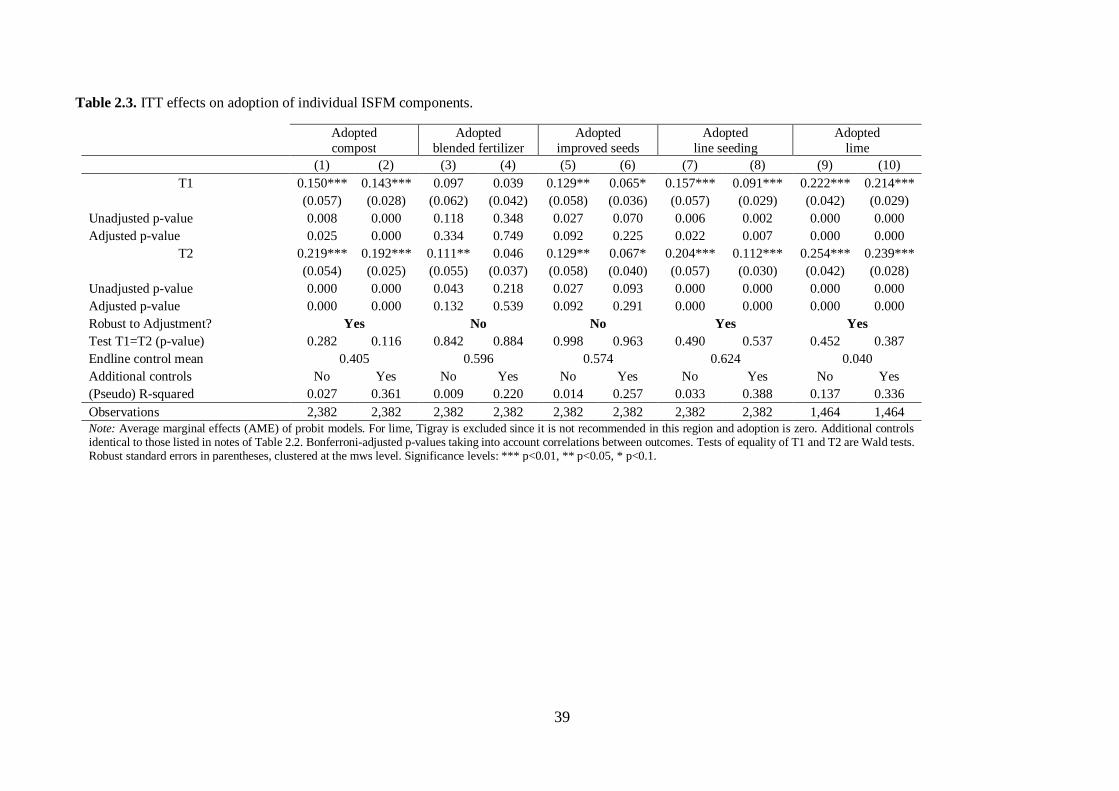
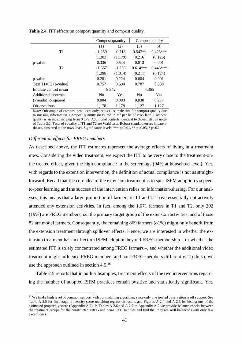
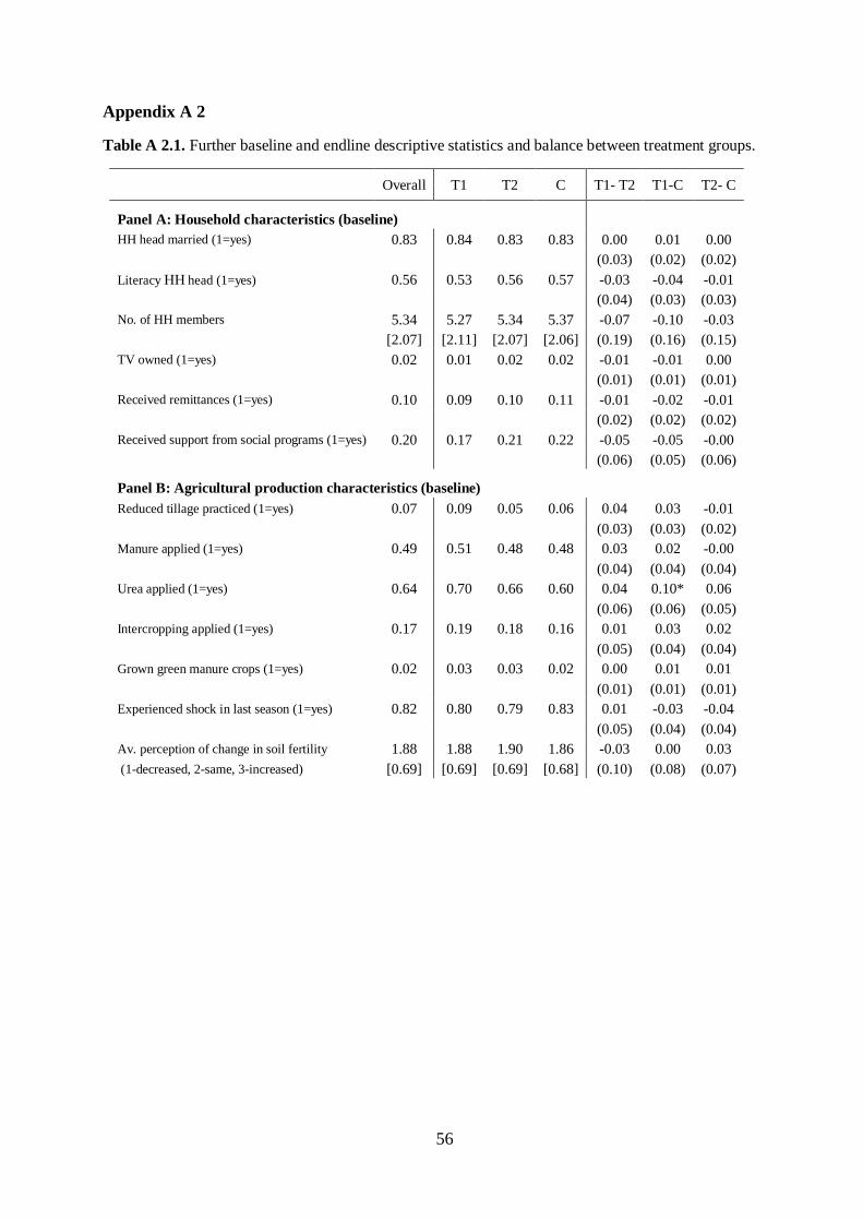
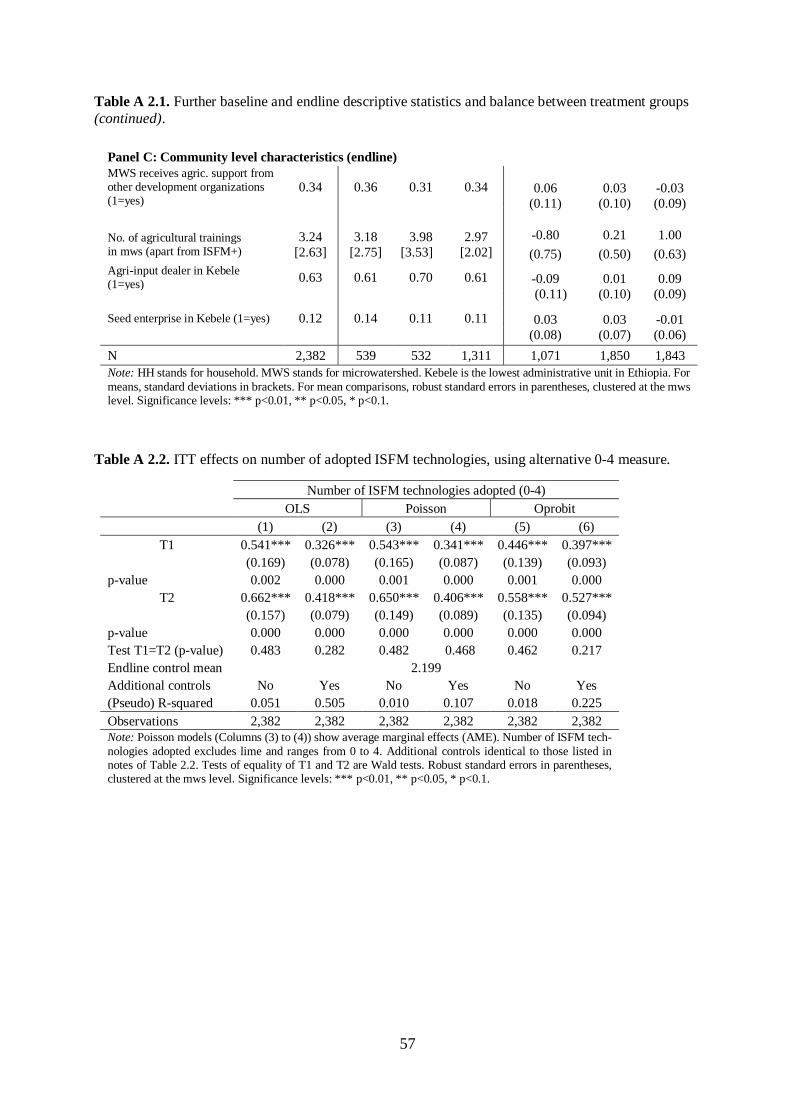
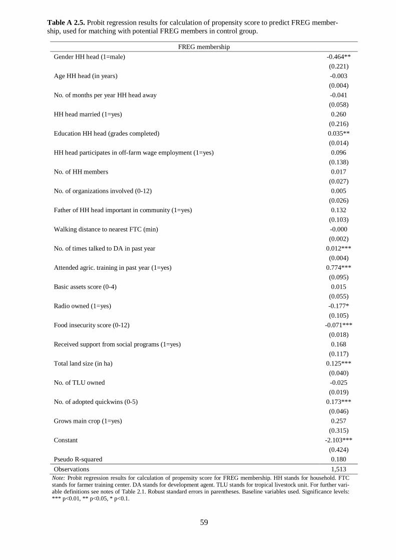
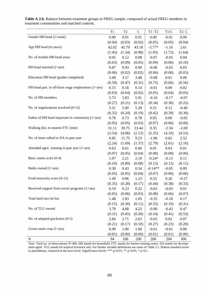
Table 2.1. Baseline descriptive statistics and balance between treatment groups. .................. 28Table 2.2. ITT effects on number of adopted ISFM technologies and integrated adoption of thefull ISFM package. ............................................................................................................... 36Table 2.3. ITT effects on adoption of individual ISFM components. .................................... 39Table 2.4. ITT effects on compost quantity and compost quality. ......................................... 41Table 2.5. ITT effects on number of adopted ISFM technologies and integrated adoption of thefull ISFM package, FREG- and non-FREG samples separately. ............................................ 44Table 2.6. ITT effects on different knowledge outcomes. ..................................................... 45Table 2.7. ITT effects on different knowledge outcomes, FREG- and non-FREG samplesseparately. ............................................................................................................................ 47Table 2.8. ITT and knowledge effects on number of adopted ISFM technologies and integratedadoption of the full ISFM package, ADE of treatments and ACME of overall, principles andhow-to knowledge as mediating variables. ............................................................................ 50Table A 2.1. Further baseline and endline descriptive statistics and balance between treatmentgroups. ................................................................................................................................. 56Table A 2.2. ITT effects on number of adopted ISFM technologies, using alternative 0-4measure. ............................................................................................................................... 57Table A 2.3. ITT effects on integrated adoption of the full ISFM package, using alternativemeasures............................................................................................................................... 58Table A 2.4. ITT effects on number of adopted ISFM technologies and integrated adoption ofthe full ISFM package, excluding model farmers. ................................................................. 58Table A 2.5. Probit regression results for calculation of propensity score to predict FREGmembership, used for matching with potential FREG members in control group. ................. 59Table A 2.6. Balance between treatment groups in FREG sample, composed of actual FREGmembers in treatment communities and matched controls. .................................................... 60Table A 2.7. Balance between treatment groups in non-FREG sample, composed of actual non-FREG farmers in treatment communities and matched controls. ........................................... 61
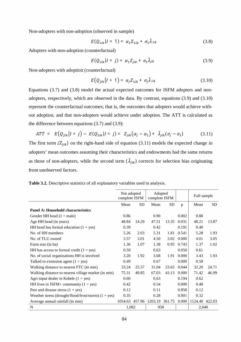
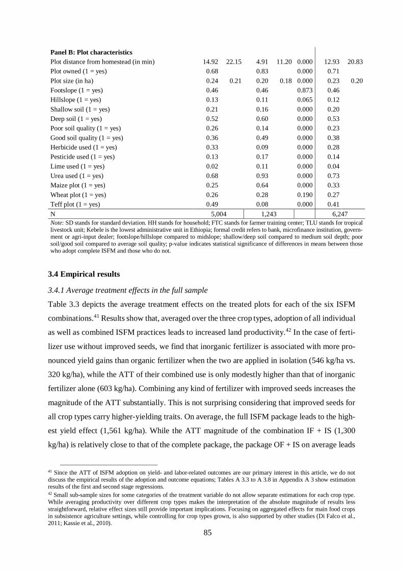
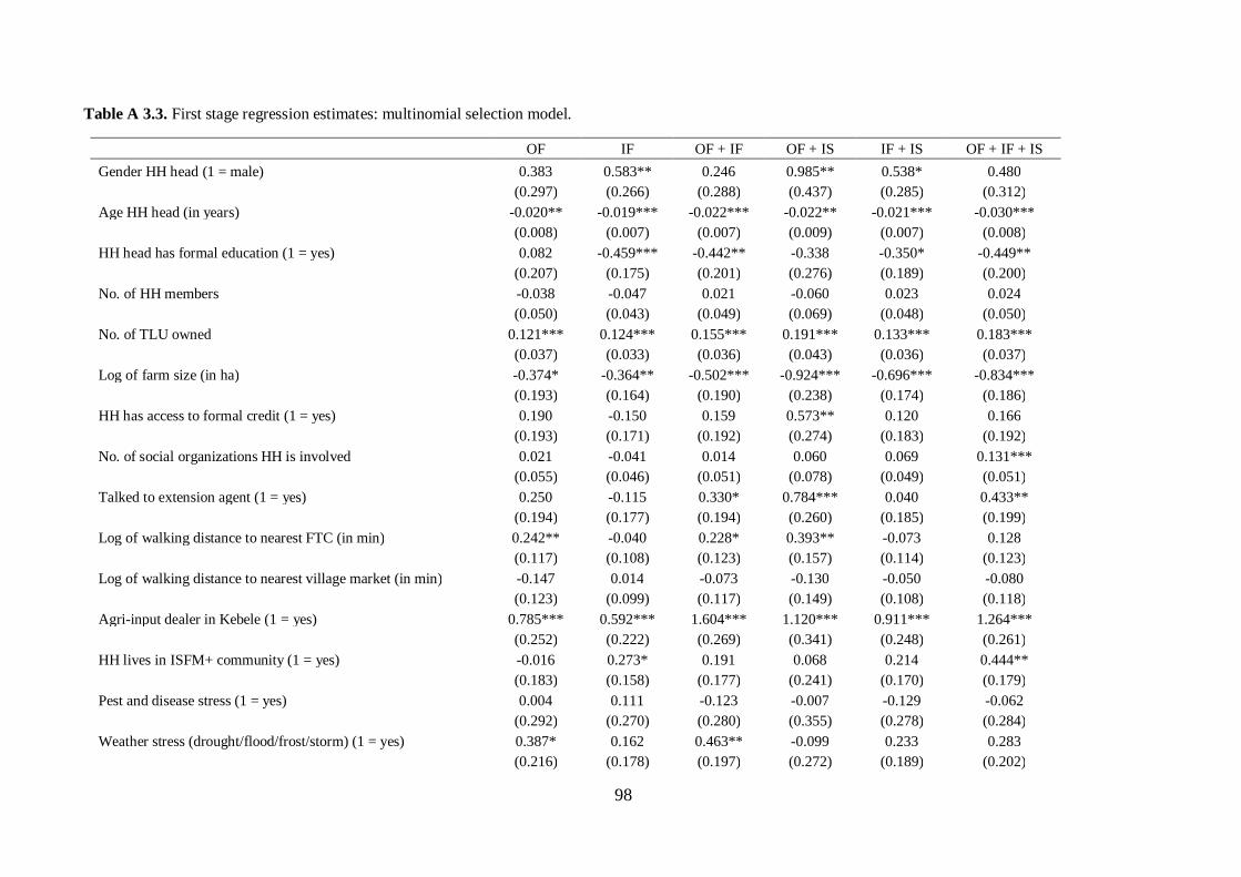
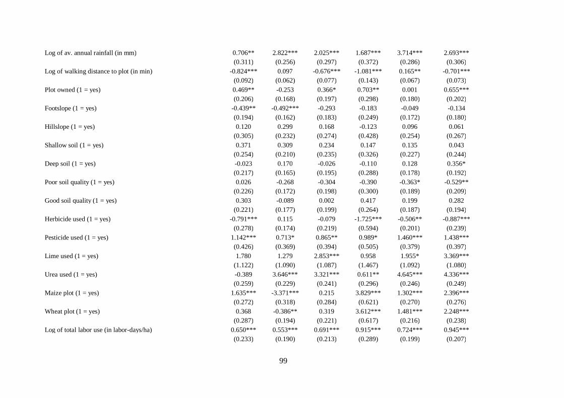
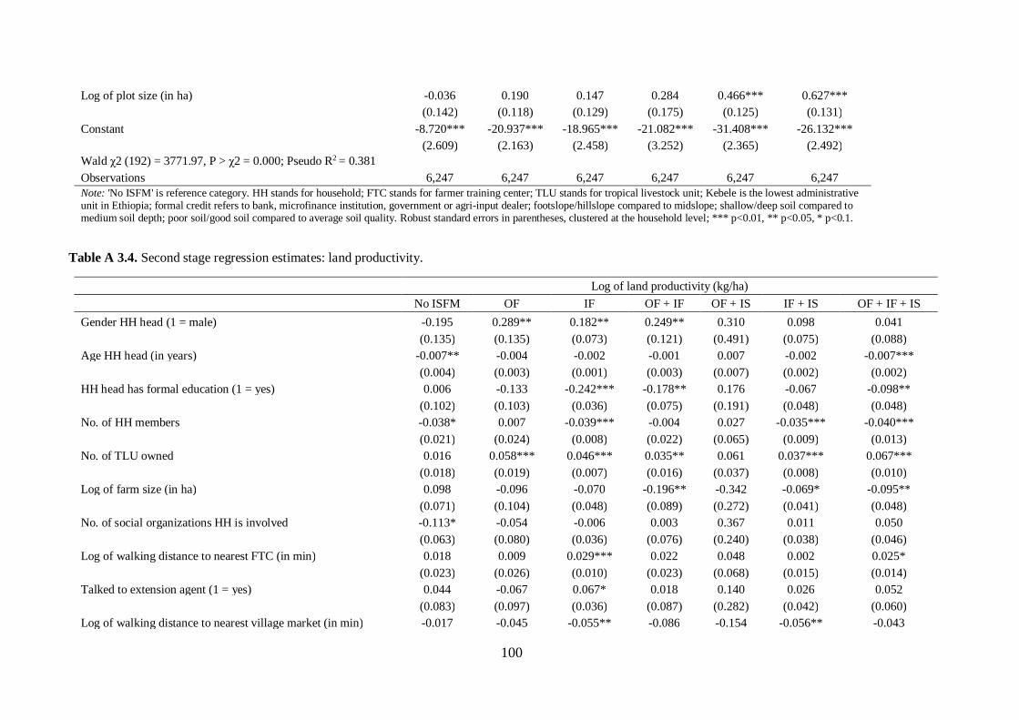
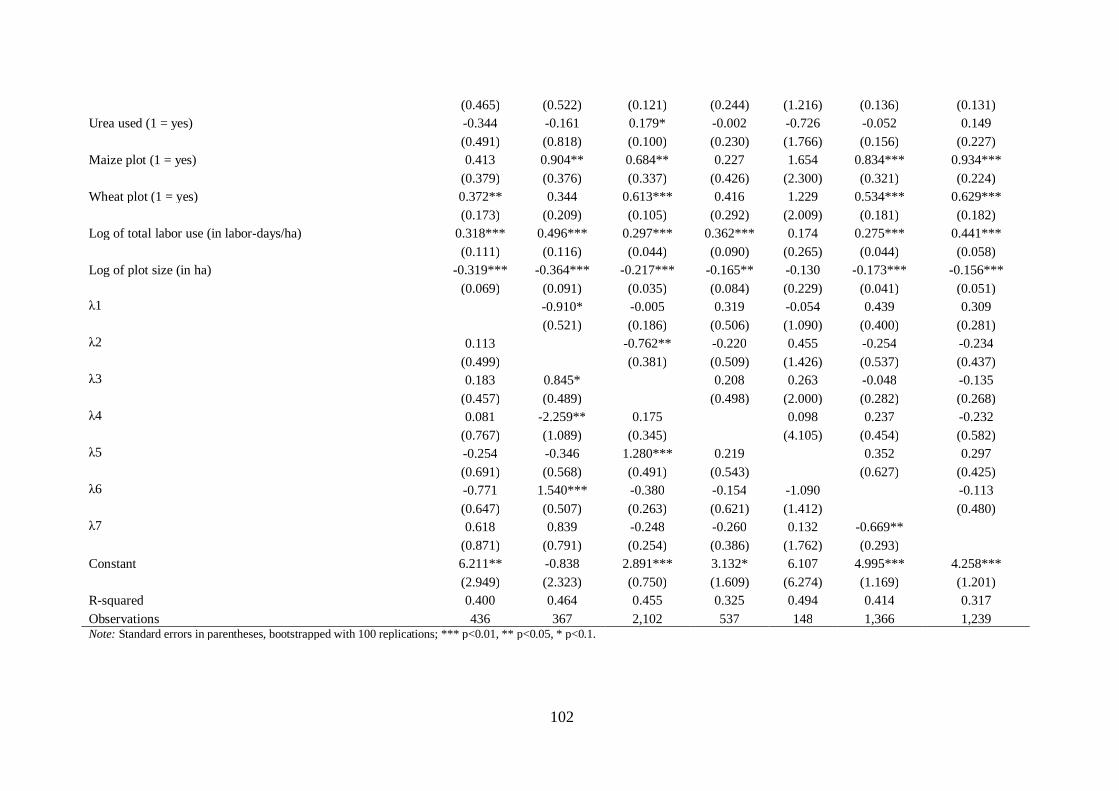
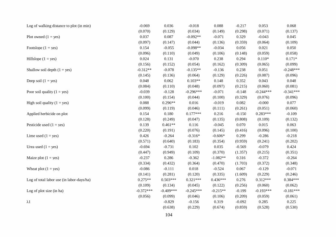
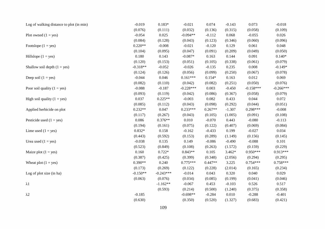
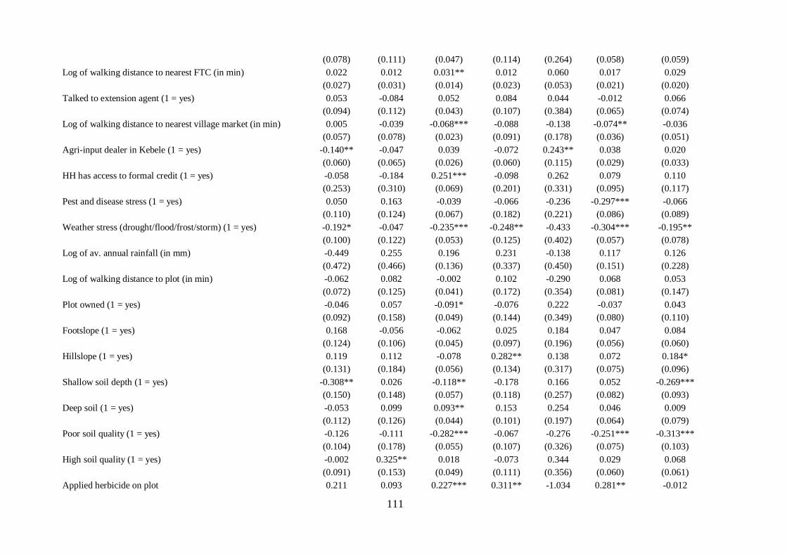
Table 3.1. Descriptive statistics of all outcome variables. ..................................................... 80Table 3.2. Descriptive statistics of all explanatory variables used in analysis. ....................... 84Table 3.3. Average ISFM adoption effects on the treated plots. ............................................ 87Table 3.4. Average ISFM adoption effects on the treated plots by agroecological zone. ....... 91Table A 3.1. Association between instrumental variable and selection variable (adoption ofISFM practices). ................................................................................................................... 97Table A 3.2. Associations between instrumental variable and outcome variables.................. 97Table A 3.3. First stage regression estimates: multinomial selection model. ......................... 98Table A 3.4. Second stage regression estimates: land productivity. .................................... 100Table A 3.5. Second stage regression estimates: net crop value. ......................................... 103Table A 3.6. Second stage regression estimates: labor demand. .......................................... 105Table A 3.7. Second stage regression estimates: labor productivity. ................................... 108Table A 3.8. Second stage regression estimates: returns to unpaid labor. ............................ 110
xi
Table A 3.9. Robustness check: crop type effects per agroecological zone. ........................ 113
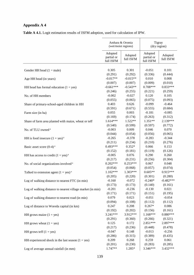
Table 4.1. Descriptive statistics of all outcome and explanatory variables used in analyses.127Table 4.2. Treatment effects of ISFM adoption on income and food security variables. ...... 130Table 4.3. Treatment effects of ISFM adoption on labor variables. ..................................... 132Table 4.4. Treatment effects of ISFM adoption on education variables. .............................. 133Table A 4.1. Logit estimation results of ISFM adoption, used for calculation of IPW. ........ 139Table A 4.2. Treatment effects on alternative specifications of food security indicator. ...... 140Table A 4.3. Normalized differences of covariates between treatment and control groups afterIPW. ................................................................................................................................... 141Table A 4.4. Treatment effects of ISFM adoption on income and food security variables usingPSM. .................................................................................................................................. 142Table A 4.5. Treatment effects of ISFM adoption on labor variables using PSM. ............... 143Table A 4.6. Treatment effects of ISFM adoption on education variables using PSM. ........ 144
List of figures
Figure 1.1. Map of Ethiopia depicting the location of the 18 study Woredas within the threeregions.................................................................................................................................. 12
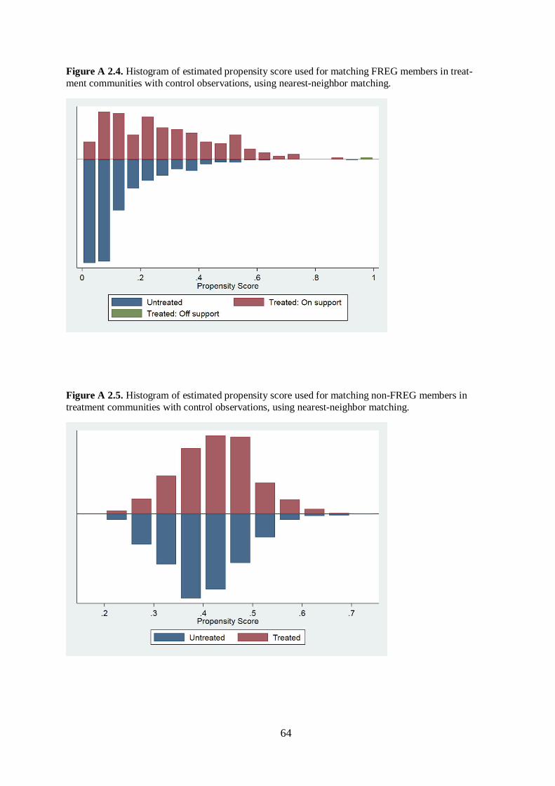
Figure 2.1. Diagrammatic illustration of the full sample. ...................................................... 24Figure A 2.1. ISFM demonstration plot for maize, next to traditional practices. ................... 62Figure A 2.2. ISFM demonstration plot for wheat, next to traditional practices. ................... 62Figure A 2.3. ISFM demonstration plot for teff, next to traditional practices. ....................... 63Figure A 2.4. Histogram of estimated propensity score used for matching FREG members intreatment communities with control observations, using nearest-neighbor matching. ............ 64Figure A 2.5. Histogram of estimated propensity score used for matching non-FREG membersin treatment communities with control observations, using nearest-neighbor matching. ........ 64Figure A 2.6. Sensitivity test ACME overall knowledge (T1), no. of adopted practices……65Figure A 2.7. Sensitivity test ACME overall knowledge (T2), no. of adopted practices….. .. 65Figure A 2.8. Sensitivity test ACME overall knowledge (T1), integr. adoption………..……65Figure A 2.9. Sensitivity test ACME overall knowledge (T2), integr. adoption……….. ....... 65Figure A 2.10. Sensitivity test ACME prin. knowledge (T1), no. of adopted practices………66Figure A 2.11. Sensitivity test ACME prin. knowledge (T2), no. of adopted practices…… .. 66Figure A 2.12. Sensitivity test ACME prin. knowledge (T1), integr. adoption………………66Figure A 2.13. Sensitivity test ACME prin. knowledge (T2), integr. adoption…….. ............ 66Figure A 2.14. Sensitivity test ACME how-to knowledge (T1), no. of adopted practices…..67Figure A 2.15. Sensitivity test ACME how-to knowledge (T2), no. of adopted practices. ..... 67Figure A 2.16. Sensitivity test ACME how-to knowledge (T1), integr. Adoption.….………67Figure A 2.17. Sensitivity test ACME how-to knowledge (T2), integr. adoption…………….67
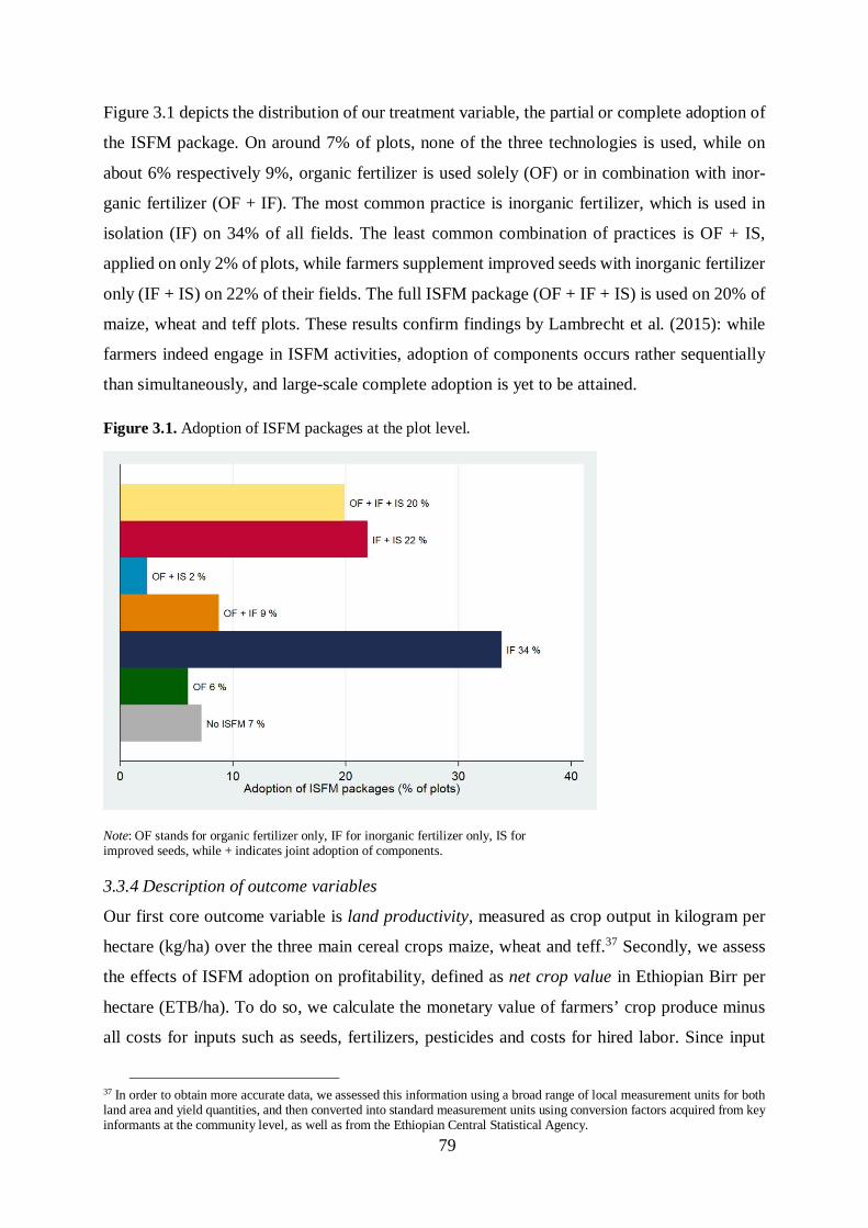
Figure 3.1. Adoption of ISFM packages at the plot level. ..................................................... 79
xii
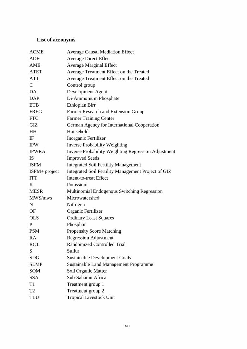
List of acronyms
ACME Average Causal Mediation EffectADE Average Direct EffectAME Average Marginal EffectATET Average Treatment Effect on the TreatedATT Average Treatment Effect on the TreatedC Control groupDA Development AgentDAP Di-Ammonium PhosphateETB Ethiopian BirrFREG Farmer Research and Extension GroupFTC Farmer Training CenterGIZ German Agency for International CooperationHH HouseholdIF Inorganic FertilizerIPW Inverse Probability WeightingIPWRA Inverse Probability Weighting Regression AdjustmentIS Improved SeedsISFM Integrated Soil Fertility ManagementISFM+ project Integrated Soil Fertility Management Project of GIZITT Intent-to-treat EffectK PotassiumMESR Multinomial Endogenous Switching RegressionMWS/mws MicrowatershedN NitrogenOF Organic FertilizerOLS Ordinary Least SquaresP PhosphorPSM Propensity Score MatchingRA Regression AdjustmentRCT Randomized Controlled TrialS SulfurSDG Sustainable Development GoalsSLMP Sustainable Land Management ProgrammeSOM Soil Organic MatterSSA Sub-Saharan AfricaT1 Treatment group 1T2 Treatment group 2TLU Tropical Livestock Unit
1
1. General introduction
1.1 Background and research objectives
1.1.1 The need for a sustainable intensification of agriculture
The rising demand for agricultural commodities, coupled with an increasing global competition
for land between food production and other economic activities, put an enormous pressure on
food systems and the natural resource base. Agricultural expansion and related land use change
are recognized as the most important drivers of land degradation as well as biodiversity loss,
which has occurred at an unprecedented rate during the past 50 years (IPBES, 2019). Most
likely, climate change will exacerbate this process by adversely affecting terrestrial ecosystems
and further contributing to land degradation. At the same time, climate change is intensified
itself by massive global land use change through the release of greenhouse gas emissions
(IPCC, 2019). In addition to environmental sustainability, achieving stable food security re-
mains a major global challenge. After decades of steady decrease, the prevalence of hunger has
stagnated in recent years the at a level of around 11 percent of the global population being
undernourished (FAO, 2019). The ‘twin-challenge’ of eradicating hunger while preserving and
restoring the natural resource base is addressed in the framework of the Sustainable Develop-
ment Goals (SDGs). Through SDG 2, the global community commits to “end hunger, achieve
food security and […] promote sustainable agriculture” by 2030, while SDG 15 states to “pro-
tect, restore and promote sustainable use of terrestrial ecosystems, sustainably manage forests
[…] halt and reverse land degradation and halt biodiversity loss” (UN, 2015).
This ‘twin-challenge’ is particularly urgent in Sub-Saharan Africa (SSA), which is currently
experiencing a rise in the prevalence of undernourishment, estimated to affect around 23 per-
cent of the population (FAO, 2019). The region also faces the most rapid population growth,
with its population projected to at least double by 2050 (UN, 2019). Currently, agricultural
production growth cannot keep pace with these demographic trends. For example, the demand
for cereals will approximately triple until the mid of this century, whereas present consumption
levels already depend to a considerable extent on imports (Van Ittersum et al., 2016). Climate
change is likely to put agricultural systems in SSA under additional strain. Though spatial ef-
fects are not entirely clear yet, most evidence suggests that increased climate variability and
climate change will have particularly adverse effects in regions that are already prone to food
insecurity, including large parts of SSA (Wheeler & von Braun, 2013).
2
In past decades, much of the agricultural production growth in SSA happened through an
expansion in area, rather than an increase in productivity. Though progress can be noted in
some areas within SSA, yields still lag substantially behind global averages, and also behind
estimated averages for maximum attainable yields in a given region (FAO, 2020; Mueller et al.,
2012). To a considerable extent, this ‘yield gap’ can be attributed to the slow adoption of agri-
cultural innovations in SSA. Whereas in Asia and Latin America the development and use of
improved technologies such as fertilizers, new crop varieties and irrigation has contributed to
substantial productivity gains, Africa is lagging behind its ‘Green Revolution’. Recently, exter-
nal input application is accelerating gradually, but use and intensities are generally still far be-
low optimal levels (Sheahan & Barrett, 2017). An average farmer outside of SSA, for example,
applies almost 15 times more fertilizer per hectare than the average SSA farmer (Vanlauwe et
al., 2014).
Given the comparatively low rates of input use, farmers in SSA depend decisively on their
soils and the nutrients provided by them. Some parts of SSA have favorable climate and soil
conditions. Yet, for a long time, agricultural systems have been largely based on nutrient min-
ing, resulting in a steady decline of nutrient stocks, soil carbon, and deteriorating soil health.
An estimated 65% of SSA’s land area can be classified as degraded, i.e. characterized by phys-
ical, chemical and biological deterioration, including top soil erosion, compaction, loss of or-
ganic matter, salinization, acidification, and consequently, low soil fertility (Zingore et al.,
2015). Soils are particularly nutrient-depleted in densely populated areas, where regeneration
through fallow periods is not viable and nutrient recycling through organic and inorganic ferti-
lizer application is insufficient (Vanlauwe et al., 2014; Zingore et al., 2015). Poor soil status is
often closely intertwined with rural poverty via self-reinforcing negative feedback loops (Tit-
tonell & Giller, 2013). Research shows that poverty prevents many smallholders from investing
in an improvement of their soils’ fertility (Barrett & Bevis, 2015). As land and labor productiv-
ity decrease with deteriorating soils, rural dwellers typically try to cope with this by farming
their land even more intensively, or making increased use of nearby natural resources, which
further aggravates soil degradation and, over time, poverty (Barbier & Hochard, 2018).
Large parts of the scientific community agree that these intertwined challenges of environmen-
tal degradation, climate change, food insecurity and rural poverty need to be tackled conjointly
by a sustainable intensification of agriculture. Sustainable intensification refers to increasing
agricultural production on the same area of land, while at the same time, reducing its negative
growth should not happen by further expanding the agricultural area, but by increasing yields
on underperforming lands – which are often managed by small-scale farmers in developing
countries (Garnett et al., 2013; Mueller et al., 2012; Pretty, 2018; Tilman et al., 2011). However,
the concept of sustainable intensification does not provide a ‘one-size-fits-all’ solution. It rather
describes a goal, while recognizing that the means are context-, region- and time-specific. Ac-
knowledging the large heterogeneity of smallholder types and conditions, there is also a multi-
tude of pathways towards sustainable intensification, and most likely no technology or man-
agement system will be the best solution forever (Garnett et al., 2013; Pretty, 2018; Vanlauwe
et al., 2014). Further, understanding the term ‘sustainable’ in its most commonly used sense,
agricultural systems need to be viable from an environmental, economic, as well as a social
perspective. Thus, apart from preserving land and natural resources, sustainable agriculture
needs to provide economic benefits to farmers while being socially inclusive, i.e. acceptable
and feasible for a large number of different smallholders.
1.1.2 Integrated Soil Fertility Management as means to sustainable intensification
Substantial evidence on yield gaps in SSA suggests that there is much potential to increase
agricultural productivity by restoring degraded soils and replenishing nutrient stocks (Mueller
et al., 2012; Sanchez et al., 2009; Tittonell & Giller, 2013; Vanlauwe et al., 2014). There is a
general consensus that much higher levels of inorganic fertilizer are needed to catalyze sustain-
able intensification in SSA, as well enhanced use of plant genetic resources (Jayne et al., 2019).
In this regard, two crucial elements of sustainable intensification are the increase of resource
use efficiency and the substitution of technologies (Foley et al., 2011; Pretty, 2018). Increasing
efficiency refers to making better use of on-farm resources and external inputs, thus, allowing
less waste of valuable nutrients and escape of agrochemicals across farm boundaries. For ex-
ample, efficiency gains can accrue from precise dosing and targeting of fertilizers, recycling
on-farm organic resources, and from the simultaneous use of organic and inorganic nutrient
sources due to synergistic effects. Substitution refers to the replacement of less suited technol-
ogies by improved ones. For instance, traditional seeds may be substituted by improved crop
varieties that better convert nutrients into biomass, are more drought-tolerant and locally
adapted to increase pest and disease tolerance. Another example are standard blanket fertilizers,
which are increasingly replaced by inorganic fertilizers that address area-specific nutrient con-
straints in order to improve crop response (Pretty, 2018; Vanlauwe et al., 2015).
The ‘Integrated Soil Fertility Management’ (ISFM) approach subsumes these key elements of
sustainable intensification (Jayne et al., 2019), and is increasingly promoted by governments
4
and international donors across SSA. ISFM is a ‘system technology’ that aims at enhancing soil
fertility and agricultural productivity through adequate nutrient and input management while
maximizing their use efficiency. The core of this technology package is the integrated use of
improved seeds with organic and inorganic fertilizers, adapted to local conditions (Vanlauwe
et al., 2010). Depending on the local context, core ISFM technologies should be complemented
by other practices such as cereal-legume intercropping, agroforestry, reduced tillage or lime
application to correct soil acidity (Vanlauwe et al., 2015). And lastly, ISFM comprises a general
improvement of agronomic techniques, such as timely weeding, line seeding or microdosing of
fertilizers and other inputs.
Higher-yielding crop varieties are seen as main drivers of an ‘African Green Revolution’,
because they can improve agricultural output per area and increase farmers’ resilience to shocks
(Sanchez et al., 2009; Takahashi, Muraoka, et al., 2019). Yet, their potential can only be fully
realized when matched with adequate soil management strategies and nutrient application
(Sanchez, 2002). Organic and inorganic fertilizers comprise different compositions of nutrients
and/or carbon and hence, address soil fertility constraints in a complementary manner. Further,
the soil’s responsiveness to mineral fertilizers is often considerably inhibited by low levels of
soil organic matter (SOM) and soil moisture (Marenya & Barrett, 2009; Place et al., 2003; Van-
lauwe et al., 2010). Organic fertilizer provides additional nutrients, and can, over time, help to
improve SOM levels and soil moisture, which both regulate the solubility and thus, the availa-
bility of added nutrients for crop uptake (Marenya & Barrett, 2009). Efficient use of inorganic
fertilizers, in turn, enhances on-farm biomass production of both crops and residues, and con-
sequently, the availability of organic materials for resource recycling (Vanlauwe et al., 2013).
Summing up, ISFM builds on a combination of methods from organic and conventional agri-
culture. Even though some proponents advocate for a pure organic approach as pathway to-
wards truly sustainable agriculture, recent evidence suggests that it will probably be unable to
raise food production sufficiently (Keating et al., 2013; Meemken & Qaim, 2018). Though or-
ganic has shown to be less polluting than conventional agriculture when measured per unit of
land, this is not true when measured per unit of output due to lower average yields on a given
area of land (Meemken & Qaim, 2018). Considering the imperative of not further expanding
the agricultural frontier and the urgent need to enhance food security, a well-managed mix of
organic farming practices and moderate levels of agrochemicals, as proposed by ISFM, seems
the most viable approach towards a sustainable intensification of agriculture in SSA.
5
1.1.3 Enhancing the use of Integrated Soil Fertility Management
Against this background, a crucial question is how to enhance the use of ISFM among small-
scale farmers. Two key points are identified in the literature. Firstly, adoption of technologies
requires an enabling environment. In many parts of SSA, the increasing fragmentation of farms
coupled with insecure land tenure makes investments in new technologies unattractive and un-
viable for farmers, while inadequate infrastructure impedes access to capital, seed and input
markets. Hence, restructuring and strengthening infrastructure and institutions are indispensa-
ble to promote sustainable soil management practices (Foley et al., 2011; Jayne et al., 2019;
Vanlauwe et al., 2014). Another decisive element with respect to an enabling environment is
how knowledge and innovation systems need to be designed, which is especially relevant for
relatively complex system technologies. Since ISFM is a flexible concept, it requires at least a
basic understanding of biological processes, and the adaptation of practices to local agroeco-
logical conditions. In this regard, Pretty (2018) emphasizes the need for new ‘knowledge econ-
omies’ built on social capital, in which knowledge is best created and spread locally and col-
lectively.
In recent decades, governments across SSA refocused on the agricultural sector, including
substantial investments and a restructuring of extension systems (Berhane et al., 2018; Ragasa
& Niu, 2017; Swanson, 2008). The core of extension is the transfer of agricultural knowledge
to farmers. Yet, in the past, most extension systems in SSA showed limited success in spurring
large-scale adoption of agricultural innovations. In fact, shortcomings like high bureaucratic
burden, high financial costs and weak institutions often led to an undersupply of trainings, lim-
ited geographic coverage and the exclusion of marginalized farmers (Anderson & Feder, 2007).
In many countries, extension now follows a more decentralized and participatory approach,
involving farmers as active stakeholders in the technology innovation and transfer process ra-
ther than perceiving them as mere recipients. In these ‘farmer-to-farmer’ models, extension
agents train only few ‘model’ or ‘contact farmers’ who pass on their knowledge to other farm-
ers, often organized in groups, where technologies should be further developed and adapted to
local needs in a participatory and experiential way. From there, information should eventually
reach the broader rural population via information sharing (Swanson, 2008; Takahashi, Mu-
raoka, et al., 2019). In line with the sustainable intensification paradigm, these developments
often go along with a change from a pure output-growth to a more holistic perspective, promot-
ing technologies that achieve productivity increases and sustainable use of natural resources at
the same time (Swanson, 2008). In addition, extension systems increasingly incorporate non-
traditional ways of spreading agricultural information, in particular via media and other
6
information and communication technologies, such as mobile phones, radio programs or videos
(Aker, 2011). This leads to the first overall research objective of this dissertation:
(1) To assess the potential of farmer-to-farmer and non-traditional forms of extension to
enhance knowledge and adoption of ISFM as a pathway to sustainable intensification.
A second main determinant of adoption are the incentives farmers face. As Vanlauwe et al.
(2014: 17) state, smallholders’ engagement will ultimately be determined by the profitability
of a technology package, while “its [environmental] sustainability will not necessarily be their
immediate concern”. This holds even more true considering that small-scale farmers are often
present-biased, as poverty impedes investing in strategies that might only pay off in the longer
run, or being overly concerned with environmental issues (Jayne et al., 2019). Farmers are
probably more likely to adopt a technology package that offers (immediate) positive economic
returns, including gains in productivity, profitability and overall welfare. In particular, system
technologies such as ISFM typically go along with additional labor as well as capital input, so
that farmers will likely adopt only if these additional investments pay off (Jayne et al., 2019).
Consequently, the second broad research objective of this dissertation is:
(2) To assess the productivity and welfare implications of adopting ISFM practices at the
plot and household level.
1.2 Research gaps and questions
1.2.1 Research objective 1
The first essay of this dissertation addresses the role of extension in fostering knowledge and
adoption of complex agricultural technologies such as ISFM. A considerable body of literature
concludes that providing training to farmers enhances their knowledge and adoption of tech-
nologies (e.g. De Brauw et al., 2018; Feder et al., 2004; Fisher et al., 2018; Godtland et al.,
2004; Kondylis et al., 2017; Nakano et al., 2018; Ogutu et al., 2018; Takahashi, Mano, et al.,
2019). Yet, evidence is less clear when it comes to diffusion to peers, a crucial determinant of
success of farmer-to-farmer extension. While a series of studies finds positive effects of training
some farmers on their neighbors’ knowledge or behavior (Fisher et al., 2018; Nakano et al.,
2018; Takahashi, Mano, et al., 2019), others suggest that neither knowledge (Feder et al., 2004;
Rola et al., 2002; Tripp et al., 2005) nor technology diffusion (Kondylis et al., 2017; Van den
Berg & Jiggins, 2007) to peers takes place. Niu and Ragasa (2018) observe that while
knowledge transmission from extension agents to lead farmers and from there to other farmers
occurs, important pieces of information get lost along the way due to selective attention of both
7
communicators and recipients. Yet, other research suggests that incomplete information trans-
mission can be counterbalanced by reminders of commonly neglected information (Hanna et
al., 2014). Overall, the available evidence shows that farmer-to-farmer technology dissemina-
tion is a multifaceted process that does not occur automatically. It is reasonable to assume that
this is particularly true in the case of system technologies, i.e. sets of technologies that should
be used in combination, where farmers have to learn about each individual practice as well as
the importance of applying them jointly. While there is an emerging strand of literature on
farmer-to-farmer extension, studies do mostly not focus on the integrated uptake of system
technologies, despite the high policy relevance. In addition, there is hardly any evidence on
how incomplete information spillovers from extension beneficiaries to their neighbors can be
counterbalanced by additional interventions. This leads to the first set of research questions of
this thesis:
(1) Does farmer-to-farmer extension and an additional intervention in form of a video in-
crease knowledge and adoption of ISFM?
(2) Do the interventions have differential effects on farmers who are actively involved in
extension activities and non-involved farmers in the same communities?
(3) Do gains in ISFM knowledge increase its adoption?
(4) Which forms of knowledge are particularly relevant?
The first essay addresses these questions by means of a randomized controlled trial (RCT) and
data from 2,382 farm households in the Ethiopian highlands. In addition to the experimental
set-up, matching techniques and a causal mediation analysis are used to answer the research
questions.
1.2.2 Research objective 2
The second and third essays focus on the effects of ISFM adoption at the plot and household
level, respectively. There is a well-established body of literature on the plot- and household-
level impacts of individual or combined uptake of a large variety of agricultural or natural re-
source management practices (e.g. Abro et al., 2017, 2018; Becerril & Abdulai, 2010; Di Falco
et al., 2011; Jaleta et al., 2016; Kassie et al., 2010; Khonje et al., 2015, 2018; Manda et al.,
2016; Noltze et al., 2013; Takahashi & Barrett, 2014; just to mention a few); some of which
analyze technology combinations that can be classified as ISFM, such as intercropping, conser-
vation tillage or improved seeds (Arslan et al., 2015; Kassie et al., 2015; Teklewold et al., 2013).
However, relatively few studies using micro-level data look into the combined use of organic
and inorganic fertilizers with improved seeds, the core ISFM technologies, and those that exist
8
(Adolwa et al., 2019; Wainaina et al., 2018) only estimate effects on productivity, crop or
household income. Yet, as concluded in a recent review article by Takahashi, Muraoka, et al.
(2019), more evidence on ISFM beyond these traditional yield and income effects is needed.
This is particularly important since ISFM usually goes along with substantial investments of
capital and labor for the purchase, preparation, transportation and application of inputs. More-
over, much of the evidence on the yield-enhancing effects of ISFM stems from well-managed
trial fields rather than plots managed by ‘regular’ smallholders. Since ISFM is considered
knowledge- and management-intensive, effects achieved by the latter might differ from those
achieved under best agricultural practices on trial plots (Jayne et al., 2019). Hence, in order to
draw a more comprehensive picture on the impacts of ISFM in resource-constrained small-
holder systems, evidence on the profitability of additional resource investments is required. The
second article of the thesis addresses this research gap with the following question:
(5) What are the plot-level effects of ISFM adoption on land productivity and net crop
value, as well as on labor demand, labor productivity and financial returns to labor?
More precisely, the paper focusses on the effects of organic fertilizer, inorganic fertilizer, im-
proved crop varieties and combinations thereof on 6,247 wheat, maize and teff1 plots managed
by 2,040 Ethiopian farm households. The study distinguishes between two different agroeco-
logical zones, and uses a multinomial endogenous switching model to tackle issues with self-
selection.
Lastly, it is important to assess the broader implications of adopting a capital- and labor-inten-
sive system technology at the household level. Since farm households commonly diversify their
livelihoods between different agricultural and non-agricultural economic activities, adopting
ISFM for some crops might imply reallocation effects of household resources (in particular
labor), as suggested by Takahashi and Barrett (2014) for example. Hence, net implications for
a household are not clear, even if ISFM goes along with productivity increases. For instance,
household food security can be influenced by both farm and off-farm income (Babatunde &
Qaim, 2010). Hence, while agricultural productivity gains associated with a technology can
positively influence food security, this effect might be muted if technology adoption withdraws
resources from other economic activities. Another issue of concern are possible effects on chil-
dren’s education, which are hardly addressed in studies on technology adoption (with the
1 Teff is a small cereal grain (annual grass) originating from the Northern Ethiopian highlands. While it is hardly grown inother parts of the world, it presents a major staple in Ethiopian and Eritrean diets (Baye, 2010).
9
exception of Takahashi & Barrett, 2014). On the one hand, increased demand for household
labor may increase children’s work burden, with potential negative effects for their education.
On the other hand, income gains may induce higher investments in human capital formation
and thus, positive effects on children’s education. In order to create more evidence on welfare
effects at the household level related to ISFM, the third article of this dissertation focusses on
the following:
(6) What are the effects of ISFM adoption on crop, household and off-farm income, as well
as on food security, labor demand and children’s education?
This essay uses data from 2,059 maize, wheat and teff growing households in two agroecolog-
ical zones in Ethiopia, and distinguishes between a rather lax and a stricter definition of ISFM.
The inverse probability weighting regression adjustment method is used, and propensity score
matching as robustness check.
1.3 Study context
1.3.1 Agriculture in Ethiopia
The data used in this dissertation come from Ethiopia. With around 108 million inhabitants,
Ethiopia has the second largest population in Africa, which continues to grow by 2.6% annually
(CIA, 2020). Despite considerable economic growth of around 10% annually in recent years,
one quarter of the population still lives below the national poverty line, while over 20% of the
population are undernourished and 38% of children under age five suffer from stunting (FAO,
2020). Although services have recently surpassed agriculture in terms of GDP share, the sector
remains of tremendous importance, accounting for over 35% of the country’s GDP and being
the major income source for around three fourths of the population (CIA, 2020). Three cereal
crops – maize, wheat and teff – account for 56% of the country’s cultivated area and present
the main staples in rural diets (CSA, 2019). Despite the importance of the sector and substantial
output growth in recent years, agricultural yields remain comparatively low, with average cereal
yields below 2.5 tons per hectare, and are not at par with population growth (FAO, 2020).
Land degradation and reduced soil fertility are among the most serious problems to the
Ethiopian agriculture. In 2007, 85% of the land in Ethiopia was classified as degraded to some
degree (Gebreselassie et al., 2016). Among the major causes of soil degradation are the expan-
sion of cultivated areas into marginal lands, excessive deforestation and inappropriate agricul-
tural land use practices, such as burning of rangelands, overgrazing, improper crop rotations,
insufficient fallow periods, intensive tillage or unbalanced use of mineral fertilizer
10
(Gebreselassie et al., 2016). As one of the consequences, many soils in Ethiopia lack key nutri-
ents like nitrogen, phosphorus, potassium, sulfur and zinc, in addition to suffering from water-
logging, alkalinity or acidity (Haileslassie et al., 2004).
In order to restore degraded lands, combat low agricultural productivity and prevent further
environmental deterioration, the Ethiopian government has implemented the ‘Sustainable Land
Management Programme’ (SLMP) in cooperation with international donors across large parts
of the country’s highland area (Schmidt & Tadesse, 2019). In the past three decades, the SLMP
focused on the stabilization of hillsides through physical soil conservation measures at the wa-
tershed and landscape scales. Building on these achievements, the focus has recently shifted to
an intensification of smallholder farming practices. With the 2017 Ethiopian ‘Soil Health and
Fertility Improvement Strategy’, the promotion of ISFM has become a national policy to im-
prove soil fertility and food security of a bulging population (MoANR, 2017).
These initiatives are accompanied by unprecedented investments in the agricultural exten-
sion system. Nowadays, Ethiopia counts with one of the largest public extension systems in
Africa in terms of public budget share, and has the worldwide highest extension-agent-to-
farmer ratio (Berhane et al., 2018). Further, the system has undergone a reorientation from a
centralized ‘top-down’ towards a supposedly more inclusive ‘bottom-up’ model. This decen-
tralized, participatory approach builds on model farmers and grassroots farmer groups as key
elements for technology innovation and dissemination (ATA, 2014; Berhane et al., 2018).
1.3.2 The GIZ-ISFM+ project
Against this background, in 2015 the German Agency for International Cooperation (GIZ)
launched the ‘Integrated Soil Fertility Management Project’ (ISFM+ project) in three Ethiopian
highland regions: Amhara, Oromia and Tigray.2 The project is executed under the ‘Soil Protec-
tion and Rehabilitation for Food Security’ program through the Special Initiative ‘One World
– No Hunger’ of the German Federal Ministry of Economic Cooperation and Development
(BMZ, 2015; GIZ & MoANR, 2015). The overarching goal of the ISFM+ project is to promote
the wider use of ISFM practices to improve soil fertility and productivity; and consequently, to
increase crop yields, in particular for the three main staples wheat, teff and maize. The ISFM+
project is a component of GIZ’s contribution to the SLMP3 and only operates in districts (in
2 Initially, the project was planned as a three-year program until the end of 2017. By now, it has been extended until the end of2023 and operates in a fourth region, Southern Nations, Nationalities, and Peoples' Region (SNNPR).3 Beginning of 2018, the SLMP has been replaced by the successor project named ‘Sustainable Use of Rehabilitated Land forEconomic Development’ (SURED).
11
Ethiopia called Woredas) where physical land rehabilitation measures have been successfully
introduced (GIZ & MoANR, 2015). The project works in close cooperation with the Ethiopian
Ministry for Agriculture and Natural Resources. One package of interventions concentrates on
capacity building among government agricultural advisory staff. Eventually, these local experts
are responsible for transmitting ISFM knowledge to farmers. The main target population of the
project consists of small-scale farmers in the three regions, the vast majority of which grow
staple crops for subsistence (GIZ, 2016; GIZ & MoANR, 2015).
In accordance with the national policy, model farmers present the cornerstone of the pro-
ject’s decentralized ‘participatory learning and extension approach’ for ISFM dissemination at
the farm level. Model farmers are trained by public extension agents and maintain ISFM
demonstration plots on their farms. Further, each model farmer is responsible for leading a so-
called ‘Farmer Research and Extension Group’ (FREG) in his or her community as core entity
to discuss and experiment with ISFM practices, and conducts field days to visit demonstration
sites at least twice per harvest cycle (GIZ, 2016).4 In addition, the project works with various
local stakeholders to improve supply chains for necessary inputs in all project Woredas, e.g. for
improved seeds, fertilizers or lime.
1.4 Study design and data
1.4.1 Research design and sampling
All essays of this thesis build on data from farmers in ISFM+ project Woredas. In order to
pursue the first research objective, an RCT was implemented. The experimental set-up, sam-
pling strategy and data collection were done in close cooperation with the ISFM+ project, as
well as the University of Mannheim.
The primary units of randomization are microwatersheds (mws), which are typical imple-
mentation units of natural resource related projects in Ethiopia. These are natural topographic
entities, which typically consist of an agglomeration of up to 300 households sharing a common
rainwater outlet. Target mws were selected during planning workshops in the early phase of the
project, based on the following criteria: (1) benefiting from the SLMP, (3) no/minimal previous
exposure to soil fertility interventions, and (3) targeting six Woredas in each of the three regions
Amhara, Oromia and Tigray. Out of a total sampling frame of 161 mws, 72 were randomly
selected to benefit from the ISFM+ project (treatment mws), stratified by region and Woreda.
Hence, in each of the three regions, six Woredas are targeted, and within each Woreda, four
mws were randomly selected by means of a lottery. The remaining 89 serve as control mws and
4 Further details on the project’s interventions are presented in chapter 2.
12
are located in the same Woredas. In addition to the ISFM+ interventions, in early 2017, half of
the 72 treatment mws were randomly chosen to receive a video treatment. The video treatment
consisted of a one-time video screening conducted in public venues, which primarily featured
information on why ISFM with all its components is important.5 Summing up, the RCT contains
36 mws that only received the extension treatment, 36 mws that received the extension plus the
additional video treatment, and 89 control mws.
The sampling frame for the farmer survey consisted of all households in the 161 mws, from
which approximately 15 households per mws were randomly drawn from administrative lists.
This resulted in a total sample of 2,416 households, of which 2,382 could be re-interviewed in
the follow-up data collection and thus, constitute the base sample used in this dissertation. In
addition, data on infrastructure, (extension) service provision and climate were gathered during
key informant interviews at the Woreda and mws levels in 2018. Figure 1.1 shows the location
of the study Woredas within the three regions (red framed areas).
Figure 1.1. Map of Ethiopia depicting the location of the 18 study Woredas within the three regions.
Source: GIZ-ISFM+ project Ethiopia.
5 Further details on the video treatment are presented in chapter 2.
13
1.4.2 Data
Two rounds of data were collected among the sampled households. The first round was gathered
in early 2016 as RCT baseline by researchers from the University of Mannheim. The second
wave of data collection was led by the author of this dissertation among the same rural house-
holds in the first half of 2018. All three essays mainly use data from the second wave, and make
use of baseline data as control variables (detailed descriptions in the respective chapters).
Data in both rounds were gathered using a structured questionnaire during tablet-based face-to-
face interviews with household heads or their spouses. Prior to the data collection, an intensive
ten-day enumerator training took place, with both a classroom and a field module. Question-
naire contents were thoroughly translated into the three local languages Amharic, Afaan Oromo
and Tigrigna, and pretested in several rounds. Each of the 40 enumerators was a proficient
speaker of at least one of the languages and assigned to the respective team. In each region, two
survey teams collected the data, supervised by team leaders who reported to the local survey
manager and the author as overall coordinators.
Both survey rounds contained modules on household socio-demographic characteristics,
income and assets, subjective food security level, social relationships, farming practices and
agricultural production data for the preceding cropping seasons (2015 in the baseline and 2017
in the follow-up survey), as well as exposure to agricultural extension. As far as possible, data
were assessed in the same way during follow-up, although the mode of measurement was
adapted for some variables. Moreover, the second-round-questionnaire added detailed modules
on ISFM knowledge and participation in the interventions.
1.5 Thesis outline
The remainder of this thesis is organized as follows: Chapter two presents the first essay, which
analyzes the effects of farmer-to-farmer and video-based extension on knowledge and adoption
of ISFM using an experimental research design. Chapter three presents the second essay, fo-
cusing on the effects of different ISFM practices and their combinations on land productivity,
net crop value and different labor outcomes at the plot level. Chapter four contains the third
essay, which assesses the household-level effects of ISFM adoption on income, food security,
labor and children’s education. The last section summarizes the main findings, draws overall
conclusions and puts them into the broader context of current debates on agricultural extension
and technology adoption, and also highlights some limitations of the studies and scope for fu-
ture research.
14
2. Knowledge and adoption of complex agricultural technologies –
Evidence from an extension experiment6
AbstractThe slow adoption of new agricultural technologies is an important factor in explaining persis-tent productivity deficits and poverty among smallholders in Sub-Saharan Africa. Farmer-to-farmer extension models aim to diffuse technology information from extension agents to modelfarmers and farmer group members, and then further on to other community members. Yet,only few studies investigate how to design modalities for information transmission effectively,in particular for complex and knowledge-intensive technology packages. In this study we assessthe effects of farmer-to-farmer extension and an additional video intervention on the adoptionof ‘Integrated Soil Fertility Management’ (ISFM) among 2,382 small-scale farmers in Ethiopiausing a randomized controlled trial. We find that both extension-only and extension combinedwith video induce ISFM adoption and gains in knowledge. While effects are stronger for activeparticipants, we find evidence that information diffuses to community members not activelyparticipating in the extension activities. The additional video intervention shows a significantcomplementary effect for these non-actively involved farmers, in particular when it comes tothe integrated adoption of the full technology package.
Key words: Integrated Soil Fertility Management (ISFM), system technology, technology dif-fusion, farmer-to-farmer extension, selective attention, rural development
6 This essay is co-authored by Adrien Bouguen (AB), Markus Frölich (MF) and Meike Wollni (MW). I, Denise Hörner (DH),developed and implemented the video intervention, collected the follow-up data in 2018, performed the analysis, interpretedresults and wrote the paper. MW assisted at various stages of the research; MW and MF contributed to interpreting results,writing and revising the paper. MF and AB developed the original RCT research design in collaboration with the GIZ-ISFM+project, did the initial sampling and collected the baseline data in 2016.
15
2.1 Introduction
The slow adoption of new agricultural technologies is an important factor in explaining persis-
tent productivity deficits and poverty among the rural population in developing countries, es-
pecially in Sub-Saharan Africa (SSA). Lack of technological innovation and underinvestment
in soils – an essential productive asset of smallholder farmers in SSA – is viewed as a major
cause for self-reinforcing poverty traps in rural areas (Barrett & Bevis, 2015). Recent evidence
shows that farmers delay in particular the uptake of integrated system technologies, i.e. pack-
ages of agricultural practices that should be jointly applied in order to deploy their full produc-
tivity-enhancing potential (Noltze et al., 2012; Sheahan & Barrett, 2017; Ward et al., 2018).
Integrated system technologies are typically knowledge-intensive, as they require the under-
standing of at least basic underlying biological functions and processes and the adaptation of
practices to local agri-environmental conditions (Jayne et al., 2019; Vanlauwe et al., 2015).
While information and knowledge constraints are frequently cited barriers to the adoption of
agricultural innovations in general (Aker, 2011; Foster & Rosenzweig, 1995; Magruder, 2018),
they are likely to play a key role in explaining incomplete or non-adoption of complex system
technologies (Takahashi, Muraoka, et al., 2019).
Agricultural extension services aim at transferring knowledge to farmers in order to bridge
knowledge and capacity gaps. Previous literature has pointed out that extension systems in de-
veloping countries are frequently subject to a series of shortcomings, such as high bureaucratic
burden, excessive costs of direct trainings, limited geographic coverage, and exclusion of mar-
ginalized, resource-poor households (Aker, 2011; Anderson & Feder, 2007). In recent decades,
this has given rise to the introduction of decentralized approaches, especially in SSA, where
extension agents train a small number of selected farmers (usually referred to as ‘contact’, ‘lead’
or ‘model farmers’) in the application of new techniques on their farms. These model farmers
are then expected to pass their knowledge on to other farmers in the village, who are usually
organized in groups to facilitate participatory and experiential learning processes. This goes
along with a shift in perspective from a “top-down” to a more inclusive “bottom-up” strategy
by involving farmers as active stakeholders in the technology transfer process and is often re-
ferred to as ‘farmer-to-farmer extension’ (Takahashi, Muraoka, et al., 2019). Eventually, expo-
sure to on-farm demonstrations, trained model farmers and group members is supposed to spur
broader adoption of technological innovations in the community (Gautam, 2000; Swanson,
2008), which is supported by a general recognition that farmers learn from each other (Foster
& Rosenzweig, 1995; Krishnan & Patnam, 2014), and in particular from more progressive farm-
ers (Maertens, 2017).
16
A growing body of literature has analyzed the effectiveness of decentralized extension mod-
els in facilitating innovation and knowledge diffusion. There is now substantial evidence that
directly training selected farmers spurs knowledge and adoption among them (Davis et al.,
2012; De Brauw et al., 2018; Feder et al., 2004; Fisher et al., 2018; Godtland et al., 2004;
Kondylis et al., 2017; Nakano et al., 2018; Ogutu et al., 2018; Takahashi, Mano, et al., 2019),
and some evidence that subsequent diffusion to other farmers takes place (Fisher et al., 2018;
Nakano et al., 2018; Takahashi, Mano, et al., 2019). On the other hand, several studies conclude
that knowledge gains among trained individuals hardly trickle down to neighboring farmers
(Feder et al., 2004; Rola et al., 2002; Tripp et al., 2005), and that increased technology adoption
among trained farmers does little to change the behavior of non-trained peers (Kondylis et al.,
2017; Van den Berg & Jiggins, 2007). A relatively new strand of research focuses more explic-
itly on the determinants of diffusion processes in farmer-to-farmer extension set-ups. These
studies find that successful diffusion is shaped by model farmers’ motivation and familiarity
with the technology (Fisher et al., 2018), incentives attached to information dissemination
(BenYishay & Mobarak, 2019; Shikuku et al., 2019), the social distance between communica-
tors and target farmers (BenYishay & Mobarak, 2019; Shikuku, 2019) as well as other context-
specific forms of social capital prevalent in the communities (Pamuk et al., 2014). In addition,
some studies suggest that farmers need to learn from multiple sources before they adopt
(Beaman et al., 2018; Fisher et al., 2018).
Most of the above studies, however, focus on the adoption of (several) individual practices,
while recent extension efforts in SSA increasingly concentrate on integrated system technolo-
gies (Takahashi, Muraoka, et al., 2019). In the case of knowledge-intensive system technolo-
gies, adoption and diffusion processes are likely to become even more complex, since
knowledge on each individual practice as well as on the importance of applying them jointly
needs to be transmitted. For the case of a complex technology, Niu and Ragasa (2018) document
substantial information losses along the transmission chain from extension agents to farmers.
They show that even though knowledge is transmitted, important dimensions get lost along the
chain due to selective attention: given the mental costs associated with processing new infor-
mation, individuals tend to neglect information that they consider less important. On the other
hand, literature suggests that reminders of commonly neglected knowledge dimensions can help
to offset teaching and learning failures (Hanna et al., 2014; Niu & Ragasa, 2018).
In the current study, we analyze the effects of farmer-to-farmer extension on knowledge
and adoption of an integrated system technology using a randomized controlled trial. We ex-
pand the emerging body of experimental literature investigating information and technology
17
diffusion in rural settings in developing countries in several ways. First, we focus on the inte-
grated adoption of a complex system technology, rather than on the uptake of individual prac-
tices, an issue of increasing importance in rural SSA and largely understudied to date (Jayne et
al., 2019; Sheahan & Barrett, 2017; Takahashi, Muraoka, et al., 2019). Secondly, we analyze
the effectiveness of information spillovers as a key principle of farmer-to-farmer extension
models. We do so by estimating differential effects for those who actively participate in the
extension activities and those who at most benefit indirectly. Thirdly, we evaluate whether an
additional intervention in form of a video can offset incomplete information diffusion likely to
occur in farmer-to-farmer extension set-ups and thus, foster the wider adoption of an integrated
system technology. The video intervention is intended to remind farmers of commonly ne-
glected knowledge dimensions, in particular emphasizing the importance of the holistic concept
of the system technology (joint application of practices), and additionally explains the underly-
ing principles of the components. Finally, we explicitly focus on the role of different types of
knowledge, including knowledge on the underlying principles, as potential drivers of adoption
using a causal mediation analysis.
Our study is implemented in the context of a large-scale farmer-to-farmer extension pro-
gram promoting ‘Integrated Soil Fertility Management’ (ISFM) in three rural regions of Ethio-
pia. ISFM is a knowledge-intensive system technology widely promoted in SSA as a strategy
to sustainably intensify agricultural productivity (Jayne et al., 2019), enhance rural livelihoods
and combat land degradation, caused by excessive deforestation and inappropriate agricultural
land use practices, such as overgrazing, improper crop rotations, insufficient fallow periods or
intensive tillage (Barrow, 1991). A fundamental feature of ISFM is the integrated use of im-
proved seeds together with inorganic and organic soil amendments, in order to enhance both
nutrient availability and the soil’s capacity to absorb nutrients. In addition, ISFM aims at a
general improvement of agronomic techniques adapted to local conditions (Place et al., 2003;
Vanlauwe et al., 2010).
The remainder of this article is structured as follows: In the next section we provide an
outline of the context and the conceptual model of our study. Subsequently, we describe the
experimental design, empirical data and estimation strategy. In the results section, we first as-
sess the impact of the interventions on ISFM adoption, before analyzing treatment effects on
knowledge as potential impact pathway. The last chapter discusses implications of our findings
and concludes.
18
2.2 Setting and conceptual framework
2.2.1 Study context
Our study is conducted in three Ethiopian highland regions; Amhara, Oromia, and Tigray. Ag-
riculture presents the main income source for almost three-fourths of the Ethiopian population
(CIA, 2020). Improving agricultural production on smallholder family farms is therefore con-
sidered an important pathway to improving rural livelihoods. Five cereals – teff7, maize, wheat,
barley and sorghum – are the most important staple food crops, both in terms of production and
consumption (CSA, 2019; Taffesse et al., 2011). Despite the importance of the sector and sub-
stantial output growth in recent years, productivity remains comparatively low with average
cereal yields below 2.5 metric tons per hectare (FAO, 2020). Land degradation and declining
soil fertility are among the most serious problems for Ethiopian smallholder agriculture. In the
past decade, the Ethiopian government has responded to these challenges with considerable
investments in the extension system, estimated to around 2% of the agricultural GDP (Spielman
et al., 2010). At the same time, rural advisory services have undergone substantial structural
changes, away from a centralized top-down approach – typically only reaching few, rather re-
source-rich farmers – towards a more decentralized outreach program (Belay, 2003).
In mid-2015, the German Agency for International Cooperation (GIZ) launched the ‘Inte-
grated Soil Fertility Management Project’ (ISFM+ project) in Amhara, Oromia and Tigray.8
During the initial phase of the ISFM+ project from 2015 to 2018, the use of five so-called
‘quickwin technologies’ was promoted for all major cereal crops, since the combination of these
practices is expected to boost yields within a relatively short period of time. The quickwin
package consists of the following practices: Compost, prepared of crop residues or other plant
materials and animal dung, is supposed to increase soil organic matter, thus improving nutrient
supply, soil biota as well as water holding capacity. Blended fertilizer refers to inorganic ferti-
lizers that are aligned to a specific location’s soil type and therefore provide a balanced nutrient
supply. It is commonly composed of nitrogen (N), phosphor (P), potassium (K), sulfur (S), zinc
and boron and should replace the widely used standard fertilizer Di-ammonium phosphate
(DAP). Improved seeds should increase biomass production of both grain and residues and are
distributed to model farmers by the project for all major crop types. Line seeding is promoted
to replace the common practice of broadcasting seeds. It reduces competition for space,
7 Teff is a small cereal grain originating from the Northern Ethiopian highlands. While it is hardly grown in other parts of theworld, it presents a major staple in Ethiopian and Eritrean diets (Baye, 2010).8 The ISFM+ project is a component of GIZ’s contribution to the Ethiopian ‘Sustainable Land Management Programme’(SLMP) and only operates in districts, where physical land rehabilitation measures (stabilization of hillsides, erosion controlmeasures) have been successfully introduced by the SLMP. Beginning of 2018, the SLMP has been replaced by the successorprogram named ‘Sustainable Use of Rehabilitated Land for Economic Development’ (SURED).
19
nutrients and water among plants, and thus, leads to more vigorous crop growth. At the same
time, line seeding allows to target inputs directly to the plants, and hence, reduce required
amounts and enhance efficiency. Lime application is promoted in regions where soils suffer
from acidity in order to normalize its pH value. In our research area, this applies to Amhara and
Oromia, but not to Tigray.
Substantial positive impacts of ISFM on soil fertility and crop yields are well documented
by studies using micro-level survey data (Adolwa et al., 2019), and in particular numerous ex-
perimental field trials (Agegnehu et al., 2016; Gnahoua et al., 2017; Nezomba et al., 2015;
Vanlauwe et al., 2012). For the study regions Amhara and Oromia, results from 280 agricultural
plots combining improved seeds, blended fertilizer, compost, line seeding and lime show aver-
age grain yield increases of 80% compared to fields managed with common farmers’ practices
(MoANR, 2017).
2.2.2 Conceptual framework
As pointed out earlier, the key feature of ISFM is the combined use of a range of different
practices. Hence, it is pivotal for farmers to learn about each of the individual components as
well as the necessity of applying them jointly. This is, however, frequently neglected by farm-
ers, which may be a result of learning gaps. This shortcoming can be conceptualized as a learn-
ing failure in the framework of selective attention theory (Schwartzstein, 2014). Hanna et al.
(2014) as well as Niu and Ragasa (2018) developed a set of assumptions based on Schwartz-
stein’s (2014) model of selective attention that are relevant for the context of agricultural tech-
nology adoption: First, a new technology comes along with a set of parameters that are unknown
and must be learned by a farmer, e.g. through trainings, visits, or farmer-to-farmer extension.
Yet, farmers often do not consider all aspects equally important and therefore, a priori, attach
different weights to these. Second, paying attention involves costs, because learning requires
capacities in the form of mental energy and time, and individuals need to economize these re-
sources. Third, farmers seek to maximize their net payoffs, resulting from expected yields mi-
nus attentional (and other) costs. Consequently, even when full information on a new technol-
ogy is readily available through trainings, field demonstrations or on neighbors’ fields, farmers
may not be able to pay attention to each of its parameters due to resource boundaries, and there-
fore need to decide which dimensions to focus on.
In the case of a system technology that requires learning about several individual practices,
a resource-constrained farmer might – consciously or unconsciously – base the decision which
components to focus on not only on how important she or he considers a certain practice, but
also on its level of complexity. Since learning more complex technologies requires more
20
cognitive energy, payoff-maximizing farmers will only learn them when they are sufficiently
convinced of their benefits, but otherwise disregard. Knowledge dimensions that have been
neglected from the beginning are often continuously ignored throughout the further process of
experimentation and implementation, simply because farmers initially did not pay attention to
them, due to low perceived importance or high perceived complexity. In that sense, a learning
failure essentially stems from a failure to notice (Niu & Ragasa, 2018). As a result, farmers may
persistently stick to suboptimal choices or applications of technologies, if they do not get re-
minded of the ignored parts. Conversely, reminders of neglected dimensions of a technology
(package) may help to overcome this learning failure and alter farmers’ behavior (Hanna et al.,
2014; Niu & Ragasa, 2018).
The ISFM technology package promoted in our study area consists of several individual
components. Yet, due to a failure to notice the importance of each individual – and in particular
the more complex – components, we expect learning and teaching along the knowledge trans-
mission chain from extension staff to model farmers to extension group members and other
farmers to occur incompletely and therefore, lead to incomplete adoption. Consequently, in
order to overcome this potential ‘failure to notice’, farmers’ attention needs to be drawn to each
of the individual practices and to the need for their integrated adoption. To do so, we designed
a video intervention to complement the farmer-to-farmer extension approach, which provides
farmers with information on why each component is important, that is, explanations about the
underlying principles and mechanisms of ISFM, and emphasizes the positive synergy effects
of applying the practices jointly.
Previous research has shown that video as information delivery channel has the potential to
induce behavioral changes in farming communities (Bernard et al., 2014; Van Mele, 2006;
Zossou et al., 2010), can increase the effectiveness of standard extension activities (Gandhi et
al., 2009; Van Campenhout et al., 2017; Vasilaky et al., 2018) and even trigger knowledge
increases in areas not explicitly mentioned in the videos (Van Campenhout et al., 2017). While
extension activities often aim at providing awareness for improved practices and instructions
on how to implement them, they frequently disregard the importance of providing sufficient
information on why certain practices are beneficial (Anderson & Feder, 2007; Rogers, 1995).
Yet, individuals’ “competence to decide whether or not to adopt” a technology can be facilitated
by being well informed about their underlying principles and mechanisms due to enhanced ca-
pacity of appraising consequences of adoption (Rogers, 1995: 166).
21
Building on these considerations, we derive a set of hypotheses for the context of ISFM
knowledge diffusion and adoption in our experimental set-up. Firstly, we expect farmers to
learn about ISFM through the extension intervention, and therefore hypothesize:
H1: ISFM adoption and knowledge will increase through the extension activities, both of
its individual components and the integrated package.
Further, we expect that farmers in treatment communities who are not actively involved in
the extension activities (i.e. as model farmer or extension group member) benefit from infor-
mation spillovers that occur via farmer-to-farmer communication or by observing neighbors’
behavior, and therefore assume that:
H1a: Due to information spillovers, ISFM adoption and knowledge will also increase
among farmers not directly involved in extension activities.
Yet, farmers that ‘only’ learn via informational spillovers are more likely to pick up incom-
plete pieces of information (primarily what they consider most important, or what is easier to
grasp), which lets us hypothesize:
H1b: Since information spillovers occur incompletely, increases in ISFM adoption and
knowledge will be lower for farmers not directly involved in extension activities.
We expect the additional video treatment to make farmers aware of potentially neglected
knowledge dimensions, which is particularly beneficial for those who do not directly learn via
extension. Thus, we hypothesize:
H2: The additional video intervention counteracts incomplete information spillovers and
therefore leads to higher ISFM knowledge and adoption.
H2a: The additional ‘video effect’ will be stronger for farmers that are not directly involved
in extension activities.
Ultimately, since we expect that more complete knowledge fosters adoption, we hypothe-
size that:
H3: Increases in ISFM adoption are (partly) channeled through gains in ISFM knowledge
triggered by the interventions.
2.3 Experimental design
This study builds on a randomized controlled trial (RCT) with two treatment arms and a control
group. The first treatment consists of an extension intervention; the second treatment combines
the extension intervention with a video intervention. We used microwatersheds (mws) as units
of randomization, which are common implementation units for natural resource related
22
interventions in Ethiopia. These are water catchment areas, i.e. natural hydrological entities
defined by the topography of the land, typically consisting of around 250 to 300 households in
one or several communities that share a common rainwater outlet.
2.3.1 Treatment description
The core elements of the extension intervention are the following: In each treatment mws, three
so-called ‘farmer research and extension groups’ (FREG) were formed, each consisting of 16
or 17 members, leading to a total of around 50 FREG members per mws. FREG farmers were
selected in a non-random manner by extension agents and village heads, based on farmers’
interest and social involvement. The FREGs conduct regular meetings, typically once or twice
per month, to discuss on agricultural topics. Each group is led by three of its members, called
‘model farmers’, that are appointed based on their reputation and farming skills in a participa-
tory process with FREG members and extension staff. Some of the model farmers or FREG
members may be replaced from season to season, but this is not defined in a fixed way. The
central activity of model farmers is the establishment and maintenance of demonstration plots.
For this purpose, model farmers receive trainings on ISFM from public extension agents and
are provided with all necessary inputs. Demonstration plots are on-farm trials on which the
package of ISFM practices is applied, next to plots that are managed according to traditional
farming practices. Hence, the benefits of ISFM in comparison to traditional practices, such as
yield improvements, become clearly visible to farmers (cp. Figures A 2.1 to A 2.3 in Appendix
A 2). In each mws, ‘farmer field days’ are conducted twice per harvest cycle; at critical stages
around mid-season and just before harvest. During these field days, model farmers share and
discuss their experience with FREG members (from their own and other FREG groups in the
mws); extension agents are present to complement information. Field day activities are mainly
targeted at FREG members, although in some communities, other farmers do also participate.
Overall, the extension treatment aims at creating awareness and know-how about ISFM through
a knowledge sharing process from extension agents (in Ethiopia called ‘development agents’)
to model farmers, and from model farmers to other FREG members. Through that entry point,
information should diffuse to the broader population of farmers in the communities. Hence, this
model heavily relies on peer-to-peer learning.
The video intervention has been designed to provide an additional stimulus for adoption by
exposing farmers to information about the ISFM concept, in order to overcome potential
knowledge gaps on key dimensions of the approach. The movie is composed of two parts: A
narrative and documentary part which presents the example of a farmer couple who has
23
successfully implemented the ISFM quickwin technologies and visibly increased yields, serv-
ing as (potential) role models for treated farmers. These main characters explain their experi-
ence with implementation, emphasizing benefits and successes, but also critically discussing
their initial reluctance and problems they have faced. In the narratives, particular emphasis was
put on the fact that ISFM is a package approach and therefore, practices need to be combined
on the same plot. Given the cultural, linguistic as well as agroecological differences between
Tigray, Amhara and Oromia, three different farmer couples were featured in the versions for
the respective region. Previous research has underlined the importance of tailoring information
to specific local conditions, as well as framing messages in a way that an audience can relate to
them, which is best achieved by presenting credible role models from similar backgrounds
(BenYishay & Mobarak, 2019; Bernard et al., 2015, 2014; Jensen, 2010). Major agroecological
differences between the three study regions exist with respect to soil acidity. While soil acidity
is high in Amhara and Oromia making the promotion of lime crucial, soils in the intervention
areas in Tigray do not suffer from acidity. Accordingly, lime application is not featured in the
movie version for Tigray. Beyond these local adaptations, all three versions strictly follow the
same script in order to convey the same messages. The second component of the film consists
of animations that visualize processes taking place in the soil – such as hydrological cycles, the
‘work’ of roots, soil organic matter, microorganisms and nutrients. Complex soil processes and
the relationship between the ISFM components, soil fertility and improved yields are presented
in a simplified way. Ultimately, farmers should gain a better understanding on why the inte-
grated use of all techniques is important to improve soil fertility and productivity.
2.3.2 Sampling and randomization strategy
Since the participatory extension approach draws on the establishment of community-based
farmer groups and demonstration sites, we applied a cluster randomization approach using mi-
crowatersheds (mws) as sampling units. The full sampling frame consists of 161 mws located
in 18 districts (in Ethiopia called Woredas), equally distributed among the three regions Tigray,
Amhara and Oromia.9 From this list, a sample of treatment mws was drawn randomly – strati-
fied by region and Woreda – so that in each Woreda four mws were selected, resulting in a total
of 72 treatment mws. The total number of 72 treatment mws was given by the capacity con-
straint of the ISFM+ project. Half of the 72 treatment mws were assigned to the additional video
intervention. Consequently, 36 mws received the extension treatment only (in the following
9 The list of target mws was compiled based on the criteria (i) benefiting from the Sustainable Land Management Programmeand (ii) no/minimal previous exposure to soil fertility interventions.
24
referred to as T1), and another 36 mws received the extension treatment plus the additional
video intervention (T2). The remaining 89 mws serve as control group (C).
For the survey we randomly sampled 15 households in each treatment and control mws. For
this purpose, complete lists of households living in the respective mws were compiled from
administrative village lists of registered households. Thus, in treatment mws, the proportions
of non-FREG and FREG farmers in the sample should on average represent their distribution
in the population. Figure 2.1 graphically depicts our full original sample, consisting of 2,416
households.
Figure 2.1. Diagrammatic illustration of the full sample.
Note: MWS stands for microwatershed, HH for household.Source: Own illustration.
2.3.3 Treatment implementation
The ISFM+ project was launched by the German Agency for International Cooperation (GIZ)
in mid-2015. Yet, in the first months of operation, the project’s main activities were establishing
partnerships and conducting planning workshops, while the implementation of the above de-
scribed extension intervention on a broad scale started in the 2016 main cropping season. Since
then, extension activities in T1 and T2 mws are on-going, regionally aligned with the course of
the main harvest cycle.
The video screenings were conducted in T2 mws in early 2017, around six weeks prior to
the start of the main growing season. Typically, the video was shown in public spaces such as
farmer training centers, health posts or schools, and followed by group discussions facilitated
by extension agents. In each of the T2 mws, the 15 households from our sample were invited
by village heads a few days prior to the screenings orally and with written invitation cards. In
Total Sample161 MWS2,416 HH
Treatment Group 1Extension36 MWS549 HH
Treatment Group 2Extension + Video
36 MWS542 HH
Control Group
89 MWS1,325 HH
25
the case of double-headed households we invited both spouses, otherwise only household
heads.10
2.4 Data and empirical strategy
2.4.1 Data
In order to assess the interventions’ impact, two rounds of survey data were collected. A base-
line survey took place in early 2016, shortly after the launch of the ISFM+ project in mid-2015.
The timing of the survey may raise concerns about baseline data being influenced by first pro-
ject activities. While this cannot be ruled out completely, it appears very unlikely because all
structured extension activities in the treatment mws started only in 2016. The endline survey
took place in early 2018 among the same rural households. Data in both rounds were collected
through tablet-based face-to-face interviews with the household head or spouse, using a struc-
tured questionnaire. Our attrition rate was remarkably low, since 2,382 (98.6%) of the 2,416
baseline sample households could be re-interviewed during endline, and we cannot detect any
non-random patterns in this.
The surveys covered modules on household socio-demographic characteristics, income and as-
sets, food security level, social relationships, farming practices and agricultural production data
for the preceding cropping season, as well as exposure to agricultural extension. During endline,
we assessed most information in the same way as in the baseline to maintain comparability.
Yet, for some variables, including key outcome variables, we had to adapt the mode of meas-
urement, because the information collected at baseline was not detailed enough for the planned
analyses. For the main outcome variables, the adoption of ISFM practices, enumerators cross-
checked self-reported data whenever possible. In order to verify information on compost pro-
duction, farmers were asked to show their compost pits or heaps to enumerators, who assessed
their size with a measurement tape. Furthermore, in addition to questions on the final compost
product (such as color, texture or odor), detailed questions on the production process were posed
in order to assess compost quality. We asked, for example, which ingredients were used, how
much time the composting process took, whether and how often materials were turned, whether
the pit/heap was covered, or if tubes for aeration were used.11 To confirm which kind of inor-
ganic fertilizers farmers applied, enumerators checked the labels on (empty) fertilizer bags from
10 After the endline data collection, the video became freely available for extension staff to be used in T1 as well as controlcommunities.11 Since the survey took place after the 2017 season, it was not possible for enumerators to inspect the finished or nearly-finished compost, which is why we need to rely on farmers’ self-reports.
26
the previous season.12 In addition, they showed pictures of different types of fertilizer granulate
to farmers in order to identify the correct product.13 For lime, stored bags were checked as well.
In order to verify the use of improved seeds, the survey contained detailed questions on the
name of the seed, its original source and for how long it had been reused14.
In the endline survey, we further added questions on awareness of and participation in
ISFM+ extension activities. In addition to the household-level questionnaire, we included two
individual-level modules administered to the household head as well as the spouse (in case the
household was not single-headed), covering questions on the video content, as well as a detailed
knowledge exam. For the knowledge part, we first assessed farmers’ awareness by asking them
which ISFM components they actively remembered, and in a second step, letting enumerators
read through a list of practices and record which techniques respondents remembered by
name.15 Subsequently, questions on their underlying principles and purpose (‘principles
knowledge’) as well as their mode of implementation (‘how-to knowledge’) were posed. We
combined different types of knowledge questions, including open questions, multiple choice
tasks and correct/incorrect statements (or a neutral “don’t know” option) to minimize fatigue
effects (for details of the knowledge exam, see Appendix B 2.1). Enumerators were intensively
trained and supervised during a ten-day training period. Questionnaire contents were carefully
translated into the three local languages Amharic, Afaan Oromo and Tigrigna and pre-tested in
several rounds.
In addition to the farm household survey, we administered two community level question-
naires to key informants at the Woreda and mws levels, in order to collect data on infrastructure,
extension exposure, rainfall and temperature, as well as other contextual characteristics.
2.4.2 Descriptive statistics and balance at baseline
Table 2.1 depicts descriptive statistics for selected variables at baseline using data from the
balanced panel of 2,382 households, including tests for covariate balancing between the three
treatment groups to verify the success of the randomization process. Table 2.1 shows those
variables that are used as additional covariates in the adoption and knowledge regressions,
12 Most farmers keep even empty fertilizer bags to use them for other purposes, e.g. to sit on them or to store other things.13 During pre-testing, we found out that it is common for farmers to call any kind of inorganic fertilizer “DAP”, irrespective ofwhether it is really Di-ammonium phosphate or a different fertilizer type (e.g. NPK or NPS blends). Recognizing by picturesturned out to be an easy task for farmers.14 If seeds had been reused for more than four seasons, they are no longer considered improved, because improved traits getlost over generations.15 Inspired by Kondylis et al. (2015), we included a placebo practice (“seeding in circles”) in this list to get a sense for possibleresponse bias, which does not appear to threaten our results since yes-answers regarding this practice are close to zero.
27
Table A 2.1 in Appendix A 2 presents further balance checks on selected household, farming
and community characteristics.
On average, household heads are 47 years old and have slightly over two years of schooling
(Panel A, Table 2.1). 85% of the sample households are male-headed. The mean household
consists of 5.3 members, of which three are age 15 and above. Around 19% of households earn
income from a non-farm family business or wage employment, respectively. Farmers are in-
volved in around 4.5 local organizations. Access to communication technologies is limited, as
only 29% of smallholders own a radio, and 52% a mobile phone. On average, a household
possesses livestock equivalent to 3.4 tropical livestock units. Whereas around 73% of house-
holds consider themselves eligible for a formal credit (from a bank, governmental institution or
microcredit institute), roughly 34% contracted a credit in the year preceding baseline, with a
small imbalance between farmers in T1 and C. According to a food insecurity score, which is
based on self-reported incidents of food shortage, around 28% of the sample households can be
classified as food insecure at baseline. Average walking distances from farmers’ homestead to
the closest farmer training center, paved road and market are 33, 27, respectively 74 minutes.
Farmers in the control group seem to live somewhat further away from the nearest road than T2
farmers, and from the nearest market than farmers in both treatment groups.
On average, smallholders manage 1.3 ha of land (Panel B, Table 2.1). The vast majority
(94%) cultivates at least one of the main crops teff, wheat, barley, maize or sorghum. At base-
line, farmers on average adopted 1.4 out of the five quickwin technologies, with treatment farm-
ers somewhat more than control farmers (1.5 vs. 1.3). Looking at the individual quickwin com-
ponents, this imbalance seems to stem from a more widespread use of improved seeds among
T1 than C households (64% vs. 53%), and line seeding among treatment compared to control
farmers (52% vs. 39%).16 Compost was used by around 36% of smallholders at baseline. While
the use of blended fertilizer and lime was very limited (adoption rates of 1.4% and 0.8%), 70%
of households used Di-ammonium phosphate (DAP) fertilizer during the first survey round. On
average, farmers had 5.5 conversations with a development agent in the year before baseline,
and around 27% participated in at least one agricultural training, with treatment more often than
control farmers (30% and 34% vs. 23%).
Overall, households in the three groups seem largely balanced on a series of socio-demo-
graphic and economic indicators. Yet, they exhibit a few differences regarding agricultural pro-
duction-related characteristics, which need to be considered in our outcome estimation
16 Yet, line seeding was assessed on a more general level during baseline, asking farmers how they usually plant crops, but notat the plot level.
28
framework. Moreover, ISFM practices are not necessarily new to farmers, since some were
used prior to the interventions, though mostly to a modest extent.
Finally, Panel C of Table 2.1 and Panel C of Table A 2.1 (Appendix A 2) show that there
are no significant differences regarding a set of community level indicators related to climate,
extension provision (other than from the ISFM+ project) or input supply.
Table 2.1. Baseline descriptive statistics and balance between treatment groups.
Overall T1 T2 C T1 - T2 T1 - C T2 - C
Panel A: Household characteristicsAge HH head (in years) 47.03 46.27 47.32 47.22 -1.05 -0.95 0.10
(0.05) (0.04) (0.04)Last season was bad (1=yes) 0.48 0.46 0.45 0.51 0.02 -0.04 -0.06
(0.08) (0.07) (0.07)No. of times talked to DA 5.53 5.76 6.42 5.07 -0.66 0.69 1.35in past year [10.97] [11.06] [14.35] [9.20] (1.23) (0.90) (1.06)Attended agric. training 0.27 0.30 0.34 0.23 -0.03 0.08** 0.11***in past year (1=yes) (0.05) (0.04) (0.04)
Panel C: Community level characteristicsMean annual temperature 20.56 20.45 20.40 20.68 0.05 -0.23 -0.282017 (°C) [4.10] [4.21] [4.24] [4.00] (1.00) (0.82) (0.83)Mean annual rainfall 1108.84 1140.53 1140.11 1083.12 0.42 57.40 56.982017 (mm) [396.23] [381.88] [380.26] [406.66] (90.84) (77.59) (77.13)Distance to Woreda 14.62 13.66 15.52 14.65 -1.86 -0.99 0.87capital (km) [15.42] [16.31] [13.69] [15.69] (3.67) (3.27) (2.85)N 2,382 539 532 1,311 1,071 1,850 1,843Note: HH stands for household. Basic asset score comprises the following: HH has modern roof, improved stove, modernlighting, toilet facility. TLU=Tropical livestock unit. Calculation of food insecurity score based on self-experienced eventsof food insecurity, based on Household Food Insecurity Access Scale (HFIAS). FTC stands for farmer training center.Main crops are teff, wheat, barley, maize, sorghum. DA stands for development agent. Temperature and rainfall measuredassessed at endline. For means, standard deviations in brackets; for mean comparisons, robust standard errors in parenthe-ses, clustered at the mws level. Significance levels: *** p<0.01, ** p<0.05, * p<0.1.
2.4.3 Key outcome variables
Since our key concern is the increase in ISFM adoption, we measure how many ISFM practices
households adopted in the preceding harvest cycle (2017), and therefore assess the number of
ISFM technologies adopted, ranging from 0 to 5. We use this variable despite the fact that lime
is not relevant in one of the regions (and thus, no farmers in Tigray reach a value of 5), but
provide robustness checks verifying that implications do not change, if we exclude lime and
employ a 0 to 4 measure instead. Since the complementary use of the practices is pivotal to
30
ISFM, our second main outcome is the integrated adoption of the full ISFM package. We assess
this with a binary variable that measures whether a farmer has used all four quickwin practices
in combination on at least one plot.17 Here we exclude the use of lime, since adoption would
otherwise always be zero in Tigray. To check sensitivity of our results with respect to this def-
inition, we also use several alternative measures. Firstly, a variable that equals 1 when at least
four out of five practices (including lime) are adopted. Secondly, a measure for the joint adop-
tion of compost, blended fertilizer and line seeding, that is, excluding improved seeds, which
might possibly be concentrated around a certain crop type. And lastly, a region-specific measure
that requires all five practices to be adopted in Amhara and Oromia, but only four in Tigray.
Furthermore, we are interested in the adoption of the individual ISFM quickwin components,
which are compost, blended fertilizer, improved seeds, line seeding and lime. For each technol-
ogy, we define a dummy variable taking the value of 1 if the household has applied the respec-
tive practice in the 2017 main cropping season on any plot and for any crop type.
Furthermore, we assess effects on the quantity of compost farmers produce, measured in
cubic meter per hectare of cropland managed by the household. Moreover, since the contribu-
tion of compost to soil fertility improvement depends on its quality, we calculate a compost
quality index, ranging from 0 to 9, based on farmers’ self-reported information. The index is
composed of six questions on the compost production process and three questions on the com-
post end product (see Appendix B 2.2 for details).
We are also interested in the effect of our treatments on ISFM knowledge as potential im-
pact pathway to adoption. We construct an overall ISFM knowledge score based on questions
on each of the individual ISFM components (excluding questions on lime). It ranges from 0 to
1, with 1 standing for full knowledge, i.e. having answered all questions correctly. Since the
number of questions is not the same for all practices, we first calculate a knowledge score for
each component individually and then combine it to an overall score, so that each ISFM dimen-
sion is included with the same weight in that indicator. Farmers who were not aware of a prac-
tice in the first place, were immediately given a value of zero in the respective follow-up ques-
tions. Since the aim of the video treatment was to increase farmers’ knowledge on why ISFM
is important (and not on how to implement it), we also construct two individual indicators for
principles and how-to knowledge, depending on whether a question was on the purpose (the
‘why’) of a technology, or its mode of implementation (the ‘how-to’), which also range from 0
to 1. For the how-to score, we give twice the weight to knowledge on how to correctly produce
17 We restrict these analyses to plots planted with main crops, i.e. wheat, maize, teff, barley and sorghum, which are the mainfocus of the interventions.
31
compost, since this is a more complicated process than the implementation of the other ISFM
practices. For the principles score we weigh all ISFM components equally, and include one
indicator for the general understanding of the necessity to integrate organic and inorganic soil
inputs.18 For our analyses, we use the household heads’ knowledge score.
2.4.4 Estimation strategy for intent-to-treat effect using RCT design
In order to assess the effects of our experimental interventions on ISFM adoption and
knowledge, we estimate regressions of the following form:
= + 1 + 2 + + є (2.1)
where denotes the respective outcome variable for household or individual i, measured at
endline. 1 is a dummy variable indicating whether farm household i lives in mws j assigned
to the extension intervention, and 2 indicates whether household i lives in an extension mws
j that has additionally been randomly selected for the video screening. represents a cluster
level error term, and є the individual level error term. In order to allow for arbitrary correlation
of households and individuals within clusters, standard errors are clustered at the mws level.
Although treatment indicators should be orthogonal to further explanatory variables due to
randomization, we will re-estimate all models including additional covariates in order to in-
crease precision of our estimates and to control for small-sample imbalances in our sample:
= + 1 + 2 + + + + + є (2.2)
In these models, represents a vector of control variables related to farmer and household
characteristics captured at baseline, while with , we add indicators for rainfall, temperature
and remoteness measured at the community level. If available, we include the baseline level of
outcome in the equation in order to reduce the overall variance, since we assume some de-
gree of path dependency on previously gained experience with a technology. This treatment
effect model is appropriate in our case, since for some outcomes, baseline and endline measures
are not completely identical, or baseline data is not available at all.19 In addition, this specifica-
tion has been shown to be more powerful than the difference-in-difference estimator in the
presence of relatively low autocorrelation, which can at least be stated for some of our outcome
18 This is based on the respondent agreeing with the following statement: “The soil needs both organic and inorganic inputs tobe healthy and fertile”.19 Baseline data is available for adoption of compost, blended fertilizer, improved seeds and lime. Regarding blended fertilizer,we additionally control for ex-ante use of any inorganic fertilizer, since during time of baseline, blended fertilizer was largelyunavailable; instead, farmers used the widely available DAP fertilizer (cp. Table 2.1). In the two years between baseline andendline, supply-side structures changed in the way that more blended fertilizer factories were set up in Ethiopia and NPS/NPKfertilizer blends largely replaced other inorganic fertilizer types. Line seeding can only be proxied, since it was assessed on amore general level during baseline, asking farmers how they usually plant crops, but not at the plot level. Knowledge variableswere not measured in the baseline survey.
32
variables (De Brauw et al., 2018; McKenzie, 2012a). Our main estimators of interest are β and
λ; in order to evaluate the additional impact of the video intervention, we also run a test of
equality of the two coefficients.
2.4.5 Differential effects for members and non-members of ‘farmer research and extension
groups’
In the previous section, the intent-to-treat effect (ITT) of the randomly allocated interventions
was identified, which measures the average effect of living in a randomly assigned T1 or T2
mws, irrespective of actual treatment participation. ITT estimates are of particular interest for
policy makers, since in reality, participation is never expected to be perfect, and in our case not
even intended.
In this section, we seek to disentangle the effects for FREG members and the remaining popu-
lation in treatment communities. That is, beyond average effects, we are interested in potentially
differential effects of the treatments on the primary beneficiary group, i.e. FREG members, and
those who might only benefit indirectly, i.e. non-FREG farmers. Let the binary variable F indi-
cate whether an observation is FREG member or not. The ITT can thus be decomposed as
In the propensity score matching approach for members and non-members we control for
farmer and household covariates X, which are assumed to influence the decision to become a
FREG member. The set of covariates used is not exactly identical to the covariates in the pre-
vious subsection as they serve a different purpose. Here, the covariates X are important in order
to reduce (or hopefully) eliminate the bias due to systematic differences between FREG and
non-FREG members, where the problem arises because FREG membership status is not ob-
servable in control mws. In the previous subsection, on the other hand, bias was not a concern
because of the randomized assignment of treatment, and covariates were only included for ef-
ficiency reasons and any finite sample imbalances. (The results are robust to the choice of con-
trol variables, though. Results available upon request.)
Propensity score matching is implemented via probit regression and subsequent one-nearest
neighbor regression without replacement. That is, to each FREG member in the treatment group
the closest observation from the control mws is matched, which we refer to as ‘matched con-
trols’. We proceed analogously for the non-members.
2.4.6 Causal mediation analysis
In order to assess the importance of additional knowledge as potential impact pathway to adop-
tion, we apply a causal mediation analysis, following De Brauw et al. (2018), Frölich and Huber
34
(2017) and Imai et al. (2011). The aim is to estimate the average effect of our treatments that
is occurring through changes in knowledge as a mediating variable ( ) that are triggered by
the treatment. The causal mediation effect can be written as
( ) ≡ , (1) − , (0) (2.11)
in which t = 0, 1 denotes the treatment status. By holding the treatment status otherwise constant
at t and therefore eliminating all other causal mechanisms, ( ) isolates the change in the out-
come that stems from changing the mediator from the control to the treatment condition.
The direct effect of the treatment ( ), that is, the portion of the treatment effect not ex-
plained by the mediator, can be identified by changing the treatment status from 0 to 1, while
fixing the effect of the mediator at t:
( ) ≡ 1, ( ) − (0, ( )) (2.12)
When averaging over all observations, the average causal mediation effect (ACME) is given by
( ), and the average direct effect (ADE) is estimated by ( ), while the sum of the two ( ) +
( ) represents the total average treatment effect.
Two ignorability assumptions have to be made in order to estimate the ACME and the ADE
(Frölich & Huber, 2017). Firstly, treatment assignment is assumed to be independent of poten-
tial outcomes and mediators, conditional on baseline confounders. This exogeneity assumption
holds due to randomization. The second imposes a selection-on-observables assumption, which
states that when we control for actual treatment status and observed pre-treatment characteris-
tics, the mediating variable is statistically independent of potential outcomes. This assumption
is called sequential ignorability and implies that no unobserved confounders exist that affect
both our outcome and the mediator. Subsequently, we can estimate the ACME and ADE by
sequentially estimating the following equations:
= + 1 + 2 + + + + (2.13)
= + 1 + 2 + + + + + (2.14)
The ACME of knowledge for T1 is given by , where represents the effect of T1 on the
mediator variable, and the effect of the mediator on the outcome measure. Similarly,
gives the ACME of knowledge for T2.20 Due to sequential ignorability, non-correlation between
the error terms and is assumed, denoted by = 0. Yet, since we can reasonably think of
20 Note that this formal description of causal mediation analyses assumes to fit linear regressions, in which both the outcomeand the mediating variable are continuous measures. When the outcome is binary (as it is the case for the integrated adoptionof the full ISFM package), the product of coefficients does not correspond to the ACME (Hicks & Tingley, 2011; Imai et al.,2010). Methods to correctly estimate mediation effects for binary outcomes and continuous mediators have been developedand are applied accordingly (Hicks & Tingley, 2011).
35
potential unobservable confounders that affect both knowledge and adoption (e.g. farmers’
level of motivation or commitment) and would consequently bias our ACME estimates, we
perform sensitivity tests in which we relax the assumption of = 0 and re-estimate equations
(2.13) and (2.14) for different hypothetical values of .
2.5 Results
In this section, first we briefly present a descriptive overview of farmers’ participation in the
interventions. Subsequently, we present and discuss ITT results on the effects of our interven-
tions. Finally, we examine the contribution of gains in knowledge as potential impact pathways
to adoption.
2.5.1 Treatment participation
Among the two treatment groups, 82 farmers (8% of T1 and T2) were active model farmers in
the 2017 cropping season, that is, they were leading members of a FREG and responsible for
the implementation and maintenance of an ISFM demonstration plot, for which they were pro-
vided with inputs from the project. In addition to model farmers, we find 120 farmers (around
12% of T1 and T2) that are active FREG members, meaning they belong to a FREG and have
participated in field day activities along the course of the preceding season. In addition, 77 (8%)
of the treatment farmers who are no FREG members state to have participated in a field day in
2017, plus 39 (3%) of control group farmers. Regarding the visit of demonstration plots, 55
treatment farmers (6% of T1 and T2) not belonging to a FREG report to have visited a demon-
stration site on their own behalf, i.e. independently of a field day, in addition to 39 farmers in
the control group (3% of C). Consequently, although to a low extent, we find indications of
treatment spillovers both within and across groups, which also means our ITT estimates might
suffer from a slight downward bias due to ‘contamination’ of the control group.
Compliance in the video intervention was remarkably high, 499 (94%) of T2 households
attended the screenings. Considering that in double-headed households we invited both spouses
to the sessions, compliance at the individual level was 83%, equal to 804 participants.
2.5.2 ISFM adoption decision
Aggregated adoption measures
Columns (1) to (6) of Table 2.2 show the ITT effects of the two treatment arms on our first core
outcome, the number of adopted ISFM quickwin technologies (0-5) obtained with three
36
different regression specifications.21 Since the dependent variable essentially is a count varia-
ble, we estimate a Poisson model. Yet, considering that it can also be perceived as either an
underlying continuous or ordered process, we also estimate a linear as well as an ordered probit
model to underline the robustness of our findings.
Table 2.2. ITT effects on number of adopted ISFM technologies and integrated adoption of the fullISFM package.
Number of ISFM technologies adopted Integrated adoptionof full ISFM
p-value 0.000 0.000 0.000 0.000 0.000 0.000 0.002 0.000Test T1=T2 (p-value) 0.432 0.175 0.431 0.354 0.412 0.160 0.485 0.360Endline control mean 2.222 0.152Additional controls No Yes No Yes No Yes No Yes(Pseudo) R-squared 0.071 0.531 0.016 0.122 0.025 0.223 0.023 0.271Observations 2,382 2,382 2,382 2,382 2,382 2,382 2,160 2,160Note: Poisson and probit models (Columns (3), (4), (7) and (8)) show average marginal effects (AME). Number of ISFMtechnologies adopted ranges from 0 to 5. Integrated adoption of full ISFM package is a dummy variable. Additional baselinecontrol variables at household level are age, gender and education (in completed years) of HH head; whether HH participatedin off-farm work or a non-farm business activity; number of HH members above age 14; walking distances to nearest farmertraining center, paved road and market (in min); number of local organizations involved; use of irrigation, total land size inha, tropical livestock units (TLU), a basic assets score, a food insecurity score, whether HH is eligible for formal credit andhas contracted a credit in the last farming season; whether HH had a below-average preceding farming season; number oftimes HH had contact with a development agent and whether HH has participated in agricultural training; whether HH grewmain crops (teff, wheat, barley, maize, sorghum) and used any kind of inorganic fertilizer. Community level covariates arerainfall, temperature, and distance to Woreda capital (in km). Two region dummies for Oromia and Amhara included. Testsof equality of T1 and T2 are Wald tests. Robust standard errors in parentheses, clustered at the mws level. Significance levels:*** p<0.01, ** p<0.05, * p<0.1.
The results of all models indicate positive and highly statistically significant effects of both
treatments on the number of adopted practices, which are robust to the inclusion of baseline
control variables. Furthermore, all models lead to larger point estimates for T2 compared to T1.
From the linear model we see that farmers in T1 adopt additional .683 practices, while house-
holds in T2 communities on average adopt .840 more practices than those in the control group.
When we include further baseline covariates, these coefficients drop to .448 and .569, respec-
tively (Columns (1) and (2)).22 Columns (3) and (4) present the average marginal effects (AME)
of the Poisson coefficients, which are well in line with the point estimates of the linear model
21 In the following, we always relay on the 0-5 measure when referring to the number of adopted practices, i.e. including lime.Yet, implications of our results do not change when using the 0-4 measure (excluding lime), see Table A 2.2 (Appendix A 2).22 In the following, we will always revert to the estimates of the second specification when interpreting our results, sinceconditioning on further control variables – and in particular the baseline value of the respective outcome (respectively its bestavailable proxy) – should unarguably increase precision of the results.
37
and can equally be interpreted as additional practices adopted. Finally, results of the ordered
specifications provide further evidence for positive and highly statistically significant effects of
both the extension-only and the extension-plus-video treatment (Columns (5) and (6)).23 Yet,
across all specifications, p-values of the test of equality of T1 and T2 (.432, .175, .431, .354,
.412, .160) indicate that the average difference between the two treatment groups with regard
to the number of adopted ISFM practices is not statistically significant.
Columns (7) and (8) of Table 2.2 depict the AME of being assigned to T1 and T2 on the
integrated adoption of the full quickwin package, using a probit regression. As outlined earlier,
we define integrated adoption as having adopted all four practices (compost, blended fertilizer,
improved seeds, line seeding) together on at least one (main crop) plot.24 The estimated ITT
effects are positive and statistically significant. The AME indicate that households in T1 are on
average 8.4 percentage points more likely than control group households to adopt the full set of
practices on the same plot, while the likelihood for farmers in T2 is 10.9 percentage points
above the control group mean. However, again we do not detect a statistically significant dif-
ference between the effect sizes of T1 and T2 (p-values of equality tests .485 and .360, Columns
(7) and (8)).
In order to test whether the estimated treatment effects might be driven by the 82 model
farmers in our sample that have been trained by development agents and provided with inputs,
we re-estimate the ITT models on the two adoption outcomes excluding these 82 model farmers.
We find that all treatment effects remain highly statistically significant with only a slight de-
crease in magnitude and can therefore conclude that the interventions affect farmers in treat-
ment communities beyond model farmers (Table A 2.4, Appendix A 2).
Adoption of individual components
In order to shed light on which components are the main drivers of increased ISFM adoption,
we subsequently examine the effects of the two treatment arms on the decision to adopt each of
the five practices individually. We assess households’ decision to adopt each quickwin tech-
nology using binary probit models for each practice.25
23 Since the coefficients of the ordered probit regressions cannot be interpreted in a straightforward way, we stick to interpretingresults obtained from the OLS and Poisson models, relying on the ordered models as robustness checks. In addition, the as-sumption of parallel regressions underlying ordered probit models is violated which makes these results less reliable (Cameron& Trivedi, 2009).24 Yet, in Table A 2.3 (Appendix A 2) we show results for the three alternative specifications of this measure. Although effectsizes naturally vary with the choice of this measure, results remain qualitatively unaltered.25 A multivariate probit model may be favored over five individual binary models to test several binary outcomes within oneregression framework, since it is usually more efficient (Capellari & Jenkins, 2003). We find very similar estimates and stand-ard errors with the mvprobit, and therefore opt for using the binary probit models, which allow for easier computation of AMEand inclusion of covariates.
38
Table 2.3 presents the AME of being assigned to the two treatments on the decision to adopt
compost, blended fertilizer, improved seeds, line seeding and lime. Our primary estimates in-
dicate that both the extension-only and the combined intervention exert positive and statistically
significant effects on the decisions to adopt compost, improved seeds, line seeding and lime. In
contrast, effects for blended fertilizer are not significant (T1) or do not remain significant with
the inclusion of additional controls (T2).
When assessing the effects of our interventions on five different, even if interrelated, out-
comes, we are concerned that the observed effects in reality cannot be attributed to the inter-
ventions, but are rather detected by chance due to multiple outcome testing (Duflo et al., 2008).
To account for the probability of false discoveries, we therefore follow Sankoh et al. (1997)
and Aker et al. (2016) and use a version of the Bonferroni correction, which corrects for inter-
outcome correlations for families of outcomes (cp. Appendix B 2.3). Although this procedure
is less conservative than other corrections and presents a rather approximate fix, it is nonethe-
less informative regarding the sensitivity of our findings (McKenzie, 2012b; Sankoh et al.,
1997). With this form of adjustment, p-values of the estimated coefficients of both T1 and T2
increase (respectively remain), above the .10 threshold for blended fertilizer and improved
seeds, while results for compost, line seeding and lime remain significant for both treatment
arms.
39
Table 2.3. ITT effects on adoption of individual ISFM components.
Unadjusted p-value 0.000 0.000 0.043 0.218 0.027 0.093 0.000 0.000 0.000 0.000Adjusted p-value 0.000 0.000 0.132 0.539 0.092 0.291 0.000 0.000 0.000 0.000Robust to Adjustment? Yes No No Yes YesTest T1=T2 (p-value) 0.282 0.116 0.842 0.884 0.998 0.963 0.490 0.537 0.452 0.387Endline control mean 0.405 0.596 0.574 0.624 0.040Additional controls No Yes No Yes No Yes No Yes No Yes(Pseudo) R-squared 0.027 0.361 0.009 0.220 0.014 0.257 0.033 0.388 0.137 0.336Observations 2,382 2,382 2,382 2,382 2,382 2,382 2,382 2,382 1,464 1,464Note: Average marginal effects (AME) of probit models. For lime, Tigray is excluded since it is not recommended in this region and adoption is zero. Additional controlsidentical to those listed in notes of Table 2.2. Bonferroni-adjusted p-values taking into account correlations between outcomes. Tests of equality of T1 and T2 are Wald tests.Robust standard errors in parentheses, clustered at the mws level. Significance levels: *** p<0.01, ** p<0.05, * p<0.1.
40
For these robust results, the estimated effect sizes of the extension-plus-video intervention are
larger than those of the extension-only intervention, which is in line with the findings on the
aggregated ISFM adoption measures. However, again we fail to detect any statistically signifi-
cant differences between the effects of T1 and T2 on technology adoption (p-values of equality
tests .116, Column (2); .537 Column (8); .387 Column (10)). For compost, the AME of T1
suggests that farmers in the extension treatment are on average 14.3 percentage points more
likely to adopt than farmers in the control group. For T2, the AME indicates an increased like-
lihood of compost adoption of 19.2 percentage points (Column (2)). Column (8) reports the
AME for T1 and T2 regarding the adoption of line seeding, suggesting an increased likelihood
to sow in lines of over 9 respectively 11 percentage points. Columns (9) and (10) show the
AME for lime adoption, indicating that farmers in Amhara and Oromia who are assigned to T1
are on average around 21.4 percentage points more likely to adopt lime than those in the control
group. Similarly, being assigned to T2 goes along with a likelihood to adopt lime that is about
23.9 percentage points above the control group mean. These effects seem substantial, consid-
ering that in the control group only 4% of households adopt.
In summary, our results indicate significant ITT effects of the extension intervention on the
adoption of ISFM, both on aggregated measures as well as on some of its individual compo-
nents. Yet, despite consistently larger point estimates, we do not find significant evidence for
an additional ‘video effect’.
Compost quantity and quality
Table 2.4 depicts ITT estimates on compost quantity and compost quality. Recognizing that we
might introduce some sort of bias (since these values are only observed for compost-producing
households), this appears still useful to provide insights on treatment effects regarding agro-
nomic quality, as the production of organic fertilizer is a central component of ISFM.
Columns (1) and (2) of Table 2.4 show negative, yet statistically insignificant coefficients
for both T1 and T2 regarding the amount of compost produced. In contrast, Columns (3) and
(4) show robustly significant positive effects of both treatments on our measure of compost
quality, with no significant difference regarding their effect sizes (p-value of equality test .888).
Hence, we can conclude that farmers in T1 and T2 mws are not only more likely to be compost
producers, but that they also produce qualitatively better compost, once they have decided to
produce.
41
Table 2.4. ITT effects on compost quantity and compost quality.
(1.298) (1.014) (0.211) (0.124)p-value 0.201 0.224 0.004 0.001Test T1=T2 (p-value) 0.757 0.694 0.787 0.888Endline control mean 8.342 4.365Additional controls No Yes No Yes(Pseudo) R-squared 0.004 0.083 0.030 0.277Observations 1,178 1,178 1,127 1,127Note: Subsample of compost producers only; reduced sample size for compost quality dueto missing information. Compost quantity measured in m3 per ha of crop land. Compostquality is an index ranging from 0 to 9. Additional controls identical to those listed in notesof Table 2.2. Tests of equality of T1 and T2 are Wald tests. Robust standard errors in paren-theses, clustered at the mws level. Significance levels: *** p<0.01, ** p<0.05, * p<0.1.
Differential effects for FREG members
As described above, the ITT estimates represent the average effects of living in a treatment
mws. Considering the video treatment, we expect the ITT to be very close to the treatment-on-
the treated effect, given the high compliance in the screenings (94% at household level). Yet,
with regards to the extension intervention, the definition of actual compliance is not as straight-
forward. Recall that the core idea of the extension treatment is to spur ISFM adoption via peer-
to-peer learning and the success of the intervention relies on information-sharing. For our anal-
yses, this means that a large proportion of farmers in T1 and T2 have essentially not actively
attended any extension activities. In fact, among the 1,071 farmers in T1 and T2, only 202
(19%) are FREG members, i.e. the primary target group of the extension activities, and of those
82 are model farmers. Consequently, the remaining 869 farmers (81%) might only benefit from
the extension treatment through spillover effects. Hence, we are interested in whether the ex-
tension treatment has an effect on ISFM adoption beyond FREG membership – or whether the
estimated ITT is solely concentrated among FREG farmers –, and whether the additional video
treatment might influence FREG members and non-FREG members differently. To do so, we
use the approach outlined in section 4.5.26
Table 2.5 reports that in both subsamples, treatment effects of the two interventions regard-
ing the number of adopted ISFM practices remain positive and statistically significant. Yet,
26 We find a high level of common support with our matching algorithm, since only one treated observation is off support. SeeTable A 2.5 for first-stage propensity score matching regression results and Figures A 2.4 and A 2.5 for histograms of theestimated propensity score (Appendix A 2). In Tables A 2.6 and A 2.7 in Appendix A 2 we provide balance checks betweenthe treatment groups for the constructed FREG and non-FREG samples and find that they are well balanced (with only fewexceptions).
42
both the linear and the Poisson specification indicate that the effects of the treatments are sub-
stantially larger in the FREG than in the non-FREG sample. While in the non-FREG sample,
being assigned to T1 on average increases the number of applied technologies by .278, this
coefficient is 1.232 in the FREG sample. Similarly, T2 is estimated to increase average adoption
by .483 practices in the non-FREG sample, but by 1.117 technologies in the FREG sample
(OLS results in Columns (1) to (4)).27 Further, for non-FREGs, coefficients of the combined
treatment are larger than those of the extension-only treatment, a difference which is estimated
to be significant in both the OLS and the Poisson model, and points towards a reinforcing effect
of the video for this group of farmers (p-values of equality tests .018 and .028, Columns (2) and
(6)).
Similarly, we examine the differential effects in the two subsamples regarding the integrated
adoption of the technology package. Columns (9) to (12) of Table 2.5 report that T1 does no
longer carry a statistically significant coefficient in the non-FREG sample, while in the FREG
sample, this effect stays significant at the 1% level, indicating that for FREG farmers T1 in-
creases the likelihood of integrated adoption by around 28 percentage points on average in
comparison to their matched controls. In contrast, if extension is complemented by the video
intervention, the coefficient of the treatment variable (T2) is statistically significant in both
subsamples. In the FREG sample, extension-plus-video increases the likelihood of integrated
adoption compared to the matched control observations by 23 percentage points. For non-FREG
farmers assigned to T2, the likelihood to adopt all practices in combination is on average over
8 percentage points higher compared to their matched controls.
These findings let us draw the following two conclusions: Firstly, the effect of the extension
treatment is substantially larger for FREG members – even after taking into account that they
may be the better farmers anyways. This is expected because they are the farmers directly ben-
efitting from the extension activities. Yet, the extension intervention does show a positive in-
fluence also on non-FREG farmers when it comes to the number of adopted ISFM practices at
the household level, pointing towards the presence of diffusion effects.28 However, most
27 The AME estimates of the Poisson specification (Columns (5) to (8) of Table 2.5) are fairly close to the OLS estimates andare therefore not explicitly discussed.28 Some farmers in treatment mws state to have attended a field day or visited a demonstration plot on their own behalf, eventhough they do not belong to a FREG (cp. section 5.1). Hence, to further substantiate the hypothesis of diffusion effects beyondactual extension participation, we rerun our initial analyses excluding all treatment farmers that have participated in any exten-sion activity in any way and find that our positive treatment effects persist (results available upon request). Farmers in controlmws might have also received ISFM information by communicating with extension staff at the Woreda or Kebele level. Beingaware of potential endogeneity, we perform another specification in which we control for contact with extension agents andlikewise find that the significant treatment effects persist (results available upon request).
43
interestingly, our findings indicate that extension alone does not significantly affect non-FREG
farmers when it comes to integrated adoption, i.e. using the practices together on the same plot.
By contrast, it seems that the video intervention has a significant complementary effect for non-
FREG farmers, in particular when it comes to the combined adoption of the practices.
44
Table 2.5. ITT effects on number of adopted ISFM technologies and integrated adoption of the full ISFM package, FREG- and non-FREG samples separately.
Number of ISFM technologies adoptedIntegrated adoption of full ISFM package
p-value 0.003 0.000 0.000 0.000 0.002 0.000 0.000 0.000 0.082 0.001 0.001 0.000Test T1=T2 (p-value) 0.289 0.018 0.578 0.394 0.289 0.028 0.576 0.449 0.351 0.081 0.561 0.334Endline control mean 2.444 2.775 2.444 2.775 0.168 0.225Additional controls No Yes No Yes No Yes No Yes No Yes No Yes(Pseudo) R-squared 0.031 0.496 0.224 0.570 0.006 0.094 0.030 0.077 0.007 0.285 0.059 0.299Observations 1,606 1,606 400 400 1,606 1,606 400 400 1,606 1,606 400 400Note: Poisson and probit models (Columns (5) to (12)) show average marginal effects (AME). Number of ISFM technologies adopted ranges from 0 to 5. Integrated adoption of full ISFMpackage is a dummy variable. Additional controls identical to those listed in notes of Table 2.2. Tests of equality of T1 and T2 are Wald tests. Robust standard errors in parentheses,clustered at the mws level. Significance levels: *** p<0.01, ** p<0.05, * p<0.1.
45
2.5.3 ISFM knowledge
Treatment effects on knowledge
Columns (1) and (2) of Table 2.6 depict ITT estimates on the overall knowledge indicator. The
positive and significant estimates in Column (2) show that T1 on average seems to increase
overall ISFM knowledge by around 3.6 percentage points, while T2 increases farmers’
knowledge by almost 7 percentage points in comparison to the control group mean. The p-value
of .016 indicates that extension-plus-video has a significantly stronger effect on knowledge than
extension alone and thus, points towards an additional effect of the video regarding ISFM
knowledge formation. We also assess the ITT effects on the two distinct domains, principles
and how-to knowledge. Regarding principles knowledge, Column (4) of Table 2.6 shows that
the positive coefficient of extension alone does not remain statistically significant with the in-
troduction of further covariates, whereas extension combined with video on average increases
this knowledge indicator by 5.4 percentage points on a highly significant level. How-to
knowledge seems to be positively affected by both T1 and T2, with no statistical difference
regarding their effect sizes (p-value of equality test .206 Columns (6)).
Table 2.6. ITT effects on different knowledge outcomes.
p-value 0.000 0.000 0.000 0.000 0.000 0.000Test T1=T2 (p-value) 0.027 0.016 0.037 0.013 0.204 0.206Endline control mean 0.448 0.522 0.382Additional controls No Yes No Yes No YesR-squared 0.034 0.219 0.012 0.155 0.048 0.221Observations 2,334 2,334 2,334 2,334 2,334 2,334Note: All models show treatment effects on household heads’ knowledge, using OLS regressions. Knowledge scoresrange from 0 to 1. Additional controls are age, gender, education (in completed years), whether respondent participatedin off-farm work or a non-farm family business, whether HH adopted the ISFM quickwin package at baseline, whetherHH has a cell phone and radio, number of times HH had contact with a development agent, whether it has participatedin agricultural training, number of local organizations involved, and walking distance to nearest farmer training center.Two region dummies for Oromia and Amhara included. Tests of equality of T1 and T2 are Wald tests. Robust standarderrors in parentheses, clustered at the mws level. Significance levels: *** p<0.01, ** p<0.05, * p<0.1.
46
Differential effects for FREG members
Next, we follow our earlier approach and disaggregate the sample into a FREG and a non-
FREG sample (Table 2.7). We find that the significant difference between the effect sizes of
T1 and T2 on overall knowledge persists in the non-FREG, but not in the FREG sample, as the
p-values of the tests of equality of T1 and T2 (.011, and .188) in Columns (2) and (4) indicate.
In the non-FREG sample, the coefficient of extension alone on overall knowledge is positive,
but not significant, while for the combined intervention it is highly statistically significant.
Similarly, extension alone does not show a significant effect on principles knowledge in the
non-FREG sample, while extension-plus-video does (Columns (5) and (6)). In the FREG sam-
ple, both T1 and T2 affect principles knowledge positively on a highly significant level (Col-
umns (7) and (8)).
Regarding knowledge on how to implement ISFM, both extension-only and extension-plus-
video exert a positive influence for FREG members, with no statistical difference in their effect
size (Columns (11) and (12)). For non-FREG farmers, both T1 and T2 significantly increase
how-to knowledge compared to their matched controls. The effect of the combined treatment
seems to increase this knowledge indicator significantly stronger than extension-only, albeit
this difference between T1 and T2 is only significant at the 10% level (p-value of equality test
.098, Column (10)). Further analyses reveal that this effect mainly stems from improved
knowledge on how to produce compost among this group of farmers. This is fairly surprising,
since the video did not convey any information on how to implement any of the practices. Yet,
it may be that increased awareness and understanding of why ISFM is beneficial induced further
knowledge-seeking processes on the mode of compost production among non-FREG farmers.
47
Table 2.7. ITT effects on different knowledge outcomes, FREG- and non-FREG samples separately.
(0.013) (0.012) (0.021) (0.020) (0.016) (0.014) (0.027) (0.024) (0.014) (0.013) (0.020) (0.019)p-value 0.001 0.000 0.000 0.000 0.036 0.005 0.000 0.000 0.001 0.000 0.000 0.000Test T1=T2 (p-value) 0.013 0.011 0.413 0.188 0.030 0.013 0.172 0.089 0.103 0.098 0.440 0.554Endline control mean 0.465 0.508 0.541 0.577 0.398 0.440Additional controls No Yes No Yes No Yes No Yes No Yes No YesR-squared 0.012 0.140 0.150 0.254 0.005 0.105 0.074 0.180 0.016 0.135 0.201 0.305Observations 1,573 1,573 395 395 1,573 1,573 395 395 1,573 1,573 395 395Note: All models show treatment effects on household heads’ knowledge, using OLS regressions. Knowledge scores range from 0 to 1. Additional controls identical to those listed in notes ofTable 2.6. Tests of equality of T1 and T2 are Wald tests. Robust standard errors in parentheses, clustered at the mws level. Significance levels: *** p<0.01, ** p<0.05, * p<0.1.
48
Causal mediation analysis
Our findings provide evidence that both extension-only as well as extension-plus-video increase
farmers’ knowledge about ISFM. Moreover, the video has triggered additional gains in
knowledge, especially among those farmers that do not actively participate in the activities of
the extension intervention. In particular, the video has shown success in understanding why the
ISFM practices are important. Therefore, we seek to understand the contribution that these gains
in ISFM knowledge make to the adoption decision. To do so, we conduct a causal mediation
analysis, in which we use first the overall, and subsequently both the how-to and the principles
knowledge indicator as mediating variables.
Panel A of Table 2.8 suggests positive and highly statistically significant effects of all
knowledge variables on both the number of adopted technologies as well as integrated adoption,
while the effects of T1 and T2 remain highly statistically significant. Looking at the coefficient
sizes, how-to knowledge appears to have a stronger effect on adoption than principles
knowledge.
Panel B presents the estimated ACME and ADE of T1 for all three mediators and both
adoption outcomes separately, Panel C the corresponding effects for T2. Regarding overall
knowledge, which comprises knowledge on both why and how to implement ISFM, Columns
(2) and (8) show that for both outcome variables, on average around 11% of the treatment effect
of T1 and 16 to 17% of the effect of T2 can be explained by gains in knowledge.
Looking at the two different knowledge types, on average, gains in principles knowledge
do not seem to significantly contribute to the effect of T1 on both adoption variables (Panel B,
Columns (3), (4), (9) and (10)). In contrast, for the combined treatment (T2), the ACME is
significant, albeit relatively small, for both outcome indicators. Estimates show that on average,
around 6.9% respectively 6.4% of the effect of T2 on the number of adopted practices and on
integrated adoption are driven by an increase in principles knowledge (Panel C, Columns (4)
and (10)).
The ACME for how-to knowledge is robustly significant for both treatments and both out-
come variables (Columns (5), (6), (11) and (12)). The effect sizes indicate that on average,
increases in how-to knowledge triggered through T1 account for 16.1% respectively 23.0% of
its total effect on adoption, while 17.5% respectively 23.3% of the effect of T2 seem to be
transmitted through how-to knowledge gains (Columns (6) and (12)).
Hence, in line with the results presented earlier (Table 2.6), both extension-only and exten-
sion combined with video induce increases in understanding how to implement ISFM, and these
49
increases partly account for higher ISFM adoption. In contrast, only the combined treatment
leads to robustly significant gains in understanding why ISFM works, which accounts for a
small, but significant portion of the T2 effect on adoption.
Since the sequential ignorability assumption we made to identify causal mediation effects is
unjustifiably strong, we perform a sensitivity test to assess how severely our ACME estimates
may be biased due to potential correlation ≠ 0 of the error terms of equations (2.13) and
(2.14). Figures A 2.6 to A 2.17 in Appendix A 2 depict the ACME for both mediators and both
treatment variables as functions of varying values for . Results show that only relatively large
negative correlations between the error terms would imply a strong impact of the knowledge
mediators on both adoption outcomes. Yet, a positive correlation of error terms appears far
more plausible, since unobservables determining additional unexplained knowledge should also
positively affect unexplained adoption. In fact, when we estimate the correlation between error
terms of equations (2.13) and (2.14) for both knowledge and both adoption variables, we find
positive, but fairly small correlations never exceeding = .003 for the number of adopted prac-
tices, and = .089 for integrated adoption. Hence, our estimated ACMEs should be considered
upper bounds.
50
Table 2.8. ITT and knowledge effects on number of adopted ISFM technologies and integrated adoption of the full ISFM package, ADE of treatments andACME of overall, principles and how-to knowledge as mediating variables.
Number of ISFM technologies adopted Integrated adoption of full ISFM package(1) (2) (3) (4) (5) (6) (7) (8) (9) (10) (11) (12)
Table 2.8. ITT and knowledge effects on number of adopted ISFM technologies and integrated adoption of the full ISFM package, ADE of treatments andACME of overall, principles and how-to knowledge as mediating variables (continued).
Number of ISFM technologies adopted Integrated adoption of full ISFM packageOverall Principles How-to Overall Principles How-to
Additional controls No Yes No Yes No Yes No Yes No Yes No YesObservations 2,334 2,334 2,334 2,334 2,334 2,334 2,116 2,116 2,116 2,116 2,116 2,116Note: Causal mediation estimates for overall, principles, and how-to knowledge variables on number of practices adopted (OLS specification) and integrated adoption of full ISFMpackage (probit specification, AME shown). ACME stands for average causal mediation effect, ADE for average direct effect. Additional controls identical to those listed in notes ofTables 2.2 and 2.6. Robust standard errors in parentheses, clustered at the mws level. Significance levels: *** p<0.01, ** p<0.05, * p<0.1.
52
2.6 Discussion and conclusion
Our results show that farmers in the treated communities have clearly learned about ISFM
through the extension intervention. As hypothesized, farmer-to-farmer extension has signifi-
cantly increased ISFM knowledge and adoption of individual components and the full package
(hypothesis 1). Effective farmer-to-farmer extension depends on information spillovers be-
tween farmers, since only a relatively small fraction of farmers actively takes part in extension
activities. As expected, we find that ISFM knowledge and adoption – at least of individual
practices – also increases among farmers not actively participating in extension activities (H1a).
This points towards the existence of information spillovers from FREG farmers to their peers,
that occur either through active information-sharing or through observation and imitation.
These results provide support for the rationale of farmer-to-farmer extension models and con-
tradict previous research finding weak evidence for diffusion effects (Feder et al., 2004; Kon-
dylis et al., 2017; Rola et al., 2002; Tripp et al., 2005). However, we also find that increases in
ISFM knowledge and adoption are substantially lower for non-participating farmers, supporting
our hypothesis (H1b). In particular when it comes to the integrated adoption of all technologies
on the same plot, the extension-only treatment seems to do little for non-FREG farmers. Further,
for non-FREG farmers, knowledge increases through extension-only are modest and mostly
limited to gains in how-to knowledge (as opposed to principles knowledge). In line with selec-
tive attention theory, we argue that information loss occurs in the knowledge transmission pro-
cess from actively participating farmers to their peers in communities so that only some pieces
of knowledge are passed on or picked up, likely leading to incomplete adoption.
Regarding the individual ISFM components, we find significant treatment effects on the
adoption of compost, line seeding and lime, while impacts on adoption of blended fertilizer and
improved seeds are not robust to conditioning on baseline covariates or p-value adjustment.
This can be explained by the fact that farmers are probably less uncertain about these two tech-
nologies. Blended fertilizer and improved seeds are relatively unambiguous practices, since the
benefits of mineral fertilizer and quality seeds are rather common knowledge among farmers.
For these two technologies, supply and liquidity shortages appear to be much more decisive
than information constraints. About 50% of respondents mention financing problems as major
obstacle to adoption for both practices, followed by a lack of (timely) availability (around 20%),
while knowledge constraints are hardly mentioned. In addition, the use of improved seeds and
mineral fertilizer is heavily promoted by the overall advisory system, which equally affects
control farmers. In contrast, compost, line seeding and lime are less straightforward technolo-
gies, both in terms of their benefits and their application. The purpose and use of lime are largely
53
unknown to farmers (around 60% have never heard of it), and often perceived rather skeptically.
The production of good-quality compost is not a trivial process and needs to be learned. The
benefits of line seeding are often unclear to farmers; since usually less seeds and fertilizer are
used when crops are planted in rows, they commonly associate it with lower yields. In addition,
compost preparation and application as well as line seeding are labor-intensive technologies
(around 46% respectively 65% of farmers mention labor or time constraints as major obstacles).
Hence, farmers need to be sufficiently convinced of their benefits in order to be willing to real-
locate labor to these activities and gather knowledge on how to implement them. Consequently,
information interventions appear more crucial for these knowledge- and labor-intensive prac-
tices.
In line with our second main hypothesis, results suggest that the video provides a significant
additional effect on overall ISFM knowledge, and especially on understanding why ISFM is
beneficial. These effects are particularly pronounced for non-FREG farmers. This provides ev-
idence that the video intervention indeed contributed to counterbalance incomplete information
transmission by drawing farmers’ attention to dimensions of the ISFM technology package they
might not have noticed before or that are not transmitted via farmer-to-farmer extension at all.
By contrast, on average we do not find evidence for a significant complementary effect of the
video on adoption of the integrated package or any individual component, despite larger effect
sizes of the combined over the extension-only treatment. However, for the group of non-FREG
farmers, extension in combination with video has a significantly stronger effect on the adoption
of ISFM practices than extension alone (H2a). In particular, as opposed to extension alone, the
combined treatment does positively affect the integrated adoption of ISFM practices among
this group.
We further hypothesized that increases in ISFM adoption are (partly) caused by gains in ISFM
knowledge induced through our interventions (hypothesis 3). In fact, we find evidence that
possessing ISFM knowledge is positively associated with adoption. A causal mediation analysis
reveals that higher knowledge on ISFM does partly account for the ITT effects of our interven-
tions on ISFM adoption. Both knowledge types, how-to and principles, contribute to explaining
treatment effects on adoption. These results suggest that a better understanding of ISFM as a
package consisting of several important and complementary technologies might indeed have
positively influenced the decision to adopt the full package in an integrated manner, especially
for those farmers that are excluded from the extension activities but did take part in the video
54
intervention. Yet, all in all we conclude that increases in knowledge only partially explain the
effects of our experimental treatments, which is in line with previous studies finding effects of
extension on adoption that are only modestly explained by gains in knowledge (De Brauw et
al., 2018; Kondylis et al., 2017). The limited explanatory effect of knowledge as impact channel
might to some extent be attributed to imperfect measurement that knowledge assessments are
prone to, in the sense that with our questions we might have missed to capture some adoption-
relevant dimensions of knowledge, which the treatments may have altered (Laajaj & Macours,
2017). Yet, as Kondylis et al. (2017) argue in the context of adoption of sustainable land man-
agement practices, knowledge constraints might simply not be the most decisive barrier to adop-
tion, but rather a lack of awareness of their productivity benefits. In line with this, our treatments
may have played a more crucial role in influencing farmers’ awareness of the environmental
and in particular the yield-enhancing benefits of ISFM, which has been shown to be an im-
portant driver of adoption (Knowler & Bradshaw, 2007). Testimonies of the farmers about im-
provements of yields and their livelihoods presented in the video might have further increased
the credibility of information obtained via the extension intervention.
Interestingly, for the group of non-FREG farmers, we find some evidence that the additional
video intervention triggered gains in knowledge on how to implement ISFM practices, albeit
no explicit how-to messages were conveyed in the video. Further analyses reveal that these
gains mostly stem from improved knowledge on the process of compost production, probably
the most complex ISFM component. A possible explanation is that the video spurred how-to
knowledge seeking processes. Increased awareness of ISFM and understanding why it is bene-
ficial might have encouraged farmers to gather information on its mode of implementation, in
particular on compost. This fits our argumentation in line with selective attention theory that
additional information is especially needed for more complicated practices, which farmers
might otherwise disregard if they are not sufficiently convinced of their importance.29
All in all, providing information via video seems a valuable method to complement farmer-to-
farmer extension. It appears particularly helpful to increase awareness and knowledge among
those who are excluded from extension groups, oftentimes more marginalized farmers that have
a higher likelihood to be bypassed by more formal information diffusion chains. In line with
this, Bernard et al. (2016) find that video extension presents a cost-effective complement to
29 In line with van Campenhout et al. (2017), another plausible explanation is that the video triggers affirmative processes,activating and making farmers feel more confident about latent knowledge they already possess, even in areas not explicitlymentioned in the video.
55
other extension interventions and is especially beneficial for female farmers, who typically have
less access to agricultural information in traditional (male-dominated) extension systems (Kon-
dylis et al., 2016). The high compliance in the video screenings underlines that farmers gener-
ally perceive video as an appealing format of information provision, which is in line with pre-
vious studies (e.g. Bernard et al., 2014). Whereas in our case we only treated our 15 sample
households in each mws, the use of video might easily be scaled up by conducting repeated
screenings and admitting any interested farmer to participate. While most costs occur during
video production and for the purchase of equipment, variable costs are low. Further, video
screenings are relatively simple to conduct, also in more remote geographical areas. Thus, video
can have the potential to achieve substantial outreach at a relatively low cost. However, its
success in reaching those groups that are otherwise typically excluded from extension still de-
pends upon these farmers knowing that a screening is going to happen, which is certainly more
difficult to achieve outside of an experimental setting in which we explicitly invited the sampled
farmers. Screening videos during other community events or festivities might at least increase
the chance of reaching more and different types of farmers.
A central question of experimental studies is to what extent findings are replicable or general-
izable to other contexts or populations. In our three study regions, land rehabilitation measures
had been implemented previously under the ‘Sustainable Land Management Programme’.
Building on these achievements, it is possible that smallholders in the area have higher capaci-
ties to address issues of soil fertility and productivity increase, which might not be the case in
other contexts. Yet, although a replication of our interventions in other settings or with different
populations may require adaptations, an advantage of our study regarding external validity is
the comparatively large sample size spread over three regional states, that in part differ quite
substantially regarding agroecological, farming, cultural and other characteristics.
Scaling up extension approaches that support rural households in the adoption of agricul-
tural innovations will play a key role in reducing rural poverty and fostering development in
SSA and beyond. Integrated system technologies have the potential to increase yields while
conserving the natural resource base at the same time, but require the transmission of complex
information. Our results can help to design more effective farmer-to-farmer extension ap-
proaches, in particular, harnessing the potential of complementary interventions to close infor-
mation gaps and thereby fostering wider adoption of complex agricultural technologies.
56
Appendix A 2
Table A 2.1. Further baseline and endline descriptive statistics and balance between treatment groups.
Overall T1 T2 C T1- T2 T1-C T2- C
Panel A: Household characteristics (baseline)HH head married (1=yes) 0.83 0.84 0.83 0.83 0.00 0.01 0.00
Table A 2.1. Further baseline and endline descriptive statistics and balance between treatment groups(continued).
Panel C: Community level characteristics (endline)MWS receives agric. support fromother development organizations(1=yes)
0.34 0.36 0.31 0.34 0.06(0.11)
0.03(0.10)
-0.03(0.09)
No. of agricultural trainingsin mws (apart from ISFM+)
3.24[2.63]
3.18[2.75]
3.98[3.53]
2.97[2.02]
-0.80 0.21 1.00(0.75) (0.50) (0.63)
Agri-input dealer in Kebele(1=yes) 0.63 0.61 0.70 0.61 -0.09
(0.11)0.01
(0.10)0.09
(0.09)
Seed enterprise in Kebele (1=yes) 0.12 0.14 0.11 0.11 0.03(0.08)
0.03(0.07)
-0.01(0.06)
N 2,382 539 532 1,311 1,071 1,850 1,843Note: HH stands for household. MWS stands for microwatershed. Kebele is the lowest administrative unit in Ethiopia. Formeans, standard deviations in brackets. For mean comparisons, robust standard errors in parentheses, clustered at the mwslevel. Significance levels: *** p<0.01, ** p<0.05, * p<0.1.
Table A 2.2. ITT effects on number of adopted ISFM technologies, using alternative 0-4 measure.
Number of ISFM technologies adopted (0-4)OLS Poisson Oprobit
p-value 0.000 0.000 0.000 0.000 0.000 0.000Test T1=T2 (p-value) 0.483 0.282 0.482 0.468 0.462 0.217Endline control mean 2.199Additional controls No Yes No Yes No Yes(Pseudo) R-squared 0.051 0.505 0.010 0.107 0.018 0.225Observations 2,382 2,382 2,382 2,382 2,382 2,382Note: Poisson models (Columns (3) to (4)) show average marginal effects (AME). Number of ISFM tech-nologies adopted excludes lime and ranges from 0 to 4. Additional controls identical to those listed innotes of Table 2.2. Tests of equality of T1 and T2 are Wald tests. Robust standard errors in parentheses,clustered at the mws level. Significance levels: *** p<0.01, ** p<0.05, * p<0.1.
58
Table A 2.3. ITT effects on integrated adoption of the full ISFM package, using alternative measures.
Integrated adoption of full ISFM packageAt least 4 out of 5 3 out of 3 Region-specific
p-value 0.000 0.000 0.001 0.000 0.000 0.000Test T1=T2 (p-value) 0.466 0.375 0.429 0.336 0.481 0.876Endline control mean 0.157 0.185 0.033Additional controls No Yes No Yes No Yes(Pseudo) R-squared 0.039 0.274 0.025 0.269 0.042 0.238Observations 2,160 2,160 2,160 2,160 2,160 2,160Note: Average marginal effects (AME) of probit models. In Columns (1) to (2), full ISFM package is a dummyvariable defined as adopting at least four out of five practices (including lime). In Columns (3) to (4), fullpackage is a dummy variable defined as adopting all three practices (compost, blended fertilizer, line seeding).In Columns (5) to (6), full package is a dummy variable defined as adopting all five practices in Amhara andOromia (including lime), but only four in Tigray. Additional controls identical to those listed in notes of Table2.2. Tests of equality of T1 and T2 are Wald tests. Robust standard errors in parentheses, clustered at the mwslevel. Significance levels: *** p<0.01, ** p<0.05, * p<0.1.
Table A 2.4. ITT effects on number of adopted ISFM technologies and integrated adoption of the fullISFM package, excluding model farmers.
Number of ISFM technologies adopted Integrated adoptionof full ISFM
p-value 0.000 0.000 0.000 0.000 0.000 0.000 0.015 0.000Test T1=T2 (p-value) 0.441 0.128 0.440 0.234 0.393 0.102 0.552 0.374Endline control mean 2.222 0.152Additional controls No Yes No Yes No Yes No Yes(Pseudo) R-squared 0.054 0.525 0.012 0.121 0.019 0.221 0.015 0.271Observations 2,300 2,300 2,300 2,300 2,300 2,300 2,078 2,078Note: Poisson and probit models (Columns (3), (4), (7) and (8)) show average marginal effects (AME). Number of ISFM technologiesadopted ranges from 0 to 5. Integrated adoption of full ISFM package is a dummy variable. 82 model farmers from treatment groupsexcluded. Additional controls identical to those listed in notes of Table 2.2. Tests of equality of T1 and T2 are Wald tests. Robuststandard errors in parentheses, clustered at the mws level. Significance levels: *** p<0.01, ** p<0.05, * p<0.1.
59
Table A 2.5. Probit regression results for calculation of propensity score to predict FREG member-ship, used for matching with potential FREG members in control group.
FREG membershipGender HH head (1=male) -0.464**
(0.221)Age HH head (in years) -0.003
(0.004)No. of months per year HH head away -0.041
(0.058)HH head married (1=yes) 0.260
(0.216)Education HH head (grades completed) 0.035**
(0.014)HH head participates in off-farm wage employment (1=yes) 0.096
(0.138)No. of HH members 0.017
(0.027)No. of organizations involved (0-12) 0.005
(0.026)Father of HH head important in community (1=yes) 0.132
(0.103)Walking distance to nearest FTC (min) -0.000
(0.002)No. of times talked to DA in past year 0.012***
(0.004)Attended agric. training in past year (1=yes) 0.774***
(0.095)Basic assets score (0-4) 0.015
(0.055)Radio owned (1=yes) -0.177*
(0.105)Food insecurity score (0-12) -0.071***
(0.018)Received support from social programs (1=yes) 0.168
(0.117)Total land size (in ha) 0.125***
(0.040)No. of TLU owned -0.025
(0.019)No. of adopted quickwins (0-5) 0.173***
(0.046)Grows main crop (1=yes) 0.257
(0.315)Constant -2.103***
(0.424)Pseudo R-squared 0.180Observations 1,513
Note: Probit regression results for calculation of propensity score for FREG membership. HH stands for household. FTCstands for farmer training center. DA stands for development agent. TLU stands for tropical livestock unit. For further vari-able definitions see notes of Table 2.1. Robust standard errors in parentheses. Baseline variables used. Significance levels:*** p<0.01, ** p<0.05, * p<0.1.
60
Table A 2.6. Balance between treatment groups in FREG sample, composed of actual FREG members intreatment communities and matched controls.
T1 T2 C T1- T2 T1-C T2- CGender HH head (1=male) 0.90 0.91 0.91 0.00 -0.01 0.00
(0.04) (0.03) (0.02) (0.05) (0.05) (0.04)Age HH head (in years) 42.02 45.79 43.18 -3.77* -1.16 2.61
(1.43) (1.34) (0.98) (1.95) (1.72) (1.64)No. of months HH head away 0.05 0.12 0.08 -0.07 -0.03 0.04
(0.03) (0.09) (0.05) (0.09) (0.06) (0.10)HH head married (1=yes) 0.87 0.93 0.90 -0.06 -0.03 0.03
(0.01) (0.00) (0.00) (0.01) (0.01) (0.00)N 94 106 200 200 294 306Note: Total no. of observations N=400. HH stands for household. FTC stands for farmer training center. DA stands for develop-ment agent. TLU stands for tropical livestock unit. For further variable definitions see notes of Table 2.1. Robust standard errorsin parentheses, clustered at the mws level. Significance levels: *** p<0.01, ** p<0.05, * p<0.1.
61
Table A 2.7. Balance between treatment groups in non-FREG sample, composed of actual non-FREGfarmers in treatment communities and matched controls.
T1 T2 C T1- T2 T1-C T2- CGender HH head (1=male) 0.88 0.88 0.88 0.00 0.00 -0.01
(0.02) (0.02) (0.01) (0.03) (0.02) (0.02)Age HH head (in years) 45.83 46.11 46.30 -0.27 -0.46 -0.19
(0.74) (0.85) (0.59) (1.12) (0.94) (1.03)No. of months HH head away 0.12 0.10 0.09 0.01 0.02 0.01
(0.05) (0.03) (0.02) (0.06) (0.05) (0.04)HH head married (1=yes) 0.86 0.86 0.86 0.00 0.00 -0.01
(0.01) (0.01) (0.01) (0.02) (0.01) (0.01)N 416 387 803 803 1,219 1,190Note: Total no. of observations N=1,606. HH stands for household. FTC stands for farmer training center. DA stands for devel-opment agent. TLU stands for tropical livestock unit. For further variable definitions see notes of Table 2.1. Robust standarderrors in parentheses, clustered at the mws level. Significance levels: *** p<0.01, ** p<0.05, * p<0.1.
62
Figure A 2.1. ISFM demonstration plot for maize, next to traditional practices.
Source: GIZ-ISFM+ project Ethiopia.
Figure A 2.2. ISFM demonstration plot for wheat, next to traditional practices.
Source: GIZ-ISFM+ project Ethiopia.
63
Figure A 2.3. ISFM demonstration plot for teff, next to traditional practices.
Source: GIZ-ISFM+ project Ethiopia.
64
Figure A 2.4. Histogram of estimated propensity score used for matching FREG members in treat-ment communities with control observations, using nearest-neighbor matching.
Figure A 2.5. Histogram of estimated propensity score used for matching non-FREG members intreatment communities with control observations, using nearest-neighbor matching.
65
Figure A 2.6. Sensitivity test ACME overall knowledge (T1), no. of adopted practices. Figure A 2.7. Sensitivity test ACME overall knowledge (T2), no. of adopted practices.
Figure A 2.8. Sensitivity test ACME overall knowledge (T1), integr. adoption. Figure A 2.9. Sensitivity test ACME overall knowledge (T2), integr. adoption.
66
Figure A 2.10. Sensitivity test ACME prin. knowledge (T1), no. of adopted practices. Figure A 2.11. Sensitivity test ACME prin. knowledge (T2), no. of adopted practices.
Figure A 2.12. Sensitivity test ACME prin. knowledge (T1), integr. adoption. Figure A 2.13. Sensitivity test ACME prin. knowledge (T2), integr. adoption.
67
Figure A 2.14. Sensitivity test ACME how-to knowledge (T1), no. of adopted practices. Figure A 2.15. Sensitivity test ACME how-to knowledge (T2), no. of adopted practices.
Figure A 2.16. Sensitivity test ACME how-to knowledge (T1), integr. adoption. Figure A 2.17. Sensitivity test ACME how-to knowledge (T2), integr. adoption.
68
Appendix B 2
B 2.1 Knowledge exam
Known by memory
K1.) What are the most important components of integrated soil fertility management?(open question)
Known by name
K2.) Which of the following technologies have you heard of before this interview?(list of several ISFM technologies read out)
How-to knowledgeK3.) Imagine you buy improved seeds for wheat. For how many cropping seasons could youreuse them until you should purchase new ones?
Up to four cropping seasons (correct)Five to eight cropping seasonsI can use them endlessly, no need to purchase againDon’t know
K4.) What are the three most important ingredients if you want to produce good-quality com-post? (open question; correct if mentions at least one nitrogen- and one carbon-rich material)
K5.) What is the optimal sequence of layers to produce improved compost?(choose the correct out of three pictures)
K6.) In order to produce good-quality compost, how many days should you wait at least untilyou turn the material? (open question; correct: 30; acceptable range 25 to 35)
K7.) In order to produce good-quality compost, how many times should you turn the materialsin the pit or heap until the composting is finished? (open question; correct: 3)
K8.) If you seed maize in lines, how wide should the distance between lines usually be?(open question, assessed with measurement tape; correct: 75 to 80 cm; acceptable range: 65 to 90 cm)
K9.) If you seed faba beans in lines, how wide should the distance between lines usually be?(open question, assessed with measurement tape; correct: 30 to 40 cm; acceptable range: 25 to 45 cm)
Principles knowledge
K10.) For which purpose/benefit should you use improved seeds?(open question; correct if mentions at least two correct points, i.e. one beyond "higher crop yield")
K11.) What are the major advantages of blended fertilizer (NPS+/NPK+) over DAP fertilizer?Which statements are correct?
K11_1.) Blended fertilizer contains a greater number of nutrients than DAP. (correct)K11_2.) Nutrient supply is better balanced in blended fertilizer than in DAP. (correct)K11_3.) Blended fertilizer directly improves soil structure.K11_4.) Blended fertilizer is more suitable for your location's soil type than DAP. (correct)K11_5.) Blended fertilizer controls weeds and pathogens.
K12.) Why is it important to use compost/organic fertilizer?(open question; correct if mentions at least three correct points, i.e. two beyond "higher crop yield")
69
K13.) What are the major advantages of line seeding over broadcasting? Which statements arecorrect?
K13_1.) Line seeding reduces the crops’ competition for space, nutrients and water. (correct)K13_2.) Seeding a crop in lines is faster than broadcasting.K13_3.) Line seeding reduces soil acidity.K13_4.) With line seeding usually less seeds are needed. (correct)K13_5.) With line seeding less fertilizer is needed because it can be targeted directly to the roots. (correct)K13_6.) Line seeding makes weeding and harvesting easier. (correct)K13_7.) Line seeding has no advantages.
K14.) Why is it important to use inorganic fertilizer and compost at the same time? Whichstatements are correct?
K14_1.) It is always better to apply inorganic fertilizer only.K14_2.) Because the soil needs both organic and inorganic nutrient sources to be healthy and fertile. (correct)K14_3.) Less seeds are needed when using inorganic and organic fertilizer at the same time.
K15.) What are the important characteristics of a fertile soil?(open question; correct if mentions at least three correct points)
K16.) What are the benefits of applying inorganic fertilizer in lines or by band/microdosing?Which statements are correct?
K16_1.) It has no benefits.K16_2.) It is faster than broadcasting.K16_3.) It leads to less leaching of nutrients because they are directly targeted to the roots. (correct)
B 2.2 Compost quality index
Compost production process, comprises six components:
(1) Input mix: considered appropriate if farmers use at least three different materials toproduce their compost, of which at least one is rich in nitrogen and one in carbon
(2) No. of times compost was turned: correct if compost was turned three times(3) Days waited until compost was turned for the first time: correct is 30 day (accepta-
ble range 25 to 35 days)(4) Days until compost was finished: correct is 90 days (acceptable range 75 to 120 days)(5) Stick or tube used for aeration of compost pit/heap? correct if yes(6) Compost pit/heap covered? correct if yes
Compost end product, comprises three components:
(1) Compost color: correct if dark brown or black(2) Compost odor: correct if described as good or neutral smell
(on a scale from 1=very bad smell to 4=good smell (like good quality soil))(3) Compost texture: correct if almost or fully decomposed
(on a scale from 1=not at all decomposed to 5=fully decomposed)
70
B 2.3 Formula p-value correction= 1 − (1 − ( )) ( )
Where ( ) = ( (. )) , with
as the number of tested outcomes in a family,
(. ) as mean correlation among all outcomes other than outcome k, and
( ) as the unadjusted p-value for the kth outcome.
Source: McKenzie (2012b), based on Sankoh et al. (1997) and used in Aker et al. (2016).
71
3. Does Integrated Soil Fertility Management increase returns to land and la-
bor? Plot-level evidence from Ethiopia30
AbstractIntegrated Soil Fertility Management (ISFM) is widely promoted to enhance soil fertility, yieldsand livelihoods among smallholders, and ultimately combat environmental degradation. Its coreis the combined use of organic and inorganic fertilizers with improved crop varieties. Yet, farm-ers face adoption barriers, such as additional monetary and labor investments. To date, muchof the evidence on ISFM effects comes from experimental field trials instead of micro-levelfarmer data. In particular, studies on labor outcomes are scarce, but important to assess theviability of ISFM in smallholder settings. This study addresses this gap by providing a compre-hensive analysis of ISFM effects on land productivity, net crop value, labor demand, laborproductivity and returns to unpaid labor using survey data from over 6,000 teff, maize andwheat plots and 2,000 households in Ethiopia. We employ a multinomial endogenous switchingmodel to account for endogeneity from observed and unobserved heterogeneity. We find thatboth partial and complete ISFM adoption lead to significant increases in land productivity andnet crop value, in particular when improved seeds are used. In moister regions, complementingimproved varieties with inorganic fertilizer seems most important, while in drier regions, en-hancing it with organic fertilizer appears crucial. ISFM is related to higher labor demand, butalso significantly increases labor productivity and financial returns to labor. These findings im-ply that ISFM can contribute to improve farmers’ livelihoods by breaking the nexus betweenlow productivity, environmental degradation and poverty.
30 This essay is co-authored by Meike Wollni. DH collected the data, performed the analysis, interpreted results and wrote thepaper. MW contributed at various stages of the research, including interpretation of result, writing and revising the paper.
72
3.1 Introduction
Achieving stable food security is still one of the major challenges the global community has to
face, even more in the light of on-going population growth, projected to be particularly strong
in Sub-Saharan Africa (SSA) (UN, 2017). However, agricultural productivity in many African
countries remains low and agricultural growth in the past was often attributed to an expansion
in area rather than an intensification of production, resulting in severe threats for ecosystems
and a depletion of the natural resource base. Climate change and increasing competition for
land further exacerbate the pressure on the environment as well as on food systems, and call for
strategies that increase food production in a sustainable way on the same (or even smaller) area
of land (Godfray, 2010). One of the major bottlenecks to a sustainable intensification of agri-
cultural productivity is the high level of land degradation, mainly caused by excessive defor-
estation and unsuitable agricultural practices (Barrow, 1991). Land degradation commonly goes
along with a loss in soil fertility, resulting in yield deficits which are particularly threatening to
the livelihoods of rural communities in developing countries (Barrow, 1991).
Both land degradation and low soil fertility can be causes of self-reinforcing negative feed-
back loops for the rural poor (Barbier & Hochard, 2018; Barrett & Bevis, 2015). Studies show
that high levels of degradation are likely to decrease agricultural labor productivity; as coping
mechanisms, farm households try to farm their land even harder, or increasingly capitalize
nearby natural resources, which over time aggravates environmental deterioration (Barbier &
Hochard, 2018). Along the same lines, low initial soil fertility has been shown to prevent farm-
ers from investing in an improvement of the soil’s productive capacity, which may lead to a
steady decrease of both land and labor productivity. Hence, strategies to overcome these down-
ward spirals of land degradation, poor soil fertility and low land as well as labor productivity
are urgently needed.
The concept of ‘Integrated Soil Fertility Management’ (ISFM) is a system technology that
has been promoted by governments and donors in SSA to tackle soil degradation and improve
productivity and livelihoods among smallholder farmers. ISFM consists of a set of soil fertility
practices including the integrated application of inorganic and organic fertilizers and the use of
improved seeds, coupled with the knowledge on how to adapt these practices to a specific local
context (Vanlauwe et al., 2010). Hence, it is important to understand ISFM as a site-specific
concept that may vary according to local conditions, for instance with respect to locally avail-
able organic materials, water-harvesting practices or measures to correct soil acidity (Vanlauwe
et al., 2015). Additionally, ISFM aims at a general improvement of agronomic techniques, like
targeted application of seeds and fertilizers, and the complementary use of practices such as
73
cereal-legume intercropping, reduced tillage, or agroforestry (Place et al., 2003). Yet, the use
of ISFM is still limited since smallholder farmers face a series of barriers to adoption. Apart
from knowledge constraints, ISFM involves substantial up-front investments of labor and cap-
ital (Hörner et al., 2019; Jayne et al., 2019; Takahashi, Muraoka, et al., 2019).
The positive effects of ISFM on soil fertility and yields are well documented by a comprehen-
sive series of studies using experimental field trials (Agegnehu et al., 2016; Bationo et al., 2012;
Gnahoua et al., 2017; Nezomba et al., 2015; Tabo et al., 2007; Vanlauwe et al., 2012; Zingore
et al., 2008). However, in most of these cases, field trials are managed according to best prac-
tices in terms of input quantities, timing and agronomic management (Jayne et al., 2019), while
studies on combinations of key ISFM practices using micro-level data from farmer surveys are
scarce (with the exception of Adolwa et al. (2019)).
A well-established body of literature deals with plot- or household level effects of green-
revolution, sustainable agricultural intensification or soil conservation practices on crop output,
income or similar measures, mostly using matching or switching techniques to tackle endoge-
neity (e.g. Abro et al., 2017, 2018; Barrett et al., 2004; Di Falco et al., 2011; Jaleta et al., 2016;
Kassie et al., 2008, 2010, 2015; Khonje et al., 2015, 2018; Manda et al., 2016, 2018; Noltze et
al., 2013; Takahashi & Barrett, 2014; Teklewold et al., 2013, 2016). Some of these studies
analyze combinations of practices that can be classified as part of ISFM, e.g. legume intercrop-
ping, conservation tillage and improved varieties in Teklewold et al. (2013), Kassie et al. (2015)
or Arslan et al. (2015). There are also studies specifically analyzing the effects of organic and
inorganic fertilizers. For instance, Kassie et al. (2009) show that both chemical fertilizer as well
as compost lead to yield gains for major cereal crops in semi-arid areas of Ethiopia, but the
effect of compost outperforms that of inorganic fertilizer and is consequently more profitable
for farmers, although the authors do not analyze their joint use. Similarly, Asfaw et al. (2016)
find that both inorganic fertilizer and improved seeds, as well as organic fertilizer go along with
increased crop productivity and income in Niger, but do also not estimate the joint effect of all
practices. In general, few studies look into the combined impact of inorganic and organic ferti-
lizers with improved seeds, the core concept of ISFM. Interestingly, Wainaina et al. (2018) find
that improved seeds coupled with chemical fertilizer have no significant effect on income
among Kenyan maize farmers, nor is there an effect when the package is enhanced by organic
manure. Yet, when improved varieties are combined with organic manure only, income effects
are positive, and even more so when the two technologies are complemented by reduced tillage.
One study by Adolwa et al. (2019) explicitly assesses the effect of ISFM on maize yields among
74
farmers in two regions in Ghana and Kenya. They find positive effects of partial or full ISFM
adoption on crop yields, albeit increasing the number of adopted ISFM components does not
further enhance yields. However, the authors do not analyze interactions of particular ISFM
practices, but only look at partial or complete adoption in terms of number of components, nor
do they analyze effects on labor outcomes.
As Takahashi, Muraoka, et al. (2019) conclude in their recent review article, to date evi-
dence on ISFM is mostly limited to its effects on yields or, at best, income. By contrast, studies
looking into other outcomes, in particular the returns to unpaid family, labor are scarce. This is
problematic considering that ISFM is often linked to higher labor investments, which are mostly
covered by unpaid household labor and not accounted for in traditional outcome measures.
Hence, it remains unclear whether yield benefits make up for additional labor input and thus,
whether ISFM overall is a profitable technology.
This study aims at filling this gap by providing comprehensive evidence on the effects of
ISFM in resource-constrained smallholder settings. We assess plot-level effects of organic fer-
tilizer, inorganic fertilizer, improved seeds and combinations thereof on land productivity and
net crop value as well as labor demand, labor productivity and financial returns to unpaid labor.
To do so, we use survey data from 2,040 households and 6,247 maize, wheat and teff plots in
the Ethiopian highlands. We employ a multinomial endogenous switching model to address
issues of self-selection stemming from different technology choices. We differ from previous
studies mainly by assessing effects of distinct combinations of ISFM practices and looking into
a broader range of outcome indicators. To the best of our knowledge, no study has yet addressed
labor demand, labor productivity and financial returns to labor in the context of ISFM adoption.
Finally, since previous studies point towards the importance of accounting for differences in
climatic, soil and other conditions (Adolwa et al., 2019; Jayne et al., 2019; Kassie et al., 2008,
2010; Marenya & Barrett, 2009), we look into heterogeneous treatment effects for two different
agroecological zones.
The remainder of this article proceeds as follows: The next section outlines the ISFM con-
cept and its potential effects on yields and labor in more detail. Subsequently, we describe the
study context and data used for analysis as well as our estimation framework, followed by the
empirical results. The last section discusses findings and draws conclusions.
3.2 The concept and implications of ISFM
The first core ISFM principle – the combined use of organic and inorganic fertilizers – is based
on several arguments. Firstly, in many smallholder environments, neither of the two is available
75
or affordable in adequate quantities. Secondly and more importantly, both sources comprise
different sets of nutrients and/or carbon, which consequently address different soil fertility con-
straints in a complementary manner. Organic inputs alone, when applied at realistic levels, are
unlikely to release enough nutrients to raise yield levels sufficiently on depleted African soils
(Vanlauwe et al., 2010, 2015). On the other hand, marginal productivity of inorganic fertilizers,
i.e. the additional crop yield per unit of fertilizer applied, is often substantially reduced on de-
graded soils that exhibit low levels of soil organic matter (SOM), low soil moisture, or high
deficiencies of other yield-limiting nutrients (Barrett & Bevis, 2015; Jayne et al., 2019; Place
et al., 2003; Vanlauwe et al., 2015). More precisely, both soil moisture as well as SOM levels
– the latter closely linked to soil carbon stocks – regulate the solubility and hence, the availa-
bility of added inorganic nutrients for plant uptake. Recycling organic resources presents a
strategy to improve SOM levels in the medium to long term, conserve soil moisture and supply
additional nutrients, which can substantially increase the soil’s responsiveness to chemical fer-
tilizers (Marenya & Barrett, 2009). Efficient use of inorganic fertilizers, in turn, can itself con-
tribute to increasing the availability of organic materials and consequently, building organic
matter through enhanced on-farm biomass production (Vanlauwe et al., 2013). Hence, the ISFM
concept goes beyond substitution effects, but claims substantial positive interactions and com-
plementarities between inorganic and organic nutrient sources with the potential to increase
crop productivity and long-term soil health (Place et al., 2003).
In terms of local adaptation of inorganic nutrient application, Vanlauwe et al. (2015) argue
that crop response to fertilizers is often suboptimal, as many inorganic fertilizers are not suited
to specific nutrient deficiencies prevailing in an area. In fact, the most commonly applied ferti-
lizers used in SSA consist of the macronutrients nitrogen (N), phosphorus (P) or potassium (K),
which fail to replenish secondary or micronutrients, such as sulfur (S), boron, calcium, zinc, or
iron, that are particularly often lacking in densely populated areas where fallow periods are
insufficient (Chianu et al., 2012; Vanlauwe et al., 2015). Hence, enriching standard fertilizers
with locally deficient nutrients is important to increase their yield response.
The second core principle of ISFM is the use of crop varieties with locally required im-
proved traits, such as higher-yielding, drought- or disease tolerant seeds, to ensure adequate
matching of nutrient supply with demand, higher resilience to shocks, and increased production
potential (Vanlauwe et al. 2015). Improved crop varieties are seen as key technology for boost-
ing agricultural productivity and have proven positive effects on crop yields and welfare in
numerous studies (Takahashi, Muraoka, et al., 2019), but need to go along with adequate soil
management strategies to deploy their full productivity-enhancing potential (Sanchez, 2002).
76
Building on these theoretical ISFM premises, we expect that the use of ISFM practices will lead
to enhanced land productivity. In particular, we hypothesize that the full integrated package
will have the strongest effect due to the synergistic potential of organic fertilizer, inorganic
fertilizer and improved seeds. Yet, for smallholder farmers, the application of ISFM may in-
volve substantial opportunity costs in terms of financial resources, such as for the purchase of
improved seeds and mineral fertilizers, and in terms of time, since in particular the preparation
and transportation of bulky organic fertilizers and the targeted application of inputs are labor-
intensive activities (Jayne et al., 2019; Takahashi, Muraoka, et al., 2019). We therefore expect
ISFM adoption to increase labor demand. Furthermore, the effects on net crop value as well as
on labor productivity and returns to unpaid labor are ambiguous, as they depend on whether
increased land productivity makes up for higher input costs and labor demand.
3.3 Materials and methods
3.3.1 Study area and context
Around three-fourths of the Ethiopian population reside in rural areas and depend on agriculture
as their main livelihood (CIA, 2020). Three cereal crops – maize, wheat and teff – make up for
over half of the country’s cultivated area and represent main staples in rural diets, but agricul-
tural productivity remains comparatively low with average cereal yields of below 2.5 metric
tons per hectare (CSA, 2019; FAO, 2020). In addition, over a quarter of the rural population
lives below the national poverty line (FAO, 2020). Despite considerable prevention efforts, land
degradation and declining soil fertility are still among the most severe threats to the Ethiopian
agricultural sector and the livelihoods of smallholder farmers (Nyssen et al., 2015).
In order to combat environmental degradation, low agricultural productivity and rural pov-
erty, the Ethiopian government, in cooperation with international donor agencies, has imple-
mented a large-scale campaign to prevent further erosion and restore natural resources in large
parts of the country’s highland area over the past three decades (Schmidt & Tadesse, 2019).
The core of the ‘Sustainable Land Management Programme’ (SLMP) was the stabilization of
hillsides through physical soil conservation measures. Building on the SLMP achievements, the
main focus has now been shifted to the intensification of smallholder farming practices. In 2017,
ISFM has been integrated into the ‘Ethiopian Soil Health and Fertility Improvement Strategy’
(MoANR, 2017).
77
Against this background, in mid-2015 the German Agency for International Cooperation (GIZ)
launched the ‘Integrated Soil Fertility Management Project’ (ISFM+ project) in areas where
erosion control measures had already been introduced via the SLMP. The project’s main goal
is the promotion of ISFM practices among small-scale farmers, in particular for the three main
staples wheat, maize and teff. It is implemented in close cooperation with the Ethiopian Minis-
try of Agriculture and Natural Resources, local extension staff, and farmers themselves via a
community-based participatory extension strategy (Hörner et al., 2019). The ISFM+ project
operates in 18 districts (in Ethiopia called Woredas) in the three Ethiopian highland regions
Amhara, Oromia and Tigray.
Woredas within the three regions differ along agroecological characteristics. In terms of
altitude, they cover the ‘wenya dega’ (1500 to 2,300 m a.s.l.) as well as ‘dega’ zones (over
2,300 to 3,200 m a.s.l.). In terms of rainfall, all districts in Tigray are classified as dry (less than
900 mm of annual rainfall), while those in Amhara and Oromia cover moist (over 900 to 1,400
mm) and wet (over 1,400 mm) zones, pointing towards substantial agroecological heterogeneity
(Hurni, 1998).31
3.3.2 Sampling and data collection
We base our analysis on primary data from households residing in ISFM+ project Woredas. In
order to rigorously assess the project’s effectiveness in inducing ISFM adoption, the extension
interventions have been implemented as a randomized controlled trial (RCT) (Hörner et al.,
2019). Since the interventions were implemented in a community-based way, the primary ran-
domization units of the RCT were microwatersheds, which are typical implementation entities
for natural resource related projects in Ethiopia. Microwatersheds are water catchment areas,
usually comprising 200 to 300 households in one or more villages that share a common rain-
water outlet. In each of the three regions, six Woredas were selected, and within each Woreda,
four treatment microwatersheds were randomly assigned. Furthermore, a total of 89 microwa-
tersheds in the same Woredas did not receive any intervention and thus, serve as control micro-
watersheds. In each of the 161 microwatersheds, approximately 15 households were then ran-
domly chosen from administrative lists to be included in the sample. While the total sample
consists of 2,382 farm households, we restrict our analysis to those farmers that grow maize,
wheat or teff on at least one of their plots, leading to a sample of 6,247 plots managed by 2,040
farm households.
31 The average altitude of our study districts in Amhara is 2,450 m a.s.l., the average annual rainfall is 1,229 mm; in Oromia:1,992 m a.s.l and 1,426 mm; and in Tigray: 2,130 m a.s.l and 661 mm.
78
We conduct our empirical analyses using the RCT endline data collected in treatment and con-
trol microwatersheds. Data were gathered in the first half of 2018 using tablet-based structured
questionnaires. Amongst others, we collected detailed plot-level data on agricultural technology
adoption, labor input and crop output in retrospective for the 2017 main cropping season. In
addition, community-level data was assessed during interviews with key informants at the
Woreda and microwatershed levels.
3.3.3 Description of treatment variable
Our treatment variable of interest is the adoption of ISFM practices. We focus on the three core
practices of ISFM, i.e. the use of organic and inorganic fertilizers as well as improved varie-
ties.32 To account for differences in locally available resources, organic fertilizer refers to hav-
ing applied either animal manure, compost, mulching or green manuring on a plot. Regarding
inorganic fertilizer, the most common compound fertilizer types used in our sample are NPS
fertilizers (in few cases NPK), mostly enriched with one or several locally deficient nutrients
such as boron, zinc or iron.33 These locally adapted ‘blended fertilizers’ have mostly replaced
Diammonium-Phosphate (DAP), previously used as main compound fertilizer (ATA, 2019).34
Improved seeds refer to higher-yielding open-pollinated (wheat and teff) or hybrid (maize) va-
rieties, which in some cases also carry improved traits regarding disease (mostly wheat) or
drought resistance (mostly maize). As we are particularly interested in the combined effects,
we account for six possible practices and packages farmers can choose from: organic fertilizer
only (OF), inorganic fertilizer only (IF), organic and inorganic fertilizers jointly (OF + IF)35,
organic fertilizer plus improved seeds but no inorganic fertilizer (OF + IS), inorganic fertilizer
plus improved seeds but no organic fertilizer (IF + IS), and the full ISFM package (OF + IF +
IS).36
32 We leave aside additional, locally-varying components of ISFM in order to reduce the number of possible combinations ofpractices and hence, reduce analytical complexity to a reasonable level.33 In our definition of inorganic fertilizers, we refer to these ‘compound’ fertilizers which supply at least three key nutrients, asopposed to so-called ‘straight’ fertilizers containing only one nutrient type, such as Urea.34 In Ethiopia, the predominant belief in the past was that DAP supplemented by Urea fertilizer supply all necessary nutrients,resulting in blanket recommendations for the whole country. With the introduction of the ‘Ethiopian Soil Information System’in 2012, currently the whole country is being mapped with regards to local availability and deficiencies of soil nutrients, whichhas led to area-specific fertilizer recommendations (ATA, 2019).35 In options one to three, OF, IF or OF + IF are coupled with the use of local landraces instead of improved seeds.36 We exclude plots on which only improved seeds were used, i.e. without organic or inorganic fertilizer, which is the case ononly 58 plots. This small sub-sample size results problematic for econometric estimations, in particular that of heterogeneoustreatment effects.
79
Figure 3.1 depicts the distribution of our treatment variable, the partial or complete adoption of
the ISFM package. On around 7% of plots, none of the three technologies is used, while on
about 6% respectively 9%, organic fertilizer is used solely (OF) or in combination with inor-
ganic fertilizer (OF + IF). The most common practice is inorganic fertilizer, which is used in
isolation (IF) on 34% of all fields. The least common combination of practices is OF + IS,
applied on only 2% of plots, while farmers supplement improved seeds with inorganic fertilizer
only (IF + IS) on 22% of their fields. The full ISFM package (OF + IF + IS) is used on 20% of
maize, wheat and teff plots. These results confirm findings by Lambrecht et al. (2015): while
farmers indeed engage in ISFM activities, adoption of components occurs rather sequentially
than simultaneously, and large-scale complete adoption is yet to be attained.
Figure 3.1. Adoption of ISFM packages at the plot level.
Note: OF stands for organic fertilizer only, IF for inorganic fertilizer only, IS forimproved seeds, while + indicates joint adoption of components.
3.3.4 Description of outcome variables
Our first core outcome variable is land productivity, measured as crop output in kilogram per
hectare (kg/ha) over the three main cereal crops maize, wheat and teff.37 Secondly, we assess
the effects of ISFM adoption on profitability, defined as net crop value in Ethiopian Birr per
hectare (ETB/ha). To do so, we calculate the monetary value of farmers’ crop produce minus
all costs for inputs such as seeds, fertilizers, pesticides and costs for hired labor. Since input
37 In order to obtain more accurate data, we assessed this information using a broad range of local measurement units for bothland area and yield quantities, and then converted into standard measurement units using conversion factors acquired from keyinformants at the community level, as well as from the Ethiopian Central Statistical Agency.
80
and output prices vary between study districts, we use price information obtained at the Woreda
level.38 It is important to note that we do not study true economic profit, but rather ‘quasi prof-
its’, since we do not value owned land, equipment or household labor monetarily. Labor de-
mand was assessed in detail by asking respondents which household member and how many
hired or exchange laborers had been involved in farming activities during each of the following
cropping stages: land preparation and sowing, ‘general cultivation’ (includes e.g. weeding, ap-
plication of most inputs), and harvesting and threshing. Following Di Falco et al. (2011), we
convert labor input into adult male equivalents with the factors 0.8 for adult females and 0.3 for
children. Assuming one labor-day has about seven hours, we calculate labor demand in labor-
days per hectare (labor-days/ha). Next, we are interested in effects on labor productivity, which
describes the amount of crop output in kilogram produced per labor-day (kg/labor-day). Ulti-
mately, we calculate the returns to unpaid labor39 in Ethiopian Birr per labor-day (ETB/labor-
day). Table 3.1 provides descriptive statistics of all outcome variables. In addition to full sample
statistics, we distinguish between those plots on which the full package (OF + IF + IS) is used
and those on which ISFM is only partially or not at all applied.
Table 3.1. Descriptive statistics of all outcome variables.
Not adoptedcomplete ISFM
Adoptedcomplete ISFM Full sample
Outcome variables Mean SD Mean SD p Mean SDLand productivity (kg/ha) 1948.35 1648.89 3092.43 2035.11 0.000 2175.99 1791.64
Land productivity teff (kg/ha) 1188.78 865.38 1701.50 1062.15 0.000 1209.24 879.57Net crop value (ETB/ha) 17598.05 13939.66 18635.12 14299.35 0.020 17804.40 14016.92Labor demand (labor-days/ha) 139.38 68.24 169.23 80.65 0.000 145.32 71.87Labor productivity (kg/labor-day) 15.49 13.68 20.16 13.23 0.000 16.41 13.72Returns to unpaid labor (ETB/labor-day) 151.87 186.55 133.56 125.52 0.001 148.24 176.26N 5,004 1,243 6,247Note: SD stands for standard deviation. Exchange rate during survey period: 1 US-$ ~ 27 ETB; p-value indicates statistical sig-nificance of differences in means between those who adopt complete ISFM and those who do not.
38 Regarding wages for hired laborers, we follow Vandercasteelen et al. (2016) and use average daily wage rates for eachproduction activity over all microwatersheds in a Woreda.39 Including household and non-monetarily rewarded labor from outside the household.
81
...
3.3.5 Econometric framework
When modelling the effects of adoption of a certain technology (package) on outcomes of in-
terest, one has to deal with potential endogeneity stemming from farmers’ self-selection into
different plot management regimes. Farmers’ choice of technology might be influenced by both
observed and unobserved factors, which at the same time may be correlated with outcomes such
as yields or labor input. In order to address these issues and to disentangle the effects of ISFM
adoption, we follow Teklewold et al. (2013) and Kassie et al. (2015) and employ a multinomial
endogenous switching regression model (MESR). This approach allows for the modelling of
alternative choices of technologies and their combinations, and thus, allows capturing interac-
tions between different options in the selection process (Mansur et al., 2008; Wu & Babcock,
1998).40
The MESR entails a two-step simultaneous estimation procedure. The first stage estimates
farmers’ selection of alternative ISFM technologies (and their combinations) using a multino-
mial logit model which accounts for inter-relationships between alternatives. In the second
stage, effects of the individual or combined ISFM practices on land productivity, net crop value
as well as on labor demand, labor productivity and returns to labor are estimated via ordinary
least squares (OLS), including selectivity correction terms obtained from the first stage.
Multinomial selection model
The analysis takes place at the plot level. Farmers are assumed to adopt a package of ISFM
practices that maximizes their utility over all alternative combinations. We consider a latent
model for the unobserved expected utility ∗ that farmer i derives from adopting ISFM com-
bination j (with j = 1, 2, ..., 7) on plot k (Kassie et al., 2015; Teklewold et al., 2013):
∗ = + (3.1)
in which is a vector of observed household, plot and location characteristics, while are
unobserved factors. While farmers’ utility is not observable, their adoption decision I is. A
rational farmer is expected to choose technology j, and not any alternative combination m, if:
1 if ∗ > ( ∗ ) < 0
I = for all m ≠ j (3.2)
J if ∗ > ( ∗ ) < 0
40 Bourguignon et al. (2007) show that the model provides a fairly good correction for endogeneity in the outcome equationeven if the independence of irrelevant alternatives (IIA) assumption is violated in the selection process.
......
82
with = ∗ − ∗ < 0, which implies that the ith farmer will adopt ISFMcombination j on plot k if it provides greater expected utility than any alternative m (Bourgui-gnon et al., 2007).
Assuming an independent and identical Gumbel distribution of ε, the probability that farmer i
with characteristics X adopts technology package j on plot k is expressed by a multinomial logit
model, which is estimated using maximum likelihood (McFadden, 1973).
= < 0 = ( )
∑ ( )(3.3)
Multinomial endogenous switching model
In the second stage, the relation between the outcome variables and a set of explanatory varia-
bles Z is estimated for each of the ISFM choices, i.e. OF (j = 2), IF (j = 3), OF + IF (j = 4), OF
+ IS (j = 5), IF + IS (j = 6) and OF + IF + IS (j = 7), in which j = 1 (no ISFM) is the reference
category. For all outcomes , the equations for each possible adoption regime j is given as
follows:
Regime 1: = + = 1
j= 2, 3, 4, 5, 6, 7 (3.4)
Regime J: = + =
in which denotes the outcome of farmer i on plot k in regime j, and the error terms
distributed with = 0 and = . is only observed if package j is
used on plot k. If the error terms u are correlated with those from the first stage ε, OLS estimates
in equation (3.4) are likely to be biased. In order to obtain consistent estimates of , we have
to augment outcome equations (3.4) by including selection correction terms (Bourguignon et
al. 2007):
Regime 1: = + + = 1
(3.5)
Regime J: = + + =
where is the error term with an expected value of zero, the covariance of the ε’s and u’s,
and the inverse Mills ratio computed from the estimated probabilities in (3.3) as:
= ∑ ( ) + ( ) (3.6)
......
......
...
83
with denoting the correlation coefficients of ε and u. In this multinomial choice framework,
J-1 selection correction terms have to be included, i.e. one for each alternative technology
choice. In order to account for heteroscedasticity arising from the generation process of λ, stand-
ard errors are bootstrapped.
We base the empirical specification of the variables included in X and Z on previous theoretical
and empirical adoption literature (e.g. Kassie et al., 2009, 2015; Khonje et al., 2018; Knowler
& Bradshaw, 2007; Marenya & Barrett, 2009; Teklewold et al., 2013, 2019; Wollni et al.,
2010). Table 3.2 provides an overview of all plot and household-level characteristics included
in the models as explanatory variables. In addition, we include total labor use in the models for
land productivity and net crop value.
For the model to be identified correctly, it is important to use at least one selection instru-
ment, i.e. a variable that directly affects the adoption decision, but not the outcome variables
(except via adoption). This instrumental variable is included in X, but not in the Z variables.
Building on the RCT design, we employ the random assignment to the ISFM+ project interven-
tions as an instrument, which fulfils the necessary properties of a valid instrumental variable
(Angrist et al., 1996). Firstly, exposure to the treatment is random, which is satisfied given the
experimental set-up. Secondly, exposure to the treatment indeed influences the uptake of ISFM
practices. And finally, outcomes are not directly affected by the random assignment to the
ISFM+ project interventions, but only through ISFM adoption. Tables A 3.1 and A 3.2 in Ap-
pendix A 3 confirm that these assumptions hold in the empirical case, as living in an ISFM+
community significantly influences ISFM uptake, while it does not affect any of the outcome
variables beyond ISFM adoption.
Estimating average treatment effects
Finally, the above described estimation procedure is used to compute the average treatment
effects on the treated (ATT), hence, the expected effects of applying a certain ISFM package
on a plot. To do so, one has to obtain a valid counterfactual, i.e. the outcome a farmer would
obtain on an ISFM plot, assuming she or he had not adopted any ISFM practice. Following a
well-established approach in the impact literature (e.g. Di Falco et al., 2011; Kassie et al., 2015;
Teklewold et al., 2013), we estimate actual and counterfactual cases as follows:
Adopters with adoption (observed in sample)
= = + jik (3.7)
84
Non-adopters with non-adoption (observed in sample)
( | = 1) = + 1ik (3.8)
Adopters with non-adoption (counterfactual)
( | = ) = + jik (3.9)
Non-adopters with adoption (counterfactual)
= 1 = + 1ik (3.10)
Equations (3.7) and (3.8) model the actual expected outcomes for ISFM adopters and non-
adopters, respectively, which are observed in the data. By contrast, equations (3.9) and (3.10)
represent the counterfactual outcomes; that is, the outcomes that adopters would achieve with-
out adoption, and that non-adopters would achieve under adoption. The ATT is calculated as
the difference between equations (3.7) and (3.9):
= = − ( | = ) = − + ( − ) (3.11)
The first term ( ) on the right-hand side of equation (3.11) models the expected change in
adopters’ mean outcomes assuming their characteristics and endowments had the same returns
as those of non-adopters, while the second term ( ) corrects for selection bias originating
from unobserved factors.
Table 3.2. Descriptive statistics of all explanatory variables used in analysis.
Not adoptedcomplete ISFM
Adoptedcomplete ISFM Full sample
Mean SD Mean SD p Mean SDPanel A: Household characteristicsGender HH head (1 = male) 0.86 0.90 0.002 0.88Age HH head (in years) 48.84 14.29 47.51 13.35 0.031 48.21 13.87HH head has formal education (1 = yes) 0.39 0.42 0.191 0.40No. of HH members 5.26 2.03 5.31 1.81 0.541 5.28 1.93No. of TLU owned 3.57 3.01 4.50 3.02 0.000 4.01 3.05Farm size (in ha) 1.36 1.07 1.38 0.95 0.743 1.37 1.02HH has access to formal credit (1 = yes) 0.59 0.63 0.050 0.61No. of social organizations HH is involved 3.20 1.92 3.68 1.91 0.000 3.43 1.93Talked to extension agent (1 = yes) 0.49 0.67 0.000 0.58Walking distance to nearest FTC (in min) 33.24 25.57 31.04 23.65 0.044 32.20 24.71Walking distance to nearest village market (in min) 75.31 49.85 67.03 43.13 0.000 71.42 46.99Agri-input dealer in Kebele (1 = yes) 0.60 0.63 0.194 0.62HH lives in ISFM+ community (1 = yes) 0.42 0.54 0.000 0.48Pest and disease stress (1 = yes) 0.12 0.11 0.858 0.12Weather stress (drought/flood/frost/storm) (1 = yes) 0.35 0.28 0.001 0.32Average annual rainfall (in mm) 1054.63 457.96 1203.19 361.75 0.000 1124.40 422.03N 1,082 958 2,040
85
Panel B: Plot characteristicsPlot distance from homestead (in min) 14.92 22.15 4.91 11.20 0.000 12.93 20.83Plot owned (1 = yes) 0.68 0.83 0.000 0.71Plot size (in ha) 0.24 0.21 0.20 0.18 0.000 0.23 0.20Footslope (1 = yes) 0.46 0.46 0.873 0.46Hillslope (1 = yes) 0.13 0.11 0.065 0.12Shallow soil (1 = yes) 0.21 0.16 0.000 0.20Deep soil (1 = yes) 0.52 0.60 0.000 0.53Poor soil quality (1 = yes) 0.26 0.14 0.000 0.23Good soil quality (1 = yes) 0.36 0.49 0.000 0.38Herbicide used (1 = yes) 0.33 0.09 0.000 0.28Pesticide used (1 = yes) 0.13 0.17 0.000 0.14Lime used (1 = yes) 0.02 0.11 0.000 0.04Urea used (1 = yes) 0.68 0.93 0.000 0.73Maize plot (1 = yes) 0.25 0.64 0.000 0.33Wheat plot (1 = yes) 0.26 0.28 0.190 0.27Teff plot (1 = yes) 0.49 0.08 0.000 0.41N 5,004 1,243 6,247Note: SD stands for standard deviation. HH stands for household; FTC stands for farmer training center; TLU stands for tropicallivestock unit; Kebele is the lowest administrative unit in Ethiopia; formal credit refers to bank, microfinance institution, govern-ment or agri-input dealer; footslope/hillslope compared to midslope; shallow/deep soil compared to medium soil depth; poorsoil/good soil compared to average soil quality; p-value indicates statistical significance of differences in means between thosewho adopt complete ISFM and those who do not.
3.4 Empirical results
3.4.1 Average treatment effects in the full sample
Table 3.3 depicts the average treatment effects on the treated plots for each of the six ISFM
combinations.41 Results show that, averaged over the three crop types, adoption of all individual
as well as combined ISFM practices leads to increased land productivity.42 In the case of ferti-
lizer use without improved seeds, we find that inorganic fertilizer is associated with more pro-
nounced yield gains than organic fertilizer when the two are applied in isolation (546 kg/ha vs.
320 kg/ha), while the ATT of their combined use is only modestly higher than that of inorganic
fertilizer alone (603 kg/ha). Combining any kind of fertilizer with improved seeds increases the
magnitude of the ATT substantially. This is not surprising considering that improved seeds for
all crop types carry higher-yielding traits. On average, the full ISFM package leads to the high-
est yield effect (1,561 kg/ha). While the ATT magnitude of the combination IF + IS (1,300
kg/ha) is relatively close to that of the complete package, the package OF + IS on average leads
41 Since the ATT of ISFM adoption on yield- and labor-related outcomes are our primary interest in this article, we do notdiscuss the empirical results of the adoption and outcome equations; Tables A 3.3 to A 3.8 in Appendix A 3 show estimationresults of the first and second stage regressions.42 Small sub-sample sizes for some categories of the treatment variable do not allow separate estimations for each crop type.While averaging productivity over different crop types makes the interpretation of the absolute magnitude of results lessstraightforward, relative effect sizes still provide important implications. Focusing on aggregated effects for main food cropsin subsistence agriculture settings, while controlling for crop types grown, is also supported by other studies (Di Falco et al.,2011; Kassie et al., 2010).
86
to smaller, but still substantial effects (947 kg/ha). The treatment effects of these three packages
reflect average changes in land productivity between 66% and 138% compared to the hypothet-
ical yields that farmers would achieve under traditional farming practices (no ISFM) on the
same plots.
Looking at net crop value suggests that on average, the combinations OF + IF + IS (6,995
ETB/ha) and OF + IS (6,868 ETB/ha) lead to the highest increase in profitability for farmers,
followed by the IF + IS package (6,457 ETB/ha). These effects are equivalent to mean increases
of 67% to 82% in comparison to the counterfactual scenarios of no ISFM on the same plots.
Overall, effects of the three packages that involve improved seeds on net crop value are quite
similar, despite the smaller effect of the OF + IS combination on land productivity. This is most
likely the case because farmers do hardly incur expenses for organic fertilizer, which is typically
sourced on-farm. In contrast, inorganic fertilizer use involves substantial monetary costs that
on average do not seem to be compensated by its additional yield effect. Regarding the use of
fertilizers without improved seeds, organic fertilizer alone is associated with the smallest, yet
positive and significant effect on net crop value (1,851 ETB/ha), reflecting the finding that OF
alone is related to the smallest yield increase. The use of inorganic fertilizer alone as well as
combined with organic fertilizer lead to higher average effects on net crop value (4,932 ETB/ha
and 3,723 ETB/ha). Hence, here it seems that the stronger effect of inorganic fertilizer on land
productivity outweighs the additional expenses, compared to the use of organic fertilizer alone.
87
Table 3.3. Average ISFM adoption effects on the treated plots.
ISFMcombination
Land productivity(kg/ha)
Net crop value(ETB/ha)
Labor demand(labor-days/ha)
Labor productivity(kg/labor-day)
Returns to unpaidlabor (ETB/labor-day) N
ATT p ATT p ATT p ATT p ATT pOF 320.30 (65.70) 0.000 1850.53 (494.39) 0.000 9.81 (3.19) 0.002 1.53 (0.31) 0.000 6.76 (3.44) 0.050 376
OF + IF 456.06 (59.76) 0.000 1619.93 (556.86) 0.004 37.86 (4.68) 0.000 1.88 (0.29) 0.000 -2.88 (3.83) 0.453 226
OF + IS 857.61 (302.05) 0.006 6467.05 (2197.68) 0.004 29.28 (16.52) 0.080 4.12 (1.21) 0.001 27.86 (9.88) 0.006 39
IF + IS 492.28 (44.90) 0.000 3590.02 (538.38) 0.000 27.09 (2.95) 0.000 2.54 (0.32) 0.000 5.22 (3.03) 0.085 374
OF + IF + IS 1016.23 (63.85) 0.000 5582.19 (485.57) 0.000 42.69 (4.34) 0.000 4.77 (0.29) 0.000 22.45 (2.98) 0.000 310Note: Exchange rate during survey period: 1 US-$ ~ 27 ETB; reduced sample size stems from logarithmic transformation of outcomes during estimation procedure; standard errors inparentheses; p-values indicate statistical significance of ATT.
92
3.4.3 Robustness checks
Even though we control for the type of crop grown on a plot in our regression framework, we
re-estimate the ATT on land productivity excluding one crop type at a time in order to check
robustness of our results with regards to crop choice.44 Since cropping patterns are somewhat
different between regions, we do that for the two agroecologies separately.45 Focusing only on
the effects of the joint application of improved seeds and different types of fertilizers, Table A
3.9 in Appendix A 3 confirms that results for land productivity are largely robust to crop choice
in Amhara and Oromia. Here, the combinations entailing inorganic fertilizers (IF + IS and OF
+ IF + IS) still lead to higher ATT than that of improved seeds and organic fertilizer alone (OF
+ IS) in all three cases. Similarly, in Tigray, the full ISFM package (OF + IF + IS) is associated
with substantially higher yield gains than the IF + IS combination in each of the three subsam-
ples, which is in line with results from the full Tigray sample. The same can be said for the
ATT of OF + IS when either wheat or teff are excluded. Yet, when maize plots are omitted from
the ATT estimations, the ATT of OF + IS for Tigray drops sharply. While this may point to-
wards differential effects of the OF + IS combination in Tigray for different crop types, this
finding relies on a fairly small sample size and should not be over-interpreted. In any case, we
can safely conclude that complementing the joint use of inorganic fertilizer and improved seeds
by organic fertilizer is more relevant in drier than in moister areas when it comes to increasing
land productivity.
3.5 Discussion and conclusion
In recent years, ISFM is increasingly promoted as a strategy to sustainably improve soil fertility,
increase returns to land and labor of rural farm households, and ultimately combat natural re-
source depletion. ISFM is a system technology comprising the joint application of organic and
inorganic fertilizer and improved crop varieties, which are supposed to bear synergistic effects.
Yet, since ISFM typically goes along with higher demand for capital and labor, it is important
to assess whether these additional investments pay off for smallholders. In this study, we as-
sessed the plot-level effects of different combinations of ISFM practices.
In line with our expectations, we find that both partial as well as full ISFM adoption is
associated with significant increases in land productivity over the three major staples maize,
wheat and teff. On average, the largest effect stems from adopting complete ISFM, followed
by combining improved seeds only with inorganic fertilizer, and only with organic fertilizer.
44 Very small sample sizes for some combinations of ISFM practices and crop types do not allow estimating the ATT for eachcrop type separately.45 Amhara/Oromia: 38% maize plots, 24% wheat, 37% teff; Tigray: 18% maize, 33% wheat, 49% teff.
93
Using either fertilizer type alone or jointly but with local instead of improved seeds, still leads
to positive, yet substantially smaller yield benefits. Likewise, we find positive and significant
effects of all ISFM practices and packages on net crop value, suggesting that ISFM is profitable
despite additional input costs. On average, the strongest increases in net crop value stem from
the adoption of either one or both fertilizer types with improved seeds. This is in spite of the
lower yield effects of using only organic fertilizer with improved seeds, most likely since it
does not involve costs for externally sourced inorganic fertilizer.
Further, as expected, results also show that ISFM is related to significant increases in labor
demand of up to 34%. In the case of fertilizers, this most likely stems from their transportation
and application, while higher labor demand for improved seeds probably originates from more
weeding, pest control or other measures taken to prevent crop damage. Yet, on average, in-
creased labor demand seems to be outweighed by enhanced crop yields and net crop value,
since ISFM adoption goes along with significantly positive effects on labor productivity as well
as returns to unpaid labor.
Yet, we find substantial heterogeneity regarding the effects on land productivity in different
agroecological zones. In moister regions, combining inorganic fertilizer with improved seeds –
whether complemented by organic fertilizer or not – clearly outperforms the combination of
improved seeds and organic fertilizer only. By contrast, in drier areas, the joint uptake of or-
ganic fertilizer with improved seeds (with or without inorganic fertilizer) has a substantially
larger effect on yields than the package improved seeds plus inorganic fertilizer only. This find-
ing seems robust to the choice of crop type when the package of organic fertilizer and improved
seeds is applied jointly with inorganic fertilizer. Most likely, this is because organic fertilizer
increases the solubility, and thus, plant uptake of inorganic nutrients, and consequently also the
potential of improved seeds to convert nutrients into biomass. The relevance of moisture-re-
taining technologies in drier agroecological areas is also supported by other studies (Kassie et
al., 2008, 2010).
These results have important implications. Firstly, though fertilizer application is important to
raise smallholders’ yields, its combined uptake with improved seeds appears crucial to exploit
more of the soil’s productive potential. Considering that in some SSA countries improved seed
adoption is still low (in Ethiopia, for instance, only around 30% of the maize area is cultivated
with improved seeds), sustained efforts to promote their use appear crucial, e.g. via strengthen-
ing local seed networks, infrastructure and access to credit (Jayne et al., 2019; Sheahan & Bar-
rett, 2017).
94
Secondly, despite the fact that the largest average effect on land productivity stems from
the full integrated package, the difference to the package comprising only inorganic fertilizer
and improved seeds is not as strong as expected. These findings are in line with Adolwa et al.
(2019), who find significant effects of partial or full ISFM adoption on maize yields, but not of
increasing the number of adopted components. This may question the fundamental idea of
ISFM that the full synergistic potential can only be reaped by using organic and inorganic nu-
trients jointly, as demonstrated by numerous field trials. However, as mentioned above, while
ISFM in this study is only conceptualized with a binary variable indicating adoption of each
technology (combination), other factors such as the how and the how much are also crucial,
especially when using data from micro-level farmer surveys instead of well-managed demon-
stration fields (Bationo et al., 2008; Jayne et al., 2019). In addition, the quality of applied inputs
may vary, in particular when it comes to self-produced organic fertilizers. For instance, whereas
around 50% of the households in our data set produce compost, a compost quality index reveals
that on average, farmers do not even apply half of the best-practice recommendations for com-
post production, which most likely has implications for the quality of the end product. In addi-
tion, changes in soil organic matter through organic fertilizer application do usually not occur
within one season, but rather build over time (Jayne et al., 2019; Marenya & Barrett, 2009).
Our RCT baseline data reveals that organic fertilizer use was less prevalent among the same
households in 2015, so that in 2017, some plots probably received organic fertilizer for the first
or second time. Hence, mid- or long-term effects of integrated application of organic and inor-
ganic fertilizers might be much more pronounced than those we captured with our data. In ad-
dition, our study areas have already benefitted from soil conservation through the SLMP, in-
cluding physical structures, terracing or contour planting. These erosion control measures are
beneficial for the accumulation of organic matter and preserving soil moisture, and hence, for
the effect of inorganic fertilizer. The combination of organic and inorganic fertilizers might
therefore be more crucial in other areas of Ethiopia or SSA, where soils still suffer from higher
erosion levels.
Thirdly, the positive ISFM effects on land productivity, net crop value, labor productivity
and returns to labor suggest that overall, ISFM is a profitable technology for smallholder farm-
ers, at least when assessed at the plot level. Nonetheless, increased labor demand – in particular
when the full ISFM package is applied – can present a prohibitive barrier to adoption, especially
for labor-constrained households. In moister regions, using improved seeds solely with inor-
ganic fertilizer may – at least in the shorter run – appear more viable. On the other hand, while
combining only organic fertilizer and improved seeds leads to lower average increases in land
95
productivity in moister zones, this combination has still substantial positive effects even in these
areas, leading to an equally strong effect on net crop value. Hence, for more cash-constrained
households, substituting costly inorganic fertilizers with renewable, locally available organic
resources may constitute a more attractive option. In dryer areas, however, using improved
seeds with organic fertilizer (either with or without inorganic fertilizer) seems vital, despite the
higher labor requirements. In this context, communal labor exchange schemes might gain even
more importance in order to make ISFM implementation feasible for farmers. In addition,
emerging initiatives to enhance the use of labor-sparing mechanization in SSA are certainly
well targeted (Jayne et al., 2019).
Lastly, despite its central role in dry regions, organic fertilizer adoption is still limited (in
our sample to around 37% of plots), probably also due to its competing purposes; for instance,
crop residues are often used to feed livestock, or manure as fuel. Promoting alternatives, such
as planting fodder crops around plot borders and using energy-saving stoves, might lead to a
higher availability of organic material to be used as fertilizer. Moreover, involving public or
private sector actors to develop markets and distribution services for organic manure and com-
post seems important in this regard (Jayne et al., 2019).
Our study exhibits some limitations. Firstly, we apply a rather narrow definition of ISFM, only
looking into the effects of the three main components, while ignoring other ‘local adaptation’
measures. Yet, it may be important to analyze the effects of further agricultural inputs and tech-
nologies, which might be adopted as substitutes or complements for fertilizers and improved
seeds. Secondly, in the absence of plot-level panel data, we only capture farmers’ plot manage-
ment behavior in a cross-section, without accounting for previous input use or management
decisions. In particular the application of organic resources in a previous period might have
important implications for organic matter accumulation and consequently, lead to heterogene-
ous effects of different ISFM combinations in the season under consideration. Future studies
should shed more light on these effects using longitudinal plot-level data. And finally, we only
consider ISFM effects on outcomes directly related to farmers’ livelihoods, while we do not
capture potential positive externalities on the environment. For instance, enhanced soil organic
matter levels and soil health can, in the longer run, improve the provision of vital ecosystem
services, such as the storing of soil carbon and erosion control, while higher productivity may
prevent further deforestation and thus, contribute to conserving natural resources (Adhikari &
Hartemink, 2016). These environmental benefits can, in turn, lead to positive feedback effects
on smallholders’ livelihoods, as well as on society as a whole.
96
All in all, our evidence suggests that ISFM can contribute to overcoming the downward spiral
of poor soils, poor agricultural performance and perpetuated poverty by increasing both land
and labor productivity. To initiate this process, recommendations need to be carefully targeted
to heterogeneous conditions, both in terms of agroecological environments as well as resources
available at the farm level.
97
Appendix A 3
Table A 3.1. Association between instrumental variable and selection variable (adoption of ISFM practices).
OF IF OF + IF OF + IS IF + IS OF + IF + ISHH lives in ISFM+ community (1 = yes) 0.259* 0.388*** 0.476*** 0.421** 0.397*** 0.771***
R-squared 0.168 0.461 0.021 0.277 0.069 0.361 0.102 0.334 0.025 0.189Observations 6,195 6,195 6,058 6,058 6,247 6,247 6,195 6,195 6,038 6,038Note: Reduced sample sizes because outcome variables are in logarithms. Control variables are the same as in selection and outcome models. Robust standard errors in parentheses, clustered at thehousehold level; *** p<0.01, ** p<0.05, * p<0.1.
98
Table A 3.3. First stage regression estimates: multinomial selection model.
OF IF OF + IF OF + IS IF + IS OF + IF + ISGender HH head (1 = male) 0.383 0.583** 0.246 0.985** 0.538* 0.480
(0.297) (0.266) (0.288) (0.437) (0.285) (0.312)Age HH head (in years) -0.020** -0.019*** -0.022*** -0.022** -0.021*** -0.030***
(0.008) (0.007) (0.007) (0.009) (0.007) (0.008)HH head has formal education (1 = yes) 0.082 -0.459*** -0.442** -0.338 -0.350* -0.449**
(0.207) (0.175) (0.201) (0.276) (0.189) (0.200)No. of HH members -0.038 -0.047 0.021 -0.060 0.023 0.024
Wald χ2 (192) = 3771.97, P > χ2 = 0.000; Pseudo R2 = 0.381Observations 6,247 6,247 6,247 6,247 6,247 6,247Note: 'No ISFM' is reference category. HH stands for household; FTC stands for farmer training center; TLU stands for tropical livestock unit; Kebele is the lowest administrativeunit in Ethiopia; formal credit refers to bank, microfinance institution, government or agri-input dealer; footslope/hillslope compared to midslope; shallow/deep soil compared tomedium soil depth; poor soil/good soil compared to average soil quality. Robust standard errors in parentheses, clustered at the household level; *** p<0.01, ** p<0.05, * p<0.1.
Table A 3.4. Second stage regression estimates: land productivity.
Log of land productivity (kg/ha)No ISFM OF IF OF + IF OF + IS IF + IS OF + IF + IS
(0.173) (0.209) (0.105) (0.292) (2.009) (0.181) (0.182)Log of total labor use (in labor-days/ha) 0.318*** 0.496*** 0.297*** 0.362*** 0.174 0.275*** 0.441***
(0.111) (0.116) (0.044) (0.090) (0.265) (0.044) (0.058)Log of plot size (in ha) -0.319*** -0.364*** -0.217*** -0.165** -0.130 -0.173*** -0.156***
Log of total labor use (in labor-days/ha) 0.275** 0.503*** 0.321*** 0.436*** 0.276 0.312*** 0.384***(0.109) (0.134) (0.045) (0.122) (0.256) (0.060) (0.062)
Log of plot size (in ha) -0.372*** -0.409*** -0.245*** -0.215** -0.199 -0.193*** -0.181***(0.056) (0.099) (0.046) (0.106) (0.209) (0.059) (0.061)
OF + IF 465.46 (60.13) 0.000 129 389.08 (75.17) 0.000 162 515.93 (73.82) 0.000 161
OF + IS 225.71 (147.96) 0.134 23 1577.82 (458.58) 0.001 19 881.22 (319.36) 0.007 36
IF + IS 472.82 (42.61) 0.000 368 305.82 (54.11) 0.000 198 734.49 (71.58) 0.000 182
OF + IF + IS 819.04 (49.00) 0.000 243 1131.22 (126.63) 0.000 129 1149.64 (73.15) 0.000 248Note: Reduced sample size stems from logarithmic transformation of outcomes during estimation procedure; standard errors in parentheses; p-valuesindicate statistical significance of ATT.
114
4. The effects of Integrated Soil Fertility Management on household welfare
in Ethiopia46
AbstractIntegrated Soil Fertility Management (ISFM) is a technology package consisting of the jointuse of improved seeds, organic and inorganic fertilizers. It is increasingly promoted to enhancesoil fertility, crop productivity and income of smallholder farmers. While studies find positiveeffects of ISFM at the plot level, to date there is little evidence on its broader welfare implica-tions. This is important since system technologies like ISFM mostly involve higher labor andcapital investments, and it remains unclear whether these pay off at the household level. Usingdata from maize, wheat and teff growing farmers in two agroecological zones in Ethiopia, weassess the impact of ISFM on crop and household income, and households’ likelihood to engagein other economic activities. We further study effects on labor demand, food security and chil-dren’s education. We use the inverse probability weighting regression adjustment method, andpropensity score matching as robustness check. We find that ISFM adoption for maize, wheator teff increases income obtained from these crops in both agroecological zones. Yet, only inone subsample, it also increases household income, while in the other it is associated with areduced likelihood to achieve income from other crops and off-farm activities. Results furthershow that ISFM increases labor demand. Moreover, we find positive effects of ISFM on foodsecurity and primary school enrollment in those regions where it goes along with gains in house-hold income. We conclude that welfare effects of agricultural innovations depend on farmersincome diversification strategies.
46 This essay is co-authored by Meike Wollni. DH collected the data, performed the analysis, interpreted results and wrote thepaper. MW contributed at various stages of the research, including interpretation of result, writing and revising the paper.
115
4.1 Introduction
Rising demand for agricultural commodities coupled with on-going population growth, climate
change, declining soil fertility, environmental degradation and rural poverty in the developing
world emphasize the urge to sustainably intensify agricultural production. Most of these condi-
tions are particularly prevalent in Sub-Saharan Africa (SSA), where rates of undernutrition are
the highest worldwide, while agricultural productivity is still far below global averages (FAO,
2020). Sustainable intensification refers to increasing agricultural production from the same
area of land while reducing its negative environmental consequences (Godfray, 2010). As one
strategy to sustainably intensify smallholder agriculture, ‘Integrated Soil Fertility Management’
(ISFM) is increasingly promoted by governments and donors in SSA. ISFM is a system tech-
nology consisting of a set of site-specific soil fertility practices which should be applied in
combination. Its core is the integrated use of improved seeds with organic and inorganic ferti-
lizers, which are supposed to bear important synergistic effects. Practices should be adapted to
local conditions and, depending on the context, complemented by other technologies such as
crop rotation, minimum tillage, or measures to correct soil acidity (Place et al., 2003; Vanlauwe
et al., 2010). Further, ISFM includes an improvement of agronomic techniques, e.g. timely
weeding or exact dosing and targeting of inputs. The general aim of ISFM is to improve soil
fertility by replenishing its nutrient stocks and increasing soil organic matter levels, and thus,
water-holding capacity and soil biota. On the one hand, healthier and more fertile soils can
contribute to restoring and conserving natural resources by providing crucial ecosystem ser-
vices, such as the storage of soil carbon, erosion control, and the prevention of further defor-
estation (Adhikari & Hartemink, 2016). Moreover, enhanced soil fertility is likely to improve
food security, incomes, and ultimately, livelihoods of the rural population depending on small-
scale agriculture (Barrett & Bevis, 2015). On the other hand, ISFM is commonly associated
with increased financial costs for the purchase of inputs, as well as higher labor demand, since
preparing, transporting and applying inputs – in particular bulky organic fertilizers – are time-
consuming activities. Hence, despite potential positive effects on yields and the environment,
farmers need to consider their farm-level costs and welfare benefits.
There is a considerable body of literature on plot-level effects of single or joint uptake of dif-
ferent ‘sustainable’ natural resource or agricultural practices (e.g. Abro et al., 2017; Arslan et
al., 2014; Barrett et al., 2004; Di Falco et al., 2011; Hörner & Wollni, 2020; Jaleta et al., 2016;
Kassie et al., 2008, 2010; Teklewold et al., 2013). Other studies deal, in addition or exclusively,
with household-level impacts of such technologies, e.g. of improved crop varieties (Becerril &
116
Abdulai, 2010; Kassie et al., 2014; Khonje et al., 2015; Manda et al., 2018; Shiferaw et al.,
2014), or combinations of various input- and management-intensive practices, such as im-
proved varieties, fertilizers, conservation agriculture and crop rotation (Asfaw et al., 2012;
Kassie et al., 2015; Khonje et al., 2018; Manda et al., 2016; Wainaina et al., 2018), or the system
of rice intensification (Noltze et al., 2013; Takahashi & Barrett, 2014). This is important in
order to determine whether potentially productivity-enhancing technologies are also welfare-
enhancing for resource-constrained smallholders, who need to economize their capital, land and
labor. For instance, Wainaina et al. (2018) observe no household income effects of adopting
improved seeds with fertilizer, but find positive impacts when the former are combined with
organic fertilizer, which is often sourced on-farm at low or no costs. For ISFM, Adolwa et al.
(2019) find significant effects of the technology package on maize yields, but not on household
income, which is probably related to the increased costs of production or because the contribu-
tion of maize income to total household income is not sufficiently high. Further, many farm
households diversify their income sources between different crop types and potentially off-farm
activities, so that investing more resources in one activity may imply reallocation effects, leav-
ing net effects for a household uncertain. This applies even more for labor-intensive technolo-
gies in settings where mechanization levels are low, as still the case in large parts of SSA (Shea-
han & Barrett, 2017). For the system of rice intensification, for example, Takahashi and Barrett
(2014) as well as Noltze et al. (2013) find relatively large productivity gains, but no or small
effects on total household income. In Takahashi and Barrett’s (2014) study this seems to be
driven by labor reallocation from off-farm to on-farm, especially among female household
members. In this regard, one issue of particular concern is whether increased demand for house-
hold labor raises the work burden of children and hence, may present a threat to their educa-
tional attainment. In particular, an increase in labor productivity also increases opportunity costs
of children’s time and hence, may increase parents’ incentives to withdraw children from school
or increase at least children’s absenteeism. On the other hand, positive income effects can also
translate into positive impacts on child schooling. Firstly, because (unrealized) earnings from
children represent a smaller share of household resources; and secondly, because higher income
can enable increased spending on education as a form of long-term investment in human capital
Regarding food security in (semi-)subsistence settings, a conventional belief is that it is
mainly driven by households’ own food production. Hence, household food security should be
closely related to the use of productivity-enhancing technologies for main staple crops, as evi-
denced by a series of studies on the relation between improved seeds and food security (Kassie
117
et al., 2014; Khonje et al., 2015; Manda et al., 2018; Shiferaw et al., 2014). Yet, a study by
Babatunde and Qaim (2010), for instance, finds that off-farm income can be equally important
as farm production for household food security. Thus, both productivity and potential resource
diversion effects might be at play regarding the impact of technology adoption on farm house-
holds’ food security situation.
While the use of system technologies becomes increasingly important, studies on their broader
welfare implications are still scarce (Jayne et al., 2019; Takahashi, Muraoka, et al., 2019). Re-
garding ISFM, to date evidence is largely restricted to traditional economic outcomes, like crop
productivity or income, and mostly limited to maize (Takahashi, Muraoka, et al., 2019).
The objective of this study is to extend the literature by assessing household-level welfare
impacts of ISFM adoption. We use primary data from 2,059 maize, wheat and teff47 growing
households from the Ethiopian highlands. We employ a doubly-robust approach to account for
selection bias, which combines inverse probability weighting and regression adjustment
(Wooldridge, 2010). We expand the current literature on ISFM impacts (Adolwa et al., 2019;
Wainaina et al., 2018) by looking into a broader range of outcomes in order to assess welfare
effects. In particular, we analyze whether the use of ISFM for at least one of three major cereal
crops has effects on the income achieved from these crops as well as on household income per
capita, and whether it alters the probability to engage in other farm or off-farm economic activ-
ities. In addition, we assess impacts on households’ subjective food security situation. Further,
we study whether labor demand increases for different groups of household members due to
ISFM adoption. And lastly, we look into effects on children’s education measured by children’s
school attendance and households’ educational expenditure. With the prominent exception of
Takahashi and Barrett (2014), who analyze the impact of the system of rice intensification on
child schooling, we are not aware of any other studies investigating the effects of agricultural
technology adoption on child education outcomes.48 Beyond implications for individual well-
being, effects on children’s education may also impact human capital formation and hence,
economic development of entire regions, making it particularly important to add evidence to
this subject.
47 Teff is a small cereal grain originating from the Northern Ethiopian highlands. While it is hardly grown in other parts of theworld, it presents a major staple in Ethiopian and Eritrean diets (Baye, 2010).48 With the exception of studies that look into effects of sustainability standards on education outcomes (e.g. Gitter et al., 2012;Meemken et al., 2017), which we, however, consider another strand of literature since certification usually involves additionaleconomic and social benefits that are not at play in our case.
118
This article proceeds as follows. The subsequent section describes the study context, data
and econometric framework, as well as the variables used for analyses. Next, we will present
results on income, food security, labor and education outcomes. The last section discusses the
findings and concludes.
4.2 Materials and methods
4.2.1 Study context
With around 108 million inhabitants, Ethiopia has the second largest population in Africa,
which continues to rapidly grow by around 2.6% annually (CIA, 2020). Approximately three
fourths of the country’s inhabitants rely on smallholder agriculture as their main source of in-
come. Three cereal crops – maize, wheat and teff – account for over half of Ethiopia’s cultivated
area (CSA, 2019). They present the main staples in rural diets and thus, are particularly relevant
for food security. Yet, average productivity levels of cereals remain below 2.5 tons per hectare,
while rural poverty is still widespread with over one quarter of rural dwellers living below the
national poverty line. In addition, over 20% of the country’s population is undernourished and
38% of children under age five are affected by stunting (low height for age, reflecting sustained
phases of undernutrition) (FAO, 2020).
Despite successful public programs to revert land degradation, soil erosion and reduced soil
fertility are still major challenges for the Ethiopian agricultural sector. While in the past dec-
ades, the focus was more on erosion-control measures implemented via the large-scale ‘Sus-
tural policies began to concentrate on the intensification of smallholder agricultural practices.
Since 2017, ISFM is part of the national ‘Soil Health and Fertility Improvement Strategy’ to
sustainably enhance soil fertility, productivity and livelihoods of the rural population (MoANR,
2017).
In this context, in 2015 the German Agency for International Cooperation (GIZ) launched
the ‘Integrated Soil Fertility Management Project’ (ISFM+ project) in 18 districts (Woredas) in
the three highland regions Amhara, Oromia and Tigray. The project’s main objective is the
development and promotion of suitable ISFM practices for smallholders, in close cooperation
with the Ethiopian Ministry of Agriculture and Natural Resources, the national extension sys-
tem and farmers themselves via a decentralized and participatory learning approach (Hörner et
al., 2019).
119
4.2.2 Sampling and data
Our study sites are located in the 18 Woredas in which the ISFM+ project was implemented,
i.e. six Woredas in Amhara, Oromia and Tigray, respectively. All study sites are located in
highland areas above 1,500 meters above sea level (m a.s.l.), with average elevations between
2,000 and 2,500 m a.s.l. for all three regions. In terms of precipitation, the Woredas in Amhara
and Oromia can be classified as moist or wet areas (Hurni, 1998), with 1,229 mm respectively
1,426 mm average annual rainfall. By contrast, the Woredas in Tigray are much drier with 661
mm average annual rainfall. To account for these differences in agroecological potential, which
might affect both technology choices and welfare outcomes, we distinguish between wet and
moist areas (Amhara and Oromia) and dry areas (Tigray) in our analysis, following previous
studies in similar settings (Kassie et al., 2008, 2010; Hörner & Wollni, 2020).
Within the 18 Woredas, our primary sampling units are microwatersheds, which are the
implementation units of the ISFM+ project. Those are agglomerations of households (typically
200 to 300), organized in one or several villages that share a common rainwater outlet. Out of
a sampling frame of 161 microwatersheds, 72 were randomly selected to benefit from the
ISFM+ project, while the remaining 89 in the same Woredas are non-beneficiary (control) mi-
crowatersheds. In each of the 161 microwatersheds, we randomly draw 15 households from
administrative lists to be included in the sample. We restrict our analysis to the 2,059 house-
holds that cultivated at least one of the main cereal crops teff, maize and wheat on at least one
plot in the 2017 main cropping season, for which ISFM practices are primarily promoted and
applied.49
The main data collection took place in early 2018 by means of tablet-based structured ques-
tionnaires. We collected detailed data on agricultural technology use, production, labor input,
crop yields, and different income sources retrospective for the 2017 main agricultural season,
as well as other socioeconomic information, inter alia. Additionally, we collected data at the
Woreda and microwatershed levels, e.g. on infrastructure and climatic information. Moreover,
a first, yet less detailed data collection took place in early 2016, allowing us to include some
baseline characteristics in the analysis.
4.2.3 Econometric framework
The objective of our study is to assess the effect of ISFM adoption on different measures of
income, food security, labor and children’s education. Hence, we are interested in the average
49 Though the ISFM+ project also advocates the use of ISFM for other crops, adoption rates for these are still low in our sampleand consequently, we limit analyses to the three cereal crops.
120
treatment effect on the treated households (ATET), defined as the average difference in out-
comes of ISFM adopters with and without the technology. Following Manda et al. (2018), the
ATET is written as:
= { − | = 1}, (4.1)
= ( | = 1) − ( | = 1)
in which E{.} is the expectation operator, the predicted outcome for ISFM-adopting house-
hold i under adoption, the predicted outcome of the same household under non-adoption,
while represents the treatment status taking one for ISFM adopters and 0 for non-adopters.
Yet, while the outcome for adopters under adoption ( | = 1) can be observed in the data,
the counterfactual outcome ( | = 1) cannot. Replacing these outcomes with those of non-
adopters ( | = 0) is likely to result in biased estimates due to possible self-selection of
ISFM-adopting households. To overcome this problem, we follow Manda et al. (2018) and
apply the doubly-robust inverse probability weighted regression adjustment (IPWRA) method.
The IPWRA estimator is obtained by combining inverse probability weighting (IPW) with re-
gression adjustment (RA) (Wooldridge, 2010). While IPW focuses on modelling the treatment
selection, RA concentrates on outcomes, which allows controlling for selection bias at both
stages. This property is referred to as ‘doubly-robust’, since only one of the two models needs
to be correctly specified in order to obtain consistent estimates of treatment effects
(Wooldridge, 2010).
In a first step, the inverse probability weights need to be calculated based on the estimated
probability of receiving the treatment (ISFM adoption). For this purpose, propensity scores as
defined by Rosenbaum and Rubin (1983) are estimated:
( ) = ( = 1| ) = {ℎ( )} = ( | ) (4.2)
where X represents a vector of exogenous variables including household and farm characteris-
tics, infrastructure, weather, shocks, and access to information, and {. } is a cumulative distri-
bution function.
Based on the estimated propensity score ,̂ inverse probability weights are calculated as
for treated households, and for non-treated households. In other words, each observation is
weighted by the inverse probability of receiving the treatment level it actually received (Hernán
& Robins, 2019).
The RA method fits separate linear regression models for both treated and untreated obser-
vations, and then predicts the covariate-specific outcomes for each subject under each treatment
status. Average treatment effects are then obtained by averaging the differences between
121
predicted outcomes under adoption and non-adoption. The ATET for the RA model can be
expressed as follows (Manda et al., 2018):
= ∑ [ ( , δ ) − ( , δ )] (4.3)
where is the number of adopters, and ( ) describes the regression model for adopters (A)
and non-adopters (N) with covariates X and estimated parameters ( ).
The IPWRA estimator is then constructed by combining the RA method with the inverse
probability weights and can be written as:
= ∑ [ ∗( , δ∗ ) − ∗( , δ∗ )] (4.4)
in which ∗( ∗ ∗) and ∗ ( ∗ ∗ ) are obtained from the weighted regression procedure.
To assess whether our sample is balanced after the inverse probability weighting procedure, we
run an overidentification test, and additionally calculate normalized differences for each covari-
ate as Imbens and Wooldridge (2009) propose:
norm_diffj:( ) (4.5)
where Aj and Nj represent the means for variable j for adopters and non-adopters respectively,
and and the corresponding standard deviations.
The IPWRA method rests on two assumptions. Firstly, it assumes conditional independence or
unconfoundedness. This means, conditional on observed covariates, treatment assignment can
be considered random. Since selection into treatment regimes might still be based on unobserv-
able characteristics, this is a strong assumption. Yet, conditioning on a rich set of observable
covariates may help to circumvent or at least reduce selection bias due to unobservables (Im-
bens & Wooldridge, 2009). The second assumption postulates that, conditional on covariates,
each observation has a positive probability of receiving the treatment. This is often called over-
lap assumption and ensures that for each adopting household, a non-adopting household with
similar characteristics exists. If this assumption is violated, estimators are overly sensitive to
model specification, potentially leading to imprecise estimates. Therefore, we will set a toler-
ance level for the estimated probability of receiving the treatment between ̂= 0.001 and ̂=
0.999.
As a robustness check for the IPWRA estimations, we use a simple propensity score matching
(PSM) approach by matching the three nearest neighbors, as commonly done in the literature
(e.g. Takahashi & Barrett, 2014).
122
4.2.4 Empirical specification
We assess the impact of adopting ISFM on at least one maize, wheat and teff plot on a set of
household-level outcomes. We focus on the three ISFM core technologies – improved seeds,
organic and inorganic fertilizer – in this study, leaving aside a range of other technologies one
can potentially refer to as ISFM. Improved crop varieties are higher-yielding open-pollinated
(wheat and teff) or hybrid (maize) varieties, which may additionally carry disease- or drought-
few NPK)50 fertilizers which are often enriched with one or several locally deficient nutrients
such as boron, zinc or iron (in Ethiopia referred to as ‘blended fertilizers’). To account for
heterogeneity of soil conditions and locally available resources, we define organic fertilizer as
having applied at least one of the following practices: animal manure, compost, mulching or
green manuring.
We distinguish between two treatment indicators. Full ISFM adoption is defined as having
used improved seeds together with inorganic and organic fertilizers on at least one maize, wheat
or teff plot. In addition, we assess the effects of partial or full ISFM adoption.51 Previous re-
search in the study area has shown that in terms of net crop value, average plot-level effects of
combining improved seeds with either organic or inorganic fertilizer are close to the effects of
combining all three practices (Hörner & Wollni, 2020). Similarly, all three combinations lead
to substantial increases in labor demand. To potentially cover these effects at the household
level, we define partial or full ISFM adoption as having used improved seeds for maize, wheat
or teff in combination with at least one fertilizer type, i.e. organic or/and inorganic. This also
allows to assess potential differential impacts of at least partial and complete ISFM adoption.
To measure effects on household welfare, our first outcome variable is annual household in-
come per capita in Ethiopian Birr (ETB). Here we include revenues from all income-generating
farm- and non-farm activities, i.e. incomes from crops, livestock sales, wage employment or
business activities minus incurred costs. Following Takahashi and Barrett (2014), we focus on
productive income, thus, exclude unearned income such as remittances or social transfers. Fur-
ther, we do not value unpaid family labor, owned land or machinery, and hence, do not study
true economic profit (Takahashi & Barrett, 2014). We also assess ISFM effects on maize, wheat
and teff income per capita and per hectare by calculating the monetary value of farmers’ crop
50 N, P, S and K stand for nitrogen (N), phosphorus (P), sulfur (S) and potassium (K).51 Under both ISFM definitions, treatment groups are compared against the control group of non-adopters, defined as house-holds who have not adopted at least two ISFM components, i.e. improved seeds with any fertilizer type. Yet, they might haveadopted (any kind of) fertilizer without improved seeds, or improved seeds without fertilizer (which is rarely done, however).
123
output less all costs for inputs. To account for differences in input and output prices between
districts, we use price information obtained from Woreda-level interviews. Moreover, in order
to get a sense for potential resource-reallocation effects associated with ISFM use for maize,
wheat or teff, we employ a binary outcome indicating whether households cultivated any other
crop they consider as one of their main income sources, either for consumption or sales pur-
poses, and hence, measure whether the household grows other main crops.52 This often – but
not exclusively – refers to barley, sorghum or legumes, or cash crops such as coffee or fruits.
This does, however, not include cereal or vegetable crops grown on very small patches of land
only for occasional self-consumption. Similarly, we use a dummy outcome indicating whether
a household has off-farm income, taking the value of one if any household member achieves
income from either wage employment or a non-farm business.53
Several different measures have been used in the literature to assess household food security;
for instance, household calorie consumption (Babatunde & Qaim, 2010) or per capita food ex-
penditure (Kassie et al., 2014; Manda et al., 2018; Shiferaw et al., 2014). Yet, in addition to
these rather objective measures, subjective assessments of food security are increasingly used
(e.g. Khonje et al., 2015; Mallick & Rafi, 2010), with a series of studies using both in a com-
plementary manner (Kassie et al., 2014; Manda et al., 2018; Shiferaw et al., 2014). Despite
several drawbacks of subjective measurements, such as a potential response bias towards
overreporting food insecurity (Headey, 2013; Tadesse et al., 2020), we rely on a subjective
measure due to several reasons. Firstly, self-reported indicators can be assessed in a relatively
easy and low-cost way compared to capturing consumption or expenditure data. Secondly, sub-
jective perceptions of food security status may entail psychological dimensions which matter
in their own right (Headey & Ecker, 2012). And lastly, as Headey and Ecker (2012) argue,
subjective indicators can be particularly suitable to assess severe forms of food insecurity, and
thus, capture meaningful information in a developing-country setting.
We use an adapted version of the Household Food Insecurity and Access Scale (HFIAS)
developed to measure the frequency of food deprivation in a four-week period (Coates et al.,
2007). We modified this measure and asked in retrospective for the 30 days before harvest.54
52 A more appropriate measure may have been to calculate income achieved from other main crops. Unfortunately, it is com-putationally problematic to assess effects on this outcome, since a large share of households (37%) reports not to achieveimportant income from other crop types, who would then be excluded in the logarithmic transformation of the variable. Onaverage, households only grow four different crop types on their farms; while maize, wheat and teff on average make up foraround 55% of both farm area and total household income.53 Similar to above, taking the income obtained from off-farm activities as outcome variable is difficult due to many zeros.54 Specifically, we asked “In the 30 days before harvest, how many times… (1) …did you or any household member go a wholeday and night without eating anything at all because there was not enough food? (2) …did you or any household member go
124
We then calculate a binary indicator household is food insecure, taking one if all incidences
taken together sum up to at least 30. A household could thus fall into the category of food inse-
cure, because one of the conditions held true on each day of the 30 days before harvest, or
alternatively, because several conditions were met on some of these days. We use several alter-
native specifications of this indicator as robustness checks, using thresholds for the sum of
deprivation incidences of 10, 15, 20 and 25, and one specification in which the severest form
of deprivation automatically defines a household as food insecure, independent of its frequency
of occurrence.
In a poor rural setting, the last weeks before harvest might be particularly informative re-
garding the food security situation of a household. It does unarguably not capture direct effects
of potentially higher yields associated with technology adoption in the season under consider-
ation. Yet, it may well be a proxy for a households’ overall vulnerability to food insecurity.
This can reflect other economic activities in the season under consideration, such as off-farm
employment, which has been shown to be an important determinant of household food security
(Babatunde & Qaim, 2010), and is likely to be related to technology adoption via labor alloca-
tion effects. Further, it captures stocks of own food production from the preceding cropping
cycle, for which technology choices are possibly correlated with those in the current season.55
And lastly, the indicator might also gauge farmers’ yield expectations for the season under
consideration in retrospect, as they may have been less likely to restrict their consumption, or
more likely to purchase food (e.g. on credit) in anticipation of a good harvest.
Regarding labor demand, we measure total labor for maize, wheat and teff (in labor-days) in
the 2017 cropping season by summing up how many days56 each household member and pos-
sible exchange or hired laborers have worked for the production of these crops during all stages
of the cropping cycle: land preparation and planting, ‘general cultivation’ (incl. weeding, input
application, inter alia) and harvesting and threshing. We further differentiate between labor in-
put of different household members, i.e. how many days adult male, adult female, and primary-
school-aged children (between age 6 and 15) worked for the production of these crops, as well
as exchange laborers, i.e. unpaid laborers from outside the household.57 We also look at total
to sleep at night hungry because there was not enough food? (3) … did you or any household member have to eat fewer mealsin a day because there was not enough food? (4) … did you or any household member have to eat a smaller meal than you feltyou needed because there was not enough food?”.55 While we do not have data for the preceding cropping season, our baseline data confirms some degree of correlation betweenhousehold-level technology adoption in 2015 and 2017.56 Assuming one labor-day has seven hours.57 It is common in rural communities in Ethiopia to work on neighbors’ farms during peak times of the season, especiallyharvest. This often happens without remuneration, but on an exchange basis. By contrast, hiring labor is largely uncommon in
125
labor for maize, wheat and teff per hectare to assess whether potentially higher labor demand
is not (only) driven by larger land area devoted to these crops. In addition, a binary variable
indicates whether any primary-school-aged children worked for maize, wheat and teff produc-
tion in order to measure possible impacts on child labor.
We assess potential effects on children’s education with three indicators: Firstly, we measure
the enrollment rate of primary-school-aged children, i.e. proportion of all children in primary
school age who are enrolled in a school. Currently, Ethiopia is facing a considerable expansion
in the provision of educational services aiming at free universal primary education of eight
school years for children in both urban and rural areas, so that theoretically, all children should
attend primary school between the ages of 6 or 7 and 14 (ILO & CSA, 2018). We follow Ber-
nard et al. (2014) and define primary school age as between 6 and 15, but use an alternative
specification as robustness check defining school age more narrowly between 7 and 14 years.
Secondly, since enrollment not necessarily means full attendance of classes, we asked house-
holds how many days each enrolled child could not attend class due to agricultural labor, which
lets us calculate the average number of missed school days due to agricultural work. Lastly, we
examine average education expenditure per capita, which covers the total amount spent on
uniforms, stationery, books, textbooks, school and examination fees, as well as transportation
and accommodation costs for all household members who were currently enrolled in any edu-
cational institution. Hence, this indicator also covers children beyond primary school age who
may be attending secondary or tertiary education.
Regarding explanatory factors, we include a comprehensive set of covariates in our treatment
and outcome models, based on reviews of previous literature on technology adoption and wel-
fare effects (e.g. Kassie et al., 2013; Knowler & Bradshaw, 2007; Manda et al., 2018; Marenya
& Barrett, 2007; Teklewold et al., 2013; Wollni et al., 2010). Apart from typical socioeconomic,
distance and climate-related variables, we include the share of school-aged children alongside
the total number of persons living in a household, which may influence both ISFM adoption as
well as income, labor, and education outcomes. Further, we account for which of the three crop
types a household cultivates, and include not only total farm size, but also the share of area
planted with maize, wheat or teff – potentially influencing both adoption as well as income
obtained from and labor demand for these crops. Moreover, we include a binary indicator
our study area and will therefore not be explicitly shown, but is included in the total labor variable. Likewise, costs for hiredlabor are accounted for in the income variables.
126
whether a household lives in an ISFM+ project microwatershed. We also try to capture some
plot-level differences by including average plot distance from homestead as well as average
credit access), social capital (group involvement) and extension contact, we make use of our
baseline data in order to prevent potential issues with reverse causality. Table 4.1 provides an
overview of all outcome and explanatory variables differentiated by agroecological zone and
ISFM adoption status.
127
Table 4.1. Descriptive statistics of all outcome and explanatory variables used in analyses.
Amhara & Oromia(wet/moist regions)
Tigray(dry region)
Full Sample Not adoptedISFM
Adoptedpartial or full ISFM Full Sample Not adopted
ISFMAdopted
partial or full ISFM
Mean SD Mean SD Mean SD Mean SD Mean SD Mean SDIncome and food security outcomesHousehold income per capita (in ETB) 4586.27 5082.01 3313.47 3681.66 4864.51*** 5300.26 4100.04 4534.01 4764.57 5636.35 3565.21*** 3308.49Maize, wheat and teff income per capita (in ETB) 2840.59 3170.44 1689.81 2127.81 3092.15*** 3303.26 1174.88 1247.72 1018.49 1240.86 1300.74*** 1240.44Maize, wheat and teff income per ha (in ETB) 16547.75 10626.39 12431.26 8756.79 17447.63*** 10789.00 14146.35 11790.47 12451.12 10706.40 15510.70*** 610.71Household grows other main crops (1 = yes) 0.55 0.55 0.56 0.77 0.83 0.72***Household has off-farm income (1 = yes) 0.43 0.37 0.44* 0.45 0.44 0.47Household is food insecure (1 = yes) 0.21 0.33 0.18*** 0.26 0.27 0.25
Labor outcomesTotal labor for maize, wheat and teff per ha (in labor-days) 135.15 53.13 133.44 61.09 135.52 51.25 139.54 59.40 125.62 61.60 150.74*** 55.14Total labor for maize, wheat and teff (in labor-days) 102.28 72.86 73.45 73.85 108.58*** 71.14 59.94 47.39 47.05 34.10 70.32*** 53.66
Children work for maize, wheat and teff (1 = yes) 0.53 0.46 0.55*** 0.40 0.38 0.41
Education outcomesEnrollment rate of primary-school-aged children 0.75 0.36 0.70 0.40 0.76** 0.35 0.82 0.29 0.79 0.31 0.84** 0.28Av. number of missed school days due to agricultural work 3.00 5.52 2.24 3.85 3.14* 5.76 3.09 4.70 3.13 4.99 3.06 4.47Average education expenditure per capita (in ETB) 683.98 1008.76 577.84 842.20 705.62 1038.55 386.74 720.89 410.28 809.24 369.46 649.09
128
Explanatory variablesGender HH head (1 = male) 0.89 0.81 0.91*** 0.86 0.84 0.87Age HH head (in years) 47.23 13.73 50.42 14.71 46.53*** 13.42 49.96 14.06 50.33 14.54 49.66 13.67HH head has formal education (1 = yes) 0.42 0.44 0.41 0.37 0.28 0.44***No. of HH members 5.24 1.94 4.91 1.93 5.31*** 1.94 5.35 1.90 5.24 2.05 5.44 1.77Share of primary-school-aged children in HH 0.29 0.19 0.27 0.20 0.30* 0.19 0.29 0.19 0.29 0.20 0.28 0.19Farm size (in ha) 1.54 1.10 1.63 1.31 1.52 1.05 1.08 0.76 1.20 0.84 0.98*** 0.68Share of farm area planted with maize, wheat or teff 0.59 0.27 0.42 0.28 0.62*** 0.25 0.48 0.23 0.41 0.23 0.55*** 0.22No. of TLU owned a 3.99 3.00 3.63 3.34 4.07** 2.92 2.89 2.23 2.81 2.50 2.96 2.00HH is food insecure (1 = yes) a 0.24 0.31 0.22*** 0.32 0.37 0.27***Basic asset score (0-4) a 1.92 0.83 1.63 0.81 1.98*** 0.82 1.79 0.94 1.71 1.00 1.85** 0.88HH has access to credit (1 = yes) a 0.73 0.69 0.73 0.81 0.75 0.86***No. of social organizations involved a 4.85 1.95 4.08 1.81 5.01*** 1.94 4.13 1.62 4.15 1.68 4.12 1.57Talked to extension agent (1 = yes) a 0.72 0.48 0.77*** 0.67 0.58 0.75***Walking distance to nearest FTC (in min) 30.49 24.14 37.57 33.04 28.95*** 21.43 35.47 25.72 36.96 26.19 34.28 25.30Walking distance to nearest village market (in min) 69.57 43.97 77.28 46.16 67.89*** 43.32 75.01 51.85 87.08 56.99 65.29*** 45.08Walking distance to nearest all-season road (in min) 26.39 27.33 25.63 25.32 26.56 27.76 27.32 30.80 28.50 30.13 26.37 31.33Distance to Woreda capital (in km) 10.46 6.99 9.72 6.83 10.62* 7.02 22.51 22.52 24.48 24.31 20.92** 20.86HH grows maize (1 = yes) 0.91 0.64 0.97*** 0.40 0.31 0.48***HH grows wheat (1 = yes) 0.53 0.48 0.54* 0.50 0.27 0.67***HH grows teff (1 = yes) 0.72 0.55 0.76*** 0.75 0.83 0.68***Lives in ISFM+ community (1 = yes) 0.51 0.44 0.52** 0.43 0.32 0.51***HH experienced shock in the last season (1 = yes) 0.32 0.35 0.31 0.58 0.55 0.61*Average annual rainfall (in mm) 1337.79 326.63 1267.87 312.25 1353.07*** 327.85 739.67 278.40 623.63 231.83 833.06*** 277.85Average annual temperature (in °C) 20.46 3.30 19.91 2.71 20.58*** 3.41 23.55 1.64 23.18 1.81 23.84*** 1.43Average plot distance from homestead (in min) 9.71 11.74 7.61 14.42 10.17*** 11.02 19.11 25.92 20.65 21.14 17.88 29.17Average fertility of HH plots (0-5) 3.18 0.82 3.08 0.87 3.21** 0.80 3.12 0.97 2.97 1.00 3.24*** 0.92N 1,310 235 1,075 749 334 415
Note: SD stands for standard deviation. a Baseline variables. HH stands for household. Basic asset score comprises the following: HH has modern roof, improved stove, modern lighting, toilet facility. TLUstands for Tropical livestock unit. FTC stands for farmer training center. Exchange rate during survey period: 1 US-$ ~ 27 ETB (Ethiopian Birr). Significance levels for differences in means: *** p<0.01,** p<0.05, * p<0.1.
129
4.3 Results
4.3.1 Effects on income and food security
Table 4.2 depicts results of the IPWRA estimations regarding ISFM effects on income and food
security, separately for the two agroecological zones.58 For Amhara and Oromia we find that
ISFM adoption on average is related to a statistically significant increase of around 32% (partial
or full adoption) to 33% (full adoption) in total household income per capita.59 This increase is
likely to stem from higher per capita income achieved from the production of the three cereal
crops, for which the ATET indicate average increases of approximately 38% and 37% due to
partial or full, respectively full ISFM adoption. The ATET for income per hectare obtained
from these crops is positive and significant as well, suggesting that both adopting partial or full
as well as full ISFM indeed increases productivity by around 30%. Further, we cannot find any
indication for effects of ISFM on the likelihood to grow other main crops in Amhara and Oro-
mia, or to engage in off-farm income-generating activities. Yet, we find that both partial or full
as well as full ISFM adoption are related to a significant reduction in the average probability of
households to be food insecure of around 16 percentage points. This result is robust to all alter-
native specifications of the food security indicator, as shown in Table A 4.2 in Appendix A 4.
In Tigray, by contrast, the ATET for per capita household income have a negative sign,
though they are not statistically significant. As in the other two regions, adopting ISFM for one
of the three main cereals seems to be associated with a significant increase in income generated
from these crops of about 20% to 21% when measured per capita. When measured per hectare,
ATET magnitudes indicate similar effects, albeit the p-value of the ATET for full ISFM is
slightly above the 10% threshold. Moreover, in Tigray, both ISFM adoption indicators are also
related to a significant decrease in the likelihood to achieve income from other main crops by
about 10 (partial or full adoption) respectively 13 (full adoption) percentage points. Likewise,
adopting full ISFM goes along with a significant decrease in the average probability of house-
holds to generate off-farm income by 12 percentage points. As opposed to the other regions, in
Tigray we find no indication for a food security enhancing effect of adopting ISFM for maize,
wheat or teff. Robustness checks show that this is also true when using alternative specifications
of this variable. For the lower cut-offs of the frequency of food deprivation incidences, food
58 Estimation results of the ISFM adoption models used for the IPW procedure are shown in Appendix Table A 4.1.59 Since the ATET estimates represent differences between two logarithmic values, they can be interpreted as approximaterelative change between the original values. Due to differences between arithmetic and geometric means, back-conversion oflogarithmic outcomes would result in inaccuracies. As a robustness check, we have nevertheless performed this back-conver-sion, which leads to very similar effect sizes.
130
insecurity even seems to increase somewhat with the use of ISFM, albeit only significant at the
10% level (Table A 4.2).
Hence, even though ISFM adoption increases income from the three cereal crops in both
agroecological zones, it is only related to an improvement in food security in areas where it also
goes along with an increase in household income.
Table 4.2. Treatment effects of ISFM adoption on income and food security variables.
Partial or full ISFM Full ISFM
Predictedoutcome undernon-adoption
ATETPredicted
outcome undernon-adoption
ATET
p-value p-valueAmhara & OromiaLog of household income per capita 7.79 0.32 0.000 7.86 0.33 0.000(in ETB) (0.10) (0.09) (0.10) (0.09)Log of maize, wheat and teff income 7.20 0.38 0.000 7.30 0.37 0.000per capita (in ETB) (0.10) (0.07) (0.10) (0.07)Log of maize, wheat and teff income 9.25 0.30 0.000 9.31 0.29 0.000per ha (in ETB) (0.08) (0.07) (0.08) (0.07)Household grows other main crops 0.51 0.04 0.370 0.55 0.00 0.960(1 = yes) (0.04) (0.05) (0.05) (0.06)Household has off-farm income 0.49 -0.05 0.237 0.49 -0.04 0.305(1 = yes) (0.04) (0.04) (0.04) (0.04)HH is food insecure (1 = yes) 0.35 -0.16 0.000 0.32 -0.16 0.000
(0.04) (0.04) (0.04) (0.04)TigrayLog of household income per capita 7.99 -0.12 0.143 8.00 -0.12 0.237(in ETB) (0.09) (0.08) (0.11) (0.10)Log of maize, wheat and teff income 6.58 0.21 0.027 6.66 0.20 0.071per capita (in ETB) (0.10) (0.10) (0.10) (0.11)Log of maize, wheat and teff income 9.17 0.19 0.041 9.28 0.18 0.103per ha (in ETB) (0.10) (0.09) (0.10) (0.11)Household grows other main crops 0.82 -0.10 0.009 0.82 -0.13 0.003(1 = yes) (0.04) (0.04) (0.04) (0.05)Household has off-farm income 0.55 -0.08 0.135 0.60 -0.12 0.052(1 = yes) (0.06) (0.06) (0.06) (0.06)HH is food insecure (1 = yes) 0.22 0.03 0.392 0.20 0.02 0.566
(0.03) (0.03) (0.03) (0.04)Note: Robust standard errors in parentheses, clustered at the microwatershed level.
For our IPWRA results to be valid, we have to ensure that firstly, the overlap assumption is
fulfilled. To do so, we only include observations with a probability of receiving the treatment
of at least ̂= 0.001 and maximum ̂= 0.999. No observation is identified with a probability
below or above these thresholds, suggesting that we have sufficient overlap in our sample. Sec-
ondly, the inverse-probability-weighted sample should be balanced between adopters and non-
131
adopters. Therefore, we run overidentification tests testing the null hypothesis that covariates
are balanced. For the Amhara and Oromia sample, test statistics are χ2 (27) = 15.54 with p > χ2
= 0.96 (partial or full ISFM) and χ2 (27) = 16.16 with p > χ2 = 0.95 (full ISFM), suggesting that
the weighted samples are well balanced. For Tigray, the same can be said, based on the follow-
ing test statistics: χ2 (27) = 21.76 with p > χ2 = 0.75 (partial or full ISFM) and χ2 (27) = 23.91
with p > χ2 = 0.64 (full ISFM). In addition, we calculate the normalized differences after
weighting for each explanatory variable. As suggested by Imbens and Wooldridge (2009), these
normalized differences should be as small as possible, but not exceed 0.25. We have 26 covari-
ates, two subsamples and two adoption indicators, which results in a total of 104 estimates –
out of these, only one estimate exceeds the threshold (Table A 4.3 in Appendix). Finally, PSM
estimates are similar to our main IPWRA results, underlining the robustness of the findings
(Table A 4.4).
4.3.2 Effects on labor demand
Table 4.3 shows estimation results regarding labor demand. In each of the subsamples, both
ISFM adoption indicators are related to a significant increase in total labor demand, both when
measured in labor-days per hectare and in absolute labor-days. The disaggregated ATET esti-
mates suggest that in Amhara and Oromia, this additional labor demand is primarily absorbed
by adult males and to some extent adult females in the household, increasing their seasonal
labor input on average by around 10 to 11 respectively 3 labor-days. By contrast, in Tigray,
ISFM adoption appears to increase labor input of adult females and children in the household,
on average by 5 respectively 1.5 to 2 labor-days, but not for adult males. To some extent, addi-
tional labor also seems to be covered by exchange laborers, though this is not true for the full
adoption indicator.
Moreover, in Tigray, partial or full as well as full ISFM adoption for maize, wheat or teff
seems to significantly increase the probability of school-aged children to work for the produc-
tion of these crops by 13 percentage points on average. While we cannot detect such an effect
for Amhara and Oromia, the higher predicted outcome under non-adoption in these regions
suggests that children are already more involved in the production of the three cereals than they
are in Tigray.
The PSM robustness checks shown in Table A 4.5 qualitatively confirm most of the IPWRA
results (except for the total labor demand per hectare variable in Tigray, and female labor input
in Amhara and Oromia).
132
Table 4.3. Treatment effects of ISFM adoption on labor variables.
Full or partial ISFM Full ISFM
Predictedoutcome undernon-adoption
ATETPredicted
outcome undernon-adoption
ATET
p-value p-valueAmhara & OromiaTotal labor for maize, wheat and teff per ha 126.04 9.48 0.035 124.65 11.47 0.023(in labor-days) (4.17) (4.50) (4.85) (5.04)Total labor for maize, wheat and teff 96.18 12.40 0.019 96.43 15.03 0.005(in labor-days) (5.15) (5.29) (5.14) (5.40)
Children work for maize, wheat and teff 0.28 0.13 0.006 0.26 0.13 0.005production (1 = yes) (0.04) (0.05) (0.04) (0.05)Note: Robust standard errors in parentheses, clustered at the microwatershed level.
4.3.3 Effects on children’s education
In Table 4.4 we present the results regarding our measures of children’s education.60 IPWRA
estimates for Amhara and Oromia suggest a positive effect of adopting partial or full as well as
full ISFM on enrollment of primary-school-aged children, increasing their average likelihood
60 We also run overidentification tests for the reduced samples of households with primary-school-aged children. For Amharaand Oromia, test statistics are χ2 (27) = 17.39 with p > χ2 = 0.92 (partial or full ISFM), and χ2 (27) = 15.75 with p > χ2 = 0.96(full ISFM). For Tigray, test statistics are χ2 (27) = 22.07 with p > χ2 = 0.73 (partial or full ISFM), and χ2 (27) = 20.62 with p> χ2 = 0.80 (full ISFM). Thus, the null hypothesis that covariates are balanced between treatment groups in the weightedsubsamples cannot be rejected.
133
to be enrolled by 15 and 18 percentage points. In Tigray, by contrast, we find no evidence for
a significant effect of ISFM adoption on school enrollment; however, the predicted enrollment
rate under non-adoption in this subsample is higher than in Amhara and Oromia. Regarding the
average number of missed school days, IPWRA results do not indicate any significant effect of
ISFM adoption. For both indicators, enrollment rate and missed school days, we repeat the
analyses defining school age more narrowly, as between 7 and 14 years. Results are robust to
these alternative specifications (available upon request). Lastly, in none of the two subsamples
we find evidence for significant effects on average educational expenditure per capita.
Table 4.4. Treatment effects of ISFM adoption on education variables.
Full or partial ISFM Full ISFM
Predictedoutcome undernon-adoption
ATETPredicted
outcome undernon-adoption
ATET
p-value p-valueAmhara & OromiaEnrollment rate of primary-school-aged 0.62 0.15 0.010 0.60 0.18 0.002children (0.06) (0.06) (0.06) (0.09)Average number of missed school days 2.41 0.73 0.193 2.56 0.76 0.197due to agricultural work (0.51) (0.56) (0.51) (0.59)Log of average education expenditure 5.64 0.07 0.755 5.75 0.03 0.885per capita (in ETB) (0.21) (0.22) (0.20) (0.22)
TigrayEnrollment rate of primary-school-aged 0.81 0.03 0.456 0.82 0.05 0.351children (0.05) (0.04) (0.06) (0.05)Average number of missed school days 2.97 0.09 0.904 2.91 -0.03 0.967due to agricultural work (0.68) (0.71) (0.66) (0.70)Log of average education expenditure 5.18 -0.12 0.510 5.27 -0.15 0.448per capita (in ETB) (0.17) (0.18) (0.18) (0.20)Note: Robust standard errors in parentheses, clustered at the microwatershed level.
Hence, IPWRA results suggest some positive effects of adopting ISFM on school enrollment
in Amhara and Oromia, possibly a consequence of higher household income in these regions.
PSM estimates in Table A 4.6 confirm the robustness of this finding for full ISFM adoption,
albeit for the partial or full adoption indicator, the ATET is not statistically significant.
134
4.4 Discussion and conclusion
Agricultural system technologies such as ISFM can play an important role for the sustainable
intensification of smallholder farming by making use of synergistic effects of various agricul-
tural practices. Yet, evidence to date is mostly limited to conventional economic outcomes such
as crop productivity or at best, income. By contrast, broader welfare implications for households
are still understudied. This seems particularly important since many productivity-enhancing
practices require higher labor and monetary investments, so that net impacts at the household
level are less clear due to a potential reallocation of productive resources. For instance, effects
on education as one indicator of longer-term welfare, can be ambiguous. On the one hand, in-
creased labor demand raises the concern that children’s work burden increases, with possible
negative consequences for their educational attainment. On the other hand, positive income
effects may also lead to higher investments in children’s education. Similarly, food security is
likely positively affected by higher crop productivity, while at the same time, this effect might
be muted if technology adoption goes along with withdrawing labor from other productive ac-
tivities.
With this study we extend the literature on the effects of technology packages by assessing
the impact of ISFM on crop income, household income, food security and labor demand. In
addition, we analyze ISFM effects on various measures of children’s education as indicators
for longer-term wellbeing, which is hardly done in the literature. We use data from Ethiopian
farmers that cultivate teff, wheat or maize – three major staples in the study area – and distin-
guish between moist and dry areas to account for agroecological heterogeneity. We also assess
whether ISFM use for these crops has implications for the likelihood to achieve income from
other main crops or off-farm activities. We use the doubly-robust IPWRA method to control
for selection bias, with PSM as robustness check. Further, we distinguish between households
that adopt the full ISFM package – that is, improved seeds with inorganic and organic fertilizer
– and households that adopt at least partial ISFM – that is, improved seeds with minimum one
of the two fertilizer types – on at least one plot.
We find that ISFM adoption for at least one of the three crops significantly increases income
achieved from these crops in the two agroecological zones, both if the full or at least the partial
ISFM package is applied. Effect sizes of the two adoption indicators are very similar, suggest-
ing that using an additional fertilizer type on a plot does not necessarily lead to higher crop
income on average. However, only in Amhara and Oromia (moist agroecology) higher crop
income seems to translate into significantly higher household income. In Tigray (dry
135
agroecology), by contrast, we find no significant effect on household income, due to several
possible reasons. Firstly, with and without ISFM, the income obtained from the three cereal
crops on average makes up a smaller share of total household income in Tigray (61% vs. 29%),
partly probably because farmers dedicate a lower share of their farm area to these crops (59%
vs. 48%). Secondly, crop income gains associated with ISFM adoption are lower in Tigray than
in Amhara and Oromia; either because farmers apply the technology on a smaller area of land,
or because on average, ISFM has lower effects on crop productivity in the dry compared to the
moister regions, as suggested by previous results in the study region (Hörner & Wollni, 2020).
Thirdly, for Tigray we also find a significant negative effect of adopting partial or full as well
as full ISFM for maize, wheat or teff on the probability to grow other staple crops, i.e. crops
that contribute substantially to household income or consumption. In addition, adopting the full
ISFM package is related to a significant reduction in the likelihood to engage in off-farm activ-
ities in Tigray. Hence, it may be that ISFM adoption for some crops absorbs (labor) resources
that could otherwise be used for the production of different commodities or for generating off-
farm income and thus, does not lead to gains in total household income. This is in line with
findings by Takahashi and Barrett (2014), who draw similar conclusions for the system of rice
intensification. In Amhara and Oromia, neither the negative effect on other main staple crops
nor on off-farm activities is observed, suggesting that in this subsample no resource diversion
effects are present.
We also find that partial or full as well as full ISFM adoption reduce households’ probability
to be food insecure in Amhara and Oromia, but not in Tigray, even though ISFM increases
income obtained from the three staple crops in both subsamples. Hence, improvements in food
security only occur in those areas where we do not observe negative effects on other crop or
off-farm income, but gains in overall household income. This points towards the importance of
not only considering farm production of staple crops, but all household income sources in order
to derive more comprehensive conclusions regarding the relationship between technology
adoption and food security.
Results further show that ISFM adoption is associated with increased demand for household
labor, both in absolute terms and when measured per hectare. This holds true for both adoption
variables, though effects sizes are somewhat larger for full ISFM adoption. Households in Am-
hara and Oromia seem to largely cover this additional demand with labor input from adult males
and to some extent adult females, while in Tigray, most of the additional labor is borne by
females and children in the household and partly exchange laborers from outside the household.
One explanation might be that households in Tigray are generally more likely to grow main
136
crops other than maize, wheat and teff, for which male adults possibly dedicate more of their
time.
Ultimately, we find some evidence for positive impacts of ISFM adoption on child school-
ing. For Amhara and Oromia, IPWRA estimates suggest a positive effect of ISFM on school
enrollment for children in primary school age, both if we consider partial or full and full ISFM
adoption; PSM robustness checks support this finding for the full ISFM indicator. This result
might be interpreted as a form of enhanced investment in children’s education due to income
gains associated with ISFM. By contrast, in Tigray, where we observe no increase in household
income related to ISFM, there is no indication for child schooling impacts. Moreover, in none
of the two subsamples, we find evidence for effects on per capita educational expenditure. On
the positive side, we find no indication that ISFM adoption induces school absenteeism or even
drop-outs among children, despite the finding that their involvement in agricultural production
of major cereal crops increases with ISFM in Tigray. Recent evidence from a long-term study
in rural Ethiopia shows that moderate involvement of children in household economic activities
is not harmful if combined with school attendance, and can even have positive effects on long-
term educational attainment, probably due to cross-fertilizing between skills obtained by work-
ing with schooling (Mussa et al., 2019). However, it is important to emphasize that we cannot
make any statement on the overall work burden for children, as we only assess labor input for
maize, wheat and teff production. In general, many children in our study area participate to
some extent in cereal crop production. Yet, they are oftentimes also considerably involved in
other (economic) activities of the household, such as livestock keeping (especially boys), house-
hold chores (especially girls) or resource collection (e.g. fetching water or collecting firewood)
(ILO & CSA, 2018). Hence, we do not know whether increased labor demand for major cereal
crops, which is not or only partly borne by children directly, may affect their overall work load
due to reallocation effects of adult labor, possibly at the expense of children’s leisure time.
Unfortunately, such analysis is not possible with our data.
All in all, our results suggest that broader welfare effects of agricultural innovations have to be
evaluated within the complex system of income diversification strategies of households. While
we find robust evidence that adopting ISFM practices for certain crops on average goes along
with income gains achieved from these crops, it is context-specific whether these effects trans-
late into higher household income, food security or school attendance. This seems to depend on
the contribution different crop types make to farmers’ overall income; and whether higher re-
source needs associated with an innovation for some crops crowd out other crops or economic
137
activities. In this regard, our findings fit well into a strand of literature drawing similar conclu-
sions (Adolwa et al., 2019; Noltze et al., 2013; Takahashi & Barrett, 2014). However, unlike
other innovations such as the system of rice intensification, ISFM is not tied to just the three
crop types studied here. On the contrary, using improved seeds and a well-adapted fertilization
strategy is generally recommended and has proven positive yield effects for a large variety of
crops, including barley, sorghum and legumes (Agegnehu et al., 2016; Bationo et al., 2008,
2012), which present other staple products grown in our study area and beyond. While to date,
the use of improved varieties and fertilizers is relatively low for these crops, it will be important
to look into household welfare impacts once adoption levels have increased for other crops as
well.
Several policy implications emerge from our findings. Firstly, it is key for agricultural policies
to consider the full range of heterogeneous farm types, agroecological conditions and resource
levels. As the adoption of technologies can provide different welfare returns for different types
of smallholders, it seems paramount to adjust principles to local needs and conditions. This
supports the rationale of large nationwide, but decentralized programs of agricultural extension,
which involve farmers as active stakeholders to facilitate bi-directional learning between re-
search and farmers (Hörner et al., 2019; Jayne et al., 2019). Secondly, much remains to be done
to improve rural infrastructure and institutions. In particular, instable supply and restricted ac-
cess to capital and input markets prevent many smallholders from purchasing seeds or fertilizer
(Jayne et al., 2019; Suri, 2011). For example, Sheahan and Barrett (2017) show for several SSA
countries that maximum 5% of farmers use credit to purchase improved seeds and fertilizer.
Minten et al. (2013) find that underdeveloped rural road networks in remote areas of Ethiopia
can make the transaction costs of acquiring fertilizer prohibitively high, in particular when
traded quantities per farmer are small. Improving rural feeder roads might lower transportation
costs, while expanding distribution services to remote areas can help to reap economies of scale.
Moreover, creating and strengthening local seed distribution networks for a larger variety of
crop types should be encouraged. And thirdly, policies should focus on developing suitable
sharing and rental arrangements for labor-saving mechanization equipment, in order to enhance
the use of ISFM technologies without diverting family labor from other activities.
Ultimately, we hardly find differential effects between a rather lax definition of ISFM that also
comprises partial adoption – improved seeds with at least either organic or inorganic fertilizer
–, and a stricter definition – improved seeds with organic and inorganic fertilizer – which
138
constitutes the actual core concept of ISFM. One reason for that can be the additional costs
associated with applying two compared to only one fertilizer type. Thus, even if productivity
gains of the complete compared to the partial ISFM package are larger, this may not be mirrored
in net crop income due to higher input costs. Further, there is evidence that the synergistic
effects of the joint use of organic and inorganic fertilizers do not immediately materialize to the
full extent, in particular when the soil is heavily degraded, so that soil organic matter and nu-
trient levels need to be replenished over time (Marenya & Barrett, 2009). This result is in line
with Adolwa et al. (2019), who find that partial or complete adoption of ISFM improves maize
yields, but increasing the number of adopted components does not. Moreover, ISFM is a
knowledge-intensive technology in terms of input quantities, dosage or timing, and also de-
pends on the quality of materials (Jayne et al., 2019; Vanlauwe et al., 2015), which might be
particularly variable for self-produced organic fertilizers. Consequently, productivity and re-
lated income effects of the full ISFM package may be more pronounced after some time – with
growing experience on the farmers’ side, and higher soil organic matter levels and nutrient
stocks on the soil’s side. In this respect, it seems interesting to revisit longer-term welfare ef-
fects in other domains – be it in consumption, education, nutrition or health – once the technol-
ogy is more mature and income gains more stable.
139
Appendix A 4
Table A 4.1. Logit estimation results of ISFM adoption, used for calculation of IPW.
(6.345) (6.122) (5.958) (9.044)Observations 1,300 935 738 575Note: a Baseline variables. HH stands for household. Basic asset score comprises the following: HH has modern roof, improvedstove, modern lighting, toilet facility. TLU stands for Tropical livestock unit. FTC stands for farmer training center. Robuststandard errors in parentheses, clustered at the microwatershed level. Significance levels: *** p<0.01, ** p<0.05, * p<0.1.
Table A 4.2. Treatment effects on alternative specifications of food security indicator.
Partial or full ISFM Full ISFM
Predictedoutcome undernon-adoption
ATETPredicted
outcome undernon-adoption
ATET
p-value p-valueAmhara & OromiaHH is food insecure (1 = yes), 0.35 -0.15 0.000 0.32 -0.15 0.000cut-off 30, plus severest forma (0.04) (0.04) (0.04) (0.04)HH is food insecure (1 = yes), 0.35 -0.14 0.000 0.33 -0.15 0.000cut-off 25 (0.04) (0.04) (0.04) (0.04)HH is food insecure (1 = yes), 0.35 -0.11 0.005 0.32 -0.11 0.007cut-off 20 (0.04) (0.04) (0.04) (0.04)HH is food insecure (1 = yes), 0.39 -0.12 0.003 0.36 -0.11 0.010cut-off 15 (0.04) (0.04) (0.04) (0.04)HH is food insecure (1 = yes), 0.40 -0.10 0.016 0.37 -0.09 0.033cut-off 10 (0.04) (0.04) (0.04) (0.04)TigrayHH is food insecure (1 = yes), 0.22 0.03 0.392 0.20 0.02 0.566cut-off 30, plus severest forma (0.03) (0.03) (0.03) (0.04)HH is food insecure (1 = yes), 0.23 0.03 0.379 0.22 0.01 0.697cut-off 25 (0.03) (0.03) (0.04) (0.04)HH is food insecure (1 = yes), 0.22 0.07 0.074 0.20 0.06 0.158cut-off 20 (0.04) (0.04) (0.04) (0.04)HH is food insecure (1 = yes), 0.23 0.08 0.060 0.21 0.09 0.061cut-off 15 (0.04) (0.04) (0.04) (0.05)HH is food insecure (1 = yes), 0.28 0.08 0.053 0.25 0.09 0.051cut-off 10 (0.04) (0.04) (0.04) (0.05)Note: Cut-offs refer to sum of frequencies of food deprivation incidences a household experienced within the 30days before harvest, in order to be classified as food insecure. a In this indicator, households that have experiencedthe severest form of food deprivation (going a whole day and night without food) are automatically classified as foodinsecure, independent of the frequency of occurrence. Robust standard errors in parentheses, clustered at the micro-watershed level.
141
Table A 4.3. Normalized differences of covariates between treatment and control groups after IPW.
Amhara & Oromia(wet/moist regions)
Tigray(dry region)
Partial orfull ISFM Full ISM Partial or
full ISFM Full ISM
Gender HH head (1 = male) 0.17 0.08 0.04 0.02Age HH head (in years) -0.20 0.22 -0.15 -0.18HH head has formal education (1 = yes) -0.02 0.01 -0.13 -0.21No. of HH members 0.21 0.15 -0.01 0.05Share of primary-school-aged children in HH 0.00 0.02 0.03 0.03Farm size (in ha) -0.02 0.05 0.05 0.09Share of farm area planted with maize, wheat or teff 0.15 0.09 0.00 -0.05No. of TLU owneda 0.02 0.03 -0.07 -0.15HH is food insecure (1 = yes) a 0.09 0.11 -0.03 -0.10Basic asset score (0-4) a -0.20 0.22 -0.12 -0.21HH has access to credit (1 = yes) a -0.04 0.05 -0.01 -0.09No. of social organizations involveda -0.03 0.11 0.04 -0.04Talked to extension agent (1 = yes) a -0.06 0.05 0.00 -0.03Walking distance to nearest FTC (in min) -0.17 0.16 0.00 -0.08Walking distance to nearest village market (in min) 0.14 0.16 0.13 0.13Walking distance to nearest all-season road (in min) 0.16 0.23 -0.04 -0.08Distance to Woreda capital (in km) 0.07 0.14 -0.14 -0.09HH grows maize (1 = yes) 0.03 0.01 -0.14 -0.15HH grows wheat (1 = yes) -0.07 0.04 0.00 -0.04HH grows teff (1 = yes) 0.02 0.04 -0.05 -0.04Lives in ISFM+ community (1 = yes) -0.16 0.18 0.02 0.02HH experienced shock in the last season (1 = yes) 0.18 0.20 -0.01 0.08Average annual rainfall (in mm) -0.22 0.21 -0.05 -0.04Average annual temperature (in °C) 0.24 0.30 -0.14 -0.17Average plot distance from homestead (in min) 0.18 0.18 0.07 0.06Average fertility of HH plots (0-5) -0.10 0.17 0.02 0.04
Note: a Baseline variables. HH stands for household. Basic asset score comprises the following: HH has modernroof, improved stove, modern lighting, toilet facility. TLU stands for Tropical livestock unit. FTC stands for farmertraining center.
142
Table A 4.4. Treatment effects of ISFM adoption on income and food security variables using PSM.
Partial or full ISFM Full ISFM
ATET ATET
p-value p-valueAmhara & OromiaLog of household income per capita 0.26 0.019 0.32 0.001(in ETB) (0.11) (0.10)Log of maize, wheat and teff income 0.41 0.000 0.48 0.000per capita (in ETB) (0.11) (0.09)Log of maize, wheat and teff income 0.37 0.000 0.35 0.000per ha (in ETB) (0.09) (0.06)Household grows other main crops 0.04 0.622 0.01 0.873(1 = yes) (0.08) (0.06)Household has off-farm income 0.06 0.459 0.00 0.979(1 = yes) (0.08) (0.09)HH is food insecure (1 = yes) -0.12 0.104 -0.18 0.000
(0.07) (0.04)TigrayLog of household income per capita -0.08 0.272 -0.14 0.264(in ETB) (0.08) (0.12)Log of maize, wheat and teff income 0.20 0.003 0.28 0.002per capita (in ETB) (0.07) (0.09)Log of maize, wheat and teff income 0.14 0.013 0.23 0.004per ha (in ETB) (0.06) (0.08)Household grows other main crops -0.11 0.002 -0.11 0.044(1 = yes) (0.04) (0.05)Household has off-farm income -0.08 0.198 -0.13 0.014(1 = yes) (0.06) (0.05)HH is food insecure (1 = yes) 0.00 0.938 -0.06 0.436
(0.05) (0.07)Note: Robust Abadie-Imbens standard errors in parentheses, clustered at the microwater-shed level.
143
Table A 4.5. Treatment effects of ISFM adoption on labor variables using PSM.
Partial or full ISFM Full ISFM
ATET ATET
p-value p-valueAmhara & OromiaTotal labor for maize, wheat and teff per ha 9.07 0.011 5.16 0.000(in labor-days) (3.59) (1.23)Total labor for maize, wheat and teff 15.93 0.019 22.75 0.000(in labor-days) (6.77) (6.33)
Children work for maize, wheat and teff 0.04 0.078 -0.01 0.919production (1 = yes) (0.02) (0.07)
TigrayTotal labor for maize, wheat and teff per ha 2.04 0.761 7.85 0.252(in labor-days) (6.74) (6.86)Total labor for maize, wheat and teff 9.72 0.000 11.97 0.061(in labor-days) (2.43) (6.38)
Male labor -0.24 0.927 -1.20 0.824(2.62) (5.41)
Female labor 4.13 0.002 6.41 0.000(1.31) (0.84)
Child labor 1.61 0.000 2.28 0.002(0.35) (0.73)
Exchange labor 2.54 0.000 1.46 0.072(0.60) (0.81)
Children work for maize, wheat and teff 0.13 0.000 0.11 0.001production (1 = yes) (0.03) (0.03)Note: Robust Abadie-Imbens standard errors in parentheses, clustered at the microwatershed level.
144
Table A 4.6. Treatment effects of ISFM adoption on education variables using PSM.
Partial or full ISFM Full ISFM
ATET ATET
p-value p-valueAmhara & OromiaEnrollment rate of primary-school-aged 0.12 0.193 0.15 0.000children (0.10) (0.03)Average number of missed school days -0.25 0.616 -0.02 0.977due to agricultural work (0.49) (0.61)Log of average education expenditure 0.08 0.757 0.11 0.652per capita (in ETB) (0.26) (0.24)
TigrayEnrollment rate of primary-school-aged 0.04 0.317 0.02 0.791children (0.04) (0.07)Average number of missed school days -0.04 0.915 -0.28 0.623due to agricultural work (0.41) (0.58)Log of average education expenditure 0.01 0.934 0.12 0.403per capita (in ETB) (0.18) (0.15)Note: Robust Abadie-Imbens standard errors in parentheses, clustered at the microwatershedlevel.
145
5. General Conclusion
Growing global demand for food and farm products and high levels of environmental degrada-
tion call for strategies to sustainably intensify agricultural production; this means, increasing
the agricultural production on the same land area while reducing its adverse effects on the en-
vironment. Hence, instead of further expanding the agricultural frontier, yields on underper-
forming lands need to be boosted. Agricultural productivity is particularly low in SSA, to a
large extent due to long-term nutrient mining, land degradation, lagged adoption of agricultural
innovations and low input use intensities. At the same time, SSA has the worldwide highest
rates of undernutrition and rural poverty, while large parts of the population depend on small-
scale agriculture for their livelihoods. Even more in the light of on-going population growth
and the adverse impacts of climate change, it is of great importance to replenish soil nutrients
and restore degraded lands, in order to sustainably raise agricultural yields.
As one means towards sustainable intensification, governments in SSA increasingly en-
courage the use of ISFM. ISFM is a technology package consisting of improved seeds, organic
and inorganic fertilizers, which needs to be adapted and further complemented according to
local needs. Practices are thought to bear important synergies that help to raise yields and restore
soil health, and hence, may improve livelihoods while helping to preserve natural resources and
ecosystem services. Yet, ISFM is generally considered knowledge-, resource- and manage-
ment-intensive, which prevents many farmers from adopting it.
In order to induce technology adoption, effective knowledge creation and dissemination
systems are crucial, of which agricultural extension presents a main pillar. Nowadays, extension
in many SSA countries follows a more participatory approach, with a strong focus on peer-to-
peer learning induced through model farmers and farmer extension groups. Yet, little is known
on how effectively farmer-to-farmer extension encourages adoption among extension group
members as well as their neighbors when it comes to system technologies, i.e. sets of practices
that should be applied jointly. Moreover, since incomplete information transmission is more
likely in the case of more complex (system) technologies, it is important to study whether in-
formation failures can be counterbalanced by providing additional information via other exten-
sion tools.
Ultimately, the profitability and benefits of a technology are crucial for farmers’ decision
to adopt. Since ISFM typically involves more capital and labor input, comprehensive evidence
is needed on whether these additional investments pay off for farmers. In spite of the high policy
relevance, micro-level evidence on ISFM beyond yield and income effects is scarce to date.
146
Against this background, the dissertation addresses two main research objectives: Firstly,
to assess the role of farmer-to-farmer and non-traditional forms of extension to enhance
knowledge and adoption of ISFM. And secondly, to assess the productivity and welfare impli-
cations of adopting ISFM practices at the plot and household level.
5.1 Main findings
The first essay shows that farmer-to-farmer extension leads to increased adoption of ISFM, both
of its individual components and the full package, i.e. the integrated adoption of all practices
on the same plot. Effects are particularly strong for farmers who are involved in group-based
extension activities, but exist to a weaker extent also for farmers in treatment communities who
are not involved in extension groups. This suggests the presence of information spillovers from
extension group members to non-members. Yet, regarding the integrated adoption of the full
ISFM package, the extension treatment alone seems to hardly be effective for not involved
farmers. Complementing farmer-to-farmer extension with a video intervention explaining why
the ISFM package is important does not have a significant additional effect on average. How-
ever, for farmers in treatment mws who are not members of an extension group we do find an
additional positive effect of the video. Further, while both farmer-to-farmer extension alone and
in combination with the video induce gains in ISFM knowledge, effects are significantly
stronger for the combined treatment, in particular when it comes to understanding why ISFM is
important. A causal mediation analysis reveals that treatment effects on adoption can partly be
explained by gains in knowledge; both by knowledge of the underlying principles of ISFM, and
of how the practices should be implemented.
All in all, these results suggest that farmer-based extension can indeed disseminate technol-
ogies, among both extension group members and non-members in the same communities. Yet,
farmers who only learn via spillovers appear more likely to pick up less or incomplete infor-
mation, and are less likely to adopt the complete technology package on a plot. For this group
of farmers, an additional information intervention seems particularly beneficial to increase
knowledge, and ultimately foster the adoption of complex system technologies such as ISFM.
The second essay shows that partial as well as complete ISFM adoption on average increase
land productivity and net crop value of the three cereals maize, wheat and teff at the plot level.
The gains are particularly high when improved seeds are used. The largest average effect on
land productivity stems from adopting the full package, i.e. improved seeds with organic and
inorganic fertilizer, followed by the combinations comprising only one fertilizer type.
147
Regarding agroecological heterogeneity, findings underline the importance of complementing
improved seeds with inorganic fertilizer to raise land productivity in moister regions, whereas
in drier regions, organic fertilizer is crucial, most likely due to its water-conserving effect. Con-
cerning net crop value, average effects of combining improved seeds with either one of the two
or both fertilizer types are similar, despite the larger effect of the complete package on land
productivity; probably due to reduced input costs when only one of the two fertilizers is used.
Results further show that ISFM adoption goes along with increased labor demand, but also with
higher labor productivity and higher financial returns to (unpaid) labor input. Hence, it seems
that both increased input costs and labor demand are outweighed by enhanced crop yields, sug-
gesting that ISFM is a profitable technology at the plot level.
The third essay complements the first two by analyzing ISFM effects at the household level. In
accordance with findings from the second essay, results show that ISFM adoption for maize,
wheat or teff is associated with increased income per capita obtained from these crops in both
the moist and the dry agroecological zone. We hardly find differential effects between a rather
lax definition of ISFM – having used improved seeds in combination with at least one fertilizer
type – and a stricter definition that necessarily comprises both organic and inorganic fertilizer.
This might be due to the additional costs associated with using two instead of only one fertilizer
type; or because the full synergistic potential of their joint use does not materialize immediately,
yet only after some seasons. However, we find that household income per capita only goes up
in the moister regions. In the dry region, by contrast, ISFM adoption for the three cereals is
related to a significantly lower probability of achieving income from other crops as well as off-
farm activities; probably an effect of resource reallocation, in particular labor. Further, ISFM
adoption is related to a significant decrease in the likelihood to be food insecure in the moist
agroecology, but not in the dry region. In both subsamples, ISFM adoption requires more house-
hold labor, which is primarily covered by adult male and female labor in the moister regions,
but by adult female and child labor in the dry region. Yet, despite this effect on children’s
workload, there is no evidence for increased school absenteeism or even reduced enrollment
rates. On the contrary, in the moist agroecological zone, ISFM adoption is related to higher
enrollment rates of children in primary school age.
Hence, for areas where ISFM adoption goes along with increased household income, we
also find positive effects on other welfare indicators such as food security and education. Over-
all, these results imply that broader welfare impacts of agricultural innovations decisively de-
pend on households’ income diversification strategies.
148
5.2 Discussion
In line with the overall research objectives, two main conclusions can be drawn from the results
of this thesis. Firstly, our findings confirm that farmer-to-farmer and other, not traditional forms
of agricultural education have the potential to increase knowledge and catalyze adoption of
system technologies such as ISFM, even among farmers who are not members of extension
groups. This partly contradicts research, for instance by Kondylis et al. (2017), finding that
training lead farmers does not increase adoption among other farmers in their communities.
Taking into account results from other studies which conclude that model farmers may be more
important to increase awareness rather than broad-scale adoption (Fisher et al., 2018), and that
farmers need to learn from multiple sources (Beaman et al., 2018), our set-up – the combination
of model farmers and extension groups – might be a promising way forward: while progressive
model farmers may be important as entry points for new information, participatory extension
groups, composed of farmers who are potentially more similar to ‘ordinary’ farmers, might be
crucial to spread information more broadly. Yet, more studies in different settings are needed
regarding this hypothesis. In any case, the emerging literature on network-targeting suggests
that it is crucial to identify the ‘right’ communicators (Beaman et al., 2018), and to provide
them the right incentives to disseminate information (BenYishay and Mobarak, 2019; Shikuku
et al., 2019), which certainly provides much scope for future research.
Yet, in line with previous studies (Niu & Ragasa, 2018), our findings suggest that
knowledge is not transmitted perfectly through farmer-to farmer extension, probably since both
communicators and recipients fail to focus on all relevant pieces of information. Additional
interventions, which convey all important dimensions of information regarding a technology
package in a farmer-friendly way, can help to counterbalance information failures and foster
more widespread adoption. Our study suggests that video can be an effective tool to comple-
ment other extension activities. High compliance rates, feedback from farmers and results from
other studies (Bernard et al., 2014; Van Campenhout et al., 2017; Van Mele, 2006; Vasilaky et
al., 2018; Zossou et al., 2010) support that farmers respond positively to this form of audiovisual
information provision and value its entertaining character. Against this background, an initia-
tive started in 2014 by the Ethiopian government and the NGO Digital Green to extend the use
of video for agricultural extension seems well targeted. First analyses of the project show that
the approach is useful to complement decentralized extension in a cost-effective way, and in-
creases adoption of agricultural technologies. Findings indicate that video extension helps to
reach out to a broader population of smallholders, in particular female farmers, who have oth-
erwise limited access to agricultural information (Bernard et al., 2016). All in all, a creative and
149
innovative mix of participatory, low-cost and easy-to-implement extension interventions seems
necessary to reach different kinds of farmers.
The second broad conclusion of this thesis is that ISFM can indeed enhance agricultural produc-
tivity and income of major cereals, and welfare among smallholder farmers, though agroeco-
logical heterogeneity needs to be addressed properly. Albeit household-level effects are con-
text-dependent, at the plot level ISFM appears to be a profitable technology, as additional de-
mand for capital and labor seems to be outweighed by higher productivity. While our evidence
is restricted to teff, maize and wheat, the latter two present main staples across many countries
within and outside of SSA, and hence, boosting their productivity can have important implica-
tions for food security. Whether farmers face economic incentives to adoption at the household
level depends on the composition of their economic activities, mainly their crop choices and
off-farm income sources. It is worth mentioning again that to date, the use of improved seeds
and fertilizers in our setting is mostly restricted to the three main cereals, and still largely con-
centrated on maize in SSA as a whole (Sheahan & Barrett, 2017), while ISFM as a management
concept is recommended for a large variety of crop types. Hence, extending its use to other
cereals, legumes or vegetable crops may increase household income for different types of farm
households in different settings.
5.3 Broader policy implications
All of this taken together, enhancing knowledge and awareness for the benefits of ISFM via
extension appears essential, but relaxing information constraints is unlikely to suffice. Some
countries have tried input subsidy programs to catalyze modern input use, albeit their viability
in the long run is still subject to debate. While studies have shown success in stimulating input
use and raising production levels, others conclude that their overall impact is smaller than ex-
pected, because programs are badly targeted, crowd out private sector initiatives or farmers fail
to graduate out of subsidies (Jayne et al., 2018).
In any case, policies need to address a number of important obstacles which hinder farmers
from adopting ISFM. For instance, weak land tenure security – due to customary systems, short
rental periods or the risk of elite capture – restrains many farmers in SSA and beyond from
investing resources, when they cannot be sure to reap future profits (Holden & Otsuka, 2014;
Jayne et al., 2019).
Further, it is largely agreed on that improving access to financial and input markets is crucial
to enhance modern input use in SSA. For instance, Sheahan and Barrett (2017) find for a
150
number of SSA countries that only between 1% and 5% of farmers use credit to purchase ferti-
lizer or improved seeds, while the unavailability of these inputs at the right point in time is a
common obstacle to adoption (Suri, 2011). Another important impediment in this regard are
underdeveloped rural road networks, which can make transportation and transaction costs for
the ‘last mile(s)’ between distribution hubs and farm gates prohibitively high in remote areas.
For instance, Minten et al. (2013) show for Ethiopia that farmers living some 35km away from
the distribution point incur costs that are 50% higher than the cash price on-site, and leads to a
75% decrease in the use of improved seeds and fertilizer. Spatial models for Tanzania show
that farmers behave as if each kilometer of distance to a sales hub added travel costs of 5.7%
ad-valorem to the price of fertilizer (Aggarwal et al., 2018). These costs arise from explicit
transportation and administrative costs (especially if distribution is government-led), but also
implicit opportunity costs of time, and might be particularly unviable if traded quantities per
farmer are very small. In the case of Ethiopia, where input distribution is mainly organized by
the state, allowing private actors to some extent might lead to greater spatial dispersion of input
suppliers also in remoter areas (Minten et al., 2013; Suri, 2011). Moreover, initiatives to facil-
itate bulk purchases and distribution services could help to reap economies of scale in the case
of fertilizer. In addition, the formation and expansion of local seed distribution networks should
be further supported.
Moreover, very low prevalence of irrigation presents an obstacle not only for agricultural
productivity growth by itself, but also for modern input adoption, since mineral fertilizer and
improved seeds require certain levels of soil moisture (Mueller et al., 2012; Van Ittersum et al.,
2016). For instance, Rosegrant et al. (2009) claim that not even 3.5% of all agricultural area in
SSA is irrigated, while Sheahan and Barrett (2017) find only around 2% of smallholder land is
under irrigation in six SSA countries. Hence, public investment in irrigation infrastructure ap-
pears vital, even more in the light of expected increases in climate variability and drought inci-
dence.
Another important question is how organic fertilizer use can further be encouraged. In par-
ticular, since our plot-level findings suggest average financial returns of using improved seeds
with organic fertilizer in about the same range as using them with inorganic fertilizer, and the
latter is often physically or financially inaccessible for farmers. While on-farm availability of
organic resources may be limited as well, competing purposes might further explain their un-
derutilization to fertilize soils; for instance, manure is often used as fuel, or crop residues as
animal feed. Hence, recommendations of alternatives, such as using energy-saving stoves or
planting multipurpose and fodder crops around plot borders, should go hand in hand with the
151
promotion of organic fertilizer. In addition, governments should consider increased private sec-
tor involvement in developing commercial production and distribution services of manure and
compost (Jayne et al., 2019).
In our setting, additional labor demand for ISFM adoption is largely borne by family labor, and
results suggest that these investments can pay off for households. Nevertheless, whether this
holds in other contexts largely depends on the opportunity costs of agricultural labor. Where
labor is abundant and off-farm economic opportunities are scarce, applying labor-intensive
ISFM practices is probably more viable (Jayne et al., 2019). By contrast, in economically more
vivid and rather sparsely populated areas, mechanization can present a means to substitute cap-
ital for labor. In general, using labor-sparing mechanization is still uncommon among small-
holders in SSA. For instance, Ashburner and Kienzle (2011) show that on around 80% of SSA’s
agricultural area, land preparation is done by hand tools, on 15% by draft animals and only on
5% tractors are used. Yet, other data from Tanzania shows large spatial heterogeneity: while in
economically dynamic areas around 20% of farmers rented mechanization equipment in the
2014/15 cropping season, less than 4% did so in remote areas (Jayne et al., 2019). Considering
farmers’ lack of capital, small farm sizes and scattered plots, a further development of suitable
sharing and rental arrangements is probably vital to raise mechanization levels in SSA.
Summing up, improving institutions as well as rural markets and infrastructure are indispensa-
ble to enhance the adoption of ISFM practices. And lastly, weaving together findings from all
three essays supports the rationale for creating strong nationwide, but location-specific pro-
grams of agricultural research and extension, which actively involve farmers in the innovation
process. Better collaborations and higher investments in agricultural research to further advance
plant genetic improvement, large-scale soil mappings (as laudably done in Ethiopia to date) and
the development of well-adapted fertilizers should be top-priorities on African government
agendas. Creating knowledge regarding local best practices based on agroclimatic conditions
and different resource levels requires mutual learning between researchers and farmers, in order
to ultimately foster sustainable productivity growth in smallholder agriculture.
5.4 Limitations and scope for future research
As developed in the introductory part, this thesis assumes that the ISFM technology package is
a ‘sustainable’ soil management concept to intensify smallholder agriculture, and then evaluates
approaches for its dissemination as well as productivity and welfare implications for farmers.
152
Although this assumption is derived from a sound base of literature, we do not address envi-
ronmental effects in this dissertation. For instance, the longer-term effects of organic fertilizer
for soil health can have important implications for the provision of ecosystem services. Positive
environmental externalities might in turn entail important effects for society as a whole.61
Hence, future studies on effects beyond the plot and household level should provide a more
holistic view on the potential of ISFM as a sustainable intensification strategy.
It should also be mentioned again that ISFM effects in the second and third essay are cap-
tured within a cross-section, while long-term effects might differ, in particular in the light of
organic matter accumulation. In addition, positive effects of ISFM might reinforce themselves
in the long run via indirect linkages. For instance, more fertile soils that are richer in micronu-
trients may over time produce crops that are richer in micronutrients, and ultimately also im-
prove the nutritional and health status of humans consuming these crops (Barrett & Bevis,
2015). In turn, a healthier rural work force (farming more fertile soils) is likely to be more
productive and hence, more likely to break the negative link between poor soil status and pov-
erty.
Further, both environmental implications as well as impacts for farmers also depend on
farmers’ technical efficiency, conventionally described as the ratio of observed output to the
maximum output farmers could theoretically attain, given their choice of inputs (Reinhard et
al., 1999).62 Hence, effects of ISFM depend not only on which and how much of inputs are
used, but also on how farmers apply these – e.g. whether they sow in lines and target inputs
precisely – and on accompanying management strategies. Apart from implications for yields
and income, well-dosed and -targeted use of agrochemicals is important to avoid contamination
of water bodies or other harmful environmental impacts. The question of smallholders’ tech-
nical efficiency in the context of ISFM should be addressed in future research.
Furthermore, the second and third essay do not provide full cost-benefit analyses. For in-
stance, owned land, equipment and household labor input are not accounted for in the income
measures and hence, we do not study true economic profit, but rather ‘quasi profit’. In particular
the imputation of unpaid family labor (e.g. by the prevailing wage rate) results problematic in
many studies in smallholder contexts, as estimated net income then often becomes negative
(Takahashi, Muraoka, et al., 2019). Though, unlike most other studies, we include a measure
61 In this regard, it is worth mentioning the lively debate and growing body of literature on ‘payments for ecosystem services’as means to reward and incentivize farmers (Schomers & Matzdorf, 2013).62 This definition describes the output-oriented version of efficiency, as opposed to the input-oriented variant (Reinhard et al.,1999).
153
for the financial returns to unpaid (household) labor, implications regarding income and profit-
ability still need to be interpreted with these limitations in mind.
Regarding the RCT in the first essay, some of the limitations common to experimental studies
apply. We do not expect distorting effects of the evaluation itself, e.g. that treated farmers act
differently because they are aware of being observed (Hawthorne effect), or that control farmers
change their behavior due to anticipation of future treatment or competition with treatment in-
dividuals (John Henry effect) (Duflo et al., 2008). However, some degree of ‘contamination’ of
the control group might exist, since few, yet some control farmers indicate to have participated
in treatment activities. Likewise, information spillovers from treated farmers or extension staff
to control households might have occurred. Though this should certainly be appreciated from a
policy point of view, our results might suffer from a slight downward bias.
Despite identifying ISFM ‘how-to’ and ‘principles’ knowledge as drivers of adoption, their
overall contribution to explaining adoption is not overly large. Investigating other cognitive
impact channels, e.g. psychological factors or subjective yield expectations, would certainly be
beneficial for designing future information treatments in the most effective way.
Furthermore, video interventions for agricultural education are often considered a low-cost
tool (Bernard et al., 2016), but no cost-benefit analyses of the video nor the farmer-to-farmer
extension intervention are provided in the scope of this thesis. Inducing high compliance and
outreach at low cost outside of an experimental setting is a key factor for efficient public budget
allocation and thus, should be addressed by research and practitioners.
And lastly, studying the sustainability of gains in knowledge and adoption, and thus, the
longer-term impacts of the experimental interventions, as well as of adoption itself, provides
interesting scope for future research. In particular, effects of ISFM adoption on other welfare
measures – such as nutrition, health or assets – should be addressed in further studies.
All in all, this thesis adds an important piece of evidence towards approaching the much-needed
sustainable intensification of smallholder agriculture, and the global community’s vision of
sustainable development as manifested in the SDGs.
154
References
Abro, Z. A., Jaleta, M., & Qaim, M. (2017). Yield effects of rust-resistant wheat varieties inEthiopia. Food Security, 9(6), 1343–1357.
Abro, Z. A., Jaleta, M., & Teklewold, H. (2018). Does intensive tillage enhance productivityand reduce risk exposure? Panel data evidence from smallholders’ agriculture in Ethiopia.Journal of Agricultural Economics, 69(3), 756–776.
Adhikari, K., & Hartemink, A. E. (2016). Linking soils to ecosystem services—A global re-view. Geoderma, 262, 101–111.
Adolwa, I. S., Schwarze, S., & Buerkert, A. (2019). Impacts of integrated soil fertility manage-ment on yield and household income: The case of Tamale (Ghana) and Kakamega (Kenya).Ecological Economics, 161, 186–192.
Agegnehu, G., Nelson, P. N., & Bird, M. I. (2016). Crop yield, plant nutrient uptake and soilphysicochemical properties under organic soil amendments and nitrogen fertilization on Niti-sols. Soil and Tillage Research, 160, 1–13.
Aggarwal, S., Giera, B., Jeong, D., Robinson, J., & Spearot, A. (2018). Market Access, TradeCosts, and Technology Adoption: Evidence from Northern Tanzania. NBER Working Paper25253. Cambridge/MA: National Bureau of Economic Research (NBER).
Aker, J. C. (2011). Dial “A” for agriculture: A review of information and communication tech-nologies for agricultural extension in developing countries. Agricultural Economics, 42(6),631–647.
Aker, J. C., Boumnijel, R., McClelland, A., & Tierney, N. (2016). Payment mechanisms andantipoverty programs: Evidence from a mobile money cash transfer experiment in Niger.Economic Development and Cultural Change, 65 (1), 1–37.
Anderson, J. R., & Feder, G. (2007). Agricultural Extension. In R. E. Evenson & P. Pingali(Eds.), Handbook of Agricultural Economics (Vol. 3, pp. 2343–2378). Amsterdam and NewYork: North Holland.
Angrist, J. D., Imbens, G. W., & Rubin, D. B. (1996). Identification of causal effects usinginstrumental variables. Journal of the American Statistical Association, 91(434), 444–455.
Arslan, A., McCarthy, N., Lipper, L., Asfaw, S., & Cattaneo, A. (2014). Adoption and intensityof adoption of conservation farming practices in Zambia. Agriculture, Ecosystems & Envi-ronment, 187, 72–86.
Arslan, A., McCarthy, N., Lipper, L., Asfaw, S., Cattaneo, A., & Kokwe, M. (2015). Climatesmart agriculture? Assessing the adaptation implications in Zambia. Journal of AgriculturalEconomics, 66(3), 753–780.
Asfaw, S., Di Battista, F., & Lipper, L. (2016). Agricultural technology adoption under climatechange in the Sahel: Micro-evidence from Niger. Journal of African Economies, 25(5), 637–669.
Asfaw, S., Shiferaw, B., Simtowe, F., & Lipper, L. (2012). Impact of modern agricultural tech-nologies on smallholder welfare: Evidence from Tanzania and Ethiopia. Food Policy, 37(3),283–295.
Ashburner, J. E., & Kienzle, E. (2011). Investment in Agricultural Mechanization in Africa.Conclusions and recommendations of a Round Table Meeting of Experts. Rome: Food andAgriculture Organization of the United Nations (FAO).
ATA. (2014). National Strategy for Ethiopia’s Agricultural Extension System—Visions, Sys-temic Bottlenecks and Priority Interventions. Addis Abeba: Ethiopian Agricultural Transfor-mation Agency (ATA).
Babatunde, R. O., & Qaim, M. (2010). Impact of off-farm income on food security and nutritionin Nigeria. Food Policy, 35(4), 303–311.
Barbier, E. B., & Hochard, J. P. (2018). Land degradation and poverty. Nature Sustainability,1(11), 623–631.
Barrett, C. B., & Bevis, L. E. M. (2015). The self-reinforcing feedback between low soil fertilityand chronic poverty. Nature Geoscience, 8(12), 907–912.
Barrett, C. B., Moser, C. M., McHugh, O. V., & Barison, J. (2004). Better technology, betterplots, or better farmers? Identifying changes in productivity and risk among Malagasy ricefarmers. American Journal of Agricultural Economics, 86(4), 869–888.
Barrow, C. J. (1991). Land Degradation: Development and Breakdown of Terrestrial Environ-ments. Cambridge University Press.
Basu, K. (1999). Child Labor: Cause, consequence, and cure, with remarks on internationallabor standards. Journal of Economic Literature, 37(3), 1083–1119.
Bationo, A., Sahrawat, K., Waswa, B., Kihara, J., Kimetu, J., & Vanlauwe, B. (2008). IntegratedNutrient Management: Concepts and Experience from Sub-Saharan Africa. In C. Grant & M.Aulakh (Eds.), Integrated Nutrient Management for Sustainable Crop Production (pp. 467–521). Boca Raton: CRC Press.
Bationo, A., Waswa, B., Kihara, J., Adolwa, I., Vanlauwe, B., & Saidou, K. (2012). Lessonslearned from Long-term Soil Fertility Management Experiments in Africa. Berlin: SpringerScience & Business Media.
Baye, K. (2010). Teff: Nutrient Composition and Health Benefits. ESSP Working Paper No. 67.Addis Abeba: Ethiopian Development Research Institute (EDRI) and International Food Pol-icy Research Institute (IFPRI).
Beaman, L., BenYishay, A., Magruder, J., & Mobarak, A. M. (2018). Can Network Theory-based Targeting Increase Technology Adoption? NBER Working Paper 24912. Cam-bridge/MA: National Bureau of Economic Research (NBER).
Becerril, J., & Abdulai, A. (2010). The impact of improved maize varieties on poverty in Mex-ico: A propensity score-matching approach. World Development, 38(7), 1024–1035.
Belay, K. (2003). Agricultural extension in Ethiopia: The case of participatory demonstrationand training extension system. Journal of Social Development in Africa, 18(1), 49–84.
BenYishay, A., & Mobarak, A. M. (2019). Social learning and incentives for experimentationand communication. The Review of Economic Studies, 86, 976–1009.
Berhane, G., Ragasa, C., Abate, G. T., & Assefa, T. W. (2018). The State of Agricultural Ex-tension Services in Ethiopia and their Contribution to Agricultural Productivity. AddisAbeba and Washington D. C.: International Food Policy Research Institute (IFPRI).
Bernard, T., Dercon, S., Orkin, K., & Seyoum Taffesse, A. (2015). Will video kill the radiostar? Assessing the potential of targeted exposure to role models through video. The WorldBank Economic Review, 29(suppl 1), S226–S237.
Bernard, T., Dercon, S., Orkin, K., & Taffesse, A. (2014). The Future in Mind: Aspirations andForward-looking Behaviour in Rural Ethiopia. CSAE Working Paper 2014–16. Universityof Oxford: Centre for the Study of African Economies (CSAE).
Bernard, T., Makhija, S., Orkin, K., Taffesse, A. S., & Spielman, D. J. (2016). Video-BasedAgricultural Extension—Analysis of a Pilot Project in Ethiopia (Project Note). Addis Abebaand Washington D. C.: International Food Policy Research Institute (IFPRI).
156
BMZ. (2015). A World Without Hunger is Possible—Germany’s Development Policy Response.Bonn: German Federal Ministry for Economic Cooperation and Development (BMZ).
Bourguignon, F., Fournier, M., & Gurgand, M. (2007). Selection bias corrections based on themultinomial logit model: Monte Carlo comparisons. Journal of Economic Surveys, 21(1),174–205.
Cameron, A. C., & Trivedi, P. K. (2009). Microeconometrics Using Stata. College Station:Stata Press.
Capellari, L., & Jenkins, S. P. (2003). Multivariate probit regression using simulated maximumlikelihood. The Stata Journal, 3, 278–294.
Chianu, J. N., Chianu, J. N., & Mairura, F. (2012). Mineral fertilizers in the farming systems ofsub-Saharan Africa. A review. Agronomy for Sustainable Development, 32(2), 545–566.
CIA. (2020). The World Factbook: Ethiopia. Washington D. C.: Central Intelligence Agency(CIA). https://www.cia.gov/library/publications/the-world-factbook/geos/et.html [AccessedMarch 20, 2020].
Coates, J., Swindale, A., & Bilinsky, P. (2007). Household Food Insecurity Access Scale(HFIAS) for Measurement of Food Access: Indicator Guide. Version 3. Washington D. C.:United States Agency for International Development (USAID).
CSA. (2019). Report on Area and Production of Major Crops 2018/19. Volume 1. StatisticalBulletin No. 589. Addis Abeba: Central Statistical Agency (CSA).
Davis, K., Nkonya, E., Kato, E., Mekonnen, D. A., Odendo, M., Miiro, R., & Nkuba, J. (2012).Impact of farmer field schools on agricultural productivity and poverty in East Africa. WorldDevelopment, 40(2), 402–413.
De Brauw, A., Eozenou, P., Gilligan, D. O., Hotz, C., Kumar, N., & Meenakshi, J. V. (2018).Biofortification, crop adoption and health information: Impact pathways in Mozambique andUganda. American Journal of Agricultural Economics, 100(3), 906–930.
Di Falco, S., Veronesi, M., & Yesuf, M. (2011). Does adaptation to climate change providefood security? A micro-perspective from Ethiopia. American Journal of Agricultural Eco-nomics, 93(3), 829–846.
Duflo, E., Glennerster, R., & Kremer, M. (2008). Using randomization in development eco-nomics research: A toolkit. In T. Schultz & J. Strauss (Eds.), Handbook of Development Eco-nomics (Vol. 4). Amsterdam and New York: North Holland.
FAO. (2019). The State of Food Security and Nutrition in the World. Safeguarding againstEconomic Slowdowns and Downturns. Rome: Food and Agriculture Organization of theUnited Nations (FAO).
FAO. (2020). FAOSTAT. Rome: Food and Agriculture Organization of the United Nations(FAO). http://www.fao.org/faostat/en/#country/238 [Accessed March 20, 2020].
Feder, G., Murgai, R., & Quizon, J. B. (2004). The acquisition and diffusion of knowledge: Thecase of pest management training in farmer field schools, Indonesia. Journal of AgriculturalEconomics, 55(2), 221–243.
Fisher, M., Holden, S. T., Thierfelder, C., & Katengeza, S. P. (2018). Awareness and adoptionof conservation agriculture in Malawi: What difference can farmer-to-farmer extensionmake? International Journal of Agricultural Sustainability, 16(3), 310–325.
Foley, J. A., Ramankutty, N., Brauman, K. A., Cassidy, E. S., Gerber, J. S., Johnston, M.,Mueller, N. D., O’Connell, C., Ray, D. K., West, P. C., Balzer, C., Bennett, E. M., Carpenter,S. R., Hill, J., Monfreda, C., Polasky, S., Rockström, J., Sheehan, J., Siebert, S., Zaks, D. P.M. (2011). Solutions for a cultivated planet. Nature, 478(7369), 337–342.
157
Foster, A. D., & Rosenzweig, M. R. (1995). Learning by doing and learning from others: Hu-man capital and technical change in agriculture. Journal of Political Economy, 103(6), 1176–1209.
Frölich, M., & Huber, M. (2017). Direct and indirect treatment effects-causal chains and medi-ation analysis with instrumental variables. Journal of the Royal Statistical Society B, 79(5),1645–1666.
Frölich, M., & Sperlich, S. (2019). Impact Evaluation: Treatment Effects and Causal Analysis.Cambridge University Press.
Gandhi, R., Veeraraghavan, R., Toyama, K., & Ramprasad, V. (2009). Digital Green: Partici-patory video and mediated instruction for agricultural extension. Information Technologies& International Development, 5(1), 1–15.
Garnett, T., Appleby, M. C., Balmford, A., Bateman, I. J., Benton, T. G., Bloomer, P., Burlin-game, B., Dawkins, M., Dolan, L., Fraser, D., Herrero, M., Hoffmann, I., Smith, P., Thornton,P. K., Toulmin, C., Vermeulen, S. J., & Godfray, H. C. J. (2013). Sustainable Intensificationin Agriculture: Premises and Policies. Science, 341(6141), 33–34.
Gautam, M. (2000). Agricultural Extension—The Kenya Experience. An Impact Evaluation.Washington D. C.: The World Bank.
Gebreselassie, S., Kirui, O. K., & Mirzabaev, A. (2016). Economics of land degradation andimprovement in Ethiopia. In E. Nkonya, A. Mirzabaev, & J. von Braun (Eds.), Economics ofLand Degradation and Improvement – A Global Assessment for Sustainable Development(pp. 401–430). Basel: Springer International Publishing.
Gitter, S. R., Weber, J. G., Barham, B. L., Callenes, M., & Valentine, J. L. (2012). Fair trade-organic coffee cooperatives, migration, and secondary schooling in Southern Mexico. Jour-nal of Development Studies, 48(3), 445–463.
GIZ. (2016). Integrated Soil Fertility Management. GIZ-SLM Project Component. OperationalPlan 2016/2017. Unpublished Report. Addis Abeba and Bonn: German Agency for Interna-tional Cooperation and Development (GIZ).
GIZ, & MoANR. (2015). GIZ-SLM Project Component. Project Implementation Manual. Un-published Report. Addis Abeba and Bonn: German Agency for International Cooperationand Development (GIZ) and Ethiopian Ministry of Agriculture and Natural Resources(MoANR).
Gnahoua, J.-B. G., Ettien, D. J. B., N’Zué, B., Ebah, C., Koné, B., De Neve, S., & Boeckx, P.(2017). Intensification pathway for improvement of smallholder cassava production systemsin Southern Côte d’Ivoire. Experimental Agriculture, 53(1), 44–58.
Godfray, H. C. J. (2010). Food security: The challenge of feeding 9 billion people. Science,327, 812–819.
Godtland, E. M., Sadoulet, E., Janvry, A. de, Murgai, R., & Ortiz, O. (2004). The impact offarmer field schools on knowledge and productivity: A study of potato farmers in the Peru-vian Andes. Economic Development and Cultural Change, 53(1), 63–92.
Haileslassie, A., Priess, J., Veldkamp, E., Teketay, D., & Lesschen, J. P. (2004). Assessment ofsoil nutrient depletion and its spatial variability on smallholders’ mixed farming systems inEthiopia using partial versus full nutrient balances. Agriculture, Ecosystems and Environ-ment, 108, 1–16.
Hanna, R., Mullainathan, S., & Schwartzstein, J. (2014). Learning through noticing: Theoryand evidence from a field experiment. The Quarterly Journal of Economics, 129(3), 1311–1353.
Headey, D. D. (2013). The Impact of the Global Food Crisis on Self-Assessed Food Security.Policy Research Working Paper No. 6329. Washington D. C.: The World Bank.
158
Headey, D. D., & Ecker, O. (2012). Improving the Measurement of Food Security. IFPRI Dis-cussion Paper No. 01225. Washington D. C.: International Food Policy Research Institute(IFPRI).
Hernán, M. A., & Robins, J. M. (2019). Causal Inference: What If. Boca Raton: Chapman &Hall/CRC.
Hicks, R., & Tingley, D. (2011). Causal mediation analysis. The Stata Journal, 11(4), 605–619.Holden, S. T., & Otsuka, K. (2014). The roles of land tenure reforms and land markets in the
context of population growth and land use intensification in Africa. Food Policy, 48, 88–97.Hörner, D., Bouguen, A., Frölich, M., & Wollni, M. (2019). The Effects of Decentralized and
Video-based Extension on the Adoption of Integrated Soil Fertility Management – Experi-mental Evidence from Ethiopia. NBER Working Paper 26052. Cambridge/MA: National Bu-reau of Economic Research (NBER).
Hörner, D., & Wollni, M. (2020). Does Integrated Soil Fertility Management Increase Returnsto Land and Labor? Plot-level Evidence from Ethiopia. Working Paper at the University ofGoettingen.
Hurni, H. (1998). Agroecological Belts of Ethiopia. Research Report, Soil Conservation Re-search Programme Ethiopia. Bern and Addis Abeba: University of Bern and Ethiopian Min-istry of Agriculture and Natural Resources (MoANR).
ILO & CSA. (2018). Ethiopia National Child Labour Survey 2015. Addis Abeba: InternationalLabour Organization (ILO) and Central Statistical Agency (CSA).
Imai, K., Keele, L., & Tingley, D. (2010). A general approach to causal mediation analysis.Psychological Methods, 15(4), 309–334.
Imai, K., Keele, L., Tingley, D., & Yamamoto, T. (2011). Unpacking the black box of causality:Learning about causal mechanisms from experimental and observational studies. AmericanPolitical Science Review, 105(4), 765–789.
Imbens, G. W., & Wooldridge, J. M. (2009). Recent developments in the econometrics of pro-gram evaluation. Journal of Economic Literature, 47(1), 5–86.
IPBES. (2019). The Global Assessment Report on Biodiversity and Ecosystem Services. Sum-mary for Policymakers. Bonn: Intergovernmental Science-Policy Platform on Biodiversityand Ecosystem Services (IPBES).
IPCC. (2019). Climate Change and Land: An IPCC Special Report on Climate Change, Des-ertification, Land Degradation, Sustainable Land Management, Food Security, and Green-house Gas Fluxes in Terrestrial Ecosystems. Summary for Policymakers. Genf: Intergovern-mental Panel on Climate Change (IPCC).
Jaleta, M., Kassie, M., Tesfaye, K., Teklewold, T., Jena, P. R., Marenya, P., & Erenstein, O.(2016). Resource saving and productivity enhancing impacts of crop management innovationpackages in Ethiopia. Agricultural Economics, 47(5), 513–522.
Jayne, T. S., Mason, N. M., Burke, W. J., & Ariga, J. (2018). Review: Taking stock of Africa’ssecond-generation agricultural input subsidy programs. Food Policy, 75, 1–14.
Jayne, T. S., Snapp, S., Place, F., & Sitko, N. (2019). Sustainable agricultural intensification inan era of rural transformation in Africa. Global Food Security, 20, 105–113.
Jensen, R. (2010). The (perceived) returns to education and the demand for schooling. Quar-terly Journal of Economics, 125(2), 515–548.
Kassie, M., Jaleta, M., & Mattei, A. (2014). Evaluating the impact of improved maize varietieson food security in Rural Tanzania: Evidence from a continuous treatment approach. FoodSecurity, 6(2), 217–230.
159
Kassie, M., Jaleta, M., Shiferaw, B., Mmbando, F., & Mekuria, M. (2013). Adoption of inter-related sustainable agricultural practices in smallholder systems: Evidence from rural Tanza-nia. Technological Forecasting and Social Change, 80(3), 525–540.
Kassie, M., Pender, J., Yesuf, M., Kohlin, G., Bluffstone, R., & Mulugeta, E. (2008). Estimatingreturns to soil conservation adoption in the northern Ethiopian highlands. Agricultural Eco-nomics, 38(2), 213–232.
Kassie, M., Teklewold, H., Marenya, P., Jaleta, M., & Erenstein, O. (2015). Production risksand food security under alternative technology choices in Malawi: Application of a multino-mial endogenous switching regression. Journal of Agricultural Economics, 66(3), 640–659.
Kassie, M., Zikhali, P., Manjur, K., & Edwards, S. (2009). Adoption of sustainable agriculturepractices: Evidence from a semi-arid region of Ethiopia. Natural Resources Forum, 33(3),189–198.
Kassie, M., Zikhali, P., Pender, J., & Köhlin, G. (2010). The economics of sustainable landmanagement practices in the Ethiopian highlands. Journal of Agricultural Economics, 61(3),605–627.
Keating, B. A., Carberry, P. S., & Dixon, J. (2013). Agricultural intensification and the foodsecurity challenge in sub-Saharan Africa. In B. Vanlauwe, P. van Asten & G. Blomme (Eds.),Agro-Ecological Intensification of Agricultural Systems in the African Highlands (Chapter2). Abingdon: Routledge.
Khonje, M. G., Manda, J., Mkandawire, P., Tufa, A. H., & Alene, A. D. (2018). Adoption andwelfare impacts of multiple agricultural technologies: Evidence from eastern Zambia. Agri-cultural Economics, 49(5), 599–609.
Khonje, M., Manda, J., Alene, A. D., & Kassie, M. (2015). Analysis of adoption and impactsof improved maize varieties in Eastern Zambia. World Development, 66, 695–706.
Knowler, D., & Bradshaw, B. (2007). Farmers’ adoption of conservation agriculture: A reviewand synthesis of recent research. Food Policy, 32(1), 25–48.
Kondylis, F., Mueller, V., Sheriff, G., & Zhu, S. (2016). Do female instructors reduce genderbias in diffusion of sustainable land management techniques? Experimental evidence fromMozambique. World Development, 78, 436–449.
Kondylis, F., Mueller, V., & Zhu, J. (2017). Seeing is believing? Evidence from an extensionnetwork experiment. Journal of Development Economics, 125, 1–20.
Kondylis, F., Mueller, V., & Zhu, S. (2015). Measuring agricultural knowledge and adoption.Agricultural Economics, 46(3), 449–462.
Krishnan, P., & Patnam, M. (2014). Neighbors and extension agents in Ethiopia: Who mattersmore for technology adoption? American Journal of Agricultural Economics, 96(1), 308–327.
Laajaj, R., & Macours, K. (2017). Measuring Skills in Developing Countries. Policy ResearchWorking Paper No. 8000. Washington D. C.: The World Bank.
Lambrecht, I., Vanlauwe, B., & Maertens, M. (2015). Integrated soil fertility management: fromconcept to practice in Eastern DR Congo. International Journal of Agricultural Sustainability14(1), 100–118.
Maertens, A. (2017). Who cares what others think (or do)? Social learning and social pressuresin cotton farming in India. American Journal of Agricultural Economics, 99(4), 988–1007.
Magruder, J. R. (2018). An assessment of experimental evidence on agricultural technologyadoption in developing countries. Annual Review of Resource Economics, 10(1), 299–316.
Mallick, D., & Rafi, M. (2010). Are female-headed households more food insecure? Evidencefrom Bangladesh. World Development, 38(4), 593–605.
160
Manda, J., Alene, A. D., Gardebroek, C., Kassie, M., & Tembo, G. (2016). Adoption and im-pacts of sustainable agricultural practices on maize yields and incomes: Evidence from ruralZambia. Journal of Agricultural Economics, 67(1), 130–153.
Manda, J., Gardebroek, C., Kuntashula, E., & Alene, A. D. (2018). Impact of improved maizevarieties on food security in Eastern Zambia: A doubly robust analysis. Review of Develop-ment Economics, 22(4), 1709–1728.
Mansur, E. T., Mendelsohn, R., & Morrison, W. (2008). Climate change adaptation: A study offuel choice and consumption in the US energy sector. Journal of Environmental Economicsand Management, 55(2), 175–193.
Marenya, P. P., & Barrett, C. B. (2007). Household-level determinants of adoption of improvednatural resources management practices among smallholder farmers in Western Kenya. FoodPolicy, 32(4), 515–536.
Marenya, P. P., & Barrett, C. B. (2009). Soil quality and fertilizer use rates among smallholderfarmers in Western Kenya. Agricultural Economics, 40(5), 561–572.
McFadden, D. (1973). Conditional logit of qualitative choice behavior. In P. Zarembka (Ed.),Frontiers in Econometrics (pp. 105–142). Cambridge/MA: Academic Press.
McKenzie, D. (2012a). Beyond baseline and follow-up: The case for more T in experiments.Journal of Development Economics, 99(2), 210–221.
McKenzie, D. (2012b). Tools of the Trade: A quick adjustment for multiple hypothesis testing.World Bank Development Impact Blog. Washington D. C.: The World Bank.https://blogs.worldbank.org/impactevaluations/tools-of-the-trade-a-quick-adjustment-for-multiple-hypothesis-testing [Accessed March 20, 2020].
Meemken, E.-M., & Qaim, M. (2018). Organic agriculture, food security, and the environment.Annual Review of Resource Economics, 10(1), 39–63.
Meemken, E.-M., Spielman, D. J., & Qaim, M. (2017). Trading off nutrition and education? Apanel data analysis of the dissimilar welfare effects of Organic and Fairtrade standards. FoodPolicy, 71, 74–85.
Minten, B., Koru, B., & Stifel, D. (2013). The last mile(s) in modern input distribution: Pricing,profitability, and adoption. Agricultural Economics, 44(6), 629–646.
MoANR. (2017). Soil Health and Fertility Improvement Strategy Document. Addis Abeba:Ethiopian Ministry of Agriculture and Natural Resources (MoANR).
Mueller, N. D., Gerber, J. S., Johnston, M., Ray, D. K., Ramankutty, N., & Foley, J. A. (2012).Closing yield gaps through nutrient and water management. Nature, 490(7419), 254–257.
Mussa, E. C., Mirzabaev, A., Admassie, A., Nshakira-Rukundo, E., & von Braun, J. (2019).Does childhood work impede long-term human capital accumulation? Empirical evidencefrom rural Ethiopia. International Journal of Educational Development, 66, 234–246.
Nakano, Y., Tsusaka, T. W., Aida, T., & Pede, V. O. (2018). Is farmer-to-farmer extensioneffective? The impact of training on technology adoption and rice farming productivity inTanzania. World Development, 105, 336–351.
Nezomba, H., Mtambanengwe, F., Chikowo, R., & Mapfumo, P. (2015). Sequencing integratedsoil fertility management options for sustainable crop intensification by different categoriesof smallholder farmers in Zimbabwe. Experimental Agriculture, 51(1), 17–41.
Niu, C., & Ragasa, C. (2018). Selective attention and information loss in the lab-to-farmknowledge chain: The case of Malawian agricultural extension programs. Agricultural Sys-tems, 165, 147–163.
161
Noltze, M., Schwarze, S., & Qaim, M. (2012). Understanding the adoption of system technol-ogies in smallholder agriculture: The system of rice intensification (SRI) in Timor Leste.Agricultural Systems, 108, 64–73.
Noltze, M., Schwarze, S., & Qaim, M. (2013). Impacts of natural resource management tech-nologies on agricultural yield and household income: The system of rice intensification inTimor Leste. Ecological Economics, 85, 59–68.
Nyssen, J., Poesen, J., Lanckriet, S., Jacob, M., Moeyersons, J., Haile, M., Haregeweyn, N.,Munro, R. N., Descheemaeker, K., Adgo, E., Frankl, A., & Deckers, J. (2015). Land degra-dation in the Ethiopian highlands. In P. Billi (Ed.), Landscapes and Landforms of Ethiopia(pp. 369–385). Dordrecht: Springer Netherlands.
Ogutu, S. O., Fongar, A., Gödecke, T., Jäckering, L., Mwololo, H., Njuguna, M., Wollni, M.,& Qaim, M. (2018). How to make farming and agricultural extension more nutrition-sensi-tive: Evidence from a randomised controlled trial in Kenya. European Review of AgriculturalEconomics, 1–24.
Pamuk, H., Bulte, E., & Adekunle, A. A. (2014). Do decentralized innovation systems promoteagricultural technology adoption? Experimental evidence from Africa. Food Policy, 44, 227–236.
Place, F., Barrett, C. B., Freeman, H. A., Ramisch, J. J., & Vanlauwe, B. (2003). Prospects forintegrated soil fertility management using organic and inorganic inputs: Evidence fromsmallholder African agricultural systems. Food Policy, 28(4), 365–378.
Pretty, J. (2018). Intensification for redesigned and sustainable agricultural systems. Science,362, eaav0294.
Pretty, J., Toulmin, C., & Williams, S. (2011). Sustainable intensification in African agricul-ture. International Journal of Agricultural Sustainability, 9(1), 5–24.
Ragasa, C., & Niu, C. (2017). The State of Agricultural Extension and Advisory Services Pro-vision in Malawi. Technical Report. Washington D. C.: International Food Policy ResearchInstitute (IFPRI).
Reinhard, S., Lovell, C. A. K., & Thijssen, G. (1999). Econometric estimation of technical andenvironmental efficiency: An application to Dutch dairy farms. American Journal of Agri-cultural Economics, 81(1), 44–60.
Rogers, E. M. (1995). Diffusion of Innovations (4th ed.). New York: Free Press.Rola, A., Jamias, S., & Quizon, J. (2002). Do farmer field school graduates retain and share
what they learn? An investigation in Iloilo, Philippines. Journal of International Agriculturaland Extension Education, 9(1), 65–76.
Rosegrant, M. W., Ringler, C., & De Jong, I. (2009). Irrigation: Tapping potential. In V. Foster& C. Briceño-Garmendia (Eds.), Africa Infrastructure: A Time for Transformation. Paris andWashington D. C.: Agence Française de Développement and the World Bank.
Rosenbaum, P. R., & Rubin, D. B. (1983). The central role of the propensity score in observa-tional studies for causal effects. Biometrika, 70(1), 41-55.
Sanchez, P. A. (2002). Soil fertility and hunger in Africa. Science, 295, 2019–2020.Sanchez, P. A., Denning, G. L., & Nziguheba, G. (2009). The African Green Revolution moves
forward. Food Security, 1(1), 37–44.Sankoh, A. J., Huque, M. F., & Dubey, S. D. (1997). Some comments on frequently used mul-
tiple endpoint adjustment methods in clinical trials. Statistics in Medicine, 16(22), 2529–2542.
162
Schmidt, E., & Tadesse, F. (2019). The impact of sustainable land management on householdcrop production in the Blue Nile Basin, Ethiopia. Land Degradation & Development, 30(7),777–787.
Schomers, S., & Matzdorf, B. (2013). Payments for ecosystem services: A review and compar-ison of developing and industrialized countries. Ecosystem Services, 6, 16–30.
Schwartzstein, J. (2014). Selective attention and learning. Journal of the European EconomicAssociation, 12(6), 1423–1452.
Sheahan, M., & Barrett, C. B. (2017). Ten striking facts about agricultural input use in Sub-Saharan Africa. Food Policy, 67, 12–25.
Shiferaw, B., Kassie, M., Jaleta, M., & Yirga, C. (2014). Adoption of improved wheat varietiesand impacts on household food security in Ethiopia. Food Policy, 44, 272–284.
Shikuku, K. M. (2019). Information exchange links, knowledge exposure, and adoption of ag-ricultural technologies in northern Uganda. World Development, 115, 94–106.
Shikuku, K. M., Pieters, J., Bulte, E., & Läderach, P. (2019). Incentives and the diffusion ofagricultural knowledge: Experimental evidence from Northern Uganda. American Journal ofAgricultural Economics, 101(4), 1164–1180.
Spielman, D. J., Byerlee, D., Alemu, D., & Kelemework, D. (2010). Policies to promote cerealintensification in Ethiopia: The search for appropriate public and private roles. Food Policy,35(3), 185–194.
Suri, T. (2011). Selection and comparative advantage in technology adoption. Econometrica,79(1), 159–209.
Swanson, B. E. (2008). Global Review of Good Agricultural Extension and Advisory ServicePractices. Rome: Food and Agriculture Organization of the United Nations (FAO).
Tabo, R., Bationo, A., Gerard, B., Ndjeunga, J., Marchal, D., Amadou, B., Garba Annou, M.,Sogodogo, D., Taonda, J.-B. S., Hassane, O., Diallo, M. K., & Koala, S. (2007). Improvingcereal productivity and farmers’ income using a strategic application of fertilizers in WestAfrica. In A. Bationo, B. Waswa, J. Kihara, & J. Kimetu (Eds.), Advances in Integrated SoilFertility Management in sub-Saharan Africa: Challenges and Opportunities (pp. 201–208).Dordrecht: Springer Netherlands.
Tadesse, G., Abate, G. T., & Zewdie, T. (2020). Biases in self-reported food insecurity meas-urement: A list experiment approach. Food Policy, 101862.
Taffesse, A. S., Dorosh, P., & Asrat, S. (2011). Crop Production in Ethiopia: Regional Patternsand Trends. ESSP II Working Paper No. 0016. Addis Abeba and Washington D. C.: Interna-tional Food Policy Research Institute.
Takahashi, K., & Barrett, C. B. (2014). The system of rice intensification and its impacts onhousehold income and child schooling: Evidence from rural Indonesia. American Journal ofAgricultural Economics, 96(1), 269–289.
Takahashi, K., Mano, Y., & Otsuka, K. (2019). Learning from experts and peer farmers aboutrice production: Experimental evidence from Cote d’Ivoire. World Development, 122, 157–169.
Takahashi, K., Muraoka, R., & Otsuka, K. (2019). Technology adoption, impact, and extensionin developing countries’ agriculture: A review of the recent literature. Agricultural Econom-ics, agec.12539.
Teklewold, H., Kassie, M., Shiferaw, B., & Köhlin, G. (2013). Cropping system diversification,conservation tillage and modern seed adoption in Ethiopia: Impacts on household income,agrochemical use and demand for labor. Ecological Economics, 93, 85–93.
163
Teklewold, H., Mekonnen, A., & Kohlin, G. (2019). Climate change adaptation: A study ofmultiple climate-smart practices in the Nile Basin of Ethiopia. Climate and Development,11(2), 180–192.
Teklewold, H., Mekonnen, A., Kohlin, G., & Di Falco, S. (2016). Impact of Multiple ClimateSmart Practices in the Climate Resilient Green Economy: Empirical Evidence from the NileBasin of Ethiopia. Paper prepared for the Fourth Annual Conference on Transforming De-velopment Through Inclusive Green Growth in Korea.
Tilman, D., Balzer, C., Hill, J., & Befort, B. L. (2011). Global food demand and the sustainableintensification of agriculture. Proceedings of the National Academy of Sciences, 108(50),20260–20264.
Tittonell, P., & Giller, K. E. (2013). When yield gaps are poverty traps: The paradigm of eco-logical intensification in African smallholder agriculture. Field Crops Research, 143, 76–90.
Tripp, R., Wijeratne, M., & Piyadasa, V. H. (2005). What should we expect from farmer fieldschools? A Sri Lanka case study. World Development, 33(10), 1705–1720.
UN. (2015). Transforming Our World: The 2030 Agenda for Sustainable Development. NewYork: United Nations.
UN. (2017). World Population Prospects – Key findings and advance tables. 2017 Revision.Department of Economic and Social Affairs Population Division. New York: United Nations(UN).
UN. (2019). World Population Prospects 2019 – Highlights. Department of Economic and So-cial Affairs Population Division. New York: United Nations (UN).
Van Campenhout, B., Vandevelde, S., Walukano, W., & Van Asten, P. (2017). Agriculturalextension messages using video on portable devices increased knowledge about seed selec-tion, storage and handling among smallholder potato farmers in Southwestern Uganda. PLOSONE, 12(1), e0169557.
Van den Berg, H., & Jiggins, J. (2007). Investing in farmers—The impacts of farmer fieldschools in relation to integrated pest management. World Development, 35(4), 663–686.
Van Ittersum, M. K., van Bussel, L. G. J., Wolf, J., Grassini, P., van Wart, J., Guilpart, N.,Claessens, L., de Groot, H., Wiebe, K., Mason-D’Croz, D., Yang, H., Boogaard, H., vanOort, P. A. J., van Loon, M. P., Saito, K., Adimo, O., Adjei-Nsiah, S., Agali, A., Bala, A.,Cassman, K. G. (2016). Can sub-Saharan Africa feed itself? Proceedings of the NationalAcademy of Science 113(52), 14964–14969.
Van Mele, P. (2006). Zooming-in zooming-out: A novel method to scale up local innovationsand sustainable technologies. International Journal of Agricultural Sustainability, 4(2), 131–142.
Vandercasteelen, J., Dereje, M., Minten, B., & Taffesse, A. S. (2016). Row Planting Teff inEthiopia: Impact on Farm-level Profitability and Labor Allocation. ESSP Working PaperNo. 92. Addis Abeba: Ethiopian Development Research Institute (EDRI) and InternationalFood Policy Research Institute (IFPRI).
Vanlauwe, B., Coyne, D., Gockowski, J., Hauser, S., Huising, J., Masso, C., Nziguheba, G.,Schut, M., & Van Asten, P. (2014). Sustainable intensification and the African smallholderfarmer. Current Opinion in Environmental Sustainability, 8, 15–22.
Vanlauwe, B., Descheemaeker, K., Giller, K. E., Huising, J., Merckx, R., Nziguheba, G.,Wendt, J., & Zingore, S. (2015). Integrated soil fertility management in sub-Saharan Africa:Unravelling local adaptation. SOIL, 1(1), 491–508.
Vanlauwe, B., Nziguheba, G., Nwoke, O. C., Diels, J., Sanginga, N., & Merckx, R. (2012).Long-term integrated soil fertility management in South-Western Nigeria: Crop performanceand impact on the soil fertility status. In A. Bationo, B. Waswa, J. Kihara, I. Adolwa, B.
164
Vanlauwe, & K. Saidou (Eds.), Lessons learned from Long-term Soil Fertility ManagementExperiments in Africa (pp. 175–200). Dordrecht: Springer Netherlands.
Vanlauwe, B., Bationo, A., Chianu, J., Giller, K. E., Merckx, R., Mokwunye, U., Ohiokpehai,O., Pypers, P., Tabo, R., Shepherd, K. D., Smaling, E. M. A., Woomer, P. L., & Sanginga,N. (2010). Integrated Soil Fertility Management: Operational definition and consequencesfor implementation and dissemination. Outlook on Agriculture, 39(1), 17–24.
Vanlauwe, B., Van Asten, P., & Blomme, G. (2013). Agro-Ecological Intensification of Agri-cultural Systems in the African Highlands. Abingdon: Routledge.
Vasilaky, K., Toyama, K., Baul, T., & Karlan, D. S. (2018). Learning Digitally: Evaluating theImpact of Farmer Training via Mediated Videos. Working Paper. New York: Columbia Uni-versity, Earth Institute and Department of Economics.
Wainaina, P., Tongruksawattana, S., & Qaim, M. (2018). Synergies between different types ofagricultural technologies in the Kenyan small farm sector. The Journal of Development Stud-ies, 54(11), 1974–1990.
Ward, P. S., Bell, A. R., Droppelmann, K., & Benton, T. G. (2018). Early adoption of conser-vation agriculture practices: Understanding partial compliance in programs with multipleadoption decisions. Land Use Policy, 70, 27–37.
Wheeler, T., & von Braun, J. (2013). Climate change impacts on global food security. Science,341(6145), 508–513.
Wollni, M., Lee, D. R., & Thies, J. E. (2010). Conservation agriculture, organic marketing, andcollective action in the Honduran hillsides. Agricultural Economics, 41(3–4), 373–384.
Wu, J., & Babcock, B. A. (1998). The choice of tillage, rotation, and soil testing practices:Economic and environmental implications. American Journal of Agricultural Economics,80(3), 494–511.
Zingore, S., Delve, R. J., Nyamangara, J., & Giller, K. E. (2008). Multiple benefits of manure:The key to maintenance of soil fertility and restoration of depleted sandy soils on Africansmallholder farms. Nutrient Cycling in Agroecosystems, 80(3), 267–282.
Zingore, S., Mutegi, J., Agesa, B., Tamene, L., & Kihara, J. (2015). Soil degradation in sub-Saharan Africa and crop production options for soil rehabilitation. Better Crops 99(1): 24–26.
Zossou, E., Van Mele, P., Vodouhe, S. D., & Wanvoeke, J. (2010). Women groups formed inresponse to public video screenings on rice processing in Benin. International Journal ofAgricultural Sustainability, 8(4), 270–277.