2882 VOLUME 32J O U R N A L O F P H Y S I C A L O C E A N O G R A P H Y

q 2002 American Meteorological Society

The Role of Internal Tides in Mixing the Deep Ocean

LOUIS ST. LAURENT AND CHRIS GARRETT

School of Earth and Ocean Sciences, University of Victoria, Victoria, British Columbia, Canada

(Manuscript received 30 November 2000, in final form 5 April 2002)

ABSTRACT

Internal wave theory is used to examine the generation, radiation, and energy dissipation of internal tides inthe deep ocean. Estimates of vertical energy flux based on a previously developed model are adjusted to accountfor the influence of finite depth, varying stratification, and two-dimensional topography. Specific estimates ofenergy flux are made for midocean ridge topography. Weakly nonlinear theory is applied to the wave generationat idealized topography to examine finite amplitude corrections to the linear theory. Most internal tide energyis generated at low modes associated with spatial scales from roughly 20 to 100 km. The Richardson numberof the radiated internal tide typically exceeds unity for these motions, and so direct shear instability of thegenerated waves is not the dominant energy transfer mechanism. It also seems that wave–wave interactions areineffective at transferring energy from the large wavelengths that dominate the energy flux. Instead, it appearsthat most of the internal tide energy is radiated over O(1000 km) distances. A small fraction of energy flux,less than 30%, is generated at smaller spatial scales, and this energy flux may dissipate locally. Estimates alongthe Mid-Atlantic Ridge in the South Atlantic suggest that the vertical energy flux of M2 internal tides is 3–5mW m22, with 1–2 mW m22 likely contributing to local mixing. Along the East Pacific Rise, bathymetry ismore smooth and tides are weaker, and estimates suggest internal tide energy flux is negligible. Radiated lowmodes are likely influenced by topographic scattering, though general topography scatters less than 10% of thelow-mode energy to higher wavenumbers. Thus, low-mode internal tides may contribute to mixing at locationsfar away from their generation sites.

1. Introduction

Breaking internal waves are the main cause of dia-pycnal mixing in the ocean. They may be generated bywind at the sea surface or by flow over the topographyof the seafloor. While mean flows and eddy activity inthe deep ocean are characterized by O(1 mm s21) cur-rents, barotropic tidal currents in the deep ocean areO(10 mm s21) and may be an important source of in-ternal waves. Munk and Wunsch (1998) review the ev-idence suggesting that tides do about 3.7 TW of workon the global ocean, with 2.5 TW contributed by thesemidiurnal lunar tides. Egbert and Ray (2000, 2001)have examined least squares fits of models for the globalbarotropic tide to TOPEX/Poseidon altimetry data, andthey interpret model residuals in terms of ‘‘tidal dissi-pation.’’ In Egbert and Ray’s studies, dissipation refersto any mechanisms that transfer energy away from thebarotropic tide: they are not able to distinguish whetherbarotropic energy is lost to baroclinic waves (the inter-nal tide) or to bottom friction. Egbert and Ray (2000,

Corresponding author address: Louis C. St. Laurent, Departmentof Oceanography, The Florida State University, Tallahassee, FL32306.E-mail: lous@ocean.fsu.edu

2001) estimate that up to 1 TW of power is lost frombarotropic tides in the deep ocean. Frictional dissipationcan be estimated from the relation rcd | u | u2, where cd

5 0.0025 is the drag coefficient. For typical open-oceantidal speeds, u . 0.03 m s21, the frictional dissipationis less than 0.1 mW m22. Globally, this accounts forless than 30 GW of barotropic tidal power loss. Thus,nearly all barotropic power conversion in the deep oceanmust occur as internal tides.

Egbert and Ray (2000, 2001) identify a number ofdeep ocean regions where barotropic tidal energy is like-ly being transferred to internal tides. These regions aregenerally associated with three types of topography: (i)oceanic islands, (ii) oceanic trenches, and (iii) midoceanridges. Oceanic islands such as Hawaii, and oceanictrenches such as those in the west Pacific Ocean, aresteep topographic features with typical slope s (rise overrun) from 0.1 to 0.3 (Seibold and Berger 1996). Egbertand Ray (2000, 2001) identify the oceanic islands ofMicronesia and Melanesia as sites accounting for over100 GW of internal tide production, while Hawaii ac-counts for 20 GW. They also identify midocean ridgetopography in the Atlantic and Indian Oceans as eachaccounting for over 100 GW of internal tide production.These topographic features have slopes that vary overa wide range of spatial scales.

OCTOBER 2002 2883S T . L A U R E N T A N D G A R R E T T

Observations of internal tides and mixing

The contribution of internal tides to oceanic velocityand temperature records has long been recognized.Wunsch (1975) and Hendershott (1981) present reviewsof earlier work. Renewed interest in internal tides camewith observations of sea surface elevation by the TO-PEX/Poseidon altimeter. These data have been used toconstrain hydrodynamic models of the tides, and henceproduce accurate estimates of open-ocean barotropictides (Egbert et al. 1994; Egbert 1997). A multiyearrecord of observations is now available, and the semi-diurnal tides (M2 and S2) can be dealiased from therecord. Ray and Mitchum (1996) used along-track TO-PEX/Poseidon records to examine the surface manifes-tation of internal tides generated along the HawaiianIslands. They found that both first and second baroclinicmodes of the semidiurnal internal tides were present inthe data and that the signal of internal tide propagationcould be tracked up to 1000 km away from the HawaiianRidge. In a further analysis of the altimetry data, Rayand Mitchum (1997) estimate that 15 GW of semidiurnalinternal tide energy radiates away from the HawaiianRidge in the first baroclinic mode. TOPEX/Poseidonaltimetry records have also been used by Cummins etal. (2001) to show that internal tides generated at theAleutian Ridge can be tracked over 1000 km into thecentral Pacific, though the total internal tide energy fluxis only about 2 GW.

Microstructure observations have provided direct ob-servations of mixing driven by internal tides at steeptopography (Lueck and Mudge 1997; Kunze and Toole1997; Lien and Gregg 2001). Lueck and Mudge (1997)attributed enhanced turbulence at Cobb Seamount in thenortheast Pacific to a semidiurnal internal tide. Theyfound that the largest turbulence levels occurred alonga beam of internal tide energy emanating from the sea-mount rim. Kunze and Toole (1997) describe micro-structure observations from Fieberling Seamount in thenortheast Pacific. They found the largest mixing levelsat the summit of the seamount where diurnal internaltide energy was trapped. Internal tides are also producedalong the continental margins of the ocean basins, andevidence of internal-tide-driven mixing at MontereyCanyon off California was reported by Lien and Gregg(2001). They found enhanced turbulence levels alongthe ray path of a semidiurnal internal tide beam ex-tending out to a distance of 4 km away from the to-pography.

Evidence of internal-tide-driven mixing from the tru-ly deep ocean was found during the Brazil Basin TracerRelease Experiment (Polzin et al. 1997; Ledwell et al.2000). This study was conducted near the Mid-AtlanticRidge. St. Laurent et al. (2001) present vertically in-tegrated dissipation data that are modulated over thespring–neap tidal cycle with a small lag of about a day.Maximum levels of dissipation, vertically integrated to2000 m above the bottom, reach 3 mW m22. These

observations span a network of fracture zones west ofthe Mid-Atlantic Ridge, with topographic relief varyingby up to 1 km between the crests and floors of abyssalcanyons. The dominant topography of the fracture zonesystem has a slope less than 0.1 as the canyons aregenerally 30–50 km wide. Elevated turbulent dissipationrates were found along all regions of the fracture zonetopography, but turbulence levels appeared most en-hanced over the slopes. Above all classes of topography,turbulence levels decrease to background levels atheights above bottom greater than about 1000 m.

The energy flux carried by the internal tide can radiateas propagating internal waves, and these waves are sub-ject to a collection of processes that will eventually leadto dissipation. Shear instability, wave–wave interac-tions, and topographic scattering all act to influence therate of dissipation and control whether the internal tidedissipates near the generation site or far away.

In this paper we will review several issues relevantto the role of internal tides in mixing the deep ocean.In particular, we consider the following questions. Whatis the shape of the energy flux spectrum? Is the generatedinternal tide stable to shear instability? How efficientare wave–wave interactions at modifying the internal-tide spectrum? What causes the internal tides to dissi-pate? Are internal tides likely to dissipate near theirgeneration sites or far away? In section 2, we discusssome linear theory for the internal tide and present acalculation of internal tide energy flux. The nondimen-sional parameters that define the wave response to flowover topography are discussed, and the energy-fluxspectrum is described. The effects of finite depth andvariable stratification are discussed in section 2a. Cal-culations of energy flux at midocean ridge topographyare presented in section 2b. Energy flux productionalong steeper topography is considered in section 2c. Insection 3, we discuss issues related to the radiation anddissipation of internal tides. We consider the stabilityof the internal tide to shear (section 3a), and the influ-ence of wave–wave interactions (section 3b). The in-fluence of topographic scattering on the internal tidespectrum is considered in section 3c. Finally, some im-plications for mixing are discussed in section 4.

2. Internal tide energy flux

Internal tides are produced in stratified regions wherebarotropic tidal currents flow over topography. Internaltides radiate throughout the oceans with frequenciesidentical to those of the barotropic tides (M2, S2, O1, K1,etc.) and their harmonics, provided the frequency v fallsin the range f , v , N. Poleward of the inertial latitudeswhere v 5 f, internal tides are trapped over topography.Thus, while internal tides of diurnal frequency can onlypropagate freely equatorward of about 6308 latitude,semidiurnal tides are freely propagating throughoutmost of the ocean, as v 5 | f | at 674.58 latitude.M2

For a given wavenumber component k of topography

2884 VOLUME 32J O U R N A L O F P H Y S I C A L O C E A N O G R A P H Y

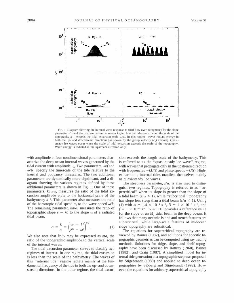
FIG. 1. Diagram showing the internal wave response to tidal flow over bathymetry for the slopeparameter s/a and the tidal excursion parameter ku0/v. Internal tides occur when the scale of thetopography k21 exceeds the tidal excursion scale u0/v. In this regime, waves radiate energy inboth the up- and downstream directions [as shown by the group velocity (cg) vectors]. Quasi-steady lee waves occur when the scale of tidal excursion exceeds the scale of the topography.Wave energy is radiated in the upstream direction only.

with amplitude a, four nondimensional parameters char-acterize the deep-ocean internal waves generated by thetidal current with amplitude u0. Two parameters, v/f andv/N, specify the timescale of the tide relative to theinertial and buoyancy timescales. The two additionalparameters are dynamically more significant, and a di-agram showing the various regimes defined by theseadditional parameters is shown in Fig. 1. One of theseparameters, ku0/v, measures the ratio of the tidal ex-cursion amplitude u0/v to the horizontal scale of thebathymetry k21. This parameter also measures the ratioof the barotropic tidal speed u0 to the wave speed v/k.The remaining parameter, ka/a, measures the ratio oftopographic slope s 5 ka to the slope a of a radiatedtidal beam,

1/22 2k v 2 fa 5 5 . (1)

2 21 2m N 2 v

We also note that ka/a may be expressed as ma, theratio of the topographic amplitude to the vertical scaleof the internal waves.

The tidal excursion parameter serves to classify tworegimes of interest. In one regime, the tidal excursionis less than the scale of the bathymetry. The waves ofthis ‘‘internal tide’’ regime radiate mainly at the fun-damental frequency of the tide in both the up- and down-stream directions. In the other regime, the tidal excur-

sion exceeds the length scale of the bathymetry. Thisis referred to as the ‘‘quasi-steady lee wave’’ regime,with waves that propagate only in the upstream directionwith frequencies 2kU(t) and phase speeds 2U(t). High-er harmonic internal tides manifest themselves mainlyas quasi-steady lee waves.

The steepness parameter, s/a, is also used to distin-guish two regimes. Topography is referred to as ‘‘su-percritical’’ when its slope is greater than the slope ofa tidal beam (s/a . 1), while ‘‘subcritical’’ topographyhas slope less steep than a tidal beam (s/a , 1). Using(1) with v 5 1.4 3 1024 s21, N 5 1 3 1023 s21, andf 5 1 3 1024 s21, a . 0.10 provides a reference valuefor the slope of an M2 tidal beam in the deep ocean. Itfollows that many oceanic island and trench features aresupercritical, while large-scale features of midoceanridge topography are subcritical.

The equations for supercritical topography are re-viewed by Baines (1982), and solutions for specific to-pographic geometries can be computed using ray tracingmethods. Solutions for ridge, slope, and shelf topog-raphy have been discussed by Rattray (1960), Baines(1982), and Craig (1987). A simplified model for in-ternal tide generation at a topographic step was proposedby Stigebrandt (1980) and applied to deep ocean to-pographies by Sjoberg and Stigebrandt (1992). How-ever, the equations for arbitrary supercritical topography

OCTOBER 2002 2885S T . L A U R E N T A N D G A R R E T T

h(x) are difficult to solve due to the necessity of a non-linear bottom boundary condition, w(h) 5 U·=h 1u·=h, where U is the barotropic current vector and (u,w) are the lateral and vertical components of the bar-oclinic velocity. The baroclinic wave response to bar-otropic tidal flow over arbitrary steep topography hasinstead been studied using numerical simulations. Inparticular, numerical studies have been carried out forinternal tides at the Hawaiian Ridge (Holloway and Mer-rifield 1999; Merrifield et al. 2001) and the AleutianRidge (Cummins et al. 2001). Simulations of internaltide generation at steep idealized topographies are pre-sented by Li (2002, manuscript submitted to J. Mar.Res.) and Khatiwala (2002, manuscript submitted toDeep-Sea Res.) The properties of quasi-steady lee waveshave also been studied numerically for atmospheric(Lott and Teitelbaum 1993) and oceanographic (Naka-mura et al. 2000) cases.

Models for internal tide generation by subcritical to-pography have been developed by Cox and Sandstrom(1962), Baines (1973), Bell (1975a,b), Hibiya (1986),and Llewellyn Smith and Young (2002). These modelsapply a linearized bottom boundary condition w(2H)5 U·=h. Two approximations are made in this linear-ization: (i) the neglect of the term u·=h involving thelateral current vector u of the internal tide and (ii) theuse of a constant depth z 5 2H in place of z 5 h(x)in applying the boundary condition. Both of these ap-proximations are justified when the slope parameter sat-isfies s/a K 1. With application of the linear boundarycondition, solutions for arbitrary bathymetry can be ob-tained by superposition.

Bell (1975a,b) considered internal waves generatedat subcritical topography in an ocean of infinite depth.His theory is applicable in both the internal tide andquasi-steady lee wave regimes. The vertical energy fluxEf is a quantity of primary interest for studies of mixing.This quantity is often expressed as a work quantity Ef

5 ^pw& for the wave pressure p, or as the product Ef 5cgEd between the vertical group speed cg and the waveenergy Ed. Bell’s expression for the phase-averaged en-ergy flux produced along bathymetry with a (one sided)power spectrum f(k) is

nN

2 2 2 2 2 2 1/2E 5 2r nv[(N 2 n v )(n v 2 f )]Of 0 bn51

` ku021 23 k J f(k) dk, (2)E n1 2v0

where Nb is the buoyancy frequency along the bottomand Jn is the Bessel function. The index n correspondsto tidal harmonics, with the maximum harmonic nN be-ing the largest integer less than Nb/v. In (2), the powerspectrum is normalized to satisfy f(k) dk 5 , where` 2# h0

is the mean square height of the topography.2hIt is useful to examine the approximate limiting forms

of the Bessel function in (2), which are Jn . [(ku0)/

(2v)]n/n! for ku0 /v K 1, and Jn . cos(ku0 /Ï(2v/pku )0

v 2 np/2 2 p/4) for ku0 /v k 1. In the later expression,the cosine term represents the constructive and destruc-tive interference between quasi-steady lee waves gen-erated during successive tidal periods. The approximatewavenumber dependence of the energy flux for the in-ternal tide of fundamental frequency (n 5 1) is kf(k)for ku0 /v , 1, and k22f(k) for ku0 /v . 1. Thus, thespectrum of energy flux is more ‘‘blue’’ than the bathy-metric spectrum in the internal-tide regime and more‘‘red’’ in the quasi-steady lee wave regime. For the com-mon case of small tidal excursion, the energy flux iswell approximated by

`2 2 2 2 1/21 [(N 2 v )(v 2 f )]b 2E 5 r ku f(k) dk. (3)f 0 E 02 v 0

a. Equivalent modes and finite depth

The integration in (2) is performed over a continuousspectrum of wavenumbers. In Bell’s theory, the internalwaves radiated away from topography are assumed tonever reach the upper ocean, where the waves wouldreflect at the upper surface. This assumption is justifiedif the internal waves are dissipated rapidly after gen-eration. For waves that are not rapidly dissipated, theneglect of upper-ocean reflection is justified only in anocean of infinite depth.

In finite depth formulations, the internal tide responseis modeled as baroclinic modes. The modal dispersionrelation given by

1/22 2jp v 2 fk 5 , (4)2j 1 22H N 2 v

where j 5 1, 2, 3, . . .; dk 5 (p/H) [(v 2 2 f 2)/(2

2Nv 2)]1/2 is the spacing between modes, and H is the depth.Hibiya (1986) derived (4) for the case of constant Nwith f 5 0. Llewellyn Smith and Young (2002) showthat (4) is a valid approximation for the case of a depth-varying stratification when is taken as the depth-av-Neraged stratification, 5 (1/H) N(z) dz. In the finite0N #2H

depth derivations, the integral over continuous wave-numbers in (2) is replaced by a summation over discretemodes, though this sum tends to (2) as the ocean depthtends to infinity.

The primary influence of finite depth on the internaltide energy flux is that the largest scale of internal waveresponse is limited to that of the mode-1 wave. Thissuggests that using k0 5 k1 2 ½dk as the lower limitof integration in (2) provides the first-order finite depthcorrection to Bell’s theory. The magnitude of this cor-rection to the energy flux estimate depends on the shapeof the bathymetric spectrum f(k), with the correctionbeing largest for spectra that are red at low wavenum-bers. There is additional inaccuracy in (2) that ariseswhen doing a continuous integration over wavenumbersinstead of a discrete sum over modes. In practice, this

2886 VOLUME 32J O U R N A L O F P H Y S I C A L O C E A N O G R A P H Y

amounts to only a small error in the integrated estimateof energy flux.

In the calculations that follow, we will integrate (2)from k0 to ` and refer to the wavenumbers given by (4)as ‘‘equivalent modes.’’ This term signifies that the in-ternal-tide response at a given wavenumber kj may neveroccur as an actual baroclinic mode. This is particularlytrue for the internal tides generated at high wavenum-bers, which may dissipate before ever reaching the upperocean. However, by referring to equivalent modes, wemay easily refer to a given wavenumber portion of theinternal-tide spectrum.

b. Energy flux estimates for midocean ridgetopography

1) TOPOGRAPHY IN ONE DIMENSION

Here, we consider internal tides generated at mid-ocean ridge topography. We anticipate that the dominantwavelengths of midocean ridge topography will havesubcritical slopes, justifying the use of subcritical the-ory. We will use Bell’s (1975a,b) theory to estimate theenergy flux according to (2), using k0 5 k1 2 ½dk asthe lower limit of integration.

It has long been established that the roughness ofmidocean ridge topography varies according to thespreading rates of the seafloor (Small and Sandwell1992). In general, the roughness and steepness of ridgetopography are inversely proportional to the spreadingrate of the seafloor. To examine the likely range of en-ergy flux production at midocean ridges, we considertopography from two regions. An example of fast-spreading seafloor topography is taken from a region ofthe East Pacific Rise (EPR) near (178S, 1158W), justsouth of the Garrett Fracture Zone. An example of slow-spreading seafloor topography is taken from a region ofthe Mid-Atlantic Ridge (MAR) near (278S, 148W), justnorth of the Rio Grande Fracture Zone. These two re-gions are useful, as they represent extreme cases. Mul-tibeam bathymetry data for these regions are availablefrom the RIDGE Multibeam Synthesis Project, andmaps showing the data are presented in Fig. 2. Sectionsof multibeam data have 200-m resolution in the lateraldirections.

Bathymetric spectra from these regions were com-puted along several sections of the multibeam data (Fig.3). The spectra have been normalized such that the in-tegrated spectrum gives the mean square height of to-pography, f(k) dk 5 . For each region, spectra` 2# h0

were computed both across the direction of fracturezones (XFZ) and along the direction of fracture zones(FZ). At large horizontal wavelengths (2pk21 . 10 km),the crest and canyon bathymetry of the fracture zonesare the dominant topography. This is evident in the spec-tra, as the XFZ spectra dominate over the FZ spectra atlarge wavelengths. At smaller wavelengths (2pk21 ,10 km) abyssal hills are the dominant mode of topog-

raphy (Goff 1991). These occur primarily in the FZdirection, and their signal is evident in the FZ spectrumfrom the MAR (Fig. 3b). In both EPR and MAR cases,the XFZ spectra contain roughly twice the variance ofthe FZ spectra.

Slope spectra follow directly from the bathymetricspectra as k2f(k), and the slope spectra for the acrossFZ bathymetry are also shown in Fig. 3. The meansquare slope ( ) at any wavenumber k can be calculated2sby integrating the slope spectrum,

k

2 2s(k) 5 k9 f(k9) dk9. (5)EIn general, there will exist some wavenumber kc wheres(kc) 5 a, the slope corresponding to critical generationof a tidal beam. The topographic slopes on wavelengthsgreater than 2p are subcritical, while the topographic21kc

slopes on wavelengths less than 2p are supercritical.21kc

The possible range of critical slope wavenumbers forthe EPR and MAR data is shown in Fig. 3. These wave-numbers correspond to topography with horizontalwavelengths of roughly 1 km.

The length scale corresponding to the amplitude ofthe tidal excursion u0/v is an additional important pa-rameter, requiring estimates of the tidal velocities. Bar-otropic tidal velocity data for the EPR and MAR sitesconsidered here were produced using the TPXO.3 globaltidal model (Egbert et al. 1994; Egbert 1997) for theyear between 1 January 2000 and 1 January 2001. Re-cords of barotropic tidal currents (U, V) were producedat 28 Mercator intervals spanning the bathymetric sec-tions. The M2 components of these records were ex-tracted, and tidal ellipses were computed using standardmethods (e.g., Godin 1972). The spatially averaged M2

tidal ellipses for each site are shown in Fig. 4. Currentamplitudes along the semimajor and semiminor axes ofthe ellipses were projected onto the FZ and XFZ direc-tions to give estimates of u0 for use in the energy fluxcalculations. Current amplitudes along the EPR bathym-etry are (0.010, 0.008) m s21 for the (FZ, XFZ) direc-tions, respectively. The corresponding current ampli-tudes for the MAR bathymetry are (0.031, 0.026) m s21.Tidal excursion amplitudes in the XFZ directions are53 m and 185 m for the EPR and MAR sites, respec-tively.

Topographic slopes on wavelengths greater than 1 kmare subcritical. Therefore, we assume that theory forsubcritical topography is applicable, and we use thespectra of XFZ bathymetry shown in Fig. 3 with ex-pression (2) to calculate energy flux spectra. The finespatial resolution of these one-dimensional sections al-low us to examine the spectrum of energy flux to verylarge equivalent modes.

For these calculations, stratification data providesboth the bottom value of buoyancy frequency in (2),and also the buoyancy scaling for the modal dispersionrelation (4). Buoyancy frequency profiles for the EPR

OCTOBER 2002 2887S T . L A U R E N T A N D G A R R E T T

FIG. 2. Multibeam bathymetry data from the (a) EPR and (b) MAR. Bathymetric sections weretaken along fracture zones (FZ) and across fracture zones (XFZ) to calculate spectra. Boxed regionsindicate the locations of several sections described in the text.

2888 VOLUME 32J O U R N A L O F P H Y S I C A L O C E A N O G R A P H Y

FIG. 3. Bathymetric spectra for the (a) EPR and (b) MAR from sections shown in Fig. 2. The standard deviations ofthe spectral estimates are represented by the shaded bands. In each panel, the slope spectra of the XFZ bathymetry arealso shown. The wavenumber of the tidal excursion scale v/u0 is shown for each site. The range of wavenumbersassociated with subcritical and critical slopes for each XFZ spectrum is indicated.

and MAR regions are shown in Fig. 5. These profileswere derived from temperature and salinity data fromthe Levitus et al. (1994) and Levitus and Boyer (1994)database, and approximate fits to each profile are shownin the figure. An exponential profile N 5 N0 exp(z/b)with N0 5 0.005 24 s21 and b 5 1300 m was used forthe stratification at the EPR site. An offset of N1 50.0005 s21 was added to the exponential dependence toaccount for the contrast between North Atlantic DeepWater and Antarctic Bottom Water below 3000 m at theMAR site. While these simple fits have rather poor fi-delity at any given depth, they do capture the generalstructure of the stratification, and thus provide the basisfor an estimate of for use in (4). For the exponentialNfit with the offset, the equivalent mode dispersion re-lation can be approximated as

2 2 1/2jp(v 2 f )k 5 , (6)j N b 1 N H0 1

where the denominator was taken as (2

2 v2)1/2H øNH since

2k v2. In the case of an exponential strat-N N

ification with no offset (EPR case), the dispersion re-lation (6) has no dependence on the depth H.

Energy flux estimates were made using frequency pa-rameters v 5 1.4 3 1024 s21 for the M2 tide, f 5 (24.33 1025, 27.3 3 1025) s21, and Nb 5 (6 3 1024, 1 31023) s21, for the EPR and MAR sites respectively.These bottom values of buoyancy frequency were takenfrom the data in Fig. 5, not from the exponential fits tothe profiles. Tidal current amplitudes of 0.008 m s21

(EPR) and 0.026 m s21 (MAR) were used to calculate

the XFZ spectra, which are shown in Fig. 6. Estimatedequivalent mode numbers from (6) are given along theupper axes. Spectra from both EPR and MAR sites are‘‘blue’’ with a dependence that is roughly k3/2 at lowwavenumbers and ‘‘red’’ with a dependence that isroughly k22–k23 for the high wavenumbers. The spectralpeaks occur near mode 8 in the EPR data, and nearmode 5 in the MAR data.

The integrated energy flux of these XFZ spectra areroughly 0.2 and 4.3 mW m22 for the EPR and MARsites respectively. Integrated energy flux levels for theFZ sections were roughly 0.1 mW m22 (EPR) and 5.7mW m22 (MAR). Bathymetric variance levels for dif-ferent sections at a given site exhibit 50% variations,even between adjacent sections. Also, the relative ori-entation of the tidal ellipse to a given section influencesthe energy flux estimate significantly because of thedependence of (2) on . However, estimates of total2u0

energy flux are rather insensitive to the lower and upperlimits of integration, as the dominant contributions tothe integrals come from the bandwidths around the spec-tral peaks. Figure 6 shows the cumulative integratedpower along the full spectrum of wavenumbers. In bothEPR and MAR cases, over two-thirds of the total poweroccurs in equivalent modes 1–10. Equivalent modes 1–30 contain over 80% of the total power.

The MAR site clearly produces stronger internal tidesthan the EPR site. This is due to both the MAR’s in-creased topographic roughness and stronger barotropictides. Some additional details of the internal-tide esti-mates for the MAR site are listed in Table 1. Estimates

OCTOBER 2002 2889S T . L A U R E N T A N D G A R R E T T

FIG. 4. Tidal ellipses of the barotropic M2 currents at the (a) EPR and (b) MAR sites. In both cases, thecurrent vectors turn in the clockwise direction over the M2 tidal period. The axes defined by the semimajorand semiminor currents (Ue, Ve), and the axes aligned with FZ and XFZ directions are also shown.

FIG. 5. Profiles of buoyancy frequency N from the (a) EPR and (b) MAR sites. Approximateexponential fits to the data are shown.

of root-mean-square (rms) current speeds for variousspectral bandwidths were calculated according to Bell’stheory,

1/2k922v k9u02u 5 J f(k9) dk9 . (7)E 12 1 2[ ]a v

For example, the rms current associated with equivalentmode 1 was calculated by integrating (7) over the band-width k1 , k , (3/2)k1. The estimates in Table 1 show1

2

that for equivalent modes greater than 30, the rms cur-rent of the internal tide is comparable to the barotropiccurrent. This demonstrates that the applicability of sub-critical theory breaks down at high equivalent modes.

2) TOPOGRAPHY IN TWO DIMENSIONS

Here, we consider the energy flux calculation for to-pography that varies in both lateral directions. In gen-eral, the components of a tidal current can be expressedas (U, V) 5 [u0 cos(vt), y0 cos(vt 1 q)], where q isthe relative temporal phase between U and V. LlewellynSmith and Young (2002) have considered this generalcase. However, for a given tidal ellipse, the semimajorand semiminor current components can be expressed as(Ue, Ve) 5 [ue cos(vt), ye sin(vt)]. All phase informationis absorbed into the tidal ellipse parameters such thatthe semimajor and semiminor components are exactlyout of phase (Godin 1972). In this reference frame, sub-

2890 VOLUME 32J O U R N A L O F P H Y S I C A L O C E A N O G R A P H Y

FIG. 6. Energy flux spectra from the (a) EPR and (b) MAR sites. Standard deviations of the spectral estimates areindicated by the shaded bands. For each site, the wavenumber range for critical slopes and the tidal excursion scaleare indicated. The cumulative integrals of energy flux are also shown. The equivalent modes are given along the upperaxes for reference.

TABLE 1. Vertical energy flux and baroclinic currents for the M2

internal tide calculated for a section of XFZ Mid-Atlantic Ridge to-pography. A barotropic current amplitude of 0.026 m s21 was usedin (2) and (7) for these estimates. Values for other parameters aregiven in the text.

Integratedbandwidth

Energy flux Ef

(mW m22)Rms current speed

(m s21)

All modesMode 1Modes 1–5Modes 1–10Modes 1–30

4.25 6 20.221.012.423.55

0.020 6 0.0040.00130.00360.00680.0104

critical theory allows the bottom boundary conditionfor the vertical velocity to be expressed as

]h ]hw(2H ) 5 u cos(vt) 1 y sin(vt) , (8)e e]x ]ye e

where (xe, ye) are the coordinates aligned with the semi-major and semiminor axes. Using standard internal waverelations for wave pressure p, or for the vertical groupspeed cg, and energy density Ed (e.g., Gill 1982, 258–267), the vertical energy flux can be expressed as

2 2 2 2 1/2[(N 2 v )(v 2 f )]b 2E 5 r ^w &, (9)f 0 2 2 1/2v(k 1 l )

where ^·& is an average over all components of wavephase. This expression for energy flux is only valid forthe internal tide response at length scales much largerthan the tidal excursion. The energy flux can be ex-pressed as

2 2 2 2 1/21 [(N 2 v )(v 2 f )]bE 5 rf 02 v

2p `

2 2 2 2 23 (u cos u 1 y sin u)K f(K, u) dK du.E E e e

0 K1

(10)

Here (k, l) are the wavenumbers corresponding to the(xe, ye) coordinates, K 5 (k2 1 l2)1/2 is the total wave-number, and u 5 tan21(l/k). The power spectrum oftopography is normalized to satisfy f(K, u)K dK`2p# #0 0

du 5 .2hTo evaluate (10), a two-dimensional power spectrum

must be defined from bathymetry. The multibeam datapreviously discussed are inadequate for this purpose be-cause of their nonuniform coverage. Gridded bathym-etry data from satellite altimetry and ship sounding re-cords have been prepared by Smith and Sandwell (1997,version 8.2; SS97 hereafter). These data provide fullspatial coverage, though at a coarse resolution of rough-ly 3 km. However, given the red spectrum of internaltide energy flux, the SS97 data are adequate for resolv-ing the spatial scales accounting for most of the energy.

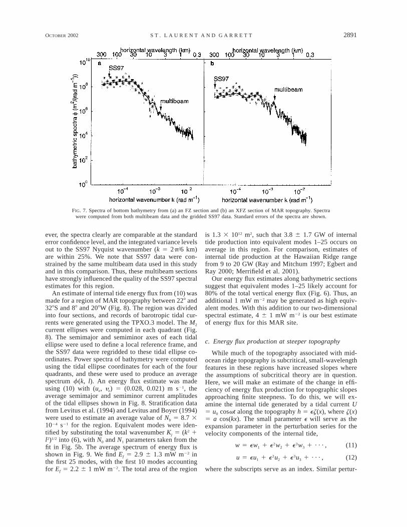
As a means of assessing the quality of spectra com-puted from the SS97 data for the MAR site (Fig. 2b),we have computed spectra along the same bathymetricsections used with the multibeam data. The SS97 spectraare shown along with multibeam spectra in Fig. 7. TheSS97 spectra have been wavenumber averaged with a3-point running boxcar, and standard error confidencebands are shown. The SS97 data are noisier and morestatistically uncertain, as they contain significantly few-er degrees of freedom than the multibeam spectra. How-

OCTOBER 2002 2891S T . L A U R E N T A N D G A R R E T T

FIG. 7. Spectra of bottom bathymetry from (a) an FZ section and (b) an XFZ section of MAR topography. Spectrawere computed from both multibeam data and the gridded SS97 data. Standard errors of the spectra are shown.

ever, the spectra clearly are comparable at the standarderror confidence level, and the integrated variance levelsout to the SS97 Nyquist wavenumber (k 5 2p/6 km)are within 25%. We note that SS97 data were con-strained by the same multibeam data used in this studyand in this comparison. Thus, these multibeam sectionshave strongly influenced the quality of the SS97 spectralestimates for this region.

An estimate of internal tide energy flux from (10) wasmade for a region of MAR topography between 228 and328S and 88 and 208W (Fig. 8). The region was dividedinto four sections, and records of barotropic tidal cur-rents were generated using the TPXO.3 model. The M2

current ellipses were computed in each quadrant (Fig.8). The semimajor and semiminor axes of each tidalellipse were used to define a local reference frame, andthe SS97 data were regridded to these tidal ellipse co-ordinates. Power spectra of bathymetry were computedusing the tidal ellipse coordinates for each of the fourquadrants, and these were used to produce an averagespectrum f(k, l). An energy flux estimate was madeusing (10) with (ue, ye) 5 (0.028, 0.021) m s21, theaverage semimajor and semiminor current amplitudesof the tidal ellipses shown in Fig. 8. Stratification datafrom Levitus et al. (1994) and Levitus and Boyer (1994)were used to estimate an average value of Nb 5 8.7 31024 s21 for the region. Equivalent modes were iden-tified by substituting the total wavenumber Kj 5 (k2 1l2)1/2 into (6), with N0 and N1 parameters taken from thefit in Fig. 5b. The average spectrum of energy flux isshown in Fig. 9. We find Ef 5 2.9 6 1.3 mW m22 inthe first 25 modes, with the first 10 modes accountingfor Ef 5 2.2 6 1 mW m22. The total area of the region

is 1.3 3 1012 m2, such that 3.8 6 1.7 GW of internaltide production into equivalent modes 1–25 occurs onaverage in this region. For comparison, estimates ofinternal tide production at the Hawaiian Ridge rangefrom 9 to 20 GW (Ray and Mitchum 1997; Egbert andRay 2000; Merrifield et al. 2001).

Our energy flux estimates along bathymetric sectionssuggest that equivalent modes 1–25 likely account for80% of the total vertical energy flux (Fig. 6). Thus, anadditional 1 mW m22 may be generated as high equiv-alent modes. With this addition to our two-dimensionalspectral estimate, 4 6 1 mW m22 is our best estimateof energy flux for this MAR site.

c. Energy flux production at steeper topography

While much of the topography associated with mid-ocean ridge topography is subcritical, small-wavelengthfeatures in these regions have increased slopes wherethe assumptions of subcritical theory are in question.Here, we will make an estimate of the change in effi-ciency of energy flux production for topographic slopesapproaching finite steepness. To do this, we will ex-amine the internal tide generated by a tidal current U5 u0 cosvt along the topography h 5 ez(x), where z(x)5 a cos(kx). The small parameter e will serve as theexpansion parameter in the perturbation series for thevelocity components of the internal tide,

2 3w 5 ew 1 e w 1 e w 1 · · · , (11)1 2 3

2 3u 5 eu 1 e u 1 e u 1 · · · , (12)1 2 3

where the subscripts serve as an index. Similar pertur-

2892 VOLUME 32J O U R N A L O F P H Y S I C A L O C E A N O G R A P H Y

FIG. 8. Map showing the region of MAR topography used in calculations of internal tide energy flux.Tidal ellipses of M2 currents are also shown.

bation expansions follow for p and r in the governingequations

]u 1 ]p5 2 , (13)

]t r ]x0

]w 1 ]p g5 2 2 r, (14)

]t r ]z r0 0

]r ]r2 w 5 0, (15)

]t ]z

]u ]w1 5 0. (16)

]x ]z

We have neglected advective terms that scale with thetemporal rate of change terms as ku0 /v. This is justifiedby the assumption that the tidal excursion scale is muchless than the scale of the topography, thus limiting thisanalysis to the internal-tide-regime solution of the gov-

erning equations. Quasi-steady lee waves will not beconsidered here. We seek the solution of (13)–(16) sub-ject to the bottom boundary condition

]hw(h) 5 (U 1 u) . (17)

]x

We begin by considering Taylor series for the com-ponents of the internal tide velocity:

2]w 1 ] w2w(h) 5 w(2H ) 1 h 1 h 1 · · · , (18)

2]z 2 ]z2]u 1 ] u

2u(h) 5 u(2H ) 1 h 1 h 1 · · · , (19)2]z 2 ]z

where all terms are evaluated at z 5 2H, the meandepth of the topography. The bottom boundary condi-tion (17) together with (11), (12), (18), and (19) allowsus to write

OCTOBER 2002 2893S T . L A U R E N T A N D G A R R E T T

FIG. 9. Two-dimensional spectrum of energy flux in a four-quadrant wavenumber space. Thewavenumber axes were taken along the semimajor (k) and semiminor (l) axes of the tidal ellipsereference frame. Circles correspond to the equivalent modes 1, 10, and 25.

]zw 5 U , (20)1 ]x

]z ]w1w 5 u 2 z , (21)2 1 ]x ]z2]z ]u ]z ]w 1 ] w1 2 12w 5 u 1 z 2 z 2 z , (22)3 2 2]x ]z ]x ]z 2 ]z

and so on for higher-order terms. The first-order solutionsatisfies the linearized form of the bottom boundarycondition,

w 5 2aku sinkx cos(mz 1 vt),1 0 (23)

where m 5 kN/v is the vertical wavenumber of the ra-diated internal tide. Higher-order corrections follow as

2w 5 2a kmu sin2kz sin(2mz 1 vt), (24)2 0

13 2w 5 a km u [sinkx cos(mz 1 vt)3 08

1 9 sin3kx cos(3mz 1 vt)]. (25)

The vertical energy flux is

2 4E 5 e ^p w & 1 e ^p w 1 p w 1 p w & 1 · · ·f 1 1 2 2 1 3 3 1

65 E 1 E 1 O(e ), (26)f f1 2

where the ^·& operation is an average over all compo-nents of the wave phase. Here, we have defined theE terms such that each includes a factor e2n. Extendingfn

the series in (26) to additional higher-order correctionsbecomes algebraically tedious, as each successive nthcorrection requires correction of p and w to order (2n2 1). However, the first two terms for the energy flux

2894 VOLUME 32J O U R N A L O F P H Y S I C A L O C E A N O G R A P H Y

follow easily from (23)–(25) along with the correspond-ing terms in the perturbation series for p,

12 2 2E 5 r kNu e a , (27)f 0 01 4

12 2 4 4E 5 r kNu m e a . (28)f 0 02 16

Rewriting (28) using the relation for the aspect ratio ofthe internal tide beam, a 5 k/m, we have

21 sE 5 E , (29)f f2 11 24 a

where s 5 eka is the slope of the topography. The pa-rameter s/a is the slope parameter discussed in section 2.

We have presented the perturbation expansion of en-ergy flux (26) as a means of assessing the change inefficiency of power production as topographic slopes ofincreasing steepness are considered. Higher-order cor-rections are clearly necessary to accurately assess thetrue change in energy flux for topography with finitesteepness. However, we find the first correction is arather small adjustment to the linear solution. We there-fore suggest that the energy flux prediction of subcriticaltheory provides a useful estimate of internal tide powerfor general topographic slopes with s , a. This con-clusion is supported by the work of Balmforth et al.(2002), who have extended the series in (26) using MA-PLE. They find a convergent series for the case of si-nusoidal topography with maximum steepness satisfy-ing the critical condition s/a 5 1, predicting a 56%increase in the energy flux production over the linearsolution. Balmforth et al. also consider the case of aGaussian seamount, finding only a 14% increase in en-ergy flux over the linear prediction. The numerical re-sults of Li (2002, manuscript submitted to J. Mar. Res.)indicate a 70% increase over the linear prediction ofenergy flux for critical sinusoidal topography. For su-percritical slopes, Li finds that a reduction in the buoy-ancy stratification inhibits the generation of internaltides, with a significant decrease in energy flux, thoughthis result is sensitive to the model’s dissipation scheme.Khatiwala (2002, manuscript submitted to Deep-SeaRes.) also finds reduced energy-flux production at su-percritical topography. Further research on supercriticalgeneration is needed.

3. Discussion

a. Shear instability

Once generated, a beam of internal-tide energy willradiate off the bottom and away from the generationsite. The radiated internal tide will be stable to shear(uz) if the Richardson number (Ri 5 N2/ ) is greater2uz

than unity at all depths. The shear stability of the ra-diated internal tide (in isolation from other currents withshear) can be computed for the case of subcritical to-

pography by integrating a function of the bathymetricspectrum f(k). An expression for the Richardson num-ber’s dependence on vertical wavenumber (m) followsfrom (7),

21m922v amu02 2 2Ri(m9) 5 N m J f(am) dm , (30)E 11 2[ ]a v

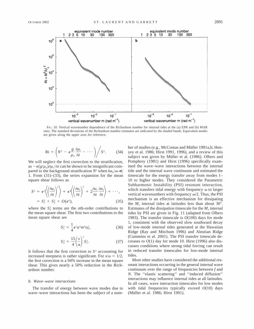
where the expression in brackets is an integral over thespectrum of shear for the internal tide of fundamentalfrequency. Figure 10 shows the Richardson numbercomputed using (30) with the XFZ bathymetry spectrashown in Fig. 3. For the case of internal tides abovethe EPR, the estimated Richardson number exceeds uni-ty at all vertical wavelengths larger than O(10) m. In-ternal tides above the MAR site have larger shear, withRi . 1 at a vertical scale of m21 . 10 m, or an equivalentmode of 300. For these high modes, the influence ofcritical topography during internal-tide generation islikely significant, and our estimates of Ri at high modesare rather questionable. However, we have estimatedthat such high-mode waves carry a negligible amountof the internal-tide energy flux. Thus, very little internaltide power is likely to dissipate by shear instability im-mediately after generation from midocean ridge topog-raphy.

Observations by Lueck and Mudge (1997) and Lienand Gregg (2001) suggest that higher levels of shearand turbulence occur at sites of internal-tide generationby supercritical topography. At these sites, observedlevels of dissipation may be the result of shear insta-bility. However, this local dissipation may representonly a small fraction of the radiated internal-tide energy.For example, recent observations at the Mendocino Es-carpment and at Hawaiian Ridge suggest that dissipationnear the topography is about 10% of the energy fluxradiated away as low-mode internal tides (E. Kunze2002, personal communication).

To examine the potential for enhanced internal-tideshear at topographic slopes of finite steepness, we againconsider the perturbation series solution for waves gen-erated by tidal flow over h(x) 5 ea cos(kx) topography.The first three terms in the series for shear are given by

]u1 2e 5 eam u coskx cos(mz 1 vt), (31)0]z

]u22 2 2 3e 5 2e a m u cos2kx sin(2mz 1 vt), (32)0]z

]u 133 3 3 4e 5 2 e a m u [coskx cos(mz 1 vt)0]z 81 27 cos3kx cos(3mz 1 vt)].

(33)

To examine changes in the stability of the internaltide to shear, we must consider corrections to meansquare shear S 2 to calculate the Richardson number

OCTOBER 2002 2895S T . L A U R E N T A N D G A R R E T T

FIG. 10. Vertical wavenumber dependence of the Richardson number for internal tides at the (a) EPR and (b) MARsites. The standard deviations of the Richardson number estimates are indicated by the shaded bands. Equivalent modesare given along the upper axes for reference.

g ]r12 2Ri 5 N 2 e 2 · · · S . (34)1 2@r ]z0

We will neglect the first correction to the stratification,as 2e(g/r 0)]r1/]z can be shown to be insignificant com-pared to the background stratification N2 when ku0 /v K1. From (31)–(33), the series expansion for the meansquare shear follows as

2 2]u ]u ]u ]u1 2 1 32 2 4S 5 e 1 e 1 2 1 · · · ,71 2 8 71 2 8]z ]z ]z ]z

2 2 65 S 1 S 1 O(e ),1 2 (35)

where the terms are the nth-order contributions to2Sn

the mean square shear. The first two contributions to themean square shear are

12 2 2 4 2S 5 e a m u , (36)1 04

215 s2 2S 5 S . (37)2 11 24 a

It follows that the first correction to S 2 accounting forincreased steepness is rather significant. For s/a 5 1/2,the first correction is a 94% increase in the mean squareshear. This gives nearly a 50% reduction in the Rich-ardson number.

b. Wave–wave interactions

The transfer of energy between wave modes due towave–wave interactions has been the subject of a num-

ber of studies (e.g., McComas and Muller 1981a,b; Hen-yey et al. 1986; Hirst 1991, 1996), and a review of thissubject was given by Muller et al. (1986). Olbers andPomphrey (1981) and Hirst (1996) specifically exam-ined the wave–wave interactions between the internaltide and the internal wave continuum and estimated thetimescale for the energy transfer away from modes 1–10 to higher modes. They considered the ParametricSubharmonic Instability (PSI) resonant interaction,which transfers tidal energy with frequency v to largervertical wavenumbers with frequency v/2. Thus, the PSImechanism is an effective mechanism for dissipatingthe M2 internal tides at latitudes less than about 308.Estimates of the dissipation timescale for the M2 internaltides by PSI are given in Fig. 11 (adapted from Olbers1983). The transfer timescale is O(100) days for mode1, consistent with the observed slow southward decayof low-mode internal tides generated at the HawaiianRidge (Ray and Mitchum 1996) and Aleutian Ridge(Cummins et al. 2001). The PSI transfer timescale de-creases to O(1) day for mode 10. Hirst (1996) also dis-cusses conditions where strong tidal forcing can resultin reduced transfer timescales for low-mode internaltides.

Most other studies have considered the additional res-onant interactions occurring in the general internal wavecontinuum over the range of frequencies between f andN. The ‘‘elastic scattering’’ and ‘‘induced diffusion’’interactions may influence internal tides at all latitudes.In all cases, wave interaction timescales for low modeswith tidal frequencies typically exceed O(10) days(Muller et al. 1986; Hirst 1991).

2896 VOLUME 32J O U R N A L O F P H Y S I C A L O C E A N O G R A P H Y

FIG. 11. The timescales for wave–wave (PSI) interactions between the M2 internal tide andthe internal wave continuum for modes 1, 2, 3, 5, and 10, adapted from Olbers (1983). The PSIinteraction for the M2 tide occurs equatorward of 6308 lat. Bottom reflection times for the variousmodes were estimated for an exponential stratification over a depth of 4000 m.

It is useful to compare the wave interaction timescaleto the time for a wave group to travel from bottom tosurface and back again, defined according to

21t 5 2# c dz,g g

where the integral is over the ocean depth and cg is thevertical component of the group speed. The latitude andmode-number-dependent curves for tg were computedusing N 5 N0ez/b with (b, N0) 5 (1300 m, 0.005 24 s21),and the results are shown in Fig. 11. Low modes havethe fastest group speeds, with tg # 12 h for mode 1 andtg $ 4 days for mode 10. Thus, low modes will easilycomplete one round-trip between the bottom and surfacebefore experiencing the effects of wave–wave interac-tions. For modes j $ 10, energy transfer to higher modeswill occur over a timescale comparable to, or faster than,the bottom reflection time. Thus, wave–wave interac-tions may be the dominant mechanism of spectral evo-lution for high-mode components of the internal tide,while bottom reflection is significant for low modes.

c. Bottom reflection and topographic scattering

The interaction of internal waves with bottom ba-thymetry is often discussed in terms of wave reflectionfrom sloping topography and wave scattering fromrough topography. Particular attention has been givento reflection from planar slopes (e.g., Eriksen 1982,1985; Garrett and Gilbert 1988; Thorpe 1987, 1997,1999). Reflection from slopes with nonplanar geome-tries has been considered by Gilbert and Garrett (1989)

and Muller and Liu (2000a,b). Scattering of waves fromrandom rough topography was considered by Muller andXu (1992), and Thorpe (2001) considered scatteringfrom rough topography with an underlying slope. Forthe midocean ridge topography discussed in section 2b,the latter studies are clearly most relevant.

As discussed by Muller and Xu (1992), both reflectionand scattering redistribute energy flux in wavenumberspace. Muller and Xu (1992) find that scattering is moreefficient than reflection at redistributing energy flux tohigher modes, particularly at tidal and near-inertial fre-quencies. However, Muller and Xu (1992) find less than10% of the incoming radiation is redistributed during ascattering event at typical deep-ocean topography. Mostof the incoming radiation undergoes pure reflection asfrom a flat bottom, such that the wavenumber contentof the spectrum is mostly preserved.

Here, we consider the similarity between internal-tidegeneration and the scattering of low-mode internal tides.In this simple calculation, we exploit the fact that thewave response to a mode-1 current flowing over smalltopographic wavelengths is much the same as the waveresponse to a barotropic current. We will examine thescattering of the mode-1 internal tide through a ‘‘secondgeneration’’ calculation, where the amplitude of themode-1 current is used in place of the amplitude of thebarotropic current in (2). This is meant to provide acrude estimate of the energy flux scattered from mode1 into higher modes. The rms current for the mode-1internal tide at the MAR site was found to be u 5 0.0013

OCTOBER 2002 2897S T . L A U R E N T A N D G A R R E T T

FIG. 12. Spectra of incident and scattered mode-1 energy flux fromMAR bathymetry. The wavenumber range associated with criticalslopes is shown.

m s21 (Table 1), corresponding to a current amplitudeof u 5 0.0018 m s21. The incident and scatteredÏ2spectra of energy flux are shown in Fig. 12. The re-sulting estimate of scattered energy flux, integrated overall scattered wavenumbers, is roughly 0.023 mW m22.This compares to an incident mode-1 energy flux ofroughly 0.22 mW m22. Thus, we find mode-1 scatteringoccurs with an efficiency of about 10%, comparable tothe efficiencies estimated by Muller and Xu (1992). Wenote that in our estimate, a small amount of scatteredenergy flux is predicted in the lowest several modes, soour scattering efficiency is a bit high.

4. Conclusions

Having considered the various mechanisms that canact to degrade the internal tides into turbulence, it ispossible to speculate about the nature of internal-tide-driven mixing in the deep ocean. Low-mode waves arerelatively uninfluenced by wave–wave interactions andtheir Richardson numbers are large. In regions whereadditional sheared currents are absent, low modes willpropagate away from their generation sites, carryingmuch of the generated energy flux. The lateral distancefor one round-trip between the bottom and surface canbe estimated using the characteristic equation for a tidalbeam, dx/dz 5 a21, such that

1/20 2 2N (z) 2 vDx 5 2 dz. (38)E 2 2[ ]v 2 f

2H

For typical stratification in the deep ocean, this radiation

distance is Dx . 100 km. Thus, waves correspondingto low modes can be expected to travel O(100 km)before scattering from topography. During topographicscattering, much of the low-mode energy flux is pre-served, suggesting that low modes can radiate throughmany bottom encounters. Observations of internal tidesgenerated at Hawaii (Ray and Mitchum 1996) and theAleutian Ridge (Cummins et al. 2001) demonstrate thatlow modes can be tracked for O(1000) km away fromtheir generation site.

Most internal-tide-driven mixing must be supportedby high equivalent modes that have more shear, makingthem more likely to dissipate locally by shear instability.This is particularly true of internal tides generated atcritical slopes, such as those found along supercriticaltopography. Wave–wave interactions are also more ef-ficient for higher modes, providing another mechanismfor converting internal tide energy flux into turbulence.The ‘‘Parametric Subharmonic Instability’’ interactionis particularly effective since it specifically moves en-ergy to higher equivalent modes. However, the PSImechanism for tidal frequencies is only effective at lowlatitudes. The effectiveness of other classes of wave–wave interactions at transferring wave energy to highermodes is unclear, though some ideas are presented byPolzin (1999).

The wave–wave interaction timescale for equivalentmode 10 is roughly equal to the timescale over whichthe mode-10 tidal beam completes a round-trip betweenthe bottom and surface. Over this characteristic time-scale, the mode-10 tidal beam radiates roughly 100 kmfrom the generation site. Higher equivalent modes willbe increasingly influenced by the wave–wave interac-tions over shorter time- and distance scales. We suggestthat for a given internal-tide-generation event, waveswith equivalent modes less than 10 are likely to radiateaway, with equivalent modes greater than 10 dissipatinglocally. For the MAR topography considered in section2b, this suggests that roughly one-third of the generatedpower, about 1–2 mW m22, may dissipate as turbulenceat this site. At other sites, the amount of energy fluxavailable in equivalent modes greater than 10 will clear-ly depend on the nature of the topography, and the natureof the barotropic tides. As shown in section 2b, theenergy flux production at site along the EPR is only 0.2mW m21.

Low equivalent modes that radiate away will be in-fluenced by topographic scattering. Energy scattered tohigher modes is more likely to dissipate, so topographicscattering provides a mechanism for driving mixingaway from an internal-tide-generation site. However, theefficiency of topographic scattering is low, with roughly10% of low-mode energy flux being transferred to high-er modes. It is possible that while the scattering effi-ciency for general topographies is low, certain topo-graphic sites may favor enhanced scattering. For ex-ample, Gilbert and Garrett (1989) and Muller and Liu(2000b) find convex topographies are more efficient

2898 VOLUME 32J O U R N A L O F P H Y S I C A L O C E A N O G R A P H Y

than linear or concave topographies at scattering energyto high modes. Thus, in addition to the internal tidesgenerated at such sites, convex topographies may befavored sites for the dissipation of incoming internal-tide energy. At such sites, the scattered waves could actas a catalyst for dissipating the locally generated wavessince elevated shear levels in the scattered waves willcontribute to a lower overall Richardson number.

Given the inefficient nature of topographic scatteringat general topographies, it is likely that low-mode in-ternal tides radiate much of their energy through mul-tiple bottom reflections over O(1000 km) distances. Lowmodes must dissipate somewhere, but the nature of low-mode dissipation is particularly unclear. Perhaps lowmodes are preferentially dissipated in regions of en-hanced sheared currents, such as the equatorial under-currents or the Antarctic Circumpolar Current. Perhapslow modes propagate onto the continental shelves wherethey dissipate in shallow waters. Finally, perhaps lowmodes are dissipated throughout in the interior of thedeep ocean under the slow evolution of wave–wave in-teractions. In this scenario, much of the energy in low-mode internal tides would be uniformly dispersedthrough the oceanic interior. The dissipation of this en-ergy would contribute to background levels of turbu-lence everywhere. The fate of low-mode internal tides,however, remains as a primary question.

Acknowledgments. We thank Eric D’Asaro, Eric Kun-ze, and Bill Young for carefully reviewing the manu-script. We also thank Gary Egbert, Ming Li, StefanLlewellyn Smith, Kurt Polzin, and John Toole for help-ful discussions about this work. Multibeam bathymetrydata were obtained from the RIDGE Multibeam Syn-thesis Project. Comments and suggestions from twoanonymous reviewers also improved this presentation.The authors were supported by the U.S. Office of NavalResearch and the Natural Science and Engineering Re-search Council of Canada.

REFERENCES

Baines, P. G., 1973: The generation of internal tides by flat-bumptopography. Deep-Sea Res., 20, 179–205.

——, 1982: On internal tide generation models. Deep-Sea Res., 29,307–338.

Balmforth, N. J., G. R. Ierley, and W. R. Young, 2002: Tidal con-version by subcritical topography. J. Phys. Oceanogr., 32, 2900–2914.

Bell, T. H., 1975a: Lee waves in stratified flows with simple harmonictime dependence. J. Fluid Mech., 67, 705–722.

——, 1975b: Topographically generated internal waves in the openocean. J. Geophys. Res., 80, 320–327.

Cox, C. S., and H. Sandstrom, 1962: Coupling of surface and internalwaves in water of variable depth. J. Oceanogr. Soc. Japan, 20thAnniversary Volume, 499–513.

Craig, P. D., 1987: Solutions for internal tide generation over coastaltopography. J. Mar. Res., 45, 83–105.

Cummins, P. F., J. Y. Cherniawski, and M. G. G. Foreman, 2001:North Pacific internal tides from the Aleutian Ridge: Altimeterobservations and modelling. J. Mar. Res., 59, 167–191.

Egbert, G. D., 1997: Tidal data inversion: Interpolation and inference.Progress in Oceanography, Vol. 40, Pergamon, 81–108.

——, and R. D. Ray, 2000: Significant dissipation of tidal energy inthe deep ocean inferred from satellite altimeter data. Nature,405, 775–778.

——, and ——, 2001: Estimates of M2 tidal energy dissipation fromTOPEX/POSEIDON altimeter data. J. Geophys. Res., 106, 22 475–22 502.

——, A. F. Bennett, and M. G. G. Foreman, 1994: TOPEX/POSEI-DON tides estimated using a global inverse model. J. Geophys.Res., 99, 24 821–24 852.

Eriksen, C., 1982: Observations of internal wave reflection off slopingbottoms. J. Geophys. Res., 87, 525–538.

——, 1985: Implications of ocean bottom reflection for internal wavespectra and mixing. J. Phys. Oceanogr., 15, 1145–1156.

Garrett, C., and D. Gilbert, 1988: Estimates of vertical mixing byinternal waves reflected off sloping topography. Small-Scale Tur-bulence and Mixing in the Ocean. J. C. J. Nihoul and B. M.Janard, Eds., Elsevier Scientific, 405–424.

Gilbert, D., and C. Garrett, 1989: Implications for ocean mixing ofinternal waves scattering off irregular topography. J. Phys.Oceanogr., 19, 1716–1729.

Gill, A. E., 1982: Atmosphere–Ocean Dynamics. Academic Press,662 pp.

Godin, G., 1972: The Analysis of Tides. University of Toronto Press,264 pp.

Goff, J. A., 1991: A global and regional stochastic analysis of near-ridge abyssal hill morphology. J. Geophys. Res., 96, 21 713–21 737.

Hendershott, M. C., 1981: Long waves and ocean tides. Evolution ofPhysical Oceanography, B. A. Warren and C. Wunsch, Eds., TheMIT Press, 292–341.

Henyey, F. S., J. Wright, and S. M. Flatte, 1986: Energy and actionflow through the internal wave field: An eikonal approach. J.Geophys. Res., 91, 8487–8495.

Hibiya, T., 1986: Generation mechanism of internal waves by tidalflow over a sill. J. Geophys. Res., 91, 7696–7708.

Hirst, E., 1991: Internal wave–wave resonance theory: Fundamentalsand limitations. Dynamics of Oceanic Internal Gravity Waves:Proc. ‘Aha Huliko’ a Hawaiian Winter Workshop, P. Muller andD. Henderson, Eds., Honolulu, HI, University of Hawaii at Man-oa, 211–226.

——, 1996: Resonant instability of internal tides. Ph. D. dissertation,University of Washington, 92 pp.

Holloway, P. E., and M. A. Merrifield, 1999: Internal tide generationby seamounts, ridges and islands. J. Geophys. Res., 104, 25 937–25 951.

Kunze, E., and J. M. Toole, 1997: Tidally driven vorticity, diurnalshear, and turbulence atop Fieberling Seamount. J. Phys. Ocean-ogr., 27, 2663–2693.

Ledwell, J. R., E. T. Montgomery, K. L. Polzin, L. C. St. Laurent,R. W. Schmitt, and J. M. Toole, 2000: Mixing over rough to-pography in the Brazil Basin. Nature, 403, 179–182.

Levitus, S., and T. P. Boyer, 1994: Temperature. Vol. 4, World OceanAtlas 1994, NOAA Atlas NESDIS 4, 117 pp.

——, R. Burgett, and T. Boyer, 1994: Salinity. Vol. 3, World OceanAtlas 1994, NOAA Atlas NESDIS 3, 99 pp.

Lien, R.-C., and M. C. Gregg, 2001: Observations of turbulence ina tidal beam and across a coastal ridge. J. Geophys. Res., 106,4575–4592.

Llewellyn Smith, S. G., and W. R. Young, 2002: Conversion of thebarotropic tide. J. Phys. Oceanogr., 32, 1554–1566.

Lott, F., and H. Teitelbaum, 1993: Linear unsteady mountain waves.Tellus, 45, 201–220.

Lueck, R. G., and T. D. Mudge, 1997: Topographically induced mix-ing around a shallow seamount. Science, 276, 1831–1833.

McComas, C. H., and P. Muller, 1981a: The dynamic balance ofinternal waves. J. Phys. Oceanogr., 11, 970–986.

——, and ——, 1981b: Time scales of resonant interactions amongoceanic internal waves. J. Phys. Oceanogr., 11, 139–147.

Merrifield, M. A., P. E. Holloway, and T. M. Shaun Johnston, 2001:

OCTOBER 2002 2899S T . L A U R E N T A N D G A R R E T T

The generation of internal tides at the Hawaiian Ridge. Geophys.Res. Lett., 28, 559–562.

Muller, P., and N. Xu, 1992: Scattering of oceanic internal waves offrandom bottom topography. J. Phys. Oceanogr., 22, 474–488.

——, and X. Liu, 2000a: Scattering of internal waves at finite to-pography in two dimensions. Part I: Theory and case studies. J.Phys. Oceanogr., 30, 532–549.

——, and ——, 2000b: Scattering of internal waves at finite topog-raphy in two dimensions. Part II: Spectral calculations andboundary mixing. J. Phys. Oceanogr., 30, 550–563.

——, G. Holloway, F. Henyey, and N. Pomphrey, 1986: Nonlinearinteractions among internal gravity waves. Rev. Geophys., 24,493–536.

Munk, W., and C. Wunsch, 1998: Abyssal recipes II: Energetics oftidal and wind mixing. Deep-Sea Res., 45, 1977–2010.

Nakamura, T., T. Awaji, T. Hatayama, and K. Akitomo, 2000: Thegeneration of large amplitude unsteady lee waves by subinertialK1 tidal flow: A possible vertical mixing mechanism in the KurilStraits. J. Phys. Oceanogr., 30, 1601–1621.

Olbers, D. J., 1983: Models of the oceanic internal wave field. Rev.Geophys., 21, 1567–1606.

——, and N. Pomphrey, 1981: Disqualifying two candidates for theenergy balance of oceanic internal waves. J. Phys. Oceanogr.,11, 1423–1425.

Polzin, K. L., 1999: A rough recipe for the energy balance of quasi-steady internal lee waves. Dynamics of Oceanic Internal GravityWaves, II: Proc. ‘Aha Huliko’a Hawaiian Winter Workshop, P.Muller and D. Henderson, Eds., Honolulu, HI, University ofHawaii at Manoa, 117–128.

——, J. M. Toole, J. R. Ledwell, and R. W. Schmitt, 1997: Spatialvariability of turbulent mixing in the abyssal ocean. Science,276, 93–96.

Rattray, M., 1960: On the coastal generation of internal tides. Tellus,12, 54–61.

Ray, R., and G. T. Mitchum, 1996: Surface manifestation of internaltides generated near Hawaii. Geophys. Res. Lett., 23, 2101–2104.

——, and ——, 1997: Surface manifestation of internal tides in thedeep ocean: Observations from altimetry and island gauges. Pro-gress in Oceanography, Vol. 40, Pergamon, 135–162.

Seibold, E., and W. H. Berger, 1996: The Sea Floor—An Introductionto Marine Geology. Springer-Verlag, 356 pp.

Sjoberg, B., and A. Stigebrandt, 1992: Computations of the geo-graphical distribution of the energy flux to mixing processes viainternal tides and the associated vertical circulation in the ocean.Deep-Sea Res., 39, 269–291.

Small, C., and D. Sandwell, 1992: An analysis of ridge axis gravityroughness and spreading rate. J. Geophys. Res., 97, 3235–3245.

Smith, W. H. F., and D. T. Sandwell, 1997: Global sea floor topographyfrom satellite altimetry and ship depth soundings. Science, 277,1956–1962.

Stigebrandt, A., 1980: Some aspects of tidal interaction with FjordConstrictions. Estuarine Coastal Mar. Sci., 11, 151–166.

St. Laurent, L. C., J. M. Toole, and R. W. Schmitt, 2001: Buoyancyforcing by turbulence above rough topography in the abyssalBrazil Basin. J. Phys. Oceanogr., 31, 3476–3495.

Thorpe, S. A., 1987: On the reflection of a train of finite amplitudewaves from a uniform slope. J. Fluid Mech., 178, 279–302.

——, 1997: On the interactions of internal waves reflecting fromslopes. J. Phys. Oceanogr., 27, 2072–2078.

——, 1999: Fronts formed by obliquely reflecting internal waves ata sloping boundary. J. Phys. Oceanogr., 29, 29–38.

——, 2001: Internal wave reflection and scatter from sloping roughtopography. J. Phys. Oceanogr., 31, 537–553.

Wunsch, C., 1975: Internal tides in the ocean. Rev. Geophys., 13,167–182.