58


ISSN 1518-3548 CGC 00.038.166/0001-05
Working Paper Series Brasília n. 196 Oct. 2009 p. 1-57

Working Paper Series Edited by Research Department (Depep) – E-mail: [email protected] Editor: Benjamin Miranda Tabak – E-mail: [email protected] Editorial Assistent: Jane Sofia Moita – E-mail: [email protected] Head of Research Department: Carlos Hamilton Vasconcelos Araújo – E-mail: [email protected] The Banco Central do Brasil Working Papers are all evaluated in double blind referee process. Reproduction is permitted only if source is stated as follows: Working Paper n. 196. Authorized by Mário Mesquita, Deputy Governor for Economic Policy. General Control of Publications Banco Central do Brasil
Secre/Surel/Cogiv
SBS – Quadra 3 – Bloco B – Edifício-Sede – 1º andar
Caixa Postal 8.670
70074-900 Brasília – DF – Brazil
Phones: +55 (61) 3414-3710 and 3414-3565
Fax: +55 (61) 3414-3626
E-mail: [email protected]
The views expressed in this work are those of the authors and do not necessarily reflect those of the Banco Central or its members. Although these Working Papers often represent preliminary work, citation of source is required when used or reproduced. As opiniões expressas neste trabalho são exclusivamente do(s) autor(es) e não refletem, necessariamente, a visão do Banco Central do Brasil. Ainda que este artigo represente trabalho preliminar, é requerida a citação da fonte, mesmo quando reproduzido parcialmente. Consumer Complaints and Public Enquiries Center Banco Central do Brasil
Secre/Surel/Diate
SBS – Quadra 3 – Bloco B – Edifício-Sede – 2º subsolo
70074-900 Brasília – DF – Brazil
Fax: +55 (61) 3414-2553
Internet: http//www.bcb.gov.br/?english
The role of macroeconomic variables insovereign risk
Marco S. Matsumura∗ Jose Valentim Vicente†
The Working Papers should not be reported as representing the viewsof the Banco Central do Brasil. The views expressed in the papers arethose of the author(s) and not necessarily reflect those of the BancoCentral do Brasil.
Abstract
We use a dynamic term structure model with default and observa-ble factors to study the interaction between macro variables and theBrazilian sovereign yield curve. We also calculate the default proba-bilities implied from the estimated model and the impact of macroshocks on those probabilities. Our results indicate that the VIX is themost important macro factor affecting short-term bonds and defaultprobabilities, while the American short-term rate is the most impor-tant factor affecting the long-term default probabilities. Regardingthe domestic variables, only the slope of the local yield curve presentssignificant explanatory power for the sovereign rates and default pro-babilities.
JEL classification: C13, E44, G12.
Keywords: Macro-finance, credit risk, affine term structure models,emerging markets.
∗IPEA, Av. Presidente Antonio Carlos 51 17th floor, Rio de Janeiro, Brazil, 55-21-3515-8533. E-mail: [email protected]. Corresponding author.†Central Bank of Brazil, Av. Presidente Vargas 730 7th floor, Rio de Janeiro, Brazil,
55-21-2189-5762. E-mail: [email protected].
3

1 Introduction
Sovereign risk is a subtype of credit risk related to the possibility of a govern-ment failing to honor its payment obligations. It is a fundamental componentof emerging countries’ yield curves. Sovereign risk is also very important foremerging market firms, since the cost of foreign financing typically rises withthe country risk. Accordingly, the following questions are of particular inter-est: What are the factors most affecting the sovereign yield curve? Whichvariables have greatest impact on default probabilities? This study presentsan empirical investigation of these questions by using an affine term structuremodel with macroeconomic variables and default risk1.
There are two main approaches in credit risk modeling: structural andreduced form models2. While the former provides a link between the probabi-lity of default and firms’ fundamental variables, the latter relies on the marketas the only source of information regarding firms’ credit risk structure. Blackand Scholes (1973) and Merton (1974) proposed the initial ideas concerningstructural models based on options theory. Black and Cox (1976) introducedthe basic structural framework in which default occurs the first time the valueof the firm’s assets crosses a given default barrier. More recently, Leland(1994) extended the Black and Cox (1976) model, providing a significantcontribution to the capital structure theory. In his model, the firm’s incentivestructure determines the default barrier endogenously. That is, default isdetermined as the result of an optimal decision policy carried out by equityholders.
All the papers cited above deal with the corporate credit risk case. How-ever, the sovereign credit risk differs markedly from corporate risk3. Forinstance, it is not obvious how to model the incentive structure of a govern-ment and its optimal default decision, or what “assets” could be seized upondefault. Moreover, post-default negotiating rounds regarding the recoveryrate can be very complex and uncertain. Consequently, the use of structuralmodels to assess the default risk of a country is a delicate question. Not
1In this article, the term “macroeconomic (macro) variable” refers to any observablefactor.
2Giesecke (2004) provides a short introductory survey of credit risk models.3As discussed by Duffie et al. (2003), the main differences are: (i) a sovereign debt
investor may not have recourse to a bankruptcy code at the default event. (ii) sovereigndefault can be a political decision. (iii) the same bond can be renegotiated many times.(iv) it may be difficult to collateralize debt with assets into the country. (v) the governmentcan opt for defaulting on internal or external debt. (vi) in the case of sovereign risk, itis necessary to take into account the role played by key variables such as exchange rates,fiscal dynamics, reserves in strong currency, level of exports and imports, gross domesticproduct, and inflation.
4

surprisingly, it is difficult to find studies of sovereign debt pricing based onthe structural approach4. Therefore, we opt to use reduced models, wherethe default time is a totally inaccessible stopping time that is triggered bythe first jump of a given exogenous intensity process5. This means that thedefault always comes as a “sudden surprise”, which provides more realism tothe model. In contrast, within the class of structural models, the evolutionof assets usually follows a Brownian diffusion, in which there are no suchsurprises and the default time is a predictable stopping time.
Lando (1998), and Duffie and Singleton (1999) develop versions of re-duced models in which the default risk appears as an additional instanta-neous spread in the pricing equation. The spread can be modeled using statefactors. In particular, it can be incorporated into the affine framework ofDuffie and Kan (1996), a widely used model offering a good compromisebetween flexibility and numerical tractability6. Duffie et al. (2003) extendthe reduced model to include the possibility of multiple defaults (or multi-ple “credit events”, such as restructuring, renegotiation or regime switches).The model is estimated in two steps. First, the risk-free reference curveis estimated. Next, the defaultable sovereign curve is obtained conditionalon the first stage estimates. As an illustration, they apply their model toanalyze the term structure of credit spreads for bonds issued by the Rus-sian Ministry of Finance (MinFin) over a sample period encompassing thedefault on domestic Russian GKO bonds in August 1998. They investigatethe determinants of the spreads, the degree of integration between differentRussian bonds and the correlation between the spreads macroeconomic vari-ables. Another paper applying reduced model to emerging markets is Panand Singleton (2008), who analyze the sovereign term structures of Mexico,Turkey, and Korea through a dynamic approach.
Nevertheless, Duffie et al. (2003), and Pan and Singleton (2008) use apure latent variables model. Thereby, the impact of macro factors changeson bond yields can be evaluated only indirectly through, for instance, aregression between observable and unobservable variables. Moreover, in purelatent models, the unobservable factors are abstractions that can, at best, beinterpreted as geometric factors summarizing the yield curve movements, asshown by Litterman and Scheinkman (1991).
The modern literature linking the dynamics of the term structure withmacro factors starts with Ang and Piazzesi (2003), who propose an ingenious
4Exceptions are Xu and Ghezzi (2002) and Moreira and Rocha (2004).5A stopping time is totally inaccessible if it can never be announced by an increasing
sequence of predictable stopping times (see Schonbucher, 2003).6An affine model is a multifactor dynamic term structure model, such that the state
process X is an affine diffusion, and the short short-term rate is also affine in X
5

solution to incorporate observable factors in the original framework of affinemodels. In their model, the macroeconomic factors affect the entire yieldcurve. However, the interest rates do not affect the macroeconomic factors,which means that monetary policy is ineffective. Similarly to Duffie et al.(2003), they employ a two-step estimation procedure, first determining themacro dynamics and then the latent dynamics conditional on the macrofactors. Ang et al. (2007) estimate a dynamic macro-finance model usingMarkov Chain Monte Carlo (MCMC) technique in a single step procedure.Others studies that combine macro factors and no-arbitrage conditions areRudebusch and Wu (2004) and Hordal et al. (2008).
Following the advances brought by these previous studies, we examinethe impact of macro factors on a defaultable term structure through an affinemodel similar to that of Ang and Piazzesi (2003). We provide a comparisonamong a variety of specifications in order to determine the macro factors thatmost affect credit spreads and default probabilities of an emerging country.We also use impulse response and variance decomposition techniques to an-alyze the direct influence of observable macro factors on yields and defaultprobabilities.
However, before estimating the parameters, one must choose an identi-fication strategy. Not all parameters of the multifactor affine model can beestimated, since there are transformations of the parameter space preservingthe likelihood. When sub-identified, parameters can be arbitrarily rotated,while over-identified specifications may distort the true response of the statevariables. Based on the findings of Dai and Singleton (2000), we propose anidentification procedure for affine models with macro factors and default7.
We select Brazil as the case study. The reason for this choice is thatBrazil is one of the most important emerging countries with a rich historyof credit events8. When using Brazilian data, one must take into accountthat frequent regime switches have occurred until recently, such as changefrom very high inflation to a stable economy (July 1994), change from fixedto floating exchange rate in a currency crisis in January 1999, and changeof monetary policy to inflation targeting in July 1999. Thus, our samplecomprises five and a half years of historical series. This sample size is com-patible with that found in other recent academic studies containing datafrom emerging economies (see, for instance, Pan and Singleton, 2008, andAlmeida and Vicente, 2009). Furthermore, following these authors, we de-
7Related to our specification analysis there is the work of Pericoli and Taboga (2008),who implement an identification of a default-free affine model with macro factors.
8Jointly with India, Russia and China, Brazil is considered as among the fastest growingdeveloping economies in the world. Goldman Sachs refers to these countries as BRICs, anacronym for Brazil, Russia, India and China (see Goldman Sachs, 2007).
6
cided to employ continuous-time modeling with high-frequency data in orderto avoid small-sample biases.
Our main model contains five state variables: one latent factor for thereference default-free curve, one external macro factor, one internal macrofactor, and two latent factors for the Brazilian sovereign yield curve. We testthe following observable variables: Fed interest rates, VIX (index of impliedvolatility of options in the Standard & Poor’s index), Brazilian Real/US Dol-lar exchange rates, Sao Paulo Stock Exchange index (Ibovespa), and Brazilianinterest rate swaps. In the estimation stage we follow common practice anduse a two-step procedure as implemented by Duffie et al. (2003).
In a nutshell, we contribute to the finance literature in at least two as-pects. First, we extend the works of Duffie et al. (2003) and Pan and Sin-gleton (2008) by incorporating macro variables in a dynamic term structuremodel with default risk. Second, our model allows a full interaction betweenlatent and observable sovereign factors, which in a sense extends the studyof Ang and Piazzesi (2003)9.
Our main findings can be summarized as follows. First, VIX and Fedrates strongly affect the default probabilities in the short and in the longterm, respectively. Second, VIX has a great effect on Brazilian sovereignyields, more than any investigated domestic macro indicator. This resultagrees with one of Pan and Singleton’s (2008) conclusions who report thatVIX has the most explanatory power for Mexican credit default swap (CDS)spreads. Third, among the observable domestic factors only the slope ofyield curve presents significant explanatory power of the Brazilian credit riskspread. Finally, a latent factor highly correlated with the level of the Brazil-ian sovereign curve predicts a substantial fraction of the yield and defaultprobability movements. We also assert that the Brazilian spread is more sen-sitive to volatility of international markets (measured in our model by VIX)than local conditions. On the other hand, the moderate significance of thedomestic yield curve slope indicates that expectations of Brazilian investorsplay a role in determining the sovereign yield and default probabilities.
The rest of this article is organized as follows. In Section 2 we present themodel. Section 3 describes the dataset used. Section 4 details the estima-tion procedure. Section 5 presents the results of implementing the dynamicmodels. Section 6 offers concluding remarks. Auxiliary results are containedin the Appendices.
9Diebold et al. (2006), using a statistical model, find strong evidence of two-wayinteraction between latent and macro factors.
7
2 Affine Model with Default Risk and Macro
Factors
Uncertainty in the economy is characterized by a filtered probability space(Ω, (Ft)t≥0 ,F ,P) where (Ft)t≥0 is a filtration generated by a standard N -
dimensional Brownian motion W P =(W P
1 , . . . ,WPN
)defined on (Ω,F ,P) (see
Duffie, 2001). We assume the existence of a pricing measure Q under whichdiscounted security prices are martingales with respect to (Ft)t≥0. The price
PD of a defaultable bond at time t that pays $1 at maturity time T is givenby
PD(t, T ) = EQt
[1[τd>T ]e
−∫ T
t rudu + Zτd1[τd≤T ]e−
∫ Tt rudu
], (1)
where 1A is the indicator function of the set A. The first part of the right-hand side of (1) represents what the bondholder receives if the maturity timecomes before the default time τd, a totally inaccessible stopping time. Incase of default, the investor receives the random variable Zτd at the defaulttime. Lando (1998), and Duffie and Singleton (1999) prove that if τd isdoubly stochastic with intensity ηt, the recovery upon default is given byZτd = (1− `τd)PD(τd, T ), where `t is the loss rate in the market value, and ifother technical conditions are satisfied, then
PD(t, T ) = EQt
[exp
(−∫ T
t
(ru + su)du
)], (2)
where st = `tηt is the spread due to the possibility of default.We now briefly explain the concept of doubly stochastic stopping time (for
more details, see Schonbucher, 2003 or Duffie, 2001). Define N(t) = 1[τd≤t] asthe associated counting process. It can be shown that N(t) is a submartin-gale. Applying the Doob-Meyer theorem (see Shiryaev, 1995), we know thereexists a predictable, non-decreasing process C(t) called the compensator ofN(t). One property of the compensator is to give information about the prob-abilities of the jump time. The expected marginal increments of the compen-sator dC(t) are equal to the probability of the default occurring in the nextincrement of time: EQ
t [C(t+ ∆t)− C(t)] = Q [N(t+ ∆t)−N(t) = 1| Ft].An intensity process ηt for N(t) exists if it is progressively measurable andnon-negative, and C(t) =
∫ t0η(u)du. Under regularity conditions, it turns
out that
η(t) = lim∆t→0
1
∆tQ[τd ≤ t+ ∆t|τd > t]. (3)
Thus, η(t) represents the evolution of the instantaneous probability ofdefaulting by t+dt if default has not occurred up to t. Finally, τd is said to be
8

doubly stochastic with intensity η if N(t2)−N(t1)|η ∼Poisson(∫ t2
t1η(u)du
).
Therefore, in the reduced model, the default event is essentially given by thefirst jump of a Poisson process with stochastic intensity.
Our model is within the class of affine models analyzed by Duffie andKan (1996). The state vector Xt ∈ RN incorporates information about theUnited States, XUS
t =(θUSt ,MUS
t
), and Brazil, XBR
t =(MBR
t , θBRt
), that
is, Xt =(θUSt ,MUS
t ,MBRt , θBR
t
), where the variables θt =
(θUSt , θBR
t
)and
Mt =(MUS
t ,MBRt
)represent latent and observable factors, respectively. In
the affine model with default, st and rt are specified as affine functions ofthe state vector. In other words, we assume that st = δs0 + δs1 · Xt andrt = δr0 + (δr,US
1 , δr,BR1 ) ·Xt = δr0 + δr1 ·Xt, where δs0, δ
r0 ∈ R and δs1, δ
r1 ∈ RN .
Then the default-adjusted short-rate process is
Rt = rt + st = δr0 + δs0 + (δr1 + δs1) ·Xt = δ0 + δ1 ·Xt. (4)
The dynamics of the state variables is given by:
dXt =
dθUS
t
dMUSt
dMBRt
dθBRt
=
KUS,USθ,θ 0 0 0
KUS,USM,θ KUS,US
M,M 0 0
KBR,USM,θ KBR,US
M,M KBR,BRM,M KBR,BR
M,θ
KBR,USθ,θ KBR,US
θ,M KBR,BRθ,M KBR,BR
θ,θ
ξUSθ
ξUSM
ξBRM
ξBRθ
−
θUSt
MUSt
MBRt
θBRt
dt
+
ΣUS,USθ,θ 0 0 0
ΣUS,USM,θ ΣUS,US
M,M 0 0
ΣBR,USM,θ ΣBR,US
M,M ΣBR,BRM,M 0
ΣBR,USθ,θ ΣBR,US
θ,M ΣBR,BRθ,M ΣBR,BR
θ,θ
dW P,USθ (t)
dW P,USM (t)
dW P,BRM (t)
dW P,BRθ (t)
= K(ξ −Xt)dt+ ΣdW P(t), (5)
where K and Σ are N × N matrices and ξ ∈ RN . That is, X follows anaffine process with constant volatility. Similar to Duffie et al. (2003), weset a “block-triangular” form for the dynamics of the state variables. Thezeros above the main diagonal of Σ and K imply that the American yieldcurve factors affect the Brazilian yield curve factors, but not vice versa.Furthermore, unlike Ang and Piazzesi (2003), we allow the macro and yieldfactors to interact fully.
The connection between martingale probability measure Q and objectiveprobability measure P is given by Girsanov’s Theorem with a time-varyingrisk premium:
9
dW Pt = dWQ
t − (λ0 + λ1Xt)dt, (6)
where λ0 =(λUS
0 , λBR0
)∈ RN and λ1 is N ×N matrix given by
λ1 =
[λUS,US
1 0
λBR,US1 λBR,BR
1
]As a result, the price PBR of a defaultable bond is exponential affine, that
is, PBR(t, T ) = exp(aBR(τ) + bBR(τ)Xt
), where τ = T − t, and aBR and bBR
solve a system of Riccati differential equations:
bBR(τ)′ = −(δr1 + δs1)−K?′bBR(τ)
aBR(τ)′ = −(δr0 + δs0) + ξ?′K?′bBR(τ) +1
2bBR(τ)′ΣΣ′bBR(τ), (7)
with K? = K + Σλ1 and ξ? = K?−1(Kξ − Σλ0). An explicit solution forthis system of differential equations exists only in some special cases, such asdiagonal K. However, the Runge-Kutta method provides accurate numericalapproximations. Thus, the yield at time t with time to maturity τ is givenby
Y BRt (τ) = ABR(τ) +BBR,US
θ (τ)θUSt +
BBR,USM (τ)MUS
t +BBR,BRM (τ)MBR
t +BBR,BRθ (τ)θBR
t .
(8)
If the loss given default rate is constant, i.e. `t = ` for all t, then the termstructure of default probabilities is given by (see Schonbucher, 2003):
Pr(t, τ) = 1− EPt
[exp
(−∫ t+τ
t
su`
du
)], (9)
which can be calculated similarly to the conditional expectation containedin the pricing equation, with the objective measure replacing the martingalemeasure. It turns out that Pr(t, τ) = 1 − exp(aPr(τ) + bPr(τ)Xt), whereaPrand bPr are again solutions of Riccati differential equations:
bPr ′(τ) = −δs1/`−K ′bPr(τ), (10)
aPr ′(τ) = −δs0/`+ ξ′K ′bPr(τ) +1
2bPr(τ)′ΣΣ′bPr(τ).
We close this section with two remarks. First, the reduced model can bereplaced by a standard term structure model with macro factors: it sufficesto let the US factors take the role of macro factors for the defaultable bonds.However, the interpretation of the spread as the instantaneous expected loss
10

and the computation of model implied default probabilities are no longerpossible. Second, all the models in this article are in the class of Gaussianmodels, the simplest specification of the affine family. The inclusion of macrovariables and default substantially complicates the model and its estimation.Therefore, we follow the standard macro-finance approach and decide notto use a model with stochastic volatility10. However, note that macro fac-tors such as the VIX volatility can approximately play the role of stochasticvolatility of the non-Gaussian affine models. Furthermore, models with con-stant volatility are the best choice matching some stylized facts (as shown,for instance, by Duffee, 2002, and Dai and Singleton, 2002) and to describecorporate CDS spreads (see Berndt et al., 2004).
3 Data
Our sample consists of a daily series of the following variables: (i) constantmaturity zero-coupon term structure of US yields provided by the FederalReserve (Fed); (ii) constant maturity zero-coupon term structure of Braziliansovereign yields constructed by Bloomberg11; (iii) the implied volatility ofS&P 500 index options measured by the Chicago Board Options ExchangeVolatility Index - VIX; (iv) Brazilian Real/US Dollar exchange rate, (v) SaoPaulo Stock Exchange index - Ibovespa12, (vi) Brazilian domestic zero-cuponyields extracted from ID x Pre swaps obtained from Brazilian Mercantileand Futures Exchange (BM&F)13. The first two data sets are used as basicyields and the others play the role of observed (macro) factors in our model.
The sample begins on February 17, 1999, and ends on September 15, 2004,with a total of 1320 days. The sample starts one month after the change ofthe exchange rate regime from fixed to floating in January 1999, forced by adevaluation crisis. The maturities of the US and Brazilian sovereign yieldsare the same, namely 3 and 6 months, 1, 2, 3, 5, 7, 10, and 20 years, while thematurities of the Brazilian domestic yields are 1, 3, and 36 months. Figure 1depicts the US and Brazilian sovereign yields. Figure 2 shows the observedvariables. Note that the American yield curve is almost flat in the beginning
10An exception of this common practice is Spencer (2008), who generalizes the ho-moscedastic macro-finance model by allowing for stochastic volatility process.
11The dataset of sovereign yields provided by Bloomberg is extracted from BrazilianGlobal bonds.
12Ibovespa is the main Brazilian stock market index.13The ID rate is the average one-day interbank borrowing/lending rate, calculated by
CETIP - OTC Clearing House every business day. The ID rate is expressed in effectiverate per annum, based on 252 day-year. For more information about the ID rate and IDx Pre swaps, see the websites http://www.cetip.com.br and http://www.bmf.com.br.
11

of the sample. After January 2001, short-yields decline over time and theshape of the term structure changes to upward sloping. In end of 2002, thereis a stress movement in the Brazilian market due to a presidential successionprocess in which the candidate of the opposition won the election.
4 Estimation
The parameters are estimated via the maximum likelihood method. Al-though it is possible to make one-step estimations of the US and Braziliansovereign yield curves, it is computationally more interesting to work witha simpler technique using a two-step procedure, as in Duffie et al. (2003).We use the US term structure as the reference curve (default-free curve) forour analysis. In the first step we estimate the reference curve using onlylatent factors. Then, conditional on the parameters and state vector of theUS curve, we estimated the Brazilian sovereign yield curve.
We now describe the procedure adopted for a model with macro variablesand default. The estimation of US parameters is a particular case of thisgeneral framework. By stacking the parameters and state variables, the yieldof a defaultable bond (Equation 8) can be written as
Y BRt (τ) = ABR(τ) +BBR(τ)Xt, (11)
where the dynamics of Xt is given by Equation 5.The likelihood is the joint probability density function of the sequence
of observed Brazilian sovereign yields Y BRt =
(Y BRt1
, . . . , Y BRtn
)and macro
factors Mt. It is possible to show that the transition density of Xti |Xti−1,
denoted by fX , is normally distributed with mean µBRi = e−K(ti−ti−1)Xti−1
+(IN − e−K(ti−ti−1)
)ξ and variance (σBR
i )2
=
∫ ti
ti−1
e−K(ti−u)ΣΣ′e−K(ti−u)′du (see,
for instance, Fackler, 2000).Suppose first the vectors θBR
t and Y BRt have the same dimension, that is,
we observe as many yields as latent variables. Then we can invert a linearequation and find the unobserved factors θBR
t as a function of yields Y BRt
and observable factors MBRt . Using change of variables, the log-likelihood
function can be written as
L(Yt,Mt,Ψ) =H∑t=2
logfX(Xt|Xt−1,Ψ) + (H − 1)log det |Jac|,
where H is the sample size, Ψ = (δ0, δ1, K, ξ,Σ, λ0, λ1) is a vector stackingthe model parameters, and the Jacobian matrix is
12
Jac = BBR(τ1, . . . , τNBR) =
BBR(τ1)...
BBR(τNBR)
, (12)
where τ1, . . . , τNBR are the time to maturities of the observable Brazilianyields.
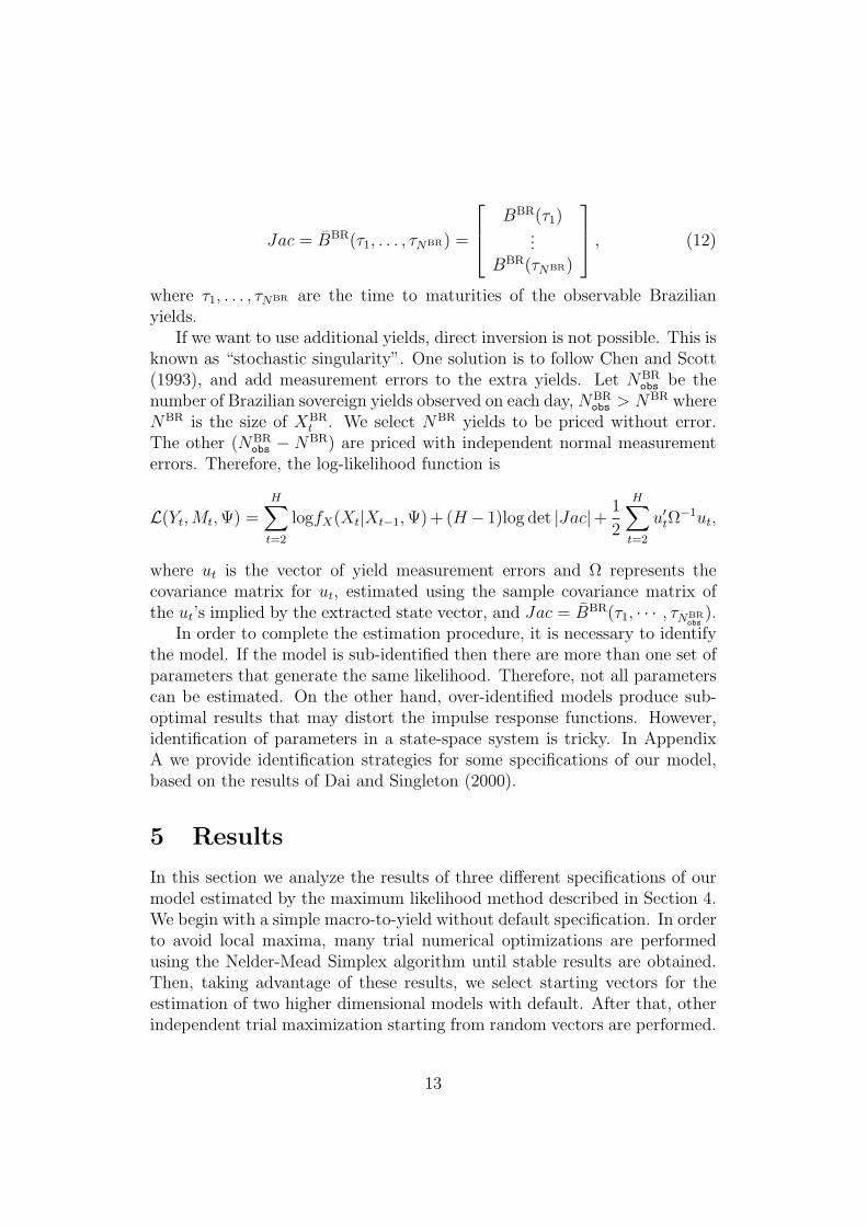
If we want to use additional yields, direct inversion is not possible. This isknown as “stochastic singularity”. One solution is to follow Chen and Scott(1993), and add measurement errors to the extra yields. Let NBR
obs be thenumber of Brazilian sovereign yields observed on each day, NBR
obs > NBR whereNBR is the size of XBR
t . We select NBR yields to be priced without error.The other (NBR
obs − NBR) are priced with independent normal measurementerrors. Therefore, the log-likelihood function is
L(Yt,Mt,Ψ) =H∑t=2
logfX(Xt|Xt−1,Ψ) + (H − 1)log det |Jac|+ 1
2
H∑t=2
u′tΩ−1ut,
where ut is the vector of yield measurement errors and Ω represents thecovariance matrix for ut, estimated using the sample covariance matrix ofthe ut’s implied by the extracted state vector, and Jac = BBR(τ1, · · · , τNBR
obs).
In order to complete the estimation procedure, it is necessary to identifythe model. If the model is sub-identified then there are more than one set ofparameters that generate the same likelihood. Therefore, not all parameterscan be estimated. On the other hand, over-identified models produce sub-optimal results that may distort the impulse response functions. However,identification of parameters in a state-space system is tricky. In AppendixA we provide identification strategies for some specifications of our model,based on the results of Dai and Singleton (2000).
5 Results
In this section we analyze the results of three different specifications of ourmodel estimated by the maximum likelihood method described in Section 4.We begin with a simple macro-to-yield without default specification. In orderto avoid local maxima, many trial numerical optimizations are performedusing the Nelder-Mead Simplex algorithm until stable results are obtained.Then, taking advantage of these results, we select starting vectors for theestimation of two higher dimensional models with default. After that, otherindependent trial maximization starting from random vectors are performed.
13
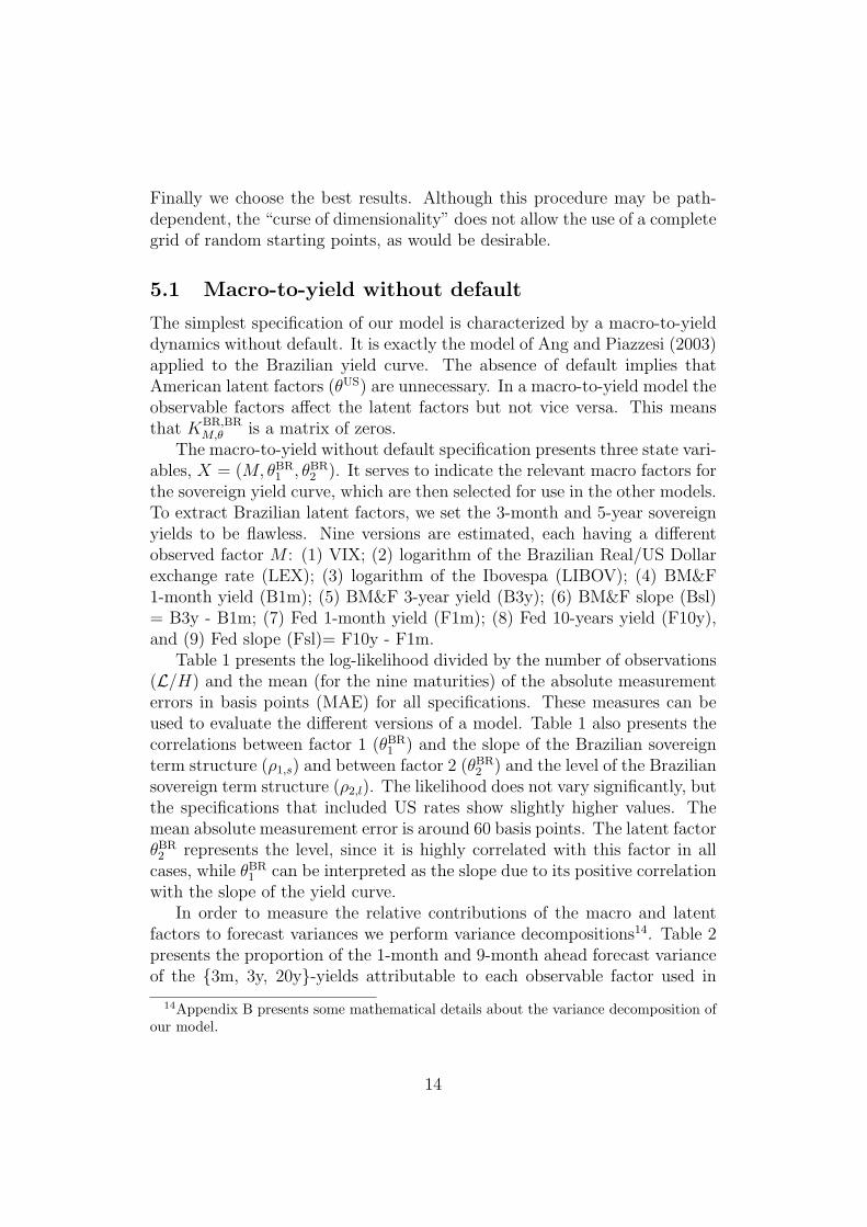
Finally we choose the best results. Although this procedure may be path-dependent, the “curse of dimensionality” does not allow the use of a completegrid of random starting points, as would be desirable.
5.1 Macro-to-yield without default
The simplest specification of our model is characterized by a macro-to-yielddynamics without default. It is exactly the model of Ang and Piazzesi (2003)applied to the Brazilian yield curve. The absence of default implies thatAmerican latent factors (θUS) are unnecessary. In a macro-to-yield model theobservable factors affect the latent factors but not vice versa. This meansthat KBR,BR
M,θ is a matrix of zeros.The macro-to-yield without default specification presents three state vari-
ables, X = (M, θBR1 , θBR
2 ). It serves to indicate the relevant macro factors forthe sovereign yield curve, which are then selected for use in the other models.To extract Brazilian latent factors, we set the 3-month and 5-year sovereignyields to be flawless. Nine versions are estimated, each having a differentobserved factor M : (1) VIX; (2) logarithm of the Brazilian Real/US Dollarexchange rate (LEX); (3) logarithm of the Ibovespa (LIBOV); (4) BM&F1-month yield (B1m); (5) BM&F 3-year yield (B3y); (6) BM&F slope (Bsl)= B3y - B1m; (7) Fed 1-month yield (F1m); (8) Fed 10-years yield (F10y),and (9) Fed slope (Fsl)= F10y - F1m.
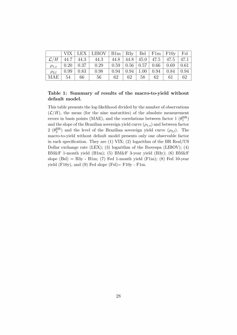
Table 1 presents the log-likelihood divided by the number of observations(L/H) and the mean (for the nine maturities) of the absolute measurementerrors in basis points (MAE) for all specifications. These measures can beused to evaluate the different versions of a model. Table 1 also presents thecorrelations between factor 1 (θBR
1 ) and the slope of the Brazilian sovereignterm structure (ρ1,s) and between factor 2 (θBR
2 ) and the level of the Braziliansovereign term structure (ρ2,l). The likelihood does not vary significantly, butthe specifications that included US rates show slightly higher values. Themean absolute measurement error is around 60 basis points. The latent factorθBR
2 represents the level, since it is highly correlated with this factor in allcases, while θBR
1 can be interpreted as the slope due to its positive correlationwith the slope of the yield curve.
In order to measure the relative contributions of the macro and latentfactors to forecast variances we perform variance decompositions14. Table 2presents the proportion of the 1-month and 9-month ahead forecast varianceof the 3m, 3y, 20y-yields attributable to each observable factor used in
14Appendix B presents some mathematical details about the variance decomposition ofour model.
14
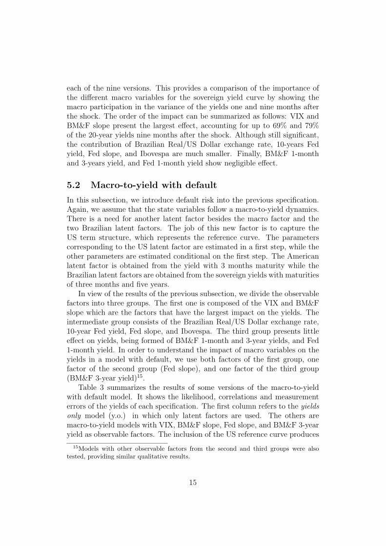
each of the nine versions. This provides a comparison of the importance ofthe different macro variables for the sovereign yield curve by showing themacro participation in the variance of the yields one and nine months afterthe shock. The order of the impact can be summarized as follows: VIX andBM&F slope present the largest effect, accounting for up to 69% and 79%of the 20-year yields nine months after the shock. Although still significant,the contribution of Brazilian Real/US Dollar exchange rate, 10-years Fedyield, Fed slope, and Ibovespa are much smaller. Finally, BM&F 1-monthand 3-years yield, and Fed 1-month yield show negligible effect.
5.2 Macro-to-yield with default
In this subsection, we introduce default risk into the previous specification.Again, we assume that the state variables follow a macro-to-yield dynamics.There is a need for another latent factor besides the macro factor and thetwo Brazilian latent factors. The job of this new factor is to capture theUS term structure, which represents the reference curve. The parameterscorresponding to the US latent factor are estimated in a first step, while theother parameters are estimated conditional on the first step. The Americanlatent factor is obtained from the yield with 3 months maturity while theBrazilian latent factors are obtained from the sovereign yields with maturitiesof three months and five years.
In view of the results of the previous subsection, we divide the observablefactors into three groups. The first one is composed of the VIX and BM&Fslope which are the factors that have the largest impact on the yields. Theintermediate group consists of the Brazilian Real/US Dollar exchange rate,10-year Fed yield, Fed slope, and Ibovespa. The third group presents littleeffect on yields, being formed of BM&F 1-month and 3-year yields, and Fed1-month yield. In order to understand the impact of macro variables on theyields in a model with default, we use both factors of the first group, onefactor of the second group (Fed slope), and one factor of the third group(BM&F 3-year yield)15.
Table 3 summarizes the results of some versions of the macro-to-yieldwith default model. It shows the likelihood, correlations and measurementerrors of the yields of each specification. The first column refers to the yieldsonly model (y.o.) in which only latent factors are used. The others aremacro-to-yield models with VIX, BM&F slope, Fed slope, and BM&F 3-yearyield as observable factors. The inclusion of the US reference curve produces
15Models with other observable factors from the second and third groups were alsotested, providing similar qualitative results.
15
a gain in likelihood and in fit, because the measurement errors are lower.The latent factor θ2 remains highly linked to the level of the sovereign yields.
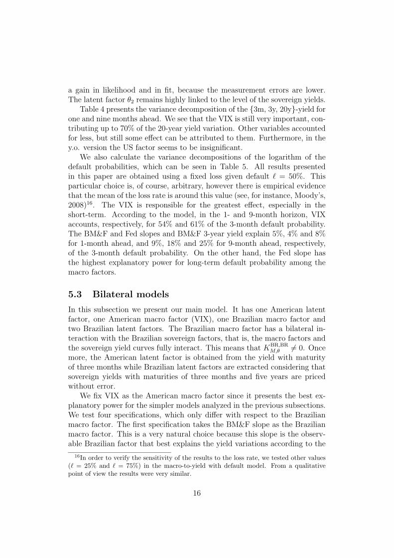
Table 4 presents the variance decomposition of the 3m, 3y, 20y-yield forone and nine months ahead. We see that the VIX is still very important, con-tributing up to 70% of the 20-year yield variation. Other variables accountedfor less, but still some effect can be attributed to them. Furthermore, in they.o. version the US factor seems to be insignificant.
We also calculate the variance decompositions of the logarithm of thedefault probabilities, which can be seen in Table 5. All results presentedin this paper are obtained using a fixed loss given default ` = 50%. Thisparticular choice is, of course, arbitrary, however there is empirical evidencethat the mean of the loss rate is around this value (see, for instance, Moody’s,2008)16. The VIX is responsible for the greatest effect, especially in theshort-term. According to the model, in the 1- and 9-month horizon, VIXaccounts, respectively, for 54% and 61% of the 3-month default probability.The BM&F and Fed slopes and BM&F 3-year yield explain 5%, 4% and 8%for 1-month ahead, and 9%, 18% and 25% for 9-month ahead, respectively,of the 3-month default probability. On the other hand, the Fed slope hasthe highest explanatory power for long-term default probability among themacro factors.
5.3 Bilateral models
In this subsection we present our main model. It has one American latentfactor, one American macro factor (VIX), one Brazilian macro factor andtwo Brazilian latent factors. The Brazilian macro factor has a bilateral in-teraction with the Brazilian sovereign factors, that is, the macro factors andthe sovereign yield curves fully interact. This means that KBR,BR
M,θ 6= 0. Oncemore, the American latent factor is obtained from the yield with maturityof three months while Brazilian latent factors are extracted considering thatsovereign yields with maturities of three months and five years are pricedwithout error.
We fix VIX as the American macro factor since it presents the best ex-planatory power for the simpler models analyzed in the previous subsections.We test four specifications, which only differ with respect to the Brazilianmacro factor. The first specification takes the BM&F slope as the Brazilianmacro factor. This is a very natural choice because this slope is the observ-able Brazilian factor that best explains the yield variations according to the
16In order to verify the sensitivity of the results to the loss rate, we tested other values(` = 25% and ` = 75%) in the macro-to-yield with default model. From a qualitativepoint of view the results were very similar.
16
macro-to-yields models. The second use the logarithm of the Ibovespa in USDollars. This variable combines in single factor the information of two sourcesof uncertainty that present fairly good explanatory power in the macro-to-yield without default framework. Finally, although Brazilian domestic yieldspresent little effect, we consider the 3-month and 3-year Brazilian yields asdomestic factors just to implement a robustness test.
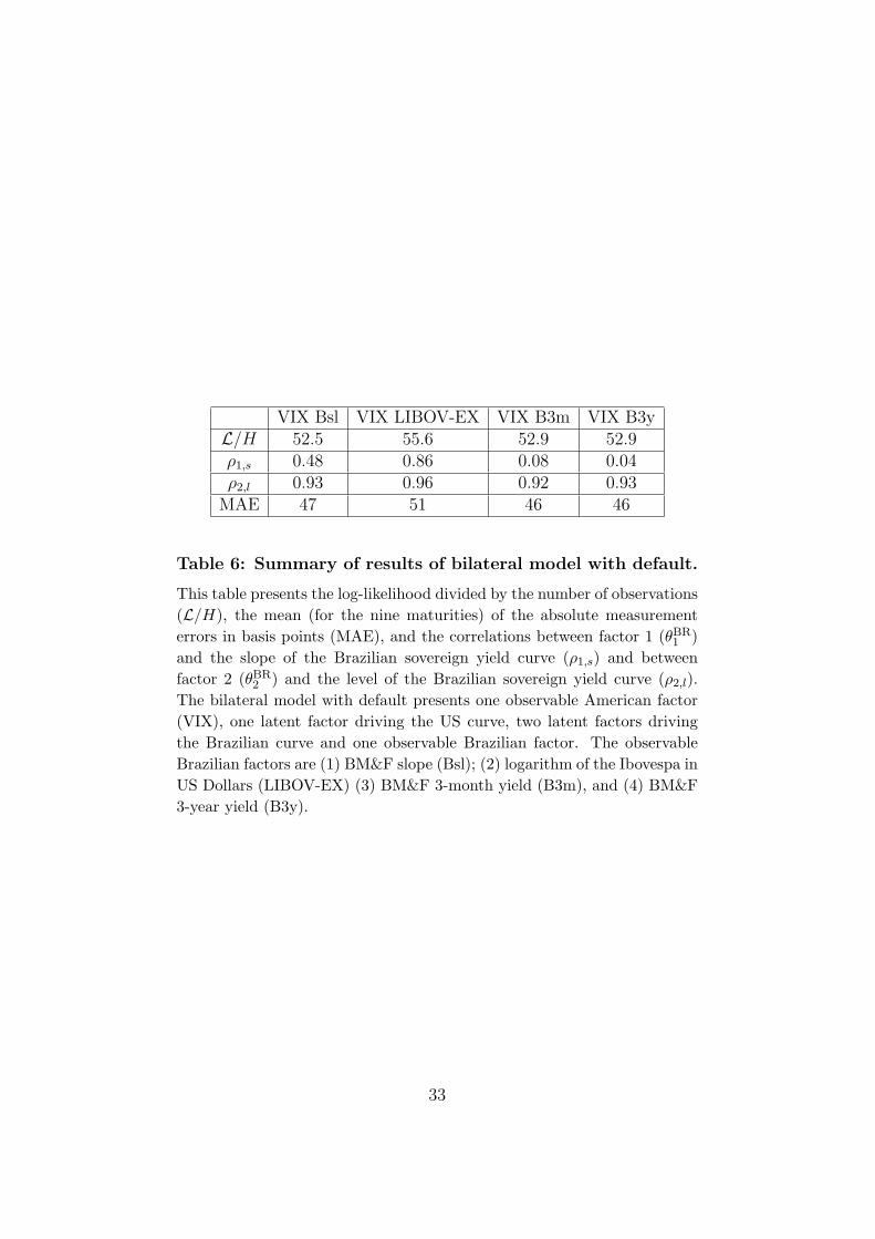
Table 6 contains statistical measures of some versions of the bilateralmodel. Their likelihoods have increased in relation to the previous models,which indicates that the second macro factor and the bilateral dynamics addinformation and improve the in-sample fit, with the specification containingthe Ibovespa presenting slightly higher likelihood. Also, the mean measure-ment errors of yields decreased to about 50 basis points. The unobservablefactor θ2 can still be interpreted as the level of the sovereign curve, but θ1 isin some cases uncorrelated to the slope.
Table 7 reports the variance decomposition of 1m, 3y, 20y-yields forforecast horizons of one and nine months ahead. In line with the preliminarymodels, the VIX is again the most important macro factor influencing theyields. The effect is stronger on the long end of the curve. Among thedomestic variables, only the BM&F slope presents significant explanatorypower. Note that the latent factor related with the level of the sovereigncurve is responsible for a large amount of yield variations. This suggeststhe existence of idiosyncratic sources of uncertainty in the sovereign yieldcurve that are not explained by the observable factors used in our model.This result is in agreement with the findings of Ang and Piazzesi (2003) andDiebold et al. (2006).
Table 8 presents the variance decomposition of the default probabilities.We now analyze in more details the 9-month horizon decomposition, sincein this case the effect of the initial condition is attenuated. Note that inall specifications, the US latent factor (approximately the Fed short rate)shows almost no effect on short-term default probabilities. However, for thelong-term (20 years), it is the principal factor, explaining around 80% ofchanges of implied default probabilities nine months ahead. The effect ofthe VIX is smaller over the long-term, but about 50% of changes in impliedshort-term default probabilities are attributable to changes in this observablefactor. Among the domestic factors, only the slope of the Brazilian local termstructure has a relatively important effect, accounting for 11% of changes inimplied short-term default probabilities. Thus, we can conclude that, givenour model and sample, the domestic rates, and also the Ibovespa are notrelevant sources driving default probability movements.
Figure 3 compares the evolution of the 1-year survival probabilities (oneminus default probabilities) over the sample period. It can be seen that
17

changing the domestic macro factor does not significantly alter the probabil-ities. Observe that all versions capture the Brazilian electoral crisis in thesecond half of 2002, with the y.o. model having the largest impact on survivalprobability. The 1-year ahead survival probabilities fell from an average of85% to around 70%, recovering later to around 90%.
In order to gauge the response of yields due to an unexpected change instate variables, we calculate impulse response functions17. Figures 4, 5 and6 show the effect of a shock to US latent factor (θUS
1 ), VIX and observabledomestic factors (BM&F yields and slope and Ibovespa in US Dollars), re-spectively, on the Brazilian 3m, 3y, 20y-yields up to 18-months after theshock. The size of the shock is one standard deviation of a monthly variationof a state variable. In the next three months after a shock on VIX, yieldsrise about 1% and then fall. Changes in either the domestic short or longrate do not result in changes of the sovereign yields. The same is true forthe domestic stock exchange index (Ibovespa). However, a positive BM&Fslope shock causes an increase in the yields. This may indicate a change ofexpectations of a future rise in inflation.
We now turn to survival probabilities. Figures 7, 8, 9 show the impact of aone deviation increase of a monthly variation of the US latent factor, VIX andobservable domestic factors, respectively, on the survival probabilities in thenext three months, three years and twenty years. It shows that the survivalprobability falls by up to 4% in relative terms due to a shock in the Fed shortrate. An increase in VIX also decreases the survival probability about 1.5%in relative terms. Among the domestic factors, only the BM&F slope hassome impact, decreasing the long-term survival probability by about 0.7% inrelative terms.
6 Conclusion
We proposed a model that combines an affine yield dynamics with macrofactors and credit risk. The model was estimated in two steps using the USand Brazilian sovereign yield curves. The credit spreads, the macro factorsand the US yield curve have contemporaneous and lagged interaction. Wewere able to test how selected domestic and external macro factors such asthe Brazilian Real/US Dollar exchange rate, VIX (volatility index of S&P),Ibovespa (Sao Paulo stock exchange index) and domestic yield curve influ-ence the spreads and default probabilities. The model was identified beforemaking restrictions motivated by economic assumptions. Our findings indi-
17Appendix B presents some results concerning the impulse response functions appliedto our model.
18

cate that the VIX and US yield curve are the most important factors drivingthe Brazilian sovereign term structure and default probabilities. This resultis consistent with the fact that credit risk premia of sovereign bond are highlycorrelated with the US economic conditions. The VIX has a high impact on20-year bond yields and on short-term default probabilities, while the fedfund rate has high explanatory power on the long-term default probabili-ties. Among the domestic factors, only the slope of the local yield curveshows a significant effect on the Brazilian credit spread. However, a signif-icant portion of variations in yields and default probabilities are explainedby an unobservable factor highly correlated with the level of the Braziliansovereign curve. Due to lack of an extensive historical dataset, we estimateda continuous-time version with daily observations, which limited the choicesof macro variables. Future work can test monthly models, allowing the use ofimportant variables such as Central Bank reserves, real activity and inflation.
19
Appendix A - Model identification
Here, we show how to identify the parameters of a Gaussian affine modelwith macro factors and credit spreads. This approach is based on the studyof Dai and Singleton (2000).
First we consider the default-free case. Suppose there are p macro vari-ables M and q latent variables θ. The vector X = (M, θ) follows a Gaussianaffine dynamics:
dXt =
[dMt
dθt
]=
[KM,M KM,θ
Kθ,M Kθ,θ
]([ξMξθ
]−[Mt
θt
])dt
+
[ΣM,M ΣM,θ
Σθ,M Σθ,θ
] [dW P
M(t)dW P
θ (t)
]= K(ξ −Xt)dt+ ΣdW P(t). (13)
The instantaneous short-term rate is given by rt = δ0 + δ1 · Xt while themarket price of risk obeys Equation 6. Hence, the dynamics of X in the risk-neutral measure is dX = K?(ξ?−Xt)dt+ ΣdWQ(t) and the yield curve is anaffine function of X, Yt(τ) = A(τ) + BM(τ)Mt + Bθ
t (τ)θ = A(τ) + B(τ)Xt.The parameter vector is denoted by Ψ = (δ0, δ1, K, ξ, λ0, λ1,Σ).
Some of the above parameters must be arbitrarily fixed, otherwise thereare multiple solutions to the estimation problem since we can define operatorsthat preserve the likelihood as shown below.
Let L ∈ R(p+q)×(p+q) be a non-singular matrix and v ∈ Rp+q a vector suchthat
L =
(I 0α β
)and v =
(0vθ
),
where I ∈ Rp×p is the identity matrix, α ∈ Rq×p, β ∈ Rq×q, and vθ ∈ Rq.Consider the following maps:
TL,vΨ, X =(δ0 − δ′1L−1v, (L′)−1δ1, LKL
−1, v + Lξ, λ0 − λ1L−1v, λ1L
−1, LΣ), LX + v(14)
andTOΨ, X = (δ0, δ1, K, ξ, λ0, λ1,ΣO
′), X, (15)
where O ∈ R(p+q)×(p+q) is a rotation matrix.
Proposition 1 The operators TL,v and TO preserve the likelihood of theaffine model defined above under the Chen-Scott (1993) estimation procedure.
Proof
20

The log-likelihood L of the affine model under the Chen-Scott (1993)inversion is
L(Ψ, X) = logfY (Yt1 , ..., YtH |Ψ, X) =
logfX(Xt1 , ..., XtH |Ψ) + logfu(ut1,...,utH ) + log| det Jac|H−1 =
(H − 1)log| det Bθ|+∑H
t=2 logfXt|Xt−1(Xt|Ψ) + logfu(ut) =
(H − 1)log| det Bθ| − 12(H − 1)log det
[∆t(e−K∆t
)ΣΣ′
(e−K∆t
)′]+∑H
t=2 logfu(ut)− 12
∑Ht=2(Xt − µ)′
[∆t(e−K∆t
)ΣΣ′
(e−K∆t
)′]−1
(Xt − µ),
where µ = e−K∆tξ + (1 − e−K∆tξ)Xt−1, ∆t = ti − ti−1 ∀i, H is the sam-ple size, and Bθ(·) is evaluated at the time to maturities of yields withoutmeasurement errors (see Equation 12).
We begin by proving that L(Ψ, X) = L(TL,v(Ψ, X)). The strategy of theproof is to analyze what happens with each of the four terms of the log-likelihood when the operator TL,v is applied. First, note that the expressionunder the last summation symbol is preserved. The transformation of µ is
µ(TL,v(Ψ, X)) = e−LKL−1∆tLξ +
(1− e−LKL
−1∆t)LXt−1 =
Le−K∆tL−1Lξ + (1− Le−K∆tL−1)LXt−1 = Lµ.
Then, applying TL,v on the last summation expression of the log-likelihood,we have
(LXt − Lµ)′[(
e−LKL−1∆tLΣ
√∆t)(
e−LKL−1∆tLΣ
√∆t)′]−1
(LXt − Lµ)
= (Xt − µ)′L′[(Le−K∆tL−1LΣ
√∆t)(
Le−K∆tL−1LΣ√
∆t)′]−1
L(Xt − µ)
= (Xt − µ)′L′[L′−1
(e−K∆tΣ
√∆t)′−1 (
e−K∆tΣ√
∆t)−1
L−1
]L(Xt − µ)
= (Xt − µ)′[(
e−K∆tΣ√
∆t)′−1 (
e−K∆tΣ√
∆t)−1]
(Xt − µ).
21

The second term of the log-likelihood changes to
−12(H − 1)log det
[(e−LKL
−1∆tLΣ√
∆t)(
e−LKL−1∆tLΣ
√∆t)′]
=
−12(H − 1)
log det
[(e−K∆tΣ
√∆t)(
e−K∆tΣ√
∆t)′]
+ 2log detL
=
−12(H − 1)[log det
[(e−K∆tΣ
√∆t)(
e−K∆tΣ√
∆t)′]− (H − 1)log detL.
(16)It is easy to see that
(H − 1)log| det Bθ| (TL,v(Ψ, X)) = (H − 1)log| det β−1Bθ|
= (H − 1)log| det Bθ|+ (H − 1)log| det β−1|.
Since detL = det β, the last term that appeared in (16) cancels out with thelast term in the expression above.
Moreover, it is also easy to see that ut does not change under the trans-formation TL,v.
Finally, L(Ψ, X) = L(TO(Ψ, X)) since the only expression affected by therotation is preserved:[(
e−K∆tΣO′√
∆t)(
e−K∆tΣO′√
∆t)′]−1
=
[(e−K∆tΣ
√∆t)(
e−K∆tΣ√
∆t)′]−1
.
2
Therefore, there are infinite parameter vectors with the same likelihood.Hence, before estimation through the maximum likelihood method, some pa-rameters must be fixed. On the other hand, the imposition of over-identifyingrestrictions may produce sub-optimal results that distort the impulse re-sponse functions. The model can be considered identified if all the degreesof freedom of the model, which are given by α, β, vθ and O, are eliminated.
Note that vθ can always be used to set ξθ = 0. In addition, the rotationO implies that Σ must be a triangular matrix for a given state vector order.Hence, we choose Σθ,θ and ΣM,M to be lower triangular and ΣM,θ = 0. Finally,α and β can be set so that Σθ,θ = I , ΣM,θ = 0, and Kθ,θ is lower triangular.This completes the identification of the default-free case.
22

We now turn to the case with default. Formally speaking, the reducedcredit risk model of Duffie and Singleton (1999) is simply a higher-dimensionalaffine model and the same identification procedure can be applied. There are,however, two subtleties involved.
The first is that there are natural restrictions that can be placed to thedefault model coming from economic considerations. For instance, we haveconsidered that the American yield curve and macro factors affect the Brazil-ian curve, but not vice versa. However, the model must be first identifiedfrom the econometric point of view before additional restrictions are imposed,otherwise the same parameters might be fixed twice, leaving unresolved de-grees of freedom.
The second point is that in the default-free case was illustrated supposingthat the macro factors are “more endogenous” than the latent factors. Inthe default case, X = (θUS,MUS,MBR, θBR), thus the American latent fac-tors come before the Brazilian factors, which would in principle change theoperator TL,v and consequently the degrees of freedom. The other inversion,namely the American macro vector coming after the latent vector, is due tothe fact that only the VIX is considered and it does not interfere with theidentification procedure.
However, since we use a two-step procedure, the parameters and statefactors related to the American term structure are estimated first. So, wecan think of the American latent factors as if they were “macro” factors andproceed to the identification considering that MBR = (θUS,MUS,MBR) is infact the macro vector for the default case.
In summary, the economic restrictions impose that δr1 = (δr,US1 , 0) and
that the matrix K is block-triangular, which means that Brazilian factors donot affect American factors. Therefore the identified Σ is given by:
(ΣMM 0
0 I
), where ΣMM =
I 0 0
0 ΣUS,USM,M 0
ΣBR,USM,θ ΣBR,US
M,M ΣBR,BRM,M
.
Appendix B - Impulse Response and Variance
Decomposition
One way to evaluate the impact of macro shocks on the term structure ofinterest rates and default probabilities is through impulse response functions(IRF) and variance decompositions (VD). In continuous time, the evolution
23

of the state vector is given by
Xti|ti−k= e−K(ti−ti−k)Xi−k +
k−1∑l=0
∫ ti−k+l+1
ti−k+l
e−K(ti−u)ΣdW Pu .
The stochastic integral is Gaussian with zero mean and variance
E
[∫ ti
ti−1
e−K(ti−u)ΣdW Pu
]2
=
∫ ti
ti−1
e−K(ti−u)ΣΣ′(e−K(ti−u))′du. (17)
When ∆t = ti−ti−1 is small, the variance is approximately e−K∆tΣΣ′(e−K∆t)′∆t.Hence, the response of Xt to a shock εt in a time interval of ∆t is
Σ√
∆tεt e−K∆tΣ√
∆tεt e−2K∆tΣ√
∆tεt e−3K∆tΣ√
∆tεt ...t+ 0 t+ 1 t+ 2 t+ 3 ...
(18)
Similarly, the response of the yield Yt = A+BXt is given by
BΣ√
∆tεt Be−K∆tΣ√
∆tεt Be−2K∆tΣ√
∆tεt Be−3K∆tΣ√
∆tεt ...t+ 0 t+ 1 t+ 2 t+ 3 ...
(19)and the response of the logarithm of the survival probability, log Pr(t, τ) =aPr + bPrXt, is
bPrΣ√
∆tεt bPre−K∆tΣ√
∆tεt bPre−2K∆tΣ√
∆tεt bPre−3K∆tΣ√
∆tεt ...t+ 0 t+ 1 t+ 2 t+ 3 ...
(20)In Section 5 we work with a shock of one standard deviation of a monthly
variation of a factor. This means that√
∆t =√
21/252 considering a 252day-year.
To find the variance decomposition, we must calculate the mean squarederror (MSE) of h-periods ahead error Xt+h − EXt+h|t:
MSE =
∫ t+h
t
e−K(t+h−u)ΣΣ′(e−K(t+h−u))′du.
Hence, the contribution corresponding to the jth factor in the variance de-composition of Xt+h, Yt+h(τ) and log Pr(t+ h, τ) at time t are
V Dj(X) =∫ t+ht
e−K(t+h−u)ΣjΣ′j(e−K(t+h−u))′du,
V Dj(Y ) = B′(τ)(∫ t+h
te−K(t+h−u)ΣjΣ
′j(e−K(t+h−u))′du
)B(τ),
V Dj(log Pr) = bPr′(τ)(∫ t+h
te−K(t+h−u)ΣjΣ
′j(e−K(t+h−u))′du
)bPr(τ).
(21)
24

References
[1] Almeida, C. and J. Vicente (2009). Identifying volatility risk premiafrom fixed income Asian options. Journal of Banking & Finance, 33,pp. 652-661.
[2] Ang, A. and M. Piazzesi (2003). A no-arbitrage vector autoregressionof term structure dynamics with macroeconomic and latent variables,Journal of Monetary Economics, 50, pp. 745-787.
[3] Ang, A., S. Dong, and M. Piazzesi (2007). No-arbitrage Taylor rules,NBER Working paper 13448.
[4] Berndt, A., R. Douglas, D. Duffie, M. Ferguson, and D. Schranzk (2004).Measuring default risk premia from default swap rates and EDFs. Work-ing Paper, Stanford University.
[5] Black, F. and J. Cox (1976). Valuing corporate securities: some effectsof bond indenture provisions, Journal of Finance, 31 (2), pp. 351-367.
[6] Black, F. and M. Scholes (1973). The pricing of options and corporateliabilities, Journal of Political Economy, 81 (3), pp. 637-654.
[7] Chen, R. and L. Scott (1993). Maximum likelihood estimation for amulti-factor equilibrium model of the term structure of interest rates,Journal of Fixed Income, 3 (4), pp. 14-31.
[8] Dai, Q. and K. Singleton (2000). Specification analysis of affine termstructure models, Journal of Finance, 55, pp. 1943-1978.
[9] Dai, Q. and K. Singleton (2002). Expectation puzzles, time-varying riskpremia, and affine models of the term structure. Journal of FinancialEconomics, 63, pp. 415-441.
[10] Diebold, F., G. Rudebusch and S. Aruoba (2006). The macroeconomyand the yield curve: a dynamic latent factor approach. Journal of Econo-metrics, 131, pp. 309-338.
[11] Duffee, G. (2002). Term premia and interest rates forecasts in affinemodels. Journal of Finance, 57, pp. 405-443.
[12] Duffie, D. (2001) Dynamic asset pricing theory, Third edition, PrincetonUniversity Press.
25

[13] Duffie, D. and R. Kan (1996) A yield-factor model of interest rates,Mathematical Finance, 6, pp. 379-406.
[14] Duffie, D., L. Pedersen and K. Singleton (2003). Modeling sovereignyield spreads: a case study of Russian debt, Journal of Finance, 58, pp.119-159.
[15] Duffie, D. and K. Singleton (1999). Modeling term structures of default-able bonds, Review of Financial Studies, 12, pp. 687-720.
[16] Fackler, P. (2000). Moments of affine diffusions, Working paper, NorthCarolina State University.
[17] Giesecke, K. (2004). Credit risk modeling and valuation: an introduc-tion, in Credit Risk Models and Management, Vol. 2, Ed. D. Shimko,Riskbooks.
[18] Hordal, P., O. Tristani, and D. Vestin. (2006). A Joint EconometricModel of Macroeconomic and Term Structure Dynamics. Journal ofEconometrics, 127, pp. 405-44.
[19] Goldman Sachs Global Economics Department (2007). BRICs and be-yond.
[20] Lando, D. (1998). On Cox processes and credit risky bonds, Review ofDerivatives Research, 2(2), pp. 99-120.
[21] Leland, H. (1994). Risky debt, bond covenants and optimal capital struc-ture, Journal of Finance, 49 (4), pp. 1213-1252.
[22] Litterman, R. and J. Scheinkman (1991). Common factors affectingbond returns, Journal of Fixed Income 1, pp. 54-61.
[23] Moody’s (2008). Sovereign default and recovery rates, 1983-2007,Working Paper, Moody’s Global Credit Research. Available athttp://www.moodys.com/.
[24] Merton, R. (1974). On the pricing of corporate debt: the risk structureof interest rates, Journal of Finance 29 (2), pp. 449-470.
[25] Moreira, A. and K. Rocha (2004). Two-factor structural model of deter-minants of Brazilian sovereign risk, Journal of Fixed Income, 14 (2).
[26] Pan, J. and K. Singleton (2008). Default and recovery implicit in theterm structure of sovereign CDS spreads. Journal of Finance, 63 (5),pp. 2345-2384.
26
[27] Pericoli, M. and M. Taboga (2008). Canonical term-structure modelswith observable factors and the dynamics of bond risk premia, Journalof Money, Credit and Banking, 40 (7), pp. 1471-1488.
[28] Rudebusch, G. and T. Wu (2004). A Macro-finance model of the termstructure, monetary policy, and the economy. Proceedings of the FederalReserve Bank of San Francisco.
[29] Schonbucher, P. (2003).Credit derivatives pricing models, Wiley Finance.
[30] Shiryaev, A. (1995). Probability, Springer Verlag.
[31] Spencer, P. (2008). Stochastic volatility in a macro-finance model of theU.S. term structure of interest rates 1961-2004. Journal of Money, Creditand Banking, 40 (6), pp. 1177-1215.
[32] Xu, D. and P. Ghezzi, (2002). From fundamentals to spreads: A fairspread model for high yield emerging market sovereigns, Deutsche BankGlobal Markets Research.
27
VIX LEX LIBOV B1m B3y Bsl F1m F10y FslL/H 44.7 44.3 44.3 44.8 44.8 45.0 47.5 47.5 47.1ρ1,s 0.20 0.37 0.29 0.59 0.56 0.57 0.66 0.69 0.61ρ2,l 0.99 0.83 0.98 0.94 0.94 1.00 0.94 0.84 0.94
MAE 54 66 56 62 62 58 62 61 62
Table 1: Summary of results of the macro-to-yield withoutdefault model.
This table presents the log-likelihood divided by the number of observations(L/H), the mean (for the nine maturities) of the absolute measurementerrors in basis points (MAE), and the correlations between factor 1 (θBR
1 )and the slope of the Brazilian sovereign yield curve (ρ1,s) and between factor2 (θBR
2 ) and the level of the Brazilian sovereign yield curve (ρ2,l). Themacro-to-yield without default model presents only one observable factorin each specification. They are (1) VIX; (2) logarithm of the BR Real/USDollar exchange rate (LEX); (3) logarithm of the Ibovespa (LIBOV); (4)BM&F 1-month yield (B1m); (5) BM&F 3-year yield (B3y); (6) BM&Fslope (Bsl) = B3y - B1m; (7) Fed 1-month yield (F1m); (8) Fed 10-yearyield (F10y), and (9) Fed slope (Fsl)= F10y - F1m.
28

Yields1-month ahead
VIX LEX LIBOV B1m B3y Bsl F1m F10y Fsl3m 15 7 1 0 0 16 0 0 03y 23 9 0 0 0 23 0 4 020y 54 9 6 0 0 50 0 8 0
Yields9-months ahead
VIX LEX LIBOV B1m B3y Bsl F1m F10y Fsl3m 31 7 22 0 0 46 0 0 63y 46 11 13 0 0 61 0 10 720y 69 14 21 0 0 79 0 16 7
Table 2: Variance decompositions of the macro-to-yield with-out default model.This table presents the proportion (in percent) of the 1-month and 9-monthahead forecast variance of the 3m, 3y, 20y-yields attributable to each ob-servable factor. The macro-to-yield without default model presents onlyone observable factor in each specification. They are (1) VIX; (2) loga-rithm of the BR Real/US Dollar exchange rate (LEX); (3) logarithm ofthe Ibovespa (LIBOV); (4) BM&F 1-month yield (B1m); (5) BM&F 3-yearyield (B3y); (6) BM&F slope (Bsl) = B3y - B1m; (7) Fed 1-month yield(F1m); (8) Fed 10-year yield (F10y), and (9) Fed slope (Fsl)= F10y - F1m.
29

y.o. VIX Bsl Fsl B3yL/H 42.1 47.0 48.2 49.9 47.8ρ1,s 0.28 0.37 0.42 -0.17 0.19ρ2,l 0.99 0.97 0.98 0.96 0.86
MAE 68 53 50 59 54
Table 3: Summary of results of the macro-to-yield with de-fault model.
This table presents the log-likelihood divided by the number of observations(L/H), the mean (for the nine maturities) of the absolute measurementerrors in basis points (MAE), and the correlations between factor 1 (θBR
1 )and the slope of the Brazilian sovereign yield curve (ρ1,s) and betweenfactor 2 (θBR
2 ) and the level of the Brazilian sovereign yield curve (ρ2,l). Themacro-to-yield with default model presents one observable factor, one latentfactor driving the US curve and two latent factors driving the Braziliancurve. The observable factors are (1) VIX; (2) BM&F slope (Bsl) = B3y -B1m, (3) Fed slope (Fsl)= F10y - F1m, and (4) BM&F 3-year yield (B3y).The y.o. model refers to a specification in which only yields are used, thatis, a specification without observable factors.
30
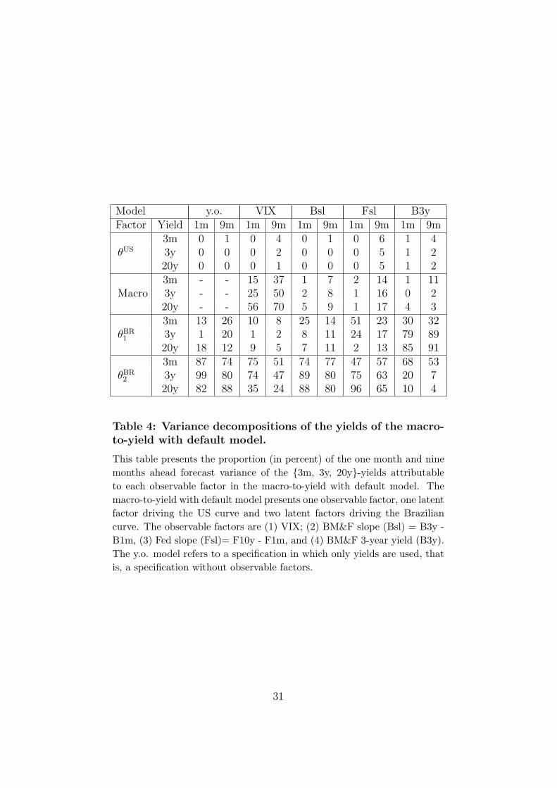
Model y.o. VIX Bsl Fsl B3yFactor Yield 1m 9m 1m 9m 1m 9m 1m 9m 1m 9m
θUS
3m 0 1 0 4 0 1 0 6 1 43y 0 0 0 2 0 0 0 5 1 220y 0 0 0 1 0 0 0 5 1 2
Macro3m - - 15 37 1 7 2 14 1 113y - - 25 50 2 8 1 16 0 220y - - 56 70 5 9 1 17 4 3
θBR1
3m 13 26 10 8 25 14 51 23 30 323y 1 20 1 2 8 11 24 17 79 8920y 18 12 9 5 7 11 2 13 85 91
θBR2
3m 87 74 75 51 74 77 47 57 68 533y 99 80 74 47 89 80 75 63 20 720y 82 88 35 24 88 80 96 65 10 4
Table 4: Variance decompositions of the yields of the macro-to-yield with default model.
This table presents the proportion (in percent) of the one month and ninemonths ahead forecast variance of the 3m, 3y, 20y-yields attributableto each observable factor in the macro-to-yield with default model. Themacro-to-yield with default model presents one observable factor, one latentfactor driving the US curve and two latent factors driving the Braziliancurve. The observable factors are (1) VIX; (2) BM&F slope (Bsl) = B3y -B1m, (3) Fed slope (Fsl)= F10y - F1m, and (4) BM&F 3-year yield (B3y).The y.o. model refers to a specification in which only yields are used, thatis, a specification without observable factors.
31
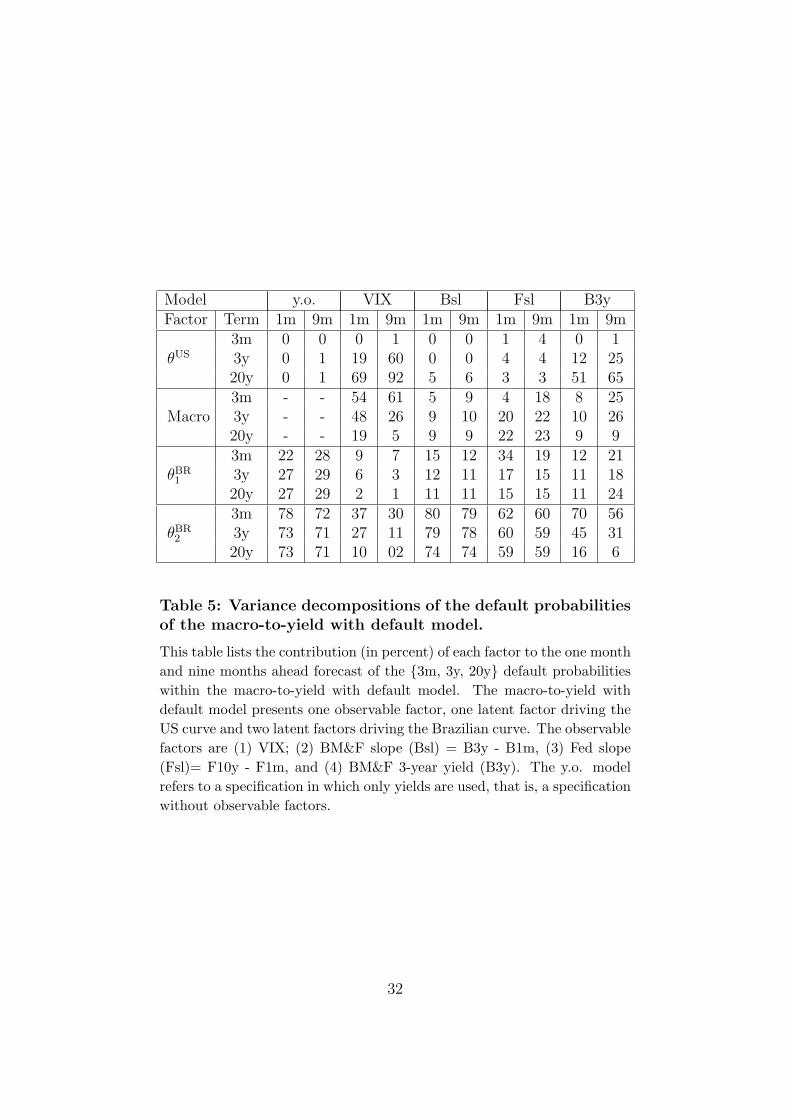
Model y.o. VIX Bsl Fsl B3yFactor Term 1m 9m 1m 9m 1m 9m 1m 9m 1m 9m
θUS
3m 0 0 0 1 0 0 1 4 0 13y 0 1 19 60 0 0 4 4 12 2520y 0 1 69 92 5 6 3 3 51 65
Macro3m - - 54 61 5 9 4 18 8 253y - - 48 26 9 10 20 22 10 2620y - - 19 5 9 9 22 23 9 9
θBR1
3m 22 28 9 7 15 12 34 19 12 213y 27 29 6 3 12 11 17 15 11 1820y 27 29 2 1 11 11 15 15 11 24
θBR2
3m 78 72 37 30 80 79 62 60 70 563y 73 71 27 11 79 78 60 59 45 3120y 73 71 10 02 74 74 59 59 16 6
Table 5: Variance decompositions of the default probabilitiesof the macro-to-yield with default model.
This table lists the contribution (in percent) of each factor to the one monthand nine months ahead forecast of the 3m, 3y, 20y default probabilitieswithin the macro-to-yield with default model. The macro-to-yield withdefault model presents one observable factor, one latent factor driving theUS curve and two latent factors driving the Brazilian curve. The observablefactors are (1) VIX; (2) BM&F slope (Bsl) = B3y - B1m, (3) Fed slope(Fsl)= F10y - F1m, and (4) BM&F 3-year yield (B3y). The y.o. modelrefers to a specification in which only yields are used, that is, a specificationwithout observable factors.
32
VIX Bsl VIX LIBOV-EX VIX B3m VIX B3yL/H 52.5 55.6 52.9 52.9ρ1,s 0.48 0.86 0.08 0.04ρ2,l 0.93 0.96 0.92 0.93
MAE 47 51 46 46
Table 6: Summary of results of bilateral model with default.
This table presents the log-likelihood divided by the number of observations(L/H), the mean (for the nine maturities) of the absolute measurementerrors in basis points (MAE), and the correlations between factor 1 (θBR
1 )and the slope of the Brazilian sovereign yield curve (ρ1,s) and betweenfactor 2 (θBR
2 ) and the level of the Brazilian sovereign yield curve (ρ2,l).The bilateral model with default presents one observable American factor(VIX), one latent factor driving the US curve, two latent factors drivingthe Brazilian curve and one observable Brazilian factor. The observableBrazilian factors are (1) BM&F slope (Bsl); (2) logarithm of the Ibovespa inUS Dollars (LIBOV-EX) (3) BM&F 3-month yield (B3m), and (4) BM&F3-year yield (B3y).
33

Model VIX Bsl VIX LIBOV-EX VIX B3m VIX B3yFactor Yield 1m 9m 1m 9m 1m 9m 1m 9m
θUS
3m 0 2 1 3 1 2 1 33y 0 1 0 5 0 1 0 120y 0 0 0 4 0 0 0 0
MUS
3m 2 20 2 21 4 26 4 323y 2 23 4 21 5 33 5 3920y 27 38 36 16 20 48 20 53
MBR
3m 2 7 0 0 0 2 1 13y 3 10 0 1 0 2 0 120y 3 9 0 0 0 1 1 2
θBR1
3m 38 22 68 50 76 12 17 93y 13 9 19 52 3 4 2 120y 2 4 5 70 0 1 0 1
θBR2
3m 58 48 29 25 19 57 77 563y 81 57 76 21 91 61 93 5820y 67 49 59 9 80 50 79 43
Table 7: Variance decompositions of the yields of the bilateralmodel with default.
This table presents the proportion (in percent) of the one month and ninemonths ahead forecast variance of the 3m, 3y, 20y-yields attributable toeach observable factor in the bilateral model with default. The bilateralmodel with default presents one observable American factor (VIX), onelatent factor driving the US curve, two latent factors driving the Braziliancurve and one observable Brazilian factor. The observable Brazilian factorsare (1) BM&F slope (Bsl); (2) logarithm of the Ibovespa in US Dollars(LIBOV-EX) (3) BM&F 3-month yield (B3m), and (4) BM&F 3-year yield(B3y).
34

Model VIX Bsl VIX LIBOV-EX VIX B3m VIX B3yFactor Term 1m 9m 1m 9m 1m 9m 1m 9m
θUS
3m 0 0 2 2 0 0 0 03y 7 21 21 59 8 29 9 2920y 47 73 80 93 51 79 52 78
MUS
3m 19 32 16 31 29 42 34 563y 31 31 26 18 36 33 55 5120y 18 11 7 3 20 10 29 16
MBR
3m 8 11 0 0 1 3 1 13y 11 10 1 1 3 3 2 220y 6 3 0 0 1 1 1 1
θBR1
3m 21 12 61 49 11 9 6 33y 11 6 38 16 9 7 1 020y 6 2 10 3 5 2 0 0
θBR2
3m 52 44 22 18 59 46 59 393y 41 31 14 6 43 29 33 1720y 24 11 3 1 23 8 18 5
Table 8: Variance decompositions of the default probabilitiesof bilateral model with default.
This table lists the contribution (in percent) of each factor to the one monthand nine months ahead forecast of the 3m, 3y, 20y default probabilitieswithin the bilateral model with default. The bilateral model with defaultpresents one observable American factor (VIX), one latent factor driving theUS curve, two latent factors driving the Brazilian curve and one observableBrazilian factor. The observable Brazilian factors are (1) BM&F slope(Bsl); (2) logarithm of the Ibovespa in US Dollars (LIBOV-EX) (3) BM&F3-month yield (B3m), and (4) BM&F 3-year yield (B3y).
35
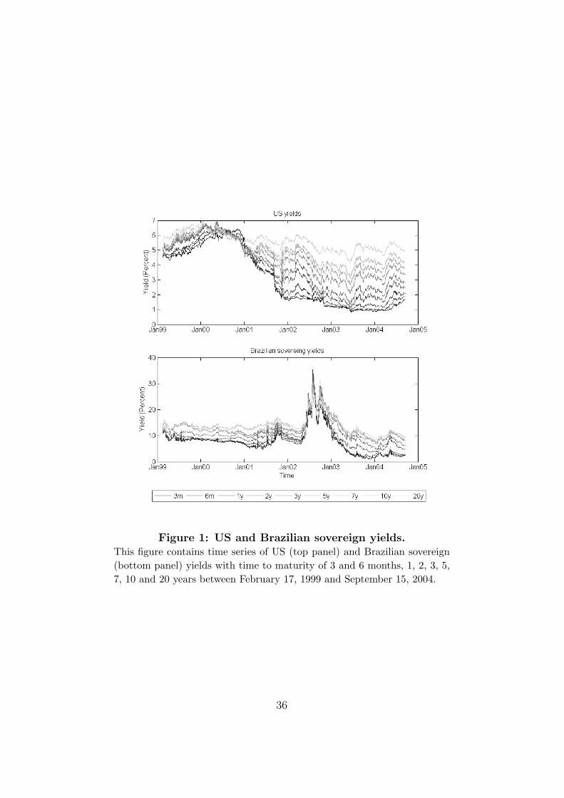
Figure 1: US and Brazilian sovereign yields.This figure contains time series of US (top panel) and Brazilian sovereign(bottom panel) yields with time to maturity of 3 and 6 months, 1, 2, 3, 5,7, 10 and 20 years between February 17, 1999 and September 15, 2004.
36

Figure 2: Observable variables.This figure contains time series of variables used as observable factors in ourmodel between February 17, 1999 and September 15, 2004. The upper leftpanel shows the evolution of the VIX (implied volatility of S&P 500 indexoptions). The upper right panel presents the logarithm of the BrazilianReal/US Dollar exchange rate. The lower left panel presents the logarithmof the Ibovespa, and the lower right panel shows the Brazilian domesticzero-cupon yields with time to maturity of 1, 3 and 36 months.
37

Figure 3: Survival probabilities.This figure shows the 1-year survival probabilities extracted from someversions of the bilateral model and from y.o. model between February 17,1999 and September 15, 2004. The bilateral model with default presentsone observable American factor (VIX), one latent factor driving the UScurve, two latent factors driving the Brazilian curve and one observableBrazilian factor. The observable Brazilian factors are (1) BM&F slope(Bsl); (2) logarithm of the Ibovespa in US Dollars (LIBOV-EX) (3) BM&F3-month yield (B3m), and (4) BM&F 3-year yield (B3y). The y.o. modelrefers to a specification in which only yields are used, that is, a specificationwithout observable factors.
38
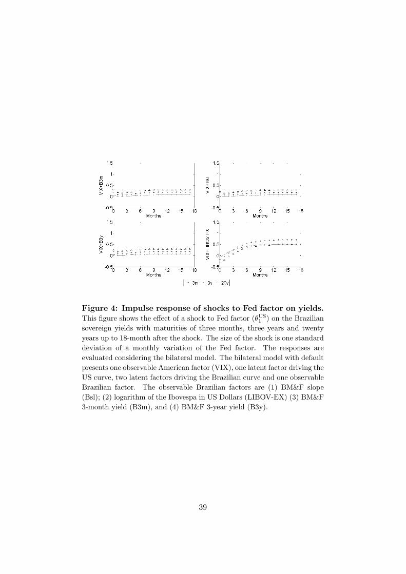
Figure 4: Impulse response of shocks to Fed factor on yields.This figure shows the effect of a shock to Fed factor (θUS
1 ) on the Braziliansovereign yields with maturities of three months, three years and twentyyears up to 18-month after the shock. The size of the shock is one standarddeviation of a monthly variation of the Fed factor. The responses areevaluated considering the bilateral model. The bilateral model with defaultpresents one observable American factor (VIX), one latent factor driving theUS curve, two latent factors driving the Brazilian curve and one observableBrazilian factor. The observable Brazilian factors are (1) BM&F slope(Bsl); (2) logarithm of the Ibovespa in US Dollars (LIBOV-EX) (3) BM&F3-month yield (B3m), and (4) BM&F 3-year yield (B3y).
39

Figure 5: Impulse response of shocks to the VIX on yields.This figure shows the effect of a shock to the VIX on the Brazilian sovereignyields with maturities of three months, three years and twenty years up to18-month after the shock. The size of the shock is one standard deviation ofa monthly variation of the VIX. The responses are evaluated considering thebilateral model. The bilateral model with default presents one observableAmerican factor (VIX), one latent factor driving the US curve, two latentfactors driving the Brazilian curve and one observable Brazilian factor. Theobservable Brazilian factors are (1) BM&F slope (Bsl); (2) logarithm of theIbovespa in US Dollars (LIBOV-EX) (3) BM&F 3-month yield (B3m), and(4) BM&F 3-year yield (B3y).
40

Figure 6: Impulse response of shocks to observable Brazilianfactors on yields.This figure shows the effect of a shock to observable Brazilian factors onthe Brazilian sovereign yields with maturities three months, three yearsand twenty years up to 18-month after the shock. The size of the shockis one standard deviation of a monthly variation of the observable factor.The responses are evaluated considering the bilateral model. The bilateralmodel with default presents one observable American factor (VIX), onelatent factor driving the US curve, two latent factors driving the Braziliancurve and one observable Brazilian factor. The observable Brazilian factorsare (1) BM&F slope (Bsl); (2) logarithm of the Ibovespa in US Dollars(LIBOV-EX) (3) BM&F 3-month yield (B3m), and (4) BM&F 3-year yield(B3y).
41
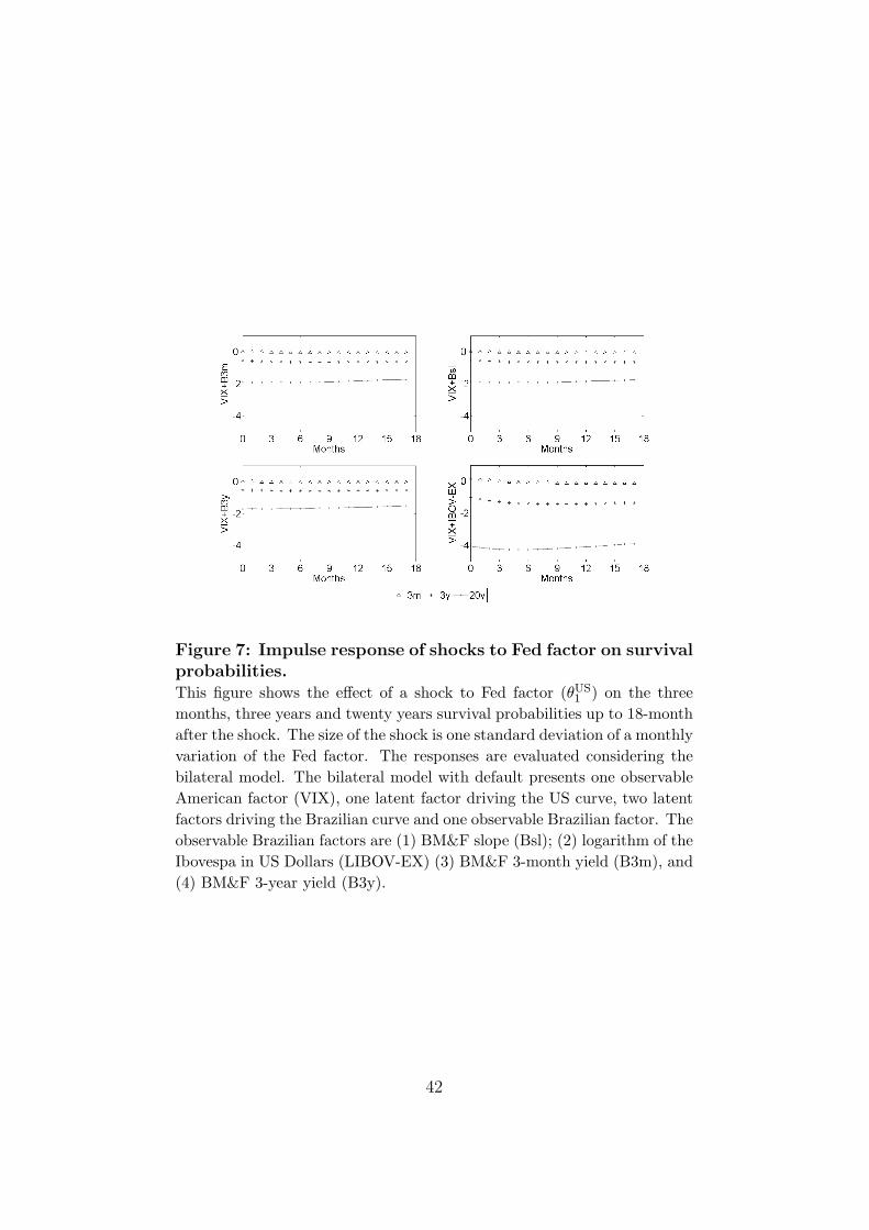
Figure 7: Impulse response of shocks to Fed factor on survivalprobabilities.This figure shows the effect of a shock to Fed factor (θUS
1 ) on the threemonths, three years and twenty years survival probabilities up to 18-monthafter the shock. The size of the shock is one standard deviation of a monthlyvariation of the Fed factor. The responses are evaluated considering thebilateral model. The bilateral model with default presents one observableAmerican factor (VIX), one latent factor driving the US curve, two latentfactors driving the Brazilian curve and one observable Brazilian factor. Theobservable Brazilian factors are (1) BM&F slope (Bsl); (2) logarithm of theIbovespa in US Dollars (LIBOV-EX) (3) BM&F 3-month yield (B3m), and(4) BM&F 3-year yield (B3y).
42
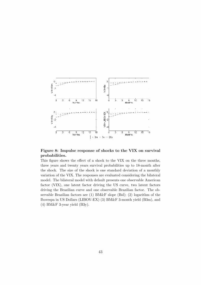
Figure 8: Impulse response of shocks to the VIX on survivalprobabilities.This figure shows the effect of a shock to the VIX on the three months,three years and twenty years survival probabilities up to 18-month afterthe shock. The size of the shock is one standard deviation of a monthlyvariation of the VIX. The responses are evaluated considering the bilateralmodel. The bilateral model with default presents one observable Americanfactor (VIX), one latent factor driving the US curve, two latent factorsdriving the Brazilian curve and one observable Brazilian factor. The ob-servable Brazilian factors are (1) BM&F slope (Bsl); (2) logarithm of theIbovespa in US Dollars (LIBOV-EX) (3) BM&F 3-month yield (B3m), and(4) BM&F 3-year yield (B3y).
43

Figure 9: Impulse response of shocks to observable Brazilianfactors on survival probabilities.This figure shows the effect of a shock to observable Brazilian factors onthe three months, three years and twenty years survival probabilities up to18-month after the shock. The size of the shock is one standard deviation ofa monthly variation of the observable factor. The responses are evaluatedconsidering the bilateral model. The bilateral model with default presentsone observable American factor (VIX), one latent factor driving the UScurve, two latent factors driving the Brazilian curve and one observableBrazilian factor. The observable Brazilian factors are (1) BM&F slope(Bsl); (2) logarithm of the Ibovespa in US Dollars (LIBOV-EX) (3) BM&F3-month yield (B3m), and (4) BM&F 3-year yield (B3y).
44

45
Banco Central do Brasil
Trabalhos para Discussão Os Trabalhos para Discussão podem ser acessados na internet, no formato PDF,
no endereço: http://www.bc.gov.br
Working Paper Series
Working Papers in PDF format can be downloaded from: http://www.bc.gov.br
1 Implementing Inflation Targeting in Brazil
Joel Bogdanski, Alexandre Antonio Tombini and Sérgio Ribeiro da Costa Werlang
Jul/2000
2 Política Monetária e Supervisão do Sistema Financeiro Nacional no Banco Central do Brasil Eduardo Lundberg Monetary Policy and Banking Supervision Functions on the Central Bank Eduardo Lundberg
Jul/2000
Jul/2000
3 Private Sector Participation: a Theoretical Justification of the Brazilian Position Sérgio Ribeiro da Costa Werlang
Jul/2000
4 An Information Theory Approach to the Aggregation of Log-Linear Models Pedro H. Albuquerque
Jul/2000
5 The Pass-Through from Depreciation to Inflation: a Panel Study Ilan Goldfajn and Sérgio Ribeiro da Costa Werlang
Jul/2000
6 Optimal Interest Rate Rules in Inflation Targeting Frameworks José Alvaro Rodrigues Neto, Fabio Araújo and Marta Baltar J. Moreira
Jul/2000
7 Leading Indicators of Inflation for Brazil Marcelle Chauvet
Sep/2000
8 The Correlation Matrix of the Brazilian Central Bank’s Standard Model for Interest Rate Market Risk José Alvaro Rodrigues Neto
Sep/2000
9 Estimating Exchange Market Pressure and Intervention Activity Emanuel-Werner Kohlscheen
Nov/2000
10 Análise do Financiamento Externo a uma Pequena Economia Aplicação da Teoria do Prêmio Monetário ao Caso Brasileiro: 1991–1998 Carlos Hamilton Vasconcelos Araújo e Renato Galvão Flôres Júnior
Mar/2001
11 A Note on the Efficient Estimation of Inflation in Brazil Michael F. Bryan and Stephen G. Cecchetti
Mar/2001
12 A Test of Competition in Brazilian Banking Márcio I. Nakane
Mar/2001

46
13 Modelos de Previsão de Insolvência Bancária no Brasil Marcio Magalhães Janot
Mar/2001
14 Evaluating Core Inflation Measures for Brazil Francisco Marcos Rodrigues Figueiredo
Mar/2001
15 Is It Worth Tracking Dollar/Real Implied Volatility? Sandro Canesso de Andrade and Benjamin Miranda Tabak
Mar/2001
16 Avaliação das Projeções do Modelo Estrutural do Banco Central do Brasil para a Taxa de Variação do IPCA Sergio Afonso Lago Alves Evaluation of the Central Bank of Brazil Structural Model’s Inflation Forecasts in an Inflation Targeting Framework Sergio Afonso Lago Alves
Mar/2001
Jul/2001
17 Estimando o Produto Potencial Brasileiro: uma Abordagem de Função de Produção Tito Nícias Teixeira da Silva Filho Estimating Brazilian Potential Output: a Production Function Approach Tito Nícias Teixeira da Silva Filho
Abr/2001
Aug/2002
18 A Simple Model for Inflation Targeting in Brazil Paulo Springer de Freitas and Marcelo Kfoury Muinhos
Apr/2001
19 Uncovered Interest Parity with Fundamentals: a Brazilian Exchange Rate Forecast Model Marcelo Kfoury Muinhos, Paulo Springer de Freitas and Fabio Araújo
May/2001
20 Credit Channel without the LM Curve Victorio Y. T. Chu and Márcio I. Nakane
May/2001
21 Os Impactos Econômicos da CPMF: Teoria e Evidência Pedro H. Albuquerque
Jun/2001
22 Decentralized Portfolio Management Paulo Coutinho and Benjamin Miranda Tabak
Jun/2001
23 Os Efeitos da CPMF sobre a Intermediação Financeira Sérgio Mikio Koyama e Márcio I. Nakane
Jul/2001
24 Inflation Targeting in Brazil: Shocks, Backward-Looking Prices, and IMF Conditionality Joel Bogdanski, Paulo Springer de Freitas, Ilan Goldfajn and Alexandre Antonio Tombini
Aug/2001
25 Inflation Targeting in Brazil: Reviewing Two Years of Monetary Policy 1999/00 Pedro Fachada
Aug/2001
26 Inflation Targeting in an Open Financially Integrated Emerging Economy: the Case of Brazil Marcelo Kfoury Muinhos
Aug/2001
27
Complementaridade e Fungibilidade dos Fluxos de Capitais Internacionais Carlos Hamilton Vasconcelos Araújo e Renato Galvão Flôres Júnior
Set/2001

47
28
Regras Monetárias e Dinâmica Macroeconômica no Brasil: uma Abordagem de Expectativas Racionais Marco Antonio Bonomo e Ricardo D. Brito
Nov/2001
29 Using a Money Demand Model to Evaluate Monetary Policies in Brazil Pedro H. Albuquerque and Solange Gouvêa
Nov/2001
30 Testing the Expectations Hypothesis in the Brazilian Term Structure of Interest Rates Benjamin Miranda Tabak and Sandro Canesso de Andrade
Nov/2001
31 Algumas Considerações sobre a Sazonalidade no IPCA Francisco Marcos R. Figueiredo e Roberta Blass Staub
Nov/2001
32 Crises Cambiais e Ataques Especulativos no Brasil Mauro Costa Miranda
Nov/2001
33 Monetary Policy and Inflation in Brazil (1975-2000): a VAR Estimation André Minella
Nov/2001
34 Constrained Discretion and Collective Action Problems: Reflections on the Resolution of International Financial Crises Arminio Fraga and Daniel Luiz Gleizer
Nov/2001
35 Uma Definição Operacional de Estabilidade de Preços Tito Nícias Teixeira da Silva Filho
Dez/2001
36 Can Emerging Markets Float? Should They Inflation Target? Barry Eichengreen
Feb/2002
37 Monetary Policy in Brazil: Remarks on the Inflation Targeting Regime, Public Debt Management and Open Market Operations Luiz Fernando Figueiredo, Pedro Fachada and Sérgio Goldenstein
Mar/2002
38 Volatilidade Implícita e Antecipação de Eventos de Stress: um Teste para o Mercado Brasileiro Frederico Pechir Gomes
Mar/2002
39 Opções sobre Dólar Comercial e Expectativas a Respeito do Comportamento da Taxa de Câmbio Paulo Castor de Castro
Mar/2002
40 Speculative Attacks on Debts, Dollarization and Optimum Currency Areas Aloisio Araujo and Márcia Leon
Apr/2002
41 Mudanças de Regime no Câmbio Brasileiro Carlos Hamilton V. Araújo e Getúlio B. da Silveira Filho
Jun/2002
42 Modelo Estrutural com Setor Externo: Endogenização do Prêmio de Risco e do Câmbio Marcelo Kfoury Muinhos, Sérgio Afonso Lago Alves e Gil Riella
Jun/2002
43 The Effects of the Brazilian ADRs Program on Domestic Market Efficiency Benjamin Miranda Tabak and Eduardo José Araújo Lima
Jun/2002

48
44 Estrutura Competitiva, Produtividade Industrial e Liberação Comercial no Brasil Pedro Cavalcanti Ferreira e Osmani Teixeira de Carvalho Guillén
Jun/2002
45 Optimal Monetary Policy, Gains from Commitment, and Inflation Persistence André Minella
Aug/2002
46 The Determinants of Bank Interest Spread in Brazil Tarsila Segalla Afanasieff, Priscilla Maria Villa Lhacer and Márcio I. Nakane
Aug/2002
47 Indicadores Derivados de Agregados Monetários Fernando de Aquino Fonseca Neto e José Albuquerque Júnior
Set/2002
48 Should Government Smooth Exchange Rate Risk? Ilan Goldfajn and Marcos Antonio Silveira
Sep/2002
49 Desenvolvimento do Sistema Financeiro e Crescimento Econômico no Brasil: Evidências de Causalidade Orlando Carneiro de Matos
Set/2002
50 Macroeconomic Coordination and Inflation Targeting in a Two-Country Model Eui Jung Chang, Marcelo Kfoury Muinhos and Joanílio Rodolpho Teixeira
Sep/2002
51 Credit Channel with Sovereign Credit Risk: an Empirical Test Victorio Yi Tson Chu
Sep/2002
52 Generalized Hyperbolic Distributions and Brazilian Data José Fajardo and Aquiles Farias
Sep/2002
53 Inflation Targeting in Brazil: Lessons and Challenges André Minella, Paulo Springer de Freitas, Ilan Goldfajn and Marcelo Kfoury Muinhos
Nov/2002
54 Stock Returns and Volatility Benjamin Miranda Tabak and Solange Maria Guerra
Nov/2002
55 Componentes de Curto e Longo Prazo das Taxas de Juros no Brasil Carlos Hamilton Vasconcelos Araújo e Osmani Teixeira de Carvalho de Guillén
Nov/2002
56 Causality and Cointegration in Stock Markets: the Case of Latin America Benjamin Miranda Tabak and Eduardo José Araújo Lima
Dec/2002
57 As Leis de Falência: uma Abordagem Econômica Aloisio Araujo
Dez/2002
58 The Random Walk Hypothesis and the Behavior of Foreign Capital Portfolio Flows: the Brazilian Stock Market Case Benjamin Miranda Tabak
Dec/2002
59 Os Preços Administrados e a Inflação no Brasil Francisco Marcos R. Figueiredo e Thaís Porto Ferreira
Dez/2002
60 Delegated Portfolio Management Paulo Coutinho and Benjamin Miranda Tabak
Dec/2002
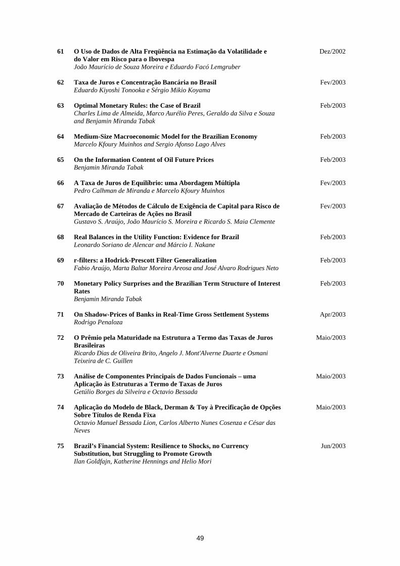
49
61 O Uso de Dados de Alta Freqüência na Estimação da Volatilidade e do Valor em Risco para o Ibovespa João Maurício de Souza Moreira e Eduardo Facó Lemgruber
Dez/2002
62 Taxa de Juros e Concentração Bancária no Brasil Eduardo Kiyoshi Tonooka e Sérgio Mikio Koyama
Fev/2003
63 Optimal Monetary Rules: the Case of Brazil Charles Lima de Almeida, Marco Aurélio Peres, Geraldo da Silva e Souza and Benjamin Miranda Tabak
Feb/2003
64 Medium-Size Macroeconomic Model for the Brazilian Economy Marcelo Kfoury Muinhos and Sergio Afonso Lago Alves
Feb/2003
65 On the Information Content of Oil Future Prices Benjamin Miranda Tabak
Feb/2003
66 A Taxa de Juros de Equilíbrio: uma Abordagem Múltipla Pedro Calhman de Miranda e Marcelo Kfoury Muinhos
Fev/2003
67 Avaliação de Métodos de Cálculo de Exigência de Capital para Risco de Mercado de Carteiras de Ações no Brasil Gustavo S. Araújo, João Maurício S. Moreira e Ricardo S. Maia Clemente
Fev/2003
68 Real Balances in the Utility Function: Evidence for Brazil Leonardo Soriano de Alencar and Márcio I. Nakane
Feb/2003
69 r-filters: a Hodrick-Prescott Filter Generalization Fabio Araújo, Marta Baltar Moreira Areosa and José Alvaro Rodrigues Neto
Feb/2003
70 Monetary Policy Surprises and the Brazilian Term Structure of Interest Rates Benjamin Miranda Tabak
Feb/2003
71 On Shadow-Prices of Banks in Real-Time Gross Settlement Systems Rodrigo Penaloza
Apr/2003
72 O Prêmio pela Maturidade na Estrutura a Termo das Taxas de Juros Brasileiras Ricardo Dias de Oliveira Brito, Angelo J. Mont'Alverne Duarte e Osmani Teixeira de C. Guillen
Maio/2003
73 Análise de Componentes Principais de Dados Funcionais – uma Aplicação às Estruturas a Termo de Taxas de Juros Getúlio Borges da Silveira e Octavio Bessada
Maio/2003
74 Aplicação do Modelo de Black, Derman & Toy à Precificação de Opções Sobre Títulos de Renda Fixa
Octavio Manuel Bessada Lion, Carlos Alberto Nunes Cosenza e César das Neves
Maio/2003
75 Brazil’s Financial System: Resilience to Shocks, no Currency Substitution, but Struggling to Promote Growth Ilan Goldfajn, Katherine Hennings and Helio Mori
Jun/2003

50
76 Inflation Targeting in Emerging Market Economies Arminio Fraga, Ilan Goldfajn and André Minella
Jun/2003
77 Inflation Targeting in Brazil: Constructing Credibility under Exchange Rate Volatility André Minella, Paulo Springer de Freitas, Ilan Goldfajn and Marcelo Kfoury Muinhos
Jul/2003
78 Contornando os Pressupostos de Black & Scholes: Aplicação do Modelo de Precificação de Opções de Duan no Mercado Brasileiro Gustavo Silva Araújo, Claudio Henrique da Silveira Barbedo, Antonio Carlos Figueiredo, Eduardo Facó Lemgruber
Out/2003
79 Inclusão do Decaimento Temporal na Metodologia Delta-Gama para o Cálculo do VaR de Carteiras Compradas em Opções no Brasil Claudio Henrique da Silveira Barbedo, Gustavo Silva Araújo, Eduardo Facó Lemgruber
Out/2003
80 Diferenças e Semelhanças entre Países da América Latina: uma Análise de Markov Switching para os Ciclos Econômicos de Brasil e Argentina Arnildo da Silva Correa
Out/2003
81 Bank Competition, Agency Costs and the Performance of the Monetary Policy Leonardo Soriano de Alencar and Márcio I. Nakane
Jan/2004
82 Carteiras de Opções: Avaliação de Metodologias de Exigência de Capital no Mercado Brasileiro Cláudio Henrique da Silveira Barbedo e Gustavo Silva Araújo
Mar/2004
83 Does Inflation Targeting Reduce Inflation? An Analysis for the OECD Industrial Countries Thomas Y. Wu
May/2004
84 Speculative Attacks on Debts and Optimum Currency Area: a Welfare Analysis Aloisio Araujo and Marcia Leon
May/2004
85 Risk Premia for Emerging Markets Bonds: Evidence from Brazilian Government Debt, 1996-2002 André Soares Loureiro and Fernando de Holanda Barbosa
May/2004
86 Identificação do Fator Estocástico de Descontos e Algumas Implicações sobre Testes de Modelos de Consumo Fabio Araujo e João Victor Issler
Maio/2004
87 Mercado de Crédito: uma Análise Econométrica dos Volumes de Crédito Total e Habitacional no Brasil Ana Carla Abrão Costa
Dez/2004
88 Ciclos Internacionais de Negócios: uma Análise de Mudança de Regime Markoviano para Brasil, Argentina e Estados Unidos Arnildo da Silva Correa e Ronald Otto Hillbrecht
Dez/2004
89 O Mercado de Hedge Cambial no Brasil: Reação das Instituições Financeiras a Intervenções do Banco Central Fernando N. de Oliveira
Dez/2004
51
90 Bank Privatization and Productivity: Evidence for Brazil Márcio I. Nakane and Daniela B. Weintraub
Dec/2004
91 Credit Risk Measurement and the Regulation of Bank Capital and Provision Requirements in Brazil – a Corporate Analysis Ricardo Schechtman, Valéria Salomão Garcia, Sergio Mikio Koyama and Guilherme Cronemberger Parente
Dec/2004
92
Steady-State Analysis of an Open Economy General Equilibrium Model for Brazil Mirta Noemi Sataka Bugarin, Roberto de Goes Ellery Jr., Victor Gomes Silva, Marcelo Kfoury Muinhos
Apr/2005
93 Avaliação de Modelos de Cálculo de Exigência de Capital para Risco Cambial Claudio H. da S. Barbedo, Gustavo S. Araújo, João Maurício S. Moreira e Ricardo S. Maia Clemente
Abr/2005
94 Simulação Histórica Filtrada: Incorporação da Volatilidade ao Modelo Histórico de Cálculo de Risco para Ativos Não-Lineares Claudio Henrique da Silveira Barbedo, Gustavo Silva Araújo e Eduardo Facó Lemgruber
Abr/2005
95 Comment on Market Discipline and Monetary Policy by Carl Walsh Maurício S. Bugarin and Fábia A. de Carvalho
Apr/2005
96 O que É Estratégia: uma Abordagem Multiparadigmática para a Disciplina Anthero de Moraes Meirelles
Ago/2005
97 Finance and the Business Cycle: a Kalman Filter Approach with Markov Switching Ryan A. Compton and Jose Ricardo da Costa e Silva
Aug/2005
98 Capital Flows Cycle: Stylized Facts and Empirical Evidences for Emerging Market Economies Helio Mori e Marcelo Kfoury Muinhos
Aug/2005
99 Adequação das Medidas de Valor em Risco na Formulação da Exigência de Capital para Estratégias de Opções no Mercado Brasileiro Gustavo Silva Araújo, Claudio Henrique da Silveira Barbedo,e Eduardo Facó Lemgruber
Set/2005
100 Targets and Inflation Dynamics Sergio A. L. Alves and Waldyr D. Areosa
Oct/2005
101 Comparing Equilibrium Real Interest Rates: Different Approaches to Measure Brazilian Rates Marcelo Kfoury Muinhos and Márcio I. Nakane
Mar/2006
102 Judicial Risk and Credit Market Performance: Micro Evidence from Brazilian Payroll Loans Ana Carla A. Costa and João M. P. de Mello
Apr/2006
103 The Effect of Adverse Supply Shocks on Monetary Policy and Output Maria da Glória D. S. Araújo, Mirta Bugarin, Marcelo Kfoury Muinhos and Jose Ricardo C. Silva
Apr/2006
52
104 Extração de Informação de Opções Cambiais no Brasil Eui Jung Chang e Benjamin Miranda Tabak
Abr/2006
105 Representing Roommate’s Preferences with Symmetric Utilities José Alvaro Rodrigues Neto
Apr/2006
106 Testing Nonlinearities Between Brazilian Exchange Rates and Inflation Volatilities Cristiane R. Albuquerque and Marcelo Portugal
May/2006
107 Demand for Bank Services and Market Power in Brazilian Banking Márcio I. Nakane, Leonardo S. Alencar and Fabio Kanczuk
Jun/2006
108 O Efeito da Consignação em Folha nas Taxas de Juros dos Empréstimos Pessoais Eduardo A. S. Rodrigues, Victorio Chu, Leonardo S. Alencar e Tony Takeda
Jun/2006
109 The Recent Brazilian Disinflation Process and Costs Alexandre A. Tombini and Sergio A. Lago Alves
Jun/2006
110 Fatores de Risco e o Spread Bancário no Brasil Fernando G. Bignotto e Eduardo Augusto de Souza Rodrigues
Jul/2006
111 Avaliação de Modelos de Exigência de Capital para Risco de Mercado do Cupom Cambial Alan Cosme Rodrigues da Silva, João Maurício de Souza Moreira e Myrian Beatriz Eiras das Neves
Jul/2006
112 Interdependence and Contagion: an Analysis of Information Transmission in Latin America's Stock Markets Angelo Marsiglia Fasolo
Jul/2006
113 Investigação da Memória de Longo Prazo da Taxa de Câmbio no Brasil Sergio Rubens Stancato de Souza, Benjamin Miranda Tabak e Daniel O. Cajueiro
Ago/2006
114 The Inequality Channel of Monetary Transmission Marta Areosa and Waldyr Areosa
Aug/2006
115 Myopic Loss Aversion and House-Money Effect Overseas: an Experimental Approach José L. B. Fernandes, Juan Ignacio Peña and Benjamin M. Tabak
Sep/2006
116 Out-Of-The-Money Monte Carlo Simulation Option Pricing: the Join Use of Importance Sampling and Descriptive Sampling Jaqueline Terra Moura Marins, Eduardo Saliby and Joséte Florencio dos Santos
Sep/2006
117 An Analysis of Off-Site Supervision of Banks’ Profitability, Risk and Capital Adequacy: a Portfolio Simulation Approach Applied to Brazilian Banks Theodore M. Barnhill, Marcos R. Souto and Benjamin M. Tabak
Sep/2006
118 Contagion, Bankruptcy and Social Welfare Analysis in a Financial Economy with Risk Regulation Constraint Aloísio P. Araújo and José Valentim M. Vicente
Oct/2006

53
119 A Central de Risco de Crédito no Brasil: uma Análise de Utilidade de Informação Ricardo Schechtman
Out/2006
120 Forecasting Interest Rates: an Application for Brazil Eduardo J. A. Lima, Felipe Luduvice and Benjamin M. Tabak
Oct/2006
121 The Role of Consumer’s Risk Aversion on Price Rigidity Sergio A. Lago Alves and Mirta N. S. Bugarin
Nov/2006
122 Nonlinear Mechanisms of the Exchange Rate Pass-Through: a Phillips Curve Model With Threshold for Brazil Arnildo da Silva Correa and André Minella
Nov/2006
123 A Neoclassical Analysis of the Brazilian “Lost-Decades” Flávia Mourão Graminho
Nov/2006
124 The Dynamic Relations between Stock Prices and Exchange Rates: Evidence for Brazil Benjamin M. Tabak
Nov/2006
125 Herding Behavior by Equity Foreign Investors on Emerging Markets Barbara Alemanni and José Renato Haas Ornelas
Dec/2006
126 Risk Premium: Insights over the Threshold José L. B. Fernandes, Augusto Hasman and Juan Ignacio Peña
Dec/2006
127 Uma Investigação Baseada em Reamostragem sobre Requerimentos de Capital para Risco de Crédito no Brasil Ricardo Schechtman
Dec/2006
128 Term Structure Movements Implicit in Option Prices Caio Ibsen R. Almeida and José Valentim M. Vicente
Dec/2006
129 Brazil: Taming Inflation Expectations Afonso S. Bevilaqua, Mário Mesquita and André Minella
Jan/2007
130 The Role of Banks in the Brazilian Interbank Market: Does Bank Type Matter? Daniel O. Cajueiro and Benjamin M. Tabak
Jan/2007
131 Long-Range Dependence in Exchange Rates: the Case of the European Monetary System Sergio Rubens Stancato de Souza, Benjamin M. Tabak and Daniel O. Cajueiro
Mar/2007
132 Credit Risk Monte Carlo Simulation Using Simplified Creditmetrics’ Model: the Joint Use of Importance Sampling and Descriptive Sampling Jaqueline Terra Moura Marins and Eduardo Saliby
Mar/2007
133 A New Proposal for Collection and Generation of Information on Financial Institutions’ Risk: the Case of Derivatives Gilneu F. A. Vivan and Benjamin M. Tabak
Mar/2007
134 Amostragem Descritiva no Apreçamento de Opções Européias através de Simulação Monte Carlo: o Efeito da Dimensionalidade e da Probabilidade de Exercício no Ganho de Precisão Eduardo Saliby, Sergio Luiz Medeiros Proença de Gouvêa e Jaqueline Terra Moura Marins
Abr/2007

54
135 Evaluation of Default Risk for the Brazilian Banking Sector Marcelo Y. Takami and Benjamin M. Tabak
May/2007
136 Identifying Volatility Risk Premium from Fixed Income Asian Options Caio Ibsen R. Almeida and José Valentim M. Vicente
May/2007
137 Monetary Policy Design under Competing Models of Inflation Persistence Solange Gouvea e Abhijit Sen Gupta
May/2007
138 Forecasting Exchange Rate Density Using Parametric Models: the Case of Brazil Marcos M. Abe, Eui J. Chang and Benjamin M. Tabak
May/2007
139 Selection of Optimal Lag Length inCointegrated VAR Models with Weak Form of Common Cyclical Features Carlos Enrique Carrasco Gutiérrez, Reinaldo Castro Souza and Osmani Teixeira de Carvalho Guillén
Jun/2007
140 Inflation Targeting, Credibility and Confidence Crises Rafael Santos and Aloísio Araújo
Aug/2007
141 Forecasting Bonds Yields in the Brazilian Fixed income Market Jose Vicente and Benjamin M. Tabak
Aug/2007
142 Crises Análise da Coerência de Medidas de Risco no Mercado Brasileiro de Ações e Desenvolvimento de uma Metodologia Híbrida para o Expected Shortfall Alan Cosme Rodrigues da Silva, Eduardo Facó Lemgruber, José Alberto Rebello Baranowski e Renato da Silva Carvalho
Ago/2007
143 Price Rigidity in Brazil: Evidence from CPI Micro Data Solange Gouvea
Sep/2007
144 The Effect of Bid-Ask Prices on Brazilian Options Implied Volatility: a Case Study of Telemar Call Options Claudio Henrique da Silveira Barbedo and Eduardo Facó Lemgruber
Oct/2007
145 The Stability-Concentration Relationship in the Brazilian Banking System Benjamin Miranda Tabak, Solange Maria Guerra, Eduardo José Araújo Lima and Eui Jung Chang
Oct/2007
146 Movimentos da Estrutura a Termo e Critérios de Minimização do Erro de Previsão em um Modelo Paramétrico Exponencial Caio Almeida, Romeu Gomes, André Leite e José Vicente
Out/2007
147 Explaining Bank Failures in Brazil: Micro, Macro and Contagion Effects (1994-1998) Adriana Soares Sales and Maria Eduarda Tannuri-Pianto
Oct/2007
148 Um Modelo de Fatores Latentes com Variáveis Macroeconômicas para a Curva de Cupom Cambial Felipe Pinheiro, Caio Almeida e José Vicente
Out/2007
149 Joint Validation of Credit Rating PDs under Default Correlation Ricardo Schechtman
Oct/2007
55
150 A Probabilistic Approach for Assessing the Significance of Contextual Variables in Nonparametric Frontier Models: an Application for Brazilian Banks Roberta Blass Staub and Geraldo da Silva e Souza
Oct/2007
151 Building Confidence Intervals with Block Bootstraps for the Variance Ratio Test of Predictability
Nov/2007
Eduardo José Araújo Lima and Benjamin Miranda Tabak
152 Demand for Foreign Exchange Derivatives in Brazil: Hedge or Speculation? Fernando N. de Oliveira and Walter Novaes
Dec/2007
153 Aplicação da Amostragem por Importância à Simulação de Opções Asiáticas Fora do Dinheiro Jaqueline Terra Moura Marins
Dez/2007
154 Identification of Monetary Policy Shocks in the Brazilian Market for Bank Reserves Adriana Soares Sales and Maria Tannuri-Pianto
Dec/2007
155 Does Curvature Enhance Forecasting? Caio Almeida, Romeu Gomes, André Leite and José Vicente
Dec/2007
156 Escolha do Banco e Demanda por Empréstimos: um Modelo de Decisão em Duas Etapas Aplicado para o Brasil Sérgio Mikio Koyama e Márcio I. Nakane
Dez/2007
157 Is the Investment-Uncertainty Link Really Elusive? The Harmful Effects of Inflation Uncertainty in Brazil Tito Nícias Teixeira da Silva Filho
Jan/2008
158 Characterizing the Brazilian Term Structure of Interest Rates Osmani T. Guillen and Benjamin M. Tabak
Feb/2008
159 Behavior and Effects of Equity Foreign Investors on Emerging Markets Barbara Alemanni and José Renato Haas Ornelas
Feb/2008
160 The Incidence of Reserve Requirements in Brazil: Do Bank Stockholders Share the Burden? Fábia A. de Carvalho and Cyntia F. Azevedo
Feb/2008
161 Evaluating Value-at-Risk Models via Quantile Regressions Wagner P. Gaglianone, Luiz Renato Lima and Oliver Linton
Feb/2008
162 Balance Sheet Effects in Currency Crises: Evidence from Brazil Marcio M. Janot, Márcio G. P. Garcia and Walter Novaes
Apr/2008
163 Searching for the Natural Rate of Unemployment in a Large Relative Price Shocks’ Economy: the Brazilian Case Tito Nícias Teixeira da Silva Filho
May/2008
164 Foreign Banks’ Entry and Departure: the recent Brazilian experience (1996-2006) Pedro Fachada
Jun/2008
165 Avaliação de Opções de Troca e Opções de Spread Européias e Americanas Giuliano Carrozza Uzêda Iorio de Souza, Carlos Patrício Samanez e Gustavo Santos Raposo
Jul/2008
56
166 Testing Hyperinflation Theories Using the Inflation Tax Curve: a case study Fernando de Holanda Barbosa and Tito Nícias Teixeira da Silva Filho
Jul/2008
167 O Poder Discriminante das Operações de Crédito das Instituições Financeiras Brasileiras Clodoaldo Aparecido Annibal
Jul/2008
168 An Integrated Model for Liquidity Management and Short-Term Asset Allocation in Commercial Banks Wenersamy Ramos de Alcântara
Jul/2008
169 Mensuração do Risco Sistêmico no Setor Bancário com Variáveis Contábeis e Econômicas Lucio Rodrigues Capelletto, Eliseu Martins e Luiz João Corrar
Jul/2008
170 Política de Fechamento de Bancos com Regulador Não-Benevolente: Resumo e Aplicação Adriana Soares Sales
Jul/2008
171 Modelos para a Utilização das Operações de Redesconto pelos Bancos com Carteira Comercial no Brasil Sérgio Mikio Koyama e Márcio Issao Nakane
Ago/2008
172 Combining Hodrick-Prescott Filtering with a Production Function Approach to Estimate Output Gap Marta Areosa
Aug/2008
173 Exchange Rate Dynamics and the Relationship between the Random Walk Hypothesis and Official Interventions Eduardo José Araújo Lima and Benjamin Miranda Tabak
Aug/2008
174 Foreign Exchange Market Volatility Information: an investigation of real-dollar exchange rate Frederico Pechir Gomes, Marcelo Yoshio Takami and Vinicius Ratton Brandi
Aug/2008
175 Evaluating Asset Pricing Models in a Fama-French Framework Carlos Enrique Carrasco Gutierrez and Wagner Piazza Gaglianone
Dec/2008
176 Fiat Money and the Value of Binding Portfolio Constraints Mário R. Páscoa, Myrian Petrassi and Juan Pablo Torres-Martínez
Dec/2008
177 Preference for Flexibility and Bayesian Updating Gil Riella
Dec/2008
178 An Econometric Contribution to the Intertemporal Approach of the Current Account Wagner Piazza Gaglianone and João Victor Issler
Dec/2008
179 Are Interest Rate Options Important for the Assessment of Interest Rate Risk? Caio Almeida and José Vicente
Dec/2008
180 A Class of Incomplete and Ambiguity Averse Preferences Leandro Nascimento and Gil Riella
Dec/2008
181 Monetary Channels in Brazil through the Lens of a Semi-Structural Model André Minella and Nelson F. Souza-Sobrinho
Apr/2009

57
182 Avaliação de Opções Americanas com Barreiras Monitoradas de Forma Discreta Giuliano Carrozza Uzêda Iorio de Souza e Carlos Patrício Samanez
Abr/2009
183 Ganhos da Globalização do Capital Acionário em Crises Cambiais Marcio Janot e Walter Novaes
Abr/2009
184 Behavior Finance and Estimation Risk in Stochastic Portfolio Optimization José Luiz Barros Fernandes, Juan Ignacio Peña and Benjamin Miranda Tabak
Apr/2009
185 Market Forecasts in Brazil: performance and determinants Fabia A. de Carvalho and André Minella
Apr/2009
186 Previsão da Curva de Juros: um modelo estatístico com variáveis macroeconômicas André Luís Leite, Romeu Braz Pereira Gomes Filho e José Valentim Machado Vicente
Maio/2009
187 The Influence of Collateral on Capital Requirements in the Brazilian Financial System: an approach through historical average and logistic regression on probability of default Alan Cosme Rodrigues da Silva, Antônio Carlos Magalhães da Silva, Jaqueline Terra Moura Marins, Myrian Beatriz Eiras da Neves and Giovani Antonio Silva Brito
Jun/2009
188 Pricing Asian Interest Rate Options with a Three-Factor HJM Model Claudio Henrique da Silveira Barbedo, José Valentim Machado Vicente and Octávio Manuel Bessada Lion
Jun/2009
189 Linking Financial and Macroeconomic Factors to Credit Risk Indicators of Brazilian Banks Marcos Souto, Benjamin M. Tabak and Francisco Vazquez
Jul/2009
190 Concentração Bancária, Lucratividade e Risco Sistêmico: uma abordagem de contágio indireto Bruno Silva Martins e Leonardo S. Alencar
Set/2009
191 Concentração e Inadimplência nas Carteiras de Empréstimos dos Bancos Brasileiros Patricia L. Tecles, Benjamin M. Tabak e Roberta B. Staub
Set/2009
192 Inadimplência do Setor Bancário Brasileiro: uma avaliação de suas medidas Clodoaldo Aparecido Annibal
Set/2009
193 Loss Given Default: um estudo sobre perdas em operações prefixadas no mercado brasileiro Antonio Carlos Magalhães da Silva, Jaqueline Terra Moura Marins e Myrian Beatriz Eiras das Neves
Set/2009
194 Testes de Contágio entre Sistemas Bancários – A crise do subprime Benjamin M. Tabak e Manuela M. de Souza
Set/2009
195 From Default Rates to Default Matrices: a complete measurement of Brazilian banks' consumer credit delinquency Ricardo Schechtman
Oct/2009


