The Role of the Hydraulic Jump Phenomenon in the Rapid Spread of the 8-9 October 2017 Tubbs Fire

A THESIS

SUBMITTED TO THE DEPARTMENT OF EARTH SCIENCES OF SAN FRANCISCO STATE UNIVERSITY

IN PARTIAL FULFILLMENT OF THE REQUIREMENTS FOR THE DEGREE OF BACHELOR OF SCIENCE

By Natalie Corkhill

November 27, 2018

Thesis Advisors:

I certify that I have read this thesis and find it fully adequate, in scope and quality, as a Senior

Thesis for Bachelor of Science.

_____________________________________________ John P. Monteverdi, Professor of Meteorology

I certify that I have read this thesis and find it fully adequate, in scope and quality, as a Senior

Thesis for Bachelor of Science.

______________________________________________ David P. Dempsey, Emeritus Professor of Meteorology

2

Abstract

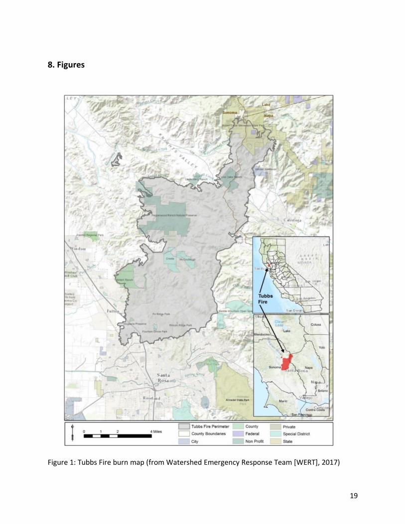
On the evening of October 8, 2017, a series of wildfires developed and spread over

nearly 250,000 acres in Napa and Sonoma Counties of Northern California (Fig. 1). The largest

of these started near Tubbs Lane in Calistoga, CA (named appropriately the “Tubbs Fire”) and

fanned by strong winds moved rapidly southwestward to devastate parts of Santa Rosa.

Analyses of synoptic, mesoscale, and thermodynamic conditions during the first 24 hours of the

Tubbs Fire indicate that the weather pattern corresponded to the quintessential “Diablo Wind

Pattern”, characterized by strong offshore flow over the northern San Francisco Bay Region.

The observed flow in the boundary layer was at right angles to terrain features in the

Mayacamas Mountains (with crests at roughly 800 m (2500 ft)) at the same time that actual

and objectively-produced model soundings showed a strong stable layer/temperature inversion

near the top of the range. These conditions met the criteria described in the literature for

enhanced downslope winds/hydraulic jump. In that case, the hypothesis presented here is that

ducted, augmented flow occurred over the ridge tops and down the southwestern slopes of the

mountains into the Coffey Park neighborhood of Santa Rosa. The Weather Research and

Forecasting (WRF-ARW) model was used with 1.1 km horizontal grid resolution to resolve

features of the flow (or wind) pattern forced by the Mayacamas Mountains and other

topographic features in the North Bay Area. The model produced realistic values of wind speeds

(when compared to actual observations) over the model domain. The results of the simulation

confirmed the hypothesis that the hydraulic jump phenomenon did occur for the conditions

that existed in the area on 8-9 October 2017.

3

1. Introduction

There has been much research on the synoptic-scale pattern associated with offshore

wind patterns in California (Monteverdi, 1973; McCutchan and Schroeder, 1973, and many

others). In the last fifteen years or so, these studies have concentrated not only on the synoptic

scale and mesoscale dynamics of these patterns, but also on the ability of forecasters and

forecasting models to predict them (Jones et. al., 2010). Most recently, there has been a

research focus on the local environmental impacts of the wildfires that develop in these

patterns and how such winds and fires interact with coastal topography of Southern California

(see, for e.g., Jones et. al., 2010).

Since 1990, research efforts also have been directed towards understanding the

strength of the winds that impact California coastal sections during these events. It has been

observed by weather forecasters that the strength of the sustained winds seems inconsistently

large given the surface synoptic-scale pressure gradients. Objective modeling of the key

thermodynamic and dynamics controls on these patterns (Gabersek and Durran, 2006) has

shown that both gap flow and the phenomenon known as the “hydraulic jump” explain much of

the mesoscale augmentation of the surface wind speed patterns on leeward hill slopes, and at

ridge top levels. All of this research centered on the issues associated with Santa Ana Winds

and there has been none in the formal literature about the wind patterns associated with

Diablo Winds.

The purpose of this research is to document the synoptic and mesoscale controls on the

development of the extreme winds associated with the Tubbs Fire of October 8-9, 2017 that

devastated portions of Santa Rosa California (Fig. 1). My hypothesis is that the synoptic and

4

mesoscale meteorological conditions present over north-central California suggested that during

the night and early morning of October 8 and 9, 2017 a well-developed hydraulic jump should be

present with a downslope augmentation of flow leeward of the western range of the Mayacamas

Mountains. To depict whether the hydraulic jump phenomenon did indeed occur that night,

high-resolution simulations of wind, potential temperature, and vertical velocity patterns will be

created using the Weather Research and Forecasting (WRF-ARW) model in a domain centered

on the Tubbs Fire area.

2. General Background

2.1 The Tubbs Fire of October 8-9, 2017

The Tubbs fire started around 9:43pm on October 8 and was not fully contained until

October 31, 2018. It is the second most destructive fire in California history to date 1, burning

36,807 acres of land and 5,636 structures, and killing 22 people (Cal Fire, 2018a). Although the

cause of the fire is still under investigation, there were multiple reports of downed power lines

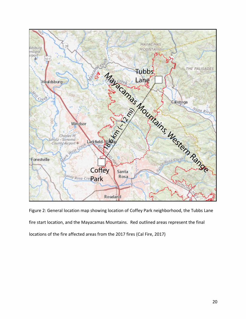
and exploding transformers in the North Bay region. One fire start occurred near Tubbs Lane in

the town of Calistoga (Fig. 2). Pushed by strong northeasterly winds known locally as ‘Diablo

Winds’, the front of this fire moved more than 19 km (12 miles) in its first three hours (CAL Fire,

2018b) as winds on the leeward (southwest) side of the Mayacamas Mountains increased to 18

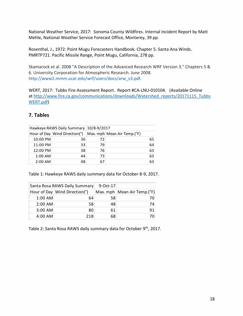
m s-1(40 mph) with gusts up to 35 m s-1 (78 mph) (Tables 1 and 2). Between 3 and 4am, winds

1 On November 8, 2018, a wildfire that began in Plumas National Forest in Northern California swept through the town of Paradise, California. At least killing 71 persons, destroying over 7000 structures, and covering 142,00 acres (221 mi2; 573 km2) (Cal Fire, 2018a).

5

were strong enough to loft burning debris across the six-lane Highway 101 freeway into the

Coffey Park neighborhood.

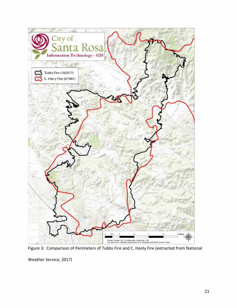
In 1964 the C. Hanly Fire burned nearly the same area as the Tubbs Fire (Fig. 3). This fire

was also fanned by strong northeasterly winds. The major difference between the two fires is

that the Hanly fire burned mostly undeveloped land. Since 1964, hundreds of houses and

businesses were built in the area. The fact that two large fires covering roughly the same areas

associated with strong offshore winds suggests that this region is susceptible for fires to spread

into.

2.2 Diablo Winds

The weather pattern associated with strong offshore flow in California often occurs in

the late summer and early fall and is called the Diablo Wind pattern in north-central California.

The term first appeared shortly after the 1991 Oakland Hills firestorm, perhaps to distinguish it

from the comparable, and more familiar, hot dry wind in Southern California known as

the Santa Ana Winds. In fact, in decades previous to the 1991 fire, the term "Santa Ana" was

occasionally used as well for the Bay Area dry northeasterly winds (Monteverdi, 1973;

Rosenthal, 1972).

Diablo Winds usually occur when there is a transitory surface high pressure area over

the Great Basin or Pacific Northwest and a low pressure area to the southeast. This pattern can

begin to occur in late summer to early fall when the polar jet stream begins its seasonal

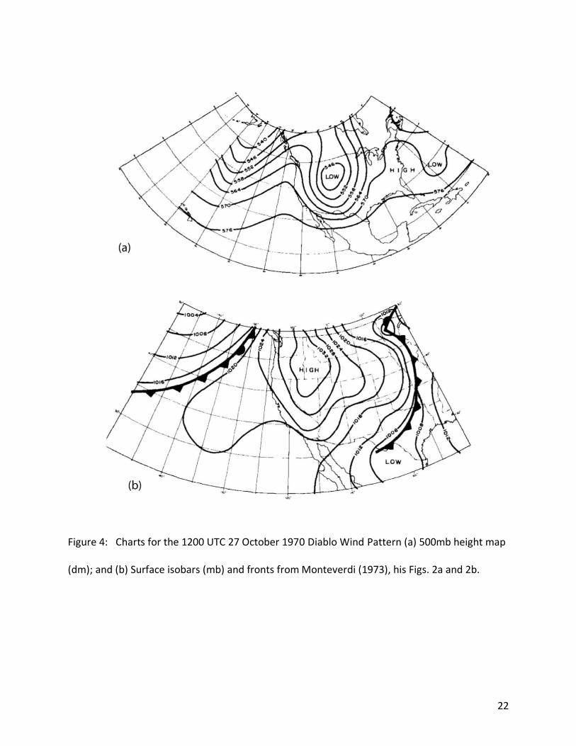
repositioning southward. As a trough in the middle and upper troposphere moves

southeastward into the southwest United States, it is followed by a ridge in the middle and

upper troposphere. An example is shown in Monteverdi (1973) for the Diablo wind event that

6

occurred on 27 October 1970 (Fig. 4a). This is the reverse of the normal summertime weather

pattern in which an area of low pressure (called the California Thermal Low) rather than high

pressure lies east of the Bay Area, drawing in cooler, more humid air from the ocean. Wind

convergence between these two features is associated with strong subsidence in the mid

troposphere and pressure rises at the surface leading to a surface anticyclone over that the

Pacific Northwest (Fig. 4b). Surface winds begin to flow outward from the surface high and

emerge over California as northeast winds.

Air moving from the Great Basin to the Pacific coast in late summer and early fall is hot

and dry for several reasons. Originating from the desert areas of the Great Basin, this air is hot

from being in contact with a relatively hot surface and is dry due to low water vapor content (as

measured by the dew point) and low relative humidity (as measured by large difference

between temperature and dew point). In addition, northeasterly winds moving from the Great

Basin subsides on the order of 1500 m (5000 ft). Such air adiabatically compresses and warms

at a rate of about 10°C km-1 (5.5°F 1000ft-1). The compressional warming of the air also

increases the difference between the dew point and temperature, further lowering the relative

humidity.

When offshore winds are forecast to be especially strong, hot, and dry, a Red Flag

Warning will be issued by the National Weather Service (NWS). A Red Flag Warning means that

critical fire weather conditions are occurring and that a combination of strong winds, low

relative humidity, and warm temperatures can contribute to extreme fire behavior. The

conditions leading to a Red Flag Warning are most dangerous during the late summer and fall in

California when vegetation is dried out and susceptible to fire.

7

An additional factor creates additional danger associated with Diablo Winds. When

these already strong wind encounter mountain ranges at right angles, flow tends to be

‘funnelled’ by mountain passes and canyons. In certain conditions, flow also can be

constrained by temperature structures located at tops of mountain ranges, favoring the

development of excessive wind speeds at the top of ridges and on the downwind (lee) slopes.

Thus, the already strong winds can be significantly augmented by the topography of north-

central California.

2.3 Downslope Windstorms

Since the 1980s, there has been an extensive literature on the conditions that precede

the development of what are now known as “downslope windstorms”. These are wind storms

that occur on the lee slope of mountain ranges. These events occur when strong winds

approach a mountain range under a stable layer that conceptually acts as a “lid”, constraining

the flow beneath. Durran (1990) showed that strong surface flow directed orthogonally against

a mountain barrier can produce locally strong wind storms on the leeward slope when certain

conditions are met: (a) strong winds at right angles to the topography; (b) an inversion at the

level of the top of the local mountains; and (c) an adequate combination of thermodynamic and

wind speed factors that ensure the wind will be constrained into a narrow layer of augmented

flow from the crest to the downslope side. These conditions are associated with a flow

configuration known as a “hydraulic jump” by engineers.

As early as 1964, meteorologists have recognized the flow patterns that can develop in

the atmosphere to produce a configuration resulting in an atmospheric hydraulic jump, in

which flow approaching a range is accelerated at ridge top and lee-side slope, and then ascends

8

in a massive turbulent wave (Lied, 1964). The tendency for this to occur in the atmosphere can

be estimated by factors that include the height of the mountain range orthogonal to the flow,

the strength of the orthogonal flow, and the stability of the layer that is just at or above the

mountain ridge.

This has been estimated in many studies by calculation of the Froude Number (Fr)

(Markowski and Richardson, 2010, p. 336), which is written as follows:

𝐹𝑟 =𝑈ℎ⁄

𝑁 (Equation 1)

where U is the wind speed normal to the mountain range, h is the height of the mountains, and

N is the Brunt–Väisälä frequency (related to the atmospheric stability).

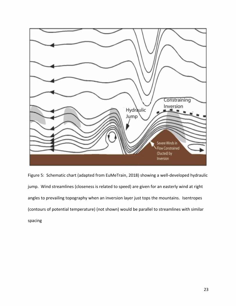
The Froude number can be used to estimate whether winds approaching a mountain

barrier at right angles will either be “ducted” into a narrow layer of accelerating air down the

leeward slope associated with the hydraulic jump phenomenon (Fig. 5) or move around/over the

mountain unobstructed. The Froude number must be approximately equal to 1 for the hydraulic

jump configuration to occur.

The author performed some calculations of the Froude number based upon the

difference in the elevation of the northern Napa Valley (where the ignition area of the fire is

thought to have been (see Fig. 2)) and the height of the Mayacamas Mountain range; this

difference is approximately 1100 m. The procedure used is examined in more detail in Section

3.2. Analyses of the actual sounding information from Oakland International Airport and the

estimated soundings from the North American Model (NAM) (discussed in Section 3.2) indicates

that an isothermal/stable layer was present near the top of the mountains. Wind speeds at the

ridge top obtained roughly from the sounding data indicate that wind speeds at ridge level were

9

20 m s-1. These conditions persisted for much of the late afternoon of 8 October 2017 to the early

morning.

Insertion of these values into Equation (1) showed that the Froude Number was near 1 at

the crest of the Mayacamas Mountains at the time. The author realizes that these are rough

estimates. Nevertheless, this suggests that flow could be constrained in a narrow layer only over

the top of this range and, if so, a well-developed mountain wave with accelerated downslope

flow and perhaps a hydraulic jump wave would have been present, with “ducting” from the crest

westward to the base of the leeward slope. Isentropes should be packed tightly in ducted flow,

with a “leap” of the isentropes just west of the leeward base of the flow. This hypothesis will be

tested in Section 4 below, in which numerical simulations of the two- and three-dimensional flow

patterns in the area will be estimated using the WRF model.

3. Synoptic and Mesoscale Meteorology of the Event

3.1 Synoptic-scale Controls On October 8, 2018, the synoptic pattern that was in place over north-central California

matched the Diablo Wind archetype discussed in Section 2.2. This pattern includes deep

subsidence in the middle troposphere related to convergence occurring at jet stream level in

the upper troposphere. This in turn is associated with surface high pressure area over the

Great Basin or Pacific Northwest. Because this Diablo Wind pattern was expected, on October

6, 2017 the National Weather Service issued Red Flag Warnings for extreme fire weather

conditions over the area covering the period 11AM October 8 to 5AM October 9, 2017 (NWS,

2017).

10

During the period from October 7 to 10, 2017, a high amplitude short wave trough

passed across the Pacific Northwest and move southeastward into the Southwestern United

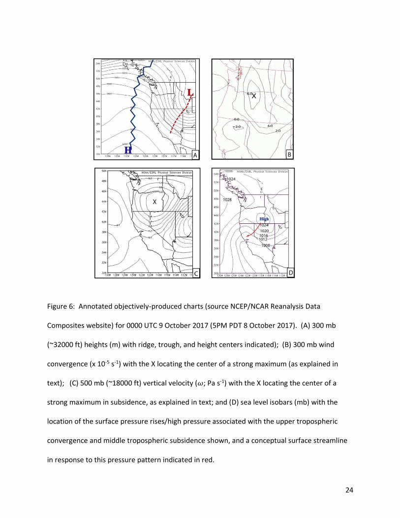
States. By the late afternoon of October 8, 2017 (0000 UTC 9 October 2017), the upstream

ridge in the upper troposphere (300 mb level; ~32000 ft) was located over the Pacific

Northwest and the trough over Nevada (Fig. 6a). Upper tropospheric convergence was

occurring in between the ridge and the trough (Fig. 6b). As expected from mass conservation,

compensating mid tropospheric (500 mb level; ~18000 ft) subsidence was strong (Fig. 6c). The

associated lower troposphere pressure rises produced a high-pressure area over the Pacific

Northwest associated with surface pressure gradients directed offshore over north-central

California (objectively drawn analysis from the NCEP/NCAR Reanalysis Data in Fig. 6d and

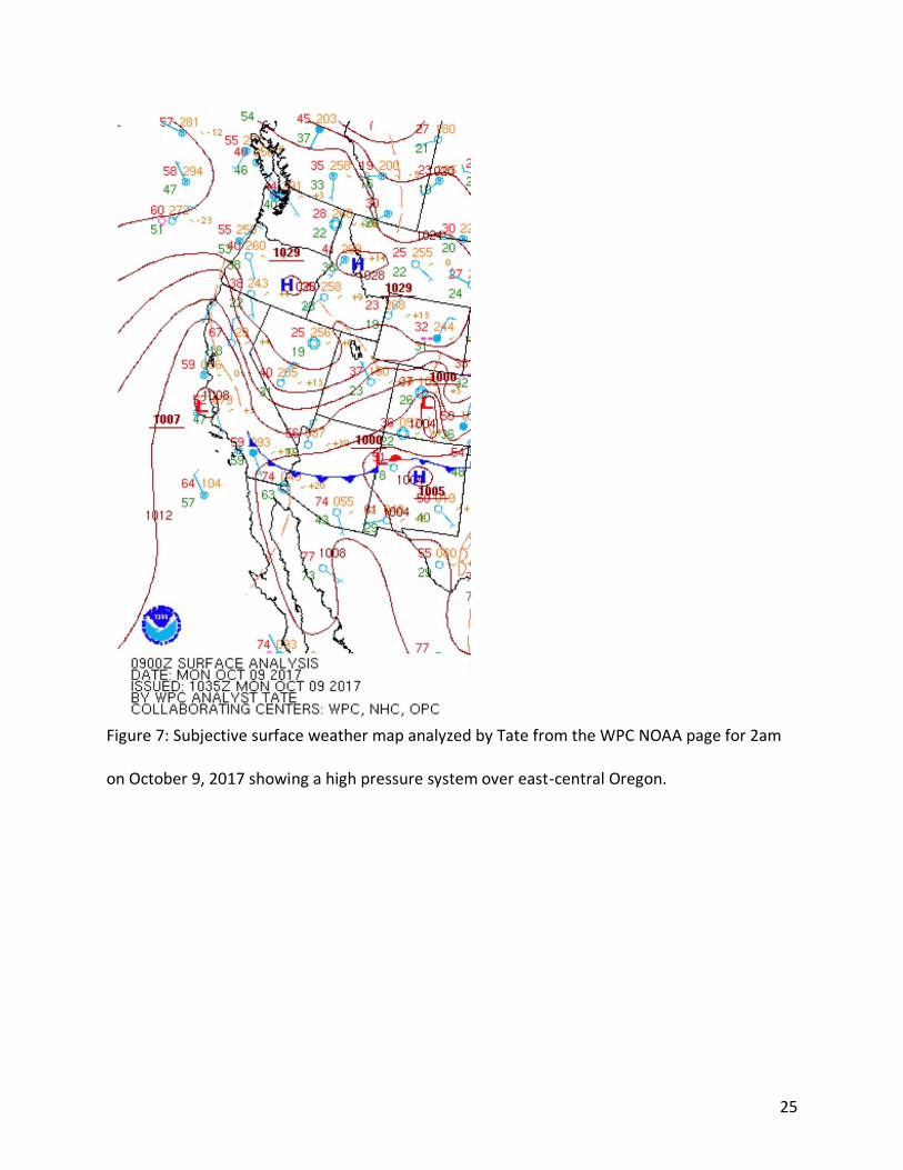
subjective analysis in Fig. 7).

The surface pressure pattern was associated with strong northeasterly flow at nearly

right angles to the ridge lines of the Mayacamas Mountains (see Figs. 2 and 8). This brought

warm dry air into the area with relative humidity’s as low as 10% (NWS,2017).

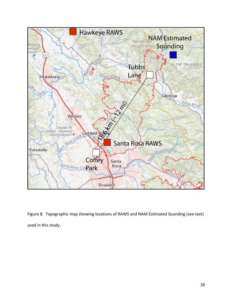
Actual weather observations were collected near the fire areas from the Hawkeye and Santa

Rosa Remote Automated Weather Stations (RAWS) (see Fig. 8 for locations). Flow was strong at

Hawkeye (Table 1), which recorded a wind gust of 35 m s-1 (78mph) at 11pm on October 8 and

Santa Rosa (Table 2), which recorded a peak gust of 30 m s-1 (68 mph). The Santa Rosa RAWS

also recorded a sharp temperature rise to 33°C (91°F) at around 3am, probably related to the

fire, since temperatures in other areas in the region were in the 16-20°C (60-70°F) range.

11

3.2 Mesoscale Thermodynamic Controls

The Diablo Wind pattern discussed in Section 2.2 is associated with strong subsidence in

the lower mid-troposphere. Such subsidence is typically associated with the development of a

thermal stratification called a “subsidence inversion” (Barry and Chorley, 2010, p. 172). The

northeasterly flow in the lowest portion of the troposphere that occurs in this pattern

encounters the mountain ranges in north-central California with a thermal stratification that

features an inversion or stable layer at elevations somewhat above the tops of the coastal

mountains.

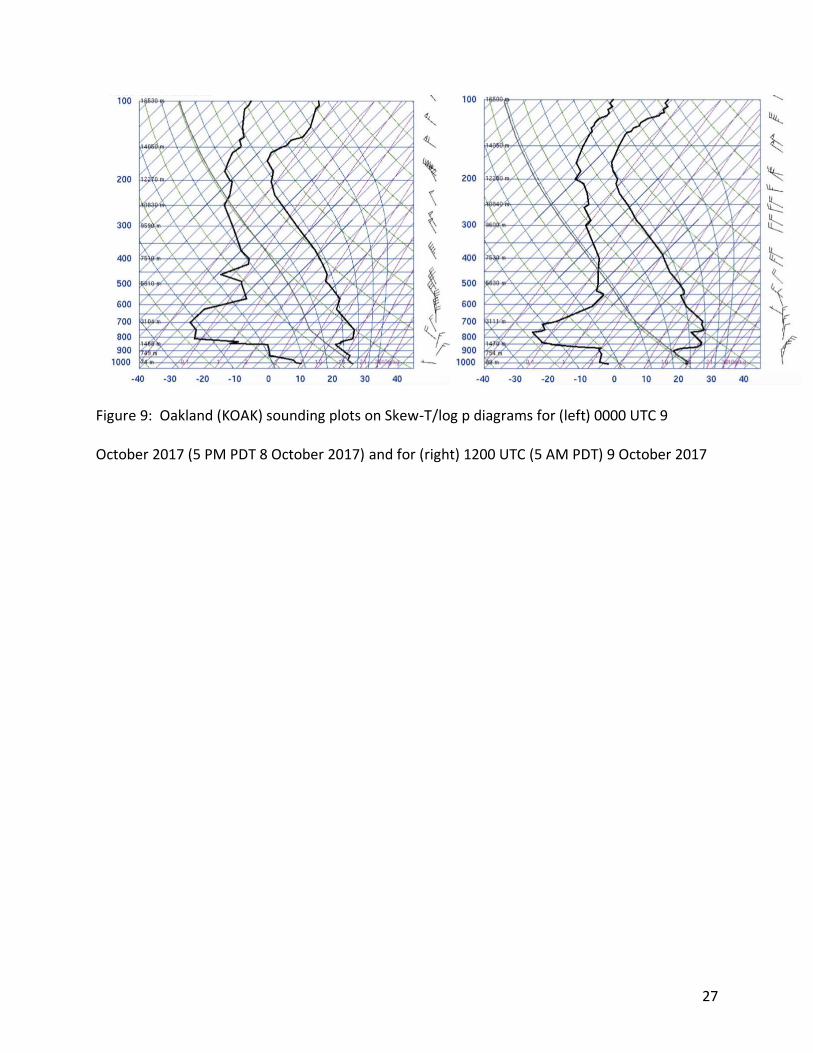
The subsidence inversion can be visualized by examination of atmospheric soundings

that show the vertical lapse of temperature, dew point, and wind. The 0000 UTC and 1200 UTC

9 October Oakland soundings (Fig. 9) show a strong inversion in the lower mid-troposphere.

This lowered from around an elevation of 1500 m (5,000 ft) to an elevation of around 1300 m

(4,300 ft) in that 12 h period. This is significant because the elevation of the ridges of the

western range of the Mayacamas Mountains is between 1200 and 1600 m (4,000 and 5,300 ft).

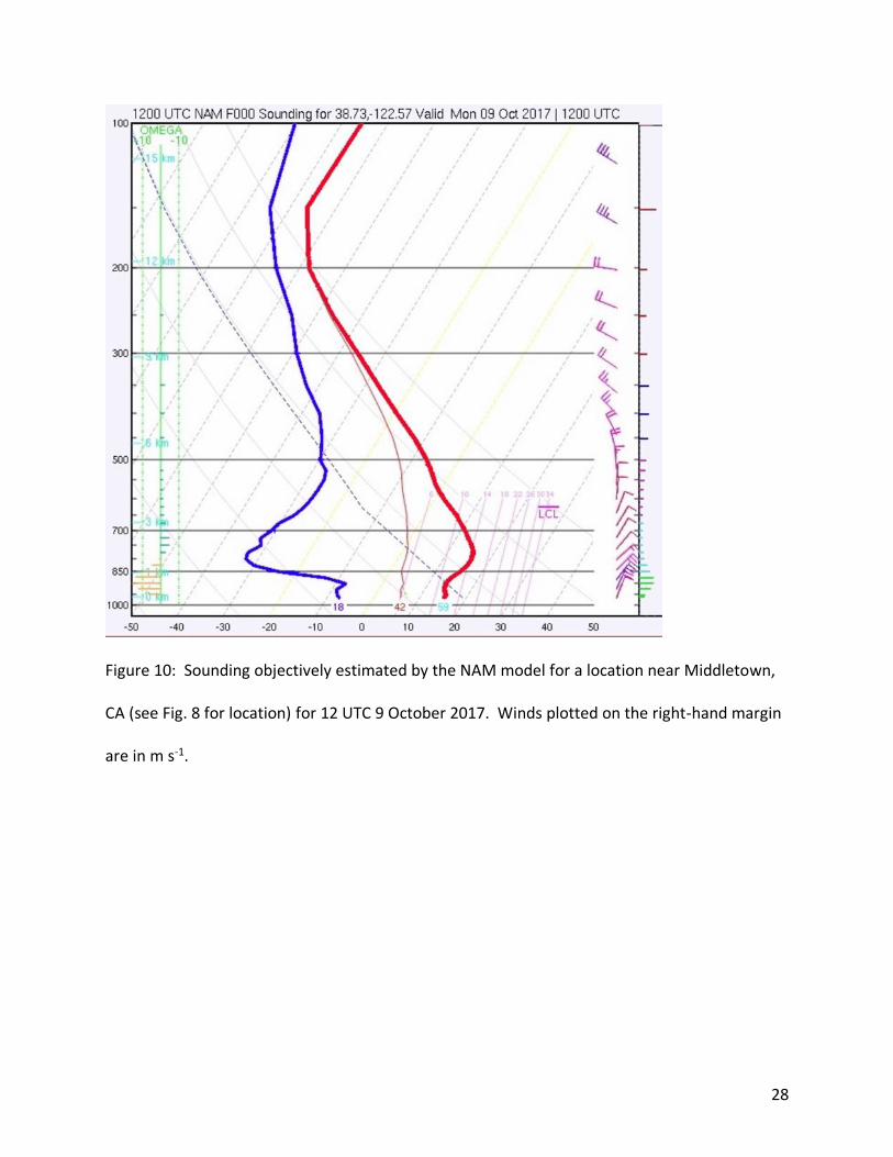
It is also noteworthy that a sounding objectively obtained from the NAM estimated for a

location upwind of the Mayacamas Mountains near Middletown (see Fig. 8 for location) for

1200 UTC 9 October (Fig. 10) reveals that a temperature inversion around 900mb, near the

crest of the Mayacamas Mountains, was present the morning of the rapid spread of the Tubbs

Fire into the Coffey Park neighborhood of Santa Rosa. The location of the NAM estimated

sounding is important since it was in the inflow region of the fire area, as depicted in Figs. 1 and

2.

12

The calculation of the Froude Number in Section 2.3 was made on the basis of the stable

layer’s location at 12 UTC as shown in Figs. 9 and 10. The estimate of wind speed of the flow

orthogonal to the Mayacamas Mountains by averaging the wind speeds shown in the inversion

layer shown in Fig. 10. The magnitude of the stability was determined by calculation of the

Brunt-Vaisala Frequency, N:

𝑁 = (𝑔

𝜃

𝜕𝜃

𝜕𝑧)1/2

(Equation 2)

where is the potential temperature obtained from the soundings. These values were

substituted into the National Center for Atmospheric Research’s (NCAR) online Froude Number

calculator at http://www.meted.ucar.edu/mesoprim/lff/froude_calc.htm

Given the difference in elevation of the northern Napa Valley and the Mayacamas

Range, the Brunt-Vaisala Frequency was 0.018, mountain deflection depth of ~1100 m, and

isothermal stable layer at top of mountain, and the Froude Number was near 1 (0.99). Thus, the

wind pattern and thermodynamic structure as estimated by the Froude Number that occurred

with the Diablo Wind pattern that took place on October 8-9 in the Tubbs Fire area favored the

development of strong ridge-top and lee-side downslope winds associated with the "hydraulic

jump" phenomenon.

While hydraulic jumps can occur with Santa Ana winds, the same thermodynamic

structure that occurs with them typically favors "gap" flow more frequently (Gabersek and

Durran, 2006). Thus, Santa Ana Winds are strongest in canyons, whereas a Diablo Wind event is

first noted and blows strongest atop ridges and on the western slopes of the various mountain

peaks and ridges around the Bay Area. It should be pointed out that channeling by canyons can

13

also be significant and cannot be completely discounted as an additional contributing factor in

the Tubbs Fire case.

3.3 Aspects of Mesoscale Controls Leading to Ducting

Local observations combined with synoptic and thermodynamic controls on 8-9 October

2017 support that the Diablo Wind pattern was present. Both the 0000 UTC and 1200 UTC 9

October Oakland soundings (Fig. 7) and a sounding objectively obtained from the North

American Model (NAM) estimated for a location upwind of the Mayacamas Mountains near

Middletown at 1200 UTC 9 October (Fig. 8) reveal that a temperature inversion around 900mb,

near the crest of the Mayacamas Mountains, was present the night and morning of the Tubbs

Fire. This inversion stabilizes the atmosphere and acts like a lid above which surface air parcels

will resist rising.

As discussed above, actual weather observations were collected near the fire areas from

the Hawkeye and Santa Rosa Remote Automated Weather Stations (RAWS) (see Fig. 6 for

locations). The range of the peak wind speeds at these stations seem consistent with the

hypothesized accelerated, constrained flow over the top and down the lee slopes of the

Mayacamas Mountains as well.

4. WRF Simulation

4.1 General Background on WRF Model The WRF-ARW Model, developed and supported by National Center for Atmospheric

Research, can make forecasts of weather variables on user-specified bounded regions in space

(domains) with high spatial and temporal resolution (Skamarock and et al., 2008). The WRF-

ARW is a high-resolution Numerical Weather Prediction (NWP) model that can be configured to

14

run in different geographic domains and with different resolutions. The model solves a set of

equations that describe how the state of the atmosphere, represented on a three-dimensional

grid of points, changes over time at a series of discrete times over a domain the consists of a

number of grid points.

To calculate a forecast, the model requires two kinds of information: (1) the state of the

atmosphere at the grid of points at the starting time (i.e., initial conditions); and (2) the state of

the atmosphere at grid points on the boundary of the forecast domain at all subsequent

forecast times (i.e., boundary conditions). For this study, this initialization information was

obtained from the NAM model initialization data obtained online from

https://catalog.data.gov/dataset/north-american-mesoscale-forecast-system-nam-12-km

4.2 Procedure to Simulate Horizontal and Vertical Motions During the Event using WRF Model

To depict whether a hydraulic jump was present, I used the analysis grids we named

NorCal, North Bay, and Mayacamas Mountains domains nested within each other with 10, 3.3,

and 1.1 km resolutions, respectively. The dates and times of the simulation are dynamic

initialization (00Z Oct 8, 2017), effective simulation start (06Z Oct 8, 2017), and simulation end

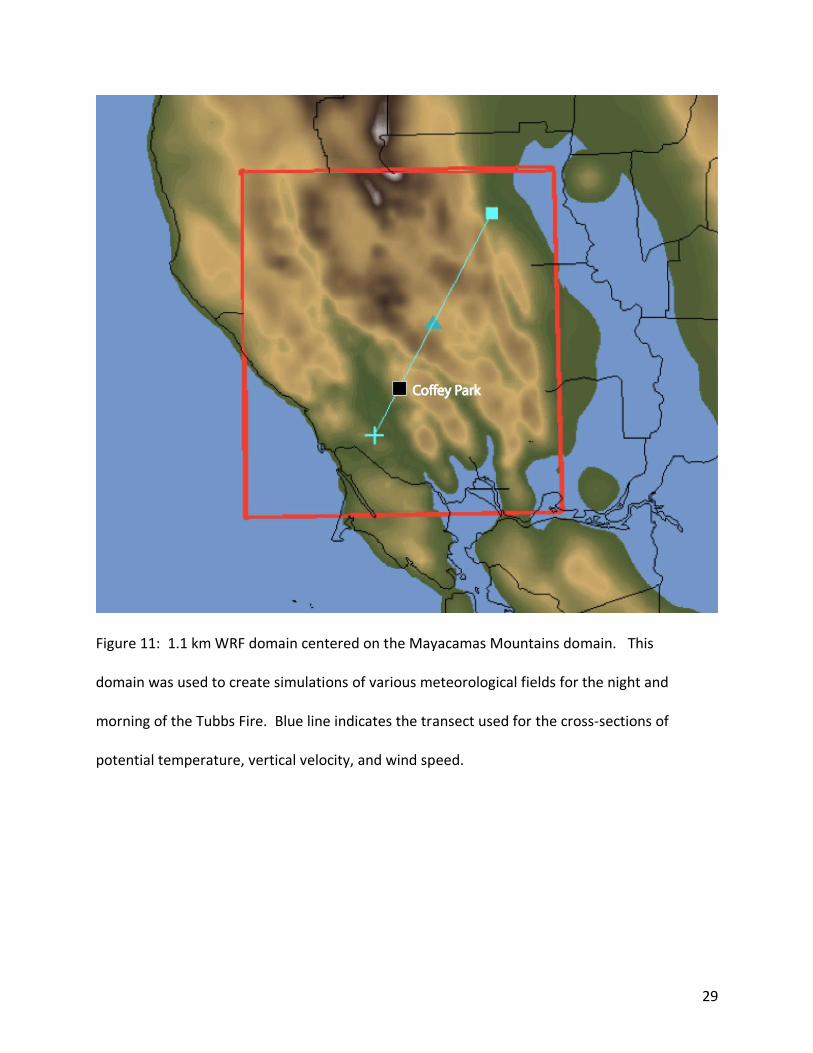
(18Z Oct 9, 2017). A transect in the Mayacamas Mountains domain was used to create a cross-

section of the atmosphere that has a vertical resolution to 3,000m above the surface (Fig. 11).

This transect was designed to be tangent to the fire path from Tubbs Lane to the Coffey Park

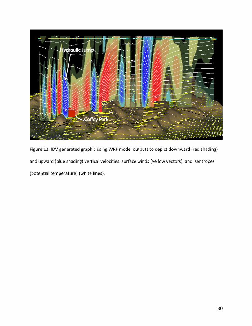
neighborhood, as shown in Fig. 2. Using the Integrated Data Viewer (IDV) I constructed a vertical

cross-section with ‘isosurfaces’ of vertical velocities (+-0,.25 m/s), of potential temperature

(isentropes), and wind vectors 10 meters above the earth’s surface, at 3am October 9, the night

15

of the Tubbs Fire (Fig. 12). This is the time nominally attributed to that the fire entered the Coffee

Park neighborhood, as discussed in section 2.1 above,

4.3 Results of Simulation

Durran (1990) and many others have described the pattern of isentropes and vertical

velocities associated with hydraulic jumps. Key features include a packing of the isentropes

beneath the inversion, ducting of the wind and isentropes from the ridge top downwind along

the lee slopes, and a lofting of the packed isentropes downwind of the lee slope. Terrain-parallel

winds should be strong from ridge top down the lee slopes, with a virtual calm or horizontal wind

minimum under the hydraulic jump itself. All of these features are consistent with the pattern

schematically shown in Fig. 5.

The results of the simulation, shown in Fig. 12, reveal that isentropes over of the Western

Mayacamas Mountain range were tightly packed together over the range and ducted on the

leeward side of the range, followed by a jump, just after Coffey Park. Surface winds were strong

just leeward of the mountain followed by calm winds west of Coffey Park. The overlain vertical

velocities show strong subsidence leeward of the range followed by rebound just after Coffey

Park. These aspects of the simulation output are consistent with the surface wind observations

at the RAWS and also corroborate that a hydraulic jump was present the night of the Tubbs Fire.

It should be pointed out that there were no actual observations along the transect except the

Santa Rosa RAWS (Fig. 8). So caution should be exhibited in making assumptions about the real

wind flow along the transect. Nevertheless, the simulation is powerful evidence that the

hydraulic jump phenomenon was a player in the Tubbs Fire weather pattern.

16

It should also be pointed out that the simulation suggests an even stronger hydraulic jump

over the northern Napa Valley in the vicinity of Tubbs Lane. The downslope ducting in the lee of

Mt. Saint Helena was even more pronounced there than that in the Coffey Park neighborhood,

suggesting that this might have played a role in the initial fast fire spread from the Tubbs Lane

ignition point, but that hypothesis is beyond the scope of this study.

5. Conclusions and Discussion

On the evening of October 8, 2017, a series of wildfires developed and spread over

nearly 250,000 acres in Napa and Sonoma Counties of Northern California (Fig. 1). Analyses of

synoptic, mesoscale, and thermodynamic conditions during the first 24 hours of the largest of

these, the Tubbs Fire, indicate that the weather pattern corresponded to the “Diablo Wind

Pattern”, characterized by strong offshore flow over the northern San Francisco Bay Region.

The observed flow in the boundary layer was at right angles to terrain features in the

Mayacamas Mountains at the same time that actual and objectively-produced model soundings

showed a strong stable layer/temperature inversion near the top of the range. These

conditions met the criteria described in the literature for an enhanced downslope

windstorm/hydraulic jump.

WRF-ARW simulations summarized above support the hypothesis presented here,

namely, that ducted, augmented flow occurred over the ridge tops and down the southwestern

slopes of the mountains into the Coffey Park neighborhood of Santa Rosa. The model produced

realistic values of wind speeds (when compared to actual observations) over the Mayacamas

Mountains domain. Strong downward and upward vertical velocities of the simulation

17

confirmed the hypothesis that the hydraulic jump phenomenon did occur for the conditions

that existed in the area on 8-9 October 2017.

6. References

Barry, R. G. and Chorley, R.J., 2010: Atmosphere, Weather, and Climate. Taylor & Francis, 516 pp. CAL Fire, 2018a: Top 20 Most Destructive Wildfires. State of California Online Access to Fact Sheets, http://www.fire.ca.gov/communications/downloads/fact_sheets/Top20_Destruction.pdf CAL Fire, 2018b: Incident Report of Camp Fire. State of California Online Access to Incident Information, http://www.fire.ca.gov/current_incidents/incidentdetails/Index/2277 CAL Fire, 2017: Incident Report of LNU Complex. State of California Online Access to Perimeter Maps,http://calfireforestry.maps.arcgis.com/apps/webappviewer/index.html?id=58dc77306bf448c6ac5f756af51f3ae5 Durran, D., 1990: Mountain Waves and Downslope Winds. Meteor. Mon., Vol. 23, 59-83. (https://atmos.washington.edu/~durrand/pdfs/AMS/Durran_MountainWavesandDownslopeWinds.pdf) Gabersek, S. and Durran, D., 2006: "The dynamics of gap flow over idealized topography. Part II: Effects of rotation and surface friction". Journal of the Atmospheric Sciences. 26: 2720–2739. Jones, C., Fujoka, F, and L. Carvaiho, 2010: Forecast Skill of Synoptic Conditions Associated with Santa Ana Winds in Southern California. Mon. Wea. Rev., 138, 4528-4541. Lied, N. T., 1964: Stationary hydraulic jumps in a katabatic flow near Davis, Antarctica, 1961. Aust. Meteor. Mag., 47, 40–51 Markowski, P. and Y. Richardson, 2010: Mesoscale Meteorology in Midlatitudes. Wiley-Blackwell, 407 pp. McCutchan, M. H., and M. J. Schroeder, 1973: Classification of meteorological patterns in Southern California by discriminant analysis. J. Appl. Meteor., 12, 571–577. Monteverdi, J.P., 1973: The Santa Ana weather type and extreme fire hazard in the Oakland-Berkeley Hills. WEATHERWISE. 26, 118-121.

18

National Weather Service, 2017: Sonoma County Wildfires. Internal Incident Report by Matt Mehle, National Weather Service Forecast Office, Monterey, 39 pp. Rosenthal, J., 1972: Point Mugu Forecasters Handbook. Chapter 5. Santa Ana Winds. PMRTP721. Pacific Missile Range, Point Mugu, California, 278 pp. Skamarock et al. 2008 "A Description of the Advanced Research WRF Version 3." Chapters 5 & 6. University Corporation for Atmospheric Research. June 2008. http://www2.mmm.ucar.edu/wrf/users/docs/arw_v3.pdf. WERT, 2017: Tubbs Fire Assessment Report. Report #CA-LNU-010104. (Available Online at http://www.fire.ca.gov/communications/downloads/Watershed_reports/20171115_TubbsWERT.pdf)

7. Tables

Table 1: Hawkeye RAWS daily summary data for October 8-9, 2017.

Table 2: Santa Rosa RAWS daily summary data for October 9th, 2017.

19

8. Figures

Figure 1: Tubbs Fire burn map (from Watershed Emergency Response Team [WERT], 2017)

20

Figure 2: General location map showing location of Coffey Park neighborhood, the Tubbs Lane

fire start location, and the Mayacamas Mountains. Red outlined areas represent the final

locations of the fire affected areas from the 2017 fires (Cal Fire, 2017)

21

Figure 3: Comparison of Perimeters of Tubbs Fire and C. Hanly Fire (extracted from National

Weather Service, 2017)

22

Figure 4: Charts for the 1200 UTC 27 October 1970 Diablo Wind Pattern (a) 500mb height map

(dm); and (b) Surface isobars (mb) and fronts from Monteverdi (1973), his Figs. 2a and 2b.

23

Figure 5: Schematic chart (adapted from EuMeTrain, 2018) showing a well-developed hydraulic

jump. Wind streamlines (closeness is related to speed) are given for an easterly wind at right

angles to prevailing topography when an inversion layer just tops the mountains. Isentropes

(contours of potential temperature) (not shown) would be parallel to streamlines with similar

spacing

24

Figure 6: Annotated objectively-produced charts (source NCEP/NCAR Reanalysis Data

Composites website) for 0000 UTC 9 October 2017 (5PM PDT 8 October 2017). (A) 300 mb

(~32000 ft) heights (m) with ridge, trough, and height centers indicated); (B) 300 mb wind

convergence (x 10-5 s-1) with the X locating the center of a strong maximum (as explained in

text); (C) 500 mb (~18000 ft) vertical velocity (𝜔; Pa s-1) with the X locating the center of a

strong maximum in subsidence, as explained in text; and (D) sea level isobars (mb) with the

location of the surface pressure rises/high pressure associated with the upper tropospheric

convergence and middle tropospheric subsidence shown, and a conceptual surface streamline

in response to this pressure pattern indicated in red.

25

Figure 7: Subjective surface weather map analyzed by Tate from the WPC NOAA page for 2am

on October 9, 2017 showing a high pressure system over east-central Oregon.

26

Figure 8: Topographic map showing locations of RAWS and NAM Estimated Sounding (see text)

used in this study.

27

Figure 9: Oakland (KOAK) sounding plots on Skew-T/log p diagrams for (left) 0000 UTC 9

October 2017 (5 PM PDT 8 October 2017) and for (right) 1200 UTC (5 AM PDT) 9 October 2017

28

Figure 10: Sounding objectively estimated by the NAM model for a location near Middletown,

CA (see Fig. 8 for location) for 12 UTC 9 October 2017. Winds plotted on the right-hand margin

are in m s-1.

29

Figure 11: 1.1 km WRF domain centered on the Mayacamas Mountains domain. This

domain was used to create simulations of various meteorological fields for the night and

morning of the Tubbs Fire. Blue line indicates the transect used for the cross-sections of

potential temperature, vertical velocity, and wind speed.

30

Figure 12: IDV generated graphic using WRF model outputs to depict downward (red shading)

and upward (blue shading) vertical velocities, surface winds (yellow vectors), and isentropes

(potential temperature) (white lines).