The Schrodinger Equation and Postulates

Common operators in QM:

Potential Energy Often depends on position operator:

Kinetic Energy 1-D case:

3-D case

Time

Total energy = Hamiltonian

To find out about the particle one solves the Schrödinger Equation:

Suppose the potential does not depend on t. Thus H and E do not change with time.

Whenever we have a function of multi variables we will attempt to separate them. In the wavefunction this works into a product:

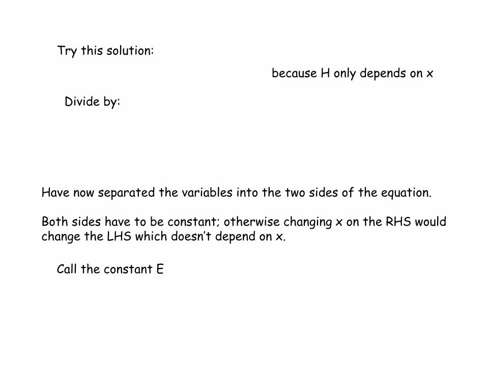
Try this solution:

because H only depends on x

Divide by:

Have now separated the variables into the two sides of the equation. Both sides have to be constant; otherwise changing x on the RHS would change the LHS which doesn’t depend on x.

Call the constant E

LHS:

This leads to solutions of the form:

RHS:

This is the time-independent Schrodinger wave equation and it is an eigenvalue equation

is a stationary state; i.e., solution of the time-independent equation times f(t) because the energy does not change in time.

The magnitude of Ψ(x,t) does not change in time:

The phase changes in time, not the magnitude

The general solution of the Schrodinger wave equation is a linear combination of the separable solutions. The Schrodinger equation yields an infinite collection of solutions: Ψ1(x), Ψ2(x), …, each with its own separation constant En.

For each E, there is an eigenfunction

The general solution of the Schrodinger equation is a linear combination of these. We will do applications of these later on.

The postulates of Quantum Mechanics

Postulate 1: The state of a QM system is completely specified by a wavefunction

Ψ(x1,t1) is assumed to be normalized. Why?

This assumes:

Ψ(x,t) and its first derivative must be single-valued, otherwise there would 2 or more values for the probability of the particle being at the same location.

Ψ(x,t) must be continuous. The exception is that the first derivative can be discontinuous if the potential is infinite; otherwise the derivative in the Schrodinger equation would be infinite.

The probability that the particle will be found at time t1 in a spatial interval of width dx centered at x1 is given by

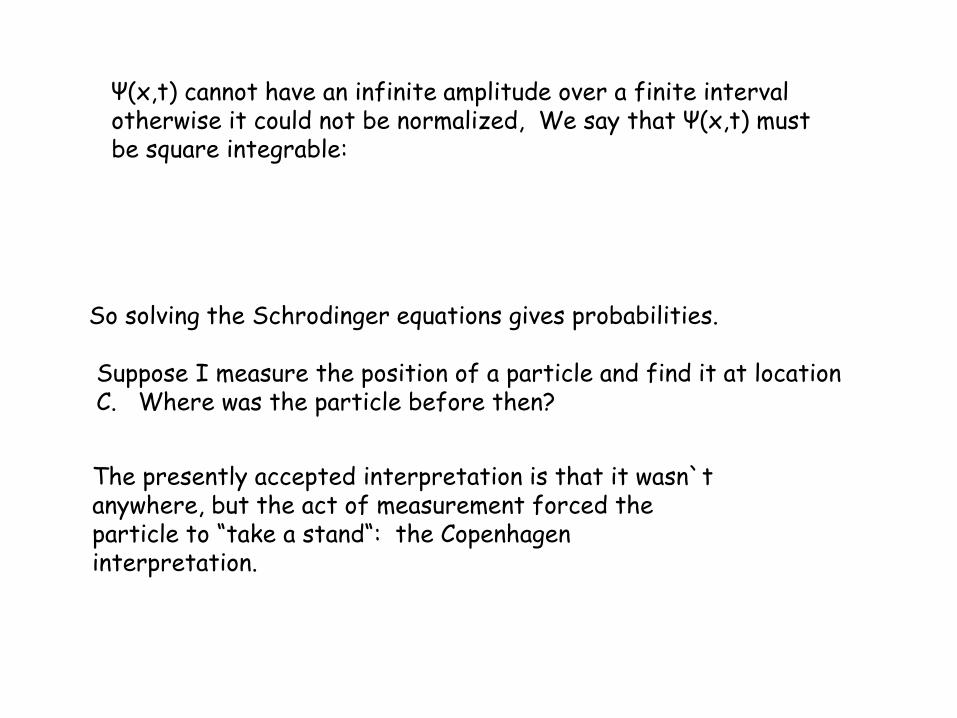
Ψ(x,t) cannot have an infinite amplitude over a finite interval otherwise it could not be normalized, We say that Ψ(x,t) must be square integrable:

So solving the Schrodinger equations gives probabilities.

Suppose I measure the position of a particle and find it at location C. Where was the particle before then?

The presently accepted interpretation is that it wasn`t anywhere, but the act of measurement forced the particle to “take a stand“: the Copenhagen interpretation.

Postulate 2: For every measurable property of the system there exists a corresponding Hermitian operator:

Postulate 3: In any single measurement of an observable that corresponds to an operator the only values that will measured are the eigenvalues of that operator.

A

Postulate 4: If the system is in a state described by the wavefunction ø(x,t) and the value of the observable a is measured ounce, each time on many identically prepared systems the average (expectation) value of all these measurements is:

The denominator = 1 if ø is normalized

Postulate 5: The evolution in time of a QM system in governed by the time-dependent Schrodinger equation:

There are 2 cases here:

(i) If Ψj is an eigenfunction of A then only aj will be measured.

(ii) If Ψ is not an eigenfunction we can expand it in terms of functions {øn} which eigenfunctions of the operator

Recall:

The eigenfunctions of a Hermitian operator are orthogonal

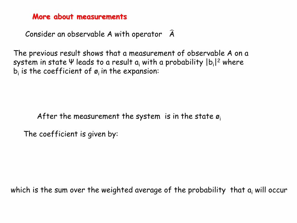
More about measurements

Consider an observable A with operator A

The previous result shows that a measurement of observable A on a system in state Ψ leads to a result ai with a probability |bi|

2 where bi is the coefficient of øi in the expansion:

After the measurement the system is in the state øi

The coefficient is given by:

which is the sum over the weighted average of the probability that ai will occur

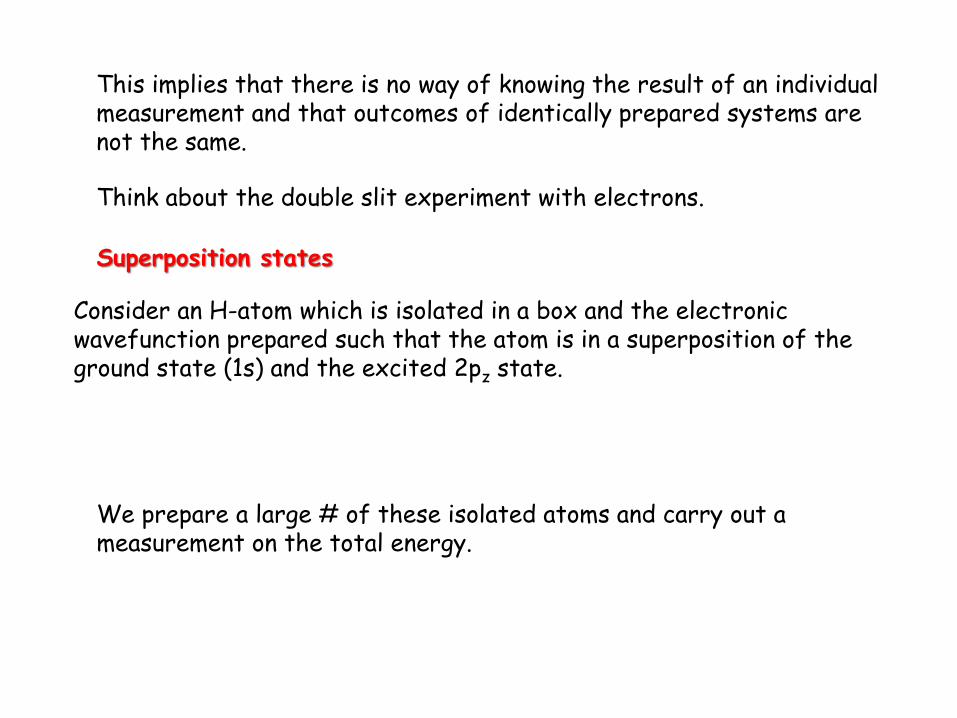
This implies that there is no way of knowing the result of an individual measurement and that outcomes of identically prepared systems are not the same.

Think about the double slit experiment with electrons.

Superposition states

Consider an H-atom which is isolated in a box and the electronic wavefunction prepared such that the atom is in a superposition of the ground state (1s) and the excited 2pz state.

We prepare a large # of these isolated atoms and carry out a measurement on the total energy.

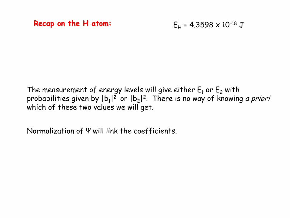
Recap on the H atom: EH = 4.3598 x 10-18 J

The measurement of energy levels will give either E1 or E2 with probabilities given by |b1|

2 or |b2|2. There is no way of knowing a priori

which of these two values we will get.

Normalization of Ψ will link the coefficients.

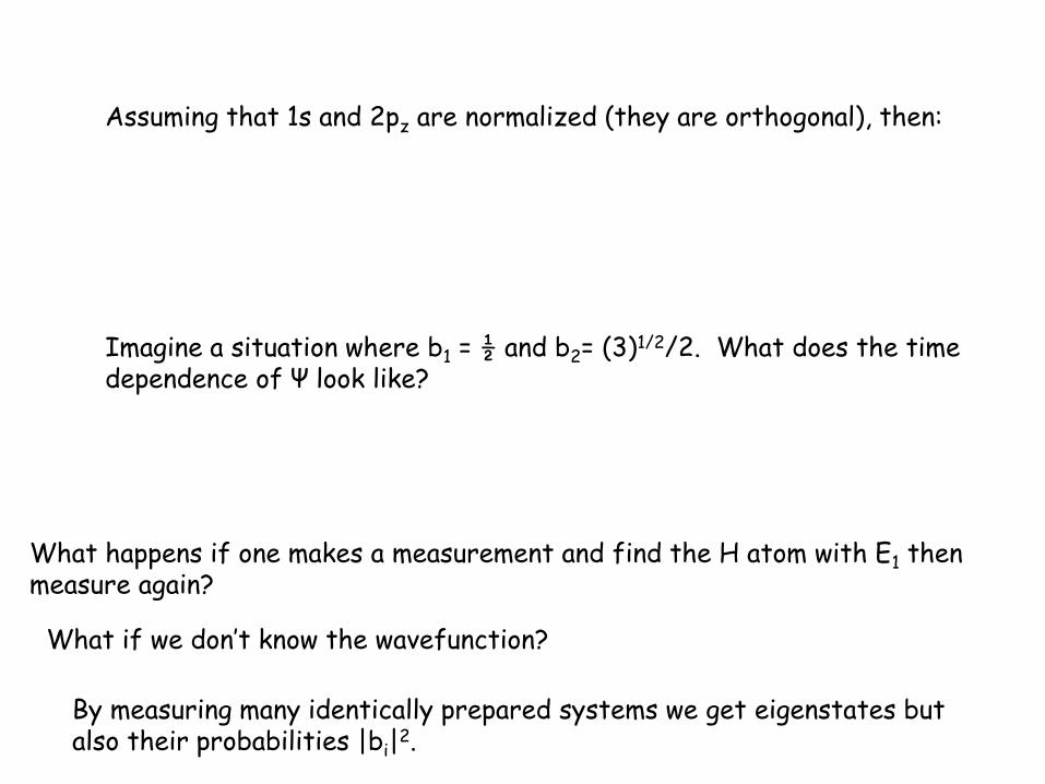
Assuming that 1s and 2pz are normalized (they are orthogonal), then:

Imagine a situation where b1 = ½ and b2= (3)1/2/2. What does the time dependence of Ψ look like?

What happens if one makes a measurement and find the H atom with E1 then measure again?

What if we don’t know the wavefunction?

By measuring many identically prepared systems we get eigenstates but also their probabilities |bi|

2.

Unfortunately this is done within a multiplication factor eiθ 0 ≤ θ ≤ 2π. We cannot construct the exact superposition state from experimental results.

Complete sets

The eigenfunctions of a Hermitian operator form a complete set (no proof will be given).

If fj is an eigenfunction of an operator A with eigenvalue aj.

Any function g can therefore be written as:

The advantage is this allows us to determine the effects of A on g more easily.

Thus any other function can be expanded in terms of a complete set.

For vectors an example of such a complete set is the set of Cartesian unit vectors: i, j, k. Any other vector can be written as a linear combination if i, j, and k.

A special case: When all eigenfunctions are degenerate, and linear combination is also an eigenfunction.

Another example of the complete set is a Fourier series where the functions sin(mu) and cos(nu), m, n = 0.1, …, ∞ form a complete orthogonal set over [0,2π]. Any periodic function with a period of 2π can be expanded in a Fourier series.

To find the coefficients multiply both sides by the appropriate basis function and integrate.

For example to find d2 multiply by cos(2x)

All integrals are 0 (orthogonality) and only 1 term survives on the RHS.

Example: Try expanding the function x2 + 2 over the interval [0, 2π] and calculate d0 and d1.

Integration by parts (a little work) yields d1π = 8π; that is d1 = 8.

By extension to complete sets in general:

If