The Schwarzschild Metric and Applications 1

Analytic solutions of Einstein's equations are hard to come by.  It's easier in situations that exhibit symmetries.

1916:  Karl Schwarzschild sought the metric describing the static, spherically symmetric spacetime surrounding a spherically symmetric mass distribution.

A static spacetime is one for which there exists a time coordinate t such that

i)   all the components of g

 are independent of t

ii)  the line element ds2 is invariant under the transformation  t  ­t

A spacetime that satisfies (i) but not (ii) is called stationary.  An example is a rotating azimuthally symmetric mass distribution.

The metric for a static spacetime has the form

where xi are the spatial coordinates and dl2 is a time­independent spatial metric.  Cross­terms dt dxi are missing because their presence would violate condition (ii).

The Ricci tensor for this metric is diagonal, with components

Primes denote differentiation with respect to r.SP 10.1

[Note:  The Kerr metric, which describes the spacetime outside a rotating axisymmetric mass distribution, contains a term ∝ dt d.]

To preserve spherical symmetry, dl2 can be distorted from the flat­space metric only in the radial direction.  In flat space,  (1)  r is the distance from the origin and  (2)  4r2 is the area of a sphere.  Let's define r such that (2) remains true but (1) can be violated.  Then,

A(xi)  A(r) in cases of spherical symmetry.

2

The region outside the spherically symmetric mass distribution is empty.The vacuum Einstein equations are R

 = 0.  To find A(r) and B(r):

3

2.  Substitute this result for B in the expression for R

, set it equal to zero,     

     and solve for A:

(k is another constant of integration)

Thus,

Note:  We only used the sum of Rtt and R

rr to solve for A and B.  We must

also verify that Rtt and R

rr vanish individually  (exercise for home).

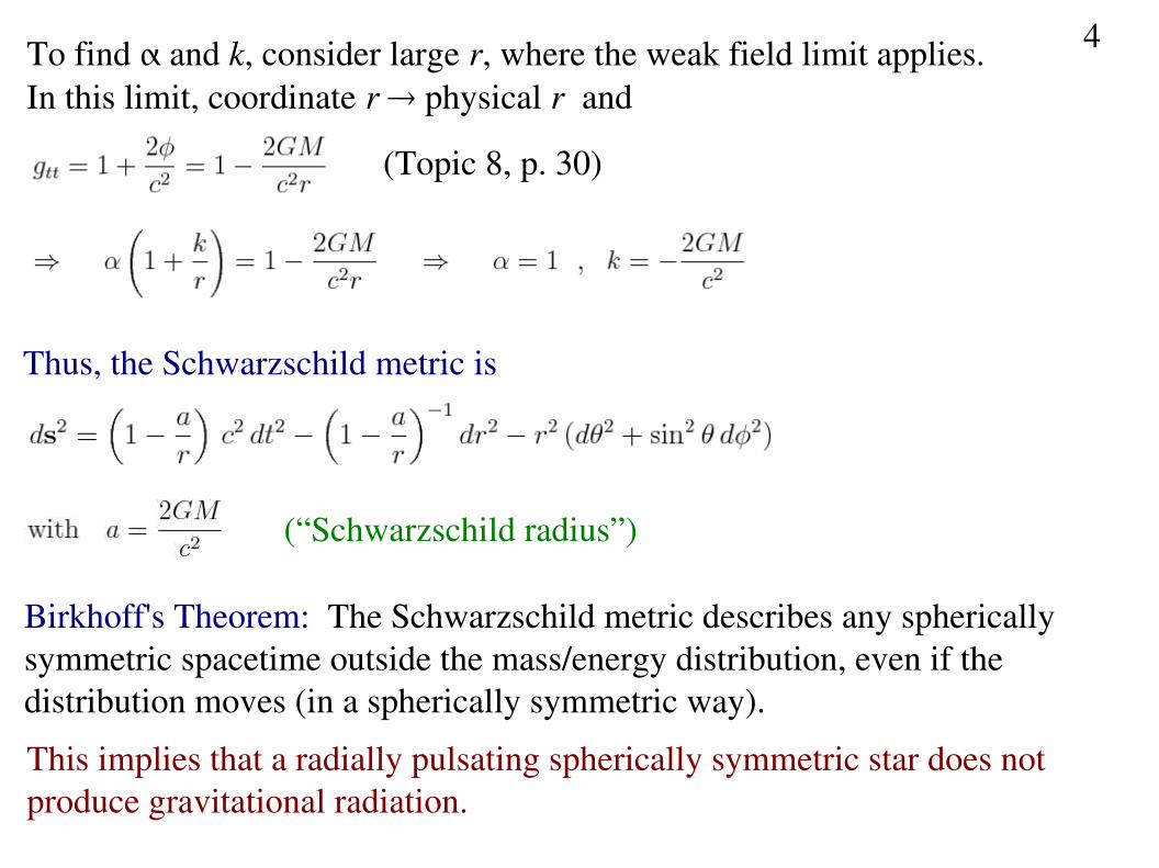
To find  and k, consider large r, where the weak field limit applies.In this limit, coordinate r  physical r  and 

(Topic 8, p. 30)

4

Thus, the Schwarzschild metric is

(“Schwarzschild radius”)

Birkhoff's Theorem:  The Schwarzschild metric describes any spherically symmetric spacetime outside the mass/energy distribution, even if the distribution moves (in a spherically symmetric way).  

This implies that a radially pulsating spherically symmetric star does notproduce gravitational radiation.

Measuring distances and times:

1.  The metric blows up at r = a    =>   we need different coords to      describe the region r ≤ a, if this region is empty.

2.  The spatial and temporal parts of the metric are separate.  For static     spacetimes, such coords can always be chosen.

a = 2.9 km  for the Sun's mass  and  a = 0.88 cm  for the Earth's mass.

5As noted on p. 2, if t and r are constant, then the metric describes thesurface of a sphere, with polar angle   and azimuthal angle  , and  surface area 4r2.

Thus, r is known as the “area distance”.

As r   ∞ ,  the metric becomes Minkowskian   (“asymptotic flatness”)

3.  When a = 0, the metric is flat.  When a > 0, both the spatial and       temporal parts are curved.

4.  When a > 0, the coord distance (i.e., area dist), r, does not measure      the radial distance R btwn 2 points with the same , :

Lampshadeanalogy:

dR

dr

Distance from one circleto the next is dR, but increase in circumferenceradius is dr.

The center of the circle(or sphere) doesn't even have to be in the space!

6

5.  The proper time elapsed on a clock at a fixed position in space is:

Stationary clocks do not tick coordinate time!  (as we saw in our earlier thought experiment)

Gravitational frequency shift:

Suppose a light signal is sent from 

Coordinate time of emission = tE

,  reception = tR

ds2 = 0   =>

With u an affine parameter for the null geodesic of the signal:  

7

SP 10.2

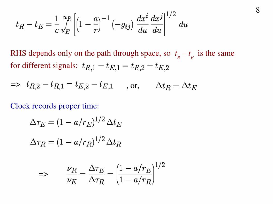
RHS depends only on the path through space, so  tR – t

E  is the same

for different signals:   

=> , or, 

Clock records proper time:

=>

8

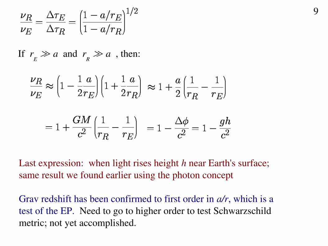
If  rE ≫ a  and  r

R ≫ a  , then:

Last expression:  when light rises height h near Earth's surface; same result we found earlier using the photon concept

Grav redshift has been confirmed to first order in a/r, which is a test of the EP.  Need to go to higher order to test Schwarzschild metric; not yet accomplished.

9

Solar System Tests of GR

1.  Precession of Mercury's perihelion

Start with the Newtonian theory of orbits:

Specific angular momentum,  h = r × v

r × v = const  =>  particle moves in a single plane (⊥ h); we'll                              assume  = /2

Total specific energy (kinetic plus potential) is 

With ,

10

;

Define u = 1/r :

Energy equation becomes:

Substituting from the angular momentum  equation:

Differentiate:

11

=>

Solution:

=>

Circle if  e = 0,  ellipse if  0 ≤ e < 1  (as for planets orbiting the Sun)

Perihelion (closest approach to Sun) occurs when   = 0  (maximizes

denominator in expression for r)

12

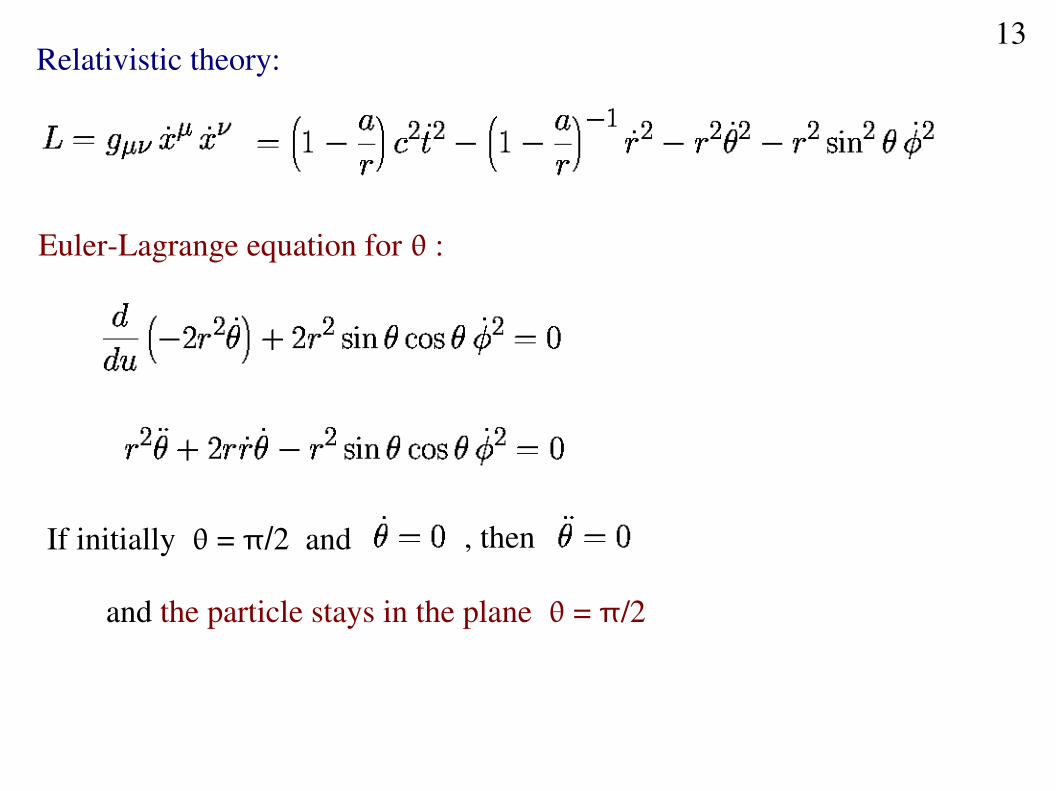
Relativistic theory:

Euler­Lagrange equation for  :

If initially   = /2  and , then 

and the particle stays in the plane   = /2

13

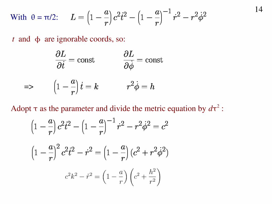
With   = /2:

t  and    are ignorable coords, so:

=>

Adopt  as the parameter and divide the metric equation by d2 :

14

Again, define  u = 1/r :

Differentiate:   

15

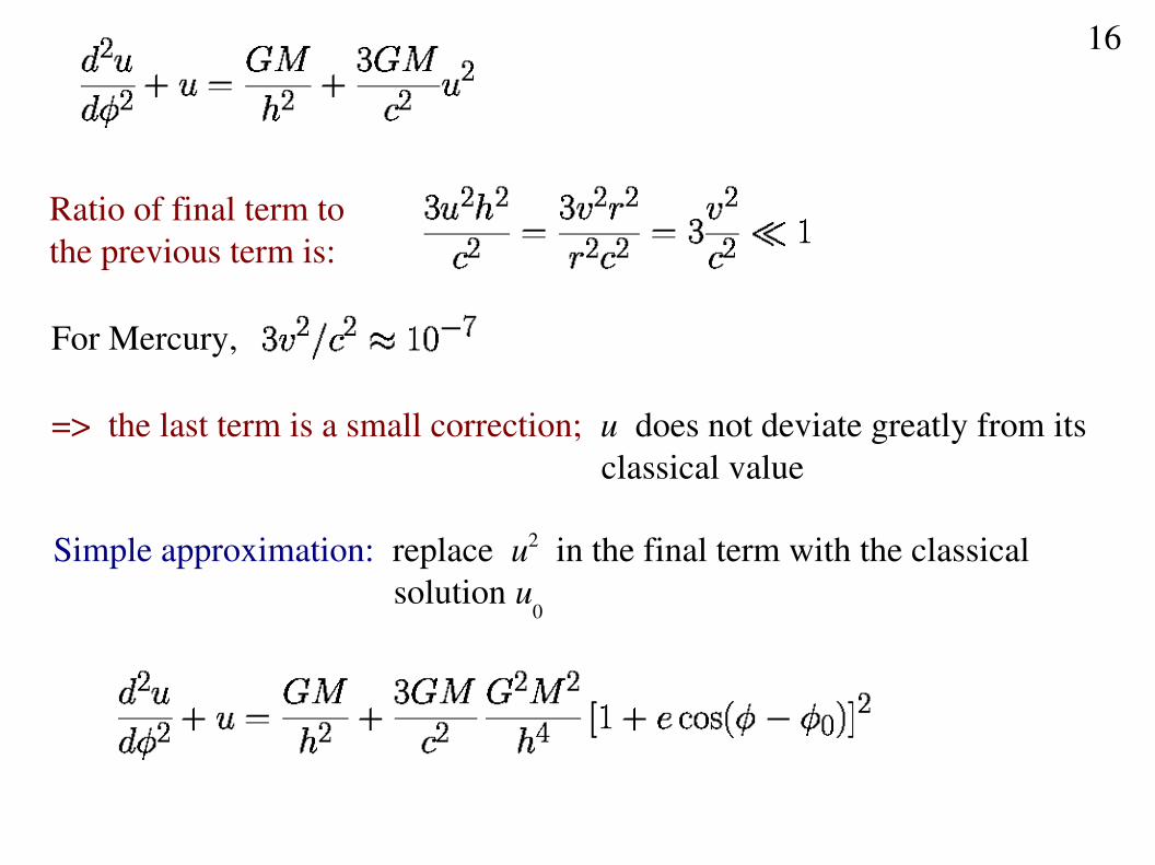
Ratio of final term to the previous term is:

For Mercury, 

=>  the last term is a small correction;  u  does not deviate greatly from its                                                               classical value

Simple approximation:  replace  u2  in the final term with the classical                                        solution u

0

16

Equation for a harmonic oscillator with a constant force and two oscillatory forcing terms.  

Of the three terms in the brackets:

1st :  a small correction to the size of the orbit  (a small change in the                                                                            constant forcing)

3rd :  imposes small oscillations on the orbit 

Both of the above effects are too small to observe.

2nd  term:  leads to a precession of the perihelion; too small to                  observe on a single orbit, but it accumulates over                  successive orbits, making it observable over long times.

17

Ignoring the 1st and 3rd terms in brackets:

Solution:

Last step took  sin x ≈ x   and   cos x ≈ 1.

Result is a precessing ellipse.

;

18

u

The argument of the cosine changes by 2 when  changes by:

Thus, perihelion precesses by angle per orbit.

The perihelion and aphelion distances are

The semimajor axis is

19

=>

Sun's mass M = 2 × 1033 g          G = 6.67 × 10­8  (cgs)

Mercury:  as = 0.39 AU = 5.8 × 1012 cm  ,   e = 0.206

                 orbital period = 0.24 yrs

=> =>  43''  per century

Observed perihelion shift is 574'' per century.  Almost of this is due to perturbations by the other planets.  The remainder is 43''per century, in exact agreement with GR.

20

2.  Deflection of Light Grazing the Sun

Lagrangian is the same as for massive particles, but we must adopt aparameter other than .  As for massive particles:

(Dot denotes differentiation wrt the affine parameter and subscript “p” denotes the photon case.)

ds2 = 0  =>

21

=>

=>

(RHS ≪ u  since  a ≪ r   =>   au ≪ 1)

In absence of RHS, solution is a straight line:

Use first approx for u in RHS:

22

Solution:

∞

∞

By symmetry, total deflection is 

23

Radius of Sun  =  6.96 × 1010 cm

=>   = 8.5 × 10­6 rad  =  1.75''

First verified (to within ≈20%) by Eddington in 1919.

Optical:  hard to improve precision much

Radio:  look at quasars; accuracy of 10­4

24

Gravitational lensing is now widely used in astronomy.(See Bartelmann 2010, Classical and Quantum Gravity, 27, 233001 for a review.)

In the simplest geometry, a point source of radiation lies directly behind aspherically symmetric massive body.

D

Robserverlens

ray from source

A gravitational lens with mass M is located a distance D from the observer.A ray located a perpendicular distance R from the center of the lens is bent 

through angle

If the lens radius < R, then the observer sees a luminous ring, called an “Einstein ring”.  In terms of M and D,

=>  the angular radius of the ring(“Einstein        radius”)

The impact parameter of the ray is also called the Einstein radius:

25

Very few Einstein rings have been observed, because it is highly unlikelythat the source will lie directly behind the lens and that the lens will be spherically symmetric.

In other geometries, lensing may still be observed on angular scales~

E :  ring arcs; multiple, distorted images of the source; magnification.  

Classified as “strong lensing” when there are multiple images and “weak lensing” when there is just a distortion of the one image.

The larger E , the more likely there are to be background sources that 

will be lensed.  Probability is ~ 10­6 when the lens is a star in the Galaxy.  Probability is higher for distant galaxies and ~ 1 for galaxy clusters observed with today's powerful telescopes (increase in M more than compensates for increase in D).

26

Lensing by stars in the Galaxy is called microlensing

E ≪ 1"  =>  lensing images are not resolved.  Instead, magnification as the 

lens star passes in front of the source star produces a characteristic light curve, with a timescale ~ weeks to months.

MACHO microlensing survey (Alcock et al. 2000, Astrophysical Journal, 542, 281) sought to infer the mass density of compact objects (low­mass stars, stellar remnants) in the Galaxy.  It observed 11.9 million stars over 5.7 years and found 13­17 events.  They concluded that 8% to 50% of the Galaxy's dark matter halo could be in the form of MACHOs (massive compact halo objects). So, MACHOs cannot account for all of the dark matter.

If a star has a planet located at a distance ≈ RE , then the planet can produce 

a detectable lensing signature.

27

The more recent EROS­2 survey (Tisserand et al. 2007, A&A, 469, 387) concludes that <8% of the dark matter halo could be in the form of MACHOs. 

(5.5 Earth mass planet at   2.6 AU separation; Beaulieu et al. 2006,         Nature, 439, 437)

To date, 34 microlensing planets have been discovered in 32 systems.(Jan 8, 2015)  (See the Extrasolar Planets Encyclopaedia at http://exoplanet.eu/catalog.php)

28

Lensing by galaxies and clusters of galaxies have multiple applications,including:

1.  Probing the mass distribution in the galaxy or cluster

2.  Estimating Hubble's constant, if the source luminosity is time variable            and multiple images are observed

3.  Use gravitational lensing as a telescope to get better info about the                 source

Lensing examples on the following pages are from Astronomy Picture of the Day  (http://antwrp.gsfc.nasa.gov/apod/).

29

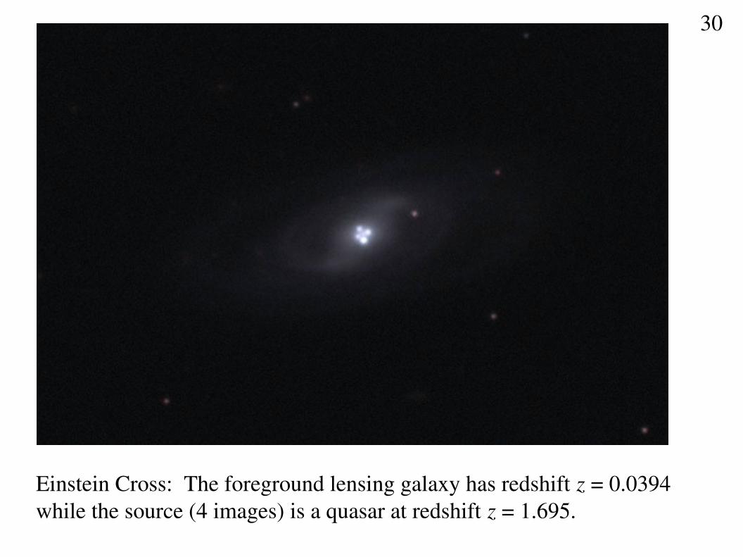
Einstein Cross:  The foreground lensing galaxy has redshift z = 0.0394 while the source (4 images) is a quasar at redshift z = 1.695.

30

Multiple images of a quasar and other sources; lens is clusterSDSS J1004+4112

31

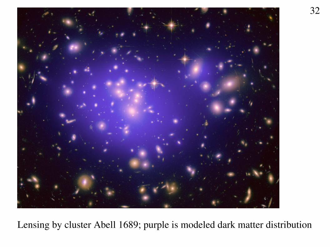
Lensing by cluster Abell 1689; purple is modeled dark matter distribution

32

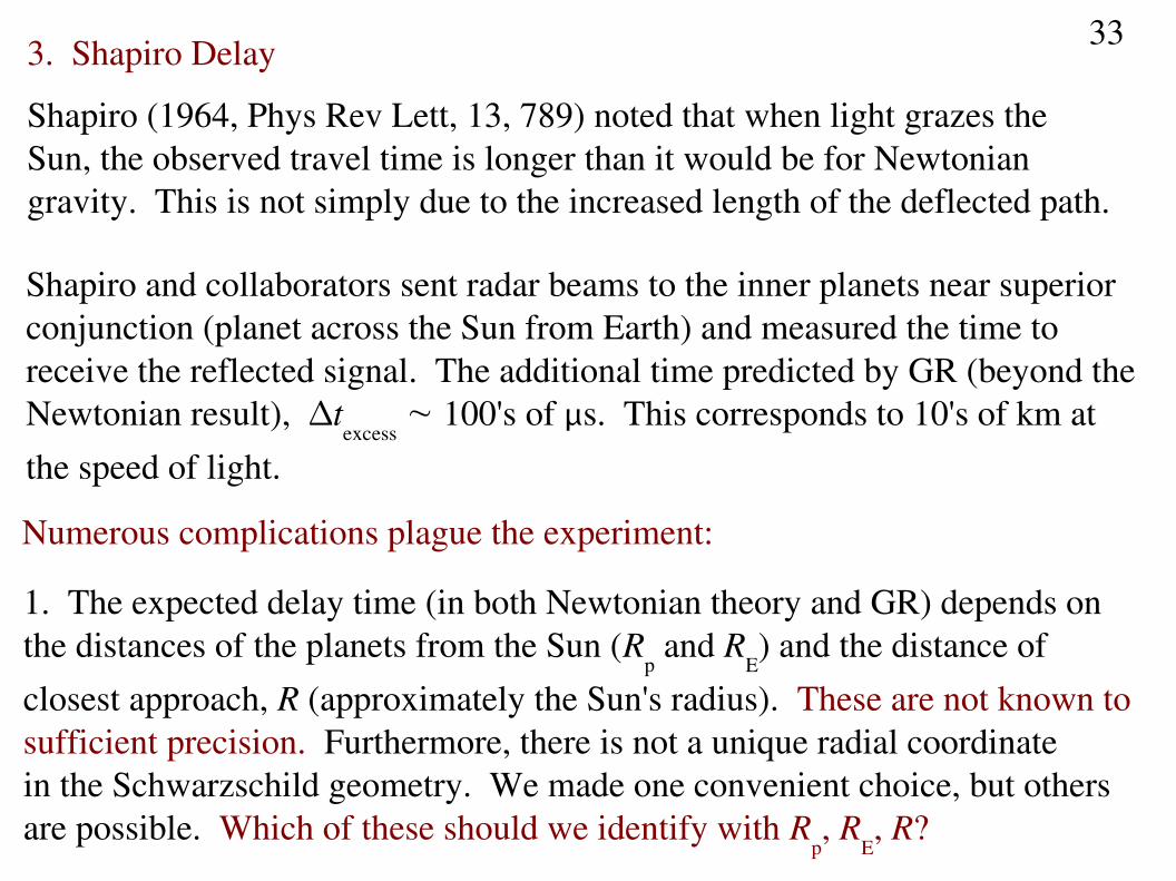
3.  Shapiro Delay

Shapiro (1964, Phys Rev Lett, 13, 789) noted that when light grazes the Sun, the observed travel time is longer than it would be for Newtoniangravity.  This is not simply due to the increased length of the deflected path.

Shapiro and collaborators sent radar beams to the inner planets near superior conjunction (planet across the Sun from Earth) and measured the time to receive the reflected signal.  The additional time predicted by GR (beyond the Newtonian result),  t

excess ~ 100's of s.  This corresponds to 10's of km at 

the speed of light.

Numerous complications plague the experiment:

1.  The expected delay time (in both Newtonian theory and GR) depends on the distances of the planets from the Sun (R

p and R

E) and the distance of

closest approach, R (approximately the Sun's radius).  These are not known tosufficient precision.  Furthermore, there is not a unique radial coordinatein the Schwarzschild geometry.  We made one convenient choice, but others are possible.  Which of these should we identify with R

p, R

E, R?

33

2.  The radar beam is refracted when it passes through the solar corona.  This has to be modeled.  (Use multiple radar frequencies.)

3.  Planet surfaces are rough.  So, there is a dispersion of delay timecomparable to  t

excess itself.  (Use satellites orbiting the planets with 

transponders that introduce a frequency shift in the radar beam, separating its signal from the planetary reflection.  Other complicated techniques can deal with the dispersion without the use of satellites.)

34

4.  The motion of the Earth and planet need to be taken into account, as well as effects from their own gravitational fields.

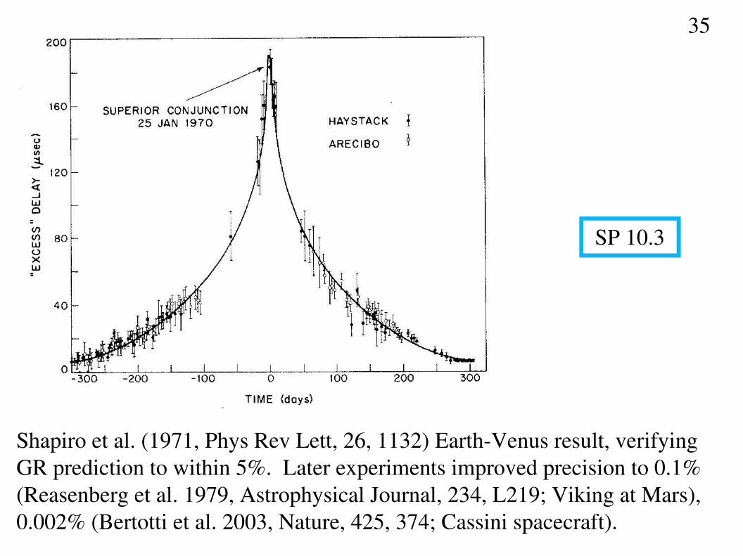
Strategy has been to measure delay times at numerous times (not justsuperior conjunction), producing a plot of excess radar delay time vs.time (i.e., vs. orientation of Earth­Sun­planet).  This curve can beextremely well fit using GR prediction and appropriate choices of R

p,  R

E, R.

Shapiro et al. (1971, Phys Rev Lett, 26, 1132) Earth­Venus result, verifying GR prediction to within 5%.  Later experiments improved precision to 0.1% (Reasenberg et al. 1979, Astrophysical Journal, 234, L219; Viking at Mars), 0.002% (Bertotti et al. 2003, Nature, 425, 374; Cassini spacecraft).

35

SP 10.3

Black Holes

Occur if the radius of the central mass < the Schwarzschild radius, a

As r  a,  grr  ∞ :  What's going on?

To find out, let's examine the behavior of particles on radial trajectories.

From the metric:

Recall (p. 11):

=>

36

Suppose particle is at rest when r = r0   =>

=>

=>

Exactly the same form as conservation of energy in Newtonian theory, but:   i) the dot denotes diff wrt , not t   ii) r is area (not radial) distance

Recall (p. 4):

as the particle falls radially inward.

37

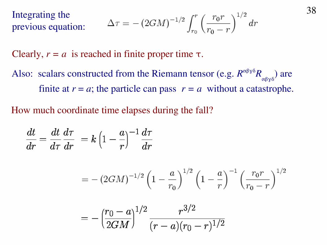
Integrating the previous equation:

Clearly, r = a  is reached in finite proper time .

Also:  scalars constructed from the Riemann tensor (e.g. RR

) are   

           finite at r = a; the particle can pass  r = a  without a catastrophe.

How much coordinate time elapses during the fall?

38

Coordinate time to fall from  r = r0  to  r = a +   is:

Given that  a +  < r   :   r > a   and   r0 – r < r

0

=>

 ∞   as     0

39

How does the fall look to a stationary observer at  r > a?Need to consider the paths of photons leaving the falling particleand arriving at the observer, i.e., radial null geodesics.

=>  0    as  r  a

=>  any photon that the observer sees must have been emitted when        the particle was still at  r > a

Outward­traveling light just sits still at  r = a  (not even any angularmotion).  Also, the frequency observed at  r > a  is zero; infinite redshift

40

The signs of the dt2 and dr2 terms change when r crosses a; r becomes the time coordinate!  There's only one direction to time;for r < a, that's the direction of decreasing r.  

=>  Any particle at  r < a  must fall inwards.  Same holds for photons       (since they must travel forward in time as seen by a particle)

=>  nothing can escape from  r < a.   

r = a  is known as the “event horizon”.

At  r = 0,  there is a true singularity, with scalars constructed from the Riemann tensor   ∞.

41