The search for gravitational waves from the coalescence of black hole binary systems in data from...

The Search for Gravitational Waves from the Coalescence of BlackHole Binary Systems in Data from the LIGO and Virgo Detectors

Or: A Dark Walk through a Random Forest

Thesis by

Kari Alison Hodge

In Partial Fulfillment of the Requirements

for the Degree of

Doctor of Philosophy

California Institute of Technology

Pasadena, California

2014

(Defended 12 May 2014)

ii

c© 2014

Kari Alison Hodge

All Rights Reserved

iii

To my parents

iv

Acknowledgments

First of all, I must thank my parents. You valued my education greatly and spent thousands of hours of

your lives driving me to another city so that my primary education would be one that challenged me, gave

me a problem-solving spirit, and encouraged creativity. Thank you for everything I learned from you directly

as well, especially the life skills that are not taught in school. Thank you for helping me with my school

projects, applying to colleges, and applying for financial aid. And lastly, thank you for encouraging me to not

drop out as an sophomore at USC. I never would have taken my first physics class the next semester, switched

my major, gotten a B.S. in physics, and certainly never would have found myself here today.

Secondly, I thank Alan Weinstein. After meeting with you as a prospective, I was infected with your

enthusiasm and joined the LIGO data analysis group. Thank you for your guidance and your seemingly

infinite knowledge of all aspects of LIGO. Thank you for believing in me even when you had to explain

things that I probably should have known already. Thank you for your kindness and understanding of my

need to do theater, and for coming to all of my performances. Thank you meeting with me weekly to discuss

my thesis, even when it became apparent that I was going to be releasing a lot of stress through my eyeballs

during these meetings. I could not have picked a better advisor. Thank you for taking me on as a student.

Thank you to my candidacy/defense committee — Yanbei Chen, Ken Libbrecht, and Sunil Golwala. And,

of course, thank you to LIGO lab for funding me, allowing me to learn so much, and letting me travel to many

conferences. Special thanks to everyone in the CBC and Detchar groups for embracing me and my work. A

huge thank you to all the system administrators for the clusters (I think I used every single one!) — this thesis

would have been impossible without you.

There are so many other people I want to thank, I cannot even conceive of putting them in some order.

To the physics graduate students in the entering class of 2007, especially Milivoje Lukic, Evan O’Connor,

Brian Willet, Laura Book, Mhair Orchanian, Paula Popescu, and Kevin Engel — thank you for teaching

me more physics than I could have learned alone. I truly enjoyed our time in the library doing homework

problems and all the dinners out and boardgames. Extra thanks goes to Richard Norte and Jeff Kaplan who

were my study partners and formidable Wii tennis opponents during the epic prep for our qualifying exams.

Thank you for letting me into your home and letting me make espresso and chill on your balcony whenever I

wanted. And Norte — thank you for always being up for an adventure and, lately, writing your own thesis in

the library next to me — it really kept me on task. And thank you Henry Kozachkov for being a good friend

v

all these years.

And let me thank my fellow LIGO graduate students at Caltech. Stephen Privitera — sorry I got you

involved in LIGO in the first place (just kidding, I know you love it) and thank you for helping me with

the high-mass search and for letting me plan that crazy train adventure through Germany, Belgium, and

the Netherlands (I’m sorry I almost got you stabbed). Leo Singer — your passion for astrophysics is truly

inspiring. Jenne Driggers — thank you for being a super cool experimentalist and organizing that trip to the

National Ignition Facility. David Yeaton-Massey — thank you for not running me over in the stairwell (I

can’t believe I’m making it through all these years in Bridge unscathed!). Eric Quintero — thanks for riding

bikes with me in Boston. Drew Keppel — thank you for your help and for being such a role model. Lisa

Goggin and Pinkesh Patel — thank you for showing me that finishing was possible.

I cannot forget to thank the other LIGO colleagues and collaborators I have had the pleasure of working

with. Chad Hannah and Kipp Cannon — thank you for all your help with python and sqlite and for helping

me install lalsuite countless times; you really helped launch my projects into action and taught me how to

“fish”. Tom Dent — thank you for being my partner in crime for the high-mass search and for making me

think twice about several aspects of my own research; I really learned a lot from you. Collin Capano —

thank you for all your pipedown help along the way and especially for writing dbinjfind, which was integral

in the successful implementation of my random forest of bagged decison trees. Andrew Lundgren, Marco

Cavaglia, and Duncan MacLeod — thank you for all your help with data quality and veto definer files. Jacob

Slutsky — thank you for hanging out with me when I was a SciMon at Livingston and adventuring with me

in other countries (especially because I know my lack of planning is not your style). And special thanks to

all my AuxMVC collaborators — Ruslan Vaulin, Lindy Blackburn, Reed Essick, John J Oh, SangHoon Oh,

Rahul Biswas, Kyungmin Kim, Young-Min Kim, EOL Bigot, Chang-Hwan Lee, Edwin Son, Xiaoge Wang,

Junwei Cao, and Erik Katsavounidis. And thank you Sarah Caudill and Paul Baker for getting my crazy

random forest of bagged decision trees into a published search; it was great working with you, and I learned

a lot. Tristan Ursell and Colorado Reed — thank you for being my SURF students; it was a very educational

experience for me too. And thank you to Rana Adhikari for ruling the bodega with an iron fist, such that 2nd

floor Bridge has the best coffee on campus.

Thank you to everyone who helped me “Dance my PhD” — Anne Grauso, Morgan Gillio, Jared Frank,

Samantha Jacober, Crystal Dilworth, David Brown, Dagny Fleischman, Willie Stanphill, Amit Lakhanpal,

Doug Smith, Steve Collins, Klavdia Zemlianova, Yulan Lin, and Chandrea Patterson. And especially Alan

Weinstein for your appearance as an electromagnetic glitch and for leading us in the LIGO dance at the end.

And of course, thank you to everyone in the LIGO-Virgo Collaboration who went dancing with me during

our (inter)national conferences. It was such a joy to boogie with you all — especially Brennan Hughey, Chris

Pankow, Lucia Santamaria, Nick Fotopoulos, Melissa Frei, Larry Price, and Jamie Rollins.

Thank you to my theater family at Caltech. You truly kept me happy and sane. Brian Brophy, Benjamin

Sveinbjornsson, Crystal Dilworth, Meg Rosenberg, Miranda Stewart, Dave Seal, Christine Kennedy, and

vi

Ann Lindsey — thank you! And most of all, Amit Lakhanpal — thank you for all our library time and for

becoming one of my best and truest friends.

And thank you to my Orlando House/Phageling family for making me feel at home when I am with you.

Thank you to all my office mates through the years — Aidan Brooks, Matt Abernathy, Gabriele Vajente,

Steven Privitera, Lucia Santamaria, Ajith Parameswaran, Peter Kalmus, Larry Price, Anand Sengupta, Steve

Fairhurst, Lisa Goggin, Drew Keppel, and Diego Fazi. Thank you for all your great company, for the good

conversation, and for putting up with my messy desk.

Lynnie Hedvig — thank you for always revitalizing me whenever we get to see each other. You’ll always

be my first “my”. Elizabeth Forest — thank you for your beautiful mind and spirit. To be seen the way you

see me, from a person as good as you, really gives me confidence. Nicole Pyburn (Valenzuela) — thank you

for your unconditional love. Seren Rain Sehota — thank you for being a great roommate and for giving me

word count motivations as I was embarking on this thesis. Shaun Maguire — thank you for being above-and-

beyond supportive and always making the time to talk, despite how insanely busy you are. You have helped

me in so many ways. Joshy Roche (and Frankie Staniszewski) — thank you for recognizing that this physics

thing was totally right for me and for getting me pumped about it. Thank you for supporting me in those early

years. Samantha Jacober — thank you for always making me feel at home, even before we lived together.

Matt Gangi — thank you for your continued interest in my science, it is definitely re-energizing to have your

perspective. Leah Yananton, Dawn Batson, Zorina Chen, Victoria Asher, Jenae Wilkens, Sara Drakely, Dieu

Ha, Vi Ha, and Drew Denny — thank you for being amazing women and true sources of inspiration in my

life.

Thank you so, so much to everyone who came to my defense — it was so meaningful to have all of your

love and support. And thank you for clapping even though you weren’t supposed to. You made it a memory

I will always treasure.

vii

Abstract

The LIGO and Virgo gravitational-wave observatories are complex and extremely sensitive strain detec-

tors that can be used to search for a wide variety of gravitational waves from astrophysical and cosmological

sources. In this thesis, I motivate the search for the gravitational wave signals from coalescing black hole

binary systems with total mass between 25 and 100 M�. The mechanisms for formation of such systems

are not well-understood, and we do not have many observational constraints on the parameters that guide the

formation scenarios. Detection of gravitational waves from such systems — or, in the absence of detection,

the tightening of upper limits on the rate of such coalescences — will provide valuable information that can

inform the astrophysics of the formation of these systems. I review the search for these systems and place

upper limits on the rate of black hole binary coalescences with total mass between 25 and 100 M�. I then

show how the sensitivity of this search can be improved by up to 40% by the the application of the multivari-

ate statistical classifier known as a random forest of bagged decision trees to more effectively discriminate

between signal and non-Gaussian instrumental noise. I also discuss the use of this classifier in the search for

the ringdown signal from the merger of two black holes with total mass between 50 and 450 M� and present

upper limits. I also apply multivariate statistical classifiers to the problem of quantifying the non-Gaussianity

of LIGO data. Despite these improvements, no gravitational-wave signals have been detected in LIGO data

so far. However, the use of multivariate statistical classification can significantly improve the sensitivity of

the Advanced LIGO detectors to such signals.

viii

Preface

The work presented in this thesis was carried out within the LIGO Scientific Collaboration (LSC). The

methods and results presented here are under review and are potentially subject to change. The opinions ex-

pressed here are those of the author and not necessarily those of the LSC. The author gratefully acknowledges

the support of the United States National Science Foundation for the construction and operation of the LIGO

Laboratory, which provided support for this work.

ix

Contents

Acknowledgments iv

Abstract vii

Preface viii

1 The search for gravitational waves from the coalescence of black hole binary systems 1

1.1 The motivation for the search for gravitational waves from black hole binary systems . . . . 2

1.2 Issues associated with the search for high-mass compact binary coalescence (CBC)s . . . . . 3

1.3 Mitigating the effect of glitches in the search for high-mass CBCs . . . . . . . . . . . . . . 3

2 The physics and astrophysics of gravitational waves from compact binary coalescences with

total mass of 25 − 100 M� 6

2.1 Astrophysics of compact binaries with two black holes or one black hole and one neutron star 6

2.1.1 Isolated binary evolution . . . . . . . . . . . . . . . . . . . . . . . . . . . . . . . . 7

2.1.2 Population synthesis . . . . . . . . . . . . . . . . . . . . . . . . . . . . . . . . . . 9

2.1.3 Dynamical formation scenarios . . . . . . . . . . . . . . . . . . . . . . . . . . . . 10

2.1.3.1 Globular clusters . . . . . . . . . . . . . . . . . . . . . . . . . . . . . . . 11

2.1.3.2 Galactic nuclei . . . . . . . . . . . . . . . . . . . . . . . . . . . . . . . . 12

2.1.4 Observational evidence from low-metallicity galaxies . . . . . . . . . . . . . . . . . 12

2.2 The physics of gravitational waves from compact binary coalescences . . . . . . . . . . . . 13

2.2.1 The mathematical formulation of gravitational waves . . . . . . . . . . . . . . . . . 13

2.2.1.1 Effective-one-body + numerical relativity (EOBNR) waveforms . . . . . . 17

2.2.1.2 Phenomenological waveforms including spin . . . . . . . . . . . . . . . . 25

2.2.2 The sensitivity of the detectors to compact binary coalescences . . . . . . . . . . . . 29

3 Ground-based interferometric gravitational wave (GW) detection 32

3.1 The operating principles of ground-based interferometric GW detectors . . . . . . . . . . . 34

3.1.1 Subsystems of the LIGO interferometers . . . . . . . . . . . . . . . . . . . . . . . 36

3.1.2 Data channels . . . . . . . . . . . . . . . . . . . . . . . . . . . . . . . . . . . . . . 39

x

3.2 Antenna response of detector to GW signals . . . . . . . . . . . . . . . . . . . . . . . . . . 40

3.3 Calibration . . . . . . . . . . . . . . . . . . . . . . . . . . . . . . . . . . . . . . . . . . . 44

3.3.1 Hardware injections . . . . . . . . . . . . . . . . . . . . . . . . . . . . . . . . . . 49

3.4 LIGO and Virgo detectors’ noise . . . . . . . . . . . . . . . . . . . . . . . . . . . . . . . . 50

3.4.1 Gaussian versus non-Gaussian noise . . . . . . . . . . . . . . . . . . . . . . . . . . 52

4 Glitches, their effect on data quality, and the need for vetoes 55

4.1 Glitches and glitch-finding algorithms . . . . . . . . . . . . . . . . . . . . . . . . . . . . . 55

4.1.1 KleineWelle as a glitch-finding algorithm . . . . . . . . . . . . . . . . . . . . . . . 56

4.1.2 Omega as a glitch-finding algorithm . . . . . . . . . . . . . . . . . . . . . . . . . . 58

4.1.3 Detector characterization and glitch examples . . . . . . . . . . . . . . . . . . . . . 60

4.1.3.1 Grid glitches . . . . . . . . . . . . . . . . . . . . . . . . . . . . . . . . . 61

4.1.3.2 Flip glitches . . . . . . . . . . . . . . . . . . . . . . . . . . . . . . . . . 61

4.1.3.3 Upconversion noise . . . . . . . . . . . . . . . . . . . . . . . . . . . . . 63

4.1.3.4 Spike Glitches . . . . . . . . . . . . . . . . . . . . . . . . . . . . . . . . 64

4.2 The need for vetoes . . . . . . . . . . . . . . . . . . . . . . . . . . . . . . . . . . . . . . . 64

4.2.1 Vetoes/flags for the high-mass search . . . . . . . . . . . . . . . . . . . . . . . . . 66

4.2.1.1 Data-quality flags created from the data monitoring tools (DMT) . . . . . 68

4.2.1.2 Data-quality flags created by persons in the detector characterization group

(DCH) . . . . . . . . . . . . . . . . . . . . . . . . . . . . . . . . . . . . 69

4.2.1.3 Used percentage vetoes (UPV) . . . . . . . . . . . . . . . . . . . . . . . 70

4.2.1.4 Bilinear coupling vetoes (BCV) . . . . . . . . . . . . . . . . . . . . . . . 71

4.2.1.5 Veto safety . . . . . . . . . . . . . . . . . . . . . . . . . . . . . . . . . . 72

5 Review of Multivariate Statistical Classification/Machine Learning 73

5.1 Artificial neural networks . . . . . . . . . . . . . . . . . . . . . . . . . . . . . . . . . . . . 74

5.1.1 Multi-layer perceptron model . . . . . . . . . . . . . . . . . . . . . . . . . . . . . 75

5.1.1.1 Resilient back-propagation . . . . . . . . . . . . . . . . . . . . . . . . . 76

5.2 Support vector machines . . . . . . . . . . . . . . . . . . . . . . . . . . . . . . . . . . . . 76

5.2.1 LibSVM . . . . . . . . . . . . . . . . . . . . . . . . . . . . . . . . . . . . . . . . 77

5.3 Random forest of bagged decision trees . . . . . . . . . . . . . . . . . . . . . . . . . . . . 78

5.3.1 The binary tree . . . . . . . . . . . . . . . . . . . . . . . . . . . . . . . . . . . . . 78

5.3.2 Bagging and random forest technology . . . . . . . . . . . . . . . . . . . . . . . . 80

5.3.2.1 StatPatternRecognition . . . . . . . . . . . . . . . . . . . . . . . . . . . 81

6 Multivariate statistical classifiers for data quality and detector characterization 83

6.1 Data preparation for use with the KleineWelle event-based method . . . . . . . . . . . . . . 84

xi

6.2 General formulation of the detection problem . . . . . . . . . . . . . . . . . . . . . . . . . 85

6.2.1 Tuning the machine learning algorithms (ANN, SVM, RFBDT) . . . . . . . . . . . 87

6.2.2 Ordered veto list as a benchmark . . . . . . . . . . . . . . . . . . . . . . . . . . . . 88

6.2.3 Testing the algorithms’ robustness at finding glitches while keeping low dead-time . 89

6.2.3.1 Evaluating and comparing classifiers’ performance . . . . . . . . . . . . . 95

6.2.3.2 Methods for combining classifiers . . . . . . . . . . . . . . . . . . . . . . 98

6.3 Conclusions and additional benefits of this approach . . . . . . . . . . . . . . . . . . . . . . 102

6.3.1 Future work . . . . . . . . . . . . . . . . . . . . . . . . . . . . . . . . . . . . . . . 104

7 Data analysis methods in the search for black hole binary systems 106

7.1 The inputs to the search . . . . . . . . . . . . . . . . . . . . . . . . . . . . . . . . . . . . . 107

7.2 The signals we are looking for . . . . . . . . . . . . . . . . . . . . . . . . . . . . . . . . . 108

7.3 The two-stage search pipeline for an all-sky all-time search for compact binary coalescences

— ihope . . . . . . . . . . . . . . . . . . . . . . . . . . . . . . . . . . . . . . . . . . . . . 111

7.3.1 Data preparation . . . . . . . . . . . . . . . . . . . . . . . . . . . . . . . . . . . . 113

7.3.2 Template bank generation . . . . . . . . . . . . . . . . . . . . . . . . . . . . . . . 114

7.3.3 The matched-filter . . . . . . . . . . . . . . . . . . . . . . . . . . . . . . . . . . . 116

7.3.4 Coincidence between detectors . . . . . . . . . . . . . . . . . . . . . . . . . . . . . 118

7.3.5 The second stage of template bank creation, matched-filter, and coincidence . . . . . 119

7.3.6 A χ2 test for the consistency of the frequency content of the data with the waveform

template . . . . . . . . . . . . . . . . . . . . . . . . . . . . . . . . . . . . . . . . . 120

7.3.7 A final clustering stage . . . . . . . . . . . . . . . . . . . . . . . . . . . . . . . . . 121

7.3.8 The candidate gravitational wave events . . . . . . . . . . . . . . . . . . . . . . . . 121

7.4 The estimation of the background — accidental coincidences between detectors (timeslides) 123

7.5 The injection of simulated signals to test our efficiency and make astrophysical statements . 123

7.6 A ranking statistic for candidate GW events . . . . . . . . . . . . . . . . . . . . . . . . . . 131

7.7 False alarm rate calculations . . . . . . . . . . . . . . . . . . . . . . . . . . . . . . . . . . 135

7.8 The loudest event statistic and sensitivity . . . . . . . . . . . . . . . . . . . . . . . . . . . . 136

7.8.1 Upper limit calculation for the rate of high-mass binary mergers . . . . . . . . . . . 137

7.9 Blind Analysis . . . . . . . . . . . . . . . . . . . . . . . . . . . . . . . . . . . . . . . . . 139

7.10 Criteria for detection . . . . . . . . . . . . . . . . . . . . . . . . . . . . . . . . . . . . . . 139

7.11 Changes that will be made to this pipeline for Advanced LIGO searches . . . . . . . . . . . 141

8 Results of searches for high mass binary signals 142

8.1 Efficiency at finding simulated gravitational wave signals . . . . . . . . . . . . . . . . . . . 142

8.2 Null result and search sensitivity/upper limit on astrophysical events . . . . . . . . . . . . . 143

8.3 Improvements to the analysis using multivariate statistical classifiers . . . . . . . . . . . . . 151

xii

8.3.1 Random forest of bagged decision trees as a classifier trained on signal-based infor-

mation . . . . . . . . . . . . . . . . . . . . . . . . . . . . . . . . . . . . . . . . . 151

8.3.1.1 Handling the different qualities of the different detector combinations . . . 151

8.3.1.2 Choosing good examples of signal and background for our training sets . . 152

8.3.1.3 Round-robin procedure for training and evaluating the performance of the

classifier . . . . . . . . . . . . . . . . . . . . . . . . . . . . . . . . . . . 153

8.3.1.4 Inputs to the classifier . . . . . . . . . . . . . . . . . . . . . . . . . . . . 153

8.3.1.5 Turning the classifier output into a detection statistic . . . . . . . . . . . . 164

8.3.1.6 Efficiency and sensitivity comparisons between the RFBDT analysis and

the standard analysis . . . . . . . . . . . . . . . . . . . . . . . . . . . . . 164

8.3.1.7 . . . . . . . . . . . . . . . . . . . . . . . . . . . . . . 166

8.3.1.8 Additional information from the multivariate statistical classifier . . . . . 177

8.3.2 Conclusions from using a multivariate statistical classifier to calculate the rank of

events in the high-mass search . . . . . . . . . . . . . . . . . . . . . . . . . . . . . 177

8.3.2.1 Future work . . . . . . . . . . . . . . . . . . . . . . . . . . . . . . . . . 177

9 Application of RFBDTs to the search for black hole ringdown signals 180

9.1 Multivariate statistical classifiers in ringdown search . . . . . . . . . . . . . . . . . . . . . 181

9.1.1 Efficiency and upper limits on the rates of astrophysical sources . . . . . . . . . . . 182

9.1.2 Conclusions from this search for ringdown signals . . . . . . . . . . . . . . . . . . 184

10 Summary of this work 185

10.1 Future work . . . . . . . . . . . . . . . . . . . . . . . . . . . . . . . . . . . . . . . . . . . 186

10.2 Long term outlook for the field . . . . . . . . . . . . . . . . . . . . . . . . . . . . . . . . . 186

Bibliography 188

xiii

List of Figures

1.1 A cartoon plot representing the overlap of signal and background in different situations. Blue:

Background triggers due to Gaussian noise, picked up by a search with low-mass templates.

Cyan: Background triggers due to Gaussian noise, picked up by a search with low-mass and

high-mass templates. Black: Background triggers due to Gaussian and non-Gaussian noise,

picked up by a search with low-mass templates. Green: Background triggers due to Gaussian

and non-Gaussian noise, picked up by a search with low-mass and high-mass templates. Red:

Theoretical signal distribution for low-mass astrophysical signals. Magenta: Theoretical signal

distribution for low-mass and high-mass astrophysical signals, assuming there are an equal

number of each. . . . . . . . . . . . . . . . . . . . . . . . . . . . . . . . . . . . . . . . . . 4

2.1 The mass distributions of various kinds of single BHs at 11 Myr based on simulations using

Reference [1]’s standard model (A). The dotted line indicates BHs evolved from primordial

single stars; the dashed line shows single BHs from disrupted binaries; and the solid line shows

single BHs that are remnants of merged binaries. The bin width is 2.0 M�and the counts are

normalized to the total number of BHs [1]. . . . . . . . . . . . . . . . . . . . . . . . . . . . 7

2.2 Histograms of number versus chirp mass for 4 different Population Synthesis scenarios [2].

The top two panels are for simulations of category A, in which progenitor stars are allowed to

remain distinct and can continue evolving into a double compact object even if the donor star is

evolving through the Hertzsprung gap during the common envelope phase; the bottom two are

for category B, in which the progenitor stars merge if the common envelope phase is initiated

by a Herzsprung gap star. Note that for both A and B, both the number of, and the maximum

chirp mass (which, as we will see in Section 2.2.1, is the relevant combination of component

masses used for describing CBCs) increase for the systems with 10 percent solar metallicity

(second and fourth panels) [2]. . . . . . . . . . . . . . . . . . . . . . . . . . . . . . . . . . 10

xiv

2.3 A comparison of two numerical simulations of BH pair formation in globular clusters. The left

panel (a) shows the least efficient (out of 46 simulations) cluster, in terms of producing large

BHs and BH+BH binaries. The right panel (b) does not reach equipartition (when the rate of

BH interactions with other stars in the cluster is less than or equal to the rate of BHs with other

BHs) before a Hubble time; therefore, there are many more BHs in the cluster — allowing the

formation of many more binaries. The x-axis is time since the beginning of the simulation (11

Myr after the Big Bang) [3]. . . . . . . . . . . . . . . . . . . . . . . . . . . . . . . . . . . . 11

2.4 The effect of gravitational waves on a circle of particles in a plane perpendicular to the direction

of propagation. The left panel shows a purely plus-polarized GW. During a full period of the

GW, the particles go from circle to horizontal ellipse to circle to vertical ellipse back to circle.

The right panel shows a purely cross-polarized GW. . . . . . . . . . . . . . . . . . . . . . . 16

2.5 A screenshot from a Caltech-Cornell numerical relativity (NR) simulation of two equal-mass

nonspinning black holes. Visit for the full movie and more animated simulations. . . . . . . . 17

2.6 A screenshot, at merger, from a NR simulation of two black holes with a mass ratio of 6:1

and non-aligned spins of .91 and .3, respectively. Note the amplitude and phase modulation,

which is due to the precession of the orbital plane resulting from the spin-orbit coupling of the

non-aligned spins. Visit http://www.black-holes.org/explore2.html for the full movie and more

animated simulations. . . . . . . . . . . . . . . . . . . . . . . . . . . . . . . . . . . . . . . 18

2.7 Time-domain waveforms for a 12.5 M�+ 12.5 M�system. . . . . . . . . . . . . . . . . . . 19

2.8 Time-domain waveforms for a 45 M�+ 45 M�system. . . . . . . . . . . . . . . . . . . . . 20

2.9 An EOBNRv2 time-domain waveform for a 1 M�+ 24 M�system. Note that the merger and

ringdown are present even though not visible due to the scale of the plot. The IMRPhenomB

waveform is not plotted, as it is not valid for this mass ratio. . . . . . . . . . . . . . . . . . . 21

2.10 An EOBNRv2 time-domain waveform for a 1 M�+ 99 M�system. The IMRPhenomB wave-

form is not plotted, as it is not valid for this mass ratio. . . . . . . . . . . . . . . . . . . . . . 22

2.11 Waveforms for a 12.5 M�+ 12.5 M� system in the frequency domain, compared to the mode

of H1’s noise amplitude spectral density during S6 [4]. The EOBNR waveform was originally

in the time domain, and was fast Fourier transformed into the frequency domain, resulting in

non-physical wiggles. The green dashed curve indicates the frequency journey of an inspiral-

only waveform, whose amplitude has been set by the IMRPhenomB waveform. Merger is short

and has an undefined duration. The Fourier transform of a ringdown is the imaginary part of a

Lorentzian, and can be seen in this plot beginning when the blue or red curve deviates (has a

less steep slope) from the green dashed curve and continuing through the steeper negative slope

towards the right of the plot, remembering that the wiggles on the blue curve are non-physical. 23

xv

2.12 Waveforms for a 50 M�+ 50 M� system in the frequency domain, compared to the mode of

H1’s noise amplitude spectral density during S6 [4]. The EOBNR waveform was originally in

the time domain, and was fast Fourier transformed into the frequency domain, resulting in non-

physical wiggles throughout the waveform, since the waveform has a finite duration. The green

dashed curve indicates the frequency journey of an inspiral-only waveform, whose amplitude

has been set by the IMRPhenomB waveform. Merger is short and has an undefined duration.

The Fourier transform of a ringdown is the imaginary part of a Lorentzian, and can be seen in

this plot beginning when the blue or red curve deviates (has a less steep slope) from the green

dashed curve and continuing through the steeper negative slope towards the right of the plot,

remembering that the wiggles on the blue curve are non-physical. . . . . . . . . . . . . . . . 24

2.13 Time-domain waveforms for a 12.5 M�+ 12.5 M�system. Blue: neither black hole is spin-

ning. Red: dimensionless spins are aligned but unequal in magnitude (χ1 = 0.85, χ2 = 0.5),

giving a combined spin parameter of χ = 0.675. . . . . . . . . . . . . . . . . . . . . . . . . 26

2.14 Time-domain waveforms for a 12.5 M�+ 12.5 M�system. Blue: neither black hole is spin-

ning. Red: dimensionless spins are anti-aligned, and equal in magnitude (χ1,2 = 0.5). The red

and blue curves lie atop one another, as is expected — the combined spin parameter χ = 0 for

both systems. . . . . . . . . . . . . . . . . . . . . . . . . . . . . . . . . . . . . . . . . . . . 27

2.15 Time-domain waveforms for a 10 M�+ 40 M�system. Blue: neither black hole is spinning

(χ = 0). Red: dimensionless spins are aligned and equal in magnitude, with χ = 0.5. . . . . 27

2.16 Time-domain waveforms for a 10M�+ 40M�system. Both waveforms are from systems with

component black holes having anti-aligned spins. Blue: a 10 M� black hole with χ1 = −0.5

with a 40 M� black hole with χ2 = 0.5, giving a combined spin parameter of χ = 0.3. Red: a

10M� black hole with χ1 = 0.5 with a 40M� black hole with χ2 = −0.5, giving a combined

spin parameter of χ = −0.3. . . . . . . . . . . . . . . . . . . . . . . . . . . . . . . . . . . 28

2.17 Representative curves for the strain amplitude sensitivity for LIGO Livingston (L1), in solid

red, and LIGO Hanford (H1), in green, during S6 as compared to S5 (dotted lines). Note that

S6 performance exceeded the Science Requirements Document (SRD) for Initial LIGO, due to

enhancements made between S5 and S6. The distances in the legend are the horizon distance

for an optimally oriented NS+NS inspiral. Image courtesy of John Zweizig. . . . . . . . . . 30

2.18 Representative curves for the strain amplitude sensitivity for Virgo during Virgo science run

(VSR) 1, 2, and 3 [5]. Note that VSR1 was during S5, while VSR2 and VSR3 were during S6. 31

2.19 Horizon distances for non-spinning equal-mass inspiral-merger-ringdown (IMR) signals in the

LIGO and Virgo detectors, using EOBNRv2 waveforms, which are explained in Section 2.2.1.1

as the signal model, averaged over periods of data when the detector sensitivities were near op-

timal for S6 and VSR2/3, respectively [4]. Note that above 100M�, the horizon distance drops

abruptly, as the number of cycles in the detectors’ sensitive bands go to zero (see Table 2.2). . 31

xvi

3.1 An arial view of LIGO Livingston (L1) showing the full y-arm, part of the x-arm and the

exterior building around the control room and laser and vacuum equipment area. Image taken

from www.ligo.org. . . . . . . . . . . . . . . . . . . . . . . . . . . . . . . . . . . . . . . . 33

3.2 An arial view of LIGO Hanford (H1 and H2) showing the full y-arm, part of the x-arm and the

exterior building around the control room and laser and vacuum equipment area. Image taken

from www.ligo.org. . . . . . . . . . . . . . . . . . . . . . . . . . . . . . . . . . . . . . . . 33

3.3 A basic illustration of a LIGO detector and its main components during S6 [6]. . . . . . . . . 35

3.4 The range (See Equation (2.25) to which the LIGO detectors are sensitive to a binary neutron

star inspiral signal, shown to illustrate the changing sensitivity as various hardware or software

upgrades are made throughout the course of the run [6]. . . . . . . . . . . . . . . . . . . . . 36

3.5 An illustration of the input optics subsystem for LIGO during S6 (enhanced LIGO). The

electro-optic modulator produces the RF sidebands that are used by other subsystems; this

is the last component that is outside the vacuum. The mode cleaner suppresses laser light that

is not in the TEM00 mode, provides frequency stabilization, and passively reduces beam jitter

above 10 Hz. The Faraday isolator prevents back-propagation of the laser and provides access

to the symmetric port beam for length and alignment-sensing [7]. . . . . . . . . . . . . . . . 39

3.6 An illustration of the angular-sensing and control subsystem for LIGO during S6 (enhanced

LIGO). The QPDs (quadrant photodiodes) sense the alignment of the light transmitted to the

ETMs (end test masses). The WFSs (wavefront sensors) sense the angular alignment of the

input beams with respect to their resonant cavity modes. The camera senses the beam position

incident on the BS (beam splitter). The positions of the ETMs, BS, ITMs (input test masses),

RM (recycling mirror), and MMTs (mode matching telescopes) are adjusted with OSEMs via

a servo using the information from the QPDs and WFSs. [8] . . . . . . . . . . . . . . . . . . 40

3.7 A diagram depicting the locations of physical environmental sensor locations at L1. Figure

courtesy of Annamaria Effler. . . . . . . . . . . . . . . . . . . . . . . . . . . . . . . . . . . 42

3.8 A representation of the seismic isolation stack for one of the suspended optics. Inside the

dashed line is the vacuum system. The isolation stack provides passive isolation and the sensor

and actuator are used to provide active seismic isolation in the x- and y-directions [9]. . . . . 43

3.9 A representation of the output mode cleaner optical setup [10]. . . . . . . . . . . . . . . . . 43

3.10 A diagram depicting the locations of various optical components and the auxiliary channels

recording information from/about them. Figure courtesy of Jeff Kissel. . . . . . . . . . . . . 44

xvii

3.11 The relevant angles for the calculation of the strain seen by an interferometric GW detector.

The x’-y’-z’ frame is that of the detector, the x-y-z frame is that of the source, and the x”-y”-z”

frame is that of the GWs. ψ is the polarization angle. The z-axis is defined by aligning it with

the orbital angular momentum of the binary system. The z”-axis is defined by the direction

from the source to the detector; the x”- and y”-axes are defined by the stretching and squeezing

directions of h+ in the GW frame (see Figure 2.4). The x’- and y’-axes are defined by the arms

of the detector; we then use the right hand rule to define the z’-axis [11]. . . . . . . . . . . . 45

3.12 The root mean square antenna pattern of a LIGO detector whose x- and y-arms are represented

by the black bars to circularly polarized GWs [12]. . . . . . . . . . . . . . . . . . . . . . . . 46

3.13 The control loop for LIGO interferometers. ∆Lext is the motion of the mirrors caused by GWs

or a local disturbance, γ(t)C(f) is the length-sensing function, eD is digital error signal, D(f)

is the set of digital filters on eD in order to feed it into is the actuation function A(f) that

calculates the ∆LA in an attempt to cancel the ∆Lext. . . . . . . . . . . . . . . . . . . . . . 46

3.14 A whitened time-frequency spectrogram illustrating a GW signal from a 18.901 + 15.910

M� system, at a distance of 19.557 Mpc, as seen in L1’s GW channel. This signal was pro-

duced via a hardware injection. . . . . . . . . . . . . . . . . . . . . . . . . . . . . . . . . . 49

3.15 A raw timeseries illustrating a GW signal from a 18.901 + 15.910 M� system, at a distance of

19.557 Mpc, as seen in in L1’s GW channel. Note, however, that the signal (the injected CBC

chirp waveform) is lost in the much larger low frequency noise. This signal was produced via

a hardware injection. . . . . . . . . . . . . . . . . . . . . . . . . . . . . . . . . . . . . . . . 50

3.16 The theoretical noise sources limiting initial LIGO strain sensitivity. See Section 3.4 for a

detailed description of each contribution to the noise [13]. . . . . . . . . . . . . . . . . . . . 52

xviii

3.17 The noise budget for H1 during S6. The shot noise is due to the Poisson fluctuations in the

laser light hitting the anti-symmetric port’s sensing photodiode. The dark noise is the noise that

is measured on the photodetector when the laser is turned off; it is due only to the electronics

themselves. The intensity noise is due the fluctuations in the laser intensity, whose power

emitted is nominally 20 W. The MICH noise is from the control signal that keeps the anti-

symmetric port dark. Similarly, the PRC noise is from the control signal that keeps the laser

resonant in the power-recycling cavity. The BS (beam splitter), ETM (end test masses), ITM

(input test masses) and ASC (angular-sensing and control) noise is residual noise from control

systems that monitor and control the mirrors’ positions and orientations. The OpLev noise is

from the optical lever servo, which senses and controls the mirror angular positions (pitch and

yaw). The OSEM noise is from the optical shadow sensor and magnetic actuator, which locally

damp the pendulum motion of the mirrors. The seismic noise is due to a variety of sources

that produce displacement noise at the mirrors (ITMs and ETMs). The IntTherm noise is the

thermal noise internal to the test masses themselves. The SusTherm is the thermal noise in the

suspension wires at the violin mode frequencies of 340 Hz and harmonics; it also includes the

pendulum mode at 0.74 Hz (off the scale of this plot) and 1/f2 falloff. The totalnoise curve

is the sum of all the listed noise sources (which were already transformed into displacement

noise), added in quadrature. The DARM curve is the total noise measured at the anti-symmetric

port; the gap between the DARM curve and the total noise curve, especially noticeable below

60 Hz, is not quantitatively understood. The SRD is the strain sensitivity goal listed in the

science requirements document [14], presented to the National Science Foundation in 1995. . 53

4.1 An extremely loud glitch seen in an auxiliary channel recording the sum of the photodetectors

in the output mode cleaner. Image courtesy of the Detector Characterization group Wiki page

https://wiki.ligo.org/DetChar/OMCSpikeGlitches. Note the characteristic ringdown shape. . . 56

4.2 The tiling of time-frequency space for the KleineWelle algorithm. The central frequencies of

each tile are related by powers of 2. Scale refers to the tile width on the time-axis. The tiles at

high frequencies have small scale and poor frequency resolution. The tiles at low frequencies

have high scale and poor time resolution [15]. . . . . . . . . . . . . . . . . . . . . . . . . . 57

4.3 A plot of the Haar wavelet. As the scale increases, the wavelet widens. Image courtesy of

Wikipedia. . . . . . . . . . . . . . . . . . . . . . . . . . . . . . . . . . . . . . . . . . . . . 57

4.4 The tiling of time-frequency-Q space in the Omega glitch-finding algorithm. The tiles are

spaced linearly in time and logarithmically in frequency and Q [16]. . . . . . . . . . . . . . . 59

4.5 Time-domain representations of the sine-Gaussian waveform. These have a central frequency

of 1 Hz and Q = 10. The blue curve is symmetric about t = 0 (“even”), while the magenta is

“odd”, corresponding to the real and imaginary parts of Equation (4.4) [16]. . . . . . . . . . 60

xix

4.6 An Omega-gram indicates the time-frequency tiles with excess power in the GW channel; the

pattern is characteristic of the grid glitches described in Section 4.1.3.1. Each blue dot is an

event found with SNR > 5, each green dot is an event found with SNR > 10, and each red dot

is an event found with SNR > 20. Image courtesy of the Detector Characterization group Wiki

page

https://wiki.ligo.org/DetChar/H1GridGlitches. . . . . . . . . . . . . . . . . . . . . . . . . . 61

4.7 An Omega-gram indicates the time-frequency tiles with excess power in the output mode

cleaner’s QPD1 SUM channel, at the same time as the grid glitches seen in Figure 4.6. Each

blue dot is an event found with SNR> 5, each green dot is an event found with SNR> 10, and

each red dot is an event found with SNR> 20. Image courtesy of the Detector Characterization

group Wiki page https://wiki.ligo.org/DetChar/H1GridGlitches. . . . . . . . . . . . . . . . . 62

4.8 An Omega-gram indicates the time-frequency tiles with excess power in the output mode

cleaner’s QPD4 SUM channel, at the same time as the grid glitches seen in Figure 4.6. Each

blue dot is an event found with SNR> 5, each green dot is an event found with SNR> 10, and

each red dot is an event found with SNR> 20. Image courtesy of the Detector Characterization

group Wiki page https://wiki.ligo.org/DetChar/H1GridGlitches. . . . . . . . . . . . . . . . . 62

4.9 This is a Q-scan, also produced by the Omega algorithm. In this plot, the sine-Gaussian

decomposition has been whitened and smoothed to emphasize the kinds of glitches seen in

LIGO data. Shown here is a Q-scan illustrating a particularly loud example of a flip glitch

seen in the GW channel. Figure courtesy of the Detector Characterization group Wiki page

https://wiki.ligo.org/DetChar/CurrentGlitchesL1Flip. . . . . . . . . . . . . . . . . . . . . . . 63

4.10 The whitened time-domain signal of the flip glitch shown in Figure 4.9. Although not evident

at fist glance, a ringdown shape can be seen starting at 0.2 s. . . . . . . . . . . . . . . . . . . 64

4.11 The characteristic spike shape of the spike glitch, seen in the output mode cleaner photodiode

sum channel. Image courtesy of the Detector Characterization group Wiki page

https://wiki.ligo.org/DetChar/OMCSpikeGlitches. . . . . . . . . . . . . . . . . . . . . . . . 65

4.12 The penguin-wing effect of a very loud glitch in the GW channel. . . . . . . . . . . . . . . . 70

xx

6.1 Varying sample features. We expect some of the five features recorded for each auxiliary

channel to be more useful than others. To quantitatively demonstrate this, we train and evaluate

our classifiers using subsets of our sample data, with each subset restricting the number of

auxiliary channel features. We observe the general trend that the significance, S, and time

difference, ∆t, are the two most important features. Between those two, S appears to be

marginally more important than ∆t. On the other hand, the central frequency, f , the duration,

d, and the number of wavelet coefficients in the KW trigger, n, all appear to have very little

effect on the classifiers’ performance. Importantly, our classifiers are not impaired by the

presence of these superfluous features and appear to robustly reject irrelevant data without

significant efficiency loss. The black dashed line represents a classifier based on random choice. 91

6.2 Reducing the number of channels. One way to reduce the dimensionality of our feature space

is to reduce the number of auxiliary channels used to create the feature vector. We use a

subset of auxiliary channels identified by ordered veto list (OVL) as strongly correlated with

glitches in the gravitational-wave channel (light blue). We notice that for the most part, there

is not much efficiency loss when restricting the feature space in this way. This also means that

very little information is extracted from the other auxiliary channels. The classifiers can reject

extraneous channels and features without significant loss or gain of efficiency. We also restrict

the feature vector to only include the significance, S (but called ρ in the legends), and the time

difference, ∆t, for the OVL auxiliary channels (green). Again, there is not much efficiency

loss, suggesting that these are the important features and that the classifiers can robustly reject

unimportant features automatically. The black dashed line represents a classifier based on

random choice. . . . . . . . . . . . . . . . . . . . . . . . . . . . . . . . . . . . . . . . . . . 92

6.3 Varying the size of training data sets. In our sample data, the number of glitches is limited by

the actual glitch rate in the LIGO detectors and the length of the analysis time we use. However,

we can construct as many clean samples as necessary because we sample the auxiliary channels

at random times. In general, classifiers’ performance will increase with larger training data

sets, but at additional computational cost. We investigate the effect of varying the size of

training sets on the classifiers’ performance, and observe only small changes even when we

significantly reduce the number of clean samples. We also reduce the number of glitch samples,

observing that the classifiers are more sensitive to the number of glitches provided for training.

This is likely due to the smaller number of total glitch samples, and reducing the number of

glitches may induce a severe undersampling of feature space. The black dashed line represents

a classifier based on random choice. . . . . . . . . . . . . . . . . . . . . . . . . . . . . . . . 94

xxi

6.4 Comparing algorithmic performance. We directly compare the best performance for RFBDT

(green), Artificial Neural Network (ANN) (blue), support vector machine (SVM) (red), and

OVL (light blue) using the full data sets. We see that all the classifiers perform similarly,

particularly in S6. There is a general trend of higher performance in S6 than in S4, which we

attribute to differences in the types of glitches present in the two data sets. We should also note

that all the MLA classifiers achieve performance similar to our benchmark, OVL, but RFBDT

appears to perform marginally better for a large range of the False Alarm Probability. The

dashed line corresponds to a classifier based on random choices. . . . . . . . . . . . . . . . . 96

6.5 Comparing cumulative distributions of glitches before and after applying classifiers at 1 %

FAP. Note that a couple of curves on the S6 data plot lie atop one another. This cumulative

histogram shows the number of glitches that remain with a KleineWelle significance in the GW

channel greater than or equal to the threshold given by the value on the x-axis. We see that

all of our classifiers remove similar fractions of glitches at 1% FAP. This corresponds to their

similar performances in Figure 6.4, with efficiencies near 30% and 55% for S4 and S6 data,

respectively. We also see that the classifiers tend to truncate the high-significance tails of the

non-Gaussian transient distributions, particularly in S6. What is more, we are also reducing

the rate of the medium-significance triggers, which means there will be fewer instances of

accidental coincidence of noise triggers between detectors. . . . . . . . . . . . . . . . . . . 98

6.6 Redundancy between MLA classifiers. These histograms show the fractions of glitches iden-

tified by a given set of classifiers at 1% probability of false alarm (blue). The abscissa is

labeled with bit-words, which are indicators of which classifier found that subset of glitches

(e.g., 011 corresponds to glitches that were not found by ANN, but were found by RFBDT and

SVM). The quoted percentages represent the fractions of glitches identified by any classifier

at 1%, rather than the fractions of the total number of glitches in the data set. Note that all

our classifiers show a remarkable amount of redundancy in that the vast majority of glitches

are identified by all three MLA classifiers (bit-word = 111). Comparatively, the clean samples

(green) have a much flatter distribution and seem to be spread somewhat evenly across most

combinations of classifiers. This suggests that the classifiers are much more correlated on their

selection of glitches than they are on their selection of clean samples. . . . . . . . . . . . . . 99

xxii

6.7 Redundancy between machine learning algorithm (MLA)maxand OVL. This figure is similar

to Figure 6.6, except these histograms only compare the results of combining the MLA clas-

sifiers into a single unified classifier (MLAmax) and OVL. Even though OVL only considers

pairwise correlations between auxiliary channels and the GW channel, we see that it predom-

inantly identifies the same glitches as MLAmax. This suggests that the glitches identified by

the MLA classifiers only display pairwise correlations between a single auxiliary channel and

the gravtiational-wave channel, and adding more channels does not add much. We also see

that these classifiers are highly correlated on their selection of glitches (blue), but much less

correlated on their selection of clean samples (green). . . . . . . . . . . . . . . . . . . . . . 100

6.8 Comparison of different combining algorithms using S6 data. This figure compares the per-

formance of our various schemes for combining the output of the three MLA classifiers. We

note that all four algorithms, L1 (Equation (6.7)), L2 (Equation (6.8)), L3 (Equation (6.9)),

and using RFBDT to classify times based on the MLA output vector ~r, agree to a remarkable

degree. The fact that our simple analytic algorithms perform just as well as the RFBDT sug-

gests that there are not many subtle correlations between the classifiers’ output. The MLA

combining algorithms do not perform much better than OVL. Comparing these curves with

Figure 6.4 shows that the combined performance does not exceed the individual classifier’s

performances. This suggests that the individual MLA classifiers each extract almost all of the

useful information from our feature vectors, and that they identify the same types of glitches.

These conclusions are further supported by Figure 6.6. . . . . . . . . . . . . . . . . . . . . . 102

6.9 Comparing the best performance for RFBDT (green), ANN (blue), SVM (red), and OVL (light

blue) using the full S6 data sets to the application of the traditional data-quality flag vetoes

for the burst search. BurstDQcat1 shows the efficiency at vetoing glitches in the GW channel

with an SNR above 8 with Category 1 Burst data-quality flags applied. BurstDQcat2 shows

the efficiency at vetoing glitches in the GW channel with an SNR above 8 with Category 1

and 2 Burst data-quality flags applied. BurstDQcat3 shows the efficiency at vetoing glitches

in the GW channel with an SNR above 8 with Category 1, 2, and 3 Burst data-quality flags

applied. The Burst data-quality flags were defined for the gamma ray burst search, which

looks for excess power using the Omega algorithm (see Section 4.1.2). An SNR of 8 was

chosen, because the threshold for KW significance for the GW channel was 35, which roughly

translates to an SNR of 8. The data-quality flags for the burst search are quite similar to the

high-mass data-quality flags described in Section 4.2.1, except Burst Category 3 is like high-

mass Category 4. . . . . . . . . . . . . . . . . . . . . . . . . . . . . . . . . . . . . . . . . . 105

xxiii

7.1 An outline of the two-stage matched-filter pipeline ihope for an all-sky all-time search for

compact binary coalescences. Although the diagram lists the analysis path for an H1-H2-L1

network, the pipeline works for an arbitrary set of two or more detectors. . . . . . . . . . . . 112

7.2 A graphic explaining the division of a science segment into 2048-s chunks used for template

bank creation, and the 256-s segments analyzed. . . . . . . . . . . . . . . . . . . . . . . . . 114

7.3 The template bank for a 2048-s chunk of L1 data, as represented in τ0 − τ3 space. . . . . . . 115

7.4 The template bank for a 2048-s chunk of L1 data, as represented inMchirp − η space. . . . . 116

7.5 The template bank for a 2048-s chunk of L1 data, as represented in component-mass space.

Notice the higher density of templates in regions of larger-mass ratios and the extremely sparse

template density near them1 = m2 = 50M� corner. The lower left corner has some templates

that fall below the m1 + m2 = 25 M� line. These templates can catch systems within the

high-mass search space, but with component (anti-)aligned spins such that the combined spin

parameter is positive (see Equation (2.22)). As explained in Section 2.2.1.2 and shown in

Figure 2.13 and Figure 2.15, a system with a positive combined spin parameter will have a

longer waveform than the equivalent system with χ = 0 — these waveforms will tend to

match templates with lower masses since lowering the total mass of the system (keeping the

mass ratio constant) also produces longer waveforms. . . . . . . . . . . . . . . . . . . . . . 117

7.6 Cumulative histograms of the SNR of triggers found in L1 during 931035296-935798487,

starting at the SNR threshold of 5.5. Solid pink curve: the distribution of SNR after the first

matched-filter stage, 1,323,560 total triggers. Dotted purple curve: the distribution of SNR

after the first coincidence stage, 93,417 triggers. Dot-dashed seafoam curve: the distribution

of SNR after the second matched-filter stage: 1,404,409 triggers. Dashed green curve: the

distribution of SNR after the second coincidence stage: 24,319 triggers. The log is base 10. . 119

7.7 The variation in template-bank size and the trigbank size for each 2048-s chunk over the course

of the S6-VSR2/3 run. . . . . . . . . . . . . . . . . . . . . . . . . . . . . . . . . . . . . . . 120

7.8 The cumulative histogram of the SNR for L1 triggers in the GW data after the second stage

of matched-filtering, with clustering over and between templates applied each time, cuts on χ2

applied, two stages of mass-time coincidence, and a final clustering over 10 s. Triggers with

vetoes from Categories 1-4 applied are labeled. There are 8290 triggers in Category 1 (dotted

salmon curve), 7181 in Category 2 (dot-dashed green curve), 7105 in Category 3 (dashed grey

curve), and 5884 in Category 4 (solid salmon curve). The triggers could have been part of an

H1L1, L1V1, or H1L1V1 coincidence. The log is base 10. . . . . . . . . . . . . . . . . . . . 122

xxiv

7.9 The distribution of injected component masses for IMRPhenomB injections made during S6a,

the first analysis period of S6 (GPS time: 931035296-935798487), for all of the non-spinning

sets of injections described in the above list. The distribution for spinning IMRPhenomB

injections is similar. The pink lines indicate the edges of the template bank. The blue line

indicates the line of symmetry, above which them2 > m1 system is equivalent to them1 > m2

system. The red line indicates a mass ratio (m2/m1) of 4. Found injections with an injected

mass greater than 4 (below the red line) are not used in the calculation of the search’s sensitive

range statement nor in the search’s astrophysical upper limit statement. The green line indicates

a mass ratio of 8. We considered using found injections with injected mass ratios between 4 and

8 in our sensitive range statement, but decided against it for our publication (Reference [17]). 126

7.10 The distribution of injected masses inMchirp−η space for all the non-spinning IMRPhenomB

injections made during S6a, the first analysis period of S6 (GPS time: 931035296-935798487),

as described in the above list. The axes on this plot are simple transformations of the axes on

Figure 7.9, see Equation (7.1) and Equation (7.2). The distribution for spinning IMRPhenomB

injections is similar. . . . . . . . . . . . . . . . . . . . . . . . . . . . . . . . . . . . . . . . 126

7.11 The distribution of injected component masses for EOBNRv2 injections made during S6a, the

first analysis period of S6 (GPS time: 931035296-935798487), for all of the EOBNRv2 sets of

injections described in the above list. The pink lines indicate the edges of the template bank.

The blue line indicates the line of symmetry, above which the m2 > m1 system is equivalent

to the m1 > m2 system. The red line indicates a mass ratio (m2/m1) of 4. Found injections

with an injected mass greater than 4 (below the red line) are not used in the calculation of the

search’s astrophysical upper limit statement, but can be used to estimate the sensitive range for

such systems. The jaggedness of the edges outside the colored line boundaries is an artifact of

the way the injections were made, as described in the text. . . . . . . . . . . . . . . . . . . . 127

7.12 The distribution of injected masses inMchirp−η space for EOBNRv2 injections made during

S6a, the first analysis period of S6 (GPS time: 931035296-935798487), for all of the EOB-

NRv2 sets of injections described in the list of injection sets in the text. The axes on this plot

are simple transformations of the axes on Figure 7.11; see Equation (7.1) and Equation (7.2). 128

7.13 The distribution of injected distance versus geocentered end time for IMRPhenomB injections

made during S6a, the first analysis period of S6 (GPS time: 931035296-935798487), for all

of the non-spinning sets of injections described in the above list. The distribution for spinning

IMRPhenomB is similar. . . . . . . . . . . . . . . . . . . . . . . . . . . . . . . . . . . . . . 128

7.14 The distributions of injected distance versus geocentered end time for EOBNRv2 injections

made during S6a, the first analysis period of S6 (GPS time: 931035296-935798487), for all of

the EOBNRv2 sets of injections described in the above list. . . . . . . . . . . . . . . . . . . 129

xxv

7.15 The distribution of injected coalescence phase versus geocentered end time for IMRPhenomB

injections made during S6a, the first analysis period of S6 (GPS time: 931035296-935798487),

for all of the non-spinning sets of injections described in the above list. The distribution for

spinning IMRPhenomB is similar, as is the distribution for EOBNRV2 injections. . . . . . . 129

7.16 The distribution of injected sky locations for IMRPhenomB injections made during S6a, the

first analysis period of S6 (GPS time: 931035296-935798487), for all of the non-spinning sets

of injections described in the above list. The distribution for spinning IMRPhenomB is similar,

as is the distribution for EOBNRV2 injections. . . . . . . . . . . . . . . . . . . . . . . . . . 130

7.17 The distribution of injected inclination and polarization angles for IMRPhenomB injections

made during S6a, the first analysis period of S6 (GPS time: 931035296-935798487), for all

of the non-spinning sets of injections described in the above list. The distribution for spinning

IMRPhenomB is similar, as is the distribution for EOBNRV2 injections. . . . . . . . . . . . 130

7.18 The distribution of injected spins, which are all aligned and pointing in the z-direction, for

IMRPhenomB injections, for all of the spinning sets of injections described in the above list. 131

7.19 The efficiency at finding injections performed during S6a, the first analysis period of S6

(GPS time: 931035296-935798487), from all sets of EOBNRv2 waveforms enumerated above.

These injections have been found in coincidence between L1 and at least one other detector

during H1L1V1 time, as of the first stage of matched-filter and coincidence. The efficiency is

plotted versus the binned injected distance (in Mpc) of each waveform. . . . . . . . . . . . . 131




during H1L1V1 time, as of the first stage of matched-filter and coincidence. The efficiency

is plotted versus the binned injected effective distance (see Equation (7.7)) (in Mpc) of each

waveform. . . . . . . . . . . . . . . . . . . . . . . . . . . . . . . . . . . . . . . . . . . . . 132




during H1L1V1 time, at the end of the high-mass pipeline with Categories 1-4 of vetoes ap-

plied. The efficiency is plotted versus the binned injected effective distance (see Equation (7.7))

(in Mpc) of each waveform. . . . . . . . . . . . . . . . . . . . . . . . . . . . . . . . . . . . 132

7.22 The efficiency at finding injections performed during S6a, the first analysis period of S6 (GPS

time: 931035296-935798487), from all sets of IMRPhenomB waveforms enumerated above.


during H1L1V1 time, as of the first stage of matched-filter and coincidence. The efficiency is

plotted versus the binned injected distance (in Mpc) of each waveform. . . . . . . . . . . . . 133

xxvi




during H1L1V1 time, as of the first stage of matched-filter and coincidence. The efficiency

is plotted versus the binned injected effective distance (see Equation (7.7)) (in Mpc) of each

waveform. . . . . . . . . . . . . . . . . . . . . . . . . . . . . . . . . . . . . . . . . . . . . 133




during H1L1V1 time, at the end of the high-mass pipeline with Categories 1-4 of vetoes ap-

plied. The efficiency is plotted versus the binned injected effective distance (see Equation (7.7))

(in Mpc) of each waveform. . . . . . . . . . . . . . . . . . . . . . . . . . . . . . . . . . . . 134

7.25 A scatterplot of the χ2 versus SNR for single detector triggers from H1 that are part of a

coincidence. The estimated background using timeslides (black) are plotted atop the found

software injections (red), which do extend all the way to the left below the timeslide points.

The sharp line on the left is due to the Ξ cut described in Equation (7.14). The colored lines

trace curves of constant ρeff. . . . . . . . . . . . . . . . . . . . . . . . . . . . . . . . . . . . 134

8.1 The efficiency at recovering EOBNRv2 injections with a FAR less than that of the loudest

foreground event. The colors indicate bins of total mass. 40 distance bins were used. The error

bars reflect binomial counting errors. Any bumps at distances greater than 500 Mpc are due to

noise triggers in two or more detectors that happen to be coincident with each other and with

the injected signal. S6-VSR2/3 data at Category 4. . . . . . . . . . . . . . . . . . . . . . . . 144

8.2 The efficiency at recovering non-spinning IMRPhenomB injections with a FAR less than that

of the loudest foreground event. The colors indicate bins of total mass. 40 distance bins were

used. The error bars reflect binomial counting errors. Any bumps at distances greater than 500

Mpc are due to noise triggers in two or more detectors that happen to be coincident with each

other and with the injected signal. S6-VSR2/3 data at Category 4. . . . . . . . . . . . . . . . 145

8.3 The efficiency at recovering spinning IMRPhenomB injections with a FAR less than that of the

loudest foreground event. The colors indicate bins of total mass. 40 distance bins were used.

The error bars reflect binomial counting errors. Any bumps at distances greater than 500 Mpc

are due to noise triggers in two or more detectors that happen to be coincident with each other

and with the injected signal. S6-VSR2/3 data at Category 4. . . . . . . . . . . . . . . . . . . 146

xxvii

8.4 A cumulative histogram of the uncombined IFARs for the H1L1V1 observation time of a sin-

gle analysis period (965174343-3369744). The 100 grey lines trace the cumulative IFARs for

each timeslide experiment. The colored dots indicate coincident events for each detector com-

bination involved in the zerolag candidate GW event. The expected background dashed line

traces the length of the observation divided by the value on the x-axis (the expected number of

events with IFAR greater than or equal to a given IFAR is equal to the length of the observation

time divided by the IFAR). . . . . . . . . . . . . . . . . . . . . . . . . . . . . . . . . . . . . 148

8.5 A cumulative histogram of the combined (across each group in Figure 8.4) IFARs for the

H1L1V1 observation time of a single analysis period (965174343-3369744). The 100 grey

lines trace the cumulative IFARs for each timeslide experiment. The colored dots indicate

coincident events for all detector combinations involved in the zerolag candidate GW event.

The expected background dashed line traces the length of the observation divided by the value

on the x-axis (the expected number of events with IFAR greater than or equal to a given IFAR

is equal to the length of the observation time divided by the IFAR). . . . . . . . . . . . . . . 149

8.6 Left—Upper limits (90% confidence) on BBH coalescence rates in units of 10−7Mpc−3yr−1

as a function of binary component masses, evaluated using EOBNRv2 waveforms. Right—

Average sensitive distance for this search to binary systems described by EOBNRv2 signal

waveforms, in Mpc [17]. . . . . . . . . . . . . . . . . . . . . . . . . . . . . . . . . . . . . . 149

8.7 Dependence on aligned spin and total mass of the averaged sensitive distance of our search

to phenomenological inspiral-merger-ringdown waveforms. For each of 6 bins in total mass

M , we show the sensitivity for IMRPhenomB signals with negative aligned spin parameter χ

(left), non-spinning signals (centre) and signals with positive aligned spin parameter (right).

The simulated signal parameters were restricted to mass ratios between 1 and 4 and aligned

spins between -0.85 and 0.85 [17]. . . . . . . . . . . . . . . . . . . . . . . . . . . . . . . . 150

8.8 Normalized histograms of the distribution of the ethinca values for all coincidences involving

H1 and L1 in S6 for timeslides (black), signal (red), and zerolag (blue). The color bars are

transparent, so the overlap of the distributions can be seen. The data were all S6 Category 4

coincidences involving H1 and L1. . . . . . . . . . . . . . . . . . . . . . . . . . . . . . . . 156

8.9 Normalized histograms of the distribution of the absolute difference in coalescence times be-

tween H1 and L1 for all coincidences involving H1 and L1 for timeslides (black), signal (red),

and zerolag (blue). The color bars are transparent, so the overlap of the distributions can be

seen. The data were all S6 Category 4 coincidences involving H1 and L1. . . . . . . . . . . . 156

8.10 Normalized histograms of the distribution of the relative difference in chirp mass between

H1 and L1 for all coincidences involving H1 and L1 for timeslides (black), signal (red), and

zerolag (blue). The color bars are transparent, so the overlap of the distributions can be seen.

The data were all S6 Category 4 coincidences involving H1 and L1. . . . . . . . . . . . . . . 157

xxviii

8.11 Normalized histograms of the distribution of the relative difference in the symmetric mass ratio

between H1 and L1 for all coincidences involving H1 and L1 for timeslides (black), signal

(red), and zerolag (blue). The color bars are transparent, so the overlap of the distributions can

be seen. The data were all S6 Category 4 coincidences involving H1 and L1. . . . . . . . . . 157

8.12 Normalized histograms of the distribution of the SNR in H1 for all coincidences involving H1

and L1 for timeslides (black), signal (red), and zerolag (blue). The color bars are transparent,

so the overlap of the distributions can be seen. The data were all S6 Category 4 coincidences

involving H1 and L1. . . . . . . . . . . . . . . . . . . . . . . . . . . . . . . . . . . . . . . 158

8.13 Normalized histograms of the distribution of the SNR in L1 for all coincidences involving H1

and L1 for timeslides (black), signal (red), and zerolag (blue). The color bars are transparent,

so the overlap of the distributions can be seen. The data were all S6 Category 4 coincidences

involving H1 and L1. . . . . . . . . . . . . . . . . . . . . . . . . . . . . . . . . . . . . . . 158

8.14 Normalized histograms of the distribution of the reduced χ2 in H1 for all coincidences in-

volving H1 and L1 for timeslides (black), signal (red), and zerolag (blue). The color bars are



8.15 Normalized histograms of the distribution of the reduced χ2 in L1 for all coincidences in-

volving H1 and L1 for timeslides (black), signal (red), and zerolag (blue). The color bars are



8.16 Normalized histograms of the distribution of the effective SNR in H1 for all coincidences

involving H1 and L1 for timeslides (black), signal (red), and zerolag (blue). The color bars are



8.17 Normalized histograms of the distribution of the effective SNR in L1 for all coincidences

involving H1 and L1 for timeslides (black), signal (red), and zerolag (blue). The color bars

are transparent, so the overlap of the distributions can be seen. The data were all S6 Category

4 coincidences involving H1 and L1. . . . . . . . . . . . . . . . . . . . . . . . . . . . . . . 160

8.18 Normalized histograms of the distribution of the r2 veto duration in H1 for all coincidences




8.19 Normalized histograms of the distribution of the r2 veto duration in L1 for all coincidences




xxix

8.20 Normalized histograms of the distribution of the reduced continuous χ2 in H1 for all coinci-

dences involving H1 and L1 for timeslides (black), signal (red), and zerolag (blue). The color

bars are transparent, so the overlap of the distributions can be seen. The data were all S6

Category 4 coincidences involving H1 and L1. . . . . . . . . . . . . . . . . . . . . . . . . . 162

8.21 Normalized histograms of the distribution of the reduced continuous χ2 in L1 for all coinci-

dences involving H1 and L1 for timeslides (black), signal (red), and zerolag (blue). The color

bars are transparent, so the overlap of the distributions can be seen. The data were all S6

Category 4 coincidences involving H1 and L1. . . . . . . . . . . . . . . . . . . . . . . . . . 162

8.22 Normalized histograms of the distribution of ρhigh for timeslides (black), signal (red), and

zerolag (blue). ρhigh has been added in quadrature for all the detectors in the coincidence,

which is sometimes just H1 and L1, but sometimes also includes V1. The color bars are



8.23 H1 χ2 versus H1 ρ2. Red stars: all found injections (signal). Blue points: all timeslides

(background). The data were all S6 Category 4 coincidences involving H1 and L1. . . . . . . 163

8.24 The efficiency at recovering EOBNRv2 injections with a FAR less than that of the expected

loudest foreground event. The top panel uses FARs calculated from the MVSC result, as

described in Section 8.3.1.5. The bottom panel uses FARs calculated from ρhigh, given by

Equation (7.18); compare to Figure 8.1, which used the loudest foreground event instead of the

expected loudest. The colors indicate bins of total mass, as expressed in M�. 40 distance bins

were used. The error bars reflect binomial counting errors. Any bumps at distances greater

than 500 Mpc are due to noise triggers in two or more detectors that happen to be coincident

with each other and with the injected signal. S6-VSR2/3 data at Category 4. . . . . . . . . . 165

8.25 The efficiency at recovering IMRPhenomB injections with a FAR less than that of the ex-

pected loudest foreground event. The top panel uses FARs calculated from the MVSC result

as described in Section 8.3.1.5. The bottom panel uses FARs calculated from ρhigh, given by

Equation (7.18). The colors indicate the spins of the injected waveforms. 40 distance bins were

used. The error bars reflect binomial counting errors. Any bumps at distances greater than 500

Mpc are due to noise triggers in two or more detectors that happen to be coincident with each

other and with the injected signal. S6-VSR2/3 data at Category 4. . . . . . . . . . . . . . . . 166

xxx

8.26 A comparison of the search sensitivity (volume× time), calculated using EOBNRv2 injections,

using a multivariate statistical classifier (MVSC) as the ranking statistic versus the combined

ρhigh as the ranking statistic. FARs were calculated for each background and simulated signal

event as described in Section 8.3.1.5 and Section 8.2 for MVSC and ρhigh, respectively. The

classifier used for the MVSC result is the random forest of bagged decision trees (RFBDT).

For both ranking statistics, the expected FAR thresholds ( ˘FAR in Table 8.1) were used in the

sensitivity calculation. As the sensitivity is dependent on both total mass and the ratio of the

component masses, the sensitivity is shown as a function of total mass with different symbols

for various mass ratios. Green circle: the component objects have approximately equal-mass.

Blue square: the ratio, at the center of the bins, of the component masses is around 0.715.

Purple triangle: the ratio, at the center of the bins, of the component masses is around 0.51.

Red diamond: the ratio, at the center of the bins, of the component masses is around 0.315.

The width of the bins are 8.9 M�, and the total mass is also expressed in M�. The percent

improvement is the MVSC result and the ρhigh result divided by the ρhigh result. . . . . . . . . 167




event, as described in Section 8.3.1.5 and Section 8.2 for MVSC and ρhigh, respectively. The



sensitivity calculation. Solid circle: the results using RFBDTs to calculate the ranking statistic.

Open circle: the results using the ρhigh as the ranking statistic. The sensitivity bins considered

are those whose centers have equal-mass; the width of the bins are 8.9 M�, and the total mass

is also expressed in M�. . . . . . . . . . . . . . . . . . . . . . . . . . . . . . . . . . . . . . 168







sensitivity calculation. Solid diamond: the results using RFBDTs to calculate the ranking

statistic. Open diamond: the results using the ρhigh as the ranking statistic. The sensitivity bins

considered are those whose centers have a ratio around 0.315; the width of the bins are 8.9

M�, and the total mass is also expressed in M�. . . . . . . . . . . . . . . . . . . . . . . . . 169

xxxi







sensitivity calculation. Solid triangle: the results using RFBDTs to calculate the ranking statis-

tic. Empty triangle: the results using the ρhigh as the ranking statistic. The sensitivity bins

considered are those whose centers have a ratio around 0.51 (not including the cases where

the bin centers are exactly equal); the width of the bins are 8.9 M�, and the total mass is also

expressed in M�. . . . . . . . . . . . . . . . . . . . . . . . . . . . . . . . . . . . . . . . . 170





classifier used for the MVSC result is the random forest of bagged decision trees (RFBDT). For

both ranking statistics, the expected FAR thresholds ( ˘FAR in Table 8.1) were used in the sen-

sitivity calculation. Solid square: the results using RFBDTs to calculate the ranking statistic.

Open square: the results using the ρhigh as the ranking statistic. The sensitivity bins considered

are those whose centers have a ratio around 0.715; the width of the bins are 8.9 M�, and the

total mass is also expressed in M�. . . . . . . . . . . . . . . . . . . . . . . . . . . . . . . . 171

8.31 Solid yellow circles: the expected sensitive distance, calculated with IMRPhenomB waveforms

and using only the Gaussian noise profile of L1 (L1 is often our second weakest detector),

during S6 (see Section 2.2.2), using a single-detector SNR threshold of 8. Red Xs: the expected

sensitive distance, calculated with IMRPhenomB waveforms and using only the Gaussian noise

profile of L1, during S6, using a single-detector SNR threshold of 7. Open green circles: the

calculated sensitive distance, using ρhigh as the ranking statistic and the FAR of the loudest

foreground event as the detection threshold (FAR). Blue crosses: the calculated sensitive

distance, using ρhigh as the ranking statistic and the FAR of the expected loudest foreground

event as the detection threshold ( ˘FAR). Purple triangles: the calculated sensitive distance,

using LMVSC as the ranking statistic and the FAR of the expected loudest foreground event

as the detection threshold ( ˘FAR). The bin widths for each point are 18 M�. Only bins with

centers with mass ratios of 1 are used. The top panel’s sensitivities (purple, blue, green) are

calculated using EOBNRv2 injections. The left panel’s sensitivities (purple, blue, green) are

calculated using non-spinning IMRPhenomB injections. The right panel’s sensitivities (purple,

blue, green) are calculated using spinning IMRPhenomB injections. . . . . . . . . . . . . . . 173

xxxii












centers with mass ratios between 0.6 and 0.8 are used. The top panel’s sensitivities (purple,

blue, green) are calculated using EOBNRv2 injections. The left panel’s sensitivities (purple,

blue, green) are calculated using non-spinning IMRPhenomB injections. The right panel’s

sensitivities (purple, blue, green) are calculated using spinning IMRPhenomB injections. . . . 174















sensitivities (purple, blue, green) are calculated using -spinning IMRPhenomB injections. . . 175

xxxiii















sensitivities (purple, blue, green) are calculated using non-spinning IMRPhenomB injections. 176

8.35 The number of splits on each of the dimensions in the training feature vectors. The mean of

the results from each round-robin training set is plotted; the error bars indicate the standard

deviation from the mean. It is important to note that the round-robin forests are not indepen-

dent. Since we have 10 round-robin sets, each round robin is 8/9 × 100% similar. Thus, it is

reassuring that the error bars are so small. . . . . . . . . . . . . . . . . . . . . . . . . . . . . 178

8.36 The total change in the optimization criterion (FOM), the Gini Index, by splits on each of the

dimensions in the training feature vectors (see Section 5.3). The mean of the results from

each round-robin training set is plotted; the error bars indicate the standard deviation from the

mean. It is important to note that the round-robin forests are not independent. Since we have

10 round-robin sets, each round robin is 8/9 × 100% similar. Thus, it is reassuring that the

error bars are so small. . . . . . . . . . . . . . . . . . . . . . . . . . . . . . . . . . . . . . . 179

9.1 The average sensitive distances to EOBNRv2-injected waveforms, using the ringdown search

as described in the text. Yellow: the sensitivity during S5 for equal-mass BHBs. Green:

the sensitivity during S5 for BHBs with a ratio of component masses equal to 4. Cyan: the

sensitivity during S6-VSR2/3 for equal-mass BHBs. Blue: the sensitivity during S6-VSR2/3

for BHBs with a ratio of component masses equal to 4. The bin width is 50 M� [18]. . . . . 183

xxxiv

9.2 The upper limits on the rate of BHBs, computed using the loudest event statistic on a ranking

statistic calculated by a multivariate statistical classifier. EOBNRv2 waveforms are used to

calculate the efficiency. Blue-grey: component mass ratios of 1 (S5 + uniform prior). Grey:

component mass ratios of 1:4 (S5 + uniform prior). Dark teal: component mass ratios of 1:4

(S6-VSR2/3 + S5 prior). Black: component mass ratios of 1 (S6-VSR2/3 + S5 prior). The bin

width is 50 M� [18]. . . . . . . . . . . . . . . . . . . . . . . . . . . . . . . . . . . . . . . 183

10.1 The best estimates of Advanced LIGO (left) and advanced Virgo (right) strain sensitivities as a

function of frequency. The dates indicate the expected improvement in sensitivity over several

commissioning phases. The black curve is the design sensitivity, which we hope to reach in

2019 for Advanced LIGO and 2021 for advanced Virgo. The distances in the legend are the

sensitive range for detection of a binary neutron star system [19]. . . . . . . . . . . . . . . . 187

xxxv

List of Tables

2.1 Detection rates for compact binary coalescence sources, from Reference [20], an extensive lit-

erature search. Please refer to Reference [20] for details on each estimate. The Initial LIGO

rates are based on a horizon distance of 33 Mpc for an optimally oriented 1.4+1.4 M� NS+NS

system, 70 Mpc for an optimally oriented 1.4+10M� NS+BH system, and 161 Mpc for an op-

timally oriented 10+10 M� BH+BH system. These horizon distances are 445, 927, and 2187

Mpc, respectively, for Advanced LIGO [20]. The intermediate mass ratio inspiral (IMRI) is

taken to be a solar mass object spiraling into an intermediate mass black hole (IMBH) having a

mass between 50 and 350 M�The rates for these systems are take from Reference [21]’s con-

siderations on 3-body hardening in globular clusters. The rates for IMBH+IMBH ringdown

signals are taken from Reference [22]’s considerations of N-body interactions in young star

clusters. 8

2.2 The number of full cycles in LIGO’s band for various non-spinning waveforms at the corners of

our search space. The starting frequency is of 40 Hz for the LIGO detectors. Cycles are listed

for the inspiral-only portion of the waveform (TaylorT3 at 2 PPN), the full IMR waveform in

the EOBNRv2 implementation, and the full IMR waveform in the IMRPhenomB implementa-

tion. 28

2.3 High frequency cutoff, duration, and number of cycles in the detector’s band of the differ-

ent waveforms. The PPN inspiral column is taken from the 2nd PPN order of the inspiral

(parametrized by the TaylorT4 family), which is taken to end at the innermost stable circular

orbit. Because of design differences between the detectors, LIGO has a low frequency cutoff of

40 Hz while Virgo has a low frequency cutoff of 30 Hz. 28

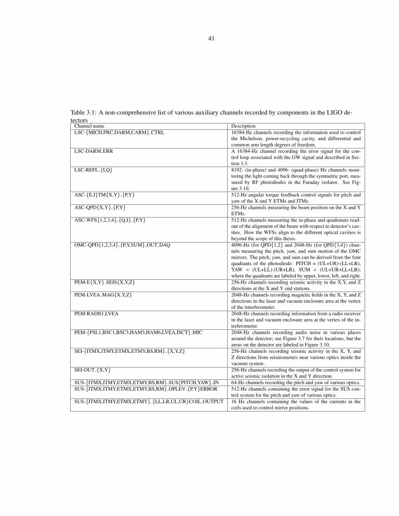
3.1 A non-comprehensive list of various auxiliary channels recorded by components in the LIGO

detectors 41

4.1 The list of channels a priori deemed unsafe due to their physical coupling to the GW channel.

Here LSC is the length-sensing and control subsystem, DARM is the differential arm motion,

OMC is the output mode cleaner, and DAQ is a data acquisition system. 67

xxxvi

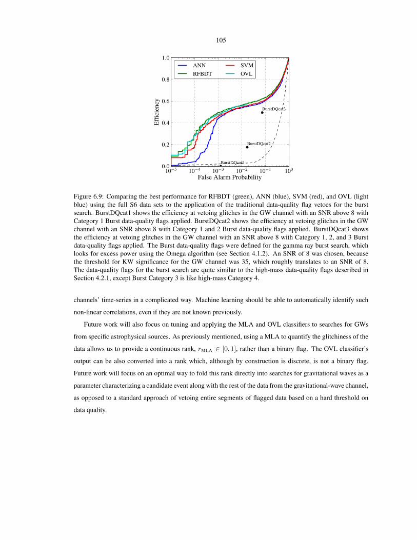
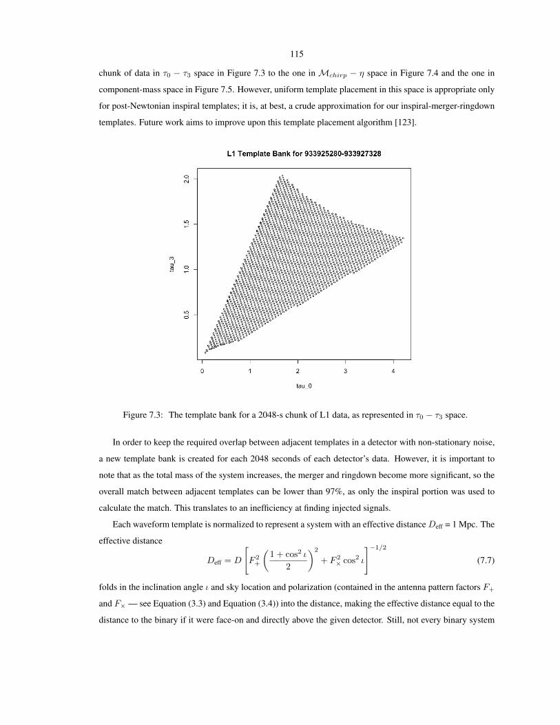
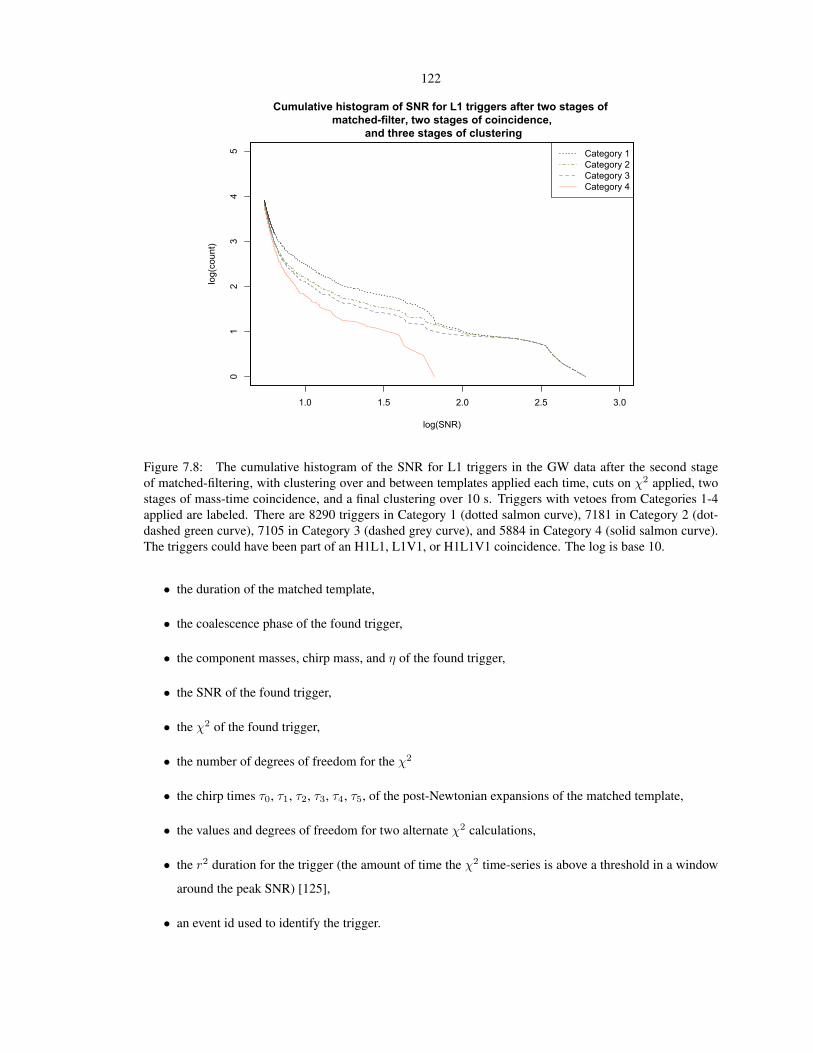
7.1 The analysis periods for S6-VSR2/3, the data from which were taken by the LIGO and Virgo

detectors from 7 July 2009 to 20 October 2010. The first three entries are from Virgo’s sec-

ond science run (VSR2) and the last two entries are from Virgo’s third science run (VSR3).

109

7.2 The total amount of coincident time (when two or more detectors were taking data) for S6-

VSR2/3, the data from which were taken by the LIGO and Virgo detectors from 7 July 2009

to 20 October 2010. The first three entries are from Virgo’s second science run (VSR2) and

the last two entries are from Virgo’s third science run (VSR3). Each detector combination

is known as an observation time, and a single observation time from an analysis period is

known as an analysis time. Note a couple cases of the analysis time going up from Cate-

gory 3 to Category 4; this is due to H1L1V1 time being turned into double time after the

application of vetoes removed a significant amount of Category 4 time for one of the detectors.

110

8.1 The false alarm rate of the loudest foreground (zerolag) event (FAR, in events per year) and the

expected false alarm rate of the loudest foreground (zerolag) event ( ˘FAR, in events per year),

for each analysis time in S6-VSR2/3. The expected loudest foreground FAR, ˘FAR, is simply

the inverse of the length of the analysis period, expressed in years. 143

8.2 The search’s sensitive distances and coalescence rate upper limits, quoted over 9M�-wide

component-mass bins labelled by their central values. We also quote the chirp massM at the

center of each bin. The sensitive distance in Mpc (averaged over the observation time and over

source sky location and orientation) is given for EOBNR waveforms in S5 data rescaled for

consistency with NR results [23], and for EOBNRv2, IMRPhenomB non-spinning (“PhenomB

nonspin”) and IMRPhenomB spinning (“PhenomB spin”) waveforms in the S6-VSR2/3 data.

The last two columns report 90%-confidence rate upper limits in units of 10−7 Mpc−3yr−1,

for bins with component mass ratios 1 ≤ m1/m2 ≤ 4, for S5 data (revised relative to [23])

and the cumulative upper limits over S5 and S6-VSR2/3 data, as presented in this work. . . . 150

xxxvii

8.3 Search sensitive distances, quoted over 9M�-wide component mass bins labelled by their cen-

tral values. The sensitive distance in Mpc (averaged over the observation time and over source

sky location and orientation) is given for EOBNR waveforms, non-spinning IMRPhenomB

waveforms, and spinning IMRPhenomB waveforms separately. Both LMVSC and ρhigh were

used as the ranking statistics for a FAR; the FAR of the expected loudest event ( ˘FAR) was

used to calculate the sensitivity. Compare to the sensitive distances listed in Table 8.2, which

were calculated using the loudest event statistic. In this table, all the sensitive distances were

calculated using a threshold at the expected loudest event, rather than at the loudest foreground

event. The rightmost column calculates the expected sensitive distance based on the steps in

Section 2.2.2, using a single-detector SNR threshold of 8 for detection and the mode average

of the L1 spectrum during S6. As L1 was usually the second most sensitive detector, this

makes it a good estimate for the sensitivity of the search. The expected sensitive distance uses

a purely Gaussian noise profile and does not take into account any complexities of our pipeline

(template bank, loudest event statistic, various vetoes and thresholds). . . . . . . . . . . . . . 172

1

Chapter 1

The search for gravitational waves fromthe coalescence of black hole binarysystems

Gravitational waves (GWs) are produced by anything with an accelerating mass quadrupole moment.

Two compact objects, such as black holes or neutron stars, that are locked in orbit together are an example of

such a system that would produce GWs in the frequency band accessible by current and near-future ground-

based detectors like LIGO and Virgo. As they orbit one another, they produce GWs, which carry energy and

angular momentum away from the system, thus causing them to spiral in towards one another and eventually

merge; this process is called compact binary coalescence (CBC). As these gravitational waves propagate

outward from the system, they stretch and squeeze spacetime in the plane perpendicular to the direction

of propagation. LIGO and Virgo detectors use (very sophisticated) Michelson interferometers to detect the

differential change in the length of two perpendicular arms.

In the ideal setting, where noise is Gaussian and stationary, the optimal detection statistic for detect-

ing GW signals in LIGO-Virgo data are the signal-to-noise-ratio from a matched-filter analysis, which is

described in Section 7.3.3. Matched-filter analysis requires that we have a bank of waveform examples (tem-

plates), which model the astrophysical signals we expect to be arriving at the detector. CBCs are unique

among the potential sources of GWs in that the inspiral portion of their gravitational waveforms have been

computed using both analytic and numerical methods. When the two objects in the binary are both black

holes, the waveforms can be extended to the merger of the two black holes and the final black hole’s ring-

down; in this case the entire signal is known as the IMR waveform. The template that gives the largest

matched-filter signal-to-noise ratio (SNR) also gives the component masses of the binary and their spin val-

ues, if any.

Unfortunately, interferometric gravitational wave detector noise is far from Gaussian or stationary. There

are a lot of instrumental artifacts and environmental disturbances that also cause a large matched-filter SNR;

these are known as glitches (see Section 4.1 for a thorough discussion of glitches). Higher mass systems

2

produce shorter waveforms in the detection band, and shorter templates are more prone to registering high

SNRs from glitches, preventing the detection of higher mass systems (and even complicating the detection of

lower-SNR signals from lower mass systems). This thesis focuses on reducing the effect of such glitches and

other artifacts of the data on the ability of the LIGO detectors to detect GWs from high-mass CBCs optimally.

1.1 The motivation for the search for gravitational waves from black

hole binary systems

Detecting the merger of two black holes, which can only be observed via the gravitational radiation

emitted, will give us information about the physics of black holes. As black holes cannot be directly detected

via observations in the electromagnetic spectrum, this is the only way to “see” them. Detecting their merger

will confirm that these objects exist and are the objects described by General Relativity (GR), or provide

direct evidence for physics beyond GR that may be required to explain the properties of such objects.

We can also verify the physics of GWs — that the emitted waves are what we expect based on the theory

of GR, whose predictions are summarized in Section 2.2.1. The most interesting part of the detection will

be the merger, when curved space smashes into curved space; this will give us insight into the strong-field,

highly dynamical, and non-linear regime of GR, which has never been observed. Another test of GR is that

of the no-hair theorem, which states that all stationary black hole solutions in GR can be described by only

three parameters: the black hole’s mass, electric charge, and angular momentum. By observing the ringdown

of the final black hole after a merger, we can check that each quasi-normal mode of the ringdown is described

by the same three parameters of BH perturbation theory [24] and confirm the no-hair theorem.

The merger of neutron star and black hole (NS+BH) and BH and solar mass BH systems is “under our

lamppost” — the frequency content of their expected GWs during and near merger is in the sensitive band

of the LIGO and Virgo detectors. Also, the amplitude of GWs emitted from a system scales with the sys-

tem’s mass; systems with tens of solar masses can be detected with advanced detectors across cosmological

distances. Therefore, although we know, due to their pulsating radio signals, that there are NS+NS systems

within advanced detectors’ astrophysical reach, the first detection of GWs from the Advanced LIGO-Virgo

detectors could come from a BH+BH merger.

Detecting the merger of NS+BH and BH+BH systems (together referred to as black hole binaries (BHBs))

will give us unique information about the nature and population of astrophysical black holes in the universe

(how big they can be, how fast they can spin). Multiple detections will in turn give us information about the

possible formation processes that lead to such systems, which can last many billions of years and are not yet

fully understood. These processes are briefly discussed in Section 2.1.

3

1.2 Issues associated with the search for high-mass CBCs

The search for high-mass (25 − 100M� total) CBCs complements the search for low-mass (1 − 25M�

total) CBCs. Numerous examples of NS+NS and low-mass NS+BH systems are known in our galaxy, and

there are no known observations of BH+BH systems. This is one of the reasons that the low-mass search and

the high-mass search are not combined into a single search. A second reason is that, as a practical matter,

for low-mass systems, inspiral-only templates are sufficient, while IMR templates are required for high-mass

binary signals. Third, higher mass templates are more likely to pick up glitches and assign these spurious

events a large SNR, which can obscure signals from lower mass systems.

Figure 1.1 illustrates the effect of widening one’s search space. The point where the background curves

(blue, cyan, black, and green) intersect the x-axis is the SNR2 of the loudest background event, below which

signals are obscured. In the presence of Gaussian noise, searching over high-mass templates in addition to

low-mass ones moves the background from the blue curve to the cyan one, which results in fewer observable

low-mass signals (red), but enables the discovery of high-mass signals (magenta); see this by drawing a

vertical line from the rightmost point of the blue/cyan curve to where it intersects with the red/magenta

curves. In the presence of non-Gaussian noise, searching over low-mass templates results in the background

curve picking up a non-Gaussian tail (compare the black curve to the blue curve). Searching over high-mass

and low-mass templates in the presence of non-Gaussian noise also results in the background curve picking

up a non-Gaussian tail, but in this case, the tail is much fatter and longer (compare the green curve to the cyan

curve). This is because the high-mass templates are shorter and thus more likely to pick up non-Gaussian

glitches, since they have similar timescales.

For these reasons, we search separately for low-mass and high-mass signals. This thesis will explore

ways to reduce the extent of the non-Gaussian tail.

1.3 Mitigating the effect of glitches in the search for high-mass CBCs

This thesis focuses on mitigating the effects of glitches on the search for high-mass CBCs in LIGO-Virgo

data. We perform several steps to reduce the number of glitches we have to sift through before finding a

genuine GW. First, we carefully examine the quality of the data in each detector and do not analyze data if

the detector is not functioning satisfactorily (see Chapter 4). Second, we enforce coincidence — a trigger

must be seen by at least two detectors from the three: LIGO-Livingston, LIGO-Washington, and Virgo-Italy

(see Section 7.3.4). Third, thresholding on the result of a χ2 test, which measures how well the template

matches the data in different frequency bands, allows the rejection of a large fraction of single-detector

glitches (see Section 7.3.6). Ideally, we would also enforce coherence between the signals seen in the two

or more detectors, and others are working on this tactic. However, most of our triggers are found in double

coincidence, and a coherent step is only helpful when there are 3 or more detectors, to provide a constraint

4

50 100 150 200 250 300 350 400100

101

102

103

Cumulative histogram of SNR2 distributions

SNR2

Num

ber o

f eve

nts

with

SN

R2 > x

Figure 1.1: A cartoon plot representing the overlap of signal and background in different situations. Blue:Background triggers due to Gaussian noise, picked up by a search with low-mass templates. Cyan: Back-ground triggers due to Gaussian noise, picked up by a search with low-mass and high-mass templates. Black:Background triggers due to Gaussian and non-Gaussian noise, picked up by a search with low-mass tem-plates. Green: Background triggers due to Gaussian and non-Gaussian noise, picked up by a search withlow-mass and high-mass templates. Red: Theoretical signal distribution for low-mass astrophysical signals.Magenta: Theoretical signal distribution for low-mass and high-mass astrophysical signals, assuming thereare an equal number of each.

in the presence of the two polarizations of GWs (see Section 2.2.1). In the end, we are still left with a lot of

glitches littering our lists of loudest candidate GW events produced by our detection pipeline.

This problem is worse for the types of signals we expect to be arriving from higher-mass compact binary

systems, as the duration of their inspiral waveform is relatively shorter — closer to the timescale of glitches,

i.e., on the order of a second or less. In the LIGO-Virgo searches for these coalescing compact binary

systems (see Chapter 7 for a summary of the literature), we reweight the SNR by the χ2, as glitches tend to

have a worse/higher χ2 than real GWs would. The distributions of this reweighted SNR are a lot closer to

the Gaussian limit, especially for lower mass systems (1 − 25M� total); however, there is room for much

improvement in the search for gravitational waves from higher mass systems (25− 100M� total).

By combining SNR and χ2 in this way, we are able to create a detection statistic that better separates our

background events from our simulated signal events than the theoretical ideal, the matched-filter SNR, alone.

However, the matched-filter outputs more than just SNR and χ2; we can also easily examine the templates

found in the different detectors for closeness. For example, if there are signals at two detectors at the exact

5

same time, but the template matched in one detector is for a neutron star and a 25 solar mass black hole and

the template matched in the other detector is for two 25M� black holes, one can surmise that the two signals

are really glitches that occurred at the same time due to unlucky coincidence.

The search can surely be improved by folding the template parameters and the time difference between the

signal arrivals at the different detectors into the detection statistic. However, this proves to be quite challeng-

ing to do analytically, as humans can only really process two-dimensional correlations at once, maybe three.

Moreover, in a single dimension, the distribution of values overlaps significantly between our signal distribu-

tion and background distribution; see the red versus black distributions in the histograms in Section 8.3.1.4.

We could use numerical solutions, for example, a series of two dimensional likelihood calculations, but this is

not computationally feasible for the hundreds of thousands of coincident events produced by the LIGO-Virgo

system of detectors.

Multivariate statistical classification is the perfect tool to incorporate all the information from a matched-

filter analysis into a single detection statistic. Section 5.3 will describe the multivariate method used, and

Section 8.3.1.6 quantifies how it improves the search.

It can also be used to identify times when the detector is likely to be especially glitchy, without looking

at the GW channel itself. The efforts in this realm are discussed in Chapter 6.

6

Chapter 2

The physics and astrophysics ofgravitational waves from compactbinary coalescences with total mass of25 − 100 M�

2.1 Astrophysics of compact binaries with two black holes or one black

hole and one neutron star

The likelihood of detecting coalescing BH+BH or BH+NS systems necessarily depends on the number of

such binaries within our detection volume and the timescales at which they will merge. Since such systems

have never been directly observed (in our Galaxy or extragalactically), the rate for such detections with LIGO

is extremely uncertain. These rates are based largely on models attempting to synthesize the population of

compact binaries in Milky Way-like galaxies, via two formation scenarios: Isolated Binary Evolution (IBE)

and Dynamical-Formation Scenarios. These processes and their expected rates will be briefly discussed in

the following subsections.

The LIGO-Virgo Collaboration (LVC) has agreed on a set of astrophysical predictions of how many

events LIGO will see, summarized in Table 2.1 [21]. Please note that because many configurations of

numerical simulations of IBE do not produce black holes much more massive than 10 M� (as explained in

Section 2.1.2), the estimates for BH+BH merger are for two 10M� black holes, which is actually searched for

with the LIGO low-mass search; our high-mass search begins at a total mass of 25 M�. The estimates for an

intermediate mass ratio inspiral (IMRI) with an intermediate mass black hole (IMBH) take into consideration

many Dynamical-Formation Scenarios, but focus on a stellar mass object (NS or BH) into an IMBH between

50 and 350 M�. (Note that the literature is not consistent on the mass range defined by IMBH). There are

regions of the high-mass search that are ignored by this table (e.g. a 25M� on 25M� system). Nonetheless,

Table 2.1 is presented for as an “official” set of expectations by the LVC.

7

Black holes with masses in the ranges considered in our search for high-mass CBCs are predicted via

computer simulations, see Figure 2.1 [20]. But, as will become clear in the following sections, there is a lot

of uncertainty in the ways such systems can evolve, how many there are, and what masses they can have.

In the future, as the LVC makes (or doesn’t make) detections of CBCs, we can constrain the astrophysical

models of stellar and galactic evolution.

Figure 2.1: The mass distributions of various kinds of single BHs at 11 Myr based on simulations usingReference [1]’s standard model (A). The dotted line indicates BHs evolved from primordial single stars; thedashed line shows single BHs from disrupted binaries; and the solid line shows single BHs that are remnantsof merged binaries. The bin width is 2.0 M�and the counts are normalized to the total number of BHs [1].

2.1.1 Isolated binary evolution

In isolated binary evolution (IBE), two massive stars form from a common progenitor gas cloud and form

a binary. After some time, one star undergoes core collapse supernova and turns into a NS or a BH, but in rare

cases (of interest here), the mass loss in the supernova is low enough that the binary survives the event. Some

time later, the same thing happens to the other star, leaving a double compact object (NS+NS, NS+BH, or

BH+BH) which will eventually become a coalescing binary system [25]. During the evolution of the system,

there are many paths that can be taken that do not lead to the formation of the a CBC. For example, in a

simple model where two stars are in a circular orbit and one goes supernova, but does not happen to receive

a kick, the stars only remain bound if the mass loss from the supernova is less than half of the original total

mass [26]. Moreover, even if a BHB does form, if there is no common envelope phase during the supernova,

the resulting compact objects will likely be too far apart to merge within the age of the universe [27].

The common envelope phase(s) are important in that they decrease the orbital separation of the binary,

but they can also inhibit the production of a number of BHB systems. The common envelope phase can

result in the two stars merging via dynamical friction rather than via gravitational wave emission. This

process especially inhibits the production of close high-mass BH+BH binaries when the donor star is evolving

8

Table 2.1: Detection rates for compact binary coalescence sources, from Reference [20], an extensiveliterature search. Please refer to Reference [20] for details on each estimate. The Initial LIGO rates arebased on a horizon distance of 33 Mpc for an optimally oriented 1.4+1.4 M� NS+NS system, 70 Mpc for anoptimally oriented 1.4+10 M� NS+BH system, and 161 Mpc for an optimally oriented 10+10 M� BH+BHsystem. These horizon distances are 445, 927, and 2187 Mpc, respectively, for Advanced LIGO [20]. Theintermediate mass ratio inspiral (IMRI) is taken to be a solar mass object spiraling into an intermediatemass black hole (IMBH) having a mass between 50 and 350 M�The rates for these systems are take fromReference [21]’s considerations on 3-body hardening in globular clusters. The rates for IMBH+IMBHringdown signals are taken from Reference [22]’s considerations of N-body interactions in young star clusters.

IFO Source Nlow Nre Nhigh Nmax

yr−1 yr−1 yr−1 yr−1

NS-NS 2× 10−4 0.02 0.2 0.6NS-BH 7× 10−5 0.004 0.1

Initial BH-BH 2× 10−4 0.007 0.5IMRI into IMBH < 0.001 0.01

IMBH-IMBH 10−4 10−3

NS-NS 0.4 40 400 1000NS-BH 0.2 10 300

Advanced BH-BH 0.4 20 1000IMRI into IMBH 10 300

IMBH-IMBH 0.1 1

through the Hertzsprung Gap (increasing in radius). If there were no common envelope evolution during

the radius increase, there would be hundreds of times more possible detections [28]. In Figure 2.2, the

difference between Model B (bottom 2 panels), in which the progenitor stars merge if the common envelope

phase is initiated by a Herzsprung gap star, and Model A (top two panels), in which progenitor stars are

allowed to remain distinct and can continue evolving into a double compact object, is shown; the result is

that Model B has many fewer resultant double compact objects, which also have a much lower chirp mass

(see Equation (2.14)) [2]. If the stars can evolve through the Hertzsprung Gap before the common envelope

phase, their centers can be further apart. This is important, because if the stars start off too close together,

they can end up merging via tidal effects before turning into compact objects [27].

If the progenitor stars are massive enough, a supernova is not needed to produce a compact object. At

around and above 100 M�, the star’s core can be so massive that it collapses without a supernova explosion

[27]. This allows the resultant BH to retain most of the mass of its parent star.

The spins of the compact-objects-produced IBE scenarios tend to be aligned, since their massive pro-

genitor stars probably had their spins aligned with the orbital axis (since they were born from the same gas

cloud). Even if fragmentation of the gas cloud occurred [29], strong torques along the orbital axis encourage

spin-orbital alignment [27]. If one of the black holes received a kick from a supernova, the spins could be

misaligned, but this would be rare, since kicks tend to disrupt the binary. Detection of GWs from these sys-

tems will allow us to determine the masses and spins of the system producing the GWs, and give us insight

into the way the BHB was formed. For example, since core-collapse (with no supernova) produces BHs with

no mass (and angular momentum) loss, these BHs will be spinning very rapidly.

9

Of course, the predicted masses and spins of the BHB systems are very sensitive to the computer simula-

tions’ inputs and code itself. The methods for these simulations are introduced in the following section.

2.1.2 Population synthesis

The stellar and binary populations resulting from IBE are often estimated via population synthesis, the

umbrella term for a family of computer simulation methods; the results of which are useful for the LVC

because they estimate how many pairs of zero-age main sequence stars turn into compact binaries.

For IBE, a single simulation creates a model for primordial stars, sets up rules for the stars’ evolutions,

and then sets the model to evolving. Of course, there are a lot of assumptions/choices one must make for

the initial conditions that are entered into the simulation. In practice, a distribution of reasonable ranges for

the flexible parameters is chosen and a Monte Carlo is done over the parameter space; this results in many

possible futures for a set of primordial stars, but only those that are consistent with astrophysical observations

are considered in the end. Because of the dependence on sanity checking end results against astrophysical

observations, which historically have been dominated by galactic NS+NS systems, most past results have only

been valid for Milky Way-like galaxies (i.e. spiral galaxies). The results quoted in [21] are from simulations

done only for Milky Way-like galaxies. Unfortunately, spiral galaxies just don’t produce that many BH+BH

systems because the stars forming the progenitors are not sufficiently massive, but the initial mass function for

elliptical galaxies is much shallower, allowing for a greater proportion of high mass zero age main sequence

stars [30].

Another key peculiarity about the simulations used to predict BH+BH mergers in [21] is that the metal-

licity of stars is usually assumed to be solar metallicity [31]. Metallicity refers to the atomic content of stars.

There are many ways of measuring metallicity; one way is Z, the fraction of the star’s chemical composition

that is not hydrogen and helium. Our sun, a Population I star, has Z = 0.02 [32]. Though this is a relatively

high metallicity itself, high-metallicity stars are generally categorized by having a metallicity greater than

that of our sun. High-metallicity stars are second generation stars (Population I) — they are made of the

recycled material from the supernova of their parent star [33]. High-metallicity stars tend to be lighter than

low-metallicity stars because of stellar wind effects — photons ejected by the star hit the electron cloud of

the metal atoms in the outer layer of the star and push them out [34]. In contrast, low-metallicity stars’ outer

layers are more transparent to photons and therefore are not subject to significant mass loss before they have

the opportunity to undergo core collapse and potentially turn into a black hole. This effect is twofold relevant

to the search for high-mass CBCs: first, the mass of the final black holes can be larger, thus increasing the

distance to which we are sensitive to these systems; second, the higher masses make the likelihood of a large

natal kick much lower, so the black hole is more likely to stay in the binary. The effect of metallicity on

the number and mass distributions of resultant double compact objects in population synthesis is shown in

Figure 2.2 [2]. Note that only in the second panel (low rate of common envelope merger and low metallicity)

are there a significant number of high mass BH+BH systems. In reality, stars will probably have a range of

10

metallicities between these values [35].6

Fig. 1.— Chirp mass distribution for double compact objects. Top two panels: Model A. Note the strong e!ect ofmetallicity on chirp mass of binaries with black holes. Low metallicity (2nd panel down) reduces the wind mass loss fromthe BH progenitors, allowing more massive BHs to form. The maximum chirp mass is ! 8 M! for solar composition,while it can reach ! 30 M! for 10% solar for BH-BH mergers. Bottom two panels: Model B. Note that BH binariesappear (in significant numbers) only in the low metallicity case (bottom panel). The typical chirp mass in model B issignificantly lower than in model A. This is the result of progenitor elimination through common envelope mergers inmodel B. In particular, high mass stars (that can give birth to the highest mass BHs) reach large radii and are proneto enter a common envelope phase while crossing the Hertzsprung gap, thereby aborting further evolution even at lowmetallicity.

Figure 2.2: Histograms of number versus chirp mass for 4 different Population Synthesis scenarios [2]. Thetop two panels are for simulations of category A, in which progenitor stars are allowed to remain distinct andcan continue evolving into a double compact object even if the donor star is evolving through the Hertzsprunggap during the common envelope phase; the bottom two are for category B, in which the progenitor starsmerge if the common envelope phase is initiated by a Herzsprung gap star. Note that for both A and B,both the number of, and the maximum chirp mass (which, as we will see in Section 2.2.1, is the relevantcombination of component masses used for describing CBCs) increase for the systems with 10 percent solarmetallicity (second and fourth panels) [2].

2.1.3 Dynamical formation scenarios

Interactions between black holes in dense cluster environments can also lead to close BH+BH sys-

tems [36]. There are three main dynamical formation scenarios that can lead to a high-mass black hole

binary system: 1) N-body interactions in globular clusters, 2) 2-body scattering in Galactic nuclei, 3) 3-body

interactions involving black holes in galactic nuclei [21]. The theory behind such interactions and the obser-

vational evidence constraining them is much weaker than for IBE, but they can produce more black holes in

the mass range relevant to this thesis, and the detection of such systems can inform the astrophysics [37].

11

2.1.3.1 Globular clusters

Globular clusters are very tightly bound by gravity, which gives them their spherical shapes and relatively

high stellar densities toward their centers (mass segregation). In the dense environment, high-mass stars

quickly evolve via supernova into black holes. These massive black holes fall further toward the center,

where they meet with other black holes, which will quickly break up any remaining star-BH binaries. During

this interaction, the BHs acquire kinetic energy and can be ejected from the cluster as either single BHs or

binaries. This entire process is known as segregation, decoupling, and evaporation [37]. These binaries can

merge much more quickly than those produced by IBE, since the interactions with the other nearby objects

cause the binary to “harden” (i.e. for the orbital separation to decrease) [27].

Since BH+BH binaries produced from dynamical cluster evaporation do not rely on supernova kicks,

common envelopes, or mass transfer to bring them close enough to merge in a Hubble time, their masses can

be higher, see Figure 2.3 [3]. Their spins and orbital angular momenta are not aligned in any way because

interactions tilt the orbital plane [27].

Future gravitational wave observations will provide very useful astrophysical information to this field

by more tightly constraining gcl (the fraction of stars formed in clusters) and gevap (the fraction of cluster-

forming mass with birth conditions that could lead to segregation, decoupling, and evaporation). Weak obser-

vational constraints combined with numerical simulations yield gclgevap = 5 × 10−2, leading to a plausible

but optimistic rate listed as Nhigh of IMBH+IMBH mergers in Table 2.1.10 O’Leary et al.

FIG. 4.— Chirp mass of mergers versus time. This is a comparison of the two models v2e5k11 and v22e6e5k9, in panels (a) and (b) respectively. Plotted is thechirp mass versus time of all mergers of 46 random runs of model v2e5k11 and all 46 runs of v22e6e5k9. Model v2e5k11 is one of the least efficient clusters inproducing large BHs and BH–BH binary mergers in general. Therefore, the distribution is most nearly that expected from the initial mass distribution of BSR04.Because of how quickly v2e5k11 evolves (teq ! 200Myr) almost all mergers in later times occur outside the cluster. In comparison, v22e6e5k9 is a massivecluster that does not reach equipartition before a Hubble time. There is still a significant fraction of BHs in the cluster at the end of the simulation, which allowsfor more growth, and also more massive BH mergers.

FIG. 5.— Merger rate vs. time. The solid curve is the average mergerrate of model v2e55k9 as a function of time. The dotted line is a power–law " time!1. After # 108 yr, the merger rate is inversely proportional to theage of the cluster. The evolution of the merger rates can be split into twophases. The first when the cluster is undergoing many binary interactions,and the second, when the binary fraction is depleted and nearly zero. Thesetwo phases of merger rates appear consistently in all cluster models.

with other measurements: H0 = 71km s!1 Mpc!1, !m = 0.27,!! = 5!10!5, and !! = .73.In our calculations, we assume that the globular cluster

model was formed uniformly through the universe at a givencosmological time corresponding to redshift zform. We thenrecord each detectable merger into one of 100 bins each withtime width !t = t0/100, where t0 is the current age of the uni-verse, based on when the merger occurred. If di is the number

FIG. 6.— Energy distribution of ejected BH binaries. Plotted is the proba-bility distribution of the energy of all BH–BH binaries ejected before equipar-tition in 117 runs of model v2e55k9. The energy is plotted in units of themean kinetic energy kT , where 3/2kT is the mean stellar kinetic energy ofthe MS stars in the core of a cluster of this type. We find that all other modelshave a distribution very similar to the one shown above.

of detections in bin i, we sum over the rate of each bin givingthe final rate:

Rzform =100!

i=1

di!t4"3

#0(D3i !D3i!1)(1+ zi)!1, (13)

where #0 is the current density of a given cluster model and ziis the redshift to bin i. With te = t0 ! i!t, the proper distance to

Figure 2.3: A comparison of two numerical simulations of BH pair formation in globular clusters. The leftpanel (a) shows the least efficient (out of 46 simulations) cluster, in terms of producing large BHs and BH+BHbinaries. The right panel (b) does not reach equipartition (when the rate of BH interactions with other starsin the cluster is less than or equal to the rate of BHs with other BHs) before a Hubble time; therefore, thereare many more BHs in the cluster — allowing the formation of many more binaries. The x-axis is time sincethe beginning of the simulation (11 Myr after the Big Bang) [3].

12

2.1.3.2 Galactic nuclei

A galactic nucleus with a supermassive black hole and many stellar-mass black holes will have steep

density cusps, which allow the formation of tight BH+BH binaries directly via 2-body scattering. In this

scenario, an encounter between two BHs that would initially be hyperbolic, can lead to capture via energy

loss due to gravitational radiation (Bremsstrahlung) during the point when the two BHs are closest together.

These binaries tend to be eccentric and coalesce on a timescale of hours; in fact, they are still eccentric when

they enter the LIGO band [38].

In the nuclear clusters of small galaxies without a supermassive black hole, 3-body interactions cause

wide BH+BH binaries to tighten more quickly than they would in an isolated scenario, allowing the radiation

reaction to lead them into inspiral. Similar to what has been observed in triple star systems, the two most

massive objects form a binary; the third object orbits the binary and is close and massive enough to interact

with it and affect the eccentricity of the binary. The eccentricity oscillates (the oscillations are referred

to as Kozai cycles), which causes the binary’s orbit to harden more quickly than if it were isolated — an

eccentric binary will tend to circularize as the orbital separation decreases, which in turn decreases the rate

of hardening [27].

There are no established predictions for the number of BH+BH or BH+NS systems (with total mass

between 25 and 100 M�) from 2-body scattering or N-body interactions in globular clusters. If the BHs are

approximately of solar mass, Reference [39] predicts a “few × 10−2” mergers per nuclear cluster per Myr.

Reference [27] predicts that all dynamical formation scenarios could produce 10 BH+BH mergers (with total

mass around and above 100 M�) per cubic Mpc per Myr. Such mergers would not have spins aligned with

their orbits, because orbital tilting is produced during the cycles [27].

2.1.4 Observational evidence from low-metallicity galaxies

There have recently been observed two extragalactic X-ray binaries in low-metallicity environments:

IC10 X-1 and NGC300 X-1. Each system is thought to consist of a BH with mass ∼ 20 - 30 M� accreting

from a massive Wolf-Rayet (WR) star companion with mass & 20 M�. Models predict that these systems

will evolve into BH+BH binaries with chirp masses of about 15 M� within 3 Gyr. Extrapolating from the

fact that there are 2 of these systems within 2 Mpc, we estimate a detection rate of R = 3.4+8.3−2.9 detections

per year at the 99 percent confidence level, for initial LIGO [40]. That no such signals were found in initial

LIGO/Virgo data allows us to rule out the upper end of this predicted rate.

Measuring the rates via future GW observations will allow us to tune the knobs of the population synthesis

models, have a better understanding of low versus high metallicity environments, and gain a deeper analytical

understanding of the different stages of stellar evolution [40].

13

2.2 The physics of gravitational waves from compact binary coales-

cences

2.2.1 The mathematical formulation of gravitational waves

Gravitational waves are a theoretical consequence of Einstein’s theory of General Relativity. The funda-

mental equations of this theory, relating the curvature of spacetime to matter/energy are

Gαβ =8πG

c4Tαβ , (2.1)

where Gαβ , a function of the spacetime metric gab and its derivatives, is the Einstein tensor describing the

curvature of spacetime and Tαβ is the stress-energy tensor. G and c are the gravitational constant and the

speed of light, respectively. α and β run over time and three spatial coordinates. The theory and formalism

used in this section follow those of the book “Gravitational-Wave Physics and Astronomy: An Introduction

to Theory, Experiment and Data Analysis” by Jolien D.E. Creighton and Warren G. Anderson.

In linearized gravity, the general spacetime metric can be expressed as the flat Minkowski metric ηαβ

plus some perturbation hαβ :

gαβ = ηαβ + hαβ . (2.2)

It is useful to use the trace-reversed metric perturbation instead, which is given by

hαβ = hαβ −1

2ηαβ . (2.3)

Then, in the Lorenz gauge (where the divergence of the trace-reversed metric is zero), the linearized Einstein

equations become

�hαβ =8πG

c4Tαβ , (2.4)

where� is the d’Alembert operator [41], which is the Laplacian generalized to 4-dimensional flat (Minkowski)

spacetime.

In a vacuum, this becomes

�hαβ = 0, (2.5)

which we recognize as a wave equation. We can choose a plane-wave solution traveling in the z direction. By

combining Equation (2.5) and Equation (2.3), we see that the non-vanishing parts of the trace-reversed metric

are hxx, hxy , hyx, and hyy , which are all functions of (t − z/c). This corresponds to a metric perturbation

traveling at the speed of light along the z axis [41].

Independent of gauge, there are two independent functions of (t − z/c) that come out of these equa-

tions. These will be called h+ and h× and are the two polarizations of these transverse waves (the so-called

14

gravitational waves referred to in this thesis) [41].

The energy carried by these waves is

TGWtt =c4

16πG〈h+

2+ h×

2〉 ∝ ω2, (2.6)

where TGWtt is the time-time component of the stress-energy tensor associated with the GW and ω is the

angular frequency of the wave [41].

In the transverse traceless gauge (denoted TT ), the form of the metric perturbation both far (characteristic

size of the source� GW wavelength� distance to the source r) from and near (GW wavelength� distance

to the source r� characteristic size of the source) to the source is, under the quadrupole approximation,

hTTij '2G

c4rITT (t− r/c), (2.7)

where r is the distance to the source and ITTij is the quadrupole tensor of the source in the transverse traceless

gauge, given by

ITTij =

∫ (||−→x ||2δij − xixj

)ρ(−→x )d3−→x . (2.8)

Note that in this gauge, h×=hxy and h+=hxx. In the quadrupole approximation, higher moments of inertia

are ignored because the quadrupole moment dominates [41].

For an orbiting compact binary system, under the quadrupole approximation, the form of the two polar-

izations of the metric perturbation looks like this far from the source:

h+(t(β)) = −2Gµ

c2r(1 + cos2 ι)β2 cos 2φ(β), (2.9)

h×(t(β)) = −4Gµ

c2rcos ιβ2 sin 2φ(β), (2.10)

where µ is the reduced mass µ = m1m2/(m1 + m2), ι is the inclination angle from the observer to the

source, φ(β) tracks the orbital phase, and β is the characteristic velocity of the center of mass system divided

by the speed of light (v/c), which can be used as a proxy for the orbital frequency, ω, or orbital separation,

a, thanks to Kepler’s law,

β =3√GMω

c=

√GM

ac2. (2.11)

From Equation (2.5) and Equation (2.11), one can see that as the orbit gets smaller, the frequency of the

gravitational wave increases, as does its amplitude; this is known as a chirp signal [41].

15

Using the quasi-Newtonian formalism (note that Newton’s laws say the binary orbit is stable, but in the

literature this is nonetheless sometimes referred to as Newtonian), which is applicable when the orbit is not

yet relativistic, the GW frequency

f = 2forb = ω/π (2.12)

evolves likedf

dt=

96

5π8/3GM

c3

5/3

f11/3, (2.13)

where

M = (m1m2)3/5(m1 +m2)−1/5 (2.14)

is known as the chirp mass. This quantity is important because the lowest-order (in β) term in the CBC

waveform depends only on the chirp mass, not the mass ratio. The chirp mass can also be expressed as

M = Mtotalη3/5, (2.15)

where Mtotal = m1 +m2, and

η =m1m2

M2total

. (2.16)

If we integrate Equation (2.13) from an arbitrary time to the time of coalescence, tc, we get

h+(t) = −2GMc2r

(1 + cos2 ι)

2

(c3(tc − t)

5GM

)−1/4

cos

[2φc − 2

(c3(tc − t)

5GM

)5/8]

(2.17)

h×(t) = −2GMc2r

cos ι

(c3(tc − t)

5GM

)−1/4

sin

[2φc − 2

(c3(tc − t)

5GM

)5/8]

(2.18)

as the representations of the inspiral portion of the waveform in the time domain; note that h+ and h× are

unitless and represent a strain. The effect of the different polarizations can be illustrated by imagining a ring

of particles in the plane perpendicular to the direction of propagation. The h+ polarization will alternately

stretch the circle in the x-direction (while squeezing it in the y-direction), then stretch the circle in the y-

direction (while squeezing it in the x-direction). The h× polarization has the same effect on the circle, but

rotated by π/2; see Figure 2.4. The polarization content of GWs reaching an observer depends solely on the

inclination angle ι. If ι = 0, the plane of the binary orbit is face-on to the observer, and the GW has equal

amounts of h+ and h× (circular polarization). If ι = π/2, the plane of the binary orbit is edge-on to the

observer, and the GW is only h+ (linear polarization).

In the frequency domain, which is used for LIGO/Virgo data analysis, the leading post-Newtonian (PN)

order term of the chirp waveform looks like

h(f) =

∫ ∞

−∞e−2πift(h+ + ih×)dt = Af−7/6eiψ(f)+iπ/4, (2.19)

16

Figure 2.4: The effect of gravitational waves on a circle of particles in a plane perpendicular to the direction ofpropagation. The left panel shows a purely plus-polarized GW. During a full period of the GW, the particlesgo from circle to horizontal ellipse to circle to vertical ellipse back to circle. The right panel shows a purelycross-polarized GW.

where Ψ(f) describes the phase evolution and

A =C

rπ2/3

√5

24M5/6, (2.20)

where C is a function of the antenna pattern of the detector (see Figure 3.11) and inclination angle ι. r is

the distance to the source and M is the chirp mass. Note that Equation (2.19) uses the stationary phase

approximation (that the frequency of the wave changes slowly during the inspiral) [41]; the full waveform

can be found in [42].

PN theory uses Taylor expansions in β to calculate waveforms that are accurate up to the final stages of

the inspiral and, notably, can be used in the generic case where both compact objects are spinning in any

direction. Inspiral-only waveforms have been calculated up to corrections β7 (this is known in the literature

as the parametrized post-Newtonian (PPN) order 3.5). However, near merger, the PPN expansion breaks

down and other methods are required because as the two bodies get closer together, higher order radiative

effects and non-linear dynamics significantly alter the waveform. NR is needed to calculate the waveform

for these last few inspiral cycles and merger. See Reference [43] for an overview of NR methods for NS+BH

systems. There have been many NR simulations done for non-spinning (see Figure 2.5) and aligned spin

systems, but current progress is being made on a full catalog of non-aligned spin waveforms, which look

significantly different due to precession effects (see Figure 2.6). After the merger, in the case of 2 black

holes, the ringdown is described analytically as a superposition of quasinormal modes [44].

The following two subsections describe the two methods used to compute the full IMR waveforms used

in this thesis; a more in-depth comparison of PN templates can be found in [45] and full IMR waveforms

in [44] and [46]. The waveforms used in this thesis are both for nonspinning and aligned spin systems, which

is reasonable but not complete — as seen in Section 2.1, IBE tends to produce binaries with aligned spin,

but there is no reason to suspect this for dynamical formation scenarios. The waveforms for non-aligned spin

17

systems look significantly different because the spin-orbit coupling of non-aligned spins causes the plane of

the orbit to precess, which causes amplitude and phase fluctuations in the waveform seen in the detector [47];

see Section 3.2 for a discussion of a detector’s response to a passing GW.

The waveform for a specific system can look significantly different depending on the waveform family

used to parametrize it. Table 2.2 and Table 2.3 show how even the number of cycles differ for the different

families.

Figure 2.5: A screenshot from a Caltech-Cornell NR simulation of two equal-mass nonspinning black holes.Visit for the full movie and more animated simulations.

2.2.1.1 Effective-one-body + numerical relativity (EOBNR) waveforms

The EOBNR waveforms combine the effective-one-body (EOBNR) formalism with NR results. effective-

one-body (EOB) methods map the dynamics onto a test particle in an external effective metric. Though the

EOB equations can be expressed analytically, what is done in practice is a non-perturbative resummation

of the PN expansion of the equations of motion [48]. For a single system, EOB waveforms are calculated

for each leading l,m mode (using spherical harmonic notation), but still have a few tunable parameters.

Each waveform is calculated separately in two parts: the inspiral-plunge and the merger-ringdown. For

the systems whose waveforms have been calculated with NR, Buonanno et al. calibrate the inspiral-plunge

EOB waveforms against the NR waveforms and set the tunable parameters to achieve the greatest amplitude

and phase consistency between the two [49]. The inspiral-plunge waveform is then stitched to the merger-

ringdown waveform, which is a sum of 8 quasinormal modes. The tuned EOBNR waveforms used in the

18

Figure 2.6: A screenshot, at merger, from a NR simulation of two black holes with a mass ratio of 6:1and non-aligned spins of .91 and .3, respectively. Note the amplitude and phase modulation, which is dueto the precession of the orbital plane resulting from the spin-orbit coupling of the non-aligned spins. Visithttp://www.black-holes.org/explore2.html for the full movie and more animated simulations.

search for high-mass CBCs have been tuned using NR for mass ratios m1/m2 = 1, 2, 3, 4 ,6 and total masses

M = 20− 200M� [49].

There are two different versions of EOBNR waveforms used in this thesis. EOBNRv1 is used, for his-

torical reasons, to create the template banks as discussed in Section 7.3.2. EOBNRv2 is used to create the

simulated signals we use to test the sensitivity of our pipeline and create upper limits. Though the EOBNR

approach works for waveforms from systems where the compact objects are spinning, the code was not re-

viewed in time for it to be included in the search described in this thesis. Figure 2.7 and Figure 2.8 show

the EOBNRv2 waveforms for the equal-mass case, as compared to the waveforms discussed in the following

section. Although EOBNRv2 waveforms were only tested for mass ratios up to 6, they should be valid in the

limit of large mass ratios, as they are created on the model of a test particle orbiting an effective potential;

Figure 2.9 and Figure 2.10 show these EOBNRv2 waveforms for the asymmetric mass ratios on the template

bank for the highmass search (25 - 100 M�).

The EOBNR waveforms are created in the time domain and are fast-Fourier transformed (FFTed) before

they are used in the analysis. The FFT waveform multiplied by the square root of the frequency can be laid

atop the strain amplitude sensitivity of the detectors, allowing us to easily visualize our ability to detect a

particular signal. The strain amplitude sensitivity of the detectors is a result of design choices and known and

unknown noise sources, which will be described in Section 3.4.

19

Figure 2.7: Time-domain waveforms for a 12.5 M�+ 12.5 M�system.

20

Figure 2.8: Time-domain waveforms for a 45 M�+ 45 M�system.

21

Figure 2.9: An EOBNRv2 time-domain waveform for a 1 M�+ 24 M�system. Note that the merger andringdown are present even though not visible due to the scale of the plot. The IMRPhenomB waveform is notplotted, as it is not valid for this mass ratio.

22

Figure 2.10: An EOBNRv2 time-domain waveform for a 1 M�+ 99 M�system. The IMRPhenomB wave-form is not plotted, as it is not valid for this mass ratio.

23

Figure 2.11: Waveforms for a 12.5 M�+ 12.5 M� system in the frequency domain, compared to the modeof H1’s noise amplitude spectral density during S6 [4]. The EOBNR waveform was originally in the timedomain, and was fast Fourier transformed into the frequency domain, resulting in non-physical wiggles. Thegreen dashed curve indicates the frequency journey of an inspiral-only waveform, whose amplitude has beenset by the IMRPhenomB waveform. Merger is short and has an undefined duration. The Fourier transformof a ringdown is the imaginary part of a Lorentzian, and can be seen in this plot beginning when the blue orred curve deviates (has a less steep slope) from the green dashed curve and continuing through the steepernegative slope towards the right of the plot, remembering that the wiggles on the blue curve are non-physical.

24

Figure 2.12: Waveforms for a 50M�+ 50M� system in the frequency domain, compared to the mode of H1’snoise amplitude spectral density during S6 [4]. The EOBNR waveform was originally in the time domain,and was fast Fourier transformed into the frequency domain, resulting in non-physical wiggles throughout thewaveform, since the waveform has a finite duration. The green dashed curve indicates the frequency journeyof an inspiral-only waveform, whose amplitude has been set by the IMRPhenomB waveform. Merger is shortand has an undefined duration. The Fourier transform of a ringdown is the imaginary part of a Lorentzian, andcan be seen in this plot beginning when the blue or red curve deviates (has a less steep slope) from the greendashed curve and continuing through the steeper negative slope towards the right of the plot, rememberingthat the wiggles on the blue curve are non-physical.

25

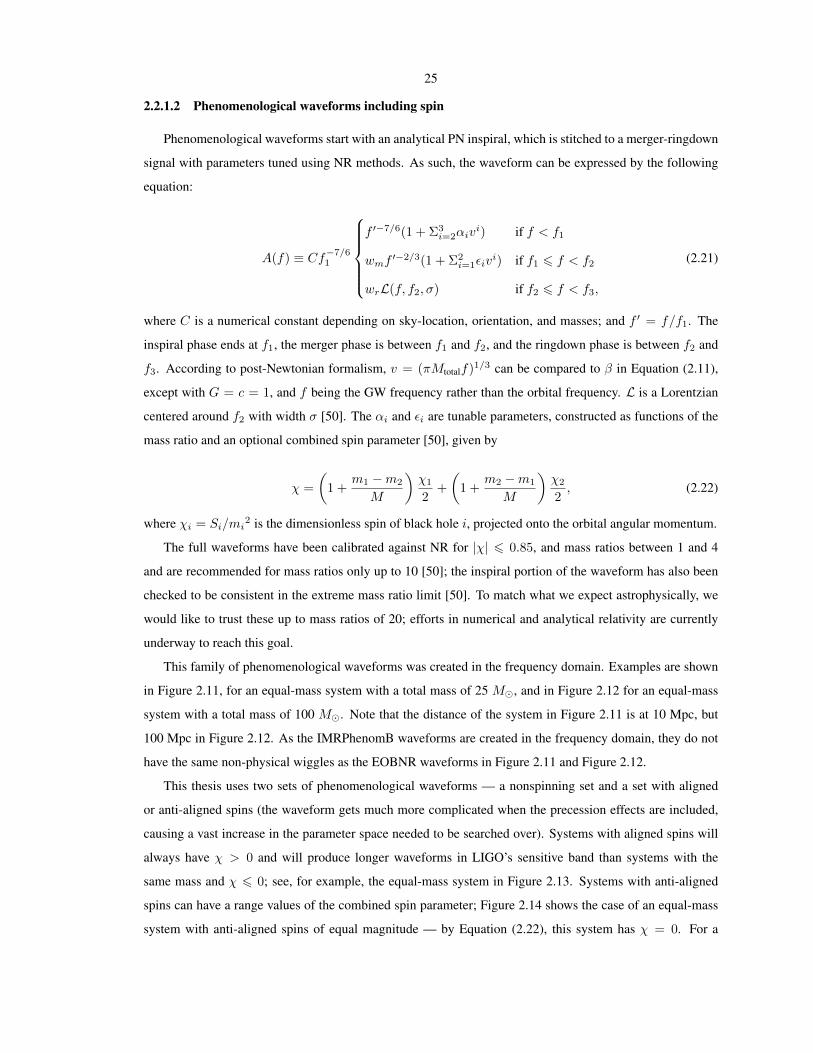
2.2.1.2 Phenomenological waveforms including spin

Phenomenological waveforms start with an analytical PN inspiral, which is stitched to a merger-ringdown

signal with parameters tuned using NR methods. As such, the waveform can be expressed by the following

equation:

A(f) ≡ Cf−7/61

f ′−7/6(1 + Σ3i=2αiv

i) if f < f1

wmf′−2/3(1 + Σ2

i=1εivi) if f1 6 f < f2

wrL(f, f2, σ) if f2 6 f < f3,

(2.21)

where C is a numerical constant depending on sky-location, orientation, and masses; and f ′ = f/f1. The

inspiral phase ends at f1, the merger phase is between f1 and f2, and the ringdown phase is between f2 and

f3. According to post-Newtonian formalism, v = (πMtotalf)1/3 can be compared to β in Equation (2.11),

except with G = c = 1, and f being the GW frequency rather than the orbital frequency. L is a Lorentzian

centered around f2 with width σ [50]. The αi and εi are tunable parameters, constructed as functions of the

mass ratio and an optional combined spin parameter [50], given by

χ =

(1 +

m1 −m2

M

)χ1

2+

(1 +

m2 −m1

M

)χ2

2, (2.22)

where χi = Si/mi2 is the dimensionless spin of black hole i, projected onto the orbital angular momentum.

The full waveforms have been calibrated against NR for |χ| 6 0.85, and mass ratios between 1 and 4

and are recommended for mass ratios only up to 10 [50]; the inspiral portion of the waveform has also been

checked to be consistent in the extreme mass ratio limit [50]. To match what we expect astrophysically, we

would like to trust these up to mass ratios of 20; efforts in numerical and analytical relativity are currently

underway to reach this goal.

This family of phenomenological waveforms was created in the frequency domain. Examples are shown

in Figure 2.11, for an equal-mass system with a total mass of 25 M�, and in Figure 2.12 for an equal-mass

system with a total mass of 100 M�. Note that the distance of the system in Figure 2.11 is at 10 Mpc, but

100 Mpc in Figure 2.12. As the IMRPhenomB waveforms are created in the frequency domain, they do not

have the same non-physical wiggles as the EOBNR waveforms in Figure 2.11 and Figure 2.12.

This thesis uses two sets of phenomenological waveforms — a nonspinning set and a set with aligned

or anti-aligned spins (the waveform gets much more complicated when the precession effects are included,

causing a vast increase in the parameter space needed to be searched over). Systems with aligned spins will

always have χ > 0 and will produce longer waveforms in LIGO’s sensitive band than systems with the

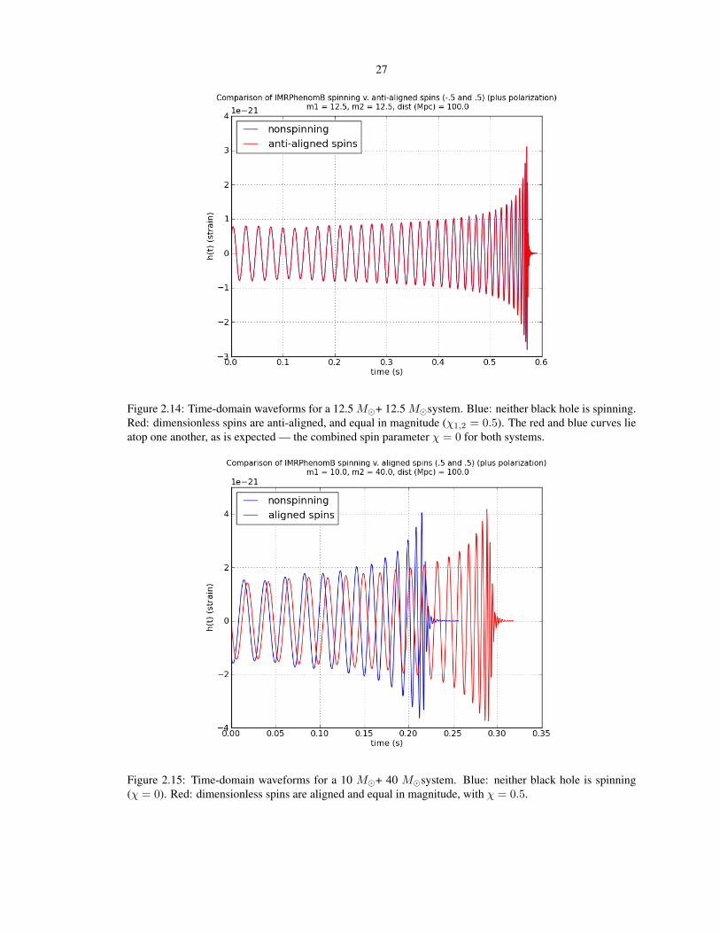
same mass and χ 6 0; see, for example, the equal-mass system in Figure 2.13. Systems with anti-aligned

spins can have a range values of the combined spin parameter; Figure 2.14 shows the case of an equal-mass

system with anti-aligned spins of equal magnitude — by Equation (2.22), this system has χ = 0. For a

26

system with a component mass ratio of 1:4 and a total mass of 50 M�, Figure 2.15 depicts the χ = 0

(non-spinning) and χ = .5 (aligned spin) case. Figure 2.16 shows the anti-aligned spin cases for the same

system (χ1,2 = ±0.5); if the more massive component has the positive dimensionless spin parameter, the

combined spin parameter is positive (likewise, if the more massive component has a negative dimensionless

spin parameter, the combined spin parameter is negative). As is seen in Figure 2.15 and Figure 2.16, as the

combined spin parameter increases, so does the length of the waveform in LIGO’s sensitive band.

The χ = 0 IMRPhenomB waveforms are also compared to their EOBNRv2 counterparts in Figure 2.7 and

Figure 2.8. Although the two models used in the analysis described in this thesis are supposed to be similar,

they differ in end time and phase evolution, which can make a big difference; therefore, it is important to

use both — until we detect GWs, we do not know which one better matches reality. The IMRPhenomB

waveforms, which are used in this thesis to assess our sensitivity, are not used in the official rate upper limit

calculation as they are not trusted above a mass ratio of 10.

Figure 2.13: Time-domain waveforms for a 12.5 M�+ 12.5 M�system. Blue: neither black hole is spinning.Red: dimensionless spins are aligned but unequal in magnitude (χ1 = 0.85, χ2 = 0.5), giving a combinedspin parameter of χ = 0.675.

27

Figure 2.14: Time-domain waveforms for a 12.5 M�+ 12.5 M�system. Blue: neither black hole is spinning.Red: dimensionless spins are anti-aligned, and equal in magnitude (χ1,2 = 0.5). The red and blue curves lieatop one another, as is expected — the combined spin parameter χ = 0 for both systems.

Figure 2.15: Time-domain waveforms for a 10 M�+ 40 M�system. Blue: neither black hole is spinning(χ = 0). Red: dimensionless spins are aligned and equal in magnitude, with χ = 0.5.

28

Figure 2.16: Time-domain waveforms for a 10 M�+ 40 M�system. Both waveforms are from systems withcomponent black holes having anti-aligned spins. Blue: a 10 M� black hole with χ1 = −0.5 with a 40 M�black hole with χ2 = 0.5, giving a combined spin parameter of χ = 0.3. Red: a 10 M� black hole withχ1 = 0.5 with a 40 M� black hole with χ2 = −0.5, giving a combined spin parameter of χ = −0.3.

Table 2.2: The number of full cycles in LIGO’s band for various non-spinning waveforms at the cor-ners of our search space. The starting frequency is of 40 Hz for the LIGO detectors. Cycles arelisted for the inspiral-only portion of the waveform (TaylorT3 at 2 PPN), the full IMR waveformin the EOBNRv2 implementation, and the full IMR waveform in the IMRPhenomB implementation.

Component masses inspiral-only(PPN)

EOBNRv2 IMRPhenomB

12.5 M�+ 12.5 M� 36 46 4824 M�+ 1 M� 219 204 23199 M�+ 1 M� 0 12 38

50 M�+ 50 M� 0 12 2

Table 2.3: High frequency cutoff, duration, and number of cycles in the detector’s bandof the different waveforms. The PPN inspiral column is taken from the 2nd PPN or-der of the inspiral (parametrized by the TaylorT4 family), which is taken to end at the in-nermost stable circular orbit. Because of design differences between the detectors, LIGOhas a low frequency cutoff of 40 Hz while Virgo has a low frequency cutoff of 30 Hz.

Component masses high fre-quency cutoff

LIGO: dura-tion (numberof cycles) inPPN inspiral

Virgo: dura-tion (numberof cycles) inPPN inspiral

12.5 M�+ 12.5 M� 175 Hz .6 s (36.1) 1.4 s (61.8)24 M�+ 1 M� 157 Hz 3.8 s (219) 8.5 s (380)99 M�+ 1 M� 38 Hz 0.6 (0) 1.7 s (46.8)

50 M�+ 50 M� 44 Hz .003 s (.5) .009 s (2.6)

29

2.2.2 The sensitivity of the detectors to compact binary coalescences

The data used in this thesis were taken from LIGO’s 6th science run (S6) and Virgo’s 2nd and 3rd science

runs (VSR2 and VSR3). By this time, the performance of the detectors was near optimal, given the design of

the instruments.

The performance of a LIGO or Virgo detector, in terms of CBC searches, is defined by the horizon

distance, which is the distance out to which it can see an optimally oriented binary (ι = 0) with an average

SNR of ρ=8, given by

〈ρ〉 =

√4

∫ fhigh

flow

|h(f)|2Sn(f)

df, (2.23)

where flow is the low-frequency cutoff determined by the detector, 40 Hz for LIGO detectors during S6

and 30 Hz for Virgo during VSR2 and VSR3; fhigh is determined by the sampling rate of the data, whose

Nyquist frequency is 1024 Hz, and the expected waveform, h(f); and Sn(f) is the power spectral density

of the detector, which is a measure of the mean square noise fluctuations [4]. It is the square of the strain

amplitude sensitivity, shown for the different detectors in Figure 2.17 and Figure 2.18.

By inserting Equation (2.19) and Equation (2.20) into Equation (2.23), setting 〈ρ〉 = 8 (a good approx-

imation to the single-detector SNR threshold for confident detection), we can solve for r = D, the horizon

distance (for an inspiral only waveform, under the quadrupole approximation):

D =1

8

(5π

24c3

)1/2

(GM)5/6π−7/6

√4

∫ fhigh

flow

f−7/3

Sn(f)df, (2.24)

which shows how the sensitivity is dependent on the chirp massM of the system. However, it is important to

note that this calculation has only taken the inspiral portion of the waveform into consideration. The merger

and ringdown can comprise a significant fraction of the power output of a GW for high-mass systems; see

how much higher above the noise the merger and ringdown are for the 100 total M� system in Figure 2.12 as

compared to the 25 totalM� system in Figure 2.11. But it is difficult to show the horizon distance analytically

for IMR waveforms because they have complicated parameterizations, numerical solutions to differential

equations, or numerical solutions to the full GR equations. Figure 2.19 uses full IMR waveforms and a

numerical analysis to illustrate how the detectors are sensitive to higher mass systems to larger distances [4].

The sensitivity of a detector is related to the horizon distance by

sensitivity (range) = D/2.26, (2.25)

since the horizon distance was calculated for a binary with optimal orientation and sky location. The factor

of 2.26 comes from integrating over sky location and inclination angles that would give an SNR of 8 (see

30

Section 3.2 for the definition of these angles with respect to a detector).

Figure 2.17: Representative curves for the strain amplitude sensitivity for LIGO Livingston (L1), in solid red,and LIGO Hanford (H1), in green, during S6 as compared to S5 (dotted lines). Note that S6 performanceexceeded the Science Requirements Document (SRD) for Initial LIGO, due to enhancements made betweenS5 and S6. The distances in the legend are the horizon distance for an optimally oriented NS+NS inspiral.Image courtesy of John Zweizig.

31The characterization of Virgo data and its impact on gravitational-wave searches. 13

Figure 2. (a) Typical sensitivity vs. frequency curves for the first three Virgo

science runs: VSR1 (2007), VSR2 (2009) and VSR3 (2010). (b) The measured VSR2

sensitivity curve is compared to the predicted noise budget [44]. The agreement

between the measured and the predicted sensitivity was the best for VSR2. For

VSR1&3 the agreement was not as good, especially at low frequency.

disturbances coupling through the mirror magnets. At high frequencies (above 300 Hz)

the sensitivity is primarily limited by the shot noise of the main laser beam and by

laser frequency noise. The frequency noise originates from the shot noise of the sensor

delivering the error signal used in the laser frequency stabilization. For intermediate

frequencies (between 100 Hz and 300 Hz), both thermal noise and shot noise limit the

sensitivity. Noise structures around 165 Hz and 210 Hz are suspected to originate from

scattered light (see section 4.2.6).

In addition to achieving a good sensitivity, it is also important to maintain the

detector in operation as long as possible in order to maximize the live-time (or duty

cycle). A lock acquisition scheme [42, 43] was designed to bring and maintain the Virgo

detector to its working point. The Virgo locking procedure has proved to be very e!cient

and robust. The lock can last for several hours or days at a time (see table 1). If lock

is lost, it can be recovered in a few minutes. When locked, the detector is manually

set in science mode when a stable state is reached. When in science mode, no external

input or detector tuning is allowed. Science mode ends when decided by the detector

operator (for maintenance or tuning) or whenever an instability causes loss of lock of

the interferometer. The beginning and the end of a lock segment are considered unsafe

in terms of data quality. Thus, the first 300 seconds after the end of locking procedure

and the 10 seconds of data before the loss of lock are, a priori, rejected and not used

for science analysis.

The first Virgo science run, VSR1, took place between May and October 2007,

in coincidence with the LIGO detectors. The second run, VSR2, started in July 2009

after a commissioning period devoted to detector upgrades. These upgrades included:

more powerful and less noisy read-out and control electronics, a new laser amplifier

that provided an increase of the laser power from 17 to 25 W at the input port of

Figure 2.18: Representative curves for the strain amplitude sensitivity for Virgo during Virgo science run(VSR) 1, 2, and 3 [5]. Note that VSR1 was during S5, while VSR2 and VSR3 were during S6.

30 40 50 60 70 80 90 100

Binary total mass (M�)

0

100

200

300

400

500

600

700

800

Hor

izon

dis

tan

ce(M

pc)

S6, H1

S6, L1

VSR2, V1

VSR3, V1

Figure 2.19: Horizon distances for non-spinning equal-mass IMR signals in the LIGO and Virgo detectors,using EOBNRv2 waveforms, which are explained in Section 2.2.1.1 as the signal model, averaged overperiods of data when the detector sensitivities were near optimal for S6 and VSR2/3, respectively [4]. Notethat above 100 M�, the horizon distance drops abruptly, as the number of cycles in the detectors’ sensitivebands go to zero (see Table 2.2).

32

Chapter 3

Ground-based interferometric GWdetection

Initial LIGO and Virgo (V1) operated between 1999 and 2010 and collected data in a series of observa-

tional science runs, delimited by commissioning breaks and hardware upgrades. Initial LIGO science data

sets are labeled science run 1 (S1), S2, S3, S4, S5, and S6; initial Virgo’s are labeled VSR1, VSR2, and

VSR3. From S1 to S5, there were three LIGO detectors, a 4-kilometer arm detector in Livingston (L1) (see

Figure 3.1), a 4-kilometer arm detector in Hanford (H1), and a 2-kilometer arm detector (H2) sharing the

same vacuum system as H1 (see Figure 3.2). H1 and L1 were upgraded for S6 [51], also known as enhanced

LIGO, to include DC readout [10], a higher powered laser, a substantially upgraded thermal compensation

system (TCS) [52] [53], and, most notably, improved sensitivity with respect to S5 for signals above 300

Hz [54]; H2 was not in use during S6. S5 (during which LIGO reached its design sensitivity [42]) and S6

have the longest stretches of science data for LIGO detectors. Some of the many papers published on the

search for CBCs from this data (and in some cases Virgo data) are References [55], [56], [23], [57], [58],

and [17]. No GWs were found, but this was not unexpected.

Currently, the H1 and L1 detectors are being replaced by their advanced versions, as is Virgo (the sites

and vacuum enclosures remain the same, but the detectors themselves are completely redesigned) [59]. We

can also look forward to LIGO-India, which will employ the base hardware from H2, and Japan’s Kamioka

Gravitational Wave Detector (KAGRA) [60], which will be underground and have cryogenically cooled test

masses.

This thesis is based mainly on the data during LIGO’s S6 and Virgo’s VSR2 and VSR3 data sets. In the

following sections I will explain the basic elements of the detectors that are required to understand the results

presented in this thesis.

33

Figure 3.1: An arial view of LIGO Livingston (L1) showing the full y-arm, part of the x-arm and the exteriorbuilding around the control room and laser and vacuum equipment area. Image taken from www.ligo.org.

Figure 3.2: An arial view of LIGO Hanford (H1 and H2) showing the full y-arm, part of the x-arm andthe exterior building around the control room and laser and vacuum equipment area. Image taken fromwww.ligo.org.

34

3.1 The operating principles of ground-based interferometric GW de-

tectors

As hinted at in Section 2.2.1, in order to detect GWs you need an instrument that measures differential

strain. Strain is equal to the change in length over length,

h = δL/L, (3.1)

where L is the length of your measuring device. A gravitational wave from a 50+50 M� system at 100 Mpc

will impart a strain on the order of 10−20 around merger (see Figure 2.12, noting that the y-axis is the strain

scaled by the square root of the x-axis). Therefore, we need an instrument that can measure very small ratios

of change in length to length.

The designers of the LIGO and Virgo detectors chose a Michelson interferometer as the basic structure for

the instrument, since it can measure small length changes δL to very high precision. In a classic Michelson,

coherent incident light is directed at a beam splitter, which sends half of the light down the x-axis and half

of the light down the y-axis. There are mirrors at the end of each arm that send the light back toward the

beam splitter (see Figure 3.3); depending on the difference in arm lengths, when this light recombines it will

either head back toward the laser (symmetric port) or toward a photodetector (anti-symmetric port). If the

arms are exactly the same length, no light hits the photodetector and thus the anti-symmetric port has earned

the nickname “the dark port”. If a GW passes through the detector, it changes the relative positions of the

mirrors, allowing a pattern of light to reach the anti-symmetric port’s photodetector — this can be calibrated

into the likely GW strain signal.

In reality, the LIGO and Virgo detectors are much more than Michelsons. The full optical configuration

is sometimes referred to as a power-recycled Fabry-Perot Michelson interferometer (PRFPMI) [61]. Fabry-

Perot and power-recycling optical cavities increase the laser power in the arms, effectively increasing L

because the light bounces back and forth hundreds of times before exiting to the anti-symmetric port, thus

improving the sensitivity at relevant frequencies by two orders of magnitude [62]. However, this signal is still

very tiny — only quadratically proportional to the small GW signal we are trying to detect. Therefore, LIGO

detectors employ either heterodyne detection (S1 - S5) or a specialized form of homodyne detection (S6)

known as DC readout. DC readout adds a local oscillator field at the same frequency as the input laser. When

a GW signal modulates the phase of the input laser, it will interfere with the local oscillator to produce power

variations on the anti-symmetric port’s photodetector that are linearly proportional to the GW signal [10].

Homodyne detection benefits from a local oscillator field that has been filtered by the Fabry-Perot arms, and

an output mode cleaner (between the beam splitter and the anti-symmetric port) which removes “junk” light

that may be resonating in the power-recycling cavity [10]. Virgo does the same thing [63].

Since the detectors are measuring extremely tiny distances with lasers, it is important that the laser light

35LIGO Detector Characterization in S6 3

Figure 1: Optical layout of the LIGO interferometers during S6 [21]. The layout differsfrom that used in S5 with the addition of the output mode cleaner.

components for the aLIGO laser system [26]. In order to correct for the higher thermallensing of the test masses [27], a improved CO2-laser thermal-compensation systemwas installed [28, 29] and used to heat the outer annulus of the input test masses tocounteract excessive lensing from the main beam.

An alternative GW detection system was installed, replacing the initialheterodyne readout scheme [30]. A special form of homodyne detection, known as DCreadout, was implemented, whereby a local oscillator field is introduced at the samefrequency as the main laser beam [31]. In this system, GW-induced phase modulationsinterfere with this field to produce power variations on the output photodiode, withoutthe need for demodulating the output signal. In order to improve the quality of thelight incident on the output photodiode in this new readout system, an output modecleaner (OMC) cavity was installed to filter out the higher-order mode content of theoutput beam [32]. The OMC was required to be in-vacuum, but also highly stable,and so a new single-stage seismic isolation system was designed and installed for theoutput optical platform [33], from which the OMC was suspended .

Futhermore, controls for seismic feed-forward to a hydraulic actuation systemwere implemented at LLO to combat the higher level of seismic noise at that site [34].This system, to be installed on all chambers at both sites for aLIGO, uses signals fromseismometers at the Michelson vertex, and at ends of each of the arms, to suppressthe effect of low-frequency (below ∼ 10 Hz) seismic motion on the instrument.

Figure 3.3: A basic illustration of a LIGO detector and its main components during S6 [6].

is extremely stable and that scattering is minimized. The beam path and optical components are enclosed in a

vacuum (10−9 - 10−8 torr for LIGO detectors) [62] so that the laser beam experiences minimal random phase

fluctuations due to residual gas fluctuations in the beampipe. Also, high vacuum ensures the mirrors do not

get dusty; dust not only causes scatter but also causes the optics to heat up unevenly [64]. The mirrors, often

referred to as test masses, are coated with dielectric and polished to have very low absorption (a few parts-

per-million (ppm)) and scattering (60− 70 ppm)) [62]. Scattering not only leads to loss in laser power where

it is needed, but to photons with the wrong frequency sneaking into the anti-symmetric port’s photodiode.

In order for Earthly motions to not influence the test masses and mimic GWs, seismic isolation systems are

used. For Initial LIGO, a passive form of isolation for components inside the vacuum is achieved by a stack of

masses and springs, providing vertical isolation at frequencies above a few Hz. This is essentially a cascade

of harmonic oscillators [65], which are natural passive mechanical low-pass filters. In addition, the mirrors

are suspended with thin wires as pendula, which further provide passive isolation in the horizontal (beam

path) direction from seismic noise as well as thermal noise coming from the passive isolation stack [65].

There are also active isolation measures taken to isolate motions in the direction of the laser beam [66].

Because Livingston experiences more seismic disturbance than Hanford (logging and other anthropogenic

activity prevented science data from being taken for most of the daytime hours prior to S4 [67] [68]), hydraulic

external pre-isolators (HEPI) that were planned as an upgrade for Advanced LIGO were added to L1 between

S3 and S4 to actively suppress vibrations [9]. In the middle of S6, the performance of HEPI was greatly

improved by adding feed-forward control; this can be seen by contrasting the sporadicity of the green dots

in Figure 3.4 from about 80 days to 156 days to the density of green dots from 156 days onward, indicating

that the detector was able to stay in lock for longer [6]. The feed-forward system “damps low-frequency

36

noise by using signals from the onsite seismometers to control movement of the vacuum chambers for the

end test masses” [66]. Hanford has been using a piezoelectric pre-isolation (PEPI) system since S2, but will

be upgraded to HEPI for Advanced LIGO [66].

LIGO Detector Characterization in S6 6

102 103

Frequency (Hz)

10−23

10−22

10−21

10−20

10−19

Str

ain

amplit

ude

spec

tral

den

sity

(1/√

Hz)

H1

L1

Figure 3: Representative strain amplitude sensitivity of the LIGO detectors during S6.

0 100 200 300 400Time (days) since the start of S6

4

6

8

10

12

14

16

18

20

22

Insp

iral

det

ecti

onra

nge

(Mpc)

H1

L1

Figure 4: The inspiral detection range of the LIGO detectors throughout S6 to anoptimally oriented and located binary neutron star merger. The rapidimprovements between epochs can be attributed to hardware and controlchanges implemented during commissioning periods.

Figure 3.4: The range (See Equation (2.25) to which the LIGO detectors are sensitive to a binary neutronstar inspiral signal, shown to illustrate the changing sensitivity as various hardware or software upgrades aremade throughout the course of the run [6].

A very important part of the detectors’ proper function are servos, also known as control loops. These

stabilize the laser amplitude and frequency at the pre-stabilized laser table (PSL), damp the pendulum motion

of the suspended optics, control the lengths of various cavities and the angular positions of the optics, and

more. For example, the lengths of the two Fabry-Perot cavities in the arms and the power-recycling cavity

are kept at an integer number of wavelengths so that new light that enters interferes constructively with the

light already resonant in the cavities. There is also a servo that controls the Michelson phase so that the

anti-symmetric port stays at the dark fringe [62]. The detector strain signal is derived from the sensing and

actuation signals of the differential arm motion control loop — see Section 3.3 below.

Virgo detectors operate in a similar fashion; see Reference [63].

3.1.1 Subsystems of the LIGO interferometers

The LIGO and Virgo detectors can be thought of as the assemblage of many subsystems. Not only does

each subsystem have a valuable role in the operation of the detector, they also provide key information in data

quality and detector characterization studies (see Chapter 4). For enhanced LIGO, the subsystems are listed

below:

• PSL: The pre-stabilized laser subsystem ensures that the laser entering the vacuum system has a stable

frequency and intensity. Additional intensity stabilization at the laser’s fundamental mode is provided

by a mode cleaner (the pre-mode cleaner) [69].

37

• IO: The input optics subsystem shares an optical table with the PSL subsystem. This subsystem’s

components (see Figure 3.5) are responsible for additional mode matching and controlling the power

and frequency of the laser that enters the interferometer. It uses an electro-optic modulator to phase

modulate the beam to produce radio frequency (RF) sidebands, which are sent into the interferometer

and to the length and alignment control subsystems [7]. The input mode cleaner is used to further

stabilize the laser frequency, and further define the transverse mode of the beam before entering the

main interferometer. Moreover, the Faraday isolator prevents light from back-scattering into the PSL

subsystem. The mode matching telescope widens the diameter of the laser while further stabilizing the

frequency and isolating the TEM00 mode that will be resonant between the ITMs and ETMs [7].

• COC: The core optics components subsystem consist of the two input test masses, the two end test

masses, the beam splitter, and the recycling mirror [69]. The optics are made from fused silica and

have specialized reflective and anti-reflective coatings applied [70].

• COS: The core optics support subsystem generates optical pick-off beams from each of the core optics

and takes them outside of the vacuum so they can be used by the LSC and ASC subsystems [71].

• SUS: The suspensions subsystem controls the position of the suspended optics (input test masses,

end test masses, and mode cleaner optics). These optics are suspended via a single wire that loops

around the barrel of the mirror. The optics have four magnets glued to them. These magnets are used

in conjunction with optical sensor and electro-magnetic (OSEM) actuators to adjust the angular and

horizontal positions of the mirrors. Once the interferometer is in lock, SUS is only used to damp

pendulum motion of the optics; length control is left to the LSC subsystem, and angular control is left

to the ASC subsystem [8].

• LSC: The length-sensing and control subsystem receives length-sensing information from the photo-

diodes and sends them to the actuators (OSEMs) on the suspensions, which adjust the longitudinal

distances between the input and end test masses (ITMs and ETMs) such that the fundamental mode

fulfills the required interference conditions. The common arm (CARM) signal is fed back to the ETMs

at low frequency and to the frequency stabilization servo at high frequencies. Servo filters process

these signals to keep stable feedback control of the loop [72]. This is the subsystem that measures and

controls DARM (the error signal that is converted into a GW signal; see the following section). This

subsystem operates at 16348 samples/second [8].

• ASC: The alignment-sensing and control subsystem has two main parts: 1) the initial alignment-

sensing (IAS) of the optics to configure them such that lock is possible by interfacing with the COC,

COS, SUS, SEI, and IOO subsystems; 2) ASC of the cavities via wavefront sensors and OSEM ac-

tuation [73]. This second part (sometimes referred to as angular-sensing and control) tracks and fixes

the pitch and yaw of 8 mirrors (beam splitter, ETMX, ETMY, ITMX, ITMY, two mode matching

38

telescopes, and recycling mirror) such that there is maximal power buildup in the Fabry-Perot cavi-

ties. Wavefront sensors, quadrant photodiodes, and a camera are used to examine the laser light and

its sidebands. See Figure 3.6 for the locations of these components. This information is fed into

a control loop that controls the mirrors’ positions via the OSEMs. Wavefront sensors are quadrant

photodiodes equipped with RF electronics; they use the Pound-Drever-Hall method to produce error

signals for the control loop. Each wavefront sensor produces two channels — the in-phase and quad-

phase demodulation of the input beam with the RF sidebands. The ASC subsystem operates at 2048

samples/second [8].

• PEM: The physical environmental monitors subsystem is composed of numerous seismometers, mag-

netometers, accelerometers, weather stations, mains voltage monitors, temperature sensors, and an

AOR radio receiver distributed throughout each LIGO site. See Figure 3.7 for the locations of these

monitors [74]. Most of these sensors are passively recording information about the state of the envi-

ronment, and are used later to assess data quality. The seismometer information, however, is used in

the seismic isolation subsystem.

• SEI: The seismic isolation subsystem uses information from the network of seismometers to actively

subtract seismic noise from the tables holding the optics. Figure 3.8 shows a seismic isolation config-

uration. The configuration includes four passive isolation stacks for each core optic, but these are not

controlled by a servo. In S6, the active isolation comes from the sensor and actuator (hydraulic external

pre-isolator for L1 and piezoelectric pre-isolator for H1). The control loop in L1 began using Weiner

feed-forward filtering in the middle of S6 [9].

• OMC: The output mode cleaner subsystem was added during S6 to support the new DC readout plan.

This subsystem removes any spurious higher-order modes that have arisen while the laser is in the

interferometer arms. The OMC also removes the RF sidebands, as they are no longer necessary (and,

in fact, add extra noise) for DC readout using homodyne detection. The subsystem includes several

optics for beam alignment and purification, as well as photodiodes for readout; see Figure 3.9 for the

locations of these components. One of the optics is outfitted with a piezoelectric actuator (for fast

position correction) and another with a thermal actuator (for slow position correction). The OMC has

its own vacuum and seismic isolation system, consisting of two active pendula mounted on an active

isolator [10].

• TCS: The thermal compensation system, upgraded during S6, corrects for under- or over-heating of the

ITMs so that their effective radius of curvature is close to the design value (otherwise the light coming

back through the ITMs will not be reflected by the recycling mirror, leading to a loss of laser power).

The subsystem includes optics, a camera for each ITM, an optical imaging system, a servo, and a CO2

laser for applying the heat [52].

39

• CDS: The control and data system provides the closed loop control of the instruments’ servos. It

is responsible for monitoring and control of the vacuum system, providing diagnostics to monitor

interferometer performance, collaborate with the PSL, ASC, SUS, LSC, and SEI subsystems. It is also

responsible for bringing the interferometer into “lock” [69].

• DAQ: The data acquisition subsystem records both digital and analog information from all the subsys-

tems’ various sensors. The amount of data can be up to 5 Mbytes per second during S6 (this number

will increase by an order of magnitude for Advanced LIGO) [69].

These subsystems are responsible for getting the detector into lock (i.e., the fundamental mode of the laser

is resonant in the Fabry-Perot cavities, and the mirror positions are stable), keeping the detector under length

and alignment control at its design configuration, and recording information from the various components

of the detector. Each time-varying piece of information is recorded in a data channel. Data channels are

described in the following subsection.

Figure 3.5: An illustration of the input optics subsystem for LIGO during S6 (enhanced LIGO). The electro-optic modulator produces the RF sidebands that are used by other subsystems; this is the last componentthat is outside the vacuum. The mode cleaner suppresses laser light that is not in the TEM00 mode, providesfrequency stabilization, and passively reduces beam jitter above 10 Hz. The Faraday isolator prevents back-propagation of the laser and provides access to the symmetric port beam for length and alignment-sensing [7].

3.1.2 Data channels

In the language used by the LVC, data channels refer to streams of digital numbers, sampled at several

fixed frequencies, from different components of the detectors. In general, these are time-series taken by

measurement devices or used by servos at various sampling rates.

The main output of an interferometric gravitational wave detector is, of course, the signal measured by the

photodetector at the anti-symmetric port; this differential arm length (DARM) information is recorded in the

GW channel. But the GW channel is just one of the tens of thousands of channels located on and around the

detectors. The other channels are known as auxiliary channels. In addition to being used by the subsystems

listed in the previous section, they monitor two main sources of noise: instrumental and environmental.

Many of the instrumental channels record information from the servos controlling the laser and the position

40

Figure 3.6: An illustration of the angular-sensing and control subsystem for LIGO during S6 (enhancedLIGO). The QPDs (quadrant photodiodes) sense the alignment of the light transmitted to the ETMs (endtest masses). The WFSs (wavefront sensors) sense the angular alignment of the input beams with respect totheir resonant cavity modes. The camera senses the beam position incident on the BS (beam splitter). Thepositions of the ETMs, BS, ITMs (input test masses), RM (recycling mirror), and MMTs (mode matchingtelescopes) are adjusted with OSEMs via a servo using the information from the QPDs and WFSs. [8]

and alignment of the optics [75]. Figure 3.10 shows some of the devices used for recording information from

the optics. In addition to instrumental channels, there are physical environmental monitor (PEM) channels

that collect data from numerous places along the detector, recording seismic, acoustic, electromagnetic, etc.

information [75] (see Figure 3.7).

These channels can be monitored to inform scientists when an individual subsystem or the detector as a

whole is functioning properly or not. When they are not, or when a short-duration instrumental or environ-

mental disturbance occurs, a signal can be seen in the GW channel that is not due to a GW; for example,

seismic motion moves the mirrors and scattered light can hit the photodetector. Thus, the auxiliary chan-

nels can be used to veto data that is untrustworthy [76] (as discussed in Chapter 4) or to create a ranking

system that indicates the level of trustworthiness of the data (see Chapter 6). Table 3.1 lists some of the

most important channels used in the detector characterization and data-quality studies described in detail in

Section 4.1.3.

3.2 Antenna response of detector to GW signals

The strain seen by an interferometric GW detector depends on the orientation of the detector with respect

to the source as well as the polarization of the incoming GWs. The following equation projects the effect of

the different polarizations onto the plane of the detector:

h(t+ t0) = F+(θ, φ, ψ, t+ t0)h+(ι,Σ, t+ tc) + F×(θ, φ, ψ, t+ t0)h×(ι,Σ, t+ tc), (3.2)

41

Table 3.1: A non-comprehensive list of various auxiliary channels recorded by components in the LIGO de-tectors

Channel name DescriptionLSC-{MICH,PRC,DARM,CARM} CTRL 16384-Hz channels recording the information used to control

the Michelson, power-recycling cavity, and differential andcommon arm length degrees of freedom.

LSC-DARM ERR A 16384-Hz channel recording the error signal for the con-trol loop associated with the GW signal and described in Sec-tion 3.3.

LSC-REFL {I,Q} 8192- (in-phase) and 4096- (quad-phase) Hz channels moni-toring the light coming back through the symmetric port, mea-sured by RF photodiodes in the Faraday isolator. See Fig-ure 3.10.

ASC-{E,I}TM{X,Y} {P,Y} 512-Hz angular torque feedback control signals for pitch andyaw of the X and Y ETMs and ITMs.

ASC-QPD{X,Y} {P,Y} 256-Hz channels measuring the beam position on the X and YETMs.

ASC-WFS{1,2,3,4} {Q,I} {P,Y} 512-Hz channels measuring the in-phase and quadrature read-out of the alignment of the beam with respect to detector’s cav-ities. How the WFSs align to the different optical cavities isbeyond the scope of this thesis.

OMC-QPD{1,2,3,4} {P,Y,SUM} OUT DAQ 4096-Hz (for QPD{1,2} and 2048-Hz (for QPD{3,4}) chan-nels measuring the pitch, yaw, and sum motion of the OMCmirrors. The pitch, yaw, and sum can be derived from the fourquadrants of the photodiode: PITCH = (UL+UR)-(LL+LR),YAW = (UL+LL)-(UR+LR), SUM = (UL+UR+LL+LR);where the quadrants are labeled by upper, lower, left, and right.

PEM-E{X,Y} SEIS{X,Y,Z} 256-Hz channels recording seismic activity in the X,Y, and Zdirections at the X and Y end stations.

PEM-LVEA MAG{X,Y,Z} 2048-Hz channels recording magnetic fields in the X, Y, and Zdirections in the laser and vacuum enclosure area at the vertexof the interferometer.

PEM-RADIO LVEA 2048-Hz channels recording information from a radio receiverin the laser and vacuum enclosure area at the vertex of the in-terferometer.

PEM-{PSL1,BSC1,BSC3,HAM3,HAM6,LVEA,ISCT} MIC 2048-Hz channels recording audio noise in various placesaround the detector; see Figure 3.7 for their locations, but theareas on the detector are labeled in Figure 3.10.

SEI-{ITMX,ITMY,ETMX,ETMY,BS,RM} {X,Y,Z} 256-Hz channels recording seismic activity in the X, Y, andZ directions from seismometers near various optics inside thevacuum system .

SEI-OUT {X,Y} 256-Hz channels recording the output of the control system foractive seismic isolation in the X and Y direction.

SUS-{ITMX,ITMY,ETMX,ETMY,BS,RM} SUS{PITCH,YAW} IN 64-Hz channels recording the pitch and yaw of various optics.SUS-{ITMX,ITMY,ETMX,ETMY,BS,RM} OPLEV {P,Y}ERROR 512-Hz channels containing the error signal for the SUS con-

trol system for the pitch and yaw of various optics.SUS-{ITMX,ITMY,ETMX,ETMY} {LL,LR,UL,UR}COIL OUTPUT 16 Hz channels containing the values of the currents in the

coils used to control mirror positions.

42Environmental Influences on LIGO Detectors in S6 5

Fig. 2. The Physical Environmental Monitoring system layout at the LIGO Livingstondetector during S6. The setup for LIGO Hanford was very similar. Shaded regions indicatethe vacuum enclosure. Circles and rectangles indicate vacuum chambers where mirrors weresuspended. Optical tables were surrounded by acoustic enclosures but were not in vacuum.

Type Sensor Operating Frequency

seismometer Guralp R� 0.1-20 Hzaccelerometer Wilcoxon R� 731-207 1-900 Hzmicrophone Bruel&Kjaer R� 4130 15-900 Hz

magnetometer Bartington R� 03CES100 0-900 Hzradio station AOR R� AR5000A tunable

Table 1. The more important PEM sensor types and the frequency ranges in whichthey are used. The frequency range is a combination of sensor calibration range fromthe manufacturer and the sampling rate at which they are recorded.

Figure 3.7: A diagram depicting the locations of physical environmental sensor locations at L1. Figurecourtesy of Annamaria Effler.

where F+ and F× are the antenna pattern factors of a specific detector. They depend on time since the

detectors are on the Earth, which is rotating with respect to celestial coordinates. t0 is the average time the

coalescing signal reaches the rotating detector and tc is the time the system coalesces at the center of the Earth

(a fiducial location common to all detectors, making t0 − tc the propagation time from the detector to the

center of the Earth. Σ contains all the other parameters in the waveform (see, for example, Equation (2.16)).

In order to define the angles, we must set up three coordinate systems — see Figure 3.11. The inclination

angle ι is the polar angle between the source frame’s z-axis (for CBCs, this is the direction of the orbital

angular momentum) and the detector’s z’-axis (roughly, the local zenith). The polarization angle ψ is the

azimuthal angle from the detector’s x’-axis to the GW’s x”-axis. (Note that the terminology is a bit confusing

here — the inclination angle determines the polarization content of the GW, while the polarization angle

determines the angle between the stretch-squeeze in the h+ wave and the axes of the arms of the detector).

θ is the polar angle between the detector’s z’-axis and the GW’s z”-axis (the direction of propagation of the

GW). φ is the azimuthal angle between the x’-axis and the projection of the z”-axis onto the x’-y’ plane.

43

Figure 3.8: A representation of the seismic isolation stack for one of the suspended optics. Inside the dashedline is the vacuum system. The isolation stack provides passive isolation and the sensor and actuator are usedto provide active seismic isolation in the x- and y-directions [9].

Figure 3.9: A representation of the output mode cleaner optical setup [10].

Using these definitions, the antenna pattern factors can be expressed as [42]:

F+ =1

2(1 + cos2 θ) cos 2ϕ cos 2ψ − cos θ sin 2ϕ sin 2ψ (3.3)

and

F× =1

2(1 + cos2 θ) cos 2ϕ sin 2ψ + cos θ sin 2ϕ cos 2ψ. (3.4)

We can average over all polarization angles, since these should be independent of the direction of arrival,

44

WFS 3

WFS 4REFL 1

REFL 2

RE

FL C

AM

MC

WF

S 1

MC

WF

S 2

MC

RE

FL C

AM

WFS 2

WFS 1

ASPD 5

POX

SPOB

POBAS CAM

IFI

SM

MMT1

MMT3IMC1

IMC3IMC2

MMT2

PRM

BS

ITMX ETMX

ITMY

ETMY

QPDY

TRANS PD Y

TRANS PD X

QPDX

QPD4

QPD3

QPD2

OFI

QPD1

TT1

TT0

TT2

DCPD1DCPD2

OMC TRANS CAM

HAM 1 HAM 2 HAM 3

HAM 4

TR

GR

PD

HAM 6

BSC 1

BSC 2 BSC 3 BSC 4

BSC 5

IOT 1

ISCT 1

ISCT 4

4 km

4 km

Jeffrey S. Kissel

LIGO-G0900777-v5

Approx. Radii of Curvature (m)

MC2 17

MMT1 7

MMT2 3

MMT3 25

RM (HR) 16000

ITMs (HR) 15000

ETMs 9000

TT1 5

M2 2

M4 2

(Unspecified optics are flat)

M1

M2

M3

M4

Approx. Distances (m)

MMT1 to MMT2 14

MMT2 to MMT3 14

MMT3 to RM 16

RM to BS 4

BS to ITMs 5

ITMs to ETMs 4000

BS to TT0 24

TT0 to TT1 1

TT1 to TT2 2

TT2 to OMC 0.3

L1's Enhanced LIGO Optical Layout

Optics (Fused Silica)

Laser Light (! = 1064e-9 m)

RF Photo Diode

DC Photo Diode

Faraday Isolator

IR Camera

RF Wave Front Sensor

DC Quadrant Photodiode

Shutter

High-power Beam Dump

Important Notes- THIS DRAWING IS NOT TO SCALE, and HAM5 is not shown because it contains no optics in enhanced LIGO.

- Several important optics (specifically lenses on ISCT tables) have been left out of this diagram for simplicity.

- The optical layout of the ISCT Tables frequently changes and thus it is possible (if not probable) that their layout is only roughly correct.

- The quoted radii of curvature and distances are merely for rough scaling and are not to the accuracy needed for anything more precise than a ballpark calculation.

Light from PSL

Relevant AcronymnsHAM - Horizontal Access Module PRM (or RM) - Power Recycling MirrorBSC - Beam Splitter Chamber BS - Beam SplitterPSL - Pre-Stablized Laser ITM - Input Test MassSM - Steering Mirror ETM - End Test MassIMC (or MC) - Input Mode Cleaner BRT - Beam Reducing TelescopeMMT - Mode Matching Telescope WFS - Wave Front SensorIFI - Input Faraday Isolator AS - Anti-Symmetric portREFL - Reflected Light TRANS - Transmitted LightIOT - Input Optics Table TT - Tip Tilt (Telescope)ISCT - Interferometer Sensing and Control Table OMC - Output Mode Cleaner(S)PO(B,X) - (Sideband) Pick Off (Beamsplitter, itmX) QPD - Quad Photo Diode

BRT2

BRT1

Figure 3.10: A diagram depicting the locations of various optical components and the auxiliary channelsrecording information from/about them. Figure courtesy of Jeff Kissel.

and calculate the mean square response of the detector as

F2

=

∫F 2

+dψ =1

4(1 + cos2 θ)2 cos2 2ϕ+ cos2 θ sin2 2ϕ (3.5)

= F 2+(θ, ϕ, ψ = 0) + F 2

×(θ, ϕ, ψ = 0), (3.6)

which is visualized in Figure 3.12.

3.3 Calibration

The formulas and theory in this section are from Reference [77] and conversations with Alan Weinstein.

For LIGO detectors, calibration is the process of converting one (or more) of the data channels of

the LIGO detector into GW strain. In other words, it takes the channels LSC-DARM ERR and LSC-

DARM CTRL (see Table 3.1) and turns them into h(t). In S6, DARM ERR is constructed via DC readout;

but in S5 it was derived from LSC-AS Q (see Table 4.1).

Calibration involves understanding the frequency-dependent amplitude and phase response of each ele-

45

Figure 3.11: The relevant angles for the calculation of the strain seen by an interferometric GW detector. Thex’-y’-z’ frame is that of the detector, the x-y-z frame is that of the source, and the x”-y”-z” frame is that of theGWs. ψ is the polarization angle. The z-axis is defined by aligning it with the orbital angular momentum ofthe binary system. The z”-axis is defined by the direction from the source to the detector; the x”- and y”-axesare defined by the stretching and squeezing directions of h+ in the GW frame (see Figure 2.4). The x’- andy’-axes are defined by the arms of the detector; we then use the right hand rule to define the z’-axis [11].

ment in the DARM control loop shown in Figure 3.13. The incoming GW signal, i.e., the ∆Lext input in

the control loop, and the corresponding motion of the mirrors are analog; but the readout, eD, is measured

in digital counts proportional to mirror displacement. In the context of control loops, eD is the control loop

error signal, often referred to as DARM ERR, or the GW channel. Because C, D, and A are functions of

frequency (and γ(t) is a slowly changing function of time due to the optical gain changing from laser power

fluctuations or mirror misalignments), as we travel through the control system, we multiply their effects as

follows:

eD = γ(t)C(f)∆Lext − γ(t)C(f)A(f)D(f)eD, (3.7)

where γ(t)C(f) is the length-sensing function, A(f) is the actuation function describing how the test masses

respond to the influence of the control loop, and D(f) is the set of digital filters, which are implemented into

the LIGO control system in order to transform the error signal into a control signal, like

D(f)eD = sD, (3.8)

where sD(f) is the digital control signal. sD(f) is one of our data channels, DARM CTRL (see Sec-

46

34

Figure 9 : Level surface of the detector response function. The directions of the interferometer

arms are shown.

Figure 3.12: The root mean square antenna pattern of a LIGO detector whose x- and y-arms are representedby the black bars to circularly polarized GWs [12].

!(t) C

D!

A

eD

-1

"LA

"Lext

Analog D

igit

al

Figure 3.13: The control loop for LIGO interferometers. ∆Lext is the motion of the mirrors caused by GWsor a local disturbance, γ(t)C(f) is the length-sensing function, eD is digital error signal, D(f) is the setof digital filters on eD in order to feed it into is the actuation function A(f) that calculates the ∆LA in anattempt to cancel the ∆Lext.

tion 3.1.2), and is designed to keep DARM ERR close to zero. Similarly, the actuation function can be

expressed as

A(f)sD(f) = ∆LA, (3.9)

47

where ∆LA is corrective displacement on the mirrors exerted by the control loop.

The control loop can also be expressed by the following equation, derived from Equation (3.7):

eD =γ(t)C∆Lext

1 + γ(t)CAD=γ(t)C∆Lext

1 +G, (3.10)

where G = γ(t)CAD is known as the open loop transfer and can be split into two parts

G = γ(t)G0(f), (3.11)

where G0(f) = CAD is known as the nominal open loop transfer function. G0(f) is measured experimen-

tally by sweeping through all frequencies in a procedure known as swept sine calibration to give us G0(f) at

snapshots of time.

There are three inherent problems with this approach alone. Firstly, in between swept sine shapshots,

which are only taken a few times during each science run, there can be time variation of G(f, t). We try

to capture this time variation with γ(t), using permanent calibration lines at well-chosen frequencies around

50, 400, and 1100 Hz; the statistical error on this procedure is captured by measuring γ(t) every second

and computing the standard deviation. Secondly, the swept sine procedure itself also has statistical error,

measured by repeating the measurement. Thirdly, there is a systematic error which is estimated by comparing

a detailed theoretical model of G to our measurements.

The goal is, of course, to translate any given eD at a snapshot of time into the corresponding GW strain,

causing the mirror motion ∆Lext(f), which requires learning the form of the response function RL,

∆Lext(f) = RL(f)eD(f), (3.12)

where RL is given by

RL(f, t) =1 + γ(t)G0(f)

γ(t)C(f). (3.13)

A simple convolution uses the response function and the error signal to calculate the gravitational wave strain

in the time domain:

h(t) =1

L

∫RL(t− t′)eD(t′)dt′, (3.14)

where RL(t) are digital finite impulse response (FIR) filters calculated from RL(f).

As the open loop gain is known by measurement, all that remains to get a full model of the amplitude

and phase of RL(f, t) is to find γ(t)C. We know γ(t) by measurement, but in order to model C(f) we must

extract its contribution from G0(f) = CAD. We know D exactly by construction; we know the functional

form of the frequency response of both C (cavity pole) and A (damped, driven pendulum) by theory.

The cavity pole response function can be calculated from the knowledge that a change in the length of the

48

Fabry-Perot cavity will cause the phase of the laser light exiting the cavity to be different than when it entered

the cavity. The transfer function (on resonance) between the cavity length and the change in phase is:

HFP(f) =2π

λ

1

rc

re(1− r2i )

1− riresin(2πfL/c)

2πfL/c

e−2πifL/c

1− riree−4πifL/c, (3.15)

where rc = (re − ri)/(1 − rire) is the reflectivity of the Fabry-Perot cavity on resonance and re ∼= 1 and

ri =√

1− 0.3 are the reflectivity of the end and initial test masses, respectively. L is the length of the cavity

and c is the speed of light. The frequency dependence of this transfer function can be expressed as a simple

cavity pole response,1

1 + i ffpole

, (3.16)

where f is the frequency of the ∆Lext signal, and fpole = c(1 − rire)/2πL(1 + rire) is approximately 90

Hz for initial and enhanced LIGO detectors. This cavity pole transfer function is defined as the ratio of

Equation (3.15) at f � c/2L to it at f = 0.

The damped, driven pendulum equation can be expressed as a force-to-displacement transfer function for

the center of mass of the optic:

P ∝ 1

f20 + i f0Q f − f2

, (3.17)

where f0 is the natural frequency of the pendulum (nominally 0.74 Hz), Q is the quality factor of the pendu-

lum (10 for H1 and 100 for L1), and f is the driving frequency [77].

The challenge is to separate amplitudes of the transfer functions C and A. The separation of these

constants is accomplished with the free-swinging Michelson technique, in which the interferometer is not

under control of the control loop, the arms are not locked, and the light in the cavities is not at resonance. In

this configuration, the input test mass mirrors are moved with the actuation coils and then let go, allowing

them to swing through the Michelson fringe, which we know is exactly one wavelength of our laser (1064

nanometers). A separate procedure transfers this normalization of the calibration coefficients from the input

test masses to the end test masses by locking the arms. By also looking at eD as this happens, we can figure

out the amplitude of the actuation function A; from this the amplitude of the length-sensing function C can

be extracted as well.

Calibration is important because it is the largest known source of systematic error in the analysis described

in this thesis, as well as most analyses of LIGO data. The calibration systematic error is due to the uncertainty

in the amplitude and phase of the response function as a function of frequency of Lext. The full error analysis

can be found in Reference [77]. For the high-mass search, the other significant source of systematic errors

are from our uncertainty in our waveform models (not as quantifiable) and the Monte Carlo errors on the

software injections used to evaluate the efficiency of our pipeline (easily quantifiable).

49

3.3.1 Hardware injections

We can use the control loop described above to make the detectors behave approximately as they would

in the presence GWs. To perform one of these so-called hardware injections, we first calculate the detector

strain h(t) that would be produced by a particular astrophysical source. Using a transfer function from strain

to mirror force coil voltage counts (for f � f0):

T (f) =L

C

f2

f20

, (3.18)

where L is the length of the interferometer’s arm, C is the calibration point in nm/count, and f0 is the pen-

dulum frequency of the end test mass (0.74 Hz); we can transform h(t) into v(t). When v(t) is injected into

the control loop, an end test mass moves in approximately the way the astrophysical signal would cause it

to. Hardware injections are used to test our understanding of calibration, search algorithms (for example, the

one described in Chapter 7), and veto safety (see Section 4.2.1.5) [78].

An example of a hardware injection of a high-mass signal can be seen as a spectrogram in Figure 3.14

and as a time-series in Figure 3.15.

Figure 3.14: A whitened time-frequency spectrogram illustrating a GW signal from a 18.901 + 15.910M� system, at a distance of 19.557 Mpc, as seen in L1’s GW channel. This signal was produced via ahardware injection.

50

Figure 3.15: A raw timeseries illustrating a GW signal from a 18.901 + 15.910 M� system, at a distanceof 19.557 Mpc, as seen in in L1’s GW channel. Note, however, that the signal (the injected CBC chirpwaveform) is lost in the much larger low frequency noise. This signal was produced via a hardware injection.

3.4 LIGO and Virgo detectors’ noise

The sensitivity of interferometric GW detectors is strongly frequency-dependent due to design choices

and the physical limitations of the various components of the detectors. Depending on the noise spectra, a

detector is more or less sensitive to different astrophysical sources. Measured noise spectra can be seen for

LIGO and Virgo in Figure 2.17 and Figure 2.18, respectively. For initial LIGO, the theoretical forms of these

noise sources are shown in Figure 3.16; experimentally-derived noise curves for one of the LIGO detectors

during S6 are shown in Figure 3.17. These figures, sometimes referred to as the “noise budget”, are created

by back-referencing the noise (which can come in a variety of units) from various sources via mathematical

models used to calculate the strain equivalent noise. In other words, not all noise sources manifest as strain

noise (moving the mirrors, or changing the frequency of the laser such that it appears that the mirrors have

moved), but can be translated into displacement/strain noise by using a transfer function.

The main sources of noise are described in the following list, following Reference [13]:

• Seismic noise is due to the motion of the Earth from across the world (Earthquakes, .01 - 1 Hz), to ocean

waves shaking the continental plate that LIGO sits on (microseismic, ∼ 1/6 Hz), to wind and human-

produced noise (anthropogenic, 1 - 30 Hz). The shape of curve is due to the noise at the test mass,

after filtering by the mirror suspension and seismic isolation system (see Figure 3.8), which consists of

the active HEPI system (in L1 only), the passive three-stage seismic isolation system and the actively

51

damped single-pendulum system, each of which adds a 1/f2 reduction in the noise. Accounting for

the ground motion, which already decreases as a function of frequency, the seismic noise curve falls

rapidly above 10 Hz (more steeply than f−10.

• Thermal noise is present in any damped mechanical system, as described by the the Fluctuation-

Dissipation Theorem, which states that the damping (dissipation of thermal energy) comes along with

Brownian motion in the system’s modes of oscillation [79]. This is relevant to the pendulum-suspended

mirrors (whose fundamental mode peaks at 0.74 Hz), the violin modes of the suspension wires (mul-

tiple peaks clustering at 340 Hz and harmonics), and the drum mode of the test masses themselves

(above 10 kHz). In the pendulum, the noise falls as 1/f2 above the pendulum frequency (0.74 Hz)

and below the the violin mode resonances (which are not shown in Figure 3.16, but can be seen in Fig-

ure 3.17). In the test masses, this noise falls as 1/√f assuming a constant (independent of frequency)

mechanical loss of the mirror material, causing the noise to leak outside of the drum mode peak.

• Radiation pressure and shot noise are two sides of the coin of quantum laser noise. The shot noise is

due to quantum fluctuations in the number of photons reaching the anti-symmetric port’s photodiode.

It rises linearly with frequency due to the cavity pole transfer function (take the magnitude of Equa-

tion (3.16)) that transforms a phase shift in the light to a GW signal. Shot noise can be lowered by

increasing the power of the laser or including a power-recycling cavity. However, doing so increases

radiation pressure noise because there are more photons pushing on the mirrors, and therefore more

quantum fluctuations in the number of photons. The radiation pressure noise theoretically falls as 1/f2,

because it is just “white” force noise transformed into displacement noise as in Equation (3.17). The

radiation pressure noise increases with the intensity of the laser. The origin of these has been shown

to be the quantum noise of the vacuum entering the anti-symmetric port [80]. Shot noise dominates

the GW noise spectrum in initial LIGO from 250 Hz to 8 kHz, as is evident in Figure 3.17. Radiation

pressure noise has not been observed in LIGO; it lies below other noise sources at low frequencies,

as illustrated in Figure 3.16 and Figure 3.17. In Advanced LIGO, radiation pressure noise will be the

dominant noise source between about 10 and 40 Hz [59].

• Residual gas noise is due to gas molecules that were not eliminated during the vacuum pumping of the

instrument’s interior. This gas produces several sources of noise. First, there will be a non-unit and

fluctuating index of refraction in the beam tubes, causing phase fluctuations on the laser light (sensing

noise), which we interpret as GW strain. In addition, the residual gas will randomly kick the mirrors,

causing displacement noise; this is negligible in initial LIGO. In addition, dust particles deposited on

the mirrors produce scattering centers; the scattered light finds its way back to our detection photodiode,

producing glitches.

52

Figure 3.16: The theoretical noise sources limiting initial LIGO strain sensitivity. See Section 3.4 for adetailed description of each contribution to the noise [13].

3.4.1 Gaussian versus non-Gaussian noise

The noise curves presented in the previous section are the result of time-averaging the noise and do

not represent the non-stationarity of the noise at either long or short timescales. The long-timescale non-

stationarity is evident in the binary neutron star range as a function of time, Figure 3.4. The main sources of

short-timescale non-stationarity are laser intensity fluctuations and alignment issues, which generally mani-

fest as low-frequency non-Gaussian noise. On the other hand, the quantum noise at higher frequencies tends

53

to be more Gaussian. Here, we distinguish between two types of non-Gaussianity. The first are excursions

101 102 10310−20

10−19

10−18

10−17

10−16

10−15

Frequency [Hz]

Disp

lace

men

t [m

/!Hz

]H1 (DC) at 2010−07−21 11:50:00, (963748215)

UGF = 186Hz, Req. PWR = 20 W, range: 25.8 MPc pred, 19.2 MPc meas

crea

ted

by m

akeN

oise

Plot

on

22−J

ul−2

010

ShotDarkIntensityMICHPRCBSETMITMASCOpLevOSEMSeismicRadPressIntThermSusThermtotalnoiseSRDDARM

Figure 3.17: The noise budget for H1 during S6. The shot noise is due to the Poisson fluctuations in the laserlight hitting the anti-symmetric port’s sensing photodiode. The dark noise is the noise that is measured on thephotodetector when the laser is turned off; it is due only to the electronics themselves. The intensity noise isdue the fluctuations in the laser intensity, whose power emitted is nominally 20 W. The MICH noise is fromthe control signal that keeps the anti-symmetric port dark. Similarly, the PRC noise is from the control signalthat keeps the laser resonant in the power-recycling cavity. The BS (beam splitter), ETM (end test masses),ITM (input test masses) and ASC (angular-sensing and control) noise is residual noise from control systemsthat monitor and control the mirrors’ positions and orientations. The OpLev noise is from the optical leverservo, which senses and controls the mirror angular positions (pitch and yaw). The OSEM noise is from theoptical shadow sensor and magnetic actuator, which locally damp the pendulum motion of the mirrors. Theseismic noise is due to a variety of sources that produce displacement noise at the mirrors (ITMs and ETMs).The IntTherm noise is the thermal noise internal to the test masses themselves. The SusTherm is the thermalnoise in the suspension wires at the violin mode frequencies of 340 Hz and harmonics; it also includes thependulum mode at 0.74 Hz (off the scale of this plot) and 1/f2 falloff. The totalnoise curve is the sum ofall the listed noise sources (which were already transformed into displacement noise), added in quadrature.The DARM curve is the total noise measured at the anti-symmetric port; the gap between the DARM curveand the total noise curve, especially noticeable below 60 Hz, is not quantitatively understood. The SRD isthe strain sensitivity goal listed in the science requirements document [14], presented to the National ScienceFoundation in 1995.

54

of 3 to 5 σ from the mean. These alone are not problematic, because they are rarely found in coincidence

between detectors. The second are the extremely non-Gaussian excursions of many more σ from the mean;

these are the glitches that really limit our sensitivity because they need only be found in coincidence with a 3

σ excursion in another detector. The next chapter goes into the causes of several types of glitches, as well as

methods used to veto them.

55

Chapter 4

Glitches, their effect on data quality, andthe need for vetoes

As discussed briefly in Section 1.3, glitches are a problem for the high-mass search because they cause

events with a large signal-to-noise-ratio to be found by the matched-filter algorithm. These events not only

obscure potential astrophysical GW events, but also would lower our detection confidence in a true event.

Of course, the effect is not limited to the high-mass search; glitches present problems for every search done

by LIGO and Virgo. This chapter discusses glitches and glitch-finding algorithms in general, gives specific

examples of glitches in LIGO S6 data, and explains the traditional methods of mitigating the effect of glitches

on a search like the high-mass search. There are two main titles given to research in this realm — data quality

and detector characterization. Although much of their work overlaps, they can be distinguished by the

direction the information learned travels — data-quality information tends to go downstream to astrophysical

search pipelines, while detector characterization information tends to go upstream to detector commissioners.

4.1 Glitches and glitch-finding algorithms

Glitches are short duration events recorded by the GW channel that can be attributed to an environmental

or instrumental disturbance and, as such, we are confident they are not GWs. For the high-mass search, for

example, glitches are spurious events that are picked up by the matched-filter algorithm, which compares the

data in the GW channel to short-duration templates that model waveforms from high mass binary black hole

coalescence. Therefore, glitches with duration and frequency content comparable to the the waveforms listed

in Table 2.3 cause the most difficulty for the high-mass search, because the high-mass templates are so short

that a χ2 test does not work well (see Section 7.3.6 for an in-depth discussion of this test).

Glitches can be identified with various algorithms. Two such algorithms were used in this thesis; they

are described in the following subsections. The shared goal of these algorithms is to do a fast transform in a

wavelet basis that is essentially performing a matched-filter for shapes that look like glitches. These glitches

can be found not only in the GW channel, but also in the auxiliary channels; Figure 4.1 shows a glitch in

56

one of the auxiliary channels. Like many glitches it can be characterized as a ringdown — an abrupt change

followed by a decay described by normal modes.

Figure 4.1: An extremely loud glitch seen in an auxiliary channel recording the sum of the photode-tectors in the output mode cleaner. Image courtesy of the Detector Characterization group Wiki pagehttps://wiki.ligo.org/DetChar/OMCSpikeGlitches. Note the characteristic ringdown shape.

4.1.1 KleineWelle as a glitch-finding algorithm

In a general sense, glitches manifest as excess energy in a time-series. KleineWelle (German for ”little

wave”, or wavelet) uses the dyadic wavelet transform [81], a multiresolution technique that looks for excess

energy in the time-scale space [82]. Dyadic, here, means that the wavelet coefficients are calculated for size

scales (time-scales, for us) that vary by powers of two. KleineWelle is useful because it is able to identify and

characterize transients in any time-series, such as those from the LIGO detectors’ data acquisition systems.

A wavelet transform, as opposed to a Fourier transform, is designed to look for small bumps in the data. A

wavelet transform, much like a Fourier or Laplace transform, can be expressed as an integral

Wg(u, s) =

∫ ∞

−∞g(t)

1√s

Ψ∗(t− us

)dt, (4.1)

where g(t) is the time series; s defines the scale; Ψ is the wavelet, which is a function of t−us , where u is a

generic time variable with the same range as t. Depending on the scale, we have good time resolution at the

57

expense of frequency resolution (small scale) or good frequency resolution at the expense of time resolution

(large scale) [82]. In other words, at large frequencies, we have poor frequency resolution and good time

resolution — see Figure 4.2. Many wavelets can be used; the one currently employed by most LIGO analyses

is the Haar wavelet, which can be seen in Figure 4.3.

Figure 4.2: The tiling of time-frequency space for the KleineWelle algorithm. The central frequencies of eachtile are related by powers of 2. Scale refers to the tile width on the time-axis. The tiles at high frequencieshave small scale and poor frequency resolution. The tiles at low frequencies have high scale and poor timeresolution [15].

Figure 4.3: A plot of the Haar wavelet. As the scale increases, the wavelet widens. Image courtesy ofWikipedia.

In the case of discrete data (data channels from the LIGO data acquisition system are typically sampled at

rates that are powers of two (see, for example, the channels’ rates in Table 3.1) we can, instead of computing

the integral, use high and low pass filters. See Reference [83] for a discussion of the general computational

application of Haar wavelets.

We can define normalized tile energies (sometimes referred to as pixel energies), for each tile in the

time-frequency plane:

Ej = Y 2j /σ

2j , (4.2)

58

where the Yj are the discretized versions of the wavelet coefficientsWg(u, s). For sufficiently large j (scale=

2j), the Yj are Gaussian distributed with a mean 0 and standard deviation σj . Thus, the Ej are χ2-distributed

with one degree of freedom. However, it is sometimes useful to define the normalized energy of a cluster of

tiles, which is simply the sum of the normalized tile energies of adjacent P tiles that lie above a user-defined

threshold; in Gaussian noise, this normalized cluster energy E is chi-squared distributed with P degrees of

freedom. The KleineWelle analysis produces several pieces of useful information about any glitches they

find, including:

• The significance of the cluster, given by S = −ln∫∞Ecluster

χ2P (E)dE;

• The central frequency of the glitch;

• The number of wavelet coefficients clustered to form the glitch (a measure of time-frequency volume);

• The start and end time of the glitch, which combine to give the glitch duration and/or the central time

of the glitch.

Events which have a significance above a nominal threshold are saved along with these pieces of information.

The glitches found by the KleineWelle analysis are used in several parts of this thesis.

4.1.2 Omega as a glitch-finding algorithm

Even if different glitch-finding algorithms find the same glitches, their time-frequency reconstruction

might not be consistent. LIGO glitch-finding studies also include an analysis known as Omega. Omega tends

to have better sensitivity at low frequencies than KleineWelle [84], which is important for detecting glitches

that are confused for higher mass systems. The Omega algorithm transforms a time-series g(t) into a set of

three-dimensional tiles in the the time-frequency-quality factor space by using the so-called Q transform [85]

G(τ, f,Q) =

∫ ∞

−∞g(t)w(t− τ, f,Q)e−2πiftdt, (4.3)

where w is a time-domain window with center τ and duration inversely proportional to the central frequency

f [81], andQ is the quality factor (the central frequency divided by the bandwidth) [85] [16]. Like our imple-

mentation of the KleineWelle algorithm, we tile the time-frequency space linearly in time and logarithmically

in frequency; unlike our implementation of the KleineWelle algorithm, the central frequencies of the tiles are

not required to vary by powers of 2. Additionally, for the Omega algorithm, we tile Q logarithmically — see

Figure 4.4 [16].

If we choose our window w to be a Gaussian, the integrand in Equation (4.3) becomes the multiplication

of the data g(t) with a sine-Gaussian — a sine-Gaussian is a nice approximation to a ringdown that differs

(conveniently) in that it does not have an abrupt start:

G(τ, f,Q) =

∫ ∞

−∞g(t)e−(2πf(t−τ)/Q)2e−2πiftdt. (4.4)

59

Figure 4.4: The tiling of time-frequency-Q space in the Omega glitch-finding algorithm. The tiles are spacedlinearly in time and logarithmically in frequency and Q [16].

Like with KleineWelle, we can calculate normalized tile energies. Here, though, they are defined as

Z = |G|2/⟨|G|2

⟩τ

= |G|2/σ2G , (4.5)

where the denominator is the mean tile energy for the tile with central time τ [86] (calculated with outliers

removed) [16]. If the time-series contained ideal white noise, the normalized tile energies are exponentially

distributed [86] (probability(Z ′ > Z) = e−Z). Adjacent tiles with energies above a given threshold can be

clustered, and the total energy of the cluster is the sum of the individual tile energies. The normalized cluster

energy E is χ2 distributed with 2P degrees of freedom, if P adjacent tiles have been clustered [16].

As with the KleineWelle analysis, we can save the following information about a glitch found with the

Omega algorithm:

• The significance of the cluster, given by probability(E′ > E) = Γ(P,E)/Γ(P ), where the Γ are upper

incomplete gamma functions [16];

• The significance and SNR of individual tiles — Z and√Z − 1, respectively;

• The central frequency of the glitch;

• The number of tiles clustered to form the glitch, taking into account that some tiles overlap;

• The start and end time of the glitch, which combine to give the glitch duration and/or the central time

of the glitch.

Of course, our data are discrete, so we actually compute the discrete Q transform,

X[n, l,Q] =

M−1∑

m=0

G[m]W [m− n, l,Q]e−i2πml/M . (4.6)

60

Figure 4.5: Time-domain representations of the sine-Gaussian waveform. These have a central frequencyof 1 Hz and Q = 10. The blue curve is symmetric about t = 0 (“even”), while the magenta is “odd”,corresponding to the real and imaginary parts of Equation (4.4) [16].

Here, we must assume that the timeseries G[m] is periodic with period M , even though this is not truly the

case. W is a set of wavelets centered on time indices m − n that are integer multiples of M . The windows

are proportional in length to Q and inversely proportional to l, the frequency index [81]. Computing this in

the frequency domain is convenient because then we only have to Fourier transform the data once. In the

frequency domain, Equation (4.6) becomes

X[n, l,Q] =1

M

M−1∑

k=0

g[k + l]w∗[k, l, Q]e+2πink/M , (4.7)

where g[k] = ΣM−1m=0 g[n]e−2πmk/M is the Fourier transform of the original time series. The w used in

practice is not a Gaussian, but the bisquare (or Connes) window:

w(f) =

A(1− (f/∆f)2)2 |f | < ∆f,

0 otherwise,(4.8)

where A is normalization constant picked such that if a signal overlaps more than one tile, the sum of the

total energy is the same as if it were localized to one tile [16].

4.1.3 Detector characterization and glitch examples

Detector characterization is the process of looking at the auxiliary channels in conjunction with the GW

channel — with the goal of identifying not only the times when the detector is not functioning properly, but

61

also the causes of the problems so that they might be fixed. Often, the problems cannot be mitigated during

the course of a science run, in which case the “bad” data are vetoed. Section 4.2 is devoted to the vetoing

procedure. The immediately following subsections illustrate the work done by the Detector Characterization

group by presenting the stories of several families of glitches.

4.1.3.1 Grid glitches

Grid glitches (only found in H1) are characterized by a distinctive shape in a plot produced by the Omega

analysis (see Section 4.1.2) of the GW channel, as seen in Figure 4.6. The grid structure on the plot is an

artifact of the time-frequency tiling of the Omega algorithm’s implementation (see Figure 4.4), but it also a

clue as to the possible source of the glitches, as it indicates a stochastic and broad-band noise. Coincident

with periods of grid glitches are times of abnormal readings in the quadrant photodiodes in the output mode

cleaner (see Figure 3.3 for the locations of these photodiodes, and Figure 4.7 and Figure 4.8 for the Omega

analysis on these photodiodes).

In the end, it was found to be an electronics glitch somewhere near the output mode cleaner, and a

resoldering of the piezoelectric tower’s power supply eliminated grid glitches in the future.

Figure 4.6: An Omega-gram indicates the time-frequency tiles with excess power in the GW channel; thepattern is characteristic of the grid glitches described in Section 4.1.3.1. Each blue dot is an event found withSNR > 5, each green dot is an event found with SNR > 10, and each red dot is an event found with SNR >20. Image courtesy of the Detector Characterization group Wiki pagehttps://wiki.ligo.org/DetChar/H1GridGlitches.

4.1.3.2 Flip glitches

The flip glitch was given its name because of the distinctive shape of the glitch in the GW channel in time-

frequency space. For example, see Figure 4.9, which was also created with the Omega algorithm. Although

62

Figure 4.7: An Omega-gram indicates the time-frequency tiles with excess power in the output modecleaner’s QPD1 SUM channel, at the same time as the grid glitches seen in Figure 4.6. Each blue dotis an event found with SNR > 5, each green dot is an event found with SNR > 10, and each red dotis an event found with SNR > 20. Image courtesy of the Detector Characterization group Wiki pagehttps://wiki.ligo.org/DetChar/H1GridGlitches.

Figure 4.8: An Omega-gram indicates the time-frequency tiles with excess power in the output modecleaner’s QPD4 SUM channel, at the same time as the grid glitches seen in Figure 4.6. Each blue dotis an event found with SNR > 5, each green dot is an event found with SNR > 10, and each red dotis an event found with SNR > 20. Image courtesy of the Detector Characterization group Wiki pagehttps://wiki.ligo.org/DetChar/H1GridGlitches.

members of the flip glitch family share the same shape in the GW channel, they do not have a consistent

correlation to the same auxiliary channels. Sometimes they are accompanied by a glitch in an auxiliary

channel sensor in the output mode cleaner (shown in Figure 3.10), but other times the output mode cleaner

auxiliary channels are clean and the auxiliary channels measuring the Michelson or power-recycling cavity

63

degrees of freedom show excess power. As explained in the following chapter, since we are only allowed to

look at auxiliary channels when removing glitchy data from the analysis for fear of vetoing an astrophysical

GW burst signal, it is difficult to veto glitches like this where the only identifying features are in the GW

channel.

The output mode cleaner caused problems unique to S6. Unlike glitches from environmental or instru-

mental sources outside of the OMC, glitches originating in the OMC are not always recorded by multiple

auxiliary channels. Since the photodetector used to record GW data are on the same optical table as the OMC

subsystem, some glitches in the OMC will only be recorded in the GW channel.

Figure 4.9: This is a Q-scan, also produced by the Omega algorithm. In this plot, the sine-Gaussian decom-position has been whitened and smoothed to emphasize the kinds of glitches seen in LIGO data. Shown hereis a Q-scan illustrating a particularly loud example of a flip glitch seen in the GW channel. Figure courtesyof the Detector Characterization group Wiki page https://wiki.ligo.org/DetChar/CurrentGlitchesL1Flip.

4.1.3.3 Upconversion noise

There are many sources of seismic noise, from distant Earthquakes producing noise in the .01 - 1 Hz

band to anthropogenic sources producing noise in the 10-30 Hz band. Although the low-frequency cutoff is

40 Hz for LIGO detectors, seismic noise sources still have a considerable effect due to upconversion. The

upconversion is thought to be the result of the seismic motion moving electromagnetic components, which

causes a Barkhausen effect (discontinuous jumps in flux density of a ferromagnet despite a continuous change

of the external magnetic field [87]) in the magnets glued to the mirrors to control their position and angular

degrees of freedom [85].

64

Figure 4.10: The whitened time-domain signal of the flip glitch shown in Figure 4.9. Although not evident atfist glance, a ringdown shape can be seen starting at 0.2 s.

Seismometers are good at measuring the absolute level of seismic activity in their sensitive band. How-

ever, upconversion noise is due to spikes above baseline activity; this means that it is difficult to look at their

readout and deduce if upconversion noise is a problem at that time. Section 4.2.1.2 describes a method used

to veto glitches of this sort.

4.1.3.4 Spike Glitches

Occasionally, there are common and loud glitches for which no explanation can be found. The spike

glitch, found only in L1, falls into this category. When the glitch is very loud, as seen in the GW channel,

a spike shape is seen in the channel monitoring the sum of the photodiodes in the output mode cleaner (see

Figure 4.1 and Figure 4.11). However, this channel is sensitive to GWs, and thus should not be used to

identify glitchy times. No other channel or combination of channels could be found to have correlations

with spike glitches. During a few particularly bad weeks of data, a veto was created using a matched-filter

for this shape in the GW channel, despite this being a potentially dangerous (GW self-veto) procedure (see

Section 4.2.1.2).

4.2 The need for vetoes

After the interferometers lock and the laser light becomes resonant in the arms, the detectors can start

taking Science Data. But in all searches for GWs in LIGO-Virgo data, it is necessary to first check the quality

of the Science Data before beginning the data analysis procedure. Poor data quality manifests itself as either

a higher level of noise (an upward shift of the amplitude spectral density curve in Figure 2.11 for example), or

65

Figure 4.11: The characteristic spike shape of the spike glitch, seen in the output mode cleaner photodiodesum channel. Image courtesy of the Detector Characterization group Wiki pagehttps://wiki.ligo.org/DetChar/OMCSpikeGlitches.

a greater occurrence of glitches, which are defined in Section 4.1. In the high-mass search, poor data quality

leads to false alarms, which obscure potential GW signals. In order to mitigate this, we veto segments of

data or just the events that occur during certain segments, where an event is something that is found by the

matched-filter pipeline with an SNR greater than some pre-defined threshold (see Section 7.3.3).

Of course, it would be counter-productive to remove all events in the GW channel, as a true GW signal

might be discarded. Fortunately, the sensors and monitors in and around the detectors will also witness

glitches that show up in the GW channel, since a disturbance will couple to both the GW channel and the

witness channel; the output of these sensors and monitors can be used to create the vetoes that define the

segments of data to be removed or flagged — these segments labeled with data-quality flags.

Traditional vetoes employ a subset of the full list of auxiliary channels (see Section 3.1.2 for examples

of these), making sure to never use a channel that is sensitive to actual GWs; this subset is known as the safe

channel list. There are channels that are a priori deemed unsafe, because the GW channel is known to couple

into these channels directly; see Table 4.1 for a list of a priori unsafe channels. There are also channels that,

due to imperfections in the controls or nonlinearities in the system, will be sensitive to a large enough GW.

Rather than directly determining the safety of these channels, we perform a statistical analysis of the safety

of data-quality flags that have been based on the channels; see Section 4.2.1 for a discussion of data-quality

flag creation. To determine the safety of the flags, we first inject signals into the control loop (discussed in

Section 3.3) that move the end test masses in the way we expect a true GW to do. These hardware injections

are done hundreds of times during the course of a science run to build up statistics. If the data-quality flag

vetoes more hardware injections than would be predicted by random chance, such vetoes are deemed unsafe;

66

see Section 4.2.1.5 for a full description of the safety analysis. Because of differences between the detectors,

and even within a single detector over the course of a science run due to hardware/software commissioning,

the full list of unsafe channels can vary between H1 and L1, as well as within H1 or L1 during a science run.

4.2.1 Vetoes/flags for the high-mass search

In order to create the data-quality flags used as vetoes, we first use general information contained in the

auxiliary channels’ data streams as well as algorithms to identify glitches in the GW and auxiliary channels;

both KW (see Section 4.1.1), and Omega (see Section 4.1.2), are used. Next, we perform statistical analyses

to quantify the correlation between glitches or generic heightened noise in the safe channels (those known to

not contain GW channel information) and glitches in the GW channel. Then we identify the central time and

duration (in many cases a padding is added before and/or after a glitch in an auxiliary channel) of the data to

veto/flag. Each data-quality flag is then tested for safety, as explained in Section 4.2.1.5. Different methods

are used for different types of vetoes; these are described in the following subsections.

As there are different levels of coupling between the GW channel and any given auxiliary channel, as

well as different levels of confidence in the persistence of the coupling, there are different categories of

vetoes/flags. The terms veto and flag are sometimes used interchangeably because some of the data-quality

flags are used to veto segments of data prior to the high-mass analysis, some are used to veto individual

events produced by the high-mass analysis pipeline, and some are used simply to provide information about

a segment of data and are not used to veto anything. For the S6 high-mass search, astrophysical upper limits

are calculated with Category 4 vetoes applied, but GWs are searched for in data with only Category 3 vetoes

applied. Category 1 time is removed prior to the start of the analysis. In general, Category N Time means the

time remaining after Category 1 - N vetoes are applied. The veto structure is explained in the following list,

and the amount of data left after each category’s vetoes have been applied is in Table 7.1.

• Category 1 vetoes flag times when the detector was not taking data in the design configuration [76].

Examples include: when Science Mode was turned on accidentally when the detector was not in lock,

when the calibration of γ was bad (see Section 3.3), when the temperature in the laser and vacuum

equipment area was uncontrolled, when the GW channel photodiode output was saturated, when bad

glitches during an out-of-lock time affect surrounding data that is in lock, and when calibration is

missing for a section of data. Applying Category 1 flags removes these segments of time from the

data to be analyzed. This subset of Science Mode, referred to as Category 1 Time, is analyzed by the

high-mass search pipeline.

• Category 2 vetoes flag times when an auxiliary channel that has a well-known and understood coupling

into the GW channel records data above a specified threshold. Category 2 flags have a low dead-

time and well-crafted windows that pad the data after and/or before the auxiliary channel witnesses

the disturbance [76]. Category 2 vetoes are applied atop Category 1 Time. In contrast to Category 1,

67

Table 4.1: The list of channels a priori deemed unsafe due to their physical coupling to theGW channel. Here LSC is the length-sensing and control subsystem, DARM is the differ-ential arm motion, OMC is the output mode cleaner, and DAQ is a data acquisition system.

Channel name Reason it is unsafeLSC-DARM ERR This is the error signal for the differential

arm motion, and is directly used in the cal-ibration of the data into the GW strain (seeSection 3.3).

LSC-DARM CTRL This is control signal used to push the mir-rors so they remain in the null state. It isderived directly from DARM ERR.

LSC-AS {I,Q} In S1-S5, the differential arm motion wasderived from the quadrant photodiode atthe anti-symmetric port, by looking at thebeats between the main laser and the RFsidebands. These beats have both a co-sine (“In-phase”) component and a sine(“Quad-phase”) component. The quad-phase (AS Q) contains the GW informa-tion, but the in-phase (AS I) signal couldalso contain GW information due to imper-fections in the readout system. Though notused in the S6 scheme for the calculation ofthe GW signal, the hardware was left in itsoriginal locations (see ISCT4 box in Fig-ure 3.10) and continued to record data.

LSC-REFL {I,Q} These channels record the same informa-tion as the LSC-AS {I,Q} channels, butfrom RF photodiodes sensing the light re-flected back to the symmetric port, ratherthan the anti-symmetric port. Though thereis generally more noise at the symmetricport, the GW information is still containedin these channels.

OMC-{READOUT,NULLSTREAM} OUT DAQ There are two photodiodes in the OMC(see Figure 3.9 and DCPD1 and DCPD2in the HAM6 box of Figure 3.10) that arelooking at half of a beam of light that hasbeen split by a beamsplitter. These arethe DCPDs used to measure the differen-tial arm length in the S6 homodyne detec-tion scheme. The READOUT is the sumof the signal in DCPD1 and DCPD2; TheNULLSTREAM is their difference, whichshould be zero, but if the beamsplitter isn’tperfect or if the gains of the photodiodesaren’t identical, it will also contain the GWsignal.

68

events produced by the high-mass pipeline that fall within Category 2 flags are simply removed after

the analysis.

• In S6, Category 3 vetoes flag times when hardware injections (see Section 3.3.1) were performed

(during previous science runs, the definitions were different). The events falling within Category 3

veto segments (which are applied atop Category 1 and 2 veto segments) must necessarily be removed

before we start looking for astrophysical GW signals, but it is good to leave them in Category 2 Time

so that data analysts can test their algorithms by trying to find them.

• Category 4 vetoes flag times when an auxiliary channel (or combination of channels) that is correlated

with glitches in the GW channel goes above threshold, but the coupling between the auxiliary channels

used in creating the Category 4 data-quality flags and the GW channel are not as well-understood and/or

the dead-time is higher than for Category 2 vetoes [76]. Category 4 Time reflects the removal of data

segments flagged by Category 1, 2, 3, and 4.

As distinct analyses looking for different astrophysical sources will be sensitive to different glitches in

the GW channel, each analysis will define its own set of vetoes (except Category 1 and Category 3 (all

CBC hardware injections), which are the same for all CBC). The following subsections describe the various

methods of veto creation and give specific examples of those used in the S6 high-mass search. Note that the

categorization scheme in S6 was different from that used in S5 and what we will return to in Advanced LIGO.

In S5 and for Advanced LIGO, what is described above as Category 4 is known as Category 3, and hardware

injections (used as Category 3 vetoes in S6) are not treated as a data-quality category.

4.2.1.1 Data-quality flags created from the data monitoring tools (DMT)

The most straightforward flags come from setting a threshold on a given auxiliary channel. These chan-

nels are monitored with a set of Data Monitoring Tools (DMT). Examples of vetoes created from the DMT

are from overflows at photodiodes in the output mode cleaner or in the alignment or length-sensing and con-

trol subsystems; seismic activity above threshold at any of the various seismometers around the detector;

the thermal compensation system at any of the various test masses measuring thermal deformations above a

given threshold; the laser light dipping below an acceptable level of power in the arms; and when hardware

injections are performed. These flags can be Category 1, 2, 3, or 4.

Thresholds are then chosen on the readout of a channel or a combination of channels, such that ratio of

dead-time (the fraction of total data removed) over efficiency (the fraction of GW channel glitches removed)

is kept below an acceptable value [88]. Once thresholds are picked, we look only at the readout of the safe

auxiliary channels in order to remove times during which the detector is likely to be glitchy without looking

at the GW channel itself. The length of the veto segment is defined by the length of time the channel is over

threshold. However, sometimes it is statistically proven that there are glitches in the GW channel just before

69

or after the safe auxiliary channel goes above threshold. In this case, a padding (typically on the order of 1-8

s on both sides) is added to the veto segment.

4.2.1.2 Data-quality flags created by persons in the detector characterization group (DCH)

Sometimes, although signals in the GW channel and a particular auxiliary channel are correlated, the aux-

iliary channel can have glitches above a threshold that are not coincident with any glitches in the GW channel

for the majority of cases. Thus, using this channel alone would cause an excessive dead-time. However, using

this channel in conjunction with other pieces of information can result in useful data-quality flags.

A flag created to deal with seismic upconversion noise (see Section 4.1.3.3) is an example of such a DCH

veto. The creation of this veto employed a version of the Omega algorithm (see Section 4.1.2) specifically

tuned to find low-frequency excursions of noise in various auxiliary channels. The list of these low-frequency

auxiliary channel events are compared to a list of events found in a search for low-mass CBC events in the GW

channel. A statistical analysis tests the significance of coincidences between specific frequency bands in each

auxiliary channel to the GW events. A set of vetoes with very low dead-time was then created from a union

of the times where there are elevated frequency-specific glitches in the significant auxiliary channels [85].

It should be noted that the algorithm used in the previous paragraph is a variation on hveto, which uses

a hierarchical approach to vetoing using channels whose triggers have a high statistical correlation with

triggers in the GW channel. After the channel with the highest statistical correlation is chosen, it is removed,

and the correlations are re-calculated. This method, though it achieves low dead-time and high efficiency

with relatively few vetoes, was not used to create all the vetoes for the CBC searches despite the fact that in

its generic application it could. See Reference [89] for a description of the hveto approach.

Another interesting veto specifically created by the DCH group was used to deal with the effects of loud

glitches in the GW channel. This is a unique veto in that it directly uses the information contained in the GW

channel. Therefore, this veto is only used at Category 4, which means it will not prevent us from detecting an

anomalously loud GW signal — Category 3 data are still searched for detection candidates. The need for this

veto arises directly from the matched-filter process, which is discussed in Section 7.3.3. Our implementation

of the matched-filter used a smeared version of the inverse spectrum weighting in order to avoid artifacts due

to spectral lines; see Section 7.3.3. An artifact of the inverse spectrum truncation procedure [90] is that a

single loud short-duration glitch will manifest as a loud glitch with wings of triggers before and after it (see

Figure 4.12). In order to remove the wing triggers from the data used to calculate the rate upper limit of the

high-mass search, a window of 8 seconds on either side of an event in the GW channel with a matched-filter

SNR > 250 is vetoed at Category 4. When following up potential GW candidates in Category 3 Time, the

presence of this Category 4 flag can inform us as to the cause of the event.

Other DCH vetoes include those flagging times when a part of the calibration was wrong, when all of the

magnetometers on site see the same event, and when the level of light in the output mode cleaner is varying

above some threshold. DCH vetoes are also used to mark times when any sort of hardware injections are

70

Figure 4.12: The penguin-wing effect of a very loud glitch in the GW channel.

performed; in S6, this is the definition of Category 3.

4.2.1.3 Used percentage vetoes (UPV)

The Used Percentage Veto (UPV) analysis uses KleineWelle (KW), as described in Section 4.1.1, (but can

potentially use any other trigger-identifying algorithm) to identify glitches in the GW and auxiliary channels.

It then looks for coincidences between an auxiliary glitch and a GW glitch (where the auxiliary channel glitch

is within±1s away from the GW channel glitch). Note that there is a possibility that KW is picking up a true

GW event and not an instrumental or environmental glitch, but the probability of such occurrences is low and

thus will not interfere with the statistical analysis that follows [81].

At first pass, GW and auxiliary glitches are identified if they have a KW significance of 50 or higher.

Subsequent passes raise the threshold on the KW significance of triggers in the auxiliary channels in steps of

50 up to 5000, so that the lowest threshold that gives a used percentage of 50% or higher on a given auxiliary

channel may be chosen. The used percentage (UP) is defined for each auxiliary channel and each threshold

as [88]:

UP ≡ 100× # of glitches above threshold in an auxiliary ch. coincident with a glitch in the GW ch.total # of glitches above threshold in an auxiliary ch.

(4.9)

Potential flags are then defined in 1-s segments (with an additional padding of 1 s on either side) for the

lowest KW significance threshold for the auxiliary channel that yields a UP > 50%. We then compute their

efficiency and dead-time specifically for the highmass search. In this context, efficiency is given by

efficiency ≡ 100× # of events in the GW ch. eliminated by the vetototal # of events in the GW ch.

, (4.10)

71

and dead-time by

dead-time percentage ≡ 100× total time vetoed by the flagtotal time analyzed

. (4.11)

In applying the UPV flags to the highmass search, we considered using only those with an efficiency to

dead-time ratio of 10 or greater, but we ended up using all the KW-defined UPV flags, since the cumulative

dead-time was not significantly higher. Of course, no unsafe flags are used. See Section 4.2.1.5 for flag safety

requirements. UPV flags are at Category 4.

4.2.1.4 Bilinear coupling vetoes (BCV)

Often, glitches will result from a combination of sources. For example, certain angular positions of a

mirror can amplify the effect of fluctuations in the fast interferometer control servos. In the interferometer’s

ideal configuration, the mirrors are aligned with each other. If they drift away from their nominal places to

a point where the laser beam is hitting a scattering center on the surface of a mirror, the scattered light will

appear at several photodiodes where it usually would not, resulting in glitches seen in fast channels and the

GW channel.

Bilinear coupling vetoes (BCVs) were created to capture this type of effect in an automated way. The

BCV process entails creating a list of pseudo-channels, each of which is the product of a fast channel and a

slow channel. The fast channels are typically captured at 16348 Hz; examples of fast channels include those

monitoring and controlling the length of the Michelson and power-recycling cavities. In comparison, the slow

channels are captured at below 4096 Hz; examples of slow channels include those monitoring the quadrant

photodiodes and wavefront sensors in the angular-sensing and control subsystem [91]. See Table 3.1 for the

speeds of various channels.

The first step of the BCV algorithm is to use the KW analysis (see Section 4.1.1) to create lists of triggers

in the GW channel and 10 fast channels. Coincidences are formed between triggers less than a second apart

in these two lists. Pseudo-channels are constructed for each fast-channel/slow-channel combination. 140

pseudo-channels were created for the S6 analysis. Consistency between glitches in the GW channel and a

given pseudo-channel can be defined by their linear correlation coefficient [91],

rij =〈h, pij〉

〈h, h〉〈pij , pij〉, (4.12)

where h(t) is the time-series of the glitch in the GW, p(t) = x(t)y(t) is the pseudo-channel’s time-series

over the same amount of time, and x(t) is a fast channel and y(t) is a slow channel. The i and j label the

channels. The inner product is defined as:

〈a, b〉 =

∫ fmax

fmin

a(f)b∗(f)df. (4.13)

A threshold on rij is determined via a time-slide analysis, like in Section 7.4, such that only an acceptable

72

number of background triggers (as defined by the KW analysis) have an rij greater than the chosen threshold.

The thresholds on rij are then used to create 1-second segments with no padding for the BCV data-quality

flags [91].

Bilinear coupling vetoes have a remarkably low dead-time, resulting in an efficiency to dead-time ratio

that is consistently above 100. Another plus for the BCV method is that it is able to veto low-SNR glitches

in the GW channel. BCV flags are at Category 4.

4.2.1.5 Veto safety

Veto safety is extremely important because we do not want to accidentally veto any true GW signals. After

the creation of all the data-quality flags for a given analysis time, we calculate each flag’s safety probability

using hardware injections (see Section 3.3.1) as follows:

safety probability ≡ 1− F (# of hardware injections vetoed− 1; # expected to be vetoed), (4.14)

where F is the Poisson cumulative density function. If the safety probability is less than 10−5, the flag is not

used.

73

Chapter 5

Review of Multivariate StatisticalClassification/Machine Learning

Machine learning is a gigantic field whose tools overlap with multivariate statistical classifiers. Multivari-

ate statistical classification is the process of using multi-dimensional information to assign events into two or

more categories, or classes. Many algorithms for multivariate classification are supervised machine learning

techniques, in which a set of events of known class (the training set) are used to train the classifier. Perhaps

the most famous of these techniques is the artificial neural network (ANN), but there are a wide variety of

techniques that offer better performance for particular problems. Other popular methods are support vector

machines (SVMs) and decision trees. These algorithms are extremely useful when the dimensionality of the

problem is too large for an analytical analysis or even a numerical regression analysis; they are also able to

extract heretofore hidden correlations between the input dimensions. It is not obvious which machine learn-

ing algorithm will be the best for a given problem; thus, it is often necessary to try several and pick one based

on the results [92] [93].

This chapter presents a review of the three algorithms that are used in the analysis described in Chapter 6

and the analyses in Section 8.3 and Section 9.1. Let us define several terms and ideas which are common to

multivariate classification problems:

• feature space: the n-dimensional space used to characterize the events, where each event is described

by an n-dimensional feature vector;

• training set: a set of events of known class that are used by the training algorithm to create a trained

classifier that is then used to guess the class of unknown events in an entirely deterministic way based

on their feature vectors;

• validation set: in some algorithms, a separate set of events, also of known class, is used during the

training process to test against or actively suppress overtraining;

• overtraining: overtraining occurs when a classifier correctly classifies all or most of the events in the

training set, but does poorly at classifying events not in the training set but drawn from the same

74

distribution;

• generalization error: the distance between the error on the training set and the error on the testing set.

An overtrained classifier has a large generalization error.

• testing/evaluation set: a third set of events of known class, with no events that exist in the training

and validation sets, which are ranked by a trained classifier in order to evaluate the performance of the

classifier;

• robustness: robustness is an over-used descriptor that can mean: 1) classifiers are unlikely to get over-

trained, even without using a validation set during training; 2) noise or missing data in the training set

can still yield a strong classifier, or noise in the evaluation set does not prohibit good classification of

the evaluation events; 3) classifiers can be used for a wide variety of problems.

The following sections review three machine learning algorithms used in this thesis. After training, each

of these algorithms will, given an event, (deterministically) return a rank between 0 and 1 that describes

how similar the event is to Class 0 versus Class 1 training events. This thesis describes three applications of

machine learning:

• the separation of clean times (Class 0) from glitchy times (Class 1), see Chapter 6;

• the separation of accidental coincidences of instrumental/environmental noise triggers in the high-mass

search (Class 0: high-mass background) from truly coincident signal-like triggers as found by the high-

mass search (Class 1: high-mass signal), see Section 8.3;

• the separation of accidental coincidences of instrumental/environmental noise triggers in the ring-

down search (Class 0: ringdown background) from truly coincident signal-like triggers as found by

the ringdown-only search (Class 1: ringdown signal), see Section 9.1.

Setting a threshold on the rank between these classes allows us to classify unknown events into either Class

0 or Class 1. However, it is often useful to use the continuous rank rather than thresholding.

5.1 Artificial neural networks

The ANN is a machine learning technique based on the way in which data are processed in human

brains [94, 95]. In the human brain, which is composed of a tremendous number of interconnected neurons,

each cell performs only the simple task of responding to an input stimulus. However, when a large number of

neurons form a complicated network structure, they can perform complex tasks such as speech recognition

and decision-making.

A single neuron is composed of dendrites, a cell body, and an axon. When dendrites receive an external

stimulus from other neurons, the cell body computes the signal. When the total strength of the stimulus is

75

greater than the synapse threshold, the neuron is fired and sends an electrochemical signal to other neurons

through the axon. This process can be implemented with a simple mathematical model including nodes

(analogous to the cell body), a network topology, and learning rules adopted to a specific data processing

task. Nodes are characterized by their number of inputs and connecting weights (analogous to dendrites)

and outputs (analogous to axons and synapses) [96]. The network topology (analogous to brain structure) is

defined by the connections between the nodes. The learning rules prescribe how the connecting weights are

initialized and evolve.

5.1.1 Multi-layer perceptron model

There are a large number of ANN models with different topologies. For the data-quality analysis de-

scribed in this thesis in Chapter 6, we use one of the most widely-used models, the multi-layered percep-

tron (MLP) model,which has input and output layers of nodes as well as a few so-called hidden layers of

nodes in between. The perceptron is analogous to the artificial neuron, but with the added advantage of a

continuous output over a simple binary on/off [97].

The input vector for the input layer is a vector, x, whose length is equal to the dimensionality of the

problem. The input for hidden layers and the output layer, called z to distinguish them from x, is a combi-

nation of the output from nodes in the previous layer; each layer has a tunable number of nodes. The nodes

in adjacent layers are connected with individual connecting weights. The initial structure — the number of

layers, neurons, and the initial value of connecting weights — is chosen by hand (via brute force experiment)

and / or through an optimization scheme such as a Genetic Algorithm (GA).

For each layer, the output of a node (perceptron) yl,i can be expressed as a function of the input vector

(the output of the nodes in the previous layer) times the weights connecting the layer to the previous one plus

a bias. Mathematically, this translates to

y = f(w · z + b), (5.1)

which can be expressed in terms of vector components as:

yl,i(z) = fl,i

Nl−1−1∑

j=0

wl,i,j(z)yl−1,j(z) + bl,i(z)

, (5.2)

where l indexes the layer, i indexes the neurons in the lth layer, j indexes the neurons in the previous layer,

and b is a bias term that sets the threshold [98]. f is the activation function, which may be chosen to be

the identity function, the ramp function, the step function, or a sigmoid function. The analysis described in

76

Chapter 6 and corresponding paper, Reference [99], uses the sigmoid function:

f (w · z + b) =(

1 + e−2s(w·z+b))−1

, (5.3)

where s is a tunable parameter known as the steepness, and can be specified for each layer before the training

process begins.

The training process involves an iterative updating of the weights (w) and biases (b); there are many

different algorithms available to accomplish this; we use a specific back-propagation algorithm described in

the following subsection.

The final layer has a single neuron and its output is a number between 0 and 1 that can be mapped to the

ANN’s estimate for the class of the event.

5.1.1.1 Resilient back-propagation

The analysis described in Chapter 6 uses an improved version of the resilient back-propagation algorithm

[100] from the Fast Artificial Neural Network (FANN) library [101] called iRPROP. For each event, the

algorithm calculates the error between the output of the final layer and the true class of the training event.

The algorithm then propagates the errors for each event backwards through the network, updating the weights

along the way [101]. In iRPROP, the direction in which the weight is updated is determined by the partial

derivative of the error quantity with respect to the weight in question. In contrast to other techniques, the

step-size for weight options is not determined by the absolute value of this partial derivative, but by the

consistency or lack thereof of the sign of the derivative over the past two iterations of the algorithm and

the pre-set minimum and maximum values allowed for a step [100]. This method allows for larger step

sizes without sacrificing predictive power, and speeds up the algorithm by minimizing oscillations between

weights.

5.2 Support vector machines

The SVM is a machine learning algorithm for binary classification on a vector space [102, 103]. It finds

the optimal hyperplane that separates the two classes of training samples. This hyperplane is then used as

the decision surface in feature space, and classifies events of unknown class depending on which side of the

hyperplane they fall.

As before, x is the feature vector describing an event. A training set is composed of a set of {xi, yi}where yi is a scalar, here -1 or 1, indicating the true class of the event. i labels the different events in the

training set. If the training set is separable by a hyperplane w · x − b = 0, where w is the normal vector to

the hyperplane and b is the bias, then the training samples with yi = 1 satisfy the condition w · xi − b ≥ 1,

and the training samples with yi = −1 satisfy the condition w · xi − b ≤ −1. The SVM uses a quadratic

77

programming method to find the w and b that maximize the margin between the hyperplanes w · x − b = 1

and w · x− b = −1.

If the training samples are not separable in the original feature space, Vd, the SVM uses a nonlinear

mapping, φ(x), into a higher dimensional vector space, Vφ, in which two classes of events can be separated.

The decision hyperplane in Vφ corresponds to a non-linear surface in the original space, Vd. Thus, mapping

the problem into a higher dimensional space allows the SVM to consider non-linear decision surfaces. The

dimensionality of Vφ grows exponentially with the degree of the non-linearity of the decision surfaces in Vd.

As a result, the SVM cannot consider arbitrary decision surfaces due to computational restraints; therefore,

it is often true that the populations are not completely separable with this method. If the training samples are

not separable after mapping, a penalty parameter, C, is introduced to weight the training error ξ. Finding the

optimal hyperplane is reduced to the following quadratic programming problem [99]:

minw,b,ξ

(1

2w · w + C

N∑

i=1

ξi

), (5.4a)

subject to yi · (w · φ(xi) + b) ≥ 1− ξi , (5.4b)

ξi ≥ 0, i = 1, 2, ..., N , (5.4c)

where the classification error for a single event is ξi = 1− yi(xiwi − b) and N is the number of events in the

training set [102]. When the solution is found, the SVM classifies a sample xi by the decision function:

y(xi) = sign (w · φ(xi) + b) . (5.5)

5.2.1 LibSVM

In the analysis described in Chapter 6 and Reference [99], the open-source package LibSVM was used to

perform the SVM analysis [104]. Like most SVM algorithms, it is not necessary to explicitly know φ(x); it is

sufficient to specify K = φ(xi)φ(xj), the Kernel function. There are many common choices for the Kernel

function. In Reference [99], we used the Radial Basis Function:

K(xi, xj) = e−γ||xi−xj ||2 , (5.6)

where γ, along with C from Equation (5.4) are specified by the user; optimal values are chosen via brute

force experiment.

Most importantly, rather than simply classifying an event, LibSVM can output a rank between 0 and 1.

78

5.3 Random forest of bagged decision trees

5.3.1 The binary tree

The basic unit of the forest is the binary decision tree. In our applications, the goal of the tree is to

separate events of unknown class into two categories — e.g., signal or background (Section 8.3), or glitch or

not (Chapter 6). In general, a tree has the following elements, also called nodes:

• root: the first node in a tree, at which all the training data starts;

• branching point: where a binary split is made such that a node splits into two daughter nodes — which

events go to which daughter depends on the parameter and threshold chosen by the algorithm;

• leaf : a terminal node (no more splits are made).

The entire set of training data (for which the class is known) starts at the root node. For n-dimensional

data, the ith row of training data looks like:

(x1, x2, ...xn, y, w)i, (5.7)

where x is the n-dimensional feature vector used in the previous two sections, y = {0, 1} indicates the class

to which it belongs, and w is the weight assigned to the event by the user (in the simplest case, all weights

are set to 1).

In a generic self-creating tree, at each node, all thresholds on all feature-space dimensions are tested,

and the one that best optimizes the chosen figure of merit is picked. If no dimension/threshold can improve

the figure of merit, the node becomes a leaf. Otherwise, it is a branching point, and all events that have a

numerical value of the chosen dimension lower than the chosen threshold take the “left” branch and the rest

take the “right” branch. A simple choice for the figure of merit on a node, Q, is p, the correctly classified

fraction of events [105]. Once the branching begins, each non-terminal node comes in pairs:

pleft =

∑if yi=0 wi,left node∑

wi,left nodeor (5.8)

pright =

∑if yi=1 wi,right node∑

wi,right node, (5.9)

where left and right are defined such that the right hand side of Equation (5.10) is maximized, if the figure of

merit is symmetric with respect to the two classes, as p is. For asymmetric figures of merit, the split is chosen

that maximizes either Qleft or Qright [105]. Other figures of merit are discussed in Section 5.3.2.1.

79

The condition for becoming a terminal node for a symmetric figure of merit is

Qparent node

∑

i,parent node

wi > Qleft node

∑

i,left node

wi +Qright node

∑

i,right node

wi, (5.10)

while for an asymmetric figure of merit it is

Qparent node > max(Qleft node, Qright node). (5.11)

There are other criteria that can be put in place beforehand to stop splitting. The package used in this thesis,

which will be described in Section 5.3.2.1, only sets a minimum number of events allowed on a leaf [105].

After a tree is “grown” (i.e. trained), the structure of the tree is saved. The tree is a series of branching

points, each defined by a dimension and a threshold. The leaves can be defined in a discrete or continuous

manner. If discrete leaves are chosen, each leaf is labeled as either Class 0 or Class 1, depending on how

many Class 0 and Class 1 training events landed on said leaf. If the leaves are labeled in a continuous manner,

then they are each assigned a “rank”:

r =Σw1

Σw0 + Σw1, (5.12)

where w1 and w0 are the weights of each event on the leaf, and the sum is only over events on the leaf. If the

weights are all set to 1, then this rank is simply the fraction of the total number of events on a leaf that are

Class 1. When an event of unknown class is evaluated by the tree, it will deterministically end up on one leaf

and is either assigned to a class (discrete leaves) or given a rank (continuous leaves).

The process of splitting is equivalent to recursively splitting the data up into rectangular regions, where

the rectangles are analogous to the nodes, making them easy to interpret [105]. Other benefits of decision

trees are:

• They are not only immune to complications caused by correlated dimensions, the correlations actually

help the tree make better decisions [105];

• They can deal with mixed data types (float versus integer);

• They are more easily interpreted than other machine learning algorithms — i.e., not “black boxes”;

• They are not computationally limited by a very large feature space [105].

Simple decision trees are often defined as a “weak” classifier. Some weaknesses are listed here:

• The decisions cannot be reversed — if the first split is bad, the tree will never recover; this can be

thought of as an instability in the method [105];

• Simple decision trees generally offer poorer predictive power than neural networks [106];

80

• They can be victim to overtraining (the tree perfectly classifies the training set but fails at classifying a

unique testing set from the same population). Therefore a validation set must be used.

Creating an ensemble (or “forest”) of decision trees and averaging their output can mitigate the problems

of a single decision tree [107]. A modern realization of this scheme is discussed in the following section.

5.3.2 Bagging and random forest technology

Random forests of bagged decision trees (RFBDTs) are a way to combine weak classifiers into a robust

classifier. As in nature, a forest is comprised of many trees. By inserting randomness into the algorithm,

we can ensure that each trained tree is different from the others. There are a variety of methods to insert

randomness into the training procedure, as described in Reference [107]; this section will describe the method

used in this thesis.

Bagging, short for bootstrap aggregating, is a method that can be used to create multiple distinct training

sets out of the original set of (x1, x2, ...xn, y, w)i. If the original set of training events has T events, each

bootstrap replica will also have T events, but these events are chosen at random with replacement. This means

that a particular (x1, x2, ...xn, y, w)i can appear multiple times or not at all in a bagged training set [108].

Bagging can vastly improve the performance of unstable classifiers — in the case of decision trees, bad splits

that happen by chance are averaged out when the trees are combined — but it should be noted that this

procedure can be detrimental when applied to an already stable classifier. Reference [108] applies bagging

to 7 different datasets (creating 100 trees for each original dataset) and finds an improvement of 6% - 77% in

classification of test data.

One might be concerned about the training events that inevitably are not used to train a particular tree.

By creating bootstrap replicas that are the same size as the original dataset, about 37% of the data are not

included in each replica. If the replicas are twice the size of the original dataset, about 14% of the data are

not included in each replica. Reference [108] notes that no improvement is made by choosing the larger size

of the bootstrap replica; therefore, we use training set replicas that are the same size as the original training

set. In general, as Breiman elegantly puts it: “Bagging goes a ways toward making a silk purse out of a sow’s

ear, especially if the sow’s ear is twitchy.”

Random technology is implemented in the analyses described in this thesis in the following manner: at

each node, a subset of (x1, x2, ...xn) is randomly chosen. Only a threshold on one of the variables in this

randomly chosen subset can be used to make the split. The number of variables in the subset can determine

the strength of an individual tree (how well it can classify events that were not used in its training) and how

correlated the trees are with each other. When correlation increases but strength remains the same, the error

on a testing set increases. Choosing the optimal size of the subset is done via brute force experiment. Note

that there are other ways to insert randomness into the trees; see [107] for a description of these.

RFBDTs have been shown to outperform neural networks, especially when the feature space is highly

81

dimensional (dozens or hundreds of dimensions) [105]. Training can be done with or without a validation set,

since overtraining is often not an issue — increasing the number of trees cannot increase the generalization

error in the same way that increasing the size of a Monte Carlo set cannot lead to a less accurate Monte Carlo

integral [92]. Moreover, error estimates can be evaluated without a separate testing set — there are many trees

in each each forest that were not trained on particular training events, as a result of the bagging procedure.

The classification error on training events can be evaluated with every tree that did not use the event in its

bootstrap aggregate training set. These out-of-bag estimates tend to over-estimate the error, since error tends

to decrease as the number of trees used to classify increases. Another benefit of RFBDTs is that the trained

forest is saved into a file that lists the splits of each tree, as well as the class (or continuous rank) of each

node and leaf. Each testing event that is run through the saved forest deterministically lands on one of the

leaves, and is thus categorized or ranked. Therefore, if the feature space is small enough, and the number of

branches low enough, the decisions can be easily visualized.

5.3.2.1 StatPatternRecognition

The RFBDT analyses described in this thesis employ the StatPatternRecognition package created by Ilya

Narsky, a former Caltech scientist working in high energy physics [109]. The package contains several

different classifiers, including linear and quadratic discriminant analysis, bump hunting, boosted decision

trees, bagged decision trees, random forest algorithms, and an interface to a neural network algorithm. The

RFBDT classifier from this package has several tunable parameters:

• the number of trees in a forest, n ;

• the number or randomly sampled parameters chosen at each node, s;

• the figure of merit (also called a criterion for optimization), c, which can either be symmetric (equal

focus on finding pure signal nodes and pure background nodes) or asymmetric (more focus on finding

pure signal nodes, which is often useful in high energy physics);

• the minimum number of events allowed on a leaf, l;

• cross-validation.

Choosing these parameters generally involves performing many trials over possible choices. The increase in

compute time must be considered along with overall performance. The training time of a RFBDT is of order

nsN logN , where N is the number of events in the training set [106]. The symmetric figures of merit from

which we choose are:

• p: the correctly classified (weighted) fraction of events on node, as given by Section 5.3.1;

• −2pq: the negative Gini index, where q = 1− p;

82

• p log2 p+ q log2 q: the negative cross-entropy.

The options for asymmetric figures of merit are:

• w1/(w1 + w0): the signal purity, where w1 is the sum of the weights of signal events on a node and

w0 is the sum of the weights of the background events on the node;

• w1/√w1 + w0: the signal significance;

• (w1 + w0)[1− 2w0/(w1 + w0)]2+: the tagging efficiency, where the + indicates that the expression in

the brackets is only used if it is positive; if it is negative, it is set to 0.

The package also comes with several tools to analyze the inputs and outputs of the algorithm, including:

• A summary table for each forest, listing the number of splits made on each variable in the feature vector

and the total change in the figure of merit by each variable’s splits;

• A tool to calculate the cross-correlations between all the variables in the feature space;

• A tool to combine the results of various classifiers.

83

Chapter 6

Multivariate statistical classifiers fordata quality and detectorcharacterization

Multivariate statistical classifiers (also referred to as machine learning algorithms (MLAs)) are a natural

choice when looking for a tool to combine the information from the LIGO detectors’ safe auxiliary channels

(those not sensitive to GWs) in order to quantify the quality of the data and potentially characterize the

detector, in a similar manner as the methods discussed in Section 4.1.3. The efficacy of several multivariate

statistical classifiers was tested on two distinct sets of LIGO data, and is described in detail in Reference [99]:

• all of data taken by the 4 km-arm detector at Hanford, WA (H1) during LIGO’s fourth science run (S4:

24 February – 24 March 2005). We will call this the S4 data in this chapter;

• some of the data taken by the 4 km-arm detector at Livingston, LA (L1) during one week (28 May – 4

June 2010) of LIGO’s sixth science run (S6: 7 July 2009 – 20 October 2010). We will call this the S6

data in this chapter.

As H1 and L1 have different problems due to their geographical locations and differences in some of their

subsystems, and as many commissioning and configuration changes took place between S4 and S6 — the

most significant of which was the switch to DC readout, which totally changed the character of the GW data

— there are considerable differences between the S4 data and the S6 data. That the multivariate statistical

classifiers used in the analyses of these distinct datasets achieved similar success gives us confidence that

these methods will be adaptable and robust when applied to future advanced detectors.

In the analyses described in this chapter, our two categories of times are glitchy times (Class 1) and

“clean” times (Class 0). Glitches are defined in Section 4.1; here they are KleineWelle-identified transient

events (see Section 4.1.1) in the GW channel. A glitchy time is defined by a window of ±100 ms around

one of these glitches. The “clean” times are defined by randomly chosen integer GPS seconds that contain

only roughly Gaussian detector noise in the GW channel within a window of ±100 ms (i.e., no KleineWelle

84

events within this window). A true GW signal, when it arrives at the detector, is superposed on the Gaussian

(or in unideal cases, non-Gaussian) detector noise. If the signal’s amplitude is high enough, it also would be

identified by the specific search algorithm as a candidate transient event. The work described in this chapter

and in Reference [99] is not directly concerned with finding true astrophysical signals, but rather with the

efficient separation of clean times and glitchy times by only looking at information contained in the auxiliary

channels. In the future, this can be folded into astrophysical searches in a manner that replaces traditional

data-quality flags described in Chapter 4.

We characterize a time in either class by using information from the detector’s auxiliary channels. Im-

portantly, we record the same information for both classes of times. Each channel records a time-series

measuring some non-GW degree of freedom, either in the detector or its environment. We first reduce the

time-series of each auxiliary channel to a set of non-Gaussian transients using the KleineWelle analysis al-

gorithm from Section 4.1.1, in a method described in the following subsection. Note that there are other

methods to characterize a time-series besides using an event-finding algorithm like KleineWelle or Omega;

analysis using these other methods is saved for a future publication.

6.1 Data preparation for use with the KleineWelle event-based method

The analysis described in this chapter runs the KleineWelle algorithm on each of the auxiliary channels

in the safe channel list as well as the GW channel. The detected transients are ranked by their statistical

significance, S, as defined in Section 4.1.1.

In order to create our training and evaluation datasets, we first run the KleineWelle algorithm on the GW

channel. Whenever we find a trigger with S > 35 , we store the time of the trigger. The Class 1 times contain

the GW glitch trigger ±100 ms. Note that it is possible for a trigger in the center of a Class 1 time window

to be the result of a true GW, but the probability of this is so low in initial LIGO that the fraction of such

events will not significantly contribute to the training of the classifiers — even for S6, the most sensitive of all

science runs, the expected rate of detectable astrophysical sources is 10−9 Hz [20], while the rate of single

detector noise transients (glitches) is 0.1 Hz. Even if a significant fraction of true GW signals make it into

the glitch class, they should only manifest as a reduction in training quality, as these signals would have no

correlations with (safe) auxiliary channels.

Meanwhile, the KleineWelle algorithm is run on each safe auxiliary channel, storing all triggers with

S > 15 (below S = 15, we start picking up triggers due to fluctuations in random Gaussian noise). The

information is combined such that we store the following parameters for each safe auxiliary channel for each

glitch:

1. S: The significance of the single loudest transient in that auxiliary channel within ±100 ms of t, the

central time of the KW trigger in the GW channel;

85

2. ∆t: The difference between the central time of the KleineWelle trigger found in the GW time-series

(or in the case of Class 0, the randomly chosen GPS time at the center of the time window) and the

central time corresponding to the auxiliary channel transient;

3. d: The duration of the auxiliary channel transient as reported by KleineWelle;

4. f : The central frequency of the auxiliary channel transient;

5. n: The number of wavelet coefficients clustered to form the auxiliary channel transient (a measure of

time-frequency volume).

If no trigger in a particular auxiliary channel is found within 100 ms of a GW trigger, the 5 fields for said

auxiliary channel are simply set to zero. 100 ms was chosen because most of the transient coupling timescales

fall within this window [88]. However, future work should consider using a unique window tailored to each

channel, as each potential noise source could have a unique coupling timescale to the GW channel.

For S6, we analyze 250 auxiliary channels, resulting in a 1250-dimensional feature vector. For S4, we

analyze 162 channels (there were not as many channels and subsystems during S4), resulting in an 810-

dimensional feature vector, x. In total, we have 2832 times in Class 1 for the S6 dataset and 16,204 times in

Class 1 for the S4 dataset.

For both S4 and S6, the Class 0 times are defined by 105 randomly chosen times, excluding times where

there is a GW trigger within ±100 ms of the chosen time. After these times are chosen, we follow the same

procedure as for Class 1 times, storing the same information into the feature vectors for both Class 0 and

Class 1.

6.2 General formulation of the detection problem

The goal of this work is the robust identification of future glitches in the GW channel, by only looking

at the auxiliary channels and not at the GW channel itself. This is directly related to the problem of robust

detection and classification of GW signals in LIGO (and Virgo) data, as it will reduce the non-Gaussian

background and improve the sensitivity of GW searches.

The given problem reduces to a binary prediction on whether a given auxiliary channel feature vector x

describing a specific time belongs to Class 0 (clean times in the GW channel) or Class 1 (glitchy times in the

GW channel). Though each of our classifiers can go beyond the binary and rank a time on the continuum

between Class 0 and Class 1, we will begin the discussion in terms of the binary decision. In the feature

space x ∈ Vd, this binary decision can be mapped into identifying domains for Class 1 times, V1, and Class 0

times, V0. The surface which separates these two domains can be called the decision surface. We would like

to find the optimal decision surface separating the two classes in such a way that we maximize the probability

of finding Class 1 times in V1 at a fixed probability of miscategorizing Class 0 times in V1. This essentially

86

minimizes the probability of incorrectly classifying times and is often referred to as the Neyman-Pearson

criterion [94]. It can also be talked about in terms of the probability of glitch detection, equivalently the

glitch detection efficiency, P1, and the probability of classifying a clean sample as a glitch, equivalently the

false alarm probability, P0.

Finding the optimal decision surface analytically is an extremely difficult task if the feature vector con-

tains more than a few dimensions. For high-dimensional problems like ours, MLAs are the state-of-the-art

solution. The three MLAs considered (ANN, SVM, and RFBDT) are introduced in the previous chapter,

Chapter 5. Because they differ significantly in their underlying algorithms and their approaches to classi-

fication, we can investigate the applicability of different types of MLAs to glitch identification in the GW

data. All MLAs considered require training samples from both Class 1 and Class 0 and use these training

sets to find the optimal classification scheme (equivalent to the optimal decision surface). In the limit of

infinitely many samples and unlimited computational resources, different classifiers should recover the same

theoretical result, the decision surface defined by the constant likelihood ratio; here, the likelihood ratio is

defined by the ratio of the probability density function for a given feature vector to be in the glitch region to

the probability density function for the given feature vector to be in the clean region of the feature space. To

this end, it is critical that classifiers are trained and optimized using criteria consistent with this result. Apt

optimization criteria are the fraction of correctly classified times and the Gini index criteria; these are used

by ANN / SVM and RFBDT, respectively.

While all classifiers we investigate here should find the same optimal solution with sufficient data, in

practice, the algorithms are limited by the finite number of samples in the training sets and by computational

cost. The classifiers have to handle a large number of dimensions efficiently, many of which might be redun-

dant or irrelevant. By no means is it clear that the MLA classifiers will perform well under such conditions.

It is our goal to evaluate their performance for our application.

We evaluate their performance by computing reciever operating characteristic (ROC) curves. These

curves, which map the classifiers’ overall efficiencies at glitch detection as a function of false alarm probabil-

ity (P1(P0)), are objective and can be directly compared. For a MLA, we define glitch detection efficiency,

P1(r∗) =# of Class 1 times with rMLA > r∗

total # of Class 1 times, (6.1)

and the false alarm probability,

P0(r∗) =# of Class 0 times with rMLA > r∗

total # of Class 0 times, (6.2)

as functions of a threshold r∗ on the MLA rank rMLA. We use ROC curves to evaluate performance instead

of the traditional dead-time and efficiency (See Section 4.2.1.3) because it allows us to look at the effect of

varying the threshold r∗ on the continuous rank rMLA between Class 0 and Class 1. The y-axis of the ROC

curve (P1) is simply the efficiency/100 (extend Equation (4.10) to all traditional data-quality vetoes being

87

considered) of the Category set of data-quality flags being used by a search (see, for example, Section 4.2.1).

The x-axis of the ROC curve (P0) is analogous to dead-time; however, they are not exactly equal. This is

because the dead-time for the set of data-quality flags being used by a search (extend Equation (4.11) to all

traditional data-quality vetoes being considered) is the fraction of total time removed. In comparison, P0 is

the fraction of clean time removed. Be that as it may, for a typical rate of glitches of ∼0.1 Hz, the P0 and

dead-time measures are almost identical in the most relevant region of P0 ≤ 10−2.

In addition to comparing the MLA classifiers to each other, we benchmark them using ROC curves from

the OVL algorithm [110]; see Section 6.2.2. This method constructs segments of data to be vetoed using

a hard time window and a threshold on the significance of transients in the auxiliary channels. The veto

segments are constructed separately for different auxiliary channels and are applied in the order of decreasing

correlation with the GW triggers. By construction, only pairwise correlations between a single auxiliary

channel and the GW channel are considered by the OVL algorithm (in contrast to BCV, Section 4.2.1.4).

These results have a straightforward interpretation and provide a good sanity check.

In order to make the classifier comparison as fair as possible, we train and evaluate their performances

using exactly the same data. Furthermore, we use a round-robin procedure for the training-evaluation cycle,

which allows us to use all available glitch and clean samples. Samples are randomized and separated into ten

equal subsets. To classify times in the kth subset, we use classifiers trained on all but the kth subset. In this

way, we ensure that training and evaluation are done with disjoint sets so that any over-training that might

occur does not bias our results.

An MLA classifier’s output is called a rank, rMLA ∈ [0, 1]; a separate rank is assigned to each glitch and

clean sample. Higher ranks generally denote a higher confidence that the time is glitchy. A threshold on this

rank maps to the probability of false alarm, P0, by computing the fraction of clean samples with greater or

equal rank. Similarly, the probability of detection or efficiency, P1, is estimated by computing the fraction of

glitches with greater or equal rank. Essentially, we parametrically define the ROC curve, P OPT1 (P0), with a

threshold on the classifier’s rank. Synchronous training and evaluation of the classifiers allow us to perform a

fair comparison and to investigate various ways of combining the outputs of different classifiers. We discuss

our findings in detail in Section 6.2.3.1 and Section 6.2.3.2.

6.2.1 Tuning the machine learning algorithms (ANN, SVM, RFBDT)

As introduced in Chapter 5, each of the machine learning algorithms under consideration has several

tunable options. For ANN, these are the number of hidden layers, the number of neurons per layer, and the

activation function. Two hidden layers were chosen, each with 15 neurons (for the runs with the full datasets).

For the reduced-data runs, the number of neurons was decreased to avoid over-training. A sigmoid activation

function, shown in Equation (5.3), with steepness s = 0.5 in the hidden layers and s = 0.9 in the output layer.

Unlike for SVM and RFBDT, each dimension in the feature space was re-scaled to fit in the range [0,1]. For

88

each auxiliary channel, the ∆t dimension was transformed by

∆t′ = −sign(∆t) log |∆t| (6.3)

prior to the re-scaling. This was done to better resolve very small values of ∆t.

For SVM, the main tuning choice is the kernel function, for which we choose the Radial Basis Function

(Equation (5.6)). The choice for γ=0.0078125 in this function, as well as C=8 in Equation (5.4a), was chosen

by testing various value pairs of γ and C on a logarithmically spaced grid. The optimal choice was made by

choosing the pair with the largest value of

∫ P0=0.05

P0=0.001

P1(P0)d(lnP0). (6.4)

For RFBDTs, the tunable parameters are the number of trees in a forest (n), the number of randomly

sampled dimensions at each split (s), the minimum number of training samples (from either class) on a leaf

(l), and the criterion for optimization (c); see Section 5.3.2.1 for a list of the optimization criteria. The

choices tried for these parameters were n = 100, 200, 500; s = 32, 64, 128, 256, 512; l = 2, 4, 8, 16, 32, 64;

and c = 1, 2, 3, 4, 5, 6, 7, 8, 9. Larger values of n and s significantly increase the compute time for the training

of a forest. Nominal choices of n = 100, s = 64, l = 4, and c = 5 (the Gini index) were used, while one of

the parameters was varied. Based on maximizing P1 at P0 = 0.01, final choices of 100 trees, 64 randomly

picked variables at each split, a minimum number of 8 training samples on a leaf, and the Gini index were

made. Increasing n and s led to slight improvements that were not considered worth the extra compute time.

For each of the classifiers, since P1 did not vary significantly, the values were not retuned for the S6 data.

6.2.2 Ordered veto list as a benchmark

The OVL algorithm assumes transients in certain auxiliary channels are more correlated with the glitches

in the GW channel and looks for a hierarchy of correlations between auxiliary and GW glitches, much like the

hveto algorithm mentioned in Section 4.2.1.2. It begins by generating a list of triggers in the safe auxiliary

channels and the GW channel using KW (but any trigger-identifying algorithm could be used). For the

auxiliary channels’ triggers, different lists of segments are created for various time windows, [± 25 ms, ± 50

ms, ± 100 ms], and KW significance thresholds, [15, 25, 30, 50, 100, 200, 400, 800, 1600]. These segments

can be thought of as data-quality flags like those described in Section 4.2.1. If triggers from the GW channel

fall within these segments, they can be vetoed. A figure of merit for these segments is the efficiency over

dead-time:

ε/f =nc/N

∆t/T∼= nc〈nc〉

, (6.5)

where nc is the number of GW triggers falling within one of the segments considered (i.e., the number of GW

channel triggers in coincidence with the auxiliary channel triggers), N is the total number of GW channel

89

triggers, ∆t is the total amount of time contained in the segments, and T is the total amount of time in the

stretch of data. If the triggers in the auxiliary channel and the GW channel are from uncorrelated Poisson

processes, the efficiency over dead-time can be re-written as the ratio of coincident triggers divided by the

expected number of coincident triggers based solely on chance, 〈nc〉.The list of segments for the auxiliary channel/time window/significance threshold combination with the

highest efficiency over dead-time is considered first. The segments that overlap with a GW channel trigger

and the GW channel trigger are then removed (i.e., both N and T are reduced), and ε/f is calculated for the

next set of segments. This procedure is repeated for each set of segments (i.e., each auxiliary channel/time

window/significance threshold combination). The ε/fs calculated during this procedure introduce a new

ordering for the sets of segments. A segment list is removed from consideration of future iterations if ε/f 6 3.

The procedure is repeated following the new order for the sets of segments. In practice, less than 10 iterations

of this procedure are needed to converge on the optimal ordering of the sets of segments.

The OVL algorithm defines the veto-configuration rank for each segment list, rOVL, as the efficiency

over dead-time calculated at the final iteration of the algorithm. Unlike the ranks for the MLAs, rOVL is not

restricted to [0,1]; in fact, its range is [3,∞).

We find that only 47 out of 162 auxiliary channels in S4 data and 35 out of 250 auxiliary channels in S6

data appear on the final list. Below, we refer to this subset of channels as the “OVL auxiliary channels.” For

a more detailed description of the OVL algorithm, see Reference [110].

The procedure for optimizing the ordered list of veto configurations can be considered a training phase.

An ordered list of veto configurations optimized for a given segment of data can be applied to another seg-

ment of data. Veto segments are generated based on the transients in the auxiliary channels and the list of

configurations. Performance of the algorithm is evaluated by counting fractions of removed glitches and

clean samples, and computing the ROC curve. As with our classifiers, we use the round-robin procedure for

OVL’s training-evaluation cycle.

6.2.3 Testing the algorithms’ robustness at finding glitches while keeping low dead-

time

One of the main goals of this study is to establish if machine learning methods can successfully identify

transient instrumental and environmental artifacts in LIGO GW data. The potential difficulty arises from high

dimensionality and the fact that information from a large number of dimensions might be either redundant or

irrelevant. Furthermore, the origin of a large fraction of glitches is unknown in the sense that their cause has

not been pinpointed to a single instrumental or environmental source. In the absence of such deterministic

knowledge, one has to monitor a large number of auxiliary channels and look for statistically significant

correlations between transients in these channels and transients in the GW channel. These correlations, in

principle, may involve more than one auxiliary channel and may depend on the transients’ parameters in an

90

extremely complicated way. Additionally, new kinds of artifacts may arise if one of the detector subsystems

begins to malfunction (see Section 3.1.1). Likewise, some auxiliary channels’ coupling strengths to the GW

channel may be functions of the detector’s state (e.g,. optical cavity configuration and mirror alignment and

couplings explained in Section 4.2.1.4). Depending on the detector’s state, the same disturbance witnessed

by an auxiliary channel may or may not cause a glitch in the GW channel. This information cannot be

captured by the KleineWelle-derived parameters of the transients in the auxiliary channels alone and requires

extending the current method. We leave these problems to future work.

Because of the uncertainty in the types and locations of correlations, we include as many auxiliary chan-

nels and their transients’ parameters as possible. However, this forces us to handle a large number of features,

many of which might be either redundant or irrelevant. Our classifiers may be confused by the presence of

these superfluous features and their performance may suffer. One can improve performance by reducing

the number of features and keeping only those that are statistically significant. However, this requires pre-

processing the input data and tuning, which may be extremely labor intensive. On the other hand, if the

classifier can ignore irrelevant dimensions automatically without a significant decrease in performance, it can

be used as a robust analysis tool for real-time glitch identification and detector characterization. By efficiently

processing information from all auxiliary channels, a classifier will be able to identify new artifacts and help

to diagnose problems with the detector.

In order to determine our classifiers’ robustness, we perform a series of runs in which we vary the dimen-

sionality of the input data and evaluate the classifiers’ performance. First, we investigate how their efficiency

depends on which elements of the feature vector are used. We expect that not all of the five parameters (S,

∆t, f , d, n) are equally informative. Naively, S and ∆t, reflecting the disturbance’s amplitude in the auxil-

iary channel and its degree of coincidence with the transient in GW channel, respectively, should be the most

informative. Potentially, the frequency, f , duration, d, and the number of wavelet coefficients, n, may carry

useful information if only certain transients observed in auxiliary channels produce glitches. However, it is

possible that these parameters are only correlated with the corresponding parameters of GW transient, which

we do not incorporate in this analysis. Such correlations, even if not broadened by frequency-dependent

transfer functions, would require analysis specialized to specific GW signals and goes beyond the scope of

this work. We perform a generic analysis, not relying on the specific characteristics of the GW transients.

Anticipating that some of the parameters could be irrelevant, we prepare several data sets by removing

features from the list: (S, ∆t, f , d, n). We prepare these data sets for both S4 and S6 data and run each of

the classifiers through the training-evaluation round-robin cycles described in Section 6.2. We evaluate their

performance by computing the ROC curves, shown in Figure 6.1.

We note the following relative trends in the ROC curves for all classifiers. The omission of the transient’s

duration, d, and the number of wavelets, n, has virtually no effect on efficiency (P1). The ROC curves are

the same to within our error, which is less than ± 1 % for our efficiency measurement, based on the total

number of glitch samples and the normal approximation for binomial confidence interval,√P1(1− P1)/N .

91

10−5 10−4 10−3 10−2 10−1 100

False Alarm Probability

0.0

0.2

0.4

0.6

0.8

1.0

Effi

cien

cy

(ρ , ∆t, f , d, n)(ρ , ∆t, f , d)(ρ , ∆t, f )(ρ , ∆t)(ρ)(∆t)

(a) S4 ANN

10−5 10−4 10−3 10−2 10−1 100


0.0

0.2

0.4

0.6

0.8

1.0

Effi

cien

cy


(b) S4 SVM

10−5 10−4 10−3 10−2 10−1 100


0.0

0.2

0.4

0.6

0.8

1.0

Effi

cien

cy


(c) S4 RFBDT

10−5 10−4 10−3 10−2 10−1 100


0.0

0.2

0.4

0.6

0.8

1.0

Effi

cien

cy


(d) S6 ANN

10−5 10−4 10−3 10−2 10−1 100


0.0

0.2

0.4

0.6

0.8

1.0

Effi

cien

cy


(e) S6 SVM

10−5 10−4 10−3 10−2 10−1 100


0.0

0.2

0.4

0.6

0.8

1.0

Effi

cien

cy


(f) S6 RFBDT

Figure 6.1: Varying sample features. We expect some of the five features recorded for each auxiliary channelto be more useful than others. To quantitatively demonstrate this, we train and evaluate our classifiers usingsubsets of our sample data, with each subset restricting the number of auxiliary channel features. We observethe general trend that the significance, S, and time difference, ∆t, are the two most important features.Between those two, S appears to be marginally more important than ∆t. On the other hand, the centralfrequency, f , the duration, d, and the number of wavelet coefficients in the KW trigger, n, all appear to havevery little effect on the classifiers’ performance. Importantly, our classifiers are not impaired by the presenceof these superfluous features and appear to robustly reject irrelevant data without significant efficiency loss.The black dashed line represents a classifier based on random choice.

Omission of the frequency, f , slightly reduces the efficiency of SVM (Figure 6.1b and Figure 6.1e), but has

no effect on either ANN or RFBDT. A comparison between the ROC curves for (S, ∆t), (S) and (∆t) data

sets shows that while a transient’s significance (S, but called ρ in the figure legends) is the most informative

parameter, including the time difference generally results in better overall performance. Of the three MLA

classifiers, SVM seems to be the most sensitive to whether the time difference is used in addition to signifi-

cance. RFBDT, as it appears, relies primarily on significance, which is reflected in poor performance of the

(∆t)-only ROC curves in Figure 6.1c and Figure 6.1f. The trend for ANN is not as clear. In S4 data, including

timing does not change the ROC curve (Figure 6.1a), while in S6 data it improves it (Figure 6.1d). Overall,

we conclude that based on these tests, most, if not all, the information about detected glitches is contained in

the (S, ∆t) pair. At the same time, keeping irrelevant features does not seem to have a negative effect on our

classifiers’ performance.

The OVL algorithm, which we use as a benchmark, ranks and orders the auxiliary channels based on

the strength of correlations between transient disturbances in the auxiliary channels and glitches in the GW

92

channel. The final list of OVL channels includes only a small subset of the available auxiliary channels, 47

(of 162) in S4 data and 35 (of 250) in S6 data. The rest of the channels do not show statistically significant

correlations. It is possible that these channels contain no useful information for glitch identification, or

that one has to include correlations involving multiple channels and/or other features to exract the useful

information. In the former case, throwing out irrelevant channels will significantly decrease our problem’s

dimensionality and may improve the classifiers’ efficiency. In the latter case, classifiers might be capable of

using higher-order correlations to identify classes of glitches missed by OVL.

We prepare two sets of data to investigate these possibilities. In the first data set, we use only the OVL

auxiliary channels and exclude information from all other channels. In the second data set, we further reduce

the number of dimensions by using only S and ∆t. We apply classifiers to both data sets, evaluate their

performance, and compare it to the run over the full data set (all channels and all features). Figure 6.2 shows

the ROC curves computed for these test runs.

10−5 10−4 10−3 10−2 10−1 100


0.0

0.2

0.4

0.6

0.8

1.0

Effi

cien

cy

All channels and parametersOnly significant OVL channelsOnly significant OVL channels and (ρ , ∆t)

(a) S4 ANN

10−5 10−4 10−3 10−2 10−1 100


0.0

0.2

0.4

0.6

0.8

1.0

Effi

cien

cy


(b) S4 SVM

10−5 10−4 10−3 10−2 10−1 100


0.0

0.2

0.4

0.6

0.8

1.0

Effi

cien

cy


(c) S4 RFBDT

10−5 10−4 10−3 10−2 10−1 100


0.0

0.2

0.4

0.6

0.8

1.0

Effi

cien

cy


(d) S6 ANN

10−5 10−4 10−3 10−2 10−1 100


0.0

0.2

0.4

0.6

0.8

1.0

Effi

cien

cy


(e) S6 SVM

10−5 10−4 10−3 10−2 10−1 100


0.0

0.2

0.4

0.6

0.8

1.0

Effi

cien

cy


(f) S6 RFBDT

Figure 6.2: Reducing the number of channels. One way to reduce the dimensionality of our feature spaceis to reduce the number of auxiliary channels used to create the feature vector. We use a subset of auxiliarychannels identified by OVL as strongly correlated with glitches in the gravitational-wave channel (light blue).We notice that for the most part, there is not much efficiency loss when restricting the feature space in thisway. This also means that very little information is extracted from the other auxiliary channels. The classifierscan reject extraneous channels and features without significant loss or gain of efficiency. We also restrict thefeature vector to only include the significance, S (but called ρ in the legends), and the time difference, ∆t,for the OVL auxiliary channels (green). Again, there is not much efficiency loss, suggesting that these are theimportant features and that the classifiers can robustly reject unimportant features automatically. The blackdashed line represents a classifier based on random choice.

93

In both S4 and S6 data, the three curves for RFBDT (Figure 6.2c and Figure 6.2f) lay on the top of each

other, demonstrating that this classifier’s performance is not affected by the data reduction. ANN shows

slight improvement in its performance for the maximally reduced data set in the S6 data (Figure 6.2d), and

no discernible change in the S4 data (Figure 6.2a). SVM exhibits the most variation of the three classifiers.

While dropping the auxiliary channels not included in the OVL list has a very small effect on SVM’s ROC

curve, further data reduction leads to an efficiency loss (Figure 6.2b and Figure 6.2e). Viewed together, the

plots in Figure 6.2 imply that, on one hand, non-OVL channels can be safely dropped from the analysis, but

on the other hand, the presence of these uninformative channels does not reduce our classifiers’ efficiency.

This is reassuring. As previously mentioned, one would like to use these methods for automated real-time

classification and detector diagnosis, in which case monitoring as many channels as possible allows us to

identify new kinds of glitches and potential detector malfunctions. For example, an auxiliary channel that

previously showed no sign of a problem may begin to witness glitches. If excluded from the analysis based

on its previous irrelevance, the classifiers would not be able to identify glitches witnessed by this channel or

warn of a problem.

Another way in which input data may influence a classifier’s performance is by limiting the number

of samples in the training set. Theoretically, the larger the training sets, the more accurate a classifier’s

prediction. However, larger training sets come with a much higher computational cost and longer training

times. In our case, the size of the glitch training set is limited by the glitch rate in the gravitational-wave

channel and the duration of the detector’s run. We remind the reader that we use four weeks from the S4 run

from the H1 detector and one week from the S6 run from the L1 detector to collect glitch samples. One would

like to use shorter segments to better capture non-stationarity of the detector’s behavior. However, having too

few glitch samples would not provide a classifier with enough information. Ultimately, the size of the glitch

training set will have to be tuned based on the detector’s behavior. We have much more control over the size

of the clean training set, which is based on completely random times when the detector was operating in the

science mode. In our simulations, we start with 105 clean samples, but it might be possible to reduce this

number without loss of efficiency, thereby speeding up classifier training.

We test how the classifiers’ performance is affected by the size of the clean training set in a series of runs

in which we gradually reduce the number of clean samples available. Runs with 100%, 75%, 50%, and 25%

of the total number of clean samples available for training are supplemented by a run in which the number of

clean training samples is equal to the number of glitch training samples (16% in S4 data and 2.5% in S6 data).

In addition, we perform one run in which we reduce the number of glitch training samples by half, but keep

100% of the clean training samples. While not completely exhaustive, we believe these runs provide us with

enough information to describe the classifiers’ behavior. In all of these runs, we use all available samples for

evaluation, employing the round-robin procedure. Figure 6.3 demonstrates changes in the ROC curves due to

the variation of training sets.

RFBDT performance (Figure 6.3c and Figure 6.3f) is not affected by reduction of the clean training set

94

10−5 10−4 10−3 10−2 10−1 100


0.0

0.2

0.4

0.6

0.8

1.0

Effi

cien

cy

full data sets75% clean samples50% clean samples25% clean samples16% clean samples50% glitch samples

(a) S4 ANN

10−5 10−4 10−3 10−2 10−1 100


0.0

0.2

0.4

0.6

0.8

1.0

Effi

cien

cy


(b) S4 SVM

10−5 10−4 10−3 10−2 10−1 100


0.0

0.2

0.4

0.6

0.8

1.0

Effi

cien

cy


(c) S4 RFBDT

10−5 10−4 10−3 10−2 10−1 100


0.0

0.2

0.4

0.6

0.8

1.0

Effi

cien

cy

full data sets75% clean samples50% clean samples25% clean samples2.5% clean samples50% glitch samples

(d) S6 ANN

10−5 10−4 10−3 10−2 10−1 100


0.0

0.2

0.4

0.6

0.8

1.0

Effi

cien

cy


(e) S6 SVM

10−5 10−4 10−3 10−2 10−1 100


0.0

0.2

0.4

0.6

0.8

1.0

Effi

cien

cy


(f) S6 RFBDT

Figure 6.3: Varying the size of training data sets. In our sample data, the number of glitches is limited by theactual glitch rate in the LIGO detectors and the length of the analysis time we use. However, we can constructas many clean samples as necessary because we sample the auxiliary channels at random times. In general,classifiers’ performance will increase with larger training data sets, but at additional computational cost. Weinvestigate the effect of varying the size of training sets on the classifiers’ performance, and observe onlysmall changes even when we significantly reduce the number of clean samples. We also reduce the numberof glitch samples, observing that the classifiers are more sensitive to the number of glitches provided fortraining. This is likely due to the smaller number of total glitch samples, and reducing the number of glitchesmay induce a severe undersampling of feature space. The black dashed line represents a classifier based onrandom choice.

in the explored range, with the only exception being the run over S6 data, where size of the clean training

set is to 2.5% of the original. In this case, the ROC curve shows an efficiency loss on the order of 5% at a

false alarm probability of P0 = 10−3. Also, cutting the glitch training set by half does not affect RFBDT

efficiency in either S4 or S6 data.

SVM’s performance follows very similar trends, shown in Figure 6.3b and Figure 6.3e, demonstrating

robust performance against the reduction of the clean training set and suffering appreciable loss of efficiency

only in the case of the smallest set of clean training samples. Unlike RFBDT, SVM seems to be more sensitive

to variations in the size of glitch training set. The ROC curve for the 50% glitch set in S6 data drops 5%-10%

in the false alarm probability region of P0 = 10−3 (Figure 6.3e). However, this does not happen in the S4

run (Figure 6.3e). This can be explained by the fact that S4 glitch data set has five times more samples than

the S6 set. Even after cutting it in half, the S4 set provides better sampling than the full S6 set.

ANN is affected most severely by training set reduction (Figure 6.3a and Figure 6.3d). First, its overall

performance visibly degrades with the size of the clean training set, especially in the S6 runs (Figure 6.3d).

95

However, we note that the ROC curve primarily drops near a false alarm probability of P0 = 10−3, while

it remains the same near P0 = 10−2 (for all but the 2.5% set). The higher P0 value is more important in

practice because a probability of false alarm of 10−2 is still tolerable and, at the same time, the efficiency

is significantly higher than at P0 = 10−3. This means that we are likely to operate a real-time monitor

near P0 = 10−2 rather than near 10−3. Reducing the training sample introduces an artifact on ANN’s ROC

curves, not seen on either RFBDT or SVM. Here, the false alarm probability’s range decreases with the

size of the clean training set. This is due to the fact that with the ANN configuration parameters used in

this analysis, ANN’s rank becomes more degenerate when fewer clean samples are available for training,

meaning that multiple clean samples in the evaluation set are assigned exactly the same rank. This is in

general undesirable, because a continuous, non-degenerate rank carries more information and can be more

efficiently incorporated into gravitational-wave searches. The degeneracy issue of ANN and its possible

solutions are treated in detail in Reference [111].

We would like to highlight the fact that in our test runs, we use data from two different detectors and

during different science runs, and that we test three very different classifiers. The common trends we observe

are not the result of peculiarities in a specific data set or an algorithm. It is reasonable to expect that they

reflect generic properties of the detectors’ auxiliary data as well as the MLA classifiers. Extrapolating this to

future applications in advanced detectors, we find it reassuring that the classifiers, when suitably configured,

are able to monitor large numbers of auxiliary channels while ignoring irrelevant channels and features.

Furthermore, their performance is robust against variations in the training set size. In the next sections we

compare different classifiers in their bulk performance as well as in sample-by-sample predictions using the

full data sets.

6.2.3.1 Evaluating and comparing classifiers’ performance

The most relevant measure of any glitch detection algorithm’s performance is its detection efficiency, the

fraction of identified glitches, P1, at some probability of false alarm, P0. The ROC curve is the key figure of

merit and can be used to assess an algorithm’s efficiency throughout the entire range of false alarm probabili-

ties, and objectively compare it to other methods. The upper limit for acceptable values of probability of false

alarm depends on application. In the problem of glitch detection in GW data, we set this value to P0 = 10−2,

which corresponds to 1% of true GW transients falsely labeled as glitches. Another way to interpret this is

that 1% of the clean science data are removed from searches for gravitational waves.

Our test runs, described in the previous section, demonstrate the robustness of the MLA classifiers against

the presence of irrelevant features in the input data. We are interested in measuring a classifier’s efficiency

in the regime maximally resembling the real-life application in which no prior information about relevance

of the auxiliary channels is given. For this purpose, we use the full S4 and S6 data sets, all channels and

all parameters. Using exactly the same training/evaluation sets for all our classifiers allows us to assign

four ranks (rANN, rSVM, rRF, rOVL) to every sample and compute the probability of false alarm, P0(ri) and

96

10−5 10−4 10−3 10−2 10−1 100


0.0

0.2

0.4

0.6

0.8

1.0

Effi

cien

cy

ANNRF

SVMOVL

(a) S4 ROC curves

10−5 10−4 10−3 10−2 10−1 100


0.0

0.2

0.4

0.6

0.8

1.0

Effi

cien

cy

ANNRF

SVMOVL

(b) S6 ROC curves

Figure 6.4: Comparing algorithmic performance. We directly compare the best performance for RFBDT(green), ANN (blue), SVM (red), and OVL (light blue) using the full data sets. We see that all the classifiersperform similarly, particularly in S6. There is a general trend of higher performance in S6 than in S4, whichwe attribute to differences in the types of glitches present in the two data sets. We should also note that allthe MLA classifiers achieve performance similar to our benchmark, OVL, but RFBDT appears to performmarginally better for a large range of the False Alarm Probability. The dashed line corresponds to a classifierbased on random choices.

efficiency, P1(ri). While the ranks cannot be compared directly, these probabilities can. Any differences in

classifiers’ predictions, in this case, are from the details and limitations of the methods themselves, and are

not from the training data.

Glitch samples separated in time by less than a second are likely to be caused by the same auxiliary

disturbance. Even if they are not, GW transient candidates detected in a search are typically “clustered” with

a time window ranging from a few hundred milliseconds to a few seconds, depending on the length of the

targeted GW signal. Clustering implies that among all candidates within the time window, only the one with

the highest statistical significance will be retained. In order to avoid double counting of possibly correlated

glitches and to replicate conditions similar to a real-life GW search, we apply a clustering procedure to the

glitch samples with a one-second time window. In this time window, we keep the sample with the highest

significance, S, of the transient in GW channel. The ROC curves computed after clustering are shown in

Figure 6.4 for ANN, SVM, RFBDT and OVL for both S4 and S6 data.

All our classifiers show comparable efficiencies in the most relevant range of the probability of false alarm

for practical applications (10−3 – 10−2). Of the three MLA classifiers, RFBDT achieves the best efficiency

in this range, with ANN and SVM getting very close near P0 = 10−2. Relative to other classifiers, SVM

performs worse in the case of S4 data, and ANN’s efficiency drops fast at P ≤ 10−3. The most striking

feature on these plots is how closely the RFBDT and the OVL curves follow each other in both S4 and S6

data (Figure 6.4a and Figure 6.4b, respectively). In absolute terms, the classifiers achieve significantly higher

efficiency for S6 than for S4 data, 56% versus 30% at P0 = 10−2. We also note that the clustering procedure

97

has more effect on the ROC curves in S4 than in S6 data. In the former case, the efficiency drops by 5 - 10%

(compare to the curves in Figures 6.3a to 6.3c), whereas in the latter it stays practically unchanged (compare

to Figures 6.3d to 6.3f). The reason for this is not clear. In the context of detector evolution, the S6 data are

much more relevant for advanced detectors. At the same time, we should caution that we use just one week

of data from the S6 science run, and larger scale testing is required for evaluating the effect of the detector’s

non-stationarity.

The ROC curves characterize the bulk performance of the classifiers, but they do not provide information

about what kind of glitches are identified. To gain further insight into the distribution of glitches before and

after classification, we plot cumulative histograms of the significance, S, in the GW channel for glitches

before any glitch removal, and those that remain after removing the glitches detected by each of the classi-

fiers at P0 ≤ 10−2. We also plot a cumulative histogram of all glitches before any glitch removal. These

cumulative histograms are shown in Figure 6.5. They show the effect of each classifier on the distribution

of glitches in the GW channel. In both the S4 and S6 data sets, the tail of the glitch distribution, containing

samples with the highest significance, is reduced. At the same time, as is clear from the plots, many glitches

in the mid range of significances are also removed, contributing to overall lowering of the background for

transient GW searches. The fact that our classifiers remove low-significance glitches while some of the very

high-significance glitches are left behind indicates that there is no strong correlation between amplitude of

glitches in GW channel and their detectability. This in turn implies that we either do not provide all necessary

information for identification of these high-significance glitches in the input feature vector or the classifiers

somehow do not take advantage of this information. Given the close agreement between various classifiers

that we observe in the ROC curves (Figure 6.4) and the histograms of glitch distributions (Figure 6.5), the

former alternative seems to be more plausible. Alternatively, our choices of the thresholds and the coinci-

dence windows that went into the construction of the feature vectors might not be optimal. Also, heretofore

unincluded features characterizing the state of the detector, which may amplify transient disturbances in the

auxiliary channels and induce glitches in the GW channel, might be crucial for identifying glitches missed in

the current analysis. Investigation of these possibilities is left to future work.

Although the ROC curves (Figure 6.4) and the histograms (Figure 6.5) provide strong evidence that all

classifiers detect the same glitches, they do not give a clear quantitive picture of the overlap between these

methods. To see this more clearly, we define subsets of glitches based on which combination of classifiers

detected them with a probability of false alarm less than 10−2. We determine overlaps between the MLA

classifiers by constructing a bit-word diagram (Figure 6.6). It clearly demonstrates a high degree of redun-

dancy between the classifiers. The fraction of glitches detected by all three MLA classifiers is 91.1% for S6

data and 78.5% for S4 data. For comparison, we also construct a bit-word diagram for the clean samples,

shown in the same figure, which are falsely identified as glitches with probability of false alarm less than

10−2. The classifiers’ predictions for clean samples are distributed almost uniformly. This suggests that our

classifiers select clean samples nearly independently, or at least with a much lower level of correlation than

98

102 103 104 105

Significance

101

102

103

104

Num

bero

fGlit

ches

before vetoingANNRFSVMOVL

(a) S4 glitches

102 103 104 105

Significance

101

102

103

104

Num

bero

fGlit

ches

before vetoingANNRFSVMOVL

(b) S6 glitches

Figure 6.5: Comparing cumulative distributions of glitches before and after applying classifiers at 1 % FAP.Note that a couple of curves on the S6 data plot lie atop one another. This cumulative histogram shows thenumber of glitches that remain with a KleineWelle significance in the GW channel greater than or equal tothe threshold given by the value on the x-axis. We see that all of our classifiers remove similar fractions ofglitches at 1% FAP. This corresponds to their similar performances in Figure 6.4, with efficiencies near 30%and 55% for S4 and S6 data, respectively. We also see that the classifiers tend to truncate the high-significancetails of the non-Gaussian transient distributions, particularly in S6. What is more, we are also reducing therate of the medium-significance triggers, which means there will be fewer instances of accidental coincidenceof noise triggers between detectors.

for glitches.

Next, we compare the MLA classifiers to OVL. In order to reduce the number of possible pairings, we

combine the MLA classifiers following the maximum-likelihood-ratio algorithm described in more detail in

the Section 6.2.3.2. In short, this algorithm picks the most statistically significant prediction out of the three

MLA classifiers for each time. We denote the combined classifier as MLAmax. As in the previous case,

we construct the bit-word diagram for both glitch and clean samples detected with the probability of false

alarm less than 10−2 (Figure 6.7). The redundancy is even stronger. The fraction of glitches detected by

MLAmaxand OVL is 94.9% for S6 data and 85.4% for S4 data. The full bit-word histograms show the same

behavior and we omit them here.

6.2.3.2 Methods for combining classifiers

On a fundamental level, the MLA classifiers search for a one-parameter family of decision surfaces in

the feature space, x ∈ Vd, by optimizing a detection criterion. The parameter labeling the decision surfaces

can be mapped into a continuous rank, rMLA(x) ∈ [0, 1]. This rank reflects the odds for a sample, x, to

correspond to a glitch in the GW channel. As we discuss in the appendix to Reference [99], if the classifiers

use consistent optimization criteria, they theoretically should arrive at the same optimal decision surfaces

and make completely redundant predictions. In other words, their ranks would be functionally dependent. In

99

001

010

011

100

101

110

111

0.0

0.2

0.4

0.6

0.8

1.0

Frac

tion

ofId

entifi

edG

litch

es

1.9 % 4.6 % 2.3 % 2.9 % 1.2 %8.3 %

78.4 %

22.6 %

14.0 %6.3 %

16.6 %

3.7 %

12.3 %

24.2 %

glitch samplesclean samples

Bit-word ordering:(ANN, RF, SVM)

(a) S4 bit-word histogram for MVCs

001

010

011

100

101

110

111

0.0

0.2

0.4

0.6

0.8

1.0

Frac

tion

ofId

entifi

edG

litch

es

0.4 % 2.3 % 3.2 % 0.8 % 0.4 % 1.3 %

91.3 %

23.0 %19.1 %

7.2 %

22.9 %

3.4 %7.2 %

16.8 %


Bit-word ordering:(ANN, RF, SVM)

(b) S6 bit-word histogram for MVCs

Figure 6.6: Redundancy between MLA classifiers. These histograms show the fractions of glitches identifiedby a given set of classifiers at 1% probability of false alarm (blue). The abscissa is labeled with bit-words,which are indicators of which classifier found that subset of glitches (e.g., 011 corresponds to glitches thatwere not found by ANN, but were found by RFBDT and SVM). The quoted percentages represent thefractions of glitches identified by any classifier at 1%, rather than the fractions of the total number of glitchesin the data set. Note that all our classifiers show a remarkable amount of redundancy in that the vast majorityof glitches are identified by all three MLA classifiers (bit-word = 111). Comparatively, the clean samples(green) have a much flatter distribution and seem to be spread somewhat evenly across most combinations ofclassifiers. This suggests that the classifiers are much more correlated on their selection of glitches than theyare on their selection of clean samples.

practice, however, different classifiers often lead to different results, primarily due to the limitations in the

number of samples in the training sets and/or computing resources. For instance, different classifiers may be

more or less sensitive to different types of glitches. In this case, one should be able to detect a larger set of

glitches by combining their output. Furthermore, the classifiers may be strongly correlated in the ranks they

assign to glitch samples, but only weakly correlated when classifying clean samples. Again, by combining

the output of different classifiers, we may be able to extract information about these correlations and improve

the total efficiency of our analysis.

This last case appears to be applicable to our data set. From Section 6.2.3.1, we see that at a probability

of false alarm of 1%, all classifiers remove nearly identical sets of glitches (to within 10% for the S6 data).

However, the classifiers agree to a significantly lesser extent on the clean samples they remove (Figure 6.6).

This suggests that the correlations between the classifiers’ predictions are different for glitches and clean

samples, and that fcombining the classifiers’ output could possibly lead to an improved analysis.

The general problem of combining the results from multiple, partially redundant analysis methods has

been addressed in the context of GW searches in [112]. Treating the output of the classifiers, namely their

100

01 10 110.0

0.2

0.4

0.6

0.8

1.0

Frac

tion

ofId

entifi

edG

litch

es

9.6 %5.0 %

85.2 %

32.8 % 32.7 % 34.3 %


Bit-word ordering:(OVL, MLAmax)

(a) S4 bit-word histogram for MLAmaxand OVL

01 10 110.0

0.2

0.4

0.6

0.8

1.0

Frac

tion

ofId

entifi

edG

litch

es

2.8 % 2.3 %

94.8 %

37.3 % 36.9 %

25.6 %


Bit-word ordering:(OVL, MLAmax)

(b) S6 bit-word histogram for MLAmaxand OVL

Figure 6.7: Redundancy between MLAmaxand OVL. This figure is similar to Figure 6.6, except these his-tograms only compare the results of combining the MLA classifiers into a single unified classifier (MLAmax)and OVL. Even though OVL only considers pairwise correlations between auxiliary channels and the GWchannel, we see that it predominantly identifies the same glitches as MLAmax. This suggests that the glitchesidentified by the MLA classifiers only display pairwise correlations between a single auxiliary channel andthe gravtiational-wave channel, and adding more channels does not add much. We also see that these classi-fiers are highly correlated on their selection of glitches (blue), but much less correlated on their selection ofclean samples (green).

ranks, as new data samples, one arrives at the optimal combined ranking given by the joint likelihood ratio:

Λjoint(~r) =p(~r | 1)

p(~r | 0), (6.6)

where ~r ≡ (rANN, rSVM, rRF) is the vector of the MLA ranks assigned to a sample, x, and p(~r | 1) and

p(~r | 0) are the probability density functions for the rank vector in the case of glitch and clean samples,

respectively. We should point out that we can modify this ranking by multiplying by the ratio of prior proba-

bilities (p(1)/p(0)) to match the rankings for individual classifiers without affecting the ordering assigned to

samples. Typically, these conditional probability distributions are not known, and computing the joint likeli-

hood ratio from first principles is not possible. One has to develop a suitable approximation. We try several

different approximations when combining algorithms.

Our first approximation, and perhaps the simplest, estimates the likelihood ratio for each classifier sep-

arately and assigns the maximum to the sample. This method should be valid in the two limits: extremely

strong correlations and extremely weak correlations between the classifiers. It was first suggested and applied

in the context of combining results of multiple GW searches in [112]. We estimate the individual likelihood

ratios in two ways: 1) as the ratio of cumulative density functions (cdf) and 2) as the ratio of kernel density

estimates for the probability density function (pdf). Though a proper estimate should involve the pdfs, the ad-

vantage of using cdfs is that we already calculate them when evaluating the efficiency and probability of false

101

alarm for each classifier to create the ROC curves. They should approximate the ratio of pdfs reasonably well

in the tail of the distributions, when the probability of false alarm is low. This assumes that pdfs are either

slowly varying or simple (e.g., power law or exponential) decaying functions of the rank. However, at large

values of the probability of false alarm or in the case when the probability distributions exhibit complicated

functional dependence on the rank, our approximation may break down and we will have to resort to the more

fundamental ratio of the pdfs. Explicitly, we estimate the joint likelihood ratio using

L1(~r) ≡ maxrj

∫ 1

rjp(r′j | 1) dr′j

∫ 1

rjp(r′j | 0) dr′j

= max

rj

P1(rj)

P0(rj), (6.7)

where j runs over our various classifiers. We refer to this method as MLAmaxwhen introducing it in the

context of Figure 6.7.

We also construct smooth one-dimensional pdfs for clean and glitch samples from their ranks using Gaus-

sian kernel density estimation [113]. These estimates were built using a constant bandwidth equal to 0.05 in

the rank space, which ranges from 0 to 1. Based on this, we define the approximate combined rankings:

L2(~r) ≡ maxrj

{p(rj | 1)

p(rj | 0)

}. (6.8)

It is by no means true that we can always approximate the multi-dimensional likelihood ratio (Equa-

tion (6.6)) with the maximum over a set of one-dimensional likelihood ratios. If we can better model the

multi-dimensional probability distributions, we should be able to extract more information. To this end, we

also implement a slightly more complicated combining algorithm. We observe that the algorithms are highly

correlated on which glitches they remove, and less correlated on the clean samples (see Figure 6.6). We

therefore approximate p(~r | 1) ≈ maxrj{p(rj | 1)} and p(~r | 0) ≈ ∏j p(rj | 0), which assumes that the

algorithms are completely uncorrelated for the clean samples. Λjoint is then approximated by

L3(~r) ≡ maxrj {p(rj | 1)}∏i p(ri | 0)

. (6.9)

Again, we compute the individual pdfs using Gaussian kernel density estimation.

More subtle, but still useful, correlations between the ranks assigned by different classifiers cannot be

accounted for by these simple analytical approximations. Estimating the multi-dimensional probability distri-

butions is a difficult task, and under-sampling quickly becomes the dominant source of error when expanding

to higher than two dimensions. Rather than developing a complicated analytic model, we can use one of the

MLA classifiers to compute the combined rank. We use RFBDT to attempt to combine the ranks from each

classifier and construct an estimate of the full (three-dimensional) joint likelihood ratio.

We compare the methods for combining the classifiers by computing ROC curves, which are shown

in Figure 6.8. We reproduce only the S6 curves because the S4 data shows the same trends.

All combined methods result in very similar ROC curves and, when compared to the OVL curve, they do

102

10−5 10−4 10−3 10−2 10−1 100


0.0

0.2

0.4

0.6

0.8

1.0

Effi

cien

cy

OVLRF(~r)

L1

L2

L3

Figure 6.8: Comparison of different combining algorithms using S6 data. This figure compares the per-formance of our various schemes for combining the output of the three MLA classifiers. We note that allfour algorithms, L1 (Equation (6.7)), L2 (Equation (6.8)), L3 (Equation (6.9)), and using RFBDT to classifytimes based on the MLA output vector ~r, agree to a remarkable degree. The fact that our simple analyticalgorithms perform just as well as the RFBDT suggests that there are not many subtle correlations betweenthe classifiers’ output. The MLA combining algorithms do not perform much better than OVL. Comparingthese curves with Figure 6.4 shows that the combined performance does not exceed the individual classifier’sperformances. This suggests that the individual MLA classifiers each extract almost all of the useful informa-tion from our feature vectors, and that they identify the same types of glitches. These conclusions are furthersupported by Figure 6.6.

not seem to improve the overall performance by more than a few percent. These combined results lead us to

conclude that the individual classifiers have already reached nearly optimal performance for the given input

data, and that their combination, while increasing their robustness, cannot improve the overall efficiency.

Basically, all the useful information has been extracted already.

Although it is not immediately apparent, these combining schemes do add robustness to our identification

of glitches. The combining algorithms are able to ignore underperforming classifiers and reject noisy input

fairly well, and we see that they tend to select the best performance from the individual classifiers. By

comparing Figure 6.8 with Figure 6.4, we see that the combining algorithms follow the best ROC curve

from Figure 6.4, even when individual classifiers are not performing equitably. This is most evident at

extremely low probabilities of false alarm. This robustness is important because it can protect a combined

glitch identification algorithm from bugs in a single classifier. In this way, the combining algorithm essentially

acts as an automatic cross-reference between individual MLA classifiers.

6.3 Conclusions and additional benefits of this approach

We have applied various machine learning algorithms (the artificial neural network, the support vector

machine, and the random forest of bagged decision trees) to the problem of identifying transient noise ar-

103

tifacts (glitches) in GW data from LIGO detectors by only using information extracted from the auxiliary

channels. Our main goal of establishing the feasibility of using MLAs for robust detection of instrumental

and environmental glitches based on information from auxiliary detector channels, in a manner that is easily

automated, objective, and un-biased, has been achieved. This is notable because the dimensionality of our

feature space can be as high as 1250 (and will be even higher in Advanced LIGO), which makes classification

of times in this feature space a challenging task.

Our tests show that the classifiers can efficiently handle extraneous features, such as redundant or missing

data, without affecting their performance. Likewise, we find that the classifiers are generally robust against

changes in the size of the training set. The most important result of our investigation is the confirmation that

the MLA classifiers can be used to make use of information from a large number of auxiliary channels, many

of which might be irrelevant or redundant, without a loss of efficiency. These classifiers can be used to develop

a real-time monitoring and detector characterization tool to identify non-Gaussian and non-stationary features

of the GW strain data. Moreover, replacing the traditional “Category” method of data quality (described in

Section 4.2) with a data quality rank assigned by a machine learning algorithm provides the additional benefit

of switching from a binary flag that essentially removes events from search results to a continuous ranking

that describes the glitchiness of the GPS time of the event. This continuous ranking can be folded into a

detection statistic for a search for a specific astrophysical signal, much in the way that the χ2 statistic is

folded into the signal-to-noise ratio in the high-mass search (see Section 7.3.6).

Quantitatively, we have established the robustness of the classifiers against changes in the input data and

the presence of irrelevant, missing, or redundant parameters by evaluating the algorithms’ performance in

terms of ROC curves. We have also quantified the classifiers’ impact on the overall distribution of glitches

in the gravitational-wave channel and the redundancy of their predictions. We find that at a false alarm prob-

ability of 1%, all classifiers demonstrate comparable performance and achieve 30% and 56% efficiency at

identifying single-detector glitches above our nominal threshold when tested on the S4 and S6 data, respec-

tively.

In all tests we benchmark the MLA classifiers against the OVL classifier, which was optimized to detect

pairwise correlations between transients in single auxiliary channels and transients in the gravitational-wave

channel. Somewhat unexpectedly, the MLA classifiers demonstrate a very high level of redundancy with

the OVL classifier, achieving similar efficiency as measured by the ROC curves. The thorough time-by-time

comparison shows 85% and 95% redundancy in glitch detection between the MLA and the OVL classifiers

for S4 and S6 data, respectively. Moreover, only a small subset of all channels, 47 (of 162) in S4 data and

35 (of 250) in S6 data, contributes to the total efficiency. This indicates that the input data are dominated by

simple pairwise correlations, and that the higher-order correlations are either subdominant or altogether not

present in feature vectors we provided. This interesting insight into the structure of the data could not have

been gained without application of MLAs.

As a final test of our study, we explore several ways of combining the output of several classifiers (includ-

104

ing OVL) in order to increase the robustness of their predictions and possibly improve combined efficiency.

Following general principles for combining multiple analysis methods, we suggest several approximations

for the optimal combined ranking given by the joint likelihood ratio. We test our approximations and find

that they perform similarly to and do not improve upon the efficiencies of individual classifiers.

Based on these results, we conclude that the three MLA classifiers used in this study are all able to achieve

robust and competitive classification performance for our set of data. The RFBDT classifier was the most

robust against the form (range, shape, scaling, number) of input data, while ANN and SVM benefit from

reshaping certain input parameters along physical arguments. Since all classifiers achieve similar limiting

performance and identify most of the same glitchy times, we conclude that they are all roughly equally

effective as classifiers, given the information they were given.

Lastly, each of these classifiers outperforms the traditional data-quality flag veto structure as described

in Section 4.2.1. Figure 6.9 illustrates this by plotting the efficiency versus dead-time for three categories of

vetoes for the burst search (the most generic search for CBCs, as it is simply looking for sine-Gaussians).

The dead-time is not exactly equal to P0, since P0 is the fraction of clean times vetoed, and dead-time is the

fraction of all data vetoed by a given set of flags. However, they are closely related, and this plot illustrates

an important point. Here, the efficiency for the Category vetoes is defined by the fraction of GW channel

triggers found by the Omega pipeline with an SNR of 8 or greater. The glitches in the MLA analysis were

found with a KW significance of 35, corresponding to an SNR of ∼√

2 ∗ 35 ∼ 8.4 Not only can automated

procedures like those described in this chapter outperform traditional data-quality vetoing procedures, their

operating dead-time is much more flexible.

6.3.1 Future work

Our tests have indicated that we have reached the limit of extracting information via a KleineWelle analy-

sis of the auxiliary channels with our available tools (MLAs). Future improvement in classification efficiency

is therefore likely to come from including additional sources of useful information, rather than refinements

to the algorithms themselves. There are many other ways to extract information from the auxiliary channels.

A simple change would be to use the Omega algorithm described in Section 4.1.2 instead of the KleineWelle

algorithm to identify transients in the auxiliary channels. However, we do not have to stop there. Each aux-

iliary channel’s data are a time series, and for certain channels it makes sense to use the value, derivative,

and acceleration of the channel at a specific time; channels we expect to be useful in this way are the “slow”

channels described in Section 4.2.1.4, such as those monitoring the angular positions of the mirrors.

An advantage of MLA classifiers is that they can incorporate various potentially diverse types of informa-

tion and establish correlations between multiple parameters. Thus, we can conceivably use information from

a transient-identifying algorithm like KleineWelle or Omega for the fast channels and more slowly-varying

baseline information about the detector subsystems into the same classifier. The rate of glitches in the fast

channels coupling to the GW channel can depend on the value and rate of change/acceleration of the slow

105

10−5 10−4 10−3 10−2 10−1 100


0.0

0.2

0.4

0.6

0.8

1.0

Effi

cien

cyBurstDQcat1

BurstDQcat2

BurstDQcat3

ANNRFBDT

SVMOVL

Figure 6.9: Comparing the best performance for RFBDT (green), ANN (blue), SVM (red), and OVL (lightblue) using the full S6 data sets to the application of the traditional data-quality flag vetoes for the burstsearch. BurstDQcat1 shows the efficiency at vetoing glitches in the GW channel with an SNR above 8 withCategory 1 Burst data-quality flags applied. BurstDQcat2 shows the efficiency at vetoing glitches in the GWchannel with an SNR above 8 with Category 1 and 2 Burst data-quality flags applied. BurstDQcat3 showsthe efficiency at vetoing glitches in the GW channel with an SNR above 8 with Category 1, 2, and 3 Burstdata-quality flags applied. The Burst data-quality flags were defined for the gamma ray burst search, whichlooks for excess power using the Omega algorithm (see Section 4.1.2). An SNR of 8 was chosen, becausethe threshold for KW significance for the GW channel was 35, which roughly translates to an SNR of 8.The data-quality flags for the burst search are quite similar to the high-mass data-quality flags described inSection 4.2.1, except Burst Category 3 is like high-mass Category 4.

channels’ time-series in a complicated way. Machine learning should be able to automatically identify such

non-linear correlations, even if they are not known previously.

Future work will also focus on tuning and applying the MLA and OVL classifiers to searches for GWs

from specific astrophysical sources. As previously mentioned, using a MLA to quantify the glitchiness of the

data allows us to provide a continuous rank, rMLA ∈ [0, 1], rather than a binary flag. The OVL classifier’s

output can be also converted into a rank which, although by construction is discrete, is not a binary flag.

Future work will focus on an optimal way to fold this rank directly into searches for gravitational waves as a

parameter characterizing a candidate event along with the rest of the data from the gravitational-wave channel,

as opposed to a standard approach of vetoing entire segments of flagged data based on a hard threshold on

data quality.

106

Chapter 7

Data analysis methods in the search forblack hole binary systems

The search described in this thesis is an all-sky, all-time search for high-mass coalescing binaries in multi-

detector data. Here, all-time means that we do not assume a priori when a GW signal might be arriving at

the detectors; we are only restricted by the calendar time of the data we are searching in. All-sky means that

we do not presume from what area of the local universe a GW might be originating. The data looked at in

this search, as described in Reference [17], are from LIGO’s sixth science run and Virgo’s second and third

science run (S6-VSR2/3), which were during the calendar years of 2009-2010.

There have been many all-sky, all-time searches for both high-mass and low-mass coalescing binary

systems. These searches have all relied on variation of the two-stage (sometimes called hierarchical in the

literature) coincidence-based pipeline described in Section 7.3, the heart of which is a matched-filter for

waveform templates. Starting with LIGO’s second science run (S2), a single-stage version of the pipeline

was used to search for binary black hole systems with component masses between 3 and 20 M� [114],

and also for neutron star binary systems with component masses between 1 and 3 M� [115]. In S2, there

was much less data to analyze and the χ2 signal-consistency test was not used, so the second stage was not

necessary. In S3, a search was conducted to specifically look for spinning binary black hole systems, using the

Buonanno-Chen-Vallisneri method for waveform construction; more asymmetric sources (1 < m1/M� < 3

and 12 < m2/M� < 20) were considered, as the precession effects of spinning systems are more apparent

here [116]. The non-spinning inspiral-only searches in S3 and S4 data were presented in the same paper

(Reference [117]), with component masses as small as .35M� (primordial black holes) and a maximum total

mass of 40 M� in S3 and 80 M� in S4. Notably, the results in Reference [117] were the first published with

the effective SNR as the ranking statistic and the use of a two-stage pipeline like the one described in this

chapter, the heart of which is described in Reference [90].

By S5, the analyses and publications started being split into low-mass and high-mass searches, because

we finally had full inspiral-merger-ringdown waveforms for the high-mass systems. Prior to the inclusion

of Virgo, two (for historical reasons) low-mass searches were published, each for systems with total mass

107

between 2 and 35 M�. Reference [118] covered the first year of operation during S5, which included 186

days of science data. Reference [56] covered the analysis of months 13-18 of operation, but the results

included the first year as a prior, so the presented upper limits on the rate of CBCs were cumulative. A

third paper presented the first combined analysis of joint LIGO-Virgo data in an all-sky search for CBCs. The

analyzed data were the last 6 months of LIGO’s S5 and the 4 months of Virgo’s science run 1 (VSR1) [54], and

the results from the first two S5 papers were used as a prior. It should be noted that there were four detectors

to consider (H1, H2, L1, V1), creating 11 possible detector combinations with two or more detectors and

presenting a new challenge for the collaboration. As a result, the inverse false alarm rate ranking system (see

Section 7.6) was developed [55]. A similar analysis was carried out for S6 and VSR2 and VSR3, except

H2 was not analyzed and H1, L1, and V1 had improved sensitivity [4]. The mass space for the S6-VSR2/3

low-mass search was restricted to less than 25 M� so that there would be no overlap with the high-mass

search, as the overlap could necessitate a trials factor [58].

There was only a single high-mass search published for S5, and it included only LIGO data [23] — Virgo’s

noise profile during S5 was not very sensitive to the low frequencies that contain the most information about

the coalescence of high-mass systems [119]. This search analyzed H1, H2, and L1 data for systems with total

mass between 25 and 100 M�, and was the first to use full inspiral-merger-ringdown waveforms. A joint

LIGO-Virgo search was performed for the S6-VSR2/3 (H1, L1, V1) data, again targeting systems with total

mass between 25 and 100 M� [17]. The S6-VSR2/3 data were the last collected before the detectors were

turned off to prepare for Advanced LIGO and Virgo. The specifics for the S6-VSR2/3 high-mass search are

described in detail in the following sections.

It should be noted that all the searches just referenced are coincidence-based — the data from each

detector are analyzed separately and candidate GW events are identified when triggers from two or more

different detectors are coincident in time and matched to similar waveform templates. Theoretically, there is

a superior method we can use to perform an all-sky, all-time search for coalescing binaries in multi-detector

data: the coherent search. Coherent searches line up the data in the various detectors with appropriate time

delay for different source locations on the sky, and find coherent triggers when the amplitude and phases line

up [120]. At the time of analysis, we believed that coherent searches were overly computationally expensive

and also unnecessary, since we could perform the coherent analysis on only the top events produced by the

two-stage low-threshold coincident search described below. However, research in this area is ongoing.

7.1 The inputs to the search

The inputs to the search are the calibrated data from each detector from the times when it is in Science

Mode; these are known as science segments [63]. For the search outlined in this thesis, the total operating

time for S6/VSR2-VSR3 data were split into 9 analysis periods, each between ∼ 4.4 and ∼ 11.2 weeks long.

The divisions into these periods were sometimes based on an extended downtime due to an upgrade/repair of

108

the detector hardware or software, but were sometimes arbitrarily made to create manageably-sized analysis

periods and to crudely capture the slowly time-varying detector performance between commissioning breaks.

Each analysis period is composed of the science segments for each detector. The beginning of each science

segment is determined by the operator and Science Monitor, declaring, after lock acquisition and a moment

for the violin suspension modes to damp down, that the detector’s data are adequate. The end of the science

segment is determined by the detector going out-of-lock. The quality of the data in each analysis period is

variable — this is where the veto segments come into play. We define Category 1 vetoes for data which

are egregiously bad even in Science Mode, and only analyze data that pass the Category 1 vetoes. The

Category 2, 3, and 4 vetoes are applied at the end of the analysis pipeline, effectively removing triggers from

the already-analyzed Category 1 data. See Section 4.2.1 for a more in-depth discussion of the data-quality

flags and vetoes. The amount of data in each analysis period at each category level is in Table 7.1; and total

coincident (observation) time is given in Table 7.2.

7.2 The signals we are looking for

This chapter focuses on describing the search for the gravitational waveforms from the coalescence of a

black hole and a neutron star or two black holes, whose total mass is between 25 and 100M�. The theoretical

shape of these waveforms can be calculated using various methods. The two methods used in this search are

described in Section 2.2.1.1 (EOBNR) and Section 2.2.1.2 (IMRPhenom). Ignoring spin, a waveform is

described by 7 extrinsic parameters and 2 intrinsic parameters. The extrinsic parameters are distance (D),

sky location (described by two angles α, δ), polarization angle (ι), and inclination angle (ψ), and time and

phase at coalescence. The time and phase at coalescence are maximized over during the analysis, while the

other parameters are buried in the SNR.

In non-spinning systems, there are only two intrinsic parameters; these describe the component masses

of the objects in the binary. Different combinations of the component masses m1 and m2 could be used, but

we tend to use the chirp mass,

M≡ (m1 +m2)η3/5, (7.1)

and the symmetric mass ratio,

η ≡ m1m2

(m1 +m2)2. (7.2)

η andM are the quantities that are naturally found in the analytical formulae for the waveforms in the post-

Newtonian expansion. We are much better at determining the chirp mass than the symmetric mass ratio [121].

Our spinning IMRPhenom waveforms currently incorporate only aligned spin systems. The total spin of

the system is generally condensed into a single number, as in Equation (2.22), but it represents the 6 total

spin parameters of a binary system (−→S1 and

−→S2: the spin vectors of each of the compact objects).

We target signals using waveform templates that do not incorporate the effects of spin because we were

109

Table 7.1: The analysis periods for S6-VSR2/3, the data from which were taken by the LIGO andVirgo detectors from 7 July 2009 to 20 October 2010. The first three entries are from Virgo’ssecond science run (VSR2) and the last two entries are from Virgo’s third science run (VSR3).

GPS time Detectors Science Data Category 1 Category 2 Category 3 Category 4931035296-935798487 H1, L1, V1

H1 27.51 d 26.48 d 25.07 d 24.95 d 21.65 dL1 25.60 d 25.36 d 23.76 d 23.68 d 21.53 dV1 49.71 d 48.75 d 47.09 d 46.92 d 45.27 d

937800015-944587815 H1, L1, V1H1 39.52 d 39.18 d 38.61 d 38.48 d 37.36 dL1 21.33 d 20.63 d 19.81 d 19.74 d 18.47 dV1 58.93 d 58.87d 54.90 d 54.87 d 51.45 d

944587815-947260815 H1, L1, V1H1 20.10 d 20.05 d 19.75 d 19.68d 16.55 dL1 20.54 d 2048 d 20.15 d 20.08 d 19.27 dV1 22.82 d 22.77 d 18.26 d 18.25 d 16.44 d

949449543-953078487 H1, L1H1 24.98 d 24.93 d 24.88 d 24.78 d 23.99 dL1 25.69 d 25.64 d 25.57 d 25.47 d 24.01 d

953078343-957312087 H1, L1H1 27.47 d 27.13 d 26.71 d 26.63 d 23.10 dL1 31.31 d 31.28 d 31.13 d 31.01 d 28.52 d

957311943-961545687 H1,L1H1 27.96 d 27.92 d 27.73 d 27.61 d 25.97 dL1 22.26 d 22.19 d 21.95 d 21.86 d 20.15 d

961545543-965174487 H1,L1H1 27.48 d 27.21 d 26.77 d 26.67 d 22.61 dL1 23.80 d 23.55 d 23.20 d 23.12 d 20.49 d

956174343-968544087 H1,L1,V1H1 23.78 d 23.76 d 23.59 d 23.41 d 20.59 dL1 29.40 d 29.37 d 29.16 d 28.95 d 26.13 dV1 21.48 d 20.36 d 18.67d 18.64 d 17.13 d

968543943-971622087 H1,L1,V1H1 23.47 d 22.32 d 21.03 d 20.85 d 18.53 dL1 22.01 d 21.67 d 21.21 d 21.03 d 16.38 dV1 28.92 d 28.84 d 28.44 d 28.40 d 26.91 d

110

Table 7.2: The total amount of coincident time (when two or more detectors were taking data) for S6-VSR2/3,the data from which were taken by the LIGO and Virgo detectors from 7 July 2009 to 20 October 2010. Thefirst three entries are from Virgo’s second science run (VSR2) and the last two entries are from Virgo’sthird science run (VSR3). Each detector combination is known as an observation time, and a single ob-servation time from an analysis period is known as an analysis time. Note a couple cases of the analysistime going up from Category 3 to Category 4; this is due to H1L1V1 time being turned into double timeafter the application of vetoes removed a significant amount of Category 4 time for one of the detectors.

GPS time Coincident detectors Category 2 Category 3 Category 4931035296-935798487 H1, L1 1.29 d 1.29 d 1.25 d

H1, V1 11.96 d 11.91 d 10.77 dL1, V1 10.42 d 10.37 d 10.01 dH1, L1, V1 9.05 d 9.02 d 7.07 d

937800015-944587815 H1, L1 2.37 d 2.36 d 2.61 dH1, V1 19.52 d 19.46 d 17.86 dL1, V1 5.49 d 5.48 d 5.04 dH1, L1, V1 5.61 d 5.59 d 4.80 d

944587815-947260815 H1, L1 4.56 d 4.54 d 4.51 dH1, V1 3.43 d 3.42 d 2.69 dL1, V1 3.81 d 3.80 d 4.38 dH1, L1, V1 7.96 d 7.94 5.79 d

949449543-953078487 H1, L1 15.34 d 15.27 d 13.94 d953078343-957312087 H1, L1 17.46 d 17.39 d 13.93 d957311943-961545687 H1, L1 13.09 d 13.03 d 11.50 d961545543-965174487 H1,L1 15.58 d 15.52 d 12.21 d965174343-968544087 H1,L1 6.26 d 6.21 d 5.65 d

H1, V1 2.28 d 2.27 d 2.53 dL1, V1 4.21 d 4.18 d 4.55 dH1, L1, V1 11.49 d 11.40 d 8.57 d

968543943-971622087 H1,L1 3.29 d 3.26 d 2.79 dH1, V1 5.31 d 5.25 d 6.39 dL1, V1 4.26 d 4.22 d 3.84 dH1, L1, V1 11.82 d 11.74 d 8.00 dTotal 327.44 d 194.92 d 170.68 d

111

not prepared to build a template bank that covers spin space. A template bank that includes spin will have to

span a new dimension — increasing the number of templates needed and the computational time for each run

of the matched-filter. We still believe that at some level, these templates capture astrophysical signals from

spinning sources, and we will quantify our sensitivity for spinning signals later in Section 7.8.1. Moreover,

including non-aligned (precessing) spins adds another layer of complexity — the distinction between extrinsic

and intrinsic parameters becomes blurred. As the spinning system evolves in time, the orbital plane precesses

due to spin-orbit coupling, so the polarization and inclination angles are also changing with time and are

dependent on the spins of the system.

The following section describes how we search for the astrophysical signals that we expect to look like

these waveforms.

7.3 The two-stage search pipeline for an all-sky all-time search for

compact binary coalescences — ihope

The pipeline is given calibrated data and the configuration details for a given run, and returns a list of

candidate gravitational wave events. Figure 7.1 outlines the main steps in the pipeline. Although Figure 7.1

illustrates a pipeline for a three-detector network comprised of H1, H2, and L1, ihope is designed to work for

an arbitrary set of two or more detectors. For the S6-VSR2/3 high-mass search, there were three detectors

considered — H1, L1, and V1. The ihope pipeline considers each detector’s data separately to begin with.

For each analysis period for each detector, the data comes to us in a series of science segments, and the

times flagged by Category 1 are removed. As each detector has a different duty cycle, there are different

combinations of detectors operating at different times. For S6-VSR2/3, there are unique H1L1, H1V1, L1V1,

and H1L1V1 operating times. These are referred to as observation times. We will refer to the observation

time from a particular analysis period as an analysis time.

The science segments for each analysis time are then prepared for the matched-filter analysis. See Fig-

ure 7.2 — each science segment is split into 2048-s analysis chunks, with the final chunk overlapping the

prior by the amount necessary, but we do not consider triggers from the overlap region in the last analysis

chunk. A consequence of this method is that science segments shorter than 2048 s are not analyzed. Each

2048 s is assumed to have a relatively stationary noise profile. The power spectral density of each detector,

re-calculated every 2048 s, is used to whiten the data so that the matched-filter is closer to optimal and also

to recreate a new template bank for each analysis chunk.

As seen in Figure 7.2, the 2048 s are split up into overlapping 256-s analysis segments in order to better

estimate the power spectral density. The noise in various frequency bins is calculated for each analysis

segment, and the median value for each bin is used. This prevents loud glitches from corrupting the power

spectral density, as will be explained in the following section.

112

The matched-filtering is then performed, during which each template is slid against all the data, which has

been split into the 256-s analysis segments (analysis segments are not to be confused with science segments

defined above). Each time the SNR of the matched-filter goes above threshold, the GPS time is stored.

These single-detector triggers are then clustered. The lists of clustered single-detector triggers from different

detectors are then compared, in order to find triggers that are coincident in time and mass between detectors.

New, reduced template banks are then created. These only contain the templates that were matched in the

triggers that were found in coincidence. The matched-filter is then run again using these new template banks.

For this second stage of the matched-filter, a χ2 time-series is calculated in addition to the SNR time-series.

Only triggers that are above the SNR threshold and below the χ2 threshold are stored, clustered over, and

looked for in coincidence between detectors. Each step is described in further detail below.

63

Figure 6.1: The HIPE PipelineA flowchart showing how GW detector data are analyzed in the HIPE pipeline.

Figure 7.1: An outline of the two-stage matched-filter pipeline ihope for an all-sky all-time search for compactbinary coalescences. Although the diagram lists the analysis path for an H1-H2-L1 network, the pipelineworks for an arbitrary set of two or more detectors.

113

7.3.1 Data preparation

The first step in the pipeline is to prepare the calibrated Science Data from each interferometer; we

typically prepare about 5 weeks of data at a time. The science segments are modified by the application

of Category 1 vetoes, since we do not trust any data that have been flagged as Category 1. The science

segments from each detector are then cross-referenced with each other — if a detector’s science segment

does not overlap with that of any other detectors, we do not analyze it, since we require all final candidate

gravitational wave events to be found in coincidence.

The heart of the pipeline is a matched-filter, which is the optimal method for searching for a known signal

form in Gaussian noise. Therefore, we try to make our data as Gaussian as possible at the start. This begins

with the application of the Category 1 vetoes (see Section 4.2.1), which remove data when the detector

was not in the design configuration required for Science Data. The surviving data are then downsampled

from 16384 Hz to 2024 Hz (we can do this because, in contrast to low-mass search, none of the high-mass

waveform templates extend beyond the Nyquist frequency of 1024 Hz). These data are then split into many

smaller segments, each of which overlaps with its adjacent segments by half (see Figure 7.2). For the high-

mass search, the length of these segments is 256 s, which translates to 52488 samples per segment. The entire

256-s segment is Fourier-transformed, but only the central 128 s in each analysis segment are searched for

GWs.

The 256-s segments are Fourier-transformed because the matched-filter is applied in the frequency do-

main. Because the data are real to begin with, only a real-to-half complex forward fast Fourier transform

is needed, which saves computation time. Also for each segment, the average-power spectral density is

calculated. The one-sided power spectral density for a single segment is defined by

S(f) =< n(f)n∗(f) >=1

2Sn(|f |)δ(f − f ′). (7.3)

For the high-mass search, we use a median average instead of the mean, as the mean can be overly

sensitive to a large glitch or GW in the segment. The data times the template (s(f)h∗(f)) is then divided by

this average-power spectral density during the matched-filter calculation, effectively whitening the data and

the template. The median estimator of the average-power spectrum can be expressed as

κ2S[k] = α−1median{κ2P0[k], κ2P1[k], ..., κ2PNs−1[k]}, (7.4)

where k is an index describing different frequency bins and the P subscript indicates each 256-s segment

within the 2048-s chunk. κ is a scaling factor used to avoid floating-point errors. α is a scaling factor used to

move the median to the mean in the case of Gaussian noise. The Pn[k] are normalized periodograms which

are the modulus-squared of the discrete Fourier transform of windowed data [90].

114

Figure 7.2: A graphic explaining the division of a science segment into 2048-s chunks used for template bankcreation, and the 256-s segments analyzed.

7.3.2 Template bank generation

Because the LIGO and Virgo detectors are broadband, their sensitivity varies over both frequency and

time. To capture the time-variability of a single detector, we calculate the power spectral density for each

2048-s chunk and create a new template bank for this chunk. The overlap between different templates depends

on the power spectral density in the same way that an inner product in curved space-time depends on the

metric.

The waveform model used for each template is the EOBNR model, described in Section 2.2.1.1. It should

be noted that at the time of the analysis, a second version of the EOBNR waveforms existed, but the first

was used for the waveforms in the template bank for historical reasons. This does not lead to a significant

inefficiency in our search, since the mismatch between version 1 and version 2 is less than the mismatch

between adjacent templates in the template bank [17].

Each template bank is created to cover the high-mass space in such a way that the inspiral portion of

adjacent templates overlap each other by at least 97%. The templates are laid out in τ0-τ3 space, where

τ0(M) and τ3(M, η) are chirp times for the 0th and 3rd order post-Newtonian expansions of the analytical

inspiral waveform. They can be written as

τ0 ≡5

256(πf0)8/3M−5/3, (7.5)

τ3 ≡5

192η2/5(πf0)2

(743

336+

11

4η

)M−1. (7.6)

The τ0 − τ3 space is chosen because the distance between templates in this space is relatively uniform,

making it easier to use a hexagonal placement algorithm [122]. Compare the template bank for a 2048-s

115

chunk of data in τ0 − τ3 space in Figure 7.3 to the one in Mchirp − η space in Figure 7.4 and the one in

component-mass space in Figure 7.5. However, uniform template placement in this space is appropriate only

for post-Newtonian inspiral templates; it is, at best, a crude approximation for our inspiral-merger-ringdown

templates. Future work aims to improve upon this template placement algorithm [123].

Figure 7.3: The template bank for a 2048-s chunk of L1 data, as represented in τ0 − τ3 space.

In order to keep the required overlap between adjacent templates in a detector with non-stationary noise,

a new template bank is created for each 2048 seconds of each detector’s data. However, it is important to

note that as the total mass of the system increases, the merger and ringdown become more significant, so the

overall match between adjacent templates can be lower than 97%, as only the inspiral portion was used to

calculate the match. This translates to an inefficiency at finding injected signals.

Each waveform template is normalized to represent a system with an effective distanceDeff = 1 Mpc. The

effective distance

Deff = D

[F 2

+

(1 + cos2 ι

2

)2

+ F 2× cos2 ι

]−1/2

(7.7)

folds in the inclination angle ι and sky location and polarization (contained in the antenna pattern factors F+

and F× — see Equation (3.3) and Equation (3.4)) into the distance, making the effective distance equal to the

distance to the binary if it were face-on and directly above the given detector. Still, not every binary system

116

Figure 7.4: The template bank for a 2048-s chunk of L1 data, as represented inMchirp − η space.

at 1 Mpc will produce equally loud GWs. Therefore we compute a normalization constant for each template:

σ2m = 4

∫ ∞

0

|hm(f)|2S(f)

df, (7.8)

where m is the index over templates and S(f) is the power spectral density for the 2048 s of data, as defined

in Equation (7.3).

7.3.3 The matched-filter

The matched-filter part of the algorithm compares the data s(t) with each template hm(t) and is done in

the frequency domain. Though the calculation is actually implemented in a discretized manner [90], I write

the integral formula here for ease of understanding. The matched-filter produces a complex time-series given

by

zm(t) = 4

∫ ∞

0

s(f)[h∗m(f)]

S(f)e2πiftdf. (7.9)

We can turn this into a signal-to-noise ratio (SNR) by dividing by the normalization constant in Equation (7.8),

ρm(t) =|zm(t)|σm

. (7.10)

117

Figure 7.5: The template bank for a 2048-s chunk of L1 data, as represented in component-mass space.Notice the higher density of templates in regions of larger-mass ratios and the extremely sparse templatedensity near the m1 = m2 = 50 M� corner. The lower left corner has some templates that fall below them1 + m2 = 25 M� line. These templates can catch systems within the high-mass search space, but withcomponent (anti-)aligned spins such that the combined spin parameter is positive (see Equation (2.22)). Asexplained in Section 2.2.1.2 and shown in Figure 2.13 and Figure 2.15, a system with a positive combinedspin parameter will have a longer waveform than the equivalent system with χ = 0 — these waveforms willtend to match templates with lower masses since lowering the total mass of the system (keeping the massratio constant) also produces longer waveforms.

By taking the absolute value of z, we effectively maximize over the coalescence phase. The expectation value

of ρ2 is⟨ρ2m

⟩= 2 because the sine and cosine parts of the complex time-series each has an expectation value

of 1.

The discretized version of Equation (7.9) is

zn,m[j] = 4∆fΣN−1

2

k=1

κsn[k]κh∗m[k]

κ2S[k]e2πijk/N , (7.11)

where n labels the 256-s segment and m labels the template. ∆f = (N∆t)−1, where N = 2048/256 is the

number of analysis segments in a 2048-s chunk of data and ∆t is the sample rate, which is 1/2048 s/sample.

j is the index that labels time steps, and k is the index that labels frequency bins. Here again, κ is a number

on the order of 1023, used to minimize the effect of round-off error.

There is a subtlety here that is worth mentioning because it causes the data-quality features that were

discussed in Section 4.2.1.2. Equation (7.9) can be looked at as a convolution of the data s(f) with the inverse

118

power spectrum 1/S(f), which has many narrow line features. The periodograms used in the calculation of

the power spectrum use exactly the 256-s segments that are being analyzed, which means that the entire 256-s

segment is corrupted by these features. In order to remove these narrow line features, we coarse-grain the

power spectrum with something called inverse spectrum truncation. This process involves constructing a

quantity Q[k], by which we will multiply the data before we perform the matched-filter.

κ−2Q[k] =∣∣∣∆tΣN−1

t=0 κ−1qT [j]e−2πijk/N

∣∣∣2

, (7.12)

where qT [j] is 0 in the middle of the segment, for Tspec

2∆t 6 j < N − Tspec

2∆t , and is

q[j] = κ∆fΣN−1j=0

√1

κ2S[k]e2πijk/N (7.13)

at the beginning and end of the segment. This means that the first and last Tspec seconds of the 256-s segment

are doubly corrupted, in addition to the Tchirp seconds of the data that are corrupted at the beginning of

the segment due to filter wraparound for the finite segment duration. The benefit of this procedure is that

the center of the data segment has all the sharp spectral features smoothed out. Since the adjacent segments

overlap by more than Tspec+Tchirp, this causes no loss of data. It does, however, cause a loud glitch that once

had a duration of less than a second to produce smaller glitches up to ±8 s on either side, as in Figure 4.12.

For each template m, we record every time the SNR time-series ρm(t) goes above 5.5. We then cluster

these over the length of the template plus 1 second (as some of the templates are too short to provide efficient

clustering); we save the instance of the highest SNR as a trigger. The triggers found in different templates but

within 10 milliseconds of each other are also clustered over, choosing to keep the trigger from the template

that produced the highest SNR. The peak of the SNR occurs at time t0, which is then stored as the time of

the trigger. This entire matched-filter process is done for every segment for each detector, producing a list

of triggers for each detector analyzed. The SNR time-series is not stored — only the peak SNR is stored,

along with the time of the trigger and the information gleaned from the matching template. After this first

stage of matched-filter, clustering over templates, and clustering between templates, an example of the SNR

distribution can be seen in the pink curve in Figure 7.6.

7.3.4 Coincidence between detectors

We are looking for triggers that are coincident in both time (within the light-travel time between detectors,

plus errors) and mass (component masses as represented in the τ0 − τ3 space). We take up to 3600 s of

coincident data at a time (we are limited by which detectors have Science Data at any given time, and how

long the Science Data lasts) and identify triggers coincident between two or more detectors.

The first step is checking that any two triggers in the coincidence are coincident in time. The window for

coincidence is 2 times the worst timing accuracy between the detectors (on the order of 1 ms) plus the light

119

Figure 7.6: Cumulative histograms of the SNR of triggers found in L1 during 931035296-935798487, startingat the SNR threshold of 5.5. Solid pink curve: the distribution of SNR after the first matched-filter stage,1,323,560 total triggers. Dotted purple curve: the distribution of SNR after the first coincidence stage, 93,417triggers. Dot-dashed seafoam curve: the distribution of SNR after the second matched-filter stage: 1,404,409triggers. Dashed green curve: the distribution of SNR after the second coincidence stage: 24,319 triggers.The log is base 10.

travel time of the Earth’s diameter, since the interferometers cannot be farther apart than this. If this simple

coincidence is passed, error ellipsoids are constructed in t0 − τ0 − τ3 space. The comparison between these

ellipsoids is known as the E-thinca test.

After coincidence and clustering, the distribution of single detector triggers can be seen in the purple

curve in Figure 7.6. Note that the number of L1 triggers has been reduced by about 40% from the number of

triggers after the first matched-filter stage.

7.3.5 The second stage of template bank creation, matched-filter, and coincidence

These coincident triggers are then used to form template banks known as trigbanks, which greatly reduces

the number of templates for the second pass of the algorithm (see the difference between the×s and circles in

Figure 7.7). We do this because we want to perform a computationally-expensive χ2 signal-consistency test

(described in detail in the following subsection) on each found trigger, but we thought that those found prior

to first stage coincidence would be too numerous. The second stage of the matched-filter is essentially the

same as the first, but with only the templates that matched triggers found in coincidence at the first stage. For

single-detector triggers with an SNR above threshold, the signal-consistency tests described in the following

section are performed. This is followed by another coincidence test.

120

Figure 7.7: The variation in template-bank size and the trigbank size for each 2048-s chunk over the courseof the S6-VSR2/3 run.

The distribution of single-detector trigger SNRs after this second stage of matched-filter and clustering, as

described in Section 7.3.3, is shown in the seafoam curve in Figure 7.6. In comparison to the pink curve, we

don’t actually have fewer single inspiral triggers after the second matched-filtering stage. This is acceptable

because our computational power has increased since the inception of the algorithm; however, it is glaringly

obvious that a new algorithm must be designed for future searches. After the second stage of coincidence,

the distribution of single-detector SNRs is shown as the green curve in Figure 7.6.

7.3.6 A χ2 test for the consistency of the frequency content of the data with the wave-

form template

If the noisy detector data were Gaussian, applying a threshold on the combined SNR of a coincident

trigger would optimally separate signals from detector background. However, the data are far from Gaussian

(see Section 4.1), so additional quantities are computed for each coincident trigger in order to better separate

signals from background. The most powerful such quantity is the χ2 signal-consistency test [90]. This

quantity checks that the frequency content that contributed to the SNR is consistent with that of Gaussian

noise with or without a true astrophysical signal superimposed [124]. A glitch will have an excess of high or

low frequencies contributing to the SNR.

For a true astrophysical signal, if we break the SNR time-series into p bins, we expect that each bin will

have an SNR of ρ/p, where ρ is the peak SNR of the time-series ρ(t). Based on this knowledge, we compute

121

the following quantity

χ2(t) =

p∑

i=1

(ρi(t)− ρ/p)2, (7.14)

where ρi is the SNR contribution from the ith bin, and we choose p=10 bins for this search. The bins are

constructed so that the matched template contributes an equal amount of SNR to each bin. Therefore, this

quantity will be χ2-distributed with 2p − 2 degrees of freedom in the presence of Gaussian noise with or

without the superposition of a true astrophysical signal that matches the template.

However, it is likely that due to our 3% (or more, for regions where the merger and ringdown are sig-

nificant) mismatch between neighboring templates, our signal will not exactly match the template. This

introduces a non-centrality parameter to the χ2 distribution. Therefore, rather than thresholding on χ2, we

threshold on

Ξ(t) =χ2(t)

p+ ρ(t)2. (7.15)

Looking at the distribution of Ξ values for representative signal and background events (which are described

in the following subsections), we determined a threshold of 10 on Ξ at the time of the peak SNR to be

reasonable and effective. Triggers with Ξ greater than 10 are removed from the list of single detector triggers.

7.3.7 A final clustering stage

The coincident triggers are then clustered again, such that for every coincidence, the surrounding 10

seconds are searched for a louder coincidence (where loudness is defined by the ranking statistic, as discussed

in Section 7.6) and only the loudest coincidence is kept. The reasoning behind this is that if there was a loud

glitch within 10 seconds of a candidate GW event, we would not have faith that the candidate event was a

true astrophysical signal. The distribution of SNRs after this final clustering stage is shown in Figure 7.8.

7.3.8 The candidate gravitational wave events

The final candidate gravitational wave events are the clustered ellipsoidally coincident triggers, each

having an SNR of greater than 5.5 and a Ξ value of less than 10 in each detector, and a final 10-s clustering

applied. Several pieces of information are saved for each trigger in the coincidence, including:

• the detector whose data contained the trigger,

• the coalescence time of the trigger (nanosecond precision),

• the duration of the template matched to the trigger,

• the amplitude of the template,

• the effective distance of the found trigger,

122

1.0 1.5 2.0 2.5 3.0

01

23

45 Category 1

Category 2Category 3Category 4

Cumulative histogram of SNR for L1 triggers after two stages of matched-filter, two stages of coincidence,

and three stages of clustering

log(SNR)

log(count)

Figure 7.8: The cumulative histogram of the SNR for L1 triggers in the GW data after the second stageof matched-filtering, with clustering over and between templates applied each time, cuts on χ2 applied, twostages of mass-time coincidence, and a final clustering over 10 s. Triggers with vetoes from Categories 1-4applied are labeled. There are 8290 triggers in Category 1 (dotted salmon curve), 7181 in Category 2 (dot-dashed green curve), 7105 in Category 3 (dashed grey curve), and 5884 in Category 4 (solid salmon curve).The triggers could have been part of an H1L1, L1V1, or H1L1V1 coincidence. The log is base 10.

• the duration of the matched template,

• the coalescence phase of the found trigger,

• the component masses, chirp mass, and η of the found trigger,

• the SNR of the found trigger,

• the χ2 of the found trigger,

• the number of degrees of freedom for the χ2

• the chirp times τ0, τ1, τ2, τ3, τ4, τ5, of the post-Newtonian expansions of the matched template,

• the values and degrees of freedom for two alternate χ2 calculations,

• the r2 duration for the trigger (the amount of time the χ2 time-series is above a threshold in a window

around the peak SNR) [125],

• an event id used to identify the trigger.

123

In order to rank these events, we must determine their false alarm rate (FAR), which quantifies how likely

it is that the event is due to the random coincidence of background triggers. The FAR calculation will be

described in detail in Section 7.7. In order to perform the FAR calculation, we must first get an estimation of

the rate of such accidental coincidences of background triggers.

7.4 The estimation of the background — accidental coincidences be-

tween detectors (timeslides)

The background for these searches is the accidental coincidence of noise triggers in two or more detectors.

In order to estimate the rate of such accidental coincidences, we perform multiple (typically of order 100)

time shifts of the data. Each time shift moves the data from the different detectors with respect to each other in

multiples of 5 seconds. Since the light-travel time between detectors is on the order of tens of milliseconds,

any coincidences found between detectors whose data have been time-shifted are certainly due to random

chance. The shifts are done on a ring, whose circumference is the length of the stretch of the coincident

data used in the coincidence step in Section 7.3.4. The ellipsoidal coincidence test is performed, and a list of

coincidences found in the time-shifted data are stored. This approach ensures that the analyzed coincidence

segments are the same for the in-time and time-shifted triggers. It also ensures that the noise profile of the

detector is relatively the same in the new time-shifted coincidences as it was in the in-time coincidences, thus

providing an accurate description of the in-time background.

This method has two main benefits. The first is that we are certain that there are no true gravitational

waves described in our set of background events. The second is that we have 100 times the number of

background events that we have in non-time-shifted data. A disadvantage is that with of order 100 time

slides, one can only estimate false alarm probabilities (FAPs) of order 1% or greater (while we require much

smaller FAPs for the first detection of GWs). Another disadvantage is that GW signals might still contaminate

these background estimations (i.e., one of the two or three triggers in the coincidence could still be due to a

true astrophysical event).

The triggers found in coincidence in time-shifted data are often referred to as timeslides. Because the

actual foreground has not been time-shifted, it is often referred to as zerolag.

7.5 The injection of simulated signals to test our efficiency and make

astrophysical statements

To measure our efficiency, we must inject simulated signals into the gravitational-wave data and quantify

our ability to recover these. These are often referred to as software injections. We find the candidate gravi-

tational wave events caused by these injected signals with the exact same search pipeline described earlier in

124

this chapter, with one added step — the candidate gravitational wave event must also be coincident with the

injected signal. In the published results, we enforce only time coincidence within a window of 1 s [17]. We

do not require that a template similar to the injected one was found, as we would not have this luxury with a

true astrophysical signal.

We use software injections to calculate our sensitivity — the distance to which we can see CBCs as a

function of their intrinsic parameters (i.e., masses). We also use them, in conjunction with the foreground

and background events found by the high-mass pipeline, to calculate rate upper limits on the number of CBCs

per unit volume per unit time.

We inject non-spinning waveforms from the EOBNRv2 family; see Section 2.2.1.1 for an introduction to

these waveforms. We also inject spinning (aligned and anti-aligned spins only) and non-spinning waveforms

from the IMRPhenomB family; see Section 2.2.1.2.

For this search, we choose that the injections cover our total mass range of 25 - 100M� in such a way that

the injected component masses are distributed uniformly for the EOBNRv2 injections. Each set of injections

might cover a mass range smaller than or beyond 25 - 100M�, such that the aggregate of all the injection runs

covers the 25 - 100 M� region, while ensuring there are enough injections covering the edges of the region.

The specific limits for the mass distributions are enumerated below, but each distribution is still uniform in

component mass.

For the IMRPhenomB injections, the waveforms are only trusted up to mass ratios of 10:1, so the wave-

forms are injected such that their distribution is uniform in both total mass and mass ratio. The minimum and

maximum mass ratios are 1 and 10, respectively. Additionally, for the spinning IMRPhenomB injections, the

spin parameter (see Equation (2.22)) is uniformly distributed between -.85 and .85.

For each GW injected, we must also specify the extrinsic parameters. We randomly choose the sky

locations. The inclination angles produce a uniform distribution in cos ι, with ι in the range [0,π]. The

polarization angles are distributed uniformly between 0 and 2π. These values are reasonable because the

Cosmological Principle says that we are not in a special location or orientation with respect to (extragalactic)

astrophysical sources. Picking the distance between the detector and the source is a more delicate matter.

Beyond our neighboring galaxies, we can assume that any type of source will be distributed uniformly in vol-

ume. Unfortunately, placing injected signals uniformly in volume produces far too many injections beyond

our sensitive distance (which is a strong function of mass, so we can’t simply pick one maximum sensitive

distance), resulting in too few injections for a proper efficiency calculation and wasted computer time. There-

fore, we choose a mix of uniform in distance and uniform in the log base 10 of the distance. We then evaluate

the detection efficiency as a function of distance, and compute the sensitive volume as a function of source

mass (see Section 7.8).

For each injection run, we insert the injections into the data at the beginning of the search pipeline, taking

care that each is separated in time so they don’t overlap. Therefore, they are injected every 724.077 + ε s,

where ε is a random number between 0 and 300. As this necessarily limits the total number of injections

125

produced, we perform several injection runs, itemized here:

• 3 sets of non-spinning IMRPhenomB waveforms with distances distributed uniformly in distance be-

tween 10 and 600 Mpc, 1 6 m1/m2 6 10, 25 M� 6Mtotal 6 100 M�,

• 2 sets of non-spinning IMRPhenomB waveforms with distances distributed uniformly in log(distance)

between 75 and 1 Mpc, 1 6 m1/m2 6 10, 25 M� 6Mtotal 6 100 M�,

• 3 sets of spinning IMRPhenomB waveforms with distances distributed uniformly in distance between

10 and 600 Mpc, 1 6 m1/m2 6 10, 25 M� 6Mtotal 6 100 M�

• 2 sets of spinning IMRPhenomB waveforms with distances distributed uniformly in log(distance) be-

tween 75 and 1,000 Mpc, 1 6 m1/m2 6 10, 25 M� 6Mtotal 6 100 M�

• 3 sets of non-spinning EOBNRv2 waveforms with distances distributed uniformly in distance between

1 and 500 Mpc, 10 M� 6 m1 6 99 M�, 1 M� 6 m2 6 19 M�, 20 M� 6Mtotal 6 109 M�,

• 3 sets of non-spinning EOBNRv2 waveforms with distances distributed uniformly in distance between

5 and 750 Mpc, 19 M� 6 m1 6 81 M�, 19 M� 6 m2 6 54 M�, 38 M� 6Mtotal 6 109 M�,

• 2 sets of non-spinning EOBNRv2 waveforms with distances distributed uniformly in log(distance)

between 15 and 600 Mpc, 10 M� 6 m1 6 99 M�, 1 M� 6 m2 6 19 M�, 20 M� 6 Mtotal 6

109 M�,

• 2 sets of non-spinning EOBNRv2 waveforms with distances distributed uniformly in log(distance)

between 60 and 1,000 Mpc, 19 M� 6 m1 6 81 M�, 19 M� 6 m2 6 54 M�, 20 M� 6 Mtotal 6

109 M�.

Figure 7.9 is a scatterplot of the component masses for all the non-spinning IMRPhenomB injections

made during the first analysis period of S6-VSR2/3 (see Table 7.1). The pink outline indicates the edge of

the template bank we are searching for. The blue line is the line of symmetry, above which the m2 > m1

system is equivalent to the m1 > m2 system. In our statements of sensitive range and rate upper limit

of astrophysical high-mass CBC sources, we only use found injections with injected component masses

bounded by the blue-pink-red-pink quadrilateral. This is because the red line indicates a mass ratio (m2/m1)

of 4; IMRPhenomB waveforms with mass ratios greater than this have not been tested against numerical

relativity (see Section 2.2.1.2). The distribution of injected component masses for the spinning IMRPhenomB

waveforms is similar to Figure 7.9. The same injections in Figure 7.9 are visualized in chirp mass - symmetric

mass ratio space in Figure 7.10. The density of points is different because a distribution that is uniformly

distributed in total mass and mass ratio is not uniformly distributed in theM - η plane.

Figure 7.11 is a scatterplot of the component masses for all the EOBNRv2 injections made during the first

analysis period of S6 (see Table 7.1). As the EOB approach is modeled on a test particle orbiting an effective

126

Figure 7.9: The distribution of injected component masses for IMRPhenomB injections made during S6a, thefirst analysis period of S6 (GPS time: 931035296-935798487), for all of the non-spinning sets of injectionsdescribed in the above list. The distribution for spinning IMRPhenomB injections is similar. The pink linesindicate the edges of the template bank. The blue line indicates the line of symmetry, above which them2 > m1 system is equivalent to the m1 > m2 system. The red line indicates a mass ratio (m2/m1) of 4.Found injections with an injected mass greater than 4 (below the red line) are not used in the calculation ofthe search’s sensitive range statement nor in the search’s astrophysical upper limit statement. The green lineindicates a mass ratio of 8. We considered using found injections with injected mass ratios between 4 and 8in our sensitive range statement, but decided against it for our publication (Reference [17]).

Figure 7.10: The distribution of injected masses inMchirp−η space for all the non-spinning IMRPhenomBinjections made during S6a, the first analysis period of S6 (GPS time: 931035296-935798487), as describedin the above list. The axes on this plot are simple transformations of the axes on Figure 7.9, see Equation (7.1)and Equation (7.2). The distribution for spinning IMRPhenomB injections is similar.

127

potential, the EOBNRv2 waveforms should be trusted in the limit of large mass ratios (unlike the IMRPhe-

nomB waveforms). However, as the EOBNRv2 waveforms were only tested against numerical relativity a

maximum mass ratio of 6 (see Section 2.2.1.1), and for consistency with the use of the IMRPhenomB-injected

waveforms, we again only use the found EOBNRv2 injections with injected component masses bounded by

the blue-pink-red-pink quadrilateral in our calculation of the rate upper limit of high-mass CBCs. Nonethe-

less, we use all the found EOBNRv2 injections within the blue-pink-pink-pink quadrilateral in our statement

of sensitive range for high-mass CBC sources. The points outside of this quadrilateral are simply an arti-

fact of performing extra injection runs with the goal of increasing the number of statistics at the edges of

the quadrilateral. The same injections in Figure 7.11 are visualized in chirp mass - symmetric mass ratio

space in Figure 7.12. The density of points is different because a distribution that is uniformly distributed in

component mass (i.e., the m1 - m2 plane) is not uniformly distributed in theM - η plane.

Figure 7.11: The distribution of injected component masses for EOBNRv2 injections made during S6a, thefirst analysis period of S6 (GPS time: 931035296-935798487), for all of the EOBNRv2 sets of injectionsdescribed in the above list. The pink lines indicate the edges of the template bank. The blue line indicatesthe line of symmetry, above which the m2 > m1 system is equivalent to the m1 > m2 system. The red lineindicates a mass ratio (m2/m1) of 4. Found injections with an injected mass greater than 4 (below the redline) are not used in the calculation of the search’s astrophysical upper limit statement, but can be used toestimate the sensitive range for such systems. The jaggedness of the edges outside the colored line boundariesis an artifact of the way the injections were made, as described in the text.

The variations in the distance ranges for each set of injections enumerated in the above list can be visual-

ized in Figure 7.13 for IMRPhenomB injections and Figure 7.14 for EOBNRv2 injections.

Other distributions of interest are: the distribution of coalescence phase, which is random and uniform

(see Figure 7.15); the distribution of sky locations, which is uniform in longitude and cos(latitude) (see Fig-

ure 7.16); the distribution of inclination angles, which is uniform in the cosine of the angle (see Figure 7.17);

128

Figure 7.12: The distribution of injected masses inMchirp− η space for EOBNRv2 injections made duringS6a, the first analysis period of S6 (GPS time: 931035296-935798487), for all of the EOBNRv2 sets ofinjections described in the list of injection sets in the text. The axes on this plot are simple transformations ofthe axes on Figure 7.11; see Equation (7.1) and Equation (7.2).

the distribution of polarization angles, which is uniform from 0 to 2π (see Figure 7.17); and the distribution

of component spins, which is uniform and random (see Figure 7.18).

Figure 7.13: The distribution of injected distance versus geocentered end time for IMRPhenomB injectionsmade during S6a, the first analysis period of S6 (GPS time: 931035296-935798487), for all of the non-spinning sets of injections described in the above list. The distribution for spinning IMRPhenomB is similar.

The efficiency versus distance of finding all the EOBNRv2 injections performed during H1L1V1 time

during the first analysis period of S6-VSR2/3 is shown in Figure 7.19 after the first stage of matched-filter

and coincidence; for the same injections, the efficiency versus effective distance (see Equation (7.7)) is shown

129

Figure 7.14: The distributions of injected distance versus geocentered end time for EOBNRv2 injectionsmade during S6a, the first analysis period of S6 (GPS time: 931035296-935798487), for all of the EOBNRv2sets of injections described in the above list.

Figure 7.15: The distribution of injected coalescence phase versus geocentered end time for IMRPhenomBinjections made during S6a, the first analysis period of S6 (GPS time: 931035296-935798487), for all of thenon-spinning sets of injections described in the above list. The distribution for spinning IMRPhenomB issimilar, as is the distribution for EOBNRV2 injections.

in Figure 7.20. The efficiency versus effective distance decreases after the application of the Category 1-4

vetoes because there are fewer coincident segments of time between the detectors — see Figure 7.21. The

injections are made into coincident science segments at Category 1.

Similarly, for the IMRPhenomB injections found in coincidence after the first stage of matched-filter

and coincidence, the efficiency versus distance is shown in Figure 7.22, and the efficiency versus effective

distance is shown in Figure 7.23. After the application of vetoes in Categories 1-4, the efficiency is shown in

130

Figure 7.16: The distribution of injected sky locations for IMRPhenomB injections made during S6a, thefirst analysis period of S6 (GPS time: 931035296-935798487), for all of the non-spinning sets of injectionsdescribed in the above list. The distribution for spinning IMRPhenomB is similar, as is the distribution forEOBNRV2 injections.

Figure 7.17: The distribution of injected inclination and polarization angles for IMRPhenomB injectionsmade during S6a, the first analysis period of S6 (GPS time: 931035296-935798487), for all of the non-spinning sets of injections described in the above list. The distribution for spinning IMRPhenomB is similar,as is the distribution for EOBNRV2 injections.

Figure 7.24 versus effective distance.

131

Figure 7.18: The distribution of injected spins, which are all aligned and pointing in the z-direction, forIMRPhenomB injections, for all of the spinning sets of injections described in the above list.

Figure 7.19: The efficiency at finding injections performed during S6a, the first analysis period of S6 (GPStime: 931035296-935798487), from all sets of EOBNRv2 waveforms enumerated above. These injectionshave been found in coincidence between L1 and at least one other detector during H1L1V1 time, as of thefirst stage of matched-filter and coincidence. The efficiency is plotted versus the binned injected distance (inMpc) of each waveform.

7.6 A ranking statistic for candidate GW events

The first step in determining if our list of candidate gravitational wave events contains any true astro-

physical signals is to decide on the ranking statistic. One of the earliest ranking statistics was the combined

effective SNR, which was developed by looking at scatterplots of found injections and timeslides in the

SNR-χ2 plane. An analytical formula for effective SNR is given by

ρeff =ρ

[χ2r(1 + ρ2/β)]1/4

, (7.16)

132

Figure 7.20: The efficiency at finding injections performed during S6a, the first analysis period of S6 (GPStime: 931035296-935798487), from all sets of EOBNRv2 waveforms enumerated above. These injectionshave been found in coincidence between L1 and at least one other detector during H1L1V1 time, as of thefirst stage of matched-filter and coincidence. The efficiency is plotted versus the binned injected effectivedistance (see Equation (7.7)) (in Mpc) of each waveform.

Figure 7.21: The efficiency at finding injections performed during S6a, the first analysis period of S6 (GPStime: 931035296-935798487), from all sets of EOBNRv2 waveforms enumerated above. These injectionshave been found in coincidence between L1 and at least one other detector during H1L1V1 time, at the endof the high-mass pipeline with Categories 1-4 of vetoes applied. The efficiency is plotted versus the binnedinjected effective distance (see Equation (7.7)) (in Mpc) of each waveform.

where ρ is the SNR and χ2r is the reduced χ2 value, equal to χ2/(2p− 2), where p is the number of bins used

in the χ2 calculation. p is 18 for the low-mass search and 10 for the high-mass search. β is a tunable number

that is set to 250 in the low-mass search and 50 in the high-mass search. The combined effective SNR is the

effective SNR for each detector’s trigger in the coincidence, added in quadrature.

This statistic was used in several searches, both as a ranking statistic and as a detection statistic. In

Reference [56], effective SNR was still used as the ranking statistic, but was converted to an inverse false

alarm rate (IFAR) for the detection statistic used in calculating upper limits and detection statements. The

133

Figure 7.22: The efficiency at finding injections performed during S6a, the first analysis period of S6 (GPStime: 931035296-935798487), from all sets of IMRPhenomB waveforms enumerated above. These injectionshave been found in coincidence between L1 and at least one other detector during H1L1V1 time, as of thefirst stage of matched-filter and coincidence. The efficiency is plotted versus the binned injected distance (inMpc) of each waveform.

Figure 7.23: The efficiency at finding injections performed during S6a, the first analysis period of S6 (GPStime: 931035296-935798487), from all sets of IMRPhenomB waveforms enumerated above. These injectionshave been found in coincidence between L1 and at least one other detector during H1L1V1 time, as of thefirst stage of matched-filter and coincidence. The efficiency is plotted versus the binned injected effectivedistance (see Equation (7.7)) (in Mpc) of each waveform.

false alarm rate (FAR) calculation will be discussed in the following section. Prior to Reference [56], the

ranking statistic was used as the detection statistic.

The ranking statistic has also gone through an evolution. In Reference [58], a statistic called new SNR

was created, and the detection statistic was the IFAR calculated from the values of the combined new SNR.

134

Figure 7.24: The efficiency at finding injections performed during S6a, the first analysis period of S6 (GPStime: 931035296-935798487), from all sets of IMRPhenomB waveforms enumerated above. These injectionshave been found in coincidence between L1 and at least one other detector during H1L1V1 time, at the endof the high-mass pipeline with Categories 1-4 of vetoes applied. The efficiency is plotted versus the binnedinjected effective distance (see Equation (7.7)) (in Mpc) of each waveform.

Figure 7.25: A scatterplot of the χ2 versus SNR for single detector triggers from H1 that are part of acoincidence. The estimated background using timeslides (black) are plotted atop the found software injections(red), which do extend all the way to the left below the timeslide points. The sharp line on the left is due tothe Ξ cut described in Equation (7.14). The colored lines trace curves of constant ρeff.

135

For a single detector, the new SNR is given by

ρnew =

ρ[1+(χ2

r)3/2]1/6for χ2

r > 1

ρ for χ2r 6 1.

(7.17)

The new SNR improves upon the effective SNR, especially where the χ2r is less than 1 — the effective

SNR was prone to overweighting triggers (giving a ρeff > ρ) whose χ2r have gone below 1 due to statistical

fluctuations.

A further improvement was made to the ranking statistic for the high-mass search described in this thesis

and in Reference [17]. The high-mass SNR takes into account the fact that the χ2 test is not as accurate

nor effective for triggers that have been matched to shorter templates because there are fewer cycles of the

waveform in the detector’s band. To take this into account, we split the triggers into two broad categories —

those that have been matched to a template whose duration is less than 0.2 s and those that have been matched

to a template whose duration is greater than 0.2 s.

ρhigh =

ρeff for short-duration triggers and all triggers from V1 during VSR3,

ρnew for long-duration triggers and all triggers from V1 during VSR2.(7.18)

These decisions were made empirically, by looking at scatterplots like those in Figure 7.25.

Keep in mind that since all candidate gravitational wave events must be found in coincidence, we use a

combined ranking statistic. For the highmass search, this is the high-mass SNR added in quadrature for each

detector in the coincidence. For a double-coincidence, this is

ρcoincidence =√ρ2

high1+ ρ2

high2, (7.19)

while for a triple-coincidence, this is

ρcoincidence =√ρ2

high1+ ρ2

high2+ ρ2

high3, (7.20)

where the subscript references different detectors. This combined high-mass SNR is used as the ranking

statistic in the IFAR calculations; this IFAR is the detection statistic of the high-mass search.

7.7 False alarm rate calculations

By using an IFAR as the detection statistic, we can prevent candidate gravitational wave events in a par-

ticular region of parameter space that have a high ranking statistic from obscuring candidate gravitational

wave events in other regions of parameter space; see, for example, how a search using both high-mass and

low-mass templates will produce background that obscures low-mass signals in Figure 1.1. This is accom-

136

plished by dividing the parameter space into regions with similar characteristics and calculating the FAR for

each candidate gravitational wave event in that region, based on the candidate’s ranking statistic value and

the distribution of ranking statistic for the timeslides in that region. The FAR for a candidate gravitational

wave event is equal to the number of timeslides with a ranking statistic greater than that of the candidate,

divided by the total amount of time searched for the timeslides. For the low-mass search for which the IFAR

method was introduced, the ranking statistic was the combined effective SNR. For the high-mass search out-

lined in this thesis, the combined high-mass SNR was used as the ranking statistic. The regions for which

the FARs are calculated separately are the 4 different types of observation time — when only H1 and L1

were operating, when only H1 and V1 were operating, when only L1 and V1 were operating, and when all

three detectors were operating — and the 2 different regions used for the detection statistic: short-duration

events and long-duration events. By dividing up triggers into short- and long-duration, we can avoid hav-

ing high-SNR short-duration triggers from glitches contaminate the detection statistic for the long-duration

triggers.

After the FARs are calculated for each candidate gravitational wave event in each region, the FARs are

combined, normalizing for the observation time and accounting for the number of regions. In the end, a

combined FAR of 1/T means that during the observation time T , there is expected to be a single background

trigger as loud as the event under consideration [56]. IFAR of an event is simply related to its FAR:

IFAR =1

FAR. (7.21)

7.8 The loudest event statistic and sensitivity

The probability of detecting n GW events, given a rate of R = µ CBCs in the mass space considered by

the high-mass search, per volume per time, is:

p(n|µ) =µne−µ

n!, (7.22)

as the GW signals are expected to be Poisson distributed with a mean number of µ. We can use Bayes’

theorem to construct the posterior probability for the rate, given the observation of n events:

p(µ|n) =p(n|µ)p(µ)∫p(n|µ)p(µ)dµ

, (7.23)

where p(µ) is the prior probability distribution of the expected number of events for our search.

Using the loudest event statistic means that we set the threshold for detection at the FAR of our loudest

foreground event, FAR [126]. The value of this FAR for each of our analysis times is listed in Table 8.1.

We use this threshold when calculating our sensitivity. In general, this sensitivity will be a function of the

component masses of the CBC system considered. In order to capture this dependence, we calculate the

137

sensitivity separately for different bins in component mass. The first step in evaluating the sensitivity is

calculating the efficiency of recovering our software injections in each set of mass bins, as a function of

distance to the source:

Ei,j(r) =Ni,j found(r)

Ni,j performed(r), (7.24)

where i and j label the bins for the masses of each of the objects in the binary, and the bar indicates that we

have averaged over sky position and orientation. To be considered found, the injection must have a lower

FAR than the loudest foreground event. This efficiency is calculated separately for each of the analysis times

in our experiment; each row in Table 7.2 is one analysis time. The efficiency can be used to calculate the

sensitive volume of each of the analysis times:

Vi,j =

∫4πr2Ei,j(r)dr. (7.25)

The total sensitivity of the search is then simply

[V T ]i,j =

t=24∑

t=1

V ti,j ∗ T t, (7.26)

where t indexes the analysis time, T is the length of the analysis time, and the sensitivity V T is still specified

separately for each pair of mass bins i, j.

7.8.1 Upper limit calculation for the rate of high-mass binary mergers

We also use the loudest event statistic to calculate our upper limits on the volume-time density of mergers

of black hole binary systems in the mass ranges considered. The subtlety of this approach is whether to

consider the loudest foreground event signal or background. If it is considered background, then we have the

probability of detecting 0 events:

p(0|µ) = e−µ = e−RV T , (7.27)

where V T is the total sensitivity of the search as defined in Equation (7.26); R is the rate (per volume, per

time) of CBC coalescences in the mass space defined by the high-mass search. µ = RV T is the expected

number of signal events, depending on the value ofR, whose posterior probability density function we wish to

determine. Again, the calculations are performed for each pair of mass bins i, j, but I will drop the subscripts

in this section. On the other hand, if the loudest foreground event is considered signal, we have the probability

of detecting 1 event:

p(1|µ) = µe−µ. (7.28)

138

We can express both of these possibilities with the single equation:

p([0, 1]|µ) =(1 + µΛ)e−µ∫(1 + µΛ)e−µdµ

, (7.29)

where Λ is generally described as

Λ =d ln psignal(x)

dx

(d ln pbackground(x)

dx

)−1

, (7.30)

where the distributions for these probabilities are taken from our injections (signal) and timeslides (back-

ground) in terms of x = −FARtTt for the loudest event statistic (where the analysis time index t is written

out to make it explicit that the statistic is different for each analysis time). Assuming the background is a

Poisson process,

pbackground(x) = ex, (7.31)

so Λ can simplify to

Λt =d lnVt(FAR)

dFAR

1

Tt, (7.32)

where t indexes the analysis time and V is defined as in Equation (7.25). Λ = 0 corresponds to the loudest

foreground event being background and Λ =∞ corresponds to the loudest event being signal [23].

We compute the Bayesian likelihoods (which are proportional to the numerator in Equation (7.29)) for

this posterior probability distribution for each analysis time, marginalizing over the statistical uncertainties in

the volume due to the finite number of software injections; see Reference [127] for details. The likelihoods

for each analysis period are then multiplied. The prior probabilities are taken from the results of the search

for high-mass CBCs in LIGO’s S5 data. The calibration uncertainty is marginalized over at this final stage

because the nature of the errors implies they are significantly correlated between analysis times. In order to

turn this posterior into a rate statement, we normalize the posterior and integrate it to 90%. This gives us a

90% confidence upper limit on the rate of high-mass CBCs.

It should be mentioned that there are uncertainties in the waveforms, but these are not taken into account.

The calibration errors that gave us a systematic uncertainty of 42% in volume are so overestimated that we

feel it is okay to not add in the additional uncertainty in the waveforms, which is hard to quantify in the first

place (since we don’t have any astrophysical waveforms to compare our theoretical ones to anyway!).

The upper limit calculation is the main scientific result of a search for GWs, in the absence of detection.

Because astrophysical observations of systems of interest are rare (see Section 2.1), placing an upper limit of

the volume-time density of such merging systems is extremely scientifically valuable.

139

7.9 Blind Analysis

Performing a blind analysis allows us to make modifications to our search pipeline without consciously or

sub-consciously biasing our results. For LIGO-Virgo CBC searches, a blind analysis means we run the whole

analysis, as described above, and only look at the results from timeslides, injections, and 10% of the zerolag

(known as the playground). Looking at the timeslides and injections allows us to fine-tune our data-quality

vetoes, matched-filter, trigger clustering, coincidence windows, signal-based vetoes, and detection statistic;

as well as perform several sanity-checks. All tuning is done to maximize the separation of these estimated

background and simulated foreground events, and thus avoiding knowingly (or unknowingly) elevating or

killing specific candidate GW events. We allow ourselves to look at 10% of the true foreground, simply to

catch any mistakes that might have propagated in the zerolag portion of the analysis. This 10% (600 s out of

every 6370 s) is not used in our calculation of the search sensitivity (above the loudest non-playground zerolag

event) or upper limit on merger rates of CBCs. Performing such a blind analysis and only “opening the box”

to look at the zerolag candidate gravitational wave events after all tuning has been performed prevents over-

tuning, which has the potential to produce false or biased results. Loud events occurring in the playground

are still considered as candidate GW events.

There are arguments to be made against strictly adhering to the policy of only opening the box once.

The main argument is that a new or improved detection statistic can result in a significantly better search

producing tighter upper limits on merger rates and even a direct detection of GWs. Of course, I am inclined

to promote this argument — the box was opened for the S6-VSR2/3 high-mass search and the results were

published in Reference [17]; and looking for GWs with the multivariate analysis described in Section 8.3

amounts to opening the box twice. However, if a fixed IFAR threshold is used instead of the loudest event

statistic, the sensitivity of the two searches can be compared without opening the box twice.

7.10 Criteria for detection

All Category 3 events with an IFAR larger than the tenth loudest Category 3 background coincident event

are considered as candidate GW events. Each (or at least the top 10, ordered by IFAR) of these events then

goes through a follow-up procedure, which includes both automated and human analyses. The follow-up

procedure contains the following steps, which are not necessarily done in an exact order:

• Look at the data-quality information at and around the time of the event. Flags that were defined but

not used as vetoes could be on and hint at an environmental/instrumental cause of the signal seen in

the GW channel. A flag that is on before or after the candidate event can also hint at an environmen-

tal/instrumental cause.

• Check that the interferometers were operating normally with a reasonable level of sensitivity around

the time of the event. This includes looking in the detector logs for any information that might have

140

been missed earlier.

• Look at the time-frequency spectrogram of the trigger in the GW channel. A sufficiently loud GW

would have a familiar chirp signal (increase in amplitude and frequency as time goes forward); see, for

example, Figure 3.14.

• Take a closer look at all the seismic information available for each detector. The Omega pipeline (see

Section 4.1.2) is used to identify seismometer channels that are active around the time of the event.

Spectrograms of each channel’s activity are looked at in order to identify any qualitative differences

from the nominal noise. The Kleine-Welle glitch-identification algorithm (see Section 4.1.1) is also

run on the seismometer channels. Scatter plots of the Kleine-Welle significance versus time of triggers

found in the seismometers are studied, in order to see if the candidate event is coincident with elevated

seismic noise at any location along the interferometers. There may be noise in these seismometer

channels that was not high enough to produce a data-quality veto, but significant enough to cause a

disturbance that propagates through the detector’s components.

• For the same reason, check the other environmental channels and look at their spectrograms and scat-

terplots around the time of the candidate event as we did for the seismometer channels. These include

data taken by magnetometers, microphones, accelerometers, radio receivers, temperature sensors, and

weather stations around the detector; see Figure 3.7.

• Similarly, look at the instrumental channels’ spectrograms and Kleine-Welle significance scatterplots.

These include data taken by the IO, COC, COS, SUS, LSC, ASC, SEI, OMC, TCS, CDS, and DAQ

subsystems. See Section 3.1.1 for descriptions of these subsystems.

• Check the weekly glitch reports to see if there was any information about the glitchiness of the inter-

ferometers that we may have missed.

• Produce a plot of the SNR and χ2 time-series of the GW candidate event in each detector. A true, loud

GW signal would have a large peak at the time of coalescence that is distinct from the level of noise

around it. The χ2 should be symmetric and have a dip at the time of coalescence.

• Look at the signal-based parameters of the candidate event in each detector. This mainly entails seeing

how similar in time and mass the triggers were in each detector.

• Look at the bank χ2 values. However, the calculation of the bank χ2 was not turned on at the onset of

our analysis. The bank χ2 is described in Reference [128].

• Run a coherent analysis. This was not implemented for our analysis.

• Determine if the candidate is stable against changes in segmentation. If the signal disappears if we

change the divisions of the science segments (see Section 7.3), it is likely not due to an astrophysical

signal.

141

• Determine if the candidate is stable against changes in calibration that are consistent with systematic

uncertainties.

If the answer to any of the previous steps indicates a clear environmental or instrumental disturbance that

caused the signal seen in the GW channel in any of the detectors that were part of the coincidence, the

checklist can be abandoned and the candidate event is no longer considered. On the other hand, if there

is still a chance that the signal seen is due to a true astrophysical source, a Bayesian parameter estimation

procedure is performed to get more accurate mass and spin information about the event; see, for example,

Reference [121], Reference [129], Reference [130], and Reference [131]. Additionally, the ringdown and

burst search pipelines can be run to see if they also find an event at the same time. We also check to see if

there are any electromagnetic triggers around the same time as our candidate event.

7.11 Changes that will be made to this pipeline for Advanced LIGO

searches

Several features described in this chapter will be eliminated in future searches for compact binary co-

alescences in Advanced LIGO data. The first of these is hierarchical part — the second stage was only

created because of the fear that we would have too many triggers from the first stage to be able to compute

the time-intensive χ2 veto. With alternative methods of computing a χ2 statistic, this will no longer be an

issue, and eliminating the second stage will make it easier to track the effect of single-detector glitches on

the astrophysical results. The second is that a fixed template bank in each detector will be used in the future,

which will enable us to require that the exact same template is found in each detector, eliminating the need

for the ellipsoidal coincidence test. Both of these changes have been found to have negligible effect on the

sensitivity of the search pipeline [132].

142

Chapter 8

Results of searches for high mass binarysignals

We performed a blind search for black hole binary systems with total mass between 25 and 100 M�

with a loudest event statistic as described in the previous chapter. The data searched over was taken from

July 7, 2009 to October 20, 2010 (see Table 7.1 for a detailed list of data taken and Table 7.2 for the total

amount of coincident data) — 154.38 days at Category 4 after the removal of playground data). These

data are known as S6-VSR2/3 because they were taken during LIGO’s science run 6 and Virgo’s 2nd and

3rd science runs. The main results of this search are published in Reference [17]. The maximum sensitive

distance was 300 Mpc (for an equal-mass system of 40 M� total) — almost a billion light years! We did not

detect gravitational waves, but we did set a 90% confidence-level upper limit on the rate of black hole binary

coalescences as a function of mass; for example, for component masses between 19 and 28 M� ), the upper

limit is 3.3×10−7 Mpc−3yr−1. Given the total amount of coincident data at Category 4, this translates to 4.17

mergers if the observable volume is taken to be (300 Mpc)3. We also evaluated our efficiency at finding both

spinning and non-spinning signals using the FAR of the loudest foreground event as the detection threshold.

8.1 Efficiency at finding simulated gravitational wave signals

Here, efficiency is a measure of the number and distance of found software injections with an IFAR greater

than (for Reference [17]) the IFAR of the loudest foreground (zerolag) event. This is in not the same as the

efficiency discussed in Section 7.5, where the efficiency was defined simply by the software injections found

(above a fixed SNR threshold of 5.5 and passing the χ2 test) in at least two detectors, using the high-mass

analysis pipeline, and the total number and distribution of software injections performed.

When using the loudest event statistic, there is a different IFAR (and thus FAR) threshold for each analysis

period and observation time. For S6-VSR2/3, there are 24 of these analysis times (the number of rows, besides

the total in Table 7.2. The FAR thresholds for each analysis time are in Table 8.1.

The efficiency of our search is defined by the number of software injections we find with a FAR less

143

Table 8.1: The false alarm rate of the loudest foreground (zerolag) event (FAR, in eventsper year) and the expected false alarm rate of the loudest foreground (zerolag) event ( ˘FAR,in events per year), for each analysis time in S6-VSR2/3. The expected loudest foregroundFAR, ˘FAR, is simply the inverse of the length of the analysis period, expressed in years.

Analysis period Observation time FAR ˘FAR931035296-935798487 H1, L1 162.90 134.97

H1, V1 19.97 19.97L1, V1 33.08 33.18H1, L1, V1 35.23 82.02

937800015-944587815 H1, L1 217.85 227.79H1, V1 26.15 15.38L1, V1 259.47 121.24H1, L1, V1 126.06 69.13

944587815-947260815 H1, L1 67.10 87.47H1, V1 225.64 476.42L1, V1 251.59 173.14H1, L1, V1 52.72 274.71

949449543-953078487 H1, L1 40.05 182.09953078343-957312087 H1, L1 24.89 31.08957311943-961545687 H1, L1 119.12 52.11961545543-965174487 H1, L1 0.947 33.11956174343-968544087 H1, L1 14.15 60.33

H1, V1 7.73 1.407L1, V1 26.45 131.36H1, L1, V1 1.95 54.93

968543943-971622087 H1, L1 620.74 593.46H1, V1 70.01 25.53L1, V1 110.95 58.90H1, L1, V1 22.98 7.40

than the FAR threshold (here, that of the loudest foreground trigger). The efficiency during the course of

S6-VSR2/3 can be seen for all the EOBNRv2 injections in Figure 8.1, for all the non-spinning IMRPhenomB

injections in Figure 8.2, and for all the spinning IMRPhenomB injections in Figure 8.3. The errors on these

efficiencies are binomial counting errors:

σ2E =

E(1− E)

N, (8.1)

where E is defined as in Equation (7.24), except in this section I have used total mass bins instead of pairs of

component mass bins.

8.2 Null result and search sensitivity/upper limit on astrophysical events

The null result (i.e., the absence of the detection of GWs) was concluded from a search for GWs specif-

ically from systems with total mass between 25 and 100 M�, using the search pipeline as described in

144

0 200 400 600 800 1000

0.0

0.2

0.4

0.6

0.8

1.0

Efficiency at detecting non-spinning EOBNRv2 injected waveforms Various total mass bins

All H1L1 time in S6-VSR2/3

Distance

Frac

tion

reco

vere

d

25.0-37.537.5-50.050.0-62.562.5-75.075.0-87.587.5-100.0

(a)

0 200 400 600 800 1000

0.0

0.2

0.4

0.6

0.8

1.0


All H1V1 time in S6-VSR2/3

DistanceFr

actio

n re

cove

red

25.0-37.537.5-50.050.0-62.562.5-75.075.0-87.587.5-100.0

(b)

0 200 400 600 800 1000

0.0

0.2

0.4

0.6

0.8

1.0


All L1V1 time in S6-VSR2/3

Distance

Frac

tion

reco

vere

d

25.0-37.537.5-50.050.0-62.562.5-75.075.0-87.587.5-100.0

(c)

0 200 400 600 800 1000

0.0

0.2

0.4

0.6

0.8

1.0


All H1L1V1 time in S6-VSR2/3

Distance

Frac

tion

reco

vere

d

25.0-37.537.5-50.050.0-62.562.5-75.075.0-87.587.5-100.0

(d)

Figure 8.1: The efficiency at recovering EOBNRv2 injections with a FAR less than that of the loudest fore-ground event. The colors indicate bins of total mass. 40 distance bins were used. The error bars reflectbinomial counting errors. Any bumps at distances greater than 500 Mpc are due to noise triggers in two ormore detectors that happen to be coincident with each other and with the injected signal. S6-VSR2/3 data atCategory 4.

145

0 200 400 600 800 1000

0.0

0.2

0.4

0.6

0.8

1.0

Efficiency at detecting non-spinning IMRPhenomB injected waveforms Various total mass bins


Distance

Frac

tion

reco

vere

d

25.0-37.537.5-50.050.0-62.562.5-75.075.0-87.587.5-100.0

(a)

0 200 400 600 800 1000

0.0

0.2

0.4

0.6

0.8

1.0



DistanceFr

actio

n re

cove

red

25.0-37.537.5-50.050.0-62.562.5-75.075.0-87.587.5-100.0

(b)

0 200 400 600 800 1000

0.0

0.2

0.4

0.6

0.8

1.0



Distance

Frac

tion

reco

vere

d

25.0-37.537.5-50.050.0-62.562.5-75.075.0-87.587.5-100.0

(c)

0 200 400 600 800 1000

0.0

0.2

0.4

0.6

0.8

1.0



Distance

Frac

tion

reco

vere

d

25.0-37.537.5-50.050.0-62.562.5-75.075.0-87.587.5-100.0

(d)

Figure 8.2: The efficiency at recovering non-spinning IMRPhenomB injections with a FAR less than thatof the loudest foreground event. The colors indicate bins of total mass. 40 distance bins were used. Theerror bars reflect binomial counting errors. Any bumps at distances greater than 500 Mpc are due to noisetriggers in two or more detectors that happen to be coincident with each other and with the injected signal.S6-VSR2/3 data at Category 4.

146

0 200 400 600 800 1000

0.0

0.2

0.4

0.6

0.8

1.0

Efficiency at detecting spinning IMRPhenomB injected waveforms Various total mass bins


Distance

Frac

tion

reco

vere

d

25.0-37.537.5-50.050.0-62.562.5-75.075.0-87.587.5-100.0

(a)

0 200 400 600 800 1000

0.0

0.2

0.4

0.6

0.8

1.0



DistanceFr

actio

n re

cove

red

25.0-37.537.5-50.050.0-62.562.5-75.075.0-87.587.5-100.0

(b)

0 200 400 600 800 1000

0.0

0.2

0.4

0.6

0.8

1.0



Distance

Frac

tion

reco

vere

d

25.0-37.537.5-50.050.0-62.562.5-75.075.0-87.587.5-100.0

(c)

0 200 400 600 800 1000

0.0

0.2

0.4

0.6

0.8

1.0



Distance

Frac

tion

reco

vere

d

25.0-37.537.5-50.050.0-62.562.5-75.075.0-87.587.5-100.0

(d)

Figure 8.3: The efficiency at recovering spinning IMRPhenomB injections with a FAR less than that of theloudest foreground event. The colors indicate bins of total mass. 40 distance bins were used. The error barsreflect binomial counting errors. Any bumps at distances greater than 500 Mpc are due to noise triggers intwo or more detectors that happen to be coincident with each other and with the injected signal. S6-VSR2/3data at Category 4.

147

Chapter 7. The ranking statistic for coincident events produced by the pipeline was the combined ρhigh,

given by Equation (7.18). In order to compare events from different analysis periods and observation times,

this ranking statistic was turned into an inverse false alarm rate (IFAR). The IFAR, our detection statistic,

was calculated in the following manner. First, for each analysis period, each observation time is considered

separately (remember, the number of analysis periods multiplied by the number of observation times is the

number of analysis times: 24). For each analysis time, the candidate GW events from the zerolag, timeslides,

and injection runs are split into two groups: those with a minimum template duration (among the templates

matched in each detector) less than 0.2 s, and those with a minimum template duration greater than 0.2 s.

In the case of H1L1V1 observation time, these groups are further split by the combination of detectors that

produced the event — i.e., H1L1, H1V1, L1V1, and H1L1V1. The FAR for each event is equal to the number

of timeslide events (in the same analysis time/template duration/detector combination group) with a ranking

statistic greater than the event being considered. See Figure 8.4 for a cumulative histogram of the IFARs at

this stage. Then, the FARs are combined across the template duration groups and coincident detectors for a

single analysis period. This combining process necessitates re-normalizing the FARs. Because some of the

groups have lower minimum IFAR values (the vertical lines in Figure 8.4) than others, we normalize by the

number of groups with IFARs lower than the old IFAR. See Figure 8.5 for a cumulative histogram of the

combined IFARs for a single analysis period.

Cumulative histograms of the IFAR are used as a visual means to identify potential gravitational wave

events. Any zerolag event that lies to the right of the grey lines that trace each of the 100 timeslide experiments

has a lower FAR than we expect for a background event, given our analysis (i.e., a false alarm probability

(FAP)< 1%). Sometimes, however, there is a dearth of timeslide events for a particular detector combination.

This will falsely elevate a given zerolag event in the same category. Prior to opening the box, we decided that

we will combine the background from an adjacent analysis period if this is the case.

We can see from Figure 8.5 that no foreground (zerolag) events lie to the right of the timeslide distri-

butions; all foreground events are consistent with expected background. The same can be said for the other

analysis periods. Thus, no candidate GW events were found with FAP < 1% in this search.

The calculated combined FARs are then used to calculate the sensitivity of the search and the astrophysical

upper limits on the rate of high-mass CBCs, as described in Section 7.8 and Section 7.8.1. The search

sensitivities are calculated separately for the EOBNRv2 injections, the spinning IMRPhenomB injections,

and the non-spinning IMRPhenomB injections. This is done because each set of waveforms is trusted over a

different set of mass ranges. As the EOBNRv2 injections have been checked against numerical relativity for

the largest spread of total masses and mass ratios, these are the only injections used for evaluating the upper

limit. The upper limit calculation used the S5 results as a prior. Table 8.2 summarizes the sensitivity (in terms

of distance) and upper limit results from Reference [17]. Figure 8.6 visualizes the upper limits (left panel) and

sensitive distances (right panel) in component-mass space. The sensitive distances in Table 8.2 and the right

panel of Figure 8.6 are in good semi-quantitative agreement with the expectations (see Section 2.2.2), which

148

Figure 8.4: A cumulative histogram of the uncombined IFARs for the H1L1V1 observation time of a singleanalysis period (965174343-3369744). The 100 grey lines trace the cumulative IFARs for each timeslideexperiment. The colored dots indicate coincident events for each detector combination involved in the zerolagcandidate GW event. The expected background dashed line traces the length of the observation divided bythe value on the x-axis (the expected number of events with IFAR greater than or equal to a given IFAR isequal to the length of the observation time divided by the IFAR).

assume Gaussian noise and an SNR threshold of 8. Note that the horizon distances shown in Figure 2.19 are

a factor of 2.26 larger than the sensitive distances, since the horizon distance calculation assumes optimally

oriented CBCs. IMRPhenomB waveforms can be used to calculate our sensitive distance for CBCs whose

component objects are spinning (remember, we restrict ourselves to the cases where the spin vectors of

each component object are parallel to each other). The sensitive distance calculated with the IMRPhenomB

waveforms is visualized in Figure 8.7 for different total mass and combined spin ranges.

149

Figure 8.5: A cumulative histogram of the combined (across each group in Figure 8.4) IFARs for theH1L1V1 observation time of a single analysis period (965174343-3369744). The 100 grey lines trace thecumulative IFARs for each timeslide experiment. The colored dots indicate coincident events for all detectorcombinations involved in the zerolag candidate GW event. The expected background dashed line traces thelength of the observation divided by the value on the x-axis (the expected number of events with IFAR greaterthan or equal to a given IFAR is equal to the length of the observation time divided by the IFAR).

0 20 40 60 80 100

m1(M�)

0

20

40

60

80

100

m2(M�

)

8.7 5.9 4.2 4.1 4.3

3.3 2.4 2.2 1.7 1.5 1.8 3.8

1.7 1.4 1.0 1.0 1.3

0.9 0.7 0.8

0.7

5.9

4.2

4.1

4.3

2.4

2.2

1.7

1.5

1.8

3.8

1.4

1.0

1.0

1.3

0.7

0.8

Merger rate limit(10−7 Mpc−3 yr−1)

(a)

0 20 40 60 80 100

m1(M�)

0

20

40

60

80

100

m2(M�

)

75

72

77

75

61

61

52

49

32

102

116

140

139

131

130

121

116

94

152

172

181

187

189

177

156

194

210

224

223

201

230

253

224

257

75 72 77 75 61 61 52 49 32

116 140 139 131130 121 116 94

172 181 187189 177 156

210 224223 201

253224

Sensitive distance (Mpc)

(b)

Figure 8.6: Left—Upper limits (90% confidence) on BBH coalescence rates in units of 10−7Mpc−3yr−1 asa function of binary component masses, evaluated using EOBNRv2 waveforms. Right—Average sensitivedistance for this search to binary systems described by EOBNRv2 signal waveforms, in Mpc [17].

150

Table 8.2: The search’s sensitive distances and coalescence rate upper limits, quoted over 9M�-widecomponent-mass bins labelled by their central values. We also quote the chirp mass M at the center ofeach bin. The sensitive distance in Mpc (averaged over the observation time and over source sky location andorientation) is given for EOBNR waveforms in S5 data rescaled for consistency with NR results [23], andfor EOBNRv2, IMRPhenomB non-spinning (“PhenomB nonspin”) and IMRPhenomB spinning (“PhenomBspin”) waveforms in the S6-VSR2/3 data. The last two columns report 90%-confidence rate upper limitsin units of 10−7 Mpc−3yr−1, for bins with component mass ratios 1 ≤ m1/m2 ≤ 4, for S5 data (revisedrelative to [23]) and the cumulative upper limits over S5 and S6-VSR2/3 data, as presented in this work.

Waveforms EOBNR EOBNR PhenomB nonspin PhenomB spin EOBNR EOBNRSearch data S5 S6-VSR2/3 S6-VSR2/3 S6-VSR2/3 S5 S5+ S6-VSR2/3

m1 m2 M Distance Distance Distance Distance UL UL

(M�) (M�) (M�) (Mpc) (Mpc) (Mpc) (Mpc)(

10−7

Mpc3yr

) (10−7

Mpc3yr

)14 14 13 81 102 105 106 18 8.723 14 16 95 116 126 126 12 5.932 14 18 102 140 132 135 8.8 4.241 14 21 107 139 141 145 7.8 4.150 14 22 107 131 137 149 8.2 4.323 23 20 116 152 148 149 7.4 3.332 23 24 133 172 172 179 4.9 2.441 23 27 143 181 178 183 4.3 2.250 23 29 145 187 188 198 3.4 1.759 23 32 143 189 188 192 3.2 1.568 23 34 140 177 180 191 3.7 1.877 23 36 119 156 176 170 5.6 3.832 32 28 148 194 190 197 3.4 1.741 32 32 164 210 219 220 2.5 1.450 32 35 177 224 221 214 1.9 1.059 32 38 174 223 221 214 2.0 1.068 32 40 162 201 199 210 2.4 1.341 41 36 183 230 222 224 1.6 0.950 41 39 191 253 253 258 1.4 0.759 41 43 194 224 239 236 1.4 0.850 50 44 192 257 218 217 1.4 0.7

25.0 37.5 50.0 62.5 75.0 87.5 100.0Total mass (M�)

100

150

200

250

Sen

siti

ved

ista

nce

(Mp

c)

χ < 0

χ = 0

χ > 0

Figure 8.7: Dependence on aligned spin and total mass of the averaged sensitive distance of our searchto phenomenological inspiral-merger-ringdown waveforms. For each of 6 bins in total mass M , we showthe sensitivity for IMRPhenomB signals with negative aligned spin parameter χ (left), non-spinning signals(centre) and signals with positive aligned spin parameter (right). The simulated signal parameters wererestricted to mass ratios between 1 and 4 and aligned spins between -0.85 and 0.85 [17].

151

8.3 Improvements to the analysis using multivariate statistical classi-

fiers

The detection statistic used in Reference [17] took into account the SNR and χ2 of each detector in the

coincidence (as a direct input to the ranking statistic, ρhigh); it also took into account the detectors involved in

the coincidence and the minimum duration of the templates found by each detector. However, there are many

more pieces of information that could be included in a detection statistic: the mass parameters of the templates

found in each detector, other χ2-like signal-based vetoes, timing accuracy information, and even data-quality

information. Each of these dimensions has a distribution of values that greatly overlap between signal and

background (see the figures in Section 8.3.1.4). It is difficult and dangerous to try and combine these into a

single formula via regression or quantitative analyses. On the other hand, multivariate statistical classifiers

are able to take many parameters and return a single number that either classifies or ranks events. Here,

the classification problem is to separate signal (“Class 1”: either astrophysical or software injection) from

background (“Class 0”: either accidental coincidences in the foreground or in the timeslides). Remember

that each signal or background event is the result of triggers found in coincidence in two or more detectors.

8.3.1 Random forest of bagged decision trees as a classifier trained on signal-based

information

I used the random forest of bagged decision trees (RFBDT), as introduced in Section 5.3 and used as one

of the classifiers in Chapter 6, to combine the signal-based information from the matched-filter pipeline into

a single ranking statistic for high-mass black hole binary coalescences. The data-quality information was not

included in this analysis (but may be in future work). The classifier is trained on our estimated background

(timeslides) and simulated signals (injections). Once trained, the forest is frozen (it does not change) and can

be used to evaluate timeslide, injection, and zerolag events. Here, by evaluate we mean take in the feature

vector describing the event and return a single number between 0 and 1, where 0 is more background-like

and 1 is more signal-like.

There are many challenges in training a classifier. In the following subsections, I describe several of the

challenges specific to my search for high-mass CBCs.

8.3.1.1 Handling the different qualities of the different detector combinations

The first challenge to consider is how to treat the variety of coincidence types — in general, we have

H1L1, H1V1, L1V1, and H1L1V1 coincidences (but some analysis periods only have the H1L1 type be-

cause V1 was not operating). A deeper subtlety is that some H1L1 coincidences, for example, are from

H1L1 observation time, while others are from H1L1V1 observation time. The distinction is important — if

V1 is operating, but does not see a trigger at the same time as H1 and L1, there is less trust that the H1L1

152

coincidence came from an astrophysical event. Of course, we look at all such double coincidences in triple

time; different detectors will be oriented differently with respect to the same incoming GW, and thus ex-

perience a different amount of strain (see Equation (3.2)). Also, the sensitivity as a function of frequency

is different in each of the three detectors. After careful consideration, I decided to train different classifiers

on different double combinations — for a single analysis period I train three classifiers, one each for H1L1,

H1V1, and L1V1 coincidences. H1L1V1 coincidences are split into their constituent doubles, and the ranks

are recombined at a later time (see Section 8.3.1.5). This solves two problems. First, the coincidences from

different types of doubles have a different character due to the different sensitivities and orientations of the

instruments; training each type of double with a different classifier allows us to use this to our advantage.

Second, we have many fewer triply-coincident timeslide events than triply-coincident found injections (as we

should, since timeslide coincidences are purely due to random chance); this imbalance would make training

a classifier to separate triply-coincident signals from triply-coincident background difficult, since we have so

few triply-coincident background events. However, we would still like to place a premium importance on

the triply-coincident events, since our ideal detection would be a triple coincidence. Therefore, I include a

dimension that reflects this; see Section 8.3.1.4.

8.3.1.2 Choosing good examples of signal and background for our training sets

The second challenge is that (as we have not yet detected any gravitational waves) we can only create

our Class 1 samples by injecting simulated signals into the gravitational-wave data. We find these coincident

triggers with the exact same search pipelines and algorithms we use to search for gravitational waves (see

Section 7.3). A found injection is defined by a time coincidence between such a coincident trigger and the

injected signal (see Section 7.5). The coincidence window used in the published search (Reference [17]) was

1 s. However, this is a large window, considering that the window for coincidence between detectors is (2x

timing accuracy of a single detector (∼ 1 ms) + light travel time of the Earth’s diameter (42.5 ms)), which

is less than 0.2 s. There is a chance that an accidental coincidence of noise between two detectors happens

within 1 s of an injected signal; this results in injections misidentified as found. We do not want to use any

misidentified injections in our training sets, as they will taint the purity of our training set. For the purposes

of training our classifier, we want to create a set of well-found injections. To do this, I shrink the window

between the coincidence found in the detectors and the injected signal to 10 ms.

In addition, we cross-check the list of triggers found in the gravitational-wave data for a single detector

with the list of injected signals. If the trigger identified via coincidence as the trigger associated with the

injection existed prior to the injection of the simulated signal, we remove it from our list of well-found

injections. Since it existed prior to the injection, we can be sure that it was only found in time coincidence

with the injection due to unlucky timing. Leaving “found” injections like this in our training set leads to the

association of noise triggers in the gravitational-wave data with Class 1 events, despite them almost certainly

being part of Class 0.

153

8.3.1.3 Round-robin procedure for training and evaluating the performance of the classifier

Each forest is trained on timeslides and injections as representative samples of our background and signal.

The trained forest can then be used to evaluate our zerolag (foreground) triggers. However, it is important to

evaluate the efficiency of the forest at classifying signal and background on our known samples of signal and

background (our injections and timeslides). In order to have the smallest errors on the classification efficiency,

we would like to evaluate each of our injections with a forest. In addition to evaluating our efficiency at

classifying, we would like to evaluate our efficiency in terms of the volume of sky we are sensitive to, as well

as use the timeslides and injections for upper limit statements (see Section 7.8.1). In fact, the upper limit

procedure depends on the value of the detection statistic for all timeslides.

This brings us to our third challenge — how to use all of our timeslides and injections for training the

forest (the more training samples, the better the predictive power of a classifier), but also rank all of our

timeslides and injections without evaluating an event with a forest that was trained on itself. Evaluating an

event with a forest that was trained with it leads to inflated estimates of efficiency and fewer instances of

falsely identifying a background trigger as a signal than reality would suggest. In order to both train and

evaluate with all events, yet not have any event evaluated with a forest that was trained on itself, we employ

a round-robin procedure. Samples are separated into K subsets of roughly equal size. To classify events in

the kth subset, we use a forest trained on all but the kth subset. In this way, we ensure that training and

evaluation are done with disjoint sets so that any over-training that might occur does not bias our results. We

choose k = 10, which means that 90% of the events of known class are used to train a forest. The 10% of

events not included in that subset are then evaluated by that forest. This process is repeated 10 times until

all events of known class have been evaluated with a forest that was not trained using themselves. Increasing

k brings marginal benefit in that more events are used to train each forest, but also increases computational

cost.

There is an added complexity due to the fact that we train only with the well-found injections, but must

evaluate all of the injections found by the original search pipeline in order to do a true comparison of the

methods. To do this, we order all of our well-found injections by GPS time and divide this list into 10 parts.

The times marking the boundaries between the 10 parts are stored and then used to divide the original found

injections into the 10 sets. This ensures that a found injection that is simply a poorly-found copy of the

well-found injection will not be evaluated by a forest that was trained with the well-found injection.

8.3.1.4 Inputs to the classifier

Each RFBDT contains n = 100 trees. Each branch on each tree is set to randomly choose s = 6 elements

of the input vector for splitting (see Section 5.3.2). At each branching point, various thresholds are tested on

each of these 6 elements, and the best threshold/element combination is chosen to split on. The branches turn

into leaves when the branching point has only l = 5 events on it, or when the criterion for optimization can no

154

longer be improved. The trees are set to stop creating new branches when the node (which becomes a leaf) has

only 5 training events on it. The figure of merit for splitting is the cross-entropy (see Section 5.3.2.1). These

RFBDT parameters were all chosen by trial and comparisons of the receiver operating characteristic (ROC)

curve, which plots the efficiency (software injections identified as signal) versus the false alarm fraction

(timeslides identified as signal). Sometimes choices resulting in moderate improvements in the ROC curve

were not used because they did not merit the increase in compute time, which is on the order of nsN logN ,

where N is the number of events in the training set [106]. Each training and evaluation event is described by

a feature vector, whose dimensions include:

• ethinca (see Section 7.3.4 and Figure 8.8),

• dt, the absolute value of the difference in arrival time (see Figure 8.9),

• relative difference in chirp mass between the two detectors in the coincidence (see Equation (7.1) and

Figure 8.10),

• relative difference in eta (see Equation (7.2) and Figure 8.11),

• SNR in first detector (see Equation (2.23) and Figure 8.12),

• SNR in second detector (see Equation (2.23) and Figure 8.13),

• χ2 in the first detector (see Equation (7.14) and Figure 8.14),

• χ2 in the second detector (see Equation (7.14) and Figure 8.15),

• effective SNR in first detector (see Equation (7.16) and Figure 8.16),

• effective SNR in second detector (see Equation (7.16) and Figure 8.17),

• the r2 duration in the first detector (see following paragraph and Figure 8.18),

• the r2 duration in the second detector (see following paragraph and Figure 8.19),

• continuous χ2 in the first detector (see the following paragraph and Figure 8.20),

• continuous χ2 in the second detector (see the following paragraph and Figure 8.21),

• the combined ρhigh SNR of the coincidence (this is the combined effective SNR of the triple coinci-

dence if the double being considered by the forest was originally part of a triple coincidence) (see

Equation (7.19) and Equation (7.20) and Figure 8.22).

The r2 veto duration and continuous χ2 values are calculated for each trigger during the high-mass

pipeline, but are not used in the standard analyses described in Section 7.3. The r2 veto duration mea-

sures the amount of time that Ξ (see Equation (7.15)) is above 0.0002, within 6 s of the trigger [125]. The

155

continuous χ2 performs a sum of squares of the residual of the SNR time series and the autocorrelation time

series of a single detector trigger.

It is important not to include dimensions that can improve our efficiency at classifying our injected simu-

lated signals, but would not help in identifying true astrophysical GW signals. This is why the raw values of

the matched mass parameters are not included — we choose injections that span the mass space of the high-

mass search, but these are not informed by astrophysical priors. Similarly, this is why the number of detectors

involved in the coincidence is not used — the fraction of injections found in triple coincidence so exeeds the

fraction of timeslides found in triple coincidence, it could almost be considered an artificial improvement in

efficiency.

Yet I include the SNRs, for which the distribution for injections is artificially louder than that of the

background (see Figure 8.12, Figure 8.13, Figure 8.16, Figure 8.17, Figure 8.22. These distributions are the

result of choices made in Section 7.5, where the main goal was to make sure the injections covered the mass

space over which we would be setting rate upper limits.

Similarly, the distribution of χ2 for the injections has an excess of large values. This is because the SNR

time-series of a loud trigger is likely to get a large χ2 value, as described in Section 7.3.6; see Figure 8.23.

Dimensions such as the r2 duration do not look that useful; see Figure 8.18 and Figure 8.19. The r2

duration was constructed as a signal-based veto for a low-mass search. Its thresholds were not tuned for the

high-mass search. Though not used as a veto, it was calculated by the analysis pipeline. Though it is not

helpful, it does not hurt to include it — as was shown in Figure 6.1, the inclusion of superfluous dimensions

does not tend to harm the RFBDT.

156

Figure 8.8: Normalized histograms of the distribution of the ethinca values for all coincidences involvingH1 and L1 in S6 for timeslides (black), signal (red), and zerolag (blue). The color bars are transparent, so theoverlap of the distributions can be seen. The data were all S6 Category 4 coincidences involving H1 and L1.

Figure 8.9: Normalized histograms of the distribution of the absolute difference in coalescence times be-tween H1 and L1 for all coincidences involving H1 and L1 for timeslides (black), signal (red), and zerolag(blue). The color bars are transparent, so the overlap of the distributions can be seen. The data were all S6Category 4 coincidences involving H1 and L1.

157

Figure 8.10: Normalized histograms of the distribution of the relative difference in chirp mass between H1and L1 for all coincidences involving H1 and L1 for timeslides (black), signal (red), and zerolag (blue). Thecolor bars are transparent, so the overlap of the distributions can be seen. The data were all S6 Category 4coincidences involving H1 and L1.

Figure 8.11: Normalized histograms of the distribution of the relative difference in the symmetric mass ratiobetween H1 and L1 for all coincidences involving H1 and L1 for timeslides (black), signal (red), and zerolag(blue). The color bars are transparent, so the overlap of the distributions can be seen. The data were all S6Category 4 coincidences involving H1 and L1.

158

Figure 8.12: Normalized histograms of the distribution of the SNR in H1 for all coincidences involving H1and L1 for timeslides (black), signal (red), and zerolag (blue). The color bars are transparent, so the overlapof the distributions can be seen. The data were all S6 Category 4 coincidences involving H1 and L1.

Figure 8.13: Normalized histograms of the distribution of the SNR in L1 for all coincidences involving H1and L1 for timeslides (black), signal (red), and zerolag (blue). The color bars are transparent, so the overlapof the distributions can be seen. The data were all S6 Category 4 coincidences involving H1 and L1.

159

Figure 8.14: Normalized histograms of the distribution of the reduced χ2 in H1 for all coincidences involvingH1 and L1 for timeslides (black), signal (red), and zerolag (blue). The color bars are transparent, so theoverlap of the distributions can be seen. The data were all S6 Category 4 coincidences involving H1 and L1.

Figure 8.15: Normalized histograms of the distribution of the reduced χ2 in L1 for all coincidences involvingH1 and L1 for timeslides (black), signal (red), and zerolag (blue). The color bars are transparent, so theoverlap of the distributions can be seen. The data were all S6 Category 4 coincidences involving H1 and L1.

160

Figure 8.16: Normalized histograms of the distribution of the effective SNR in H1 for all coincidencesinvolving H1 and L1 for timeslides (black), signal (red), and zerolag (blue). The color bars are transparent,so the overlap of the distributions can be seen. The data were all S6 Category 4 coincidences involving H1and L1.

Figure 8.17: Normalized histograms of the distribution of the effective SNR in L1 for all coincidencesinvolving H1 and L1 for timeslides (black), signal (red), and zerolag (blue). The color bars are transparent,so the overlap of the distributions can be seen. The data were all S6 Category 4 coincidences involving H1and L1.

161

Figure 8.18: Normalized histograms of the distribution of the r2 veto duration in H1 for all coincidencesinvolving H1 and L1 for timeslides (black), signal (red), and zerolag (blue). The color bars are transparent,so the overlap of the distributions can be seen. The data were all S6 Category 4 coincidences involving H1and L1.

Figure 8.19: Normalized histograms of the distribution of the r2 veto duration in L1 for all coincidencesinvolving H1 and L1 for timeslides (black), signal (red), and zerolag (blue). The color bars are transparent,so the overlap of the distributions can be seen. The data were all S6 Category 4 coincidences involving H1and L1.

162

Figure 8.20: Normalized histograms of the distribution of the reduced continuous χ2 in H1 for all coin-cidences involving H1 and L1 for timeslides (black), signal (red), and zerolag (blue). The color bars aretransparent, so the overlap of the distributions can be seen. The data were all S6 Category 4 coincidencesinvolving H1 and L1.

Figure 8.21: Normalized histograms of the distribution of the reduced continuous χ2 in L1 for all coin-cidences involving H1 and L1 for timeslides (black), signal (red), and zerolag (blue). The color bars aretransparent, so the overlap of the distributions can be seen. The data were all S6 Category 4 coincidencesinvolving H1 and L1.

163

Figure 8.22: Normalized histograms of the distribution of ρhigh for timeslides (black), signal (red), andzerolag (blue). ρhigh has been added in quadrature for all the detectors in the coincidence, which is sometimesjust H1 and L1, but sometimes also includes V1. The color bars are transparent, so the overlap of thedistributions can be seen. The data were all S6 Category 4 coincidences involving H1 and L1.

Figure 8.23: H1 χ2 versus H1 ρ2. Red stars: all found injections (signal). Blue points: all timeslides(background). The data were all S6 Category 4 coincidences involving H1 and L1.

164

8.3.1.5 Turning the classifier output into a detection statistic

Each of the 9 analysis times (see Table 7.1) is considered separately, as in the high-mass pipeline. For

each analysis time, for each combination of two detectors in S6-VSR2/3 — H1L1, H1V1, L1V1 — I train

10 trained forests (one for each iteration of the round-robin) on the timeslides and injections. Each of these

trained RFBDTs is saved, and the timeslides and injections from the corresponding round-robin events are

evaluated with the saved forest. The foreground (zerolag) events are evaluated with one of the forests.

Each event ranked by a forest is returned a rank in a completely deterministic manner. As the ranks range

from 0 to 1, they could loosely be considered probabilities of being signal. This allows us to turn the rank

into a likelihood ratio:

LdoubleMVSC =

r

1− r , (8.2)

where r is the rank given to an event by the trained RFBDT. For triples, which are split into three sets of

doubles for training and evaluation, we multiply the likelihood ratios:

LtripleMVSC = LH1L1

MVSC × LH1V1MVSC × LL1V1

MVSC. (8.3)

This LMVSC is the new ranking statistic for the search, analogous to the combined ρhigh in Section 7.6. As

we did in Section 7.7, we can calculate FARs of each event based on the distributions of LMVSC for timeslides.

Here, at first pass, the FAR is calculated separately for each analysis time, and only if the observation time is

H1L1V1 do we further split the events into two categories — those from double coincidences and those from

triple coincidences. Thus, only the FARs from triple time need to be combined and re-normalized.

8.3.1.6 Efficiency and sensitivity comparisons between the RFBDT analysis and the standard analysis

The multivariate analysis described in this chapter can be compared to the published result in Reference

[17] without opening the box — by choosing a different FAR threshold for calculating the sensitivity, rather

than the loudest event statistic described in Section 7.8. For example, we can choose the expected loudest

FAR:

˘FAR =1

T, (8.4)

where T is the total livetime of the analysis chunk being considered with Category 4 vetoes applied and

playground time removed. The rightmost column of Table 8.1 lists these new FAR thresholds. Since these

thresholds differ from the thresholds used in Section 8.1 and Section 8.2 (listed in the penultimate column in

Table 8.1), I recalculate the efficiency and sensitivity for the original search with the combined ρhigh statistic

using these expected far thresholds in order to make a fair comparison between the methods.

In Figure 8.24 the efficiency at finding EOBNRv2 signals in various groups of total mass is compared for

FARs calculated with MVSC-based ranking statistic and FARs calculated with the combined ρhigh statistic,

165

both using a FAR threshold at the expected loudest event. Though the curves are similar, in the MVSC case,

each curve is a bit higher. In Figure 8.25, the efficiency is compared for the IMRPhenomB injections; only

those with mass ratios between 1 and 4 are considered. The improvement for the IMRPhenomB-calculated

efficiency using MVSC is not as strong as the EOBNRv2-improvement.

0 200 400 600 800 1000

0.0

0.2

0.4

0.6

0.8

1.0

Efficiency at detecting non-spinning EOBNRv2 injected waveforms Various total mass bins; Expected FAR threshold

All H1L1 time in S6-VSR2/3; MVSC-based ranking statistic

Distance

Frac

tion

reco

vere

d

25.0-37.537.5-50.050.0-62.562.5-75.075.0-87.587.5-100.0

(a)

0 200 400 600 800 10000.0

0.2

0.4

0.6

0.8

1.0

Efficiency at detecting non-spinning EOBNRv2 injected waveforms Various total mass bins; Expected FAR threshold

All H1L1 time in S6-VSR2/3; Combined SNR-based ranking statistic

Distance

Frac

tion

reco

vere

d

25.0-37.537.5-50.050.0-62.562.5-75.075.0-87.587.5-100.0

(b)

Figure 8.24: The efficiency at recovering EOBNRv2 injections with a FAR less than that of the expectedloudest foreground event. The top panel uses FARs calculated from the MVSC result, as described in Sec-tion 8.3.1.5. The bottom panel uses FARs calculated from ρhigh, given by Equation (7.18); compare to Fig-ure 8.1, which used the loudest foreground event instead of the expected loudest. The colors indicate bins oftotal mass, as expressed in M�. 40 distance bins were used. The error bars reflect binomial counting errors.Any bumps at distances greater than 500 Mpc are due to noise triggers in two or more detectors that happento be coincident with each other and with the injected signal. S6-VSR2/3 data at Category 4.

The EOBNRv2 injections were used to re-calculate the search’s V T sensitivity (as these were the injec-

tions used to calculate the upper limits in Section 8.2), using the expected loudest foreground event’s FAR

as the threshold. Figure 8.26 visualizes the relative improvement of the multivariate statistical classifica-

tion method. The raw values of the sensitivities for each method are shown in Figure 8.27, Figure 8.28,

Figure 8.29, Figure 8.30.

The sensitive distances of the searches can also be compared. As sensitive distance is a strong function

of mass, the sensitive distances for various component mass pairs are listed in Table 8.3. When using the

multivariate statistical classifier to calculate the ranking statistic, the sensitive distance is consistently higher

than when using the combined high-mass SNR statistic. The sensitive distances are again compared to each

other, along with the sensitive distances from Table 8.2, and the expected sensitivity based on the discussion

in Section 2.2.2, in Figure 8.31 (component mass ratio of 1), Figure 8.32 (component mass ratio of 0.6 to 0.8),

166

0 200 400 600 800 1000

0.0

0.2

0.4

0.6

0.8

1.0

anti-aligned spinszero spinaligned spins

Efficiency at detecting IMRPhenomB injected waveforms Mass ratios of 1:4; All H1L1 time in S6-VSR2/3

MVSC-based ranking statistic

Distance

Frac

tion

reco

vere

d

(a)

0 200 400 600 800 1000

0.0

0.2

0.4

0.6

0.8

1.0

anti-aligned spinszero spinaligned spins

Efficiency at detecting IMRPhenomB injected waveforms Mass ratios of 1:4; All H1L1 time in S6-VSR2/3

SNR-based ranking statistic

Distance

Frac

tion

reco

vere

d

(b)

Figure 8.25: The efficiency at recovering IMRPhenomB injections with a FAR less than that of the expectedloudest foreground event. The top panel uses FARs calculated from the MVSC result as described in Sec-tion 8.3.1.5. The bottom panel uses FARs calculated from ρhigh, given by Equation (7.18). The colors indicatethe spins of the injected waveforms. 40 distance bins were used. The error bars reflect binomial countingerrors. Any bumps at distances greater than 500 Mpc are due to noise triggers in two or more detectors thathappen to be coincident with each other and with the injected signal. S6-VSR2/3 data at Category 4.

Figure 8.33 (component mass ratio of 0.4 to 0.6), and Figure 8.34 (component mass ratio of 0.2 to 0.4). The

expected sensitivity is calculated for both a single-detector SNR threshold of 8 (what we generally use when

quoting sensitive distance), and a single-detector SNR threshold of 7. For the most part, the multivariate

statistical analysis with an expected loudest FAR threshold has a larger reach than what is expected based on

Gaussian noise with a single-detector SNR threshold of 7. The fact that almost all of the ranges are above

the expected sensitivity based on a single-detector SNR threshold of 8 means that we did a very thorough job

with the data-quality flags described in Section 4.2 and that our data is close to Gaussian already. However,

using a multivariate statistical classifier can help detect signals that seem to be buried in the noise if we are

looking at SNR and χ2 values alone to rank our candidate events.

8.3.1.7

167

20 40 60 80 100

020

4060

80100

Sensitivity Comparisons Using Fixed FAR Threshold (Category 4)

Total Mass

Per

cent

Impr

ovem

ent

avg. mass ratio of 1.62 < avg. mass ratio < .81.45 < avg. mass ratio < .57.24 < avg. mass ratio < .39

Figure 8.26: A comparison of the search sensitivity (volume × time), calculated using EOBNRv2 injections,using a multivariate statistical classifier (MVSC) as the ranking statistic versus the combined ρhigh as theranking statistic. FARs were calculated for each background and simulated signal event as described inSection 8.3.1.5 and Section 8.2 for MVSC and ρhigh, respectively. The classifier used for the MVSC result isthe random forest of bagged decision trees (RFBDT). For both ranking statistics, the expected FAR thresholds( ˘FAR in Table 8.1) were used in the sensitivity calculation. As the sensitivity is dependent on both total massand the ratio of the component masses, the sensitivity is shown as a function of total mass with differentsymbols for various mass ratios. Green circle: the component objects have approximately equal-mass. Bluesquare: the ratio, at the center of the bins, of the component masses is around 0.715. Purple triangle: theratio, at the center of the bins, of the component masses is around 0.51. Red diamond: the ratio, at the centerof the bins, of the component masses is around 0.315. The width of the bins are 8.9 M�, and the total mass isalso expressed in M�. The percent improvement is the MVSC result and the ρhigh result divided by the ρhighresult.

168

20 40 60 80 100

1e+07

2e+07

3e+07

4e+07

5e+07

Total Mass [Solar Masses]

Sen

sitiv

ity (V

olum

e*Ti

me)

[Mpc

^3 *

yr]

Sensitivity Comparisons Using Fixed FAR Threshold (Category 4) for Bins whose Centers have Equal Mass

sensitivity using MVSCsensitivity using combined SNRhigh

Figure 8.27: A comparison of the search sensitivity (volume × time), calculated using EOBNRv2 injections,using a multivariate statistical classifier (MVSC) as the ranking statistic versus the combined ρhigh as theranking statistic. FARs were calculated for each background and simulated signal event, as described inSection 8.3.1.5 and Section 8.2 for MVSC and ρhigh, respectively. The classifier used for the MVSC result isthe random forest of bagged decision trees (RFBDT). For both ranking statistics, the expected FAR thresholds( ˘FAR in Table 8.1) were used in the sensitivity calculation. Solid circle: the results using RFBDTs to calculatethe ranking statistic. Open circle: the results using the ρhigh as the ranking statistic. The sensitivity binsconsidered are those whose centers have equal-mass; the width of the bins are 8.9 M�, and the total mass isalso expressed in M�.

169

20 40 60 80 100

1e+07

2e+07

3e+07

4e+07

5e+07


Sen

sitiv

ity (V

olum

e*Ti

me)

[Mpc

^3 *

yr]

Sensitivity Comparisons Using Fixed FAR Threshold (Category 4) for Bins whose Centers have Mass Ratios between .24 and .39


Figure 8.28: A comparison of the search sensitivity (volume × time), calculated using EOBNRv2 injections,using a multivariate statistical classifier (MVSC) as the ranking statistic versus the combined ρhigh as theranking statistic. FARs were calculated for each background and simulated signal event, as described in Sec-tion 8.3.1.5 and Section 8.2 for MVSC and ρhigh, respectively. The classifier used for the MVSC result is therandom forest of bagged decision trees (RFBDT). For both ranking statistics, the expected FAR thresholds( ˘FAR in Table 8.1) were used in the sensitivity calculation. Solid diamond: the results using RFBDTs to cal-culate the ranking statistic. Open diamond: the results using the ρhigh as the ranking statistic. The sensitivitybins considered are those whose centers have a ratio around 0.315; the width of the bins are 8.9 M�, and thetotal mass is also expressed in M�.

170

20 40 60 80 100

1e+07

2e+07

3e+07

4e+07

5e+07


Sen

sitiv

ity (V

olum

e*Ti

me)

[Mpc

^3 *

yr]



Figure 8.29: A comparison of the search sensitivity (volume × time), calculated using EOBNRv2 injections,using a multivariate statistical classifier (MVSC) as the ranking statistic versus the combined ρhigh as theranking statistic. FARs were calculated for each background and simulated signal event, as described in Sec-tion 8.3.1.5 and Section 8.2 for MVSC and ρhigh, respectively. The classifier used for the MVSC result is therandom forest of bagged decision trees (RFBDT). For both ranking statistics, the expected FAR thresholds( ˘FAR in Table 8.1) were used in the sensitivity calculation. Solid triangle: the results using RFBDTs tocalculate the ranking statistic. Empty triangle: the results using the ρhigh as the ranking statistic. The sensi-tivity bins considered are those whose centers have a ratio around 0.51 (not including the cases where the bincenters are exactly equal); the width of the bins are 8.9 M�, and the total mass is also expressed in M�.

171

20 40 60 80 100

1e+07

2e+07

3e+07

4e+07

5e+07


Sen

sitiv

ity (V

olum

e*Ti

me)

[Mpc

^3 *

yr]



Figure 8.30: A comparison of the search sensitivity (volume × time), calculated using EOBNRv2 injections,using a multivariate statistical classifier (MVSC) as the ranking statistic versus the combined ρhigh as theranking statistic. FARs were calculated for each background and simulated signal event, as described inSection 8.3.1.5 and Section 8.2 for MVSC and ρhigh, respectively. The classifier used for the MVSC result isthe random forest of bagged decision trees (RFBDT). For both ranking statistics, the expected FAR thresholds( ˘FAR in Table 8.1) were used in the sensitivity calculation. Solid square: the results using RFBDTs tocalculate the ranking statistic. Open square: the results using the ρhigh as the ranking statistic. The sensitivitybins considered are those whose centers have a ratio around 0.715; the width of the bins are 8.9 M�, and thetotal mass is also expressed in M�.

172

Table 8.3: Search sensitive distances, quoted over 9M�-wide component mass bins labelled by their centralvalues. The sensitive distance in Mpc (averaged over the observation time and over source sky location andorientation) is given for EOBNR waveforms, non-spinning IMRPhenomB waveforms, and spinning IMRPhe-nomB waveforms separately. Both LMVSC and ρhigh were used as the ranking statistics for a FAR; the FARof the expected loudest event ( ˘FAR) was used to calculate the sensitivity. Compare to the sensitive distanceslisted in Table 8.2, which were calculated using the loudest event statistic. In this table, all the sensitive dis-tances were calculated using a threshold at the expected loudest event, rather than at the loudest foregroundevent. The rightmost column calculates the expected sensitive distance based on the steps in Section 2.2.2,using a single-detector SNR threshold of 8 for detection and the mode average of the L1 spectrum during S6.As L1 was usually the second most sensitive detector, this makes it a good estimate for the sensitivity of thesearch. The expected sensitive distance uses a purely Gaussian noise profile and does not take into accountany complexities of our pipeline (template bank, loudest event statistic, various vetoes and thresholds).

EOBNR EOBNR PhenomB nonspin PhenomB nonspin PhenomB spin PhenomB spin Expectedm1 m2 LMVSC ρhigh LMVSC ρhigh LMVSC ρhigh Distance

(M�) (M�) (Mpc) (Mpc) (Mpc) (Mpc) (Mpc) (Mpc) (Mpc)14 14 107 102 109 105 113 106 9023 14 126 120 129 125 133 128 10732 14 153 143 150 140 149 140 11641 14 151 143 151 142 159 149 12350 14 150 136 161 146 178 163 12523 23 168 157 167 156 172 159 13632 23 192 176 196 179 196 183 15741 23 210 187 210 189 211 189 16650 23 209 192 215 197 224 207 16859 23 210 197 212 197 209 197 16668 23 199 185 203 185 206 193 16277 23 178 166 187 178 186 164 15232 32 225 202 227 203 225 201 18641 32 245 220 250 225 247 228 20150 32 255 233 259 234 238 222 20659 32 254 230 253 232 249 223 20568 32 235 210 234 213 254 229 19741 41 269 247 267 247 251 232 22450 41 286 263 289 266 284 268 23459 41 262 233 273 247 265 246 23550 50 285 268 283 273 241 218 251

173

40 60 80 100

50100

150

200

250

300

Comparison of Sensitive Distance Calculated with EOBNRv2 Injected Waveforms

Total Mass

Sen

sitiv

e D

ista

nce

component mass ratio of 1

(a)

Expected Range (SNR=8)Expected Range (SNR=7)Combined SNR-based; Loudest eventCombined SNR-based; Expected loudest eventMVSC-based; Expected loudest event

(b)

40 60 80 100

50100

150

200

250

300

Comparison of Sensitive Distance; Calculated with Non-spinning IMRPhenomB Injected Waveforms

Total Mass

Sen

sitiv

e D

ista

nce


(c)

40 60 80 100

50100

150

200

250

300

Comparison of Sensitive Distance; Calculated with Spinning IMRPhenomB Injected Waveforms

Total Mass

Sen

sitiv

e D

ista

nce


(d)

Figure 8.31: Solid yellow circles: the expected sensitive distance, calculated with IMRPhenomB waveformsand using only the Gaussian noise profile of L1 (L1 is often our second weakest detector), during S6 (seeSection 2.2.2), using a single-detector SNR threshold of 8. Red Xs: the expected sensitive distance, cal-culated with IMRPhenomB waveforms and using only the Gaussian noise profile of L1, during S6, usinga single-detector SNR threshold of 7. Open green circles: the calculated sensitive distance, using ρhigh asthe ranking statistic and the FAR of the loudest foreground event as the detection threshold (FAR). Bluecrosses: the calculated sensitive distance, using ρhigh as the ranking statistic and the FAR of the expectedloudest foreground event as the detection threshold ( ˘FAR). Purple triangles: the calculated sensitive distance,using LMVSC as the ranking statistic and the FAR of the expected loudest foreground event as the detectionthreshold ( ˘FAR). The bin widths for each point are 18 M�. Only bins with centers with mass ratios of 1 areused. The top panel’s sensitivities (purple, blue, green) are calculated using EOBNRv2 injections. The leftpanel’s sensitivities (purple, blue, green) are calculated using non-spinning IMRPhenomB injections. Theright panel’s sensitivities (purple, blue, green) are calculated using spinning IMRPhenomB injections.

174

40 60 80 100

50100

150

200

250

300


Total Mass

Sen

sitiv

e D

ista

nce

component mass ratio of 0.6-0.8

(a)


(b)

40 60 80 100

50100

150

200

250

300


Total Mass

Sen

sitiv

e D

ista

nce


(c)

40 60 80 100

50100

150

200

250

300


Total Mass

Sen

sitiv

e D

ista

nce


(d)

Figure 8.32: Solid yellow circles: the expected sensitive distance, calculated with IMRPhenomB waveformsand using only the Gaussian noise profile of L1 (L1 is often our second weakest detector), during S6 (see Sec-tion 2.2.2), using a single-detector SNR threshold of 8. Red Xs: the expected sensitive distance, calculatedwith IMRPhenomB waveforms and using only the Gaussian noise profile of L1, during S6, using a single-detector SNR threshold of 7. Open green circles: the calculated sensitive distance, using ρhigh as the rankingstatistic and the FAR of the loudest foreground event as the detection threshold (FAR). Blue crosses: the cal-culated sensitive distance, using ρhigh as the ranking statistic and the FAR of the expected loudest foregroundevent as the detection threshold ( ˘FAR). Purple triangles: the calculated sensitive distance, using LMVSC asthe ranking statistic and the FAR of the expected loudest foreground event as the detection threshold ( ˘FAR).The bin widths for each point are 18 M�. Only bins with centers with mass ratios between 0.6 and 0.8 areused. The top panel’s sensitivities (purple, blue, green) are calculated using EOBNRv2 injections. The leftpanel’s sensitivities (purple, blue, green) are calculated using non-spinning IMRPhenomB injections. Theright panel’s sensitivities (purple, blue, green) are calculated using spinning IMRPhenomB injections.

175

40 60 80 100

50100

150

200

250

300


Total Mass

Sen

sitiv

e D

ista

nce


(a)


(b)

40 60 80 100

50100

150

200

250

300


Total Mass

Sen

sitiv

e D

ista

nce


(c)

40 60 80 100

50100

150

200

250

300


Total Mass

Sen

sitiv

e D

ista

nce


(d)

Figure 8.33: Solid yellow circles: the expected sensitive distance, calculated with IMRPhenomB waveformsand using only the Gaussian noise profile of L1 (L1 is often our second weakest detector), during S6 (see Sec-tion 2.2.2), using a single-detector SNR threshold of 8. Red Xs: the expected sensitive distance, calculatedwith IMRPhenomB waveforms and using only the Gaussian noise profile of L1, during S6, using a single-detector SNR threshold of 7. Open green circles: the calculated sensitive distance, using ρhigh as the rankingstatistic and the FAR of the loudest foreground event as the detection threshold (FAR). Blue crosses: the cal-culated sensitive distance, using ρhigh as the ranking statistic and the FAR of the expected loudest foregroundevent as the detection threshold ( ˘FAR). Purple triangles: the calculated sensitive distance, using LMVSC asthe ranking statistic and the FAR of the expected loudest foreground event as the detection threshold ( ˘FAR).The bin widths for each point are 18 M�. Only bins with centers with mass ratios between 0.4 and 0.6 areused. The top panel’s sensitivities (purple, blue, green) are calculated using EOBNRv2 injections. The leftpanel’s sensitivities (purple, blue, green) are calculated using non-spinning IMRPhenomB injections. Theright panel’s sensitivities (purple, blue, green) are calculated using -spinning IMRPhenomB injections.

176

40 60 80 100

50100

150

200

250

300


Total Mass

Sen

sitiv

e D

ista

nce


(a)


(b)

40 60 80 100

50100

150

200

250

300


Total Mass

Sen

sitiv

e D

ista

nce


(c)

40 60 80 100

50100

150

200

250

300


Total Mass

Sen

sitiv

e D

ista

nce


(d)

Figure 8.34: Solid yellow circles: the expected sensitive distance, calculated with IMRPhenomB waveformsand using only the Gaussian noise profile of L1 (L1 is often our second weakest detector), during S6 (see Sec-tion 2.2.2), using a single-detector SNR threshold of 8. Red Xs: the expected sensitive distance, calculatedwith IMRPhenomB waveforms and using only the Gaussian noise profile of L1, during S6, using a single-detector SNR threshold of 7. Open green circles: the calculated sensitive distance, using ρhigh as the rankingstatistic and the FAR of the loudest foreground event as the detection threshold (FAR). Blue crosses: the cal-culated sensitive distance, using ρhigh as the ranking statistic and the FAR of the expected loudest foregroundevent as the detection threshold ( ˘FAR). Purple triangles: the calculated sensitive distance, using LMVSC asthe ranking statistic and the FAR of the expected loudest foreground event as the detection threshold ( ˘FAR).The bin widths for each point are 18 M�. Only bins with centers with mass ratios between 0.2 and 0.4 areused. The top panel’s sensitivities (purple, blue, green) are calculated using EOBNRv2 injections. The leftpanel’s sensitivities (purple, blue, green) are calculated using non-spinning IMRPhenomB injections. Theright panel’s sensitivities (purple, blue, green) are calculated using non-spinning IMRPhenomB injections.

177

8.3.1.8 Additional information from the multivariate statistical classifier

As mentioned in Section 5.3.2.1, the RFBDT algorithm lists how useful each of the feature space’s di-

mensions were in training the forests. For the first analysis period in S6-VSR2/3, the variable importance

can be seen in Figure 8.35 and Figure 8.36. The more often a dimension is chosen to split on, the better it is

at separating the classes. Splits are only made if they will increase the optimization criterion, here the Gini

index −2p(1 − p), where p is the fraction of correctly classified events. According to Figure 8.35 and Fig-

ure 8.36, ethinca, which measures the distance between events seen in coincidence in two detectors in time

and template space, is the most useful dimension. This is interesting because, as can be seen in Figure 8.8,

the distributions for our simulated signal and background overlap over the entire range of ethinca values. No

cut on this dimension can isolate a region of pure signal or pure background. However, there are an order

of magnitude more Class 1 (signal) training events with ethinca values below 0.1 than Class 0 (background)

training samples. Because the training events at a particular branching point on a tree depend on the previous

splits, this information becomes valuable after splits on variables like the absolute difference in arrival time

(Figure 8.9) and the SNR in each coincident detector (Figure 8.12 and Figure 8.13) have been made.

8.3.2 Conclusions from using a multivariate statistical classifier to calculate the rank

of events in the high-mass search

Figure 8.26, Figure 8.31, Figure 8.32, Figure 8.33, and Figure 8.34 demonstrate that a multivariate statis-

tical classifier trained on signal-based information about each candidate GW event can significantly improve

our ability to distinguish signal from background, thereby increasing the sensitivity of a search for BHBs.

The improvement makes sense, considering that the original detection statistic only incorporated the SNR

and χ2 values for each detector in the coincidence (and to a lesser extent the duration of the templates iden-

tified with the matched-filter). In contrast, the random forest of bagged decision trees was working with a

15-dimensional feature space.

The classifier used, the random forest of bagged decision trees, outputs the dimensions that were the

most useful in training the forest. The most important dimension in the S6-VSR2/3 analysis was ethinca,

a parameter that describes how close the triggers found in two detectors are in time and mass parameters.

For a coincidence-based search, it makes sense that the most valuable dimension at identifying signal versus

background is one that describes coincidence.

8.3.2.1 Future work

Several avenues are available to improve upon this multivariate statistical classifier. The first is to more

carefully curate signal-based information in the feature vector describing an event. For example, loosening

the parameters on the r2 duration calculation might result in the dimension containing more information.

Other χ2 tests can be used. We can also start incorporating information from the SNR and χ2 time-series,

178

02000

4000

6000

8000

10000

Mean and Std. Dev. of the Number of Splits on each Dimension S6a Category 4 Time

Num

ber o

f Spl

its

H1L1 forestsH1V1 forestsL1V1 forests

ethinca

delta_t

ab_dmchirp_rel

ab_deta_rel

a_snr

b_snr

a_chisq_red

b_chisq_red

a_effective_snr

b_effective_snr

a_rsq_veto_duration

b_rsq_veto_duration

a_cont_chisq_red

b_cont_chisq_red

coinc_inspiral_snr

Figure 8.35: The number of splits on each of the dimensions in the training feature vectors. The mean of theresults from each round-robin training set is plotted; the error bars indicate the standard deviation from themean. It is important to note that the round-robin forests are not independent. Since we have 10 round-robinsets, each round robin is 8/9× 100% similar. Thus, it is reassuring that the error bars are so small.

such as the amount of power in various frequency bins, the skew, and kurtosis.

Second, rather than working with the data after Category 3 and/or Category 4 vetoes have been applied,

we could work with data that has had only had the egregiously bad segments removed. Rather than removing

them outright, we can include them in our training samples, along with a dimension that describes the data

quality (i.e., one created by a multivariate statistical classifier that trains on information in the auxiliary

channels, as in Chapter 6).

Third, weighting the injections such that they more accurately represent the uniform-in-volume aspect of

the astrophysical signals we expect should be tried.

179

0200

400

600

800

1000

Mean and Std. Dev. of the Change in Gini Index by Splits on each Dimension S6a Category 4 Time

Del

ta F

OM

H1L1 forestsH1V1 forestsL1V1 forests

ethinca

delta_t

ab_dmchirp_rel

ab_deta_rel

a_snr

b_snr

a_chisq_red

b_chisq_red

a_effective_snr

b_effective_snr

a_rsq_veto_duration

b_rsq_veto_duration

a_cont_chisq_red

b_cont_chisq_red

coinc_inspiral_snr

Figure 8.36: The total change in the optimization criterion (FOM), the Gini Index, by splits on each of thedimensions in the training feature vectors (see Section 5.3). The mean of the results from each round-robintraining set is plotted; the error bars indicate the standard deviation from the mean. It is important to notethat the round-robin forests are not independent. Since we have 10 round-robin sets, each round robin is8/9× 100% similar. Thus, it is reassuring that the error bars are so small.

180

Chapter 9

Application of RFBDTs to the search forblack hole ringdown signals

As introduced in Chapter 1, the signal from the coalescence of two black holes can be described in three

parts: the inspiral, the merger, and the ringdown. As the total mass of the binary system increases, the

frequency of the inspiral phase decreases and thus falls out of the sensitive band of the given detector; see

Figure 2.17 for the LIGO detectors’ sensitivity curves and Figure 2.18 for Virgo’s sensitivity curve. In fact,

for enhanced LIGO (S6), we do not analyze data below 40 Hz, because the seismic noise rises too steeply at

low frequencies (see Figure 3.16). Similarly, for Virgo during VSR2/3, we do not analyze data below 30 Hz.

Even systems at the higher end of the high-mass search space do not have a full cycle in LIGO’s band

during the inspiral stage of the coalescence (see Table 2.2). However, the merger and ringdown can fall nicely

within the sensitive band of the enhanced LIGO or Virgo detectors. See, for example, the 50 + 50M� system

in Figure 2.12. As the total mass of the system increases, the ringdown can produce a significant strain,

measurable by our detectors.

A search for the ringdown signature of the merger of black hole binaries (BHBs) with total mass between

50 and 450M� was performed for both S5 and S6-VSR2/3 data; the results were published in Reference [18].

In S5, coincident detectors considered are H1L1, H1H2L1, and H2L1; H1H2 coincidences are not considered

because the noise is correlated. In S6, the coincident detectors considered are H1L1, H1V1, L1V1, and

H1L1V1. The base search is a matched-filter similar to the one described in Chapter 7, except:

• The templates for the matched-filter are single-mode ringdown templates described by their frequency

(f0: [50,2000] Hz) and quality factor (Q: [2,20]);

• The same template bank, whose adjacent templates overlap by 97% in white detector noise, is used in

each detector;

• The pipeline has only one stage, and no χ2 check is performed;

• During S5, an amplitude consistency check is applied when H1 and H2 are operating (since they are

co-located, their SNRs should be strongly correlated);

181

• Coincidence between triggers in different detectors is determined by their metric distance in (f0, Q, t)-

space;

• The efficiency of the search is calculated for both inspiral-merger-ringdown waveforms (EOBNRv2),

as well as ringdown-only waveforms.

9.1 Multivariate statistical classifiers in ringdown search

As in the high-mass search (see Section 8.3), we can use the output of the search pipeline as input to

a multivariate statistical classifier. Again, we use the random forest of bagged decision trees (RFBDT, see

Section 5.3.2). As before, we train separate forests for each pair of detectors in the search time (see Sec-

tion 8.3.1.5). We train the classifier on timeslides (to represent Class 0: background) and waveforms injected

into the data (to simulate Class 1: signal). For the application to the ringdown search, the feature vector

describing events has the following elements:

1. dt, the absolute value of the difference in the peak time of the trigger in each detector;

2. df , the absolute value of the difference in the frequency of the template found in each detector;

3. dQ, the absolute value of the difference in the frequency of the template found in each detector;

4. ds2, the metric distance between the templates matched in each detector;

5. SNR in the first detector;

6. SNR in the second detector;

7. the ratio of SNRs;

8. the sum of SNRs for each detector in the original coincidence (for triple coincidences, this is a sum of

three terms);

9. the SNRs for each detector in the original coincidence, added in quadrature (for triple coincidences,

this is a sum of three terms);

10. chopped-L statistic combining the SNRs in each detector, which was used as the detection statistic for

double coincident events in the S4 ringdown search [11];

11. effective distance as measured by the first detector;

12. effective distance as measured by the second detector;

13. the ratio of effective distances;

14. the absolute difference of the effective distances;

182

15. gtt, the average time-time metric coefficient for the two matched templates;

16. gff , the average frequency-frequency metric coefficient for the two matched templates;

17. gQQ, the average quality factor-quality factor metric coefficient for the two matched templates;

18. gtf , the average frequency-time metric coefficient for the two matched templates;

19. gtq , the average time-quality factor metric coefficient for the two matched templates;

20. gfQ, the average frequency-quality factor metric coefficient for the two matched templates;

21. a binary 0 or 1 indicating if the hveto algorithm flagged the time in the first detector as being of poor

data quality (only used in the S6-VSR2/3 dataset);

22. a binary 0 or 1 indicating if the hveto algorithm flagged the time in the second detector as being of poor

data quality [89] (only used in the S6-VSR2/3 dataset).

Unlike in the high-mass search, the RFBDT did not show immediate improvement over the quadrature-

combined SNR statistic in separating signal and background in the operating region of low false alarm frac-

tion. A RFBDT with 100 trees was first tried for the S5 data, with the feature space spanned by the first 8

dimensions in the list above, with various combinations of the number of events per leaf and the number of

dimensions randomly selected for splitting also tried. Additional dimensions from the list above were added

to the feature space and kept after it was observed they increased or maintained the efficiency at classify-

ing signals at low fractions of misclassifying background. We used receiver operating characteristic (ROC)

curves to visualize this performance.

In the end, RFBDTs were used with 200 trees, a minimal number of 5 events per leaf, and a random subset

of 12 of the 20 (18 for S5) dimensions generated at each branching point. The criterion for optimization was

the negative cross-entropy p log2 p+(1−p) log2(1−p), where p is the correctly classified fraction of training

events on a node.

9.1.1 Efficiency and upper limits on the rates of astrophysical sources

The ranking statistic LMVSC, given by Equation (8.3) and Equation (8.2), is used. As in Section 7.7, this

ranking statistic is turned into false alarm rates (FARs), which are then used to calculate the upper limits. The

loudest event statistic was used (see Section 7.8). Efficiency at finding EOBNRv2-injected waveforms was

used to calculate the sensitive range of the search (see Figure 9.1) and a 90% confidence upper limit on the

coalescence rates of two black holes with total mass between 50 and 450 M�, with component mass ratios

of 1 and 4, in mass bins of width 50 M�(see Figure 9.2). The rate upper limit calculation is described in

Section 7.8.1. Here, the rate upper limit is calculated using the S5 data and a uniform prior. The S5 result is

then used as a prior for the rate upper limit calculation for S6-VSR2/3. For BHBs with total masses between

100 and 150 M�, a rate upper limit 6.9× 10−8Mpc−3yr−1 was set.

18313

50 100 150 200 250 300 350 400 450Total Mass (M⊙)

0

50

100

150

200

250

Ran

ge(M

pc)

S5, q = 1

S5, q = 4

S6-VSR2/3, q = 1

S6-VSR2/3, q = 4

FIG. 3. Average sensitive distances of the ringdown search tobinary systems described by EOBNRv2 signal waveforms overa range of total binary masses for Period 1 [q = 1 (yellow),q = 4 (green)] and Period 2 [q = 1 (cyan), q = 4 (blue)].

centuated for q = 4 systems relative to q = 1 systems ata fixed mass because a smaller final spin leads to a lowerfrequency ringdown. The sensitive distance of mass bin400 ≤ M/M⊙ ≤ 450 is over an order of magnitude lessthan the sensitive distance of our most sensitive massbins for both q = 1 and q = 4 cases.

Figure 4 shows the 90%-confidence upper limits onnon-spinning IMBH coalescence rates for a number ofmass bins. We find an upper limit of 0.069×10−6 Mpc−3

yr−1 on the coalescence rate of equal mass IMBH bi-naries with non-spinning components and total masses100 ≤ M/M⊙ ≤ 150. From the discussion of astrophys-ical rates of IMBH mergers in Section I A, we see thatthis rate upper limit is still several orders of magnitudeaway from constraining the astrophysical rate from GCs.

Previous searches for weakly-modeled burst signalsfound no plausible events [28, 29]. The most recent searchreports a rate upper limit for non-spinning IMBH coales-cences of 0.12 × 10−6 Mpc−3yr−1 at the 90%-confidencelevel for the mass bin centered on m1 = m2 = 88M⊙ [29].A direct comparison of our q = 1 upper limits shown inFig. 4 to this burst search result should be made with caredue to the following differences between the two anal-yses: statistical approaches leading to different searchthresholds, treatment of uncertainties, analyzed detectornetworks, and mass and distance binnings. Additionally,while the ringdown search employed the Bayesian formu-lation [99, 100] for calculating the rate upper limit, theburst search used a frequentist method. Nevertheless, al-though the impact of the reported differences is hard toquantify, the upper limits determined by the two analy-ses can be considered consistent with each other. A morerobust comparison of the sensitivity of the burst searchesand an earlier version of the ringdown search without amultivariate classifier will be presented in a future pa-

50 100 150 200 250 300 350 400 450Total Mass (M⊙)

10−8

10−7

10−6

10−5

10−4

10−3

10−2

10−1

Rat

e(M

pc−

3yr

−1)

q = 1

q = 4

FIG. 4. Upper limits (90% confidence) on IMBH coalescencerate in units of Mpc−3yr−1 as a function of total binarymasses, evaluated using EOBNRv2 waveforms with q = 1(slate grey) and q = 4 (grey). In both cases, upper limitscomputed using Period 2 with Period 1 as a prior are shownin a darker shade. Overlaid in a lighter shade are upper limitscomputed using only Period 1 data with a uniform prior onrate.

per [106].Additionally, we can make a comparison with the

upper limits reported from the matched filter searchfor gravitational waves from the inspiral, merger, andringdown of non-spinning binary black holes with to-tal masses 25 ≤ M/M⊙ ≤ 100 [12]. This search con-sidered similar uncertainties and similar analyzed net-works to those used by the ringdown search so a re-sult comparison is fairly straight-forward. From Table Iof [12], we find that for systems with q = 1, the rateupper limits for masses 46 M⊙ to 100M⊙ vary in therange 0.33×10−6 Mpc−3yr−1 to 0.070×10−6 Mpc−3yr−1.From Fig. 4, we find a rate upper limit for mass bin50 ≤ M/M⊙ ≤ 100 of 0.16 × 10−6 Mpc−3yr−1, a valueconsistent with the BBH rate upper limit range for thesemasses and mass ratio.

Finally, note that we can rescale our rate upper lim-its by any systematic uncertainty by applying the scal-ing factor (1 − σ)−3 where σ is the systematic uncer-tainty. Thus, we can apply a conservative waveform un-certainty of 15% by rescaling our rate upper limit up-ward by a factor of 1.63. From Fig. 4, we find a rescaledrate upper limit of 0.11 × 10−6 Mpc−3yr−1 for mass bin100 ≤ M/M⊙ ≤ 150 and 0.15×10−6 Mpc−3yr−1 for massbin 150 ≤ M/M⊙ ≤ 200.

C. Rate limits from ringdown injections

In order to compare with [27], we determined a 90%-confidence upper limit of 4 × 10−8 Mpc−3yr−1 on rates

Figure 9.1: The average sensitive distances to EOBNRv2-injected waveforms, using the ringdown search asdescribed in the text. Yellow: the sensitivity during S5 for equal-mass BHBs. Green: the sensitivity duringS5 for BHBs with a ratio of component masses equal to 4. Cyan: the sensitivity during S6-VSR2/3 for equal-mass BHBs. Blue: the sensitivity during S6-VSR2/3 for BHBs with a ratio of component masses equal to 4.The bin width is 50 M� [18].

13

50 100 150 200 250 300 350 400 450Total Mass (M⊙)

0

50

100

150

200

250

Ran

ge(M

pc)

S5, q = 1

S5, q = 4

S6-VSR2/3, q = 1

S6-VSR2/3, q = 4

FIG. 3. Average sensitive distances of the ringdown search tobinary systems described by EOBNRv2 signal waveforms overa range of total binary masses for Period 1 [q = 1 (yellow),q = 4 (green)] and Period 2 [q = 1 (cyan), q = 4 (blue)].

centuated for q = 4 systems relative to q = 1 systems ata fixed mass because a smaller final spin leads to a lowerfrequency ringdown. The sensitive distance of mass bin400 ≤ M/M⊙ ≤ 450 is over an order of magnitude lessthan the sensitive distance of our most sensitive massbins for both q = 1 and q = 4 cases.

Figure 4 shows the 90%-confidence upper limits onnon-spinning IMBH coalescence rates for a number ofmass bins. We find an upper limit of 0.069×10−6 Mpc−3

yr−1 on the coalescence rate of equal mass IMBH bi-naries with non-spinning components and total masses100 ≤ M/M⊙ ≤ 150. From the discussion of astrophys-ical rates of IMBH mergers in Section I A, we see thatthis rate upper limit is still several orders of magnitudeaway from constraining the astrophysical rate from GCs.

Previous searches for weakly-modeled burst signalsfound no plausible events [28, 29]. The most recent searchreports a rate upper limit for non-spinning IMBH coales-cences of 0.12 × 10−6 Mpc−3yr−1 at the 90%-confidencelevel for the mass bin centered on m1 = m2 = 88M⊙ [29].A direct comparison of our q = 1 upper limits shown inFig. 4 to this burst search result should be made with caredue to the following differences between the two anal-yses: statistical approaches leading to different searchthresholds, treatment of uncertainties, analyzed detectornetworks, and mass and distance binnings. Additionally,while the ringdown search employed the Bayesian formu-lation [99, 100] for calculating the rate upper limit, theburst search used a frequentist method. Nevertheless, al-though the impact of the reported differences is hard toquantify, the upper limits determined by the two analy-ses can be considered consistent with each other. A morerobust comparison of the sensitivity of the burst searchesand an earlier version of the ringdown search without amultivariate classifier will be presented in a future pa-

50 100 150 200 250 300 350 400 450Total Mass (M⊙)

10−8

10−7

10−6

10−5

10−4

10−3

10−2

10−1

Rat

e(M

pc−

3yr

−1)

q = 1

q = 4

FIG. 4. Upper limits (90% confidence) on IMBH coalescencerate in units of Mpc−3yr−1 as a function of total binarymasses, evaluated using EOBNRv2 waveforms with q = 1(slate grey) and q = 4 (grey). In both cases, upper limitscomputed using Period 2 with Period 1 as a prior are shownin a darker shade. Overlaid in a lighter shade are upper limitscomputed using only Period 1 data with a uniform prior onrate.

per [106].Additionally, we can make a comparison with the

upper limits reported from the matched filter searchfor gravitational waves from the inspiral, merger, andringdown of non-spinning binary black holes with to-tal masses 25 ≤ M/M⊙ ≤ 100 [12]. This search con-sidered similar uncertainties and similar analyzed net-works to those used by the ringdown search so a re-sult comparison is fairly straight-forward. From Table Iof [12], we find that for systems with q = 1, the rateupper limits for masses 46 M⊙ to 100M⊙ vary in therange 0.33×10−6 Mpc−3yr−1 to 0.070×10−6 Mpc−3yr−1.From Fig. 4, we find a rate upper limit for mass bin50 ≤ M/M⊙ ≤ 100 of 0.16 × 10−6 Mpc−3yr−1, a valueconsistent with the BBH rate upper limit range for thesemasses and mass ratio.

Finally, note that we can rescale our rate upper lim-its by any systematic uncertainty by applying the scal-ing factor (1 − σ)−3 where σ is the systematic uncer-tainty. Thus, we can apply a conservative waveform un-certainty of 15% by rescaling our rate upper limit up-ward by a factor of 1.63. From Fig. 4, we find a rescaledrate upper limit of 0.11 × 10−6 Mpc−3yr−1 for mass bin100 ≤ M/M⊙ ≤ 150 and 0.15×10−6 Mpc−3yr−1 for massbin 150 ≤ M/M⊙ ≤ 200.

C. Rate limits from ringdown injections

In order to compare with [27], we determined a 90%-confidence upper limit of 4 × 10−8 Mpc−3yr−1 on rates

Figure 9.2: The upper limits on the rate of BHBs, computed using the loudest event statistic on a rankingstatistic calculated by a multivariate statistical classifier. EOBNRv2 waveforms are used to calculate theefficiency. Blue-grey: component mass ratios of 1 (S5 + uniform prior). Grey: component mass ratios of 1:4(S5 + uniform prior). Dark teal: component mass ratios of 1:4 (S6-VSR2/3 + S5 prior). Black: componentmass ratios of 1 (S6-VSR2/3 + S5 prior). The bin width is 50 M� [18].

An upper limit of 4 × 10−8Mpc−3yr−1 was placed on the rate of perturbed intermediate mass black

holes, using injected ringdown signals with masses between 86 and 146 M�. These injections assumed a

fixed ringdown efficiency of 1% (see Reference [18]) and a uniform distribution of spins between 0 and

.99. Here, spin is cL/GM2, where c is the speed of light, L is the angular momentum of the black hole,

and M is its mass. This upper limit is 3 orders of magnitude stricter than the limit set in Reference [133],

which used data from LIGO science run 4. However, the increase in total analysis time, due to the longer

length of S5+S6-VSR2/3 coupled with the fact that all observation times contribute (in S4 only H1H2L1 was

184

considered), was on the order of∼ 32. Moreover, the results in S4 were limited by the least sensitive detector,

H2; in S5+S6-VSR2/3, L1 was often the least sensitive detector. The difference in sensitivity between L1

and H2 yields an expected improvement of ∼ 27 in the upper limits.

9.1.2 Conclusions from this search for ringdown signals

Unlike for the high-mass search described in Chapter 8, we did not perform the search using a combined

SNR-based ranking statistic. Therefore, we do not have a direct measure of the efficacy of the multivariate

statistical classifier. We can however, compare the 90% rate upper limit from Figure 9.2 to other searches

for BHBs in the same mass range. One such search, described in Reference [134], looks for unmodeled

bursts rather than using a template bank [135]. The upper limit was calculated using EOBNRv2 injections —

systems with a total mass of 100M� were calculated to have a rate upper limit of 1.3×10−7Mpc−3yr−1. For

the same total mass, a 90% confidence rate upper limit of 7× 10−8Mpc−3yr−1, was calculated by the high-

mass search; see Table 8.2. We consider these upper limits to be consistent, considering the range of methods.

The astrophysical upper limit, which assumes that all globular clusters are sufficiently massive and have a

high enough binary fraction to form one of these systems in their lifetime, is 4× 10−10Mpc−3yr−1 [18].

A methods paper for the use of the random forest of bagged decision trees in the ringdown search is in

preparation.

185

Chapter 10

Summary of this work

The gravitational-wave observatories in Hanford, WA (LIGO H1), Livingston, LA (LIGO L1), and

Cascina, Italy (Virgo) are pushing boundaries of both instrumental science and astrophysics. The possibilities

for research are vast. In this thesis, I have reviewed my contribution to three areas of this research.

The first is the search for compact binary coalescences from systems with total mass between 25 and

100 M� (the high-mass search) during the joint LIGO-Virgo data period S6-VSR2/3. I made significant

contributions to the search that was published in Reference [17], including: 1) creating the veto definer files

that describe the data quality during S6-VSR2/3 in a way that is pertinent to high-mass CBC signals (see

Section 4.2.1); 2) running the analysis pipeline (see Chapter 7); and 3) deciding on the number and distance

ranges of the various sets of injection runs (see Section 7.5). The results of this search are summarized in

Table 8.2. These results were based on a ranking statistic that combines the signal-to-noise of the signal

in each detector and a χ2 statistic that measures how well the signal in each detector matches our waveform

templates in a way that takes the length of the template into consideration (see Equation (7.18)). However, the

analysis pipeline produces useful information beyond these values. I used a multivariate statistical classifier

known as a random forest of bagged decision trees to combine this 15-dimensional information into a new

ranking statistic. Using this multivariate statistical classifier increases the sensitive volume of the search by

up to about 40%, depending on the mass of the CBC system (see Figure 8.26).

My second contribution is to general methods for measuring the data quality of the LIGO detectors. The

goal of this work was to see if it is possible to replace the traditional system of data-quality flags and vetoes

with a multivariate approach using information from the auxiliary channels recording information about the

state of the instrument and its environment. I applied the random forest of bagged decision trees method

to the classification of “glitchy” versus “clean” data for two datasets: H1 during S4 (810-dimensional fea-

ture space); and L1 during S6 (1250-dimensional feature space). My results were compared to two other

multivariate statistical classifiers: the artificial neural network and the support vector machine; the analy-

sis was published in Reference [99]. Each classifier produced comparable efficiency at classifying glitchy

data. They outperformed the data-quality vetoes defined for a search for generic gravitational-wave burst

signals, but did not outperform an ordered list of pairwise correlations between the auxiliary channels and the

186

gravitational-wave channel. See Figure 6.9 for a summary of the results.

My third contribution is to the search for the ringdown signals from the coalescence of black hole binary

systems with total mass between 50 and 450 M�and ringdowns from perturbed intermediate mass black

holes with masses between 100 and 150 M�. I collaborated with the group leading this search to help

incorporate the random forest of bagged decision trees method into the search pipeline so that its result could

be used as the ranking statistic for the search; see Section 9.1. The results for this search were published in

Reference [18].

10.1 Future work

In terms of multivariate statistical classification for the high-mass search, several improvements could

be made. The first is that we did not utilize the ability to weight our training samples. By weighting more

distant injections more, we may be able to improve our sensitivity — not only will we be able to detect CBCs

at a farther distance, but the number of sources increases uniformly in volume. Moreover, perhaps having

the entire training set of injections look as though it was from thousands of sources distributed uniformly in

volume is the right thing to do, if we are truly trying to represent a set of astrophysical signals.

The second is that rather than running the multivariate analysis after the application of Category 3 or 4

vetoes (see Section 4.2.1), we could run it after the application of only Category 1 vetoes (which remove

only egregiously bad data) and have the feature vector include a dimension (or several) that describes the

data quality at the time of the candidate gravitational-wave event, along with the signal-based information.

Alternatively, we could train two classifiers — a signal-based classifier and a data-quality classifier, each of

whose training samples describe the same GPS times. The results of these two classifiers could be combined

into a single ranking statistic by a simple analytical formula or yet another multivariate classifier.

For the multivariate statistical classification as applied to data quality, a pipeline is currently being devel-

oped to train the classifiers and use them to rank data in a low-latency real-time manner.

Further improvements to this application of multivariate statistical classification to data quality could be

made by including information that characterizes the auxiliary channels’ time-series around the time being

considered, rather than simply identifying triggers in the time-series.

10.2 Long term outlook for the field

After the Advanced LIGO and Virgo detectors (and hopefully, LIGO-India) have been taking data for

a year or so, we can look forward to actual detections of gravitational waves — realistic estimates predict

20 black hole binary coalescences within the sensitive volume of the advanced detectors, within one year of

coincident observation time [21]. The low-frequency sensitivity of the LIGO detectors is also expected to

improve (see Figure 10.1 — allowing us to detect higher mass systems (total masses up to 1050 M� [136]).

187

With multiple detections, we will learn about the mass and spin distributions of the component objects

in coalescing black hole binary systems; these distributions will be windows into the formation scenarios

of black hole binary systems. We will also be able to probe the strong-field regime of General Relativity.

Even if there are no detections, the results will still be extremely valuable to astrophysics. More stringent

upper limits on the rates of black hole binary coalescences will allow us to place tighter constraints on the

parameters of various formation scenarios. As reviewed in Section 2.1, the computer simulations of these

formation scenarios rely on many parameters for which there are no observational constraints. Detections

(or the lack thereof) of black hole binary systems will allow us to constrain (for example) natal kick velocity

distributions, the metallicity content of galaxies, and the parameters of mass-transfer in stellar binaries.

101

102

103

10!24

10!23

10!22

10!21

frequency (Hz)

stra

in n

ois

e a

mplit

ude (

Hz!

1/2

)

Advanced LIGO

Early (2015, 40 ! 80 Mpc)Mid (2016!17, 80 ! 120 Mpc)Late (2017!18, 120 ! 170 Mpc)Design (2019, 200 Mpc)BNS!optimized (215 Mpc)

101

102

103

10!24

10!23

10!22

10!21

frequency (Hz)

stra

in n

ois

e a

mplit

ude (

Hz!

1/2

)

Advanced Virgo

Early (2016!17, 20 ! 60 Mpc)Mid (2017!18, 60 ! 85 Mpc)Late (2018!20, 65 ! 115 Mpc)Design (2021, 130 Mpc)BNS!optimized (145 Mpc)

Figure 1: aLIGO (left) and AdV (right) target strain sensitivity as a function of frequency. Theaverage distance to which binary neutron star (BNS) signals could be seen is given in Mpc. Currentnotions of the progression of sensitivity are given for early, middle, and late commissioning phases,as well as the final design sensitivity target and the BNS-optimized sensitivity. While both datesand sensitivity curves are subject to change, the overall progression represents our best currentestimates.

BNS ranges for the various stages of aLIGO and AdV expected evolution are also provided in Fig. 1.The installation of aLIGO is well underway. The plan calls for three identical 4 km interfer-

ometers, referred to as H1, H2, and L1. In 2011, the LIGO Lab and IndIGO consortium in Indiaproposed installing one of the aLIGO Hanford detectors, H2, at a new observatory in India (LIGO-India). As of early 2013 LIGO Laboratory has begun preparing the H2 interferometer for shipmentto India. Funding for the Indian portion of LIGO-India is in the final stages of consideration bythe Indian government.

The first aLIGO science run is expected in 2015. It will be of order three months in duration,and will involve the H1 and L1 detectors (assuming H2 is placed in storage for LIGO-India). Thedetectors will not be at full design sensitivity; we anticipate a possible BNS range of 40 – 80 Mpc.Subsequent science runs will have increasing duration and sensitivity. We aim for a BNS range of80 – 170 Mpc over 2016–18, with science runs of several months. Assuming that no unexpectedobstacles are encountered, the aLIGO detectors are expected to achieve a 200Mpc BNS range circa2019. After the first observing runs, circa 2020, it might be desirable to optimize the detectorsensitivity for a specific class of astrophysical signals, such as BNSs. The BNS range may thenbecome 215 Mpc. The sensitivity for each of these stages is shown in Fig. 1.

Because of the planning for the installation of one of the LIGO detectors in India, the installationof the H2 detector has been deferred. This detector will be reconfigured to be identical to H1 andL1 and will be installed in India once the LIGO-India Observatory is complete. The final schedulewill be adopted once final funding approvals are granted. It is expected that the site developmentwould start in 2014, with installation of the detector beginning in 2018. Assuming no unexpectedproblems, first runs are anticipated circa 2020 and design sensitivity at the same level as the H1and L1 detectors is anticipated for no earlier than 2022.

The commissioning timeline for AdV [3] is still being defined, but it is anticipated that in

8

Figure 10.1: The best estimates of Advanced LIGO (left) and advanced Virgo (right) strain sensitivities as afunction of frequency. The dates indicate the expected improvement in sensitivity over several commissioningphases. The black curve is the design sensitivity, which we hope to reach in 2019 for Advanced LIGO and2021 for advanced Virgo. The distances in the legend are the sensitive range for detection of a binary neutronstar system [19].

Of course the science is not limited to black hole binaries; we may also detect coalescing neutron star sys-

tems, spinning single neutron stars, the gravitational-wave background from the early universe, gravitational-

wave evidence for pre-Big Bang models [137], gravitational-wave bursts from supernovae explosions and

cosmic string kinks and cusps, or sources not yet anticipated.

Despite their improved sensitivity, the advanced detectors may result in new challenges in terms of data

quality. There will be orders of magnitude more auxiliary channels measuring the state of the detector and

its environment, and thus defining data quality will become trickier. Using multivariate statistical classifiers

on these auxiliary channels to measure data quality may prove to be very useful. We won’t know if this is

necessary until we start taking data with the advanced detectors — depending on commissioning, the data

could be wonderfully Gaussian, horribly glitchy, or somewhere in between.

188

Bibliography

[1] K. Belczynski, V. Kalogera, and T. Bulik. A comprehensive study of binary compact objects as gravita-

tional wave sources: Evolutionary channels, rates, and physical properties. The Astrophysical Journal,

572:407, 2002.

[2] K. Belczynski, M. Dominik, T. Bulik, R. O’Shaughnessy, C. Fryer, and D. E. Holz. The effect of

metallicity on the detection prospects for gravitational waves. The Astrophysical Journal, 715:L138–

L141, June 2010.

[3] R. M. O’Leary, F. A. Rasio, J. M. Fregeau, N. Ivanova, and R. O’Shaughnessy. Binary mergers and

growth of black holes in dense star clusters. The Astrophysical Journal, 637:937–951, February 2006.

[4] J. Abadie et al. Sensitivity achieved by the LIGO and Virgo gravitational wave detectors during LIGO’s

Sixth and Virgo’s Second and Third Science Runs. arXiv:1203.2674v2 [gr-qc], 2012.

[5] J. Aasi et al. The characterization of Virgo data and its impact on gravitational-wave searches.

Class.Quant.Grav., 29:155002, 2012.

[6] The LIGO Scientific Collaboration. Characterization of the LIGO detectors during their Sixth Science

Run. 2013. In preparation.

[7] K. L. Dooley, M. A. Arain, D. Feldbaum, V. V. Frolov, M. Heintze, D. Hoak, E. A. Khazanov, A. Lu-

cianetti, R. M. Martin, G. Mueller, et al. Characterization of thermal effects in the enhanced LIGO

input optics. arXiv:1112.1737v1 [physics.ins-det], 2011.

[8] K. L. Dooley. Design and performance of high laser power interferometers for gravitational-wave

detection. PhD thesis, Florida University, 2011.

[9] R. DeRosa, J. C. Driggers, D. Atkinson, H. Miao, V. Frolov, M. Landry, J. A. Giaime, and R. X.

Adhikari. Global feed-forward vibration isolation in a km scale interferometer. Classical and Quantum

Gravity, 29(21):215008, 2012.

[10] T. T. Fricke, N. D. Smith-Lefebvre, R. Abbott, R. Adhikari, K. L. Dooley, M. Evans, P. Fritschel,

V. V. Frolov, K. Kawabe, J. S. Kissel, et al. DC readout experiment in enhanced LIGO. Classical and

Quantum Gravity, 29(6):065005, 2012.

189

[11] L. M. Goggin. A search for gravitational waves from perturbed black hole ringdowns in LIGO data.

PhD thesis, California Institute of Technology, 2008.

[12] D. A. Brown. Search for gravitational radiation from black hole MACHOs in the Galactic halo. PhD

thesis, University of Wisconsin–Milwaukee, 2004.

[13] D. C. Coyne. The laser interferometer gravitational-wave observatory (LIGO) project. In Aerospace

Applications Conference, volume 4, pages 31–61. IEEE, 1996.

[14] A. Lazzarini and R. Weiss. LIGO science requirements document (SRD). Internal LIGO document

E950018-02-E, 1995.

[15] A. Di Credico. Glitch investigations with Kleine Welle. Internal LIGO document G050158, 2013.

[16] S. K. Chatterji. The search for gravitational wave bursts in data from the Second LIGO Science Run.

PhD thesis, Massachusetts Institute of Technology, 2005.

[17] J. Aasi et al. Search for gravitational waves from binary black hole inspiral, merger, and ringdown in

LIGO-Virgo data from 2009-2010. Physical Review D, 87:022002, Jan 2013.

[18] J. Aasi et al. Search for gravitational wave ringdowns from perturbed intermediate mass black holes

in LIGO-Virgo data from 2005-2010. arXiv:1403.5306v1 [gr-qc], 2014.

[19] J. Aasi et al. Prospects for localization of gravitational wave transients by the advanced LIGO and

advanced Virgo observatories. arXiv:1304.0670v1 [gr-qc], 2013.

[20] J. Abadie et al. Predictions for the rates of compact binary coalescences observable by ground-based

gravitational-wave detectors. Classical and Quantum Gravity, 27:173001, March 2010.

[21] I. Mandel, D. A. Brown, J. R. Gair, and M. C. Miller. Rates and characteristics of intermediate mass

ratio inspirals detectable by advanced LIGO. The Astrophysical Journal, 681:1431–1447, July 2008.

[22] J. M. Fregeau, S. L. Larson, M. C. Miller, R. O’Shaughnessy, and F. A. Rasio. Observing IMBH-

IMBH binary coalescences via gravitational radiation. The Astrophysical Journal, 646:L135–L138,

August 2006.

[23] J. Abadie et al. Search for gravitational waves from binary black hole inspiral, merger and ringdown.

Physical Review D, 83:122005, 2011. Erratum: ibid. 86, 069903(E) (2012).

[24] S. Chandrasekhar. On the equations governing the perturbations of the schwarzschild black hole.

Proceedings of the Royal Society of London. A. Mathematical and Physical Sciences, 343(1634):289–

298, 1975.

[25] V. Kalogera, K. Belczynski, C. Kim, R. O’Shaughnessy, and B. Willems. Formation of double compact

objects. Physics Reports, 442:75–108, April 2007.

190

[26] S. Rosswog and M. Bruggen. Introduction to high-energy astrophysics. Cambridge University Press,

Cambridge, 2007.

[27] K. Belczynski, A. Buonanno, M. Cantiello, D. E Holz, C. L. Fryer, I. Mandel, M. C. Miller, and

M. Walczak. The formation and gravitational-wave detection of massive stellar black-hole binaries.

arxiv:1211.0546 [astro-ph.HE], 2014.

[28] K. Belczynski, R. E. Taam, V. Kalogera, F. A. Rasio, and T. Bulik. On the rarity of double black hole

binaries: Consequences for gravitational wave detection. The Astrophysical Journal, 662:504–511,

June 2007.

[29] B. W. Carroll and D. A. Ostlie. An introduction to modern astrophysics. Addison-Wesley, Reading,

1996.

[30] R. O’Shaughnessy, V. Kalogera, and K. Belczynski. Binary compact object coalescence rates: The

role of elliptical galaxies. The Astrophysical Journal, 716:615–633, June 2010.

[31] K. Belczynski, V. Kalogera, F. A. Rasio, R. E. Taam, A. Zezas, T. Bulik, T. J. Maccarone, and

N. Ivanova. Compact object modeling with the StarTrack population synthesis code. The Astrophysical

Journal Supplement Series, 174:223–260, January 2008.

[32] A. K. Pradhan and S. N. Nahar. Atomic astrophysics and spectroscopy. Cambridge University Press,

Cambridge, 2011.

[33] R. Freedman, R. Geller, and W. J. Kaufmann. Universe: The solar system. W. H. Freeman and

Company, New York, 2010.

[34] Paul A Crowther. Stellar winds from massive stars. In D. Vanbeveren, editor, The Influence of Binaries

on Stellar Population Studies, pages 215–230. Kluwer Academic Publishers, Dordrecht, 2001.

[35] C. A. Tremonti, T. M. Heckman, G. Kauffmann, J. Brinchmann, S. Charlot, S. D. M. White, M. Seibert,

E. W. Peng, D. J. Schlegel, A. Uomoto, et al. The origin of the mass-metallicity relation: Insights from

53,000 star-forming galaxies in the sloan digital sky survey. The Astrophysical Journal, 613(2):898,

2004.

[36] S. F. Portegies Zwart and S. L. W. McMillan. Black hole mergers in the universe. The Astrophysical

Journal, 528:L17, 2000.

[37] R. M. O’Leary, R. O’Shaughnessy, and F. A. Rasio. Dynamical interactions and the black-hole merger

rate of the Universe. Physical Review D, 76:061504, Sep 2007.

[38] R. M. O’Leary, B. Kocsis, and A. Loeb. Gravitational waves from scattering of stellar-mass black

holes in galactic nuclei. Monthly Notices of the Royal Astronomical Society, 395:2127–2146, June

2009.

191

[39] M. C. Miller and V. M. Lauburg. Mergers of stellar-mass black holes in nuclear star clusters. The

Astrophysical Journal, 692:917–923, February 2009.

[40] T. Bulik, K. Belczynski, and A. Prestwich. IC10 X-1/NGC300 X-1: The very immediate progenitors

of BH-BH binaries. The Astrophysical Journal, 730:140, 2011.

[41] J. D. E. Creighton and W. G. Anderson. Gravitational-wave physics and astronomy: An introduction

to theory, experiment and data analysis. John Wiley & Sons, Weinheim, 2011.

[42] B.S. Sathyaprakash and B. F. Schutz. Physics, astrophysics and cosmology with gravitational waves.

Living Reviews in Relativity, 12(2), 2009.

[43] M. Shibata and K. Taniguchi. Coalescence of black hole–neutron star binaries. Living Reviews in

Relativity, 14(6), 2011.

[44] E. Berti et al. Inspiral, merger and ringdown of unequal mass black hole binaries: A multipolar

analysis. Physical Review D, 76:064034, 2007.

[45] A. Buonanno, B. R. Iyer, E. Ochsner, Y. Pan, and B. S. Sathyaprakash. Comparison of post-Newtonian

templates for compact binary inspiral signals in gravitational-wave detectors. Physical Review D, 80

(8):084043, October 2009.

[46] S. Chandrasekhar and S. Detweiler. The quasi-normal modes of the Schwarzschild black hole. Pro-

ceedings of the Royal Society of London. Series A, Mathematical and Physical Sciences, 344:441–452,

1975.

[47] A. Buonanno, Y. Chen, Y. Pan, H. Tagoshi, and M. Vallisneri. Detecting gravitational waves from

precessing binaries of spinning compact objects. II. Search implementation for low-mass binaries.

Physical Review D, 72:084027, 2005.

[48] A. Buonanno and T. Damour. Effective one-body approach to general relativistic two-body dynamics.


[49] Y. Pan, A. Buonanno, M. Boyle, L. T. Buchman, L. E. Kidder, H. P. Pfeiffer, and M. A. Scheel. Inspiral-

merger-ringdown multipolar waveforms of nonspinning black-hole binaries using the effective-one-

body formalism. Physical Review D, 84(12):124052, December 2011.

[50] P. Ajith, M. Hannam, S. Husa, Y. Chen, B. Bruegmann, N. Dorband, D. Mueller, F. Ohme, D. Pollney,

C. Reisswig, L. Santamaria, and J. Seiler. “Complete” gravitational waveforms for black-hole binaries

with non-precessing spins. arXiv:0909.2867v1 [gr-qc], 2009.

[51] J. Smith (for the LIGO Scientific Collaboration). The path to the enhanced and advanced LIGO

gravitational-wave detectors. Classical and Quantum Gravity, 26(11):114013, June 2009.

192

[52] S. Ballmer, V. Frolov, R. Lawrence, W. Kells, G. Moreno, K. Mason, D. Ottaway, M. Smith, C. Vor-

vick, P. Willems, et al. Thermal compensation system description. Optics Letters, 29(22):2635–2637,

2004.

[53] A. Brooks et al. Mitigating thermally-induced optical distortions in the enhanced LIGO gravitational

wave detector. 2014. In preparation.

[54] J. Abadie et al. Sensitivity to gravitational waves from compact binary coalescences achieved during

LIGO’s Fifth and Virgo’s First Science Run. arXiv:1003.2481v3 [gr-qc], 2010.

[55] J. Abadie et al. Search for compact binary coalescences in LIGO and Virgo data from S5 and VSR1.


[56] B. Abbott et al. Search for gravitational waves from low mass binary coalescences in the first year of

LIGO’s S5 data. Physical Review D, 79:122001, 2009.

[57] J. Abadie et al. Search for gravitational waves from intermediate mass binary black holes. Physical

Review D, 85:102004, 2012.

[58] J. Abadie et al. Search for gravitational waves from low mass compact binary coalescence in LIGO’s

Sixth Science Run and Virgo’s Science Runs 2 and 3. Phys. Rev. D, 85:082002, 2012.

[59] G. M. Harry for the LIGO Scientific Collaboration. Advanced LIGO: the next generation of gravita-

tional wave detectors. Classical and Quantum Gravity, 27(8):084006, 2010.

[60] K. Somiya. Detector configuration of KAGRA–the Japanese cryogenic gravitational-wave detector.

Classical and Quantum Gravity, 29(12):124007, 2012.

[61] T. Corbitt and N. Mavalvala. Review: Quantum noise in gravitational-wave interferometers. Journal

of Optics B: Quantum and Semiclassical Optics, 6(8):S675, 2004.

[62] B. Abbott et al. LIGO: The laser interferometer gravitational-wave observatory. Reports on Progress

in Physics, 72:076901, 2009.

[63] T. Accadia et al. Calibration and sensitivity of the Virgo detector during its Second Science Run.

Classical and Quantum Gravity, 28:025005, 2011.

[64] M. E. Zucker. Protecting installed core optics from particulates. Internal LIGO document, LIGO-

T080067-v1, 2009.

[65] J. Giaime, P. Saha, D. Shoemaker, and L. Sievers. A passive vibration isolation stack for LIGO: design,

modeling, and testing. Review of Scientific Instruments, 67:208, 1996.

193

[66] R. Abbott, R. Adhikari, G. Allen, D. Baglino, C. Campbell, D. Coyne, E. Daw, D. DeBra, J. Faludi,

P. Fritschel, et al. Seismic isolation enhancements for initial and advanced LIGO. Classical and

Quantum Gravity, 21(5):S915, 2004.

[67] R. Adhikari. Sensitivity and Noise Analysis of 4 km Laser Interferometric Gravitational Wave Anten-

nae. PhD thesis, MIT, 2004.

[68] A. Gerhardt. A search for sources of anthropogenic seismic noise hindering interferometer lock. Ad-

vanced undergraduate project, MIT, Cambridge, MA, 2004.

[69] R. Bork, R. Abbott, D. Barker, and J. Heefner. An overview of the LIGO control and data acquisition

system. arXiv:physics/0111077v1 [physics.ins-det], 2001.

[70] W. Kells. Core optics components requirements (1064 nm). Internal LIGO document E950099-04,

1996.

[71] M. Smith. Core optics support - design requirements document. Internal LIGO document T970071,

1997.

[72] LIGO Scientific Collaboration. Instrument science white paper. Internal LIGO Document T1100309-

V5, 2011.

[73] K. Mason and M. Zucker. ASC initial alignment subsystem final design. Internal LIGO document

T980019, 1998.

[74] LIGO Scientific Collaboration. Environmental influences on the LIGO gravitational wave detectors

during the 6th Science Run, 2013. In preparation.

[75] N. Christensen (for the LIGO Scientific Collaboration and the Virgo Collaboration). LIGO S6 detector

characterization studies. Classical and Quantum Gravity, 27(19):194010, 2010.

[76] J. Slutsky, L. Blackburn, D. A. Brown, L. Cadonati, J. Cain, M. Cavaglia, S. Chatterji, N. Christensen,

M. Coughlin, S. Desai, G. Gonzalez, T. Isogai, E. Katsavounidis, B. Rankins, T. Reed, K. Riles,

P. Shawhan, J. R. Smith, N. Zotov, and J. Zweizig. Methods for reducing false alarms in searches for

compact binary coalescences in LIGO data. Classical and Quantum Gravity, 27(16):165023, 2010.

[77] J. Abadie et al. Calibration of the LIGO gravitational wave detectors in the Fifth Science Run. Nuclear

Instruments and Methods in Physics Research Section A, 624:223–240, 2010.

[78] D. A. Brown (for the LIGO Scientific Collaboration). Testing the LIGO inspiral analysis with hardware

injections. Classical and Quantum Gravity, 21:S797–S800, 2004.

[79] H. B. Callen and T. A. Welton. Irreversibility and generalized noise. Physical Review, 83(1):34–40,

1951.

194

[80] C. M. Caves. Quantum-mechanical noise in an interferometer. Physical Review D, 23(8):1693, 1981.

[81] S. Chatterji, L. Blackburn, G. Martin, and E. Katsavounidis. Multiresolution techniques for the detec-

tion of gravitational-wave bursts. Classical and Quantum Gravity, 21(20):S1809, 2004.

[82] L. Blackburn. Kleinewelle technical document. Internal LIGO document T060221-00-Z, 2007.

[83] S. G. Mallat. A theory for multiresolution signal decomposition: The wavelet representation. IEEE

Transactions on Pattern Analysis and Machine Intelligence, 11(7):674–693, 1989.

[84] D. Macleod. Using Omega search on auxiliary channels for detector improvement. Internal LIGO

document G1100331, 2011.

[85] D.M. Macleod, S. Fairhurst, B. Hughey, A. P. Lundgren, L. Pekowsky, J. Rollins, and J. R. Smith.

Reducing the effect of seismic noise in LIGO searches by targeted veto generation. Classical and

Quantum Gravity, 29:055006, 2012.

[86] J. Li. Enhancing clustering performance in Omega pipeline. Internal LIGO document G1000479,

2010.

[87] D. Jiles. Introduction to magnetism and magnetic materials. Chapman & Hall / CRC, Boca Raton,

1998.

[88] T. Isogai for the LIGO Scientific Collaboration. Used percentage veto for LIGO and Virgo binary

inspiral searches. In Journal of Physics: Conference Series, volume 243, page 012005. IOP Publishing,

2010.

[89] J. R. Smith, T. Abbott, E. Hirose, N. Leroy, D. MacLeod, J. McIver, P. Saulson, and P. Shawhan. A hi-

erarchical method for vetoing noise transients in gravitational-wave detectors. Classical and Quantum

Gravity, 28(23):235005, 2011.

[90] B. Allen, W. G. Anderson, P. R. Brady, D. A. Brown, and J. D. E. Creighton. FINDCHIRP: An

algorithm for detection of gravitational waves from inspiraling compact binaries. Physical Review D,

85(12):122006, June 2012.

[91] P. Ajith, T. Isogai, N. Christensen, R. Adhikari, A. B. Pearlman, A. Wein, A. J. Weinstein, and

B. Yuan. Instrumental vetoes for transient gravitational-wave triggers using noise-coupling models:

The bilinear-coupling veto. arXiv:1403.1431v1 [gr-qc], 2014.

[92] I. Narsky and F. C. Porter. Statistical analysis techniques in particle physics: Fits, density estimation

and supervised learning. Wiley-VCH, Weinheim, 2013.

[93] Y. S. Abu-Mostafa, M. Magdon-Ismail, and H. Lin. Learning from data: A short course. AMLBook,

2012.

195

[94] T. Hastie, R. Tibshirani, and J. Friedman. The elements of statistical learning: Data mining, inference,

and prediction. Springer Science + Business Media, New York, 2nd edition, 2009.

[95] R. Hecht-Nielsen. Theory of the backpropagation neural network. In Proceedings of International

Joint Conference on Neural Networks, volume 1, pages 593–605. IEEE, Washington, 1989.

[96] S. N. Sivanandam, S. N. Deepa, and S. Sumathi. Introduction to neural networks using Matlab 6.0.

Tata McGraw-Hill Education, New Delhi, 2006.

[97] F. Rosenblatt. The perceptron: a probabilistic model for information storage and organization in the

brain. Psychological Review, 65(6):386, 1958.

[98] P. S. R. Diniz. Adaptive filtering: algorithms and practical implementation. Springer Science +

Business Media, New York, 2013.

[99] R. Biswas, L. Blackburn, J. Cao, R. Essick, K. A. Hodge, E. Katsavounidis, K. Kim, Y.-M. Kim,

E. O. L. Bigot, C.-H. Lee, J. J. Oh, S. H. Oh, E. Son, R. Vaulin, X. Wang, and T. Ye. Application of

machine learning algorithms to the study of noise artifacts in gravitational-wave data. Physical Review

D, 88:062003, Sep 2013.

[100] C. Igel and M. Husken. Improving the Rprop learning algorithm. In H. Bothe and R. Rojas, editors,

Proceedings of the Second International ICSC Symposium on Neural Computation (NC 2000), pages

115–121. ICSC Academic Press, 2000.

[101] S. Nissen et al. Fast Artificial Neural Network Library. Software available at http://leenissen.

dk/fann/wp/, 2000.

[102] C. Cortes and V. Vapnik. Support-vector networks. Machine Learning, 20(3):273–297, 1995.

[103] N. Cristianini and J. Shawe-Taylor. An introduction to support vector machines and other kernel-based

learning methods. Cambridge University Press, Cambridge, 1st edition, 2000.

[104] C.-C. Chang and C.-J. Lin. LIBSVM: A library for support vector machines. ACM Transactions

on Intelligent Systems and Technology, 2:27:1–27:27, 2011. Software available at http://www.

csie.ntu.edu.tw/˜cjlin/libsvm.

[105] I. Narsky. StatPatternRecognition: A C++ package for statistical analysis of high energy physics data.

arXiv:physics/0507143v1 [physics.data-an], 2005.

[106] I. Narsky. New developments in pattern classification of high energy physics data. Content available

at http://www.hep.caltech.edu/˜narsky/SPR_Caltech_Oct2005.pdf, 2005.

[107] L. Breiman. Random forests. Machine Learning, 45(1):5–32, 2001.

http://leenissen.dk/fann/wp/

http://leenissen.dk/fann/wp/

http://www.csie.ntu.edu.tw/~cjlin/libsvm

http://www.csie.ntu.edu.tw/~cjlin/libsvm

http://www.hep.caltech.edu/~narsky/SPR_Caltech_Oct2005.pdf

196

[108] L. Breiman. Bagging predictors. Machine Learning, 24(2):123–140, 1996.

[109] I. Narsky. StatPatternRecognition. Software available at http://statpatrec.sourceforge.

net/.

[110] R. Essick, L. Blackburn, and E. Katsavounidis. Optimizing vetoes for gravitational wave transient

searches. arXiv:1303.7159v2 [astro-ph.IM], 2013.

[111] Y.-M. Kim, S. H. Oh, E. J. Son, K. Kim, C.-H. Lee, and J. J. Oh. GA-ANN applications to LIGO

auxiliary channels for noise artifact identification. 2013. In preparation.

[112] R. Biswas, P. R. Brady, J. Burguet-Castell, K. Cannon, J. Clayton, A. Dietz, N. Fotopoulos, L. M.

Goggin, D. Keppel, C. Pankow, Larry R. Price, and R. Vaulin. Detecting transient gravitational waves

in non-gaussian noise with partially redundant analysis methods. Physical Review D, 85:122009, Jun

2012.

[113] M. P. Wand and M. C. Jones. Kernel smoothing, volume 60. Chapman & Hall / CRC, Boca Raton,

1995.

[114] B. Abbott et al. Search for gravitational waves from binary black hole inspirals in LIGO data. Physical

Review D, 73:062001, 2006.

[115] B. Abbott et al. Search for gravitational waves from galactic and extra-galactic binary neutron stars.


[116] B. Abbott et al. Search of S3 LIGO data for gravitational wave signals from spinning black hole and

neutron star binary inspirals. Physical Review D, 78:042002, 2008.

[117] B. Abbott et al. Search for gravitational waves from binary inspirals in S3 and S4 LIGO data. Physical

Review D, 77:062002, 2008.

[118] B.P. Abbott et al. Search for gravitational waves from low mass compact binary coalescence in 186

days of LIGO’s Fifth Science Run. Physical Review D, 80:047101, 2009.

[119] F. Acernese et al. Virgo status. Classical and Quantum Gravity, 25(18):184001, 2008.

[120] S. Klimenko, I. Yakushin, A. Mercer, and G. Mitselmakher. Coherent method for detection of gravita-

tional wave bursts. Classical and Quantum Gravity, 25:114029, 2008.

[121] M. van der Sluys, I. Mandel, V. Raymond, V. Kalogera, C. Rover, and N. Christensen. Parameter

estimation of spinning binary inspirals using Markov-chain Monte Carlo. Classical and Quantum

Gravity, 25:184011, 2008.

[122] T. Cokelaer. Gravitational waves from inspiralling compact binaries: Hexagonal template placement

and its efficiency in detecting physical signals. Physical Review D, 76:102004, 2007.

http://statpatrec.sourceforge.net/

http://statpatrec.sourceforge.net/

197

[123] S. Privitera, S. R. P. Mohapatra, P. Ajith, K. Cannon, N. Fotopoulos, M. A. Frei, C. Hanna, A. J.

Weinstein, and J. T. Whelan. Improving the sensitivity of a search for coalescing binary black holes

with nonprecessing spins in gravitational wave data. Physical Review D, 89(2):024003, 2014.

[124] B. Allen. A χ2 time-frequency discriminator for gravitational wave detection. Physical Review D, 71:

062001, 2005.

[125] The LIGO Scientific Collaboration. Tuning matched filter searches for compact binary coalescence.

Internal LIGO document T070109-01, 2007.

[126] P. R. Brady, J. D. E. Creighton, and A. G. Wiseman. Upper limits on gravitational-wave signals based

on loudest events. Classical and Quantum Gravity, 21:S1775–S1781, 2004.

[127] R. Biswas, P. R. Brady, J. D. E. Creighton, and S. Fairhurst. The loudest event statistic: General

formulation, properties and applications. Classical and Quantum Gravity, 26:175009, 2009.

[128] Chad Hanna. Searching for gravitational waves from binary systems in non-stationary data. PhD

thesis, Louisiana State University, 2008.

[129] E. Poisson and C. M. Will. Gravitational waves from inspiraling compact binaries: Parameter estima-

tion using second post-Newtonian waveforms. Physical Review D, 52:848–855, 1995.

[130] K. G. Arun, B. R. Iyer, B. S. Sathyaprakash, and P. A. Sundararajan. Parameter estimation of inspi-

ralling compact binaries using 3.5 post-Newtonian gravitational wave phasing: The non-spinning case.

Physical Review D, 71(8):084008, 2005.

[131] R. J. E. Smith, K. Cannon, C. Hanna, D. Keppel, and I. Mandel. Towards rapid parameter estimation

on gravitational waves from compact binaries using interpolated waveforms. arxiv:1211.1254 [astro-

ph.HE], 2012.

[132] Matt West. personal communication.

[133] B. Abbott et al. Search for gravitational wave ringdowns from perturbed black holes in LIGO S4 data.


[134] J. Aasi et al. Search for gravitational radiation from intermediate mass black hole binaries in data from

the second LIGO-Virgo joint science run. arXiv:1404.2199 [gr-qc], 2014.

[135] W. G. Anderson, P. R. Brady, J. D. E. Creighton, and E. E. Flanagan. An excess power statistic for

detection of burst sources of gravitational radiation. Physical Review D, 63:042003, 2001.

[136] G. Mazzolo, F. Salemi, M. Drago, V. Necula, C. Pankow, G.A. Prodi, V. Re, V. Tewari, G. Vedovato,

I. Yakushin, and S. Klimenko. Prospects for intermediate mass black hole binary searches with ad-

vanced gravitational-wave detectors. arXiv:1404.7757v2 [gr-qc].

198

[137] V. Mandic and A. Buonanno. Accessibility of the pre-big-bang models to LIGO. Physical Review D,

73(6):063008, 2006.

Date post:	07-Aug-2015
Category:	Education
Upload:	book24h
View:	269 times
Download:	2 times