1 The Sensitivity of Beta to the Time Horizon when Log Prices follow an Ornstein- Uhlenbeck Process (Oct 28, 2010) KiHoon Jimmy Hong Department of Economics, Cambridge University Steve Satchell Trinity College, Cambridge University October 4, 2010
■ One flaw of some current risk models is a wonderfulvagueness about the forecasting horizon
■ If data are IID, and model is monthly and returns areadditive, say, then annual return / forecast can beconsistently estimated by multiplying returns by 12, andstandard deviation by square root of 12.
■ However, even this assumes that the true value is basedon parameters defined over some particular frequency. Instatistical terms, we have a true model defined over periodT, and we have time aggregation and disaggregation.
Data Mining: Concepts and Techniques 3
Introduction
■ The way vendors deal with this is vagueness rather akin tothat of the analyst.
■ So, if you forecast 4% risk, and risk is 4% in a year’s time,you are right
■ But if risk is 4% at any time, before or after 1 year, youare also right
Data Mining: Concepts and Techniques 4
Introduction
■ Wonderfully reminiscent of an analyst’s target price
■ We shall look at this problem in a bivariate context(CAPM), but we let errors be correlated corresponding toother factors, hence quite general. In fact, this is relevantto any linear factor model based on estimating exposuresone factor at a time so covers many cases of screening onregression coefficients
■ In risk models, the estimates of risk exposure (betas) arealways calculated conditionally and in what follows, weshall consider the evaluation of betas conditional oncurrent time
Data Mining: Concepts and Techniques 5
Introduction
Short Measurement Period of CAPM Beta
■ Returns measured over shorter periods should have moreinformation on asset’s risk profile than returns measuredover longer periods
■ Returns measured over shorter periods suffer from frictionin the trading process often appears as autocorrelation inthe returns .
■ Manifestation of illiquidity, see Dimson (JFE 1979) etc.
6
Introduction
Intervalling Effect
■ Empirically, estimated beta values are systematicallychanged as the return measurement interval is varied if iidadditive assumption violated
■ It causes a systematic bias in the performance measuresof each security hence the deviation between thetheoretical model and the empirical evidence
7
Introduction
Levi and Levhari (1977)
■ They assume iid multiplicative returns
■ Illustrates the assumed horizon plays a crucial role inempirical testing in that any deviation from the “true”horizon causes a systematic bias in the beta, a measure ofsystematic risk
8
Introduction
Levi and Levhari (1977)
■ Levhari and Levy (1977) proved the result that theexpected value of the estimated beta of aggressive stocks(Beta greater than one) would increase as the intervalincreased and hence be over-estimated with the oppositehappening for defensive stocks. A positive monotonicityresult in time horizon, h
■ This has come to be known as the Levi-Levhari (LL)hypothesis
■ This is a fantastic result9
Introduction
Other Literatures
■ Hawawini (JFQA 1980) provided some theoretical resultsbased on weakening the independence assumption, and,like us, considers additive returns
■ Kim (1999) also looks at additive returns
■ The above results get formulae but not patterns of biases
■ Large number of papers look at empirical implications,more recent contributions include Josev, Brook, and Faff(2001) and Diacogiannis and Makri (2008) 10
Introduction
Other Literature.
■ Perron and Vodounou (1997): This is similar to our paper,more about temporary and permanent components ofreturns. Their notion of investment horizon is designed tocorrespond to sampling return of different horizons basedon non overlapping data, which we wish to separate
■ Most importantly, their calculations are unconditional andseem less well suited for understanding the conditionaltime horizon of risk
11
Introduction
Contributions of the paper
■ To establish a theoretical groundwork that allows forboth additive and multiplicative returns, bothautocorrelation and trending in the asset and the market
■ To allow the length of the measurement interval to bepositive and not necessarily an integer valuedparameter
12
II. Framework
Assumption
■ We assume log prices follow a bivariate log OUprocess, which has been used for modeling meanreverting and trending processes
■ The bivariate log OU process imposes strongerassumption than Sharpe’s since bivariate log OUprocess assumes the joint distribution of market andasset returns is normally distributed, whilst Sharpe’smodel requires only that the asset returns areconditionally normal, PV (1997) does not assumeSharpe’s structure
13
II. Framework
Log OU Process
■ The equations can be explicitly solved and there areexact solutions for discretized versions of this model
■ It allows for stationary (mean-reverting) behavior,random walks and explosive (trending) behavior ineither or both variables
■ It also produces ARMA models for returns consistentwith the structures proposed by Poterba and Summers(1988) and Fama and French (1988)
14
II. Framework
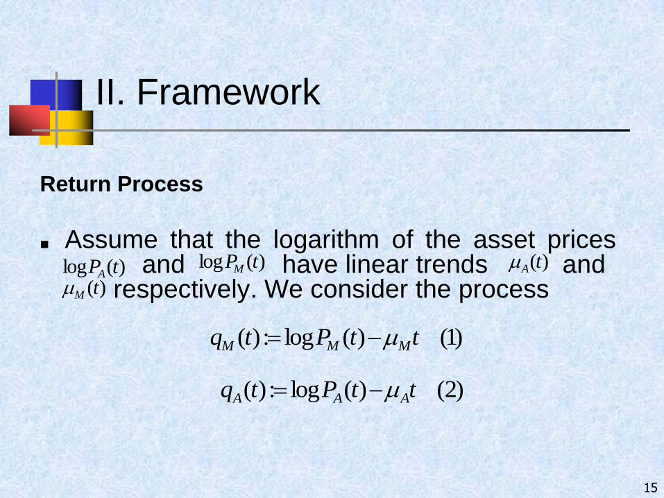
Return Process
■ Assume that the logarithm of the asset pricesand have linear trends and
respectively. We consider the process
15
)(log tPA)(log tPM )(tA
)(tM
)1()(log:)( ttPtq MMM
)2()(log:)( ttPtq AAA
II. Framework
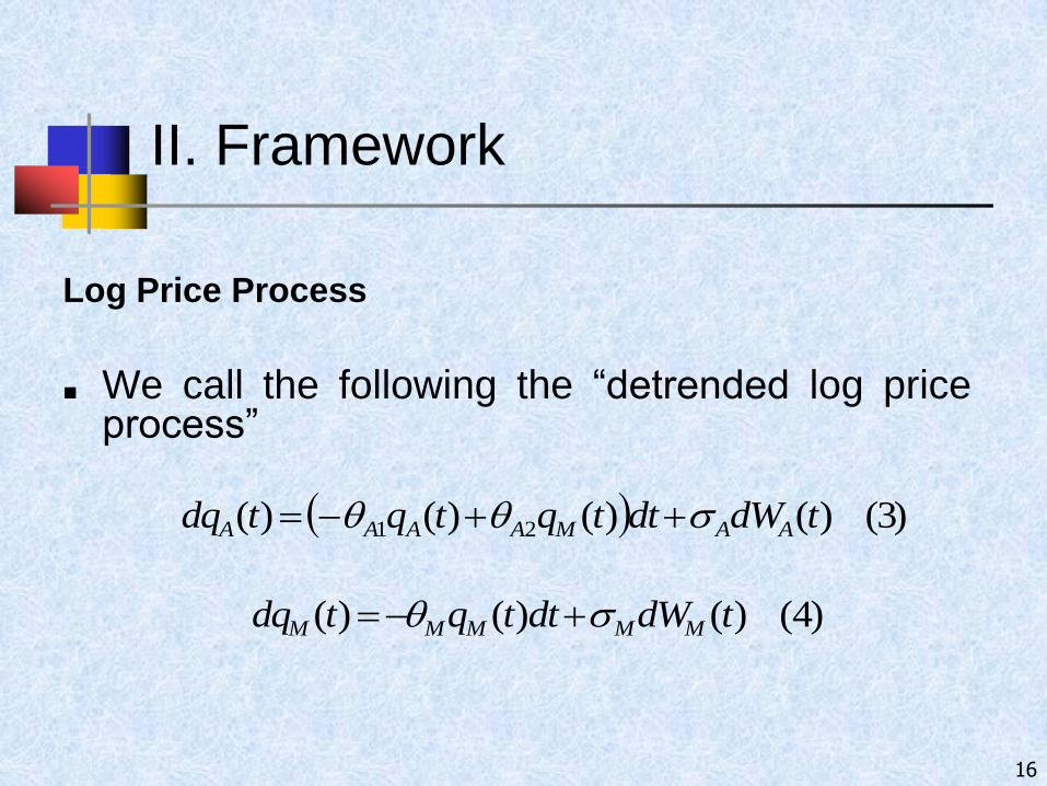
Log Price Process
■ We call the following the “detrended log priceprocess”
16
)3()()()()( 21 tdWdttqtqtdq AAMAAAA
)4()()()( tdWdttqtdq MMMMM
II. Framework
Log Price Process
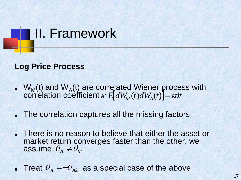
■ WM(t) and WA(t) are correlated Wiener process with correlation coefficient :
■ The correlation captures all the missing factors
■ There is no reason to believe that either the asset or market return converges faster than the other, we assume
■ Treat as a special case of the above17
dttdWtdWE AM )()(
MA 1
21 AA
II. Basic Framework
Proposition 1
■ The return vector,
can be written as:
18
)()(
),(
),(),( tQhtQ
thtr
thtrthtR
M
A
)5(
)(
0
)(
)1(0
)1()1()1(),(
)(
)()(
1
2)(
1
2
11
111
uHdW
e
eee
tQ
ee
eeeeeehthtR
ht
t ut
utut
MA
Aut
ht
htht
MA
Aht
M
A
M
AMA
MM
AAMMMA
III. CAPM Beta
■ Asset Return Covariance
conditional on time t, the covariance is linear in theinstantaneous covariance. Here refers to additivereturns from time t to time t + h
■ Market Return Autocovariance
19
,
MA
MA
h
M
MA
A
MA
h
M
h
rArMMA
AMAMM eeetrtrCov
1
2
1
2
1
2 11
2
1)(),(
11
22
2
1)(),( M
M
h
rMMMMM
M
ee
CovtrtrCov
)(trA
III. CAPM Beta
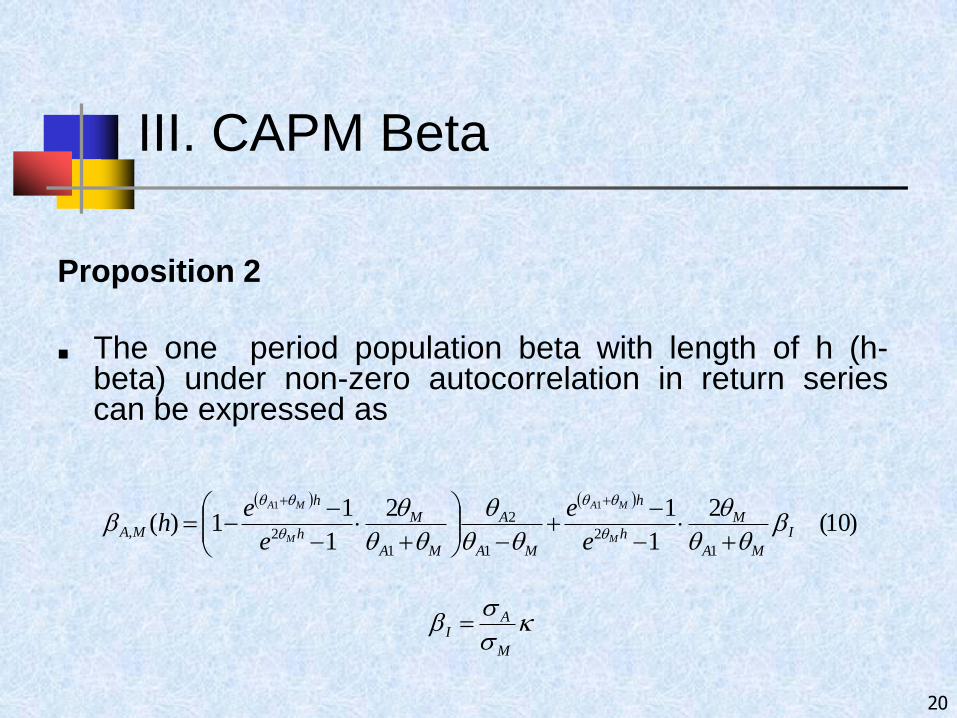
Proposition 2
■ The one period population beta with length of h (h-beta) under non-zero autocorrelation in return seriescan be expressed as
20
,
)10(2
1
12
1
11)(
1
2
1
2
1
2,
11
I
MA
Mh
h
MA
A
MA
Mh
h
MAM
MA
M
MA
e
e
e
eh
M
AI
III. CAPM Beta
CAPM h Beta
■ h-beta is a positive transformation of instantaneous beta
■ Instantaneous beta is considered to be underlying ortrue beta, but mainly because it’s a parameter of thetrue model
■ The strength of our approach is that we can assume thetrue beta to be the beta at any frequency and still carryout an analysis
21
I
III. CAPM Beta
CAPM h Beta
■ This gives an exact relationship between the h beta andthe instantaneous beta in terms of over andunderestimation for different h
■ All the parameters can be estimated, we shall discussthe results later
22
)11(2
)1(
)1(1)(
1
2
1
2,
1
I
MA
A
MA
Mh
h
IMAM
MA
e
eh
III. CAPM Beta
Monotonicity of Beta with respect to h
■ LL proves positive monotonicity under i.i.d multiplicativereturn assumptions, therefore, any test of the LL modelis an implicit test of monotonicity
■ With our bivariate log OU model, we can perform ananalysis of monotonicity on the measure of systematicrisk, the beta
23
III. CAPM Beta
Proposition 3
■ For the stationary case, with and the derivative
is monotonic with h
Comment: The monotonicity can be either increasing or decreasing, we give the relevant conditions
24
,
0M 01 A
h
h IMA
)(,
III. CAPM Beta
25
,
Figure I: Exact Beta vs. h
III. CAPM Beta
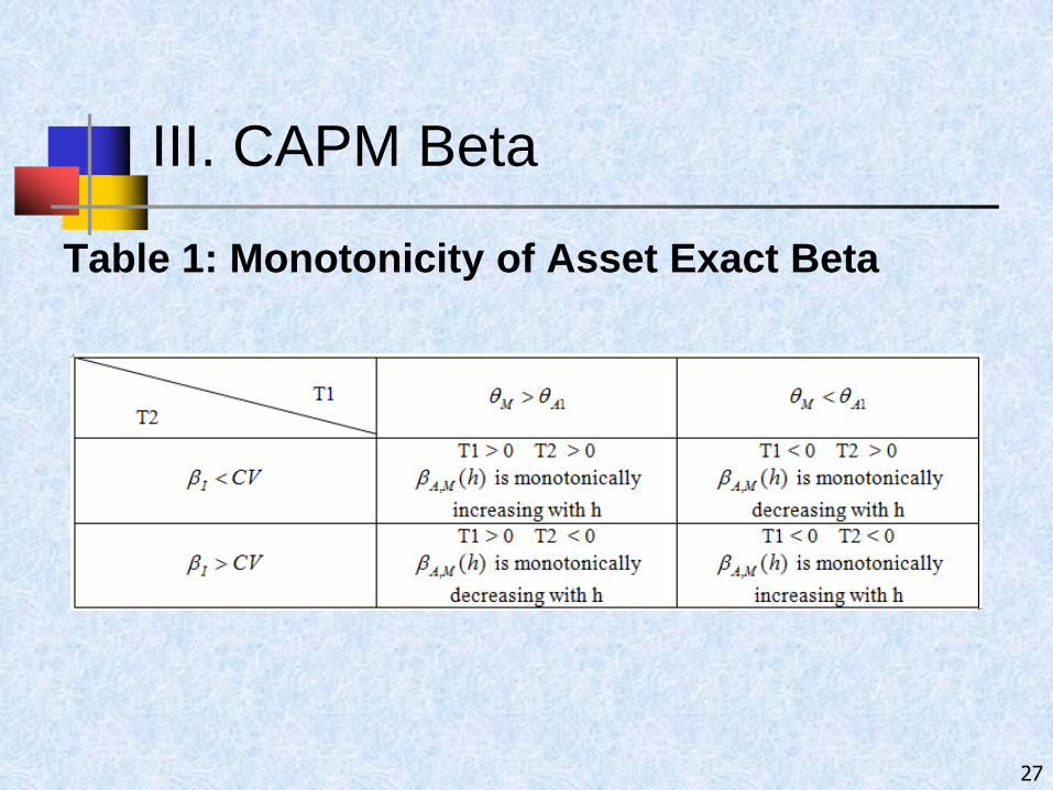
Monotonicity of Beta with respect to h
■ Whether the exact beta is monotonically increasing ordecreasing is governed by the signs of the first and thesecond term (T1 and T2 hereafter) of equation (11)
■ Equation (11) Revisited
26
,
)11(
(T2) (T1)
2
)1(
)1(1)(
1
2
1
2,
1
I
MA
A
MA
Mh
h
IMAM
MA
e
eh
III. CAPM Beta
27
,
Table 1: Monotonicity of Asset Exact Beta
III. CAPM Beta
Remark 1
■ If we let , it follows that
■ This shows that the instantaneous beta is the limitingvalue of beta. As the return interval decreases to zero,the value of beta converges to the instantaneous beta
28
,
0h
IMAh
h
)(lim ,0
III. CAPM Beta
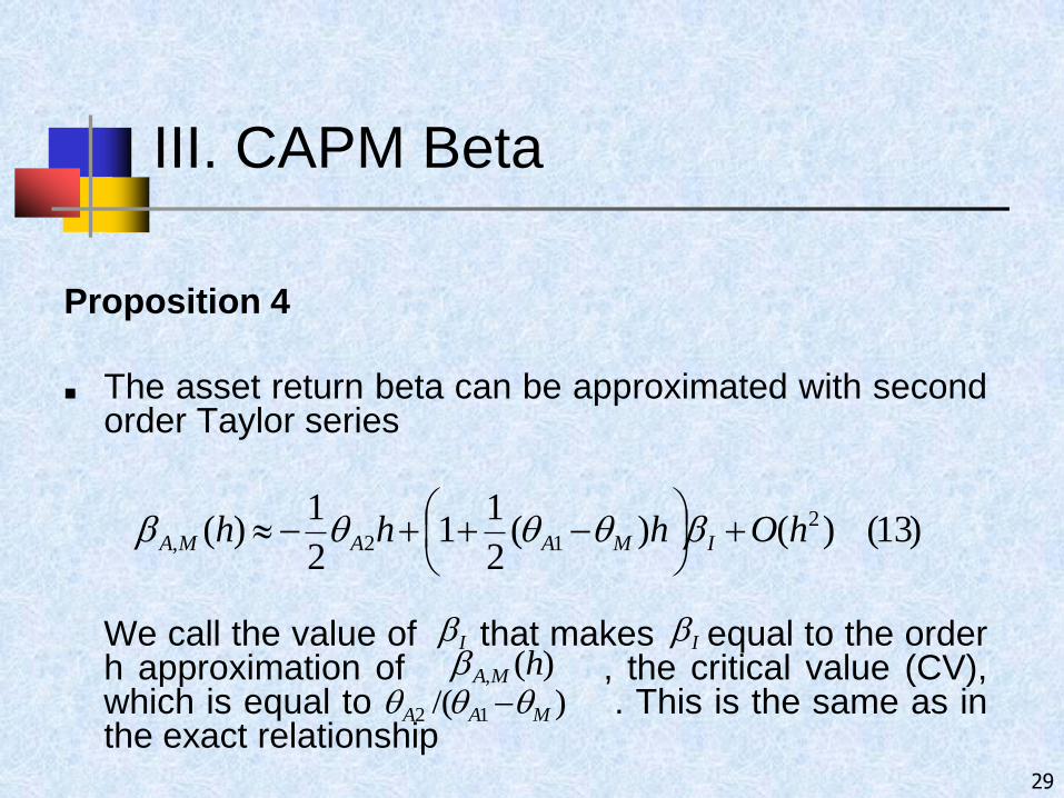
Proposition 4
■ The asset return beta can be approximated with secondorder Taylor series
We call the value of that makes equal to the orderh approximation of , the critical value (CV),which is equal to . This is the same as inthe exact relationship
29
,
)13()()(2
11
2
1)( 2
12, hOhhh IMAAMA
I I)(, hMA)/( 12 MAA
III. CAPM Beta
Proposition 4
■ It is an immediate consequence of Proposition 4 thatthe approximate sensitivity of the asset beta withrespect to the return measurement interval is
30
,
)14()(2
1
2
1)(12
,
IMAA
MA
h
h
III. CAPM Beta
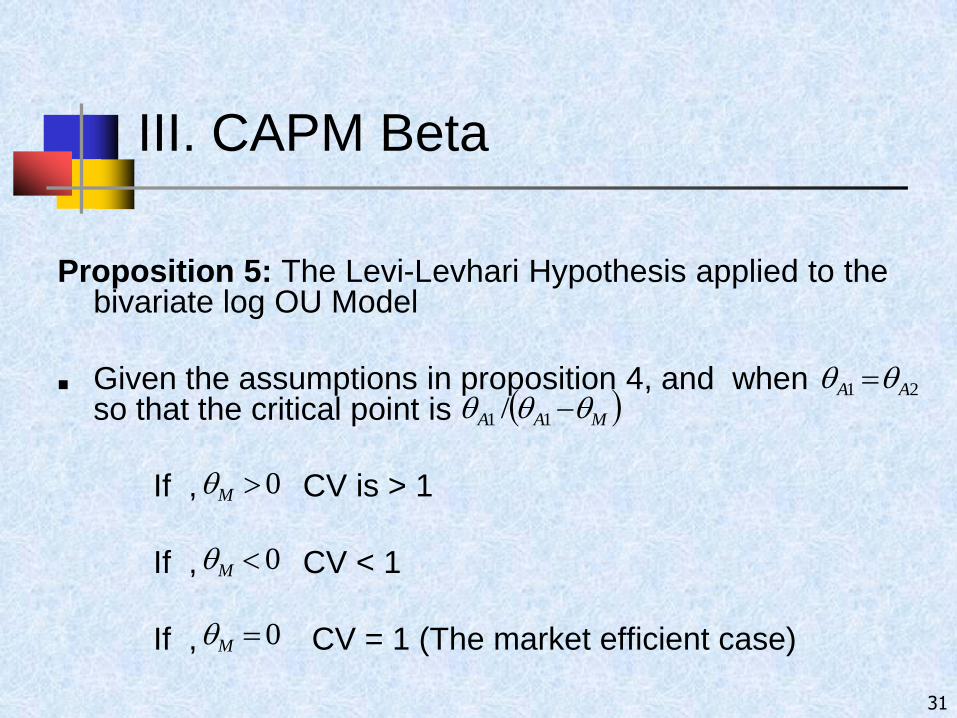
Proposition 5: The Levi-Levhari Hypothesis applied to thebivariate log OU Model
■ Given the assumptions in proposition 4, and when so that the critical point is
If , CV is > 1
If , CV < 1
If , CV = 1 (The market efficient case)
31
,
0M
0M
0M
21 AA MAA 11 /
III. CAPM Beta
Remark 2
■ The O(h) bias on caused by the intervallingeffect and the approximate sensitivity of the beta withrespect to h can be summarized as
If , : is upward biased and
If , : is downward biased and
If , : bias disappears and
32
,
)(, hMA
MA
AI
1
2IMA h )(, )(, hMA 0
)(,
h
hMA
MA
AI
1
2
MA
AI
1
2
IMA h )(,
IMA h )(,
)(, hMA
)(, hMA
0)(,
h
hMA
0)(,
h
hMA
III. CAPM Beta
Comments
■ Note that was assumed
■ The intervalling effect on the approximate beta and thespeed of the beta convergence to the instantaneous betadepends on the magnitude of , and
33
,
MA 1
1A M2A
III. CAPM Beta
■ The result shows that the intervalling effect can causethe beta to be over or underestimated depending on themagnitude of the true beta and the degree of auto-correlation
■ It is not in general true that under/over estimation isdetermined by whether the stock is aggressive ordefensive but it is determined by autocorrelation in thestock and the market returns
■ Our results show that both positive and negativemonotonicity can occur, this differs from LL
34
,
IV. Multiplicative Returns
Proposition 6: The LL Theorem for Multiplicative Returns for iid processes
■ Given the assumptions of Multiplicative Returns andwhen , and and the riskless rate are zero,
Case (i): the CAPM holds instantaneously, then
■ If and , we have
If ,
■ LL Result does not hold35
1A 2A M
)18()1)(exp(
)1))(exp())1(((5.)1)(exp((),,(
2
2222
h
hhhhMABeta
M
MIAIM
0M 1I 1),,( hMABeta
1I 1)))1(((5exp((.),,( 222 hhMABeta A
IV. Multiplicative Returns
Case (ii): the CAPM holds in multiplicative returns for all h, then
Then
■ In Case (ii), we have the Levhari-Levi Result
36
)20()1)(exp(
)1))(exp(5.exp()1((),,(
2
22
h
hhhhMABeta
M
MIMMII
)19(1))5.exp((
1))5.exp((2
2
h
h
MM
AAI
V. Some Empirical Findings
■ Sample Data: 50 randomly selected stocks fromS&P500 index from July 1, 2009 to July 1, 2010
■ Betas we wish to calculate are conditional but wenote that the formula do not depend upon initialvalues (See Equation (10) of Slide 20)
■ We estimate daily, weekly and monthly betas basedon one year of data, this is a snap shot one could dothis on a rolling basis. However it is the same datawe use for parameter estimation of the OU model
37
V. Some Empirical Findings
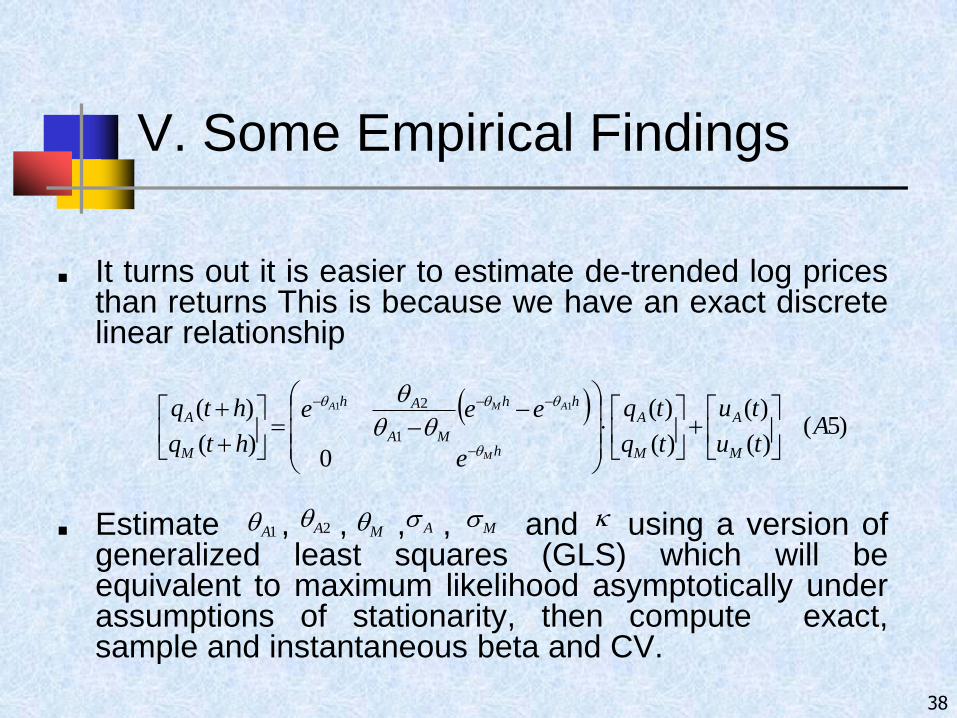
■ It turns out it is easier to estimate de-trended log pricesthan returns This is because we have an exact discretelinear relationship
■ Estimate , , , , and using a version ofgeneralized least squares (GLS) which will beequivalent to maximum likelihood asymptotically underassumptions of stationarity, then compute exact,sample and instantaneous beta and CV.
38
1A 2A M A M
)5(
)(
)(
)(
)(
0)(
)( 11
1
2
Atu
tu
tq
tq
e
eee
htq
htq
M
A
M
A
h
hh
MA
Ah
M
A
M
AMA
V. Some Empirical Findings
■ 24 out of 50 of the random sample of stocks have
■ All 50 of and were significantly different from 0 at5% confidence level while only 3 of were. 6 of
were significant at 10%
■ 20 of the beta plots are increasing and 30 of the plotsare decreasing
39
MA 1
M 1A
2A 2A
V. Some Empirical Findings
■ 16 of the empirical betas are monotonic, this might bethought of as a rejection of the theory. Howevermonotonic in population does not imply monotonic insample
■ In any case, we see this as a useful model rather than atrue description of the unknowable reality (We arepositivists!)
40
V. Some Empirical Findings
Table I: Number of Sample Stocks in Different Domain
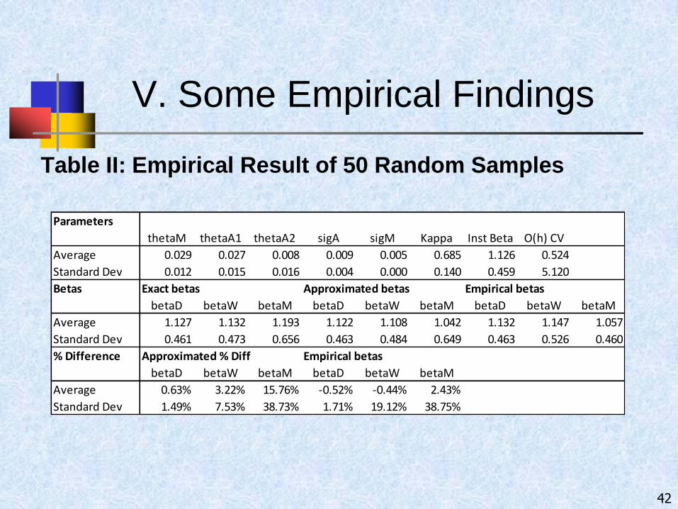
Average 1.127 1.132 1.193 1.122 1.108 1.042 1.132 1.147 1.057
Standard Dev 0.461 0.473 0.656 0.463 0.484 0.649 0.463 0.526 0.460
% Difference Approximated % Diff Empirical betas
betaD betaW betaM betaD betaW betaM
Average 0.63% 3.22% 15.76% -0.52% -0.44% 2.43%
Standard Dev 1.49% 7.53% 38.73% 1.71% 19.12% 38.75%
V. Some Empirical Findings
■ Percentage errors are calculated as (exact beta –alternative beta) / exact beta
■ Daily results are extremely good (The data does notknow that they are OU), weekly results are less goodand monthly results are unconvincing
■ The average of CV is less than the average of theinstantaneous beta and the average of exact betasare larger than that of the instantaneous beta for all h
■ We find that the average of daily beta < average ofweekly beta < average of monthly beta
43
V. Some Empirical Findings
Bekaert and Wang (2010)
44
V. Some Empirical Findings
Bekaert and Wang (2010)
45
VI. Conclusion
■ In this paper we have advocated the use of the OUmodel in modelling the intervalling effect to give usdeeper insight into the behavior of monotonicity, wedo not believe it is the true process governing allreturns. However over short horizons it seemsextremely good when compared with standardestimators
■ Allows us to generalise the LL hypothesis tosituations where both asset and market arecorrelated
■ It takes the discussion away from whether stocks areaggressive or defensive. Applicable to any one factormodel or to multi-factor models taking one factor at a
46
VI. Conclusion
■ The generalisation of the LL hypothesis is based onexact calculation. We can also approximate theresults using small – h asymptotics, we can easilydeal with both additive and multiplicative returns
■ We also show that beta will be monotonic in h
■ This creates a point which we call the critical valuebelow which beta is underestimated (against theinstantaneous beta) as h increases but the bias isdecreasing whilst above this point the beta isoverestimated as h increases
47
VI. Conclusion
Further work in this area is planned
■ Issues of overlapping data; building daily modelsbased on monthly or annual returns
■ Addressing issues of synchronicity with existingmodel, we can look at deterministic nonsynchronicitysuch as different market closing time for same asset
■ To deal with stochastic synchronicity, we would needto extend our model by randomizing the arrival timeof the data