Page 1
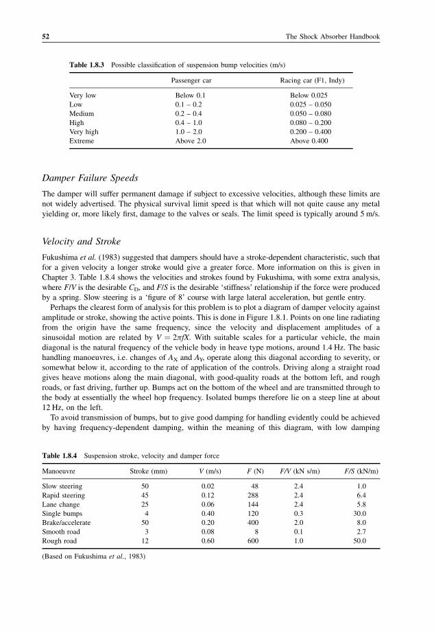
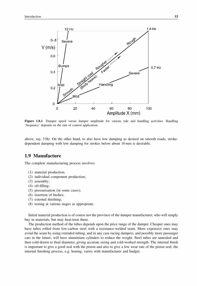
The Shock Absorber HandbookSecond Edition
John C. Dixon, Ph.D, F.I.Mech.E., F.R.Ae.S.Senior Lecturer in Engineering Mechanics
The Open University, Great Britain
This Work is a co-publication between Professional Engineering Publishing Ltd
and John Wiley and Sons, Ltd.
Page 3
The Shock Absorber HandbookSecond Edition
Page 4
Wiley-Professional Engineering Publishing Series
This series of books from John Wiley Ltd and Professional Engineering Publishing Ltd aims to
promote scientific and technical texts of exceptional academic quality that have a particular appeal to
the professional engineer.
Forthcoming titles:
Vehicle Particulate Emissions
Peter Eastwood
Suspension Analysis and Computational Geometry
John C. Dixon
Managing Reliability Growth in Engineering Design: Decisions, Data and Modelling
Lesley Walls and John Quigley
Page 5
The Shock Absorber HandbookSecond Edition
John C. Dixon, Ph.D, F.I.Mech.E., F.R.Ae.S.Senior Lecturer in Engineering Mechanics
The Open University, Great Britain
This Work is a co-publication between Professional Engineering Publishing Ltd
and John Wiley and Sons, Ltd.
Page 6
This Work is a co-publication between Professional Engineering Publishing Ltd and John Wiley and Sons, Ltd.
Previously published as The Shock Absorber Handbook, 1st Edition, by The Society of Automotive Engineers, Inc,
1999, ISBN 0-7680-0050-5.
By the same author: Tires, Suspension and Handling (SAE).
Copyright � 2007 John Wiley & Sons Ltd, The Atrium, Southern Gate, Chichester,
West Sussex PO19 8SQ, England
Telephone (þ44) 1243 779777
Email (for orders and customer service enquiries): [email protected]
Visit our Home Page on www.wiley.com
All Rights Reserved. No part of this publication may be reproduced, stored in a retrieval system or transmitted in
any form or by any means, electronic, mechanical, photocopying, recording, scanning or otherwise, except under
the terms of the Copyright, Designs and Patents Act 1988 or under the terms of a licence issued by the Copyright
Licensing Agency Ltd, 90 Tottenham Court Road, London W1T 4LP, UK, without the permission in writing of the
Publisher. Requests to the Publisher should be addressed to the Permissions Department, John Wiley & Sons Ltd,
The Atrium, Southern Gate, Chichester, West Sussex PO19 8SQ, England, or emailed to [email protected] ,
or faxed to (þ44) 1243 770620.
Designations used by companies to distinguish their products are often claimed as trademarks. All brand names
and product names used in this book are trade names, service marks, trademarks or registered trademarks of their
respective owners. The Publisher is not associated with any product or vendor mentioned in this book.
This publication is designed to provide accurate and authoritative information in regard to the subject matter
covered. It is sold on the understanding that the Publisher is not engaged in rendering professional services.
If professional advice or other expert assistance is required, the services of a competent professional should be sought.
Anniversary Logo Design: Richard J. Pacifico
British Library Cataloguing in Publication Data
A catalogue record for this book is available from the British Library
ISBN 978-0-470-51020-9 (HB)
Typeset in 10/12 pt Times by Thomson Digital, India
Printed and bound in Great Britain by Antony Rowe Ltd, Chippenham, Wiltshire
This book is printed on acid-free paper responsibly manufactured from sustainable forestry
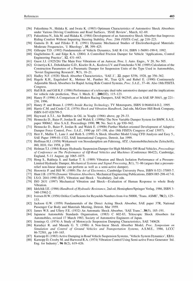
in which at least two trees are planted for each one used for paper production.
Page 7
Disclaimer: This book is not intended as a guide for vehicle modification, and anyone who
uses it as such does so entirely at their own risk. Testing vehicle performance may be
dangerous. The author and publisher are not liable for consequential damage arising from
application of any information in this book.
Page 9
Contents
Preface xiii
Acknowledgements xv
1 Introduction 1
1.1 History 1
1.2 Types of Friction 15
1.3 Damper Configurations 17
1.4 Ride-Levelling Dampers 33
1.5 Position-Dependent Dampers 35
1.6 General Form of the Telescopic Damper 37
1.7 Mountings 42
1.8 Operating Speeds and Strokes 47
1.9 Manufacture 53
1.10 Literature Review 54
2 Vibration Theory 61
2.1 Introduction 61
2.2 Free Vibration Undamped (1-dof) 61
2.3 Free Vibration Damped (1-dof) 63
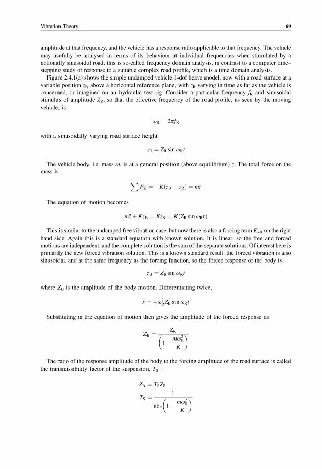
2.4 Forced Vibration Undamped (1-dof) 68
2.5 Forced Vibration Damped (1-dof) 71
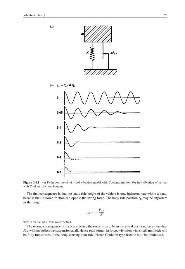
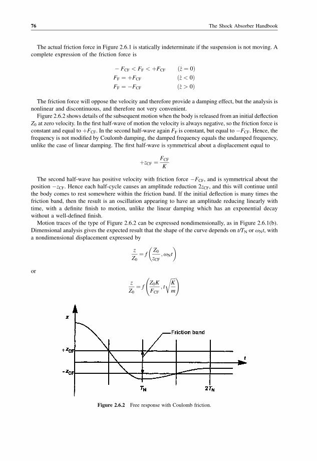
2.6 Coulomb Damping 74
2.7 Quadratic Damping 77
2.8 Series Stiffness 79
2.9 Free Vibration Undamped (2-dof) 85
2.10 Free Vibration Damped (2-dof) 85
2.11 The Resonant Absorber 86
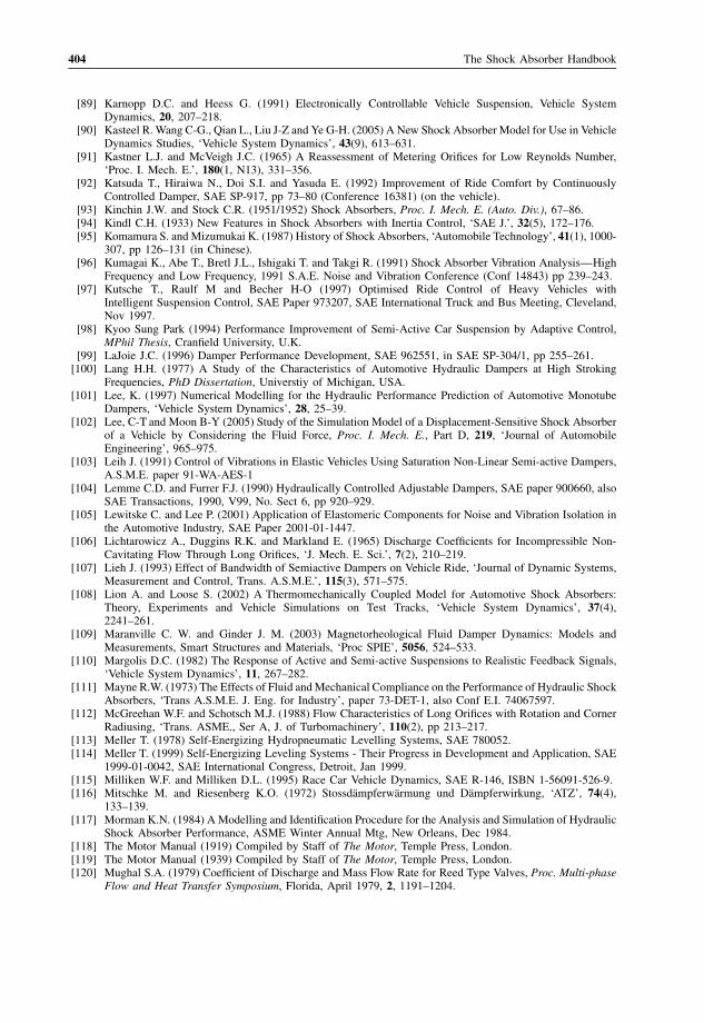
2.12 Damper Models in Ride and Handling 87
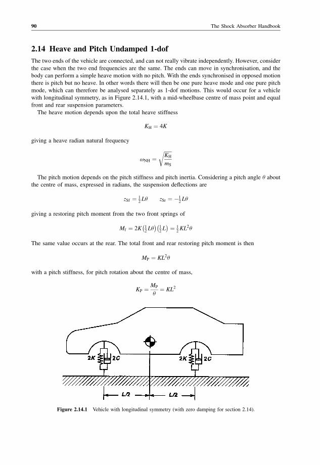
2.13 End Frequencies 88
2.14 Heave and Pitch Undamped 1-dof 90
2.15 Heave and Pitch Damped 1-dof 91
2.16 Roll Vibration Undamped 93
Page 10
2.17 Roll Vibration Damped 94
2.18 Heave-and-Pitch Undamped 2-dof 95
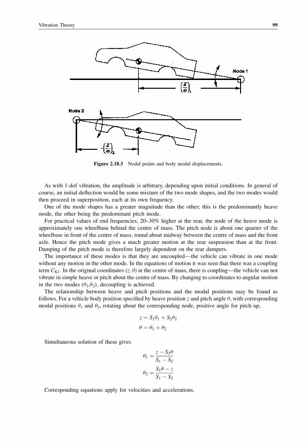
2.19 Heave-and-Pitch Damped 2-dof Simplified 100
2.20 Heave-and-Pitch Damped 2-dof Full Analysis 102
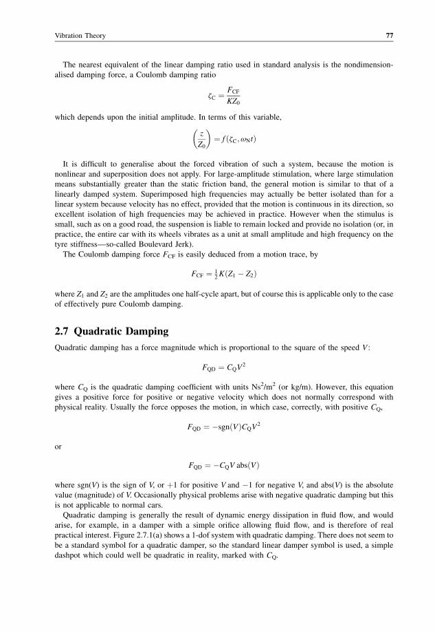
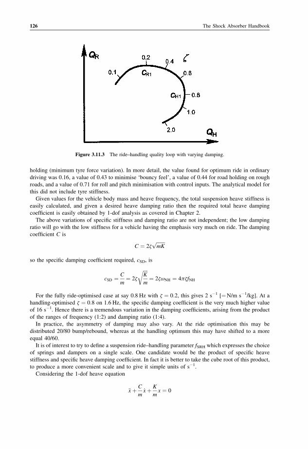
3 Ride and Handling 105
3.1 Introduction 105
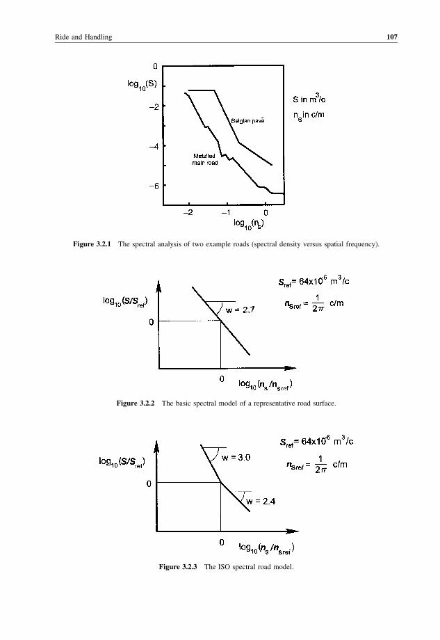
3.2 Modelling the Road 105
3.3 Ride 111
3.4 Time-Domain Ride Analysis 113
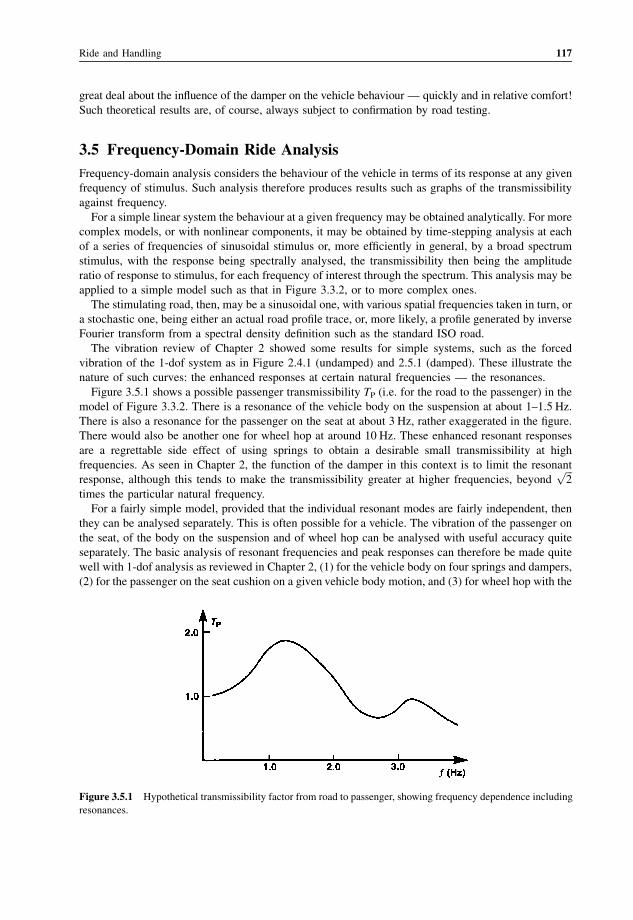
3.5 Frequency-Domain Ride Analysis 117
3.6 Passenger on Seat 118
3.7 Wheel Hop 119
3.8 Handling 120
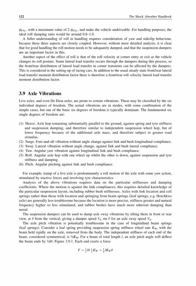
3.9 Axle Vibrations 122
3.10 Steering Vibrations 124
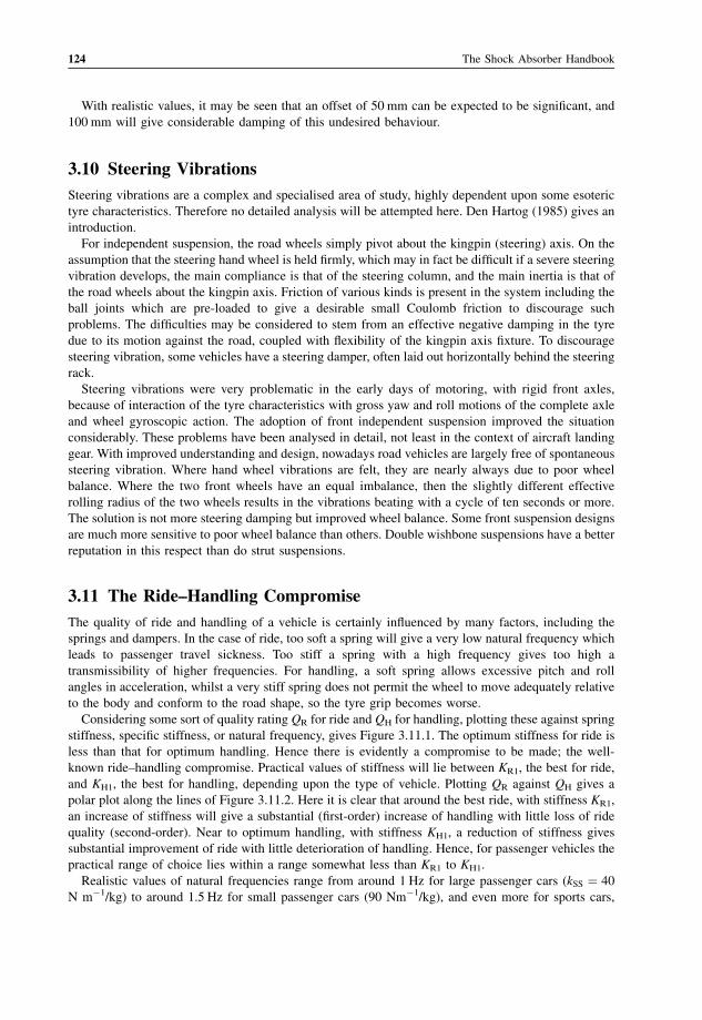
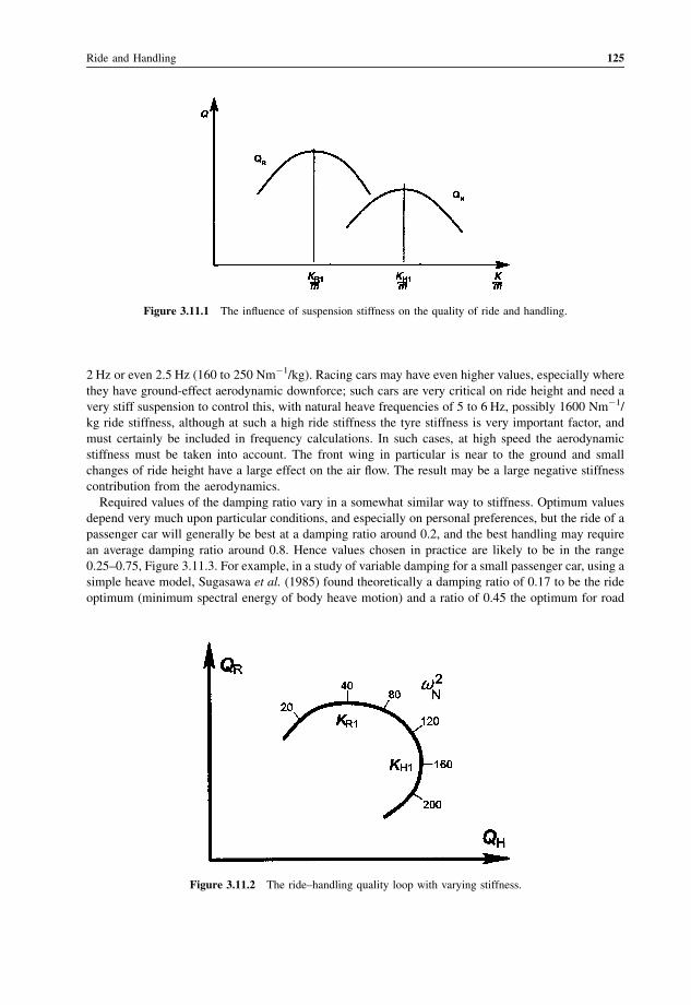
3.11 The Ride–Handling Compromise 124
3.12 Damper Optimisation 129
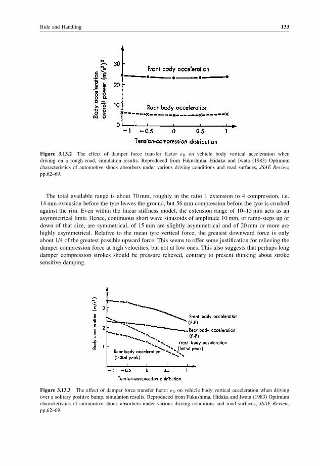
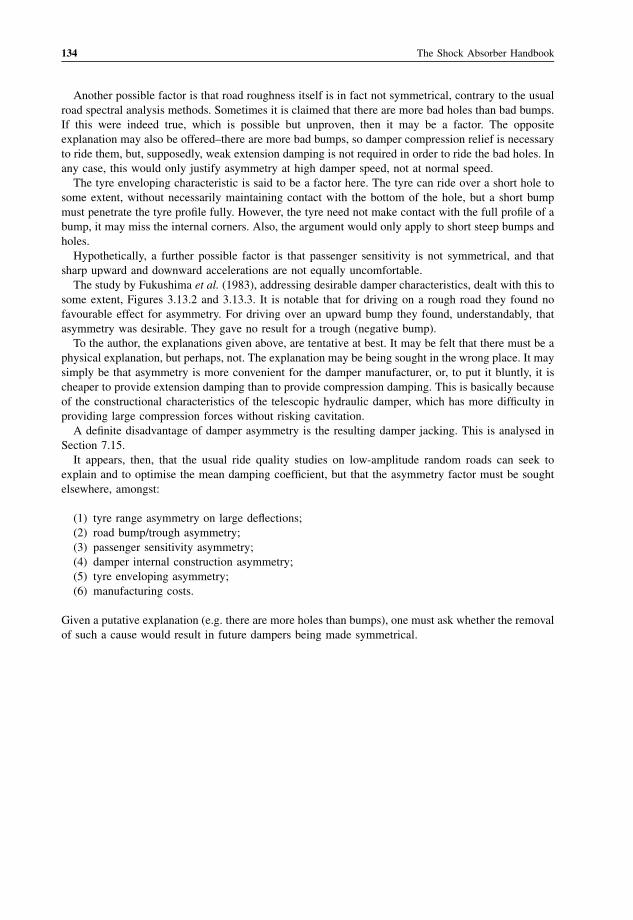
3.13 Damper Asymmetry 131
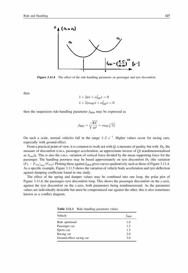
4 Installation 135
4.1 Introduction 135
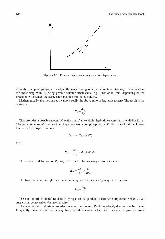
4.2 Motion Ratio 135
4.3 Displacement Method 137
4.4 Velocity Diagrams 138
4.5 Computer Evaluation 138
4.6 Mechanical Displacement 138
4.7 Effect of Motion Ratio 139
4.8 Evaluation of Motion Ratio 142
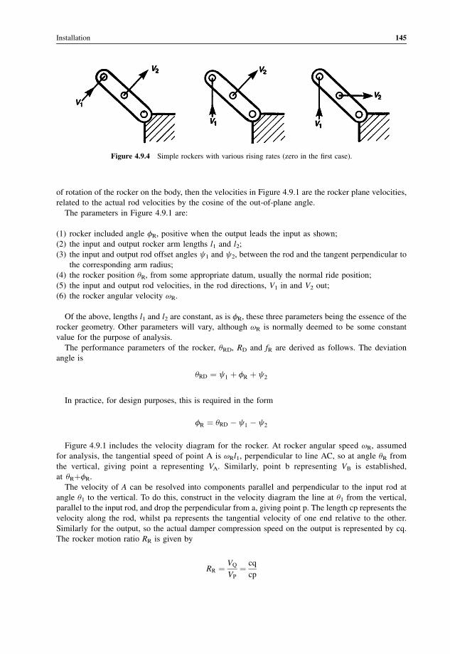
4.9 The Rocker 142
4.10 The Rigid Arm 148
4.11 Double Wishbones 150
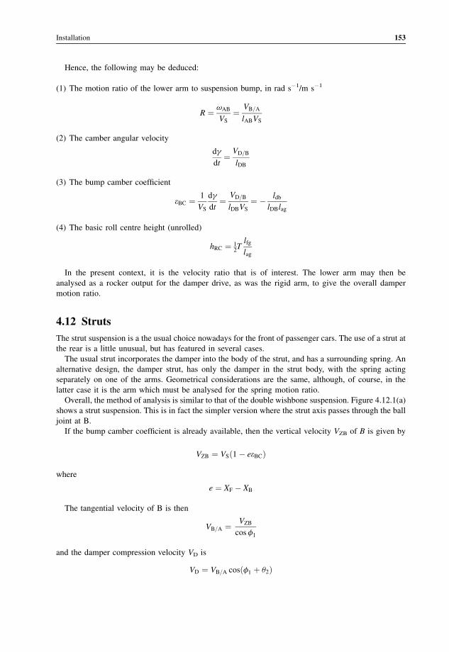
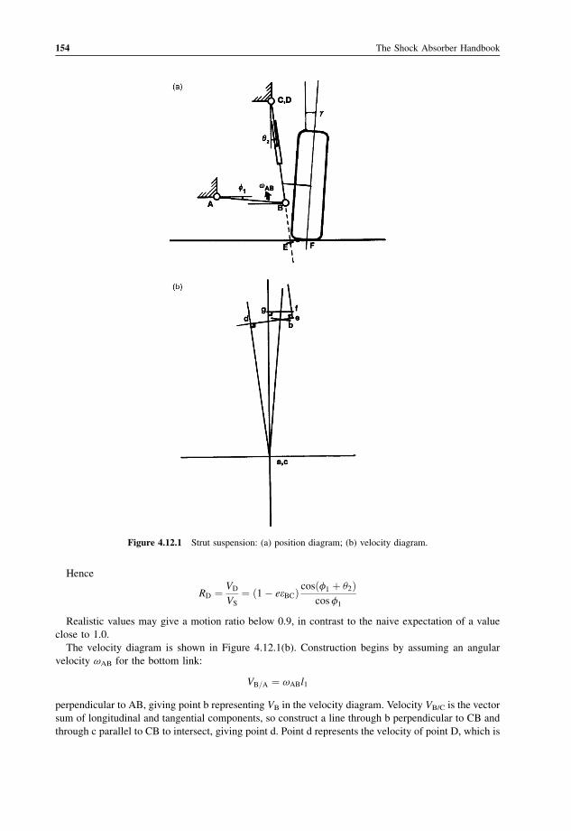
4.12 Struts 153
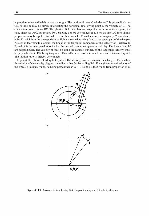
4.13 Pushrods and Pullrods 155
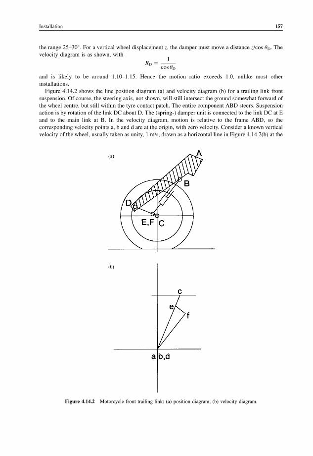
4.14 Motorcycle Front Suspensions 156
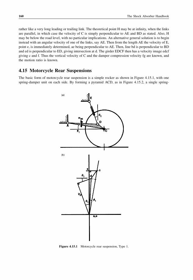
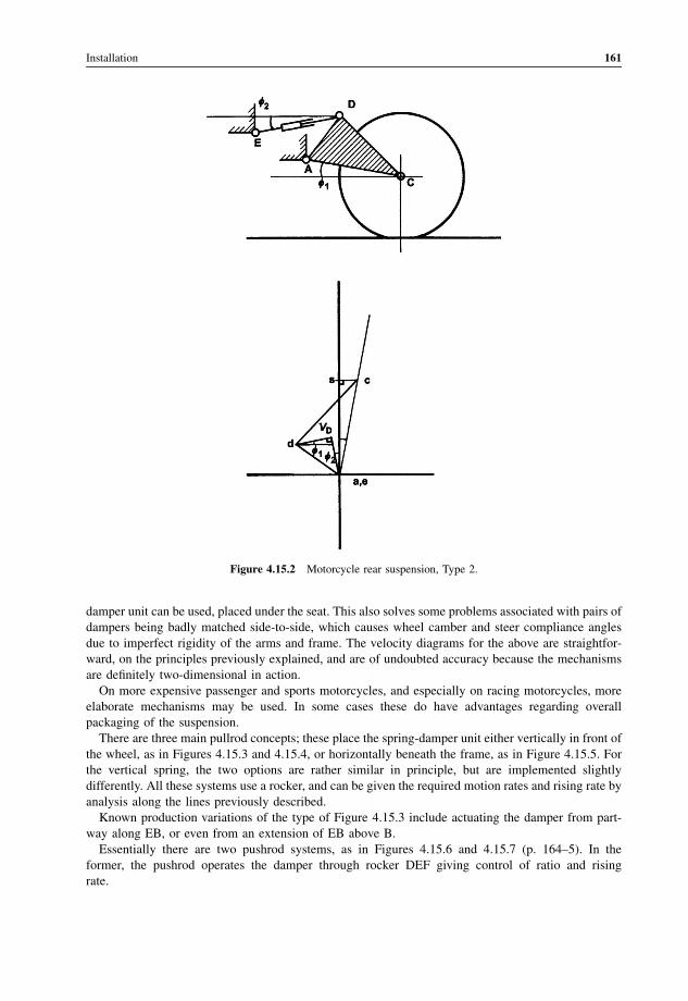
4.15 Motorcycle Rear Suspensions 160
4.16 Solid Axles 165
4.17 Dry Scissor Dampers 168
5 Fluid Mechanics 169
5.1 Introduction 169
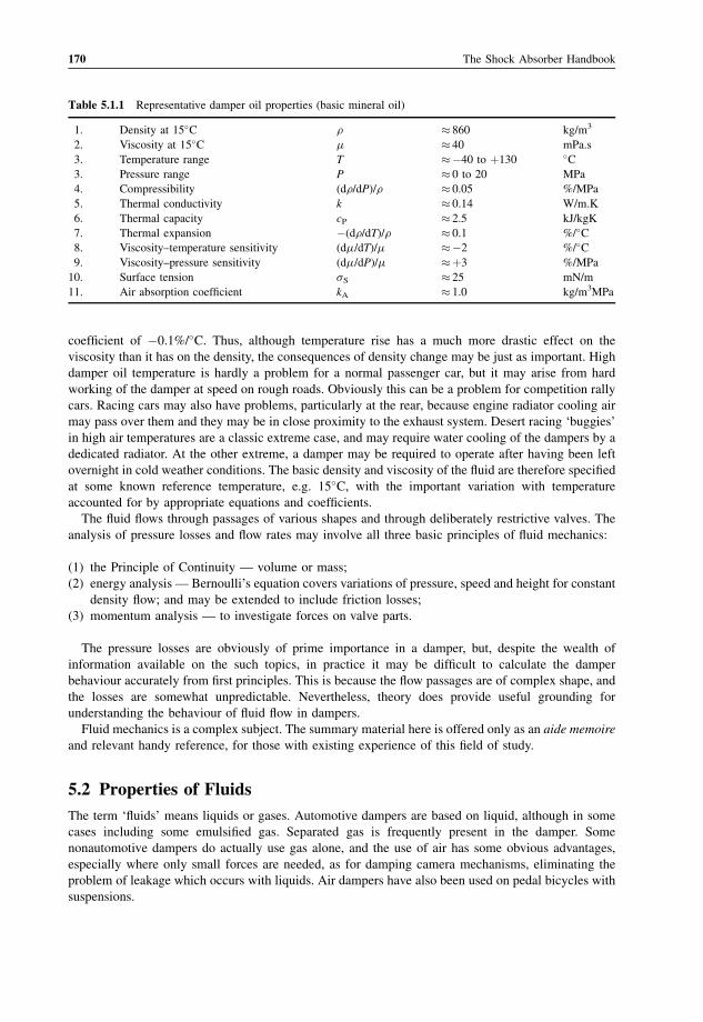
5.2 Properties of Fluids 170
5.3 Chemical Properties 171
5.4 Density 171
5.5 Thermal Expansion 172
viii Contents
Page 11
5.6 Compressibility 172
5.7 Viscosity 173
5.8 Thermal Capacity 175
5.9 Thermal Conductivity 176
5.10 Vapour Pressure 176
5.11 Gas Density 176
5.12 Gas Viscosity 177
5.13 Gas Compressibility 177
5.14 Gas Absorbability 177
5.15 Emulsification 179
5.16 Continuity 188
5.17 Bernoulli’s Equation 188
5.18 Fluid Momentum 189
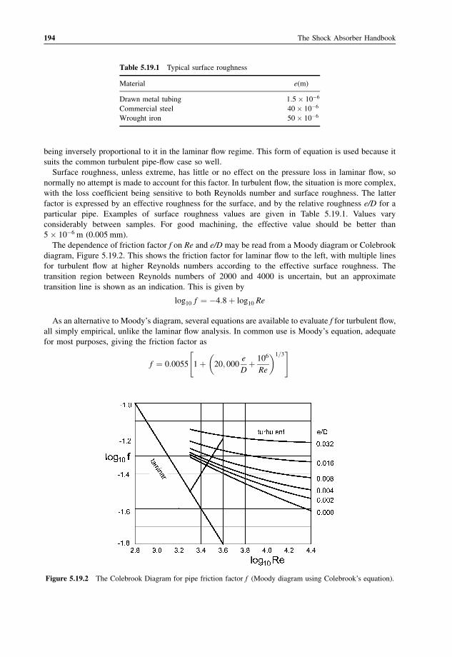
5.19 Pipe Flow 191
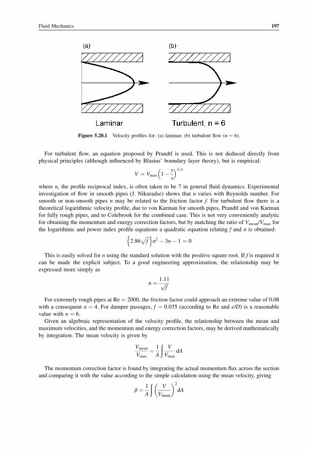
5.20 Velocity Profiles 196
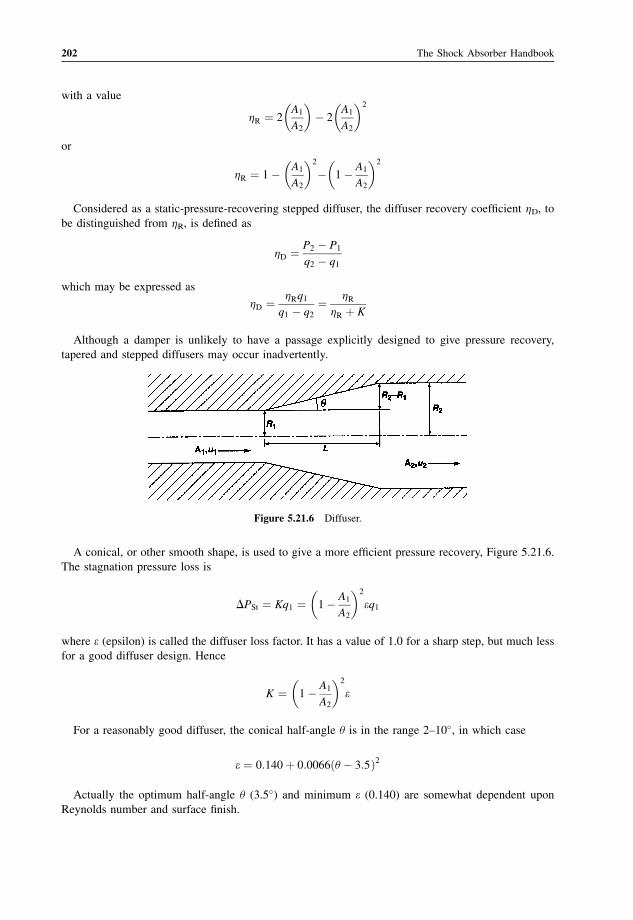
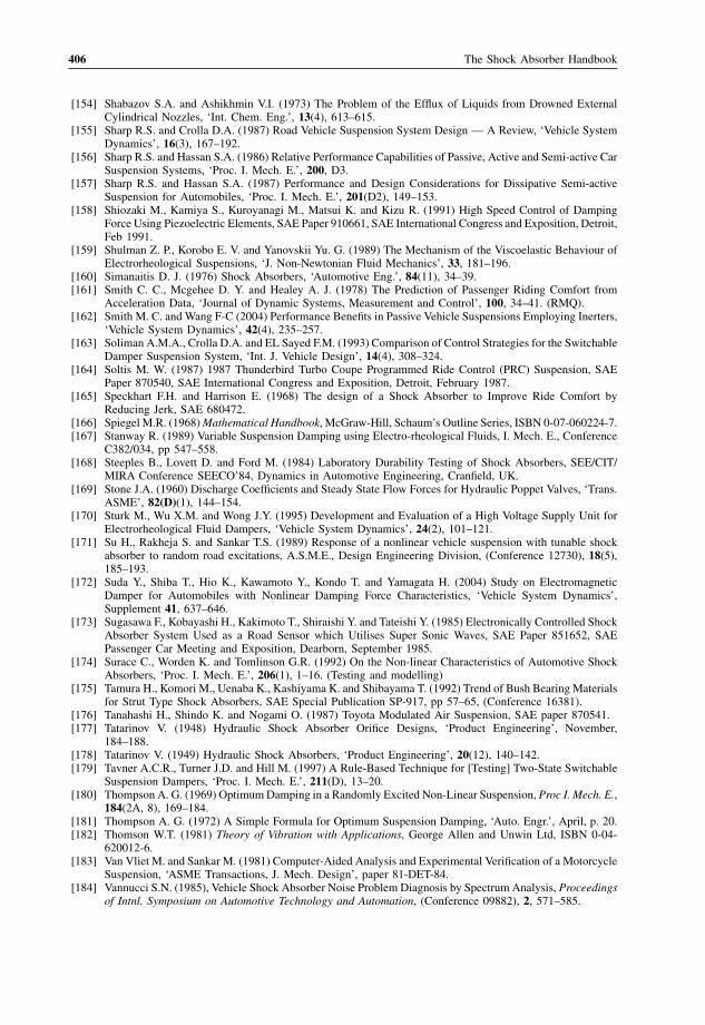
5.21 Other Losses 199
5.22 The Orifice 203
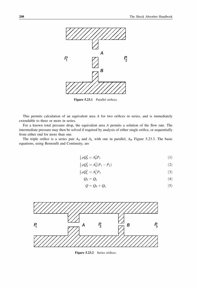
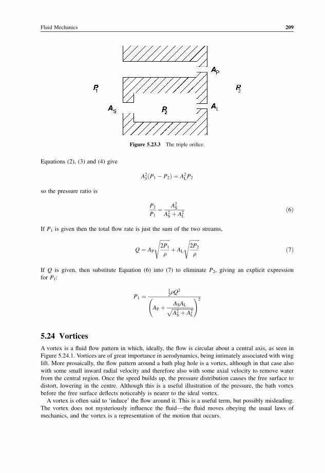
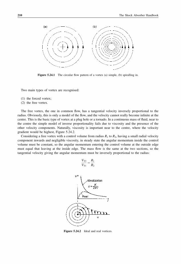
5.23 Combined Orifices 207
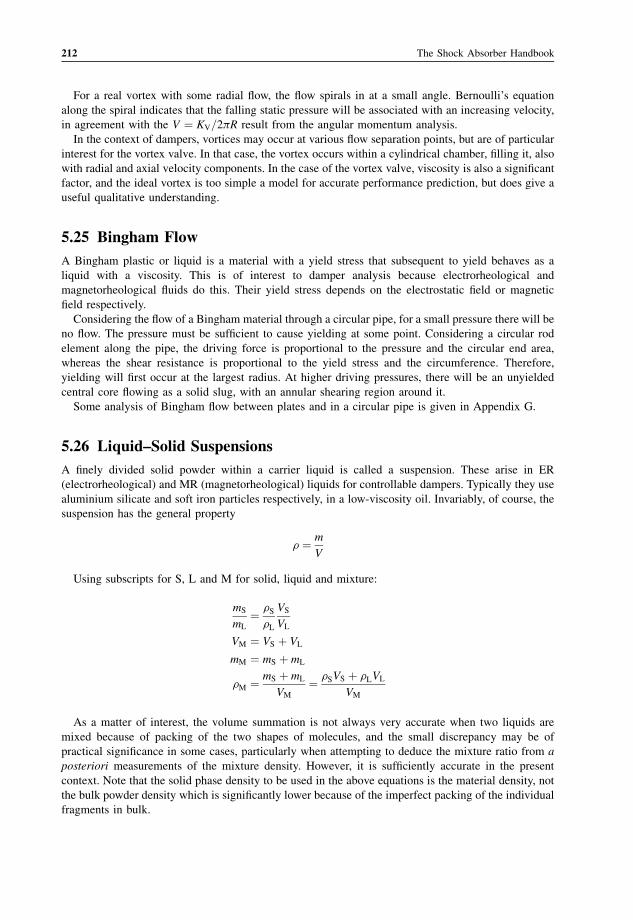
5.24 Vortices 209
5.25 Bingham Flow 212
5.26 Liquid–Solid Suspensions 212
5.27 ER and MR Fluids 214
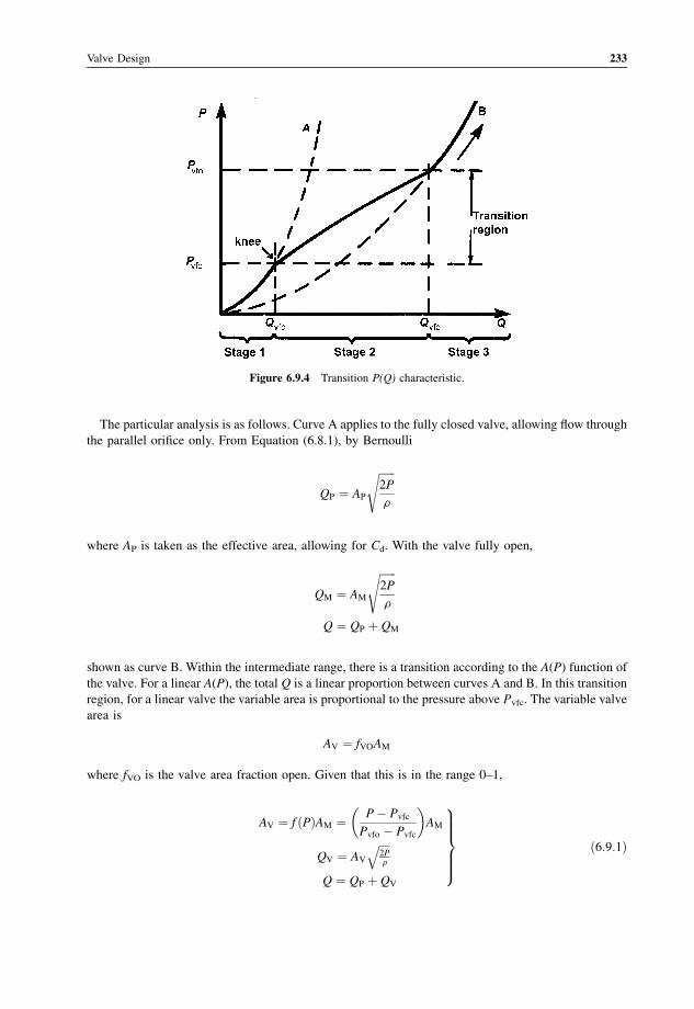
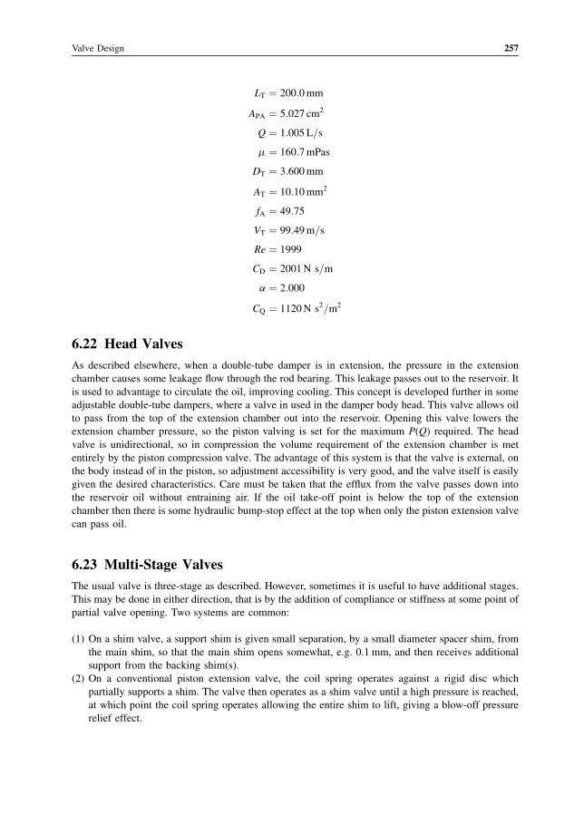
6 Valve Design 2176.1 Introduction 217
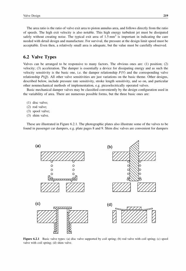
6.2 Valve Types 219
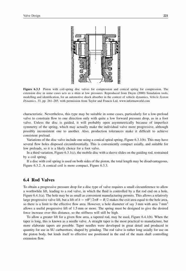
6.3 Disc Valves 220
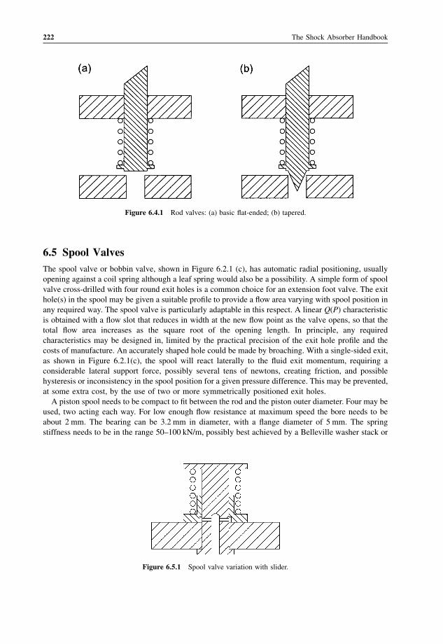
6.4 Rod Valves 221
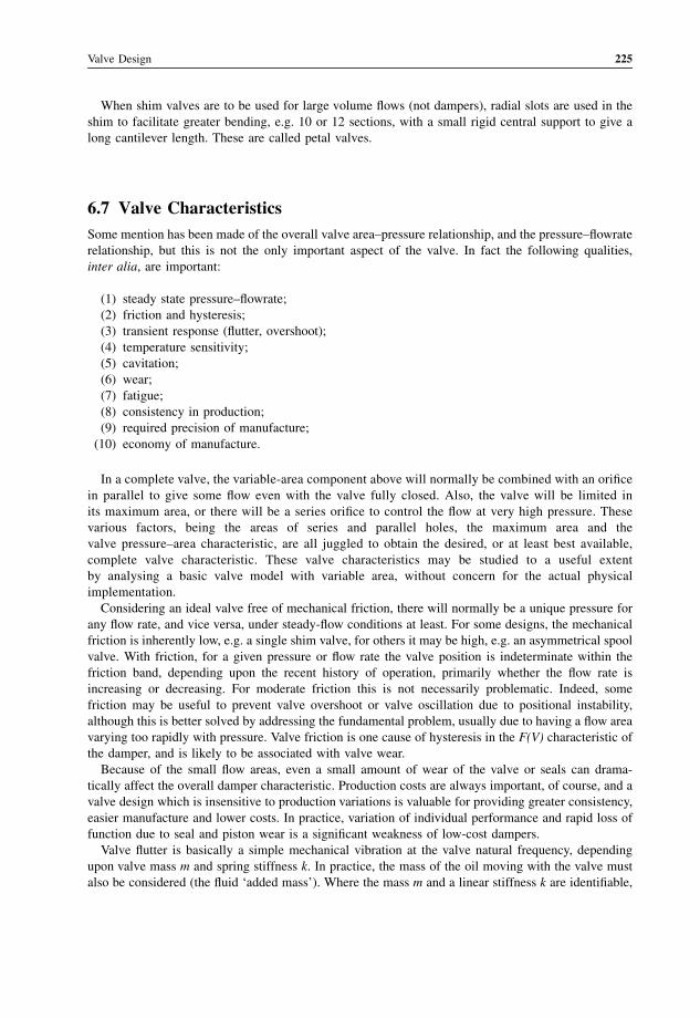
6.5 Spool Valves 222
6.6 Shim Valves 223
6.7 Valve Characteristics 225
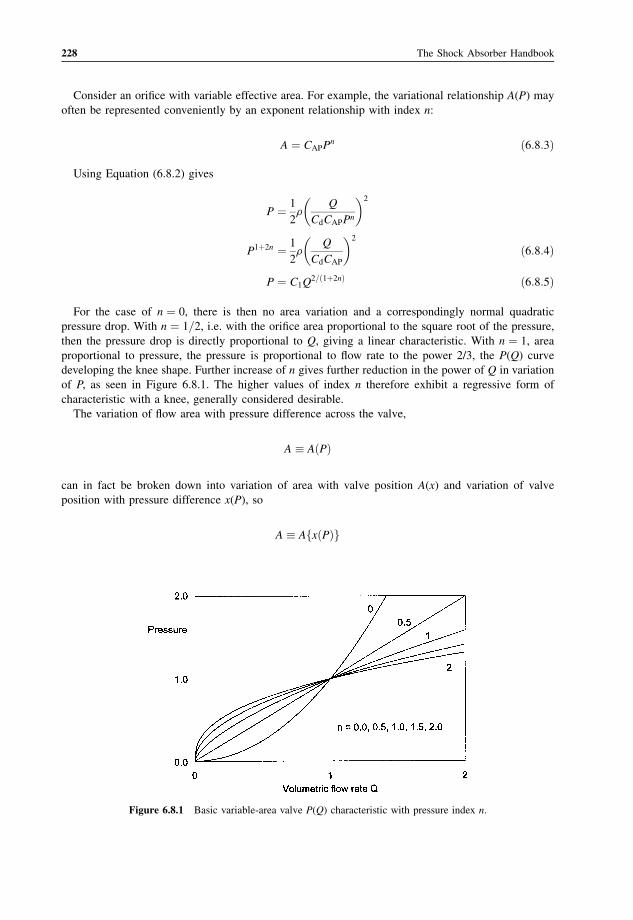
6.8 Basic Valve Models 227
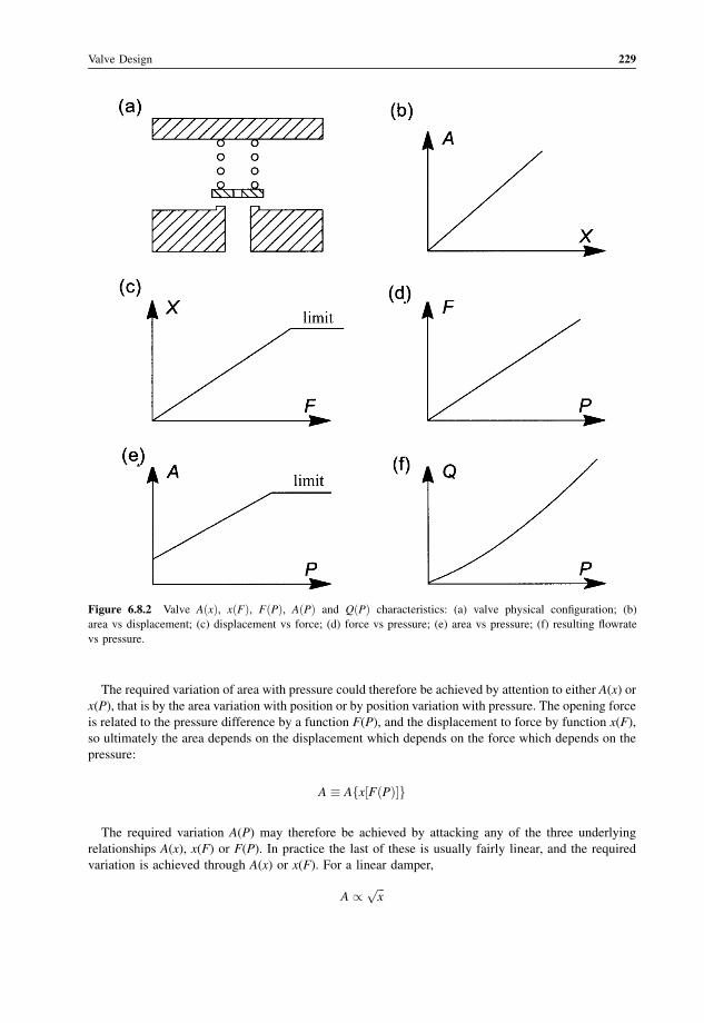
6.9 Complete Valve Models 230
6.10 Solution of Valve Flow 235
6.11 Temperature Compensation 237
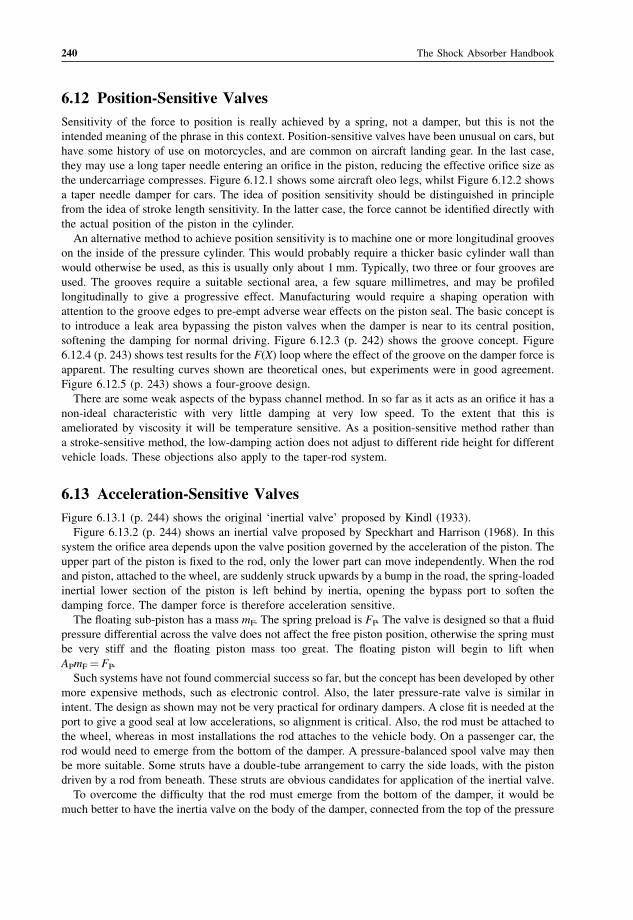
6.12 Position-Sensitive Valves 240
6.13 Acceleration-Sensitive Valves 240
6.14 Pressure-Rate Valves 243
6.15 Frequency-Sensitive Valves 245
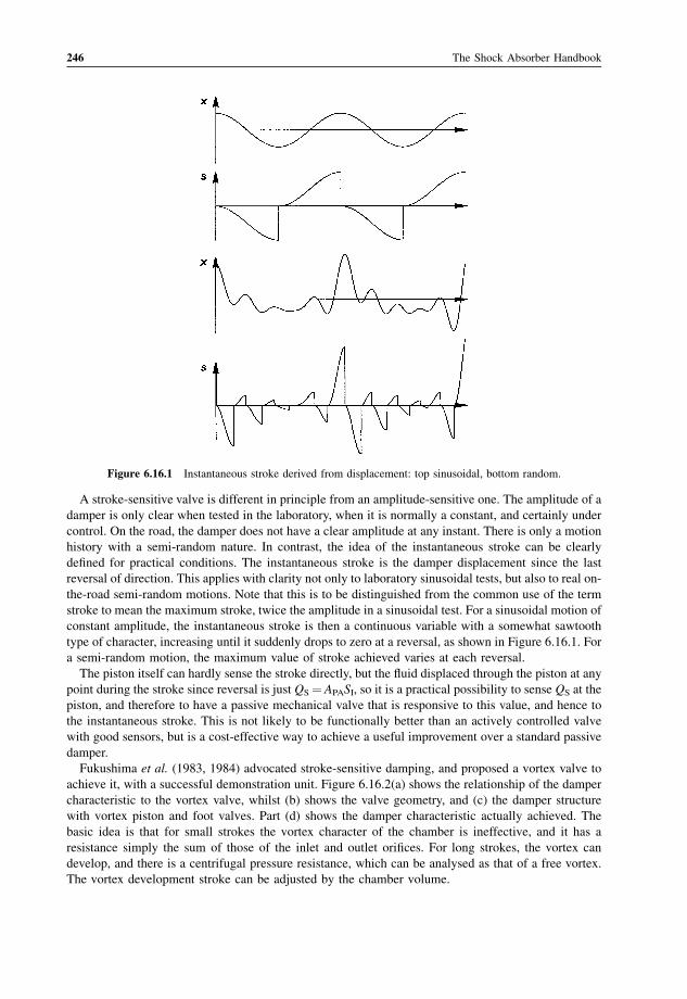
6.16 Stroke-Sensitive Valves 245
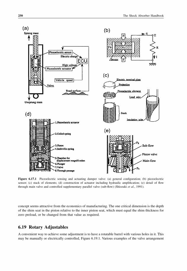
6.17 Piezoelectric Valves 249
6.18 Double-Acting Shim Valves 249
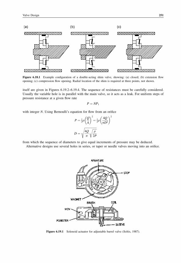
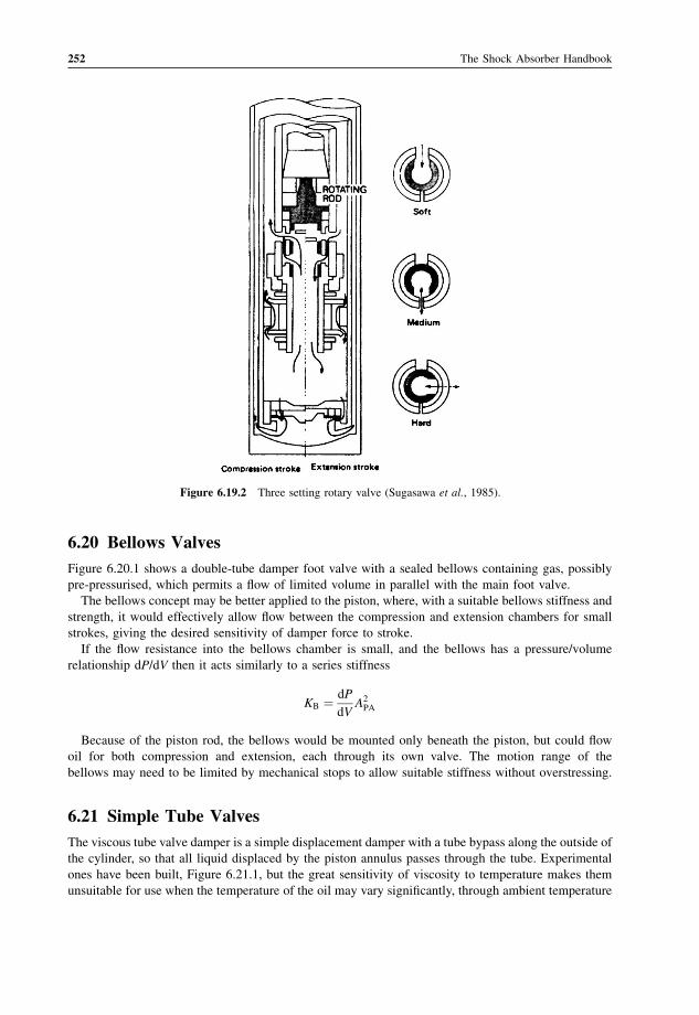
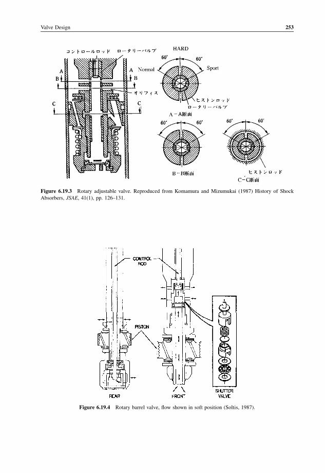
6.19 Rotary Adjustables 250
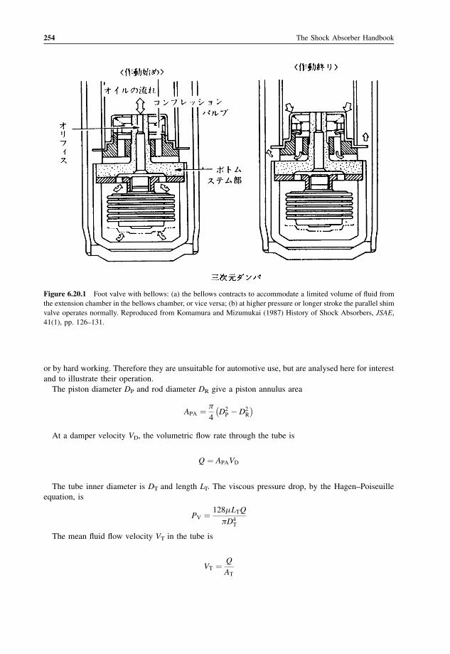
6.20 Bellows Valves 252
6.21 Simple Tube Valves 252
Contents ix
Page 12
6.22 Head Valves 257
6.23 Multi-Stage Valves 257
7 Damper Characteristics 259
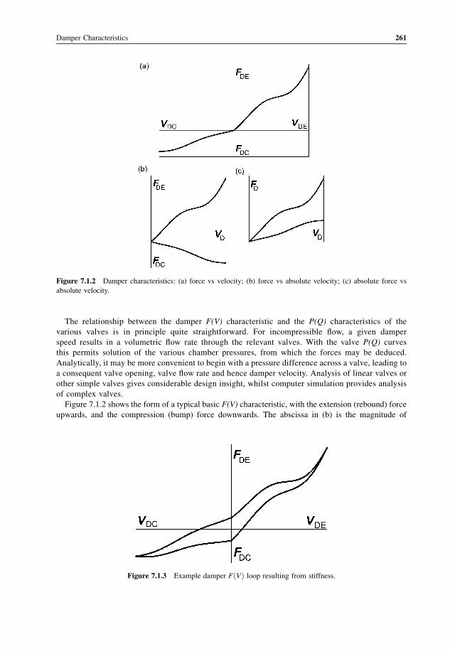
7.1 Introduction 259
7.2 Basic Damper Parameters 263
7.3 Mechanical Friction 265
7.4 Static Forces 268
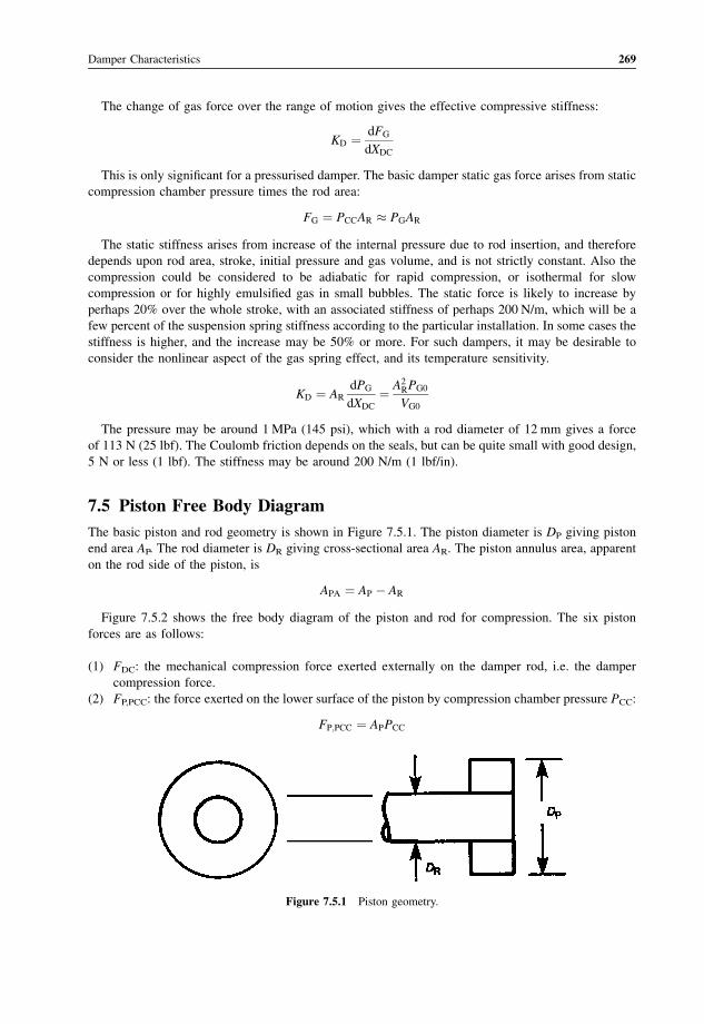
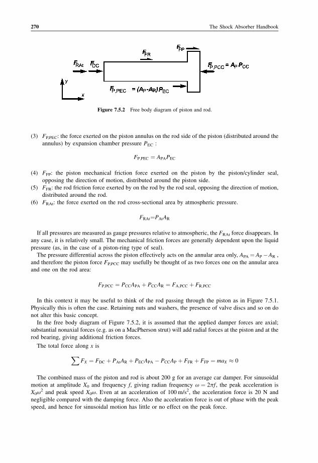
7.5 Piston Free Body Diagram 269
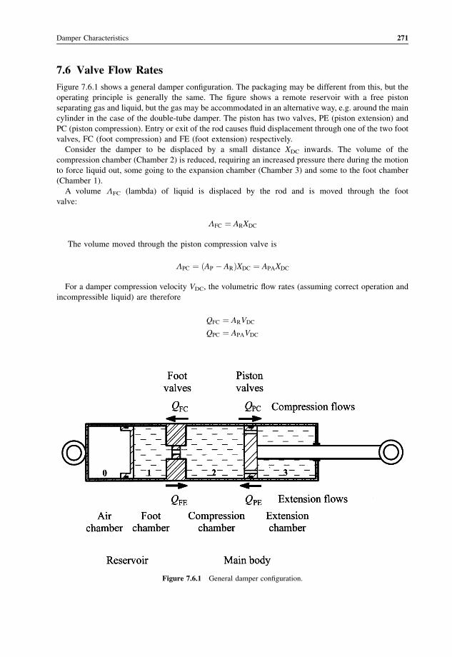
7.6 Valve Flow Rates 271
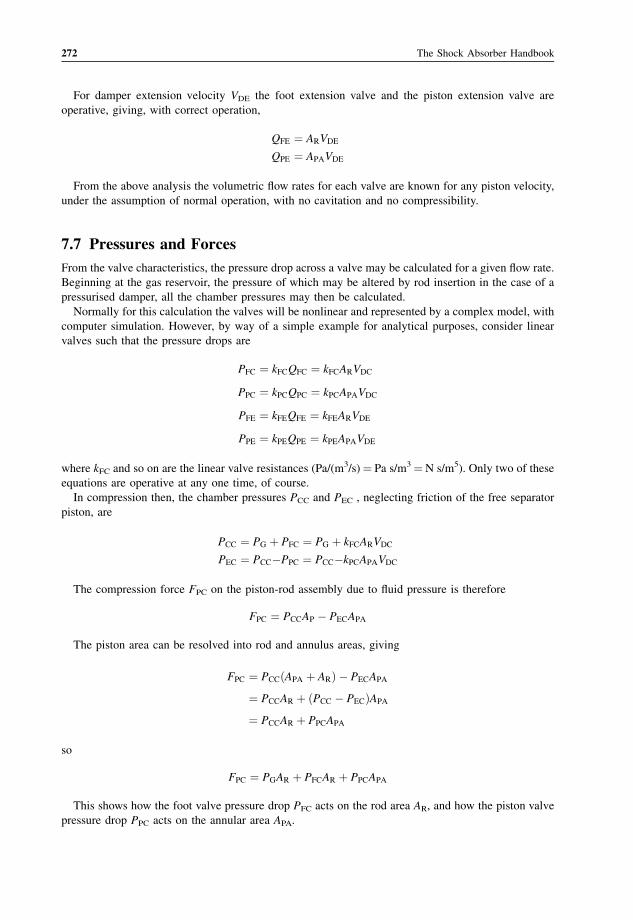
7.7 Pressures and Forces 272
7.8 Linear Valve Analysis 273
7.9 Cavitation 274
7.10 Temperature 276
7.11 Compressibility 276
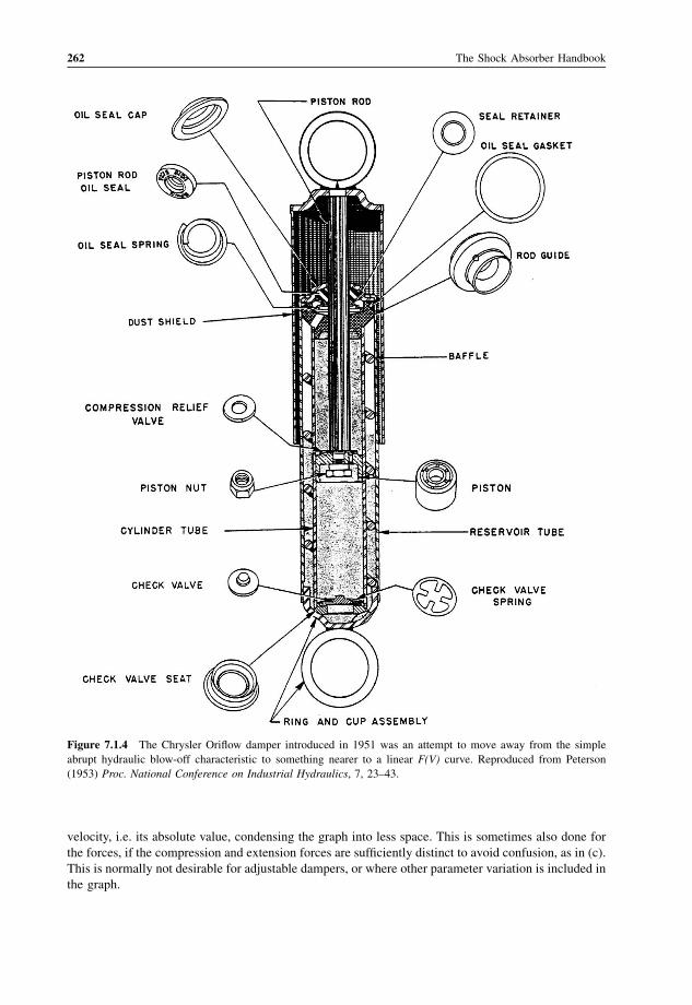
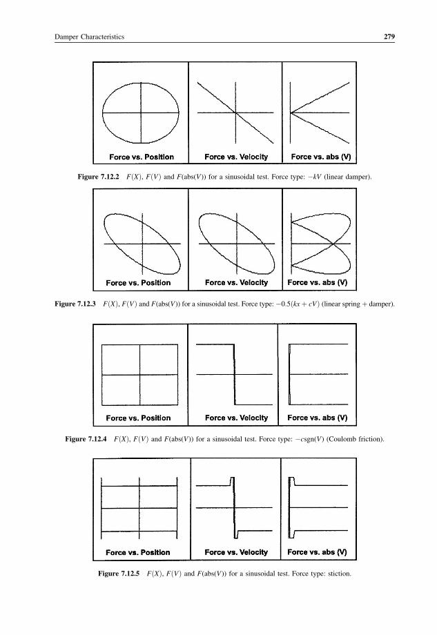
7.12 Cyclical Characteristics, F(X) 278
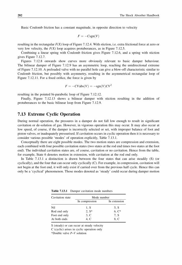
7.13 Extreme Cyclic Operation 282
7.14 Stresses and Strains 283
7.15 Damper Jacking 286
7.16 Noise 287
8 Adjustables 289
8.1 Introduction 289
8.2 The Adjustable Valve 290
8.3 Parallel Hole 294
8.4 Series Hole 294
8.5 Maximum Area 294
8.6 Opening Pressure 294
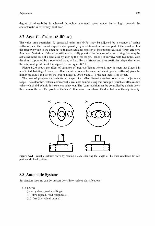
8.7 Area Coefficient (Stiffness) 295
8.8 Automatic Systems 295
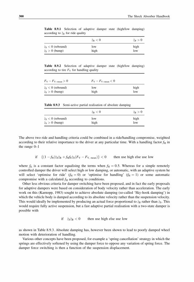
8.9 Fast Adaptive Systems 299
8.10 Motion Ratio 301
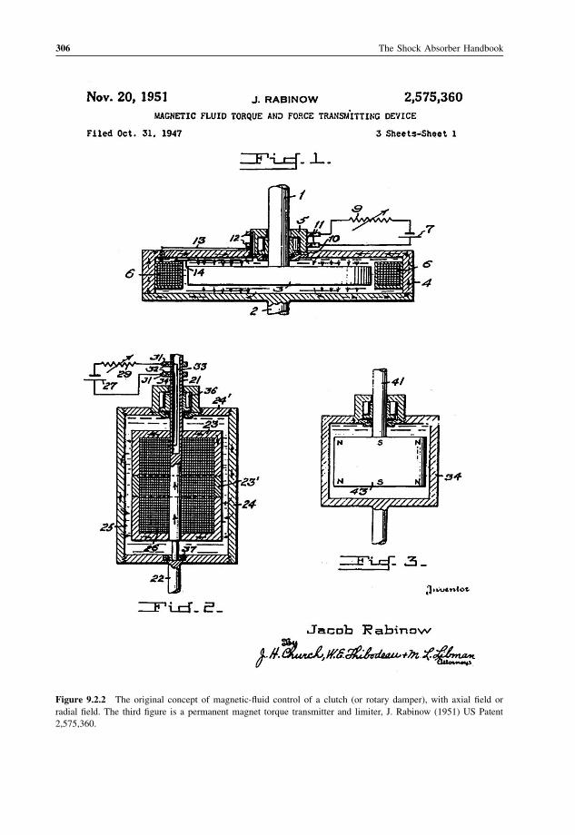
9 ER and MR Dampers 303
9.1 Introduction 303
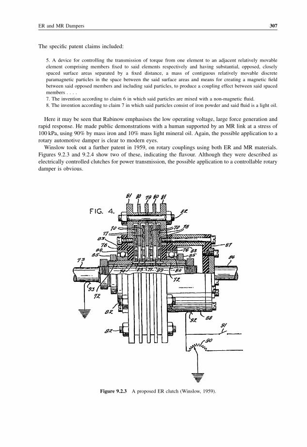
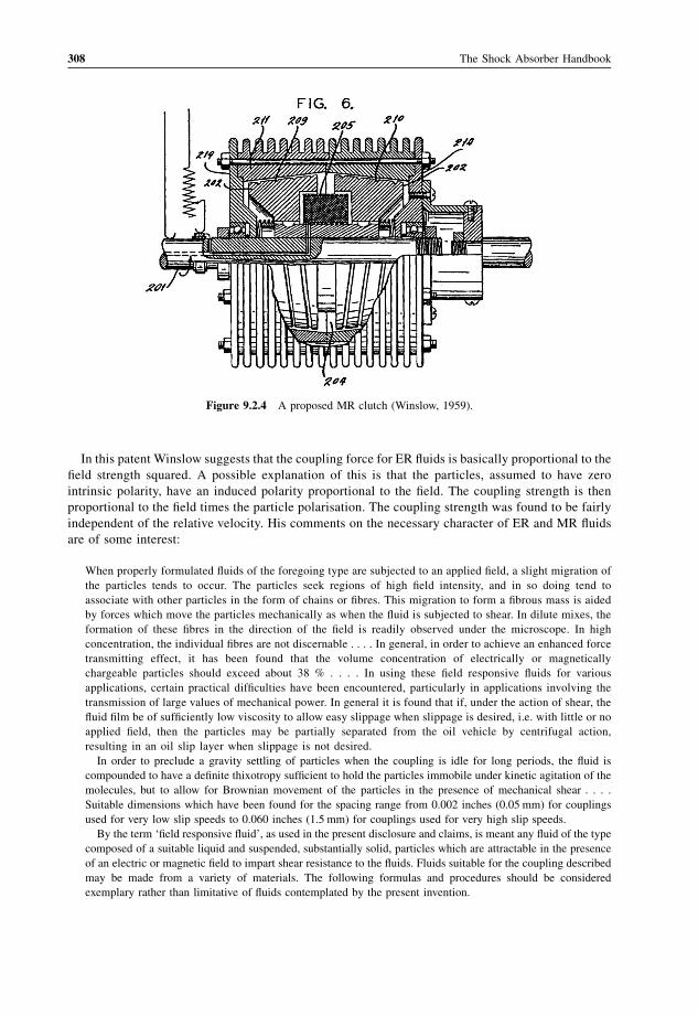
9.2 ER–MR History 303
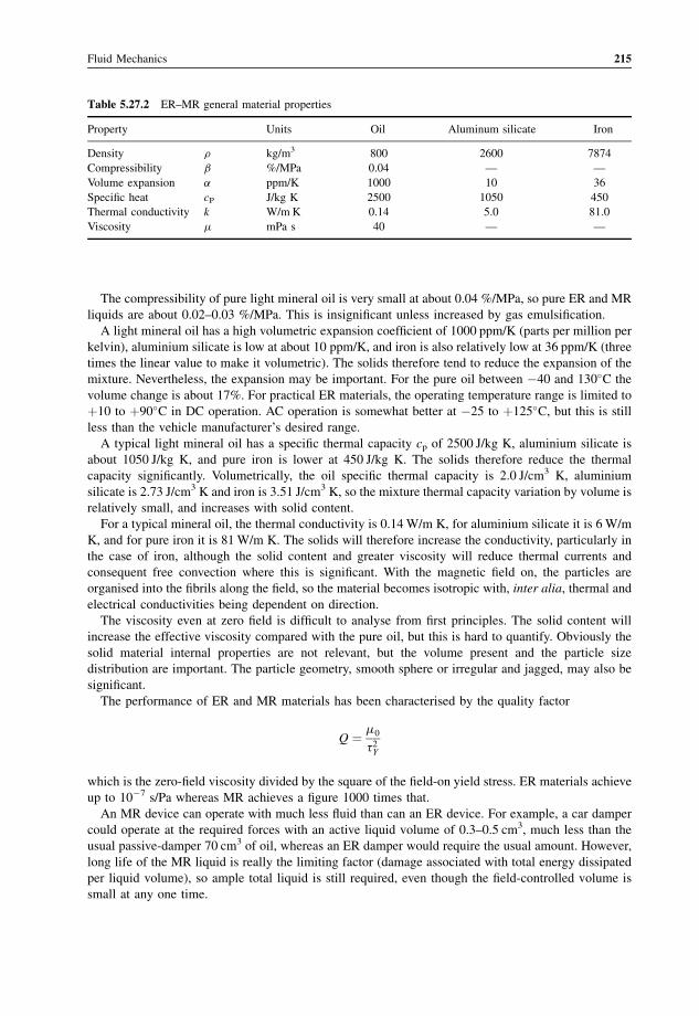
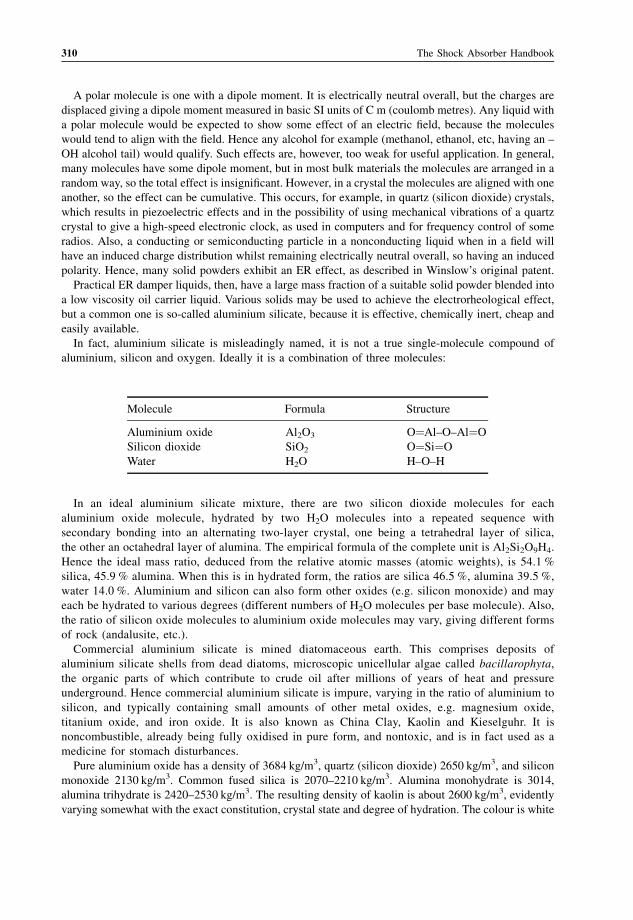
9.3 ER Materials 309
9.4 ER Dampers 314
9.5 ER Controlled Valve 319
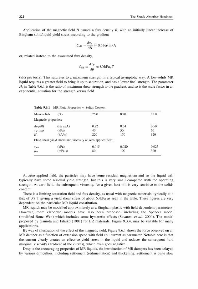
9.6 MR Materials 321
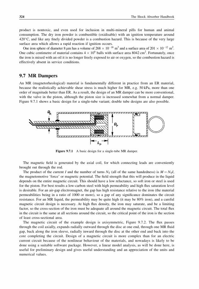
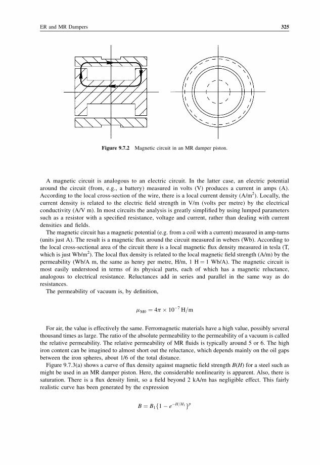
9.7 MR Dampers 324
10 Specifying a Damper 333
10.1 Introduction 333
x Contents
Page 13
10.2 End Fittings 334
10.3 Length Range 334
10.4 F(V) Curve 334
10.5 Configuration 334
10.6 Diameter 335
10.7 Oil Properties 335
10.8 Life 335
10.9 Cost 335
11 Testing 337
11.1 Introduction 337
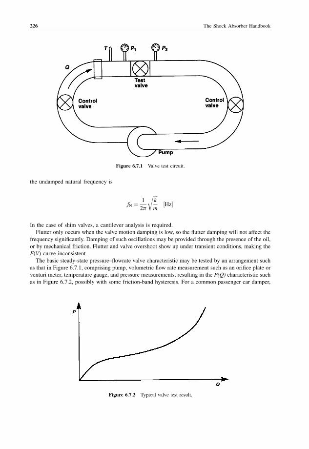
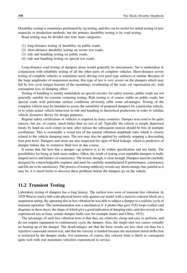
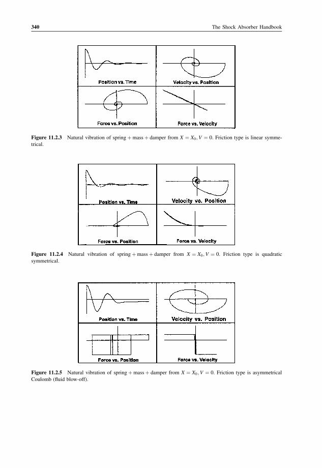
11.2 Transient Testing 338
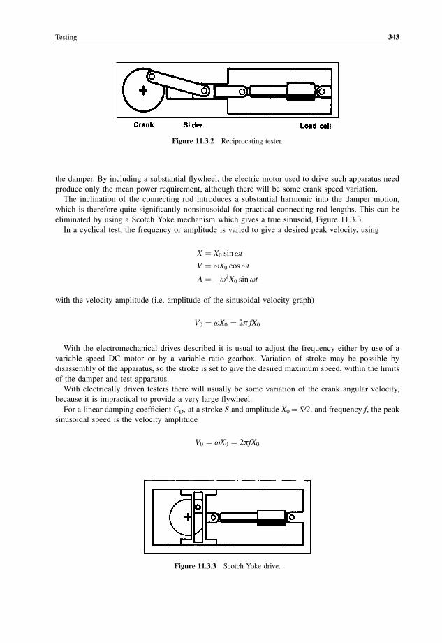
11.3 Electromechanical Testers 342
11.4 Hydraulic Testers 344
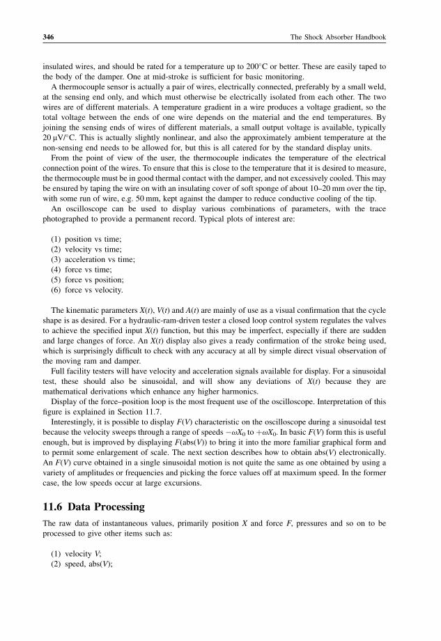
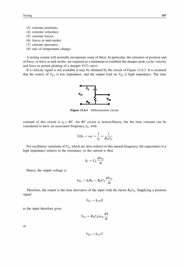
11.5 Instrumentation 345
11.6 Data Processing 346
11.7 Sinusoidal Test Theory 348
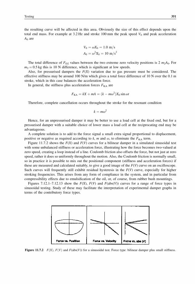
11.8 Test Procedure 352
11.9 Triangular Test 354
11.10 Other Laboratory Tests 356
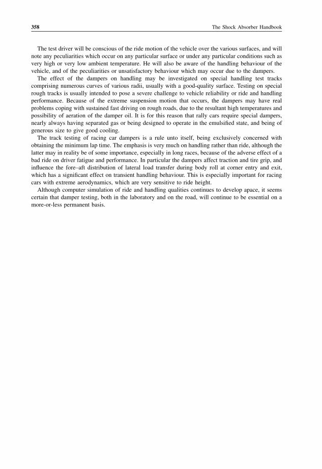
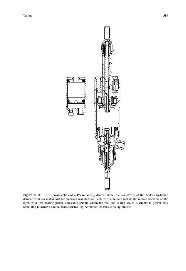
11.11 On-Road Testing 357
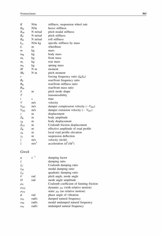
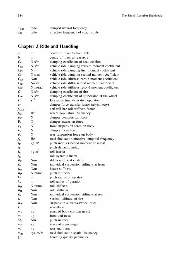
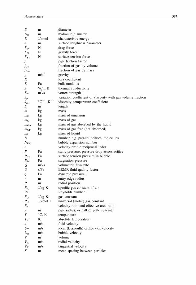
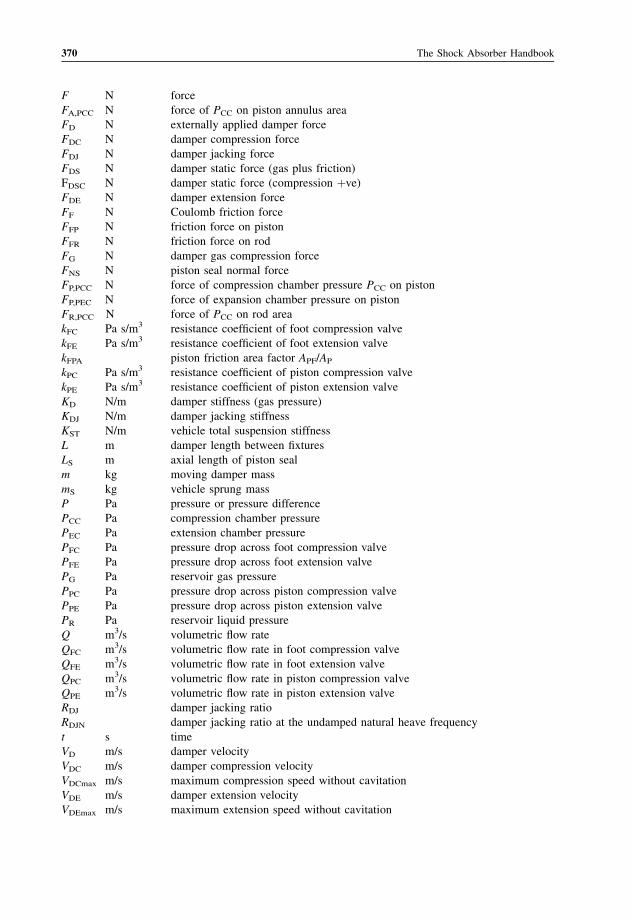
Appendix A: Nomenclature 361
Appendix B: Properties of Air 375
Appendix C: Properties of Water 379
Appendix D: Test Sheets 381
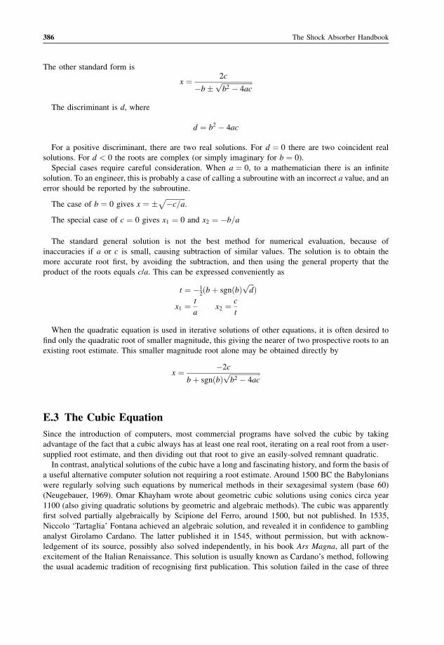
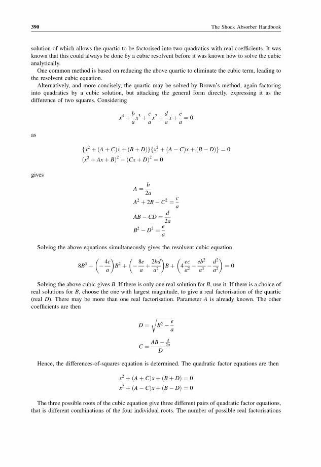
Appendix E: Solution of Algebraic Equations 385
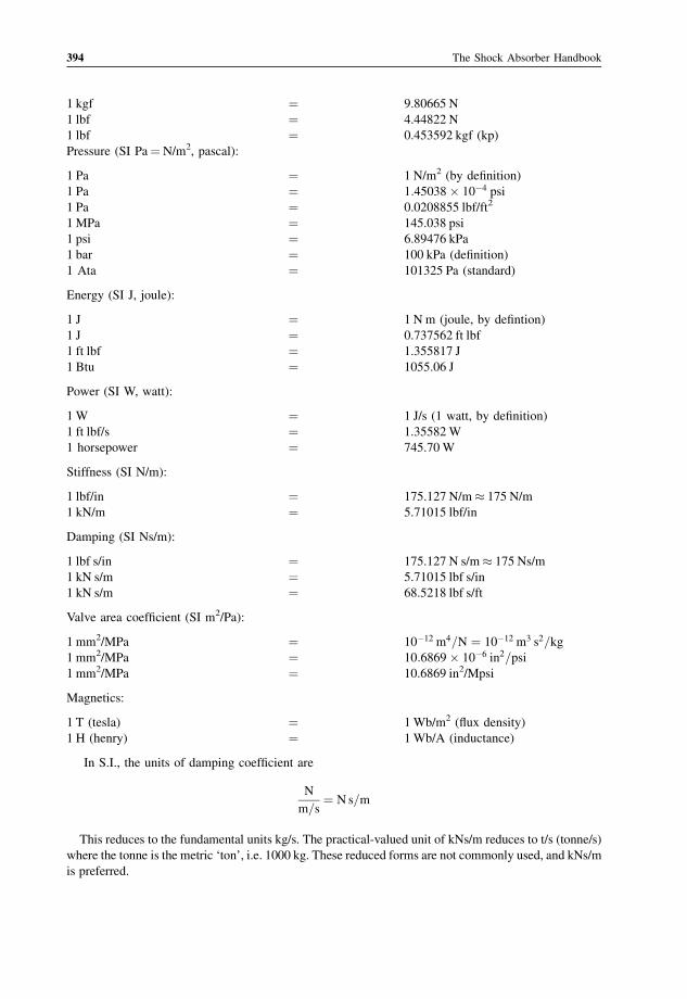
Appendix F: Units 393
Appendix G: Bingham Flow 397
References 401
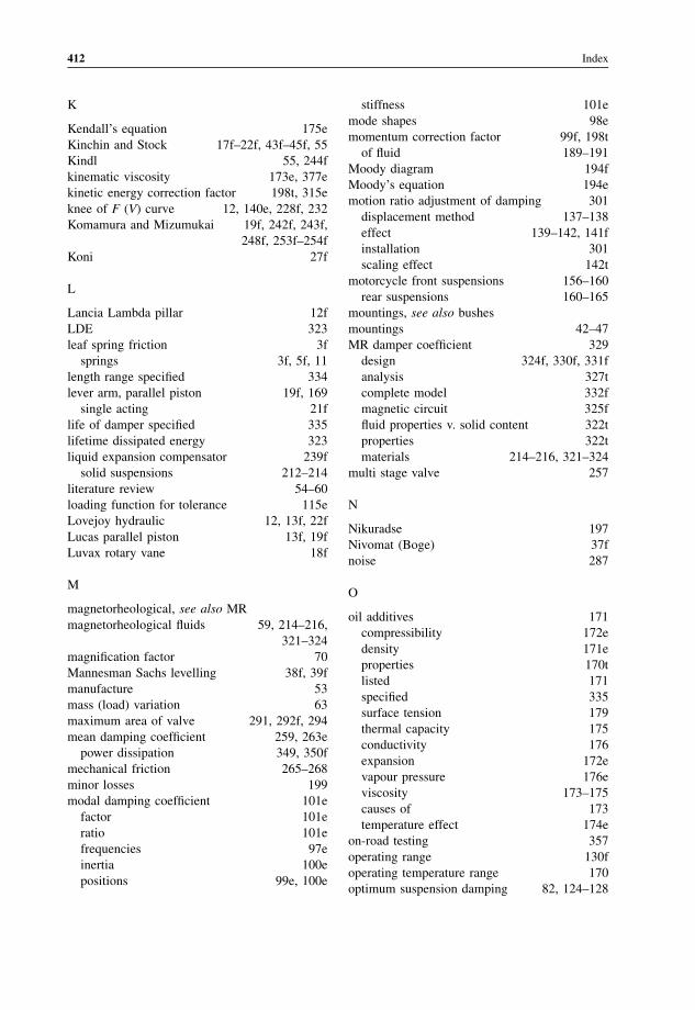
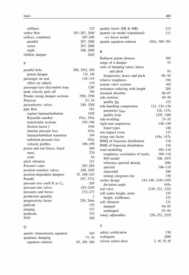
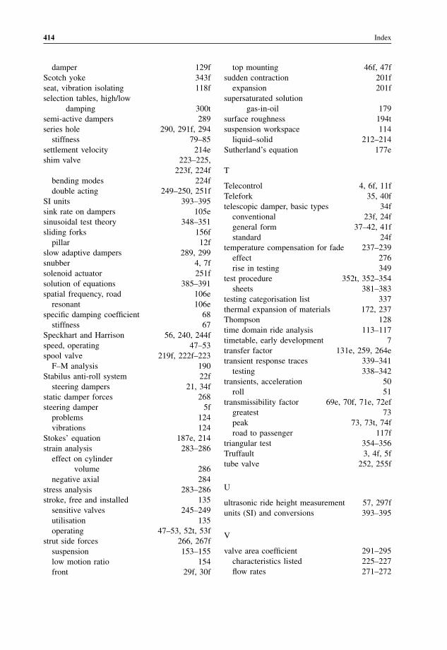
Index 409
Contents xi
Page 15
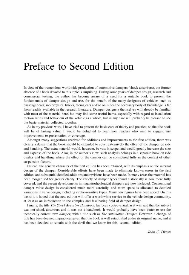
Preface to Second Edition
In view of the tremendous worldwide production of automotive dampers (shock absorbers), the former
absence of a book devoted to this topic is surprising. During some years of damper design, research and
commercial testing, the author has become aware of a need for a suitable book to present the
fundamentals of damper design and use, for the benefit of the many designers of vehicles such as
passenger cars, motorcycles, trucks, racing cars and so on, since the necessary body of knowledge is far
from readily available in the research literature. Damper designers themselves will already be familiar
with most of the material here, but may find some useful items, especially with regard to installation
motion ratios and behaviour of the vehicle as a whole, but in any case will probably be pleased to see
the basic material collected together.
As in my previous work, I have tried to present the basic core of theory and practice, so that the book
will be of lasting value. I would be delighted to hear from readers who wish to suggest any
improvements to presentation or coverage.
Amongst many suggestions received for additions and improvements to the first edition, there was
clearly a desire that the book should be extended to cover extensively the effect of the damper on ride
and handling. The extra material would, however, be vast in scope, and would greatly increase the size
and expense of the book. Also, in the author’s view, such analysis belongs in a separate book on ride
quality and handling, where the effect of the damper can be considered fully in the context of other
suspension factors.
Instead, the general character of the first edition has been retained, with its emphasis on the internal
design of the damper. Considerable efforts have been made to eliminate known errors in the first
edition, and substantial detailed additions and revisions have been made. In many areas the material has
been reorganised for greater clarity. The variety of damper types found historically is now more fully
covered, and the recent developments in magnetorheological dampers are now included. Conventional
damper valve design is considered much more carefully, and more space is allocated to detailed
variations in valve design, including stroke-sensitive types. Many new figures have been added. On this
basis, it is hoped that the new edition will offer a worthwhile service to the vehicle design community,
at least as an introduction to the complex and fascinating field of damper design.
Finally, the title The Shock Absorber Handbook has been controversial, as it was said that the subject
was not shock absorbers and it was not a handbook. It would probably have been better to use the
technically correct term damper, with a title such as The Automotive Damper. However, a change of
title has been deemed impractical given that the book is well established under its original name, and it
has been decided to remain with the devil that we know for this, second, edition.
John C. Dixon
Page 17
Acknowledgements
Numerous figures are reproduced by permission of the Society of Automotive Engineers, The
Institution of Mechanical Engineers, and others. The reference for all previously published figures is
given with the figure.
Page 19
1Introduction
1.1 History
The current world-wide production of vehicle dampers, or so-called shock absorbers, is difficult to
estimate with accuracy, but is probably around 50–100 million units per annum with a retail value
well in excess of one billion dollars per annum. A typical European country has a demand for over
5 million units per year on new cars and over 1 million replacement units, The US market is several
times that. If all is well, these suspension dampers do their work quietly and without fuss. Like
punctuation or acting, dampers are at their best when they are not noticed - drivers and passengers
simply want the dampers to be trouble free. In contrast, for the designer they are a constant interest
and challenge. For the suspension engineer there is some satisfaction in creating a good new damper
for a racing car or rally car and perhaps making some contribution to competition success. Less
exciting, but economically more important, there is also satisfaction in seeing everyday vehicles
travelling safely with comfortable occupants at speeds that would, even on good roads, be quite
impractical without an effective suspension system.
The need for dampers arises because of the roll and pitch associated with vehicle manoeuvring, and
from the roughness of roads. In the mid nineteenth century, road quality was generally very poor. The
better horse-drawn carriages of the period therefore had soft suspension, achieved by using long bent
leaf springs called semi-elliptics, or even by using a pair of such curved leaf springs set back-to-back
on each side, forming full-elliptic suspension. No special devices were fitted to provide damping; rather
this depended upon inherent friction, mainly between the leaves of the beam springs. Such a set-up was
appropriate to the period, being easy to manufacture, and probably worked tolerably well at moderate
speed, although running at high speed must have been at least exciting, and probably dangerous,
because of the lack of damping control.
The arrival of the so-called horseless carriage, i.e. the carriage driven by an internal combustion
engine, at the end of the nineteenth century, provided a new stimulus for suspension development
which continues to this day. The rapidly increasing power available from the internal combustion
engine made higher speeds routine; this, plus the technical aptitude of the vehicle and component
designers, coupled with a general commercial mood favouring development and change, provided an
environment that led to invention and innovation.
The fitting of damping devices to vehicle suspensions followed rapidly on the heels of the arrival of
the motor car itself. Since those early days the damper has passed through a century of evolution, the
basic stages of which may perhaps be considered as:
The Shock Absorber Handbook/Second Edition John C. Dixon
# 2007 John Wiley & Sons, Ltd
Page 20
(1) dry friction (snubbers);
(2) blow-off hydraulics;
(3) progressive hydraulics;
(4) adjustables (manual alteration);
(5) slow adaptives (automatic alteration);
(6) fast adaptives (‘semi-active’);
(7) electrofluidic, e.g. magnetorheological.
Historically, the zeitgeist regarding dampers has changed considerably over the years, in roughly the
following periods:
(1) Up to 1910 dampers were hardly used at all. In 1913, Rolls Royce actually discontinued rear
dampers on the Silver Ghost, illustrating just how different the situation was in the early years.
(2) From 1910 to 1925 mostly dry snubbers were used.
(3) From 1925 to 1980 there was a long period of dominance by simple hydraulics, initially simply
constant-force blow-off, then through progressive development to a more proportional character-
istic, then adjustables, leading to a mature modern product.
(4) From 1980 to 1985 there was excitement about the possibilities for active suspension, which could
effectively eliminate the ordinary damper, but little has come of this commercially in practice so far
because of the cost.
(5) From 1985 it became increasingly apparent that a good deal of the benefit of active suspension
could be obtained much more cheaply by fast auto-adjusting dampers, and the damper suddenly
became an interesting, developing, component again.
(6) From about 2000, the introduction, on high-price vehicles at least, of controllable magnetorheo-
logical dampers.
Development of the adaptive damper has occurred rapidly. Although there will continue to be
differences between commercial units, such systems are now effective and can be considered to be
mature products. Fully active suspension offers some performance advantages, but is not very cost
effective for passenger cars. Further developments can then be expected to be restricted to rather slow
detail refinement of design, control strategies and production costs. Fast acting control, requiring extra
sensors and controls, will continue to be more expensive, so simple fixed dampers, adjustables and slow
adaptive types will probably continue to dominate the market numerically for the foreseeable future.
The basic suspension using the simple spring and damper is not ideal, but it is good enough for most
purposes. For low-cost vehicles, it is the most cost-effective system. Therefore much emphasis remains
on improvement of operating life, reliability and low-cost production rather than on refinement of
performance by technical development. The variable damper, in several forms, has now found quite
wide application on mid-range and expensive vehicles. On the most expensive passenger and sports
cars, magetorheologically controlled dampers are now a popular fitment, at significant expense.
The damper is commonly known as the shock absorber, although the implication that shocks are
absorbed is misleading. Arguably, the shocks are ‘absorbed’ by the deflection of the tires and springs.
The purpose of dampers is to dissipate any energy in the vertical motion of body or wheels, such
motion having arisen from control inputs, or from disturbance by rough roads or wind. Here ‘vertical’
motion includes body heave, pitch and roll, and wheel hop. As an agglomeration of masses and springs,
the car with its wheels constitutes a vibrating system that needs dampers to optimise control behaviour,
by preventing response overshoots, and to minimise the influence of some unavoidable resonances. The
mathematical theory of vibrating systems largely uses the concept of a linear damper, with force
proportional to extension speed, mainly because it gives equations for which the solutions are well
understood and documented, and usually tolerably realistic. There is no obligation on a damper to
exhibit such a characteristic; nevertheless the typical modern hydraulic damper does so approximately.
This is because the vehicle and damper manufacturers consider this to be desirable for good physical
2 The Shock Absorber Handbook
Page 21
behaviour, not for the convenience of the theorist. The desired characteristics are achieved only by
some effort from the manufacturer in the detail design of the valves.
Damper types, which are explained fully later, can be initially classified as
(a) dry friction with solid elements;
(i) scissor;
(ii) snubber;
(b) hydraulic with fluid elements;
(i) lever-arm;
(ii) telescopic.
Only the hydraulic type is in use in modern times. The friction type came originally as sliding discs
operated by two arms, with a scissor action, and later as a belt wrapped around blocks, the ‘snubber’.
The basic hydraulic varieties are lever-arm and telescopic. The lever-arm type uses a lever to operate a
vane, now extinct, or a pair of pistons. Telescopics, now most common, are either double-tube or gas-
pressurised single-tube.
The early days of car suspension gave real opportunities for technical improvement, and financial
reward. The earliest suspensions used leaf springs with inherent interleaf friction. Efforts had been
made to control this to desirable levels by the free curvature of the leaves. Further developments of
the leaf spring intrinsic damping included controlled adjustment of the interleaf normal forces,
Figure 1.1.1, and the use of inserts of various materials to control the friction coefficients, Figure 1.1.2.
Truffault invented the scissor-action friction disc system before 1900, using bronze discs
alternating with oiled leather, pressed together by conical disc springs and operated by two arms,
with a floating body. The amount of friction could be adjusted by a compression hand-screw, pressing
the discs together more or less firmly, varying the normal force at approximately constant friction
coefficient. Between 1900 and 1903, Truffault went on to develop a version for cars, at the instigation
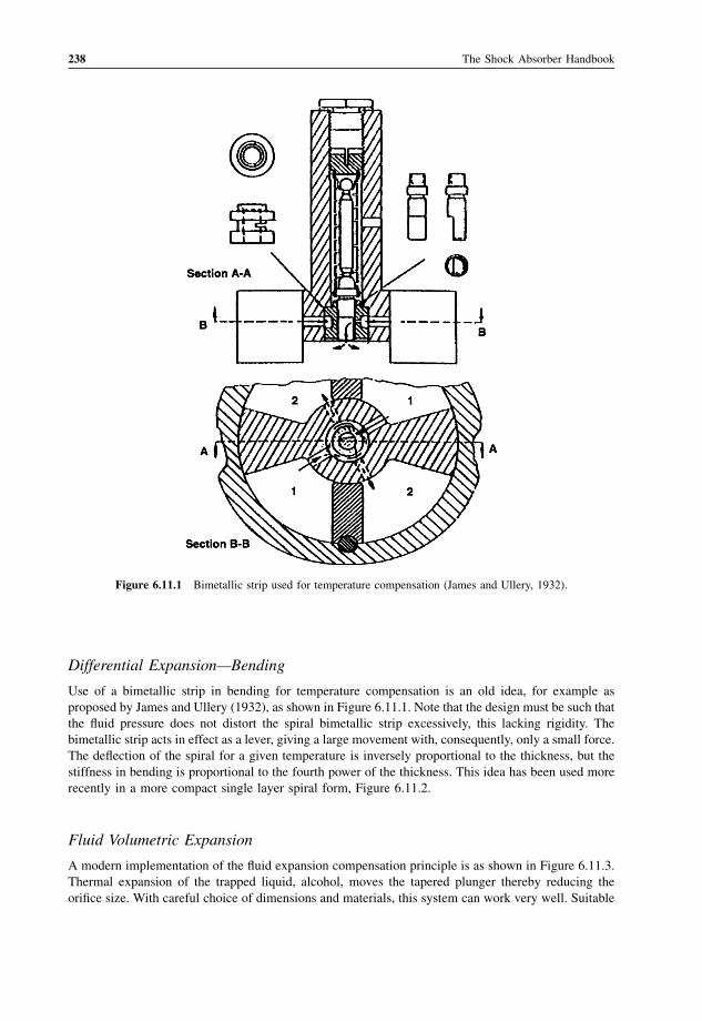
Figure 1.1.1 Dry friction damping by controlled clamping (adjustable normal force) of the leaf spring (Woodhead).
LEADRUBBER
Figure 1.1.2 Leaf spring inserts to control the friction coefficient and consequent damping effect.
Introduction 3
Page 22
of Hartford in the US, who began quantity production in 1904, as in Figures 1.1.3–1.1.5. Truffault,
well aware of the commercial potential, also licensed several other manufacturers in Europe,
including Mors and Peugeot in France, who also had them in production and use by 1904. A similar
type of damper was also pressed into service on the steering, Figure 1.1.6, to reduce steering fight on
rough roads and to reduce steering vibrations then emerging at higher speeds and not yet adequately
understood.
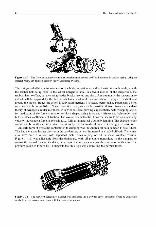
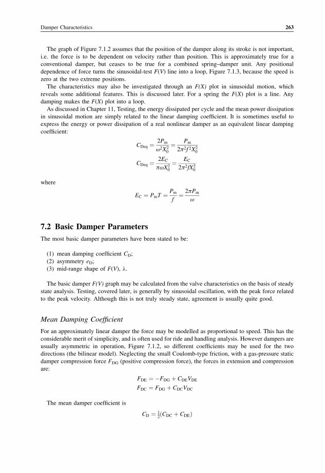
Figure 1.1.7 shows an exploded diagram of a more recent (1950s) implementation from a
motorcycle. This is also adjustable by the hand-screw. Subsequent to the Truffault–Hartford type,
The Hartford Telecontrol (the prefix tele means remote) developed the theme, Figure 1.1.8, with a
convenient Bowden cable adjustment usable by the driver in situ. A later alternative version, the Andre
Telecontrol, had dry friction scissor dampers, but used hydraulic control of the compression force and
hence of the damper friction moment.
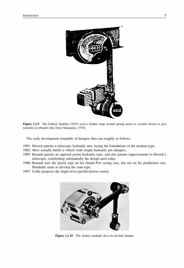
In 1915, Claud Foster invented the dry friction block-and-belt snubber, Figure 1.1.9, manufactured in
very large quantities by his Gabriel company, and hence usually known as the Gabriel Snubber. In view
of the modern preference for hydraulics, the great success of the belt snubber was presumably based on
low cost, ease of retrofitment and reliability rather than exceptional performance.
Figure 1.1.3 An advertisement from 1904 for the early Truffault designed dry friction scissor damper
manufactured by Hartford.
4 The Shock Absorber Handbook
Page 23
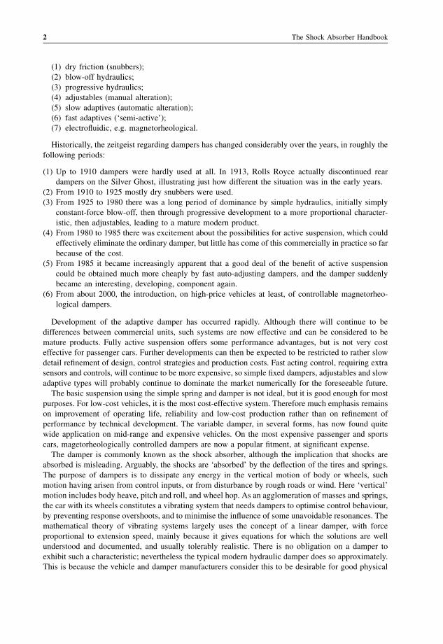
Figure 1.1.4 The Andre–Hartford scissor-action dry friction damper.
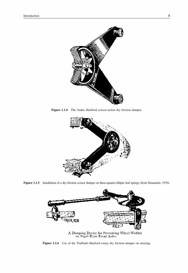
Figure 1.1.5 Installation of a dry-friction scissor damper on three-quarter-elliptic leaf springs (from Simanaitis, 1976).
Figure 1.1.6 Use of the Truffault–Hartford rotary dry friction damper on steering.
Introduction 5
Page 24
The spring-loaded blocks are mounted on the body, in particular on the chassis rails in those days, with
the leather belt being fixed to the wheel upright or axle. In upward motion of the suspension, the
snubber has no effect, but the spring-loaded blocks take up any slack. Any attempt by the suspension to
extend will be opposed by the belt which has considerable friction where it wraps over itself and
around the blocks. Hence the action is fully asymmetrical. The actual performance parameters do not
seem to have been published. Some theoretical analysis may be possible, derived from the standard
theory of wrapped circular members, with friction force growing exponentially with wrapping angle,
for prediction of the force in relation to block shape, spring force and stiffness and belt-on-belt and
belt-on-block coefficients of friction. The overall characteristic, however, seems to be an essentially
velocity-independent force in extension, i.e. fully asymmetrical Coulomb damping. The characteristics
could have been affected in service conditions by the friction-breaking effect of engine vibrations.
An early form of hydraulic contribution to damping was the Andrex oil-bath damper, Figure 1.1.10.
This had metal and leather discs as in the dry damper, but was immersed in a sealed oil bath. There may
also have been a version with separated metal discs relying on oil in shear. Another version,
Figure 1.1.11, was adjustable from the dashboard, with oil pressure transmitted to the dampers to
control the normal force on the discs, or perhaps in some cases to adjust the level of oil in the case. The
pressure gauge in Figure 1.1.11 suggests that this type was controlling the normal force.
Figure 1.1.7 The Greeves motorcycle front suspension from around 1950 had a rubber-in-torsion spring, using an
integral rotary dry friction damper easily adjustable by hand.
Figure 1.1.8 The Hartford Telecontrol damper was adjustable via a Bowden cable, and hence could be controlled
easily from the driving seat, even with the vehicle in motion.
6 The Shock Absorber Handbook
Page 25
The early development timetable of dampers thus ran roughly as follows:
1901: Horock patents a telescopic hydraulic unit, laying the foundations of the modern type.
1902: Mors actually builds a vehicle with simple hydraulic pot dampers.
1905: Renault patents an opposed piston hydraulic type, and also patents improvements to Horock’s
telescopic, establishing substantially the design used today.
1906: Renault uses the piston type on his Grand Prix racing cars, but not on his production cars.
Houdaille starts to develop his vane-type.
1907: Caille proposes the single-lever parallel-piston variety.
Figure 1.1.9 The Gabriel Snubber (1915) used a leather strap around sprung metal or wooden blocks to give
restraint in rebound only (from Simanaitis, 1976).
Figure 1.1.10 The Andrex multiple discs-in-oil-bath damper.
Introduction 7
Page 26
1909: A single-acting Houdaille vane type is fitted as original equipment, but this is an isolated success
for the hydraulic type, the friction disc type remaining dominant.
1910: Oil damped undercarriages come into use on aircraft.
1915: Foster invents the belt ‘snubber’ which had great commercial success in the USA.
1919: Lovejoy lever-arm hydraulic produced in the USA.
1924: Lancia introduces the double-acting hydraulic unit, incorporated in the front independent
pillar suspension of the Lambda. The Grand Prix Bugatti uses preloaded nonadjustable drum-
brake type.
1928: Hydraulic dampers are first supplied as standard equipment in the USA.
1930: Armstrong patents the telescopic type.
1933: Cadillac ‘Ride Regulator’ driver-adjustable five-position on dashboard.
1934: Monroe begins manufacture of telescopics.
1947: Koning introduces the adjustable telescopic.
1950: Gas-pressurised single-tube telescopic is invented and manufactured by de Carbon.
2001: Magnetorheological high-speed adjustables introduced (Bentley, Cadillac).
Figure 1.1.11 The adjustable version of the Andrex oil-bath damper included pump, reservoir and pressure gauge.
8 The Shock Absorber Handbook
Page 27
The modern success of hydraulics over dry friction is due to a combination of factors, including:
(1) Superior performance of hydraulics, due to the detrimental effect of dry Coulomb friction which is
especially noticeable on modern smooth roads.
(2) Damper life has been improved by better seals and higher quality finish on wearing surfaces.
(3) Performance is now generally more consistent because of better quality control.
(4) Cost is less critical than of old, and is in any case controlled by mass production on modern
machine tools.
During the 1950s, telescopic dampers gradually became more and more widely used on passenger
cars, the transition being essentially complete by the late 1950s. In racing, at Indianapolis the hydraulic
vane type arrived in the late 1920s, and was considered a great step forward; the adjustable piston
hydraulic appeared in the early 1930s, but the telescopic was not used there until 1950. Racing cars in
Europe were quite slow to change, although the very successful Mercedes Benz racers of 1954–55 used
telescopics. Although other types are occasionally used, the telescopic hydraulic type of damper is now
the widely accepted norm for cars and motorcycles.
It was far from obvious in early days that the hydraulic type of damper would ultimately triumph,
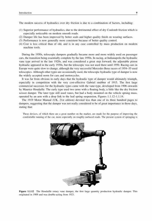
especially in competition with the very cost-effective Gabriel snubber of 1915. The first large
commercial successes for the hydraulic types came with the vane-type, developed from 1906 onwards
by Maurice Houdaille. The early type used two arms with a floating body, a little like the dry friction
scissor damper. The later type still used vanes, but had a body mounted on the vehicle sprung mass,
operated by an arm with a drop link to the leaf spring suspension, Figures 1.1.12–1.1.14.
The 1919 Motor Manual (UK, 21st edition) devoted less than one of its three hundred pages to
dampers, suggesting that the damper was not really considered to be of great importance in those days,
stating that:
These devices, of which there are a great number on the market, are made for the purpose of improving the
comfortable running of the car, more especially on roughly-surfaced roads. The present system of springing is
Figure 1.1.12 The Houdaille rotary vane damper, the first large quantity production hydraulic damper. This
originated in 1909 and was double-acting from 1921.
Introduction 9
Page 28
admittedly not perfect, and when travelling on rough roads there is the objectionable rebound of the body after it
passes over a depression in the road, which it is desirable should be reduced as much as possible. The shock from
this rebound is not only uncomfortable for the passengers, but it has a bad effect on the whole car. Hence these
shock absorbers are applied as the best means available so far to check the rebound. They are made on various
principles, generally employing a frictional effect such as is obtainable from two hardened steel surfaces in close
contact. Another principle is that of using the fluid friction of oil, practically on the lines of any of the well-
known dash-pot devices, viz., a piston moving in a cylinder against the resistance offered by the oil contained
within it, the oil passing slowly through a small aperture into another chamber. This type of device is probably
the best solution of the problem.
Up to 1920 hydraulic dampers were single acting, in droop only, but from 1921 a more complex
valve system allowed some damping in bump too. At this point the operating characteristics of the
Figure 1.1.13 Cross-section of slightly different version of Houdaille rotary vane damper (from Simanaitis, 1976).
Figure 1.1.14 An early configuration of hydraulic damper, a rotary vane device with a drop arm to the axle. Note
the wooden chassis rail (artist’s impression, The Motor Manual, 1919).
10 The Shock Absorber Handbook
Page 29
hydraulic damper had largely reached their modern form. More recent developments have had more to
do with the general configuration, so that the lever-operated type has given way to the telescopic piston
type which is cost-effective in manufacture, being less critical with regard to seal leakage, and has
better air cooling, although lacking the conduction cooling of a body-mounted lever-arm damper. Most
importantly perhaps, the telescopic type lends itself well to the modern form of suspension in terms of
its mounting and ease of installation.
The 1939 Motor Manual (UK, 30th edition), devoted three pages to dampers, perhaps indicating the
increased recognition of their importance for normal vehicles. An illustration was included of the
Andre–Hartford dry friction scissor, and also one of the Luvax vane damper, shown later. There was
also a diagram of the hydraulically adjusted, but dry action, version of the Andre Telecontrol system, as
seen in Figure 1.1.15. That writer was moved to offer some additional explanation of damping and
‘shock absorbing’ in general, stating that:
Whatever form of springing is employed, it is always considered necessary to damp the suspension by
auxiliaries, which have become known as shock absorbers. This term is unfortunate, because it is the function of
the springs to absorb shocks, whereas the ‘shock absorbers’ serve the purpose of providing friction in a
controlled form which prevents prolonged bouncing or pitching motions, by absorbing energy. A leaf spring is
inherently damped by the friction between the leaves, and it may, therefore, seem strange that after lubricating
these leaves friction should be put back into the system by the use of shock absorbers. The explanation is that
leaf friction is not readily controllable, whereas the shock absorber imparts a definite and adjustable degree of
damping to the system.
The most popular type of shock absorber is an hydraulic device which is bolted to the frame and is operated by
an arm coupled to the axle. Four such devices are ordinarily fitted. When relative movement occurs between the
axle and the frame, the arm on the shock absorber spindle is oscillated, and this motion is conveyed to a rotor,
which fits within a circular casing. Oil in the casing in made to flow through valves from one side of the rotor to
the other and so creates hydraulic resistance which damps the oscillations. In some cases the valves are arranged
to give ‘double action’, the damping then being effective on both deflection and rebound. In other cases
single-acting devices are used which can check rebound only. As a rule the action of the shock absorbers can be
adjusted by means of a screw, which alters the tension of a spring and so varies the load on a ball valve.
Figure 1.1.15 Layout of the hydraulically remote Andre Telecontrol damper, shown here on a front axle (The
Motor Manual, 1939).
Introduction 11
Page 30
The hydraulic shock absorber has the important merit of increasing its damping effect when subject to sudden
movements, but suffers from the defect of providing very little resistance against slower motions, such as rolling.
Consequently, for sports cars many users prefer frictional shock absorbers, of the scissor (constant resistance)
type, of which the most famous is the Andre–Hartford.
The final comment above is significant in a modern context, regarding the preferred velocity–force
relationship, which is a regressive shape with a ‘knee’, rather than simply linear.
The Lancia Lambda of 1925 had sliding pillar suspension, Figure 1.1.16, now almost extinct
(except, e.g. Morgan) and regarded as primitive, but highly successful at the time. It was noted for
the fact that its oil-filled cylinders required no maintenance, and was very reliable. This is an
attractive option for a light vehicle, because it is such a compact and light system, although lacking
the ability of modern suspensions to be adjusted to desired handling characteristics by detailed
changes to the geometry.
Although dry friction snubbers remained in wide use through to the 1930s, hydraulic fluid-based
dampers were in limited use from very early days and continued to grow in popularity. An early
successful version in the USA was made by Lovejoy, Figure 1.1.17.
Difficulties with sealing and wear of vane lever arm types led to the lever arm parallel piston system
as in the Lovejoy and in the Armstrong, Figure 1.1.18, in which the valve may also easily be made
Figure 1.1.16 The Lancia Lambda sliding-pillar system had the spring and damper sealed into one unit (Lancia,
1925).
12 The Shock Absorber Handbook
Page 31
interchangeable. This would still be a usable design today. Some economy of parts may be achieved by
lengthening the bearing and using the lever as the load-carrying suspension arm, Figure 1.1.19. This
can be taken further by putting the axle in double shear, so that the lever becomes an A-arm
(wishbone), Figure 1.1.20.
Figure 1.1.17 The Lovejoy lever-arm hydraulic damper, first produced in 1919.
Figure 1.1.18 The double parallel-piston damper was the ultimate lever-arm configuration, overcoming the
problems of the vane lever-arm type (Lucas) (see also Figure 1.3.7).
Introduction 13
Page 32
However, despite the many creative innovations in lever arms, it seems that the telescopic is now
almost universally preferred. At the front this has become the ubiquitous telescopic strut, partly
because of the convenience of final assembly.
Figure 1.1.19 The simple lever-arm damper can be reinforced to carry suspension loads by lengthening the
bearing rod.
Figure 1.1.20 The A-arm (wishbone) suspension arm is lighter than a single arm when large loads are to be
resisted, and adapts well to a double-shear connection to a lever-arm damper.
14 The Shock Absorber Handbook
Page 33
An interesting development was the Armstrong ‘double telescopic lever arm’, Figure 1.1.21, in which
two telescopic dampers operate horizontally, fully immersed in an oil bath, with an external structure
like a conventional lever arm type. Possibly this was done to combine the Armstrong-type telescopic
into a unit that could be used interchangeably with its lever-arm competitors. An advantage of this
layout over a plain telescopic is that any amount of damping is easily arranged in compression and
rebound independently, with each damper of the pair acting in one direction only, without concern for
oil cavitation.
As a final remark on the very early historical development, it may be noted that the dry friction
scissor damper and the snubber were remarkably persistent. They were light in weight and low in cost,
and perhaps more reliable than the early vane hydraulics which probably suffered from quality control
problems and oil leakage. The parallel-piston lever-arm damper was functionally very good, and the
fact that it has been superseded by the hydraulic telescopic, and the strut in particular at the front, is
mainly due to the final assembly advantages of these, rather than any functional gain in the areas of ride
and handling. In steering, the rack system has a better reputation than the old steering boxes, but it is
hard, if not impossible, to tell the difference in practice. Similarly, the triumph of the telescopic damper
system is not simply due to technical deficiencies of the older systems. The popular new direct
acting telescopics that were ultimately to dominate were typified by the Woodhead–Monroe as in
Figure 1.1.22.
1.2 Types of Friction
The purpose of a damper, or so-called ‘shock absorber’, is to introduce controlled friction into the
suspension system. In this context, it is possible to identify three distinct types of friction:
(1) dry solid friction;
(2) fluid viscous friction;
(3) fluid dynamic friction.
Any of these types may be used to give suspension damping, but their characteristics are totally
different.
Dry solid friction between ordinary hard materials has a maximum shear friction force which is
closely proportional to the normal force at the surface:
FF � mFFN
Figure 1.1.21 The Armstrong ‘double telescopic lever arm’ damper.
Introduction 15
Page 34
where mF is the coefficient of limiting friction. For hard materials this is approximately constant over a
good range of FN, and relatively independent of the contact area. This is called Coulomb friction.
However it is generally sensitive to temperature, reducing as this increases. Also it is sensitive to the
sliding velocity in an undesirable way. For analysis it is common practice to consider there to be a static
coefficient of friction mS available before any sliding occurs, and a dynamic value mD once there is
relative motion. The dynamic value is lower, perhaps 70% of the static value.
Coulomb friction is undesirable in a suspension, provided that there is sufficient friction of desirable
type, because it locks the suspension at small forces, and gives a poor ride on smooth surfaces, once
known in the USA by the colourful term ‘Boulevard Jerk’. Hence, nowadays, in order to optimise ride
quality every effort is made to minimise the Coulomb friction, including the use of rubber bushes rather
than sliding bushes at suspension pivot points.
Fluid friction is considered in detail in a later chapter, but basically viscous friction is proportional to
the flow rate, and in this sense is an attractive option. Unfortunately, fluid viscosity is very sensitive
to temperature. Fluid dynamic friction, arising with energy dissipation from turbulence, is proportional
Figure 1.1.22 Cross-section of a typical telescopic damper showing the general features, shown without the dust
shroud (Woodhead–Monroe).
16 The Shock Absorber Handbook
Page 35
to the flow rate squared, which is undesirable because it gives forces too high at high speed or too low
at low speed. However it depends on the fluid density rather than the viscosity, so the temperature
sensitivity, although not zero, is much less than for viscous damping.
Much of the subtlety of damper design therefore hinges around obtaining a desirable friction
characteristic which is also consistent, i.e. not unduly sensitive to temperature. This is achieved by
using the fluid-dynamic type of friction, with pressure-sensitive variable-area valves to give the desired
variation with speed.
1.3 Damper Configurations
There have been numerous detailed variations of the hydraulic damper. The principal types may be
classified as:
(1) lever vane (e.g. Houdaille);
(2) lever cam in-line pistons (e.g. Delco Lovejoy);
(3) lever cam parallel pistons, (e.g. Delco);
(4) lever rod piston (e.g. Armstrong);
(5) telescopic.
These and some other types are further illustrated by the variety of diagrams in Figures 1.3.1–1.3.29.
Figure 1.3.1 Double-acting vane type damper (Fuchs, 1933).
Figure 1.3.2 Early vane-type damper (Kinchin and Stock, 1951/1952).
Introduction 17
Page 36
Figure 1.3.3 The Luvax rotary vane hydraulic damper, which featured thermostatic compensation of variation of
oil properties. This was a genuine improvement on earlier vane types. The vane shape results in a radial force that
takes up any freedom in the bearing in a way that minimises vane leakage (The Motor Manual, 1939).
Figure 1.3.4 Lever-operated piston-type damper with discharge to recuperation space (Reproduced from Kinchin
and Stock (1951) pp. 67–86 with permission).
Figure 1.3.5 Lever-operated piston-type damper with pressure recuperation (Reproduced from Kinchin and Stock
(1951) pp. 67–86 with permission).
18 The Shock Absorber Handbook
Page 37
Most passenger cars now have struts at the front. These combine the damping and structural functions,
with an external spring. The main advantage, compared with double wishbones, is fast assembly line
integration of pre-prepared assemblies. There are some disadvantages. The main rod must be of large
diameter to give sufficient rigidity and bearing surface to accept running and cornering loads. The
piston is subject to side loads, and must have a large rubbing area. These tend to add Coulomb friction.
The top strut mounting must transmit the full vertical suspension force, so it is less easy to put a good
compliance in series with the damper. The large dimensions mean larger oil flow rates and less critical
valves, although wear may still be a problem in some cases.
Gas springing has been used for many years, two of the main exponents in passenger cars being
Citroen and British Leyland/BMC/Austin/Morris. The gas is lighter than a metal spring, but requires
containment. The damping function is then integrated with the spring units, as in Figure 1.3.22 et seq.
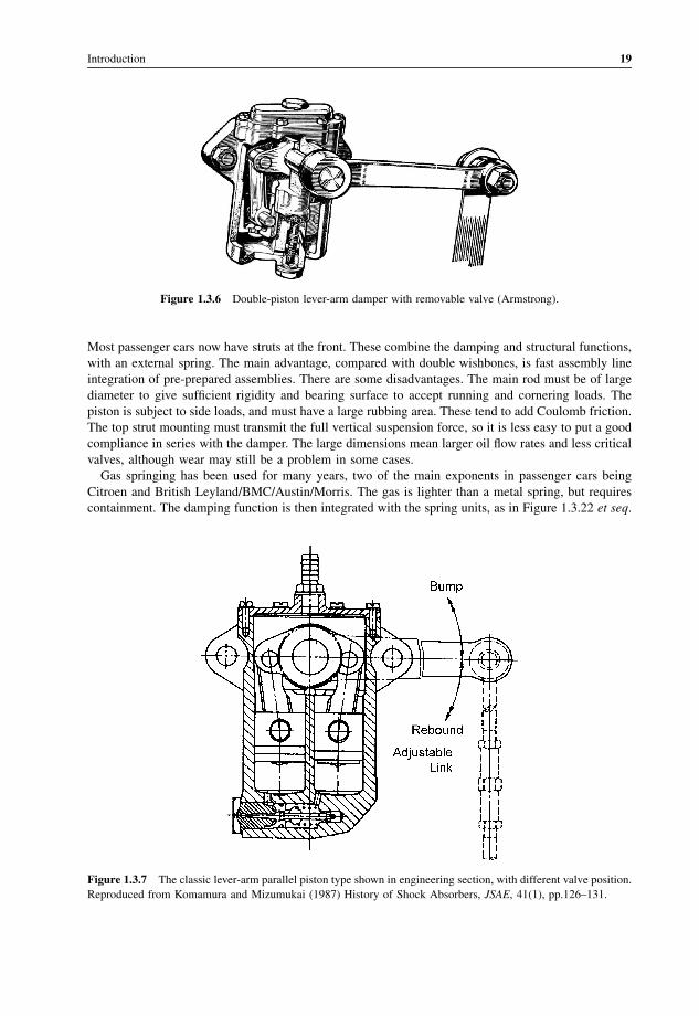
Figure 1.3.6 Double-piston lever-arm damper with removable valve (Armstrong).
Figure 1.3.7 The classic lever-arm parallel piston type shown in engineering section, with different valve position.
Reproduced from Komamura and Mizumukai (1987) History of Shock Absorbers, JSAE, 41(1), pp.126–131.
Introduction 19
Page 38
Front-to-rear interconnection allows reduction of the pitch frequency, which is particularly useful on
small cars. BMC used simple rubber suspensions with separate dampers, and Hydrolastic and Hydragas
with integrated damping.
The most common form of adjustable damper has a rotary valve with several positions each having a
different orifice size. Some form of rotational position control, e.g. a stepper motor, is fixed to the top,
controlling the piston valve through a shaft in the hollow rod, as seen in Figure 1.3.25. The more recent
type uses magneto-rheological liquid, and is discussed separately.
Figure 1.3.8 Lever-operated parallel-piston type damper with valves in the pistons (Reproduced from Kinchin and
Stock (1951) pp. 67–86 with permission).
Figure 1.3.9 Double-telescopic lever-arm configuration showing details for standard fixed valve and for the
manually adjustable in situ version (Armstrong).
20 The Shock Absorber Handbook
Page 39
Steering dampers are much smaller and lighter duty units, and usually operate in the horizontal
position. Double tube dampers are not practical in this role. Figures 1.3.26 and 1.3.27 show two
versions. In the first, the rod volume and oil thermal expansion are catered for by a spring-loaded free
piston. In the second, there is an equalisation chamber having an elastic tube. This separates the oil and
the gas, instead of a piston, reducing leakage problems.
In summary of vehicle damper types, then, the vane type is rarely used nowadays because the
long seal length is prone to leakage and wear, and it therefore requires very viscous oil which
increases the temperature sensitivity. The various lever and piston types are occasionally still used,
but the construction implies use of a short piston stroke (in effect an extreme value of motion ratio),
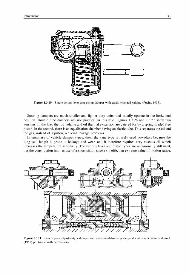
Figure 1.3.10 Single-acting lever-arm piston damper with easily changed valving (Fuchs, 1933).
Figure 1.3.11 Lever-operated piston-type damper with end-to-end discharge (Reproduced from Kinchin and Stock
(1951) pp. 67–86 with permission).
Introduction 21
Page 40
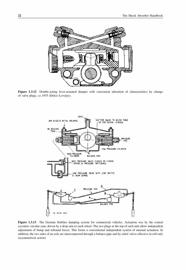
Figure 1.3.12 Double-acting lever-actuated damper with convenient alteration of characteristics by change
of valve plugs, ca 1935 (Delco–Lovejoy).
Figure 1.3.13 The German Stabilus damping system for commercial vehicles. Actuation was by the central
eccentric circular cam, driven by a drop arm to each wheel. The two plugs at the top of each unit allow independent
adjustment of bump and rebound forces. This forms a conventional independent system of unusual actuation. In
addition, the two sides of an axle are interconnected through a balance pipe and by relief valves effective in roll only
(asymmetrical action).
22 The Shock Absorber Handbook
Page 41
Figure 1.3.14 Parts of typical conventional telescopic damper of 1950. Note the four-coil air/oil separation rod in
the reservoir to discourage the effects of agitation. Reproduced from Peterson (1953) Proc. National Conference on
Industrial Hydraulics, 7, 23–43.
Introduction 23
Page 42
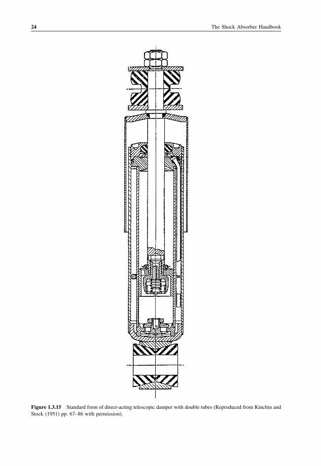
Figure 1.3.15 Standard form of direct-acting telescopic damper with double tubes (Reproduced from Kinchin and
Stock (1951) pp. 67–86 with permission).
24 The Shock Absorber Handbook
Page 43
so the forces and pressures need to be very high. Again this can create sensitivity to leakage. The lever
types have the advantage that the damper body can be bolted firmly to the vehicle body, assisting with
cooling. Another advantage is that there is no internal volume change due to the motion.
However, the lever type has now been almost entirely superseded by the telescopic type, which
has numerous detail variations, and may be classified in several ways. The main classification
concerns the method by which the insertion volume of the rod is accommodated. This is a major
design problem because the oil itself is nowhere near compressible enough to accept the internal
volume reduction of 10% or more associated with the full stroke insertion. Although this
displacement volume seems to be a major disadvantage of the telescopic damper compared with
the lever type, even the lever arm damper must allow for thermal expansion of the oil, which is
significant, so the disadvantage in this respect is not great.
There are three basic telescopic types, as in Figure 1.3.28:
(1) the through-rod telescopic;
(2) the double-tube telescopic;
(3) the single-tube telescopic.
Figure 1.3.16 DeCarbon type of telescopic damper with floating secondary (‘sealing’) piston and high pressure in
the gas chamber. The secondary piston must have sufficient free movement to accommodate the rod displacement
volume and oil thermal expansion. A disadvantage is that the main rod seal is continuously subject to high pressure
so good manufacturing quality is required to prevent long-term leakage. Also, in some applications (off road), the
single tube is prone to damage.
Introduction 25
Page 44
The through-rod telescopic avoids the displacement volume difficulty by passing the rod right
through the cylinder. However this has several disadvantages; there are external seals at both ends
subject to high pressures, the protruding free end may be inconvenient or dangerous, and there is still
no provision for thermal expansion of the oil. However it is a simple solution which has the merit that it
can be used in any orientation. This type has proved impractical for suspension damping, but is
sometimes used for damping of the steering.
In the double-tube type of telescopic, a pair of concentric tubes are used, the exterior annulus
containing some gas to accommodate the rod displacement volume. Hence it must be used the correct
way up. In the single-tube type, some gas may be included, which normally forms an emulsion with the
oil; alternatively the gas is separated by an independent floating piston (de Carbon type) as shown in
Figure 1.3.17 To eliminate the free piston, an emulsified oil may be used, distributing the expansion and rod-
accommodation volume throughout the main oil volume. Overall length is reduced. On standing, the gas separates,
but quickly re-emulsifies on action. The valves must be rated to allow for the passage of emulsion rather than liquid
oil (Woodhead).
26 The Shock Absorber Handbook
Page 45
Figure 1.3.28 (c). The rod is usually fitted with a shroud, of metal or plastic, or possibly a rubber boot,
to reduce the amount of abrasive dirt depositing on the rod, which otherwise may cause premature
seal wear.
Any internal pressure acts on the rod area to give a suspension force, normally lifting the vehicle.
Such pressurisation is avoided as far as possible in the double-tube damper, which minimises leakage.
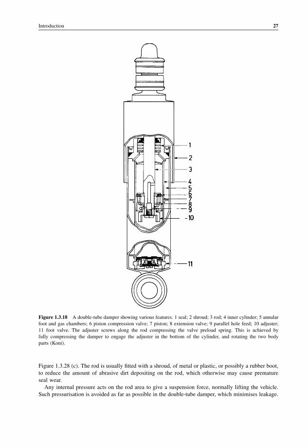
Figure 1.3.18 A double-tube damper showing various features. 1 seal; 2 shroud; 3 rod; 4 inner cylinder; 5 annular
foot and gas chambers; 6 piston compression valve; 7 piston; 8 extension valve; 9 parallel hole feed; 10 adjuster;
11 foot valve. The adjuster screws along the rod compressing the valve preload spring. This is achieved by
fully compressing the damper to engage the adjuster in the bottom of the cylinder, and rotating the two body
parts (Koni).
Introduction 27
Page 46
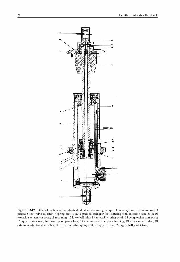
Figure 1.3.19 Detailed section of an adjustable double-tube racing damper. 1 inner cylinder; 2 hollow rod; 3
piston; 5 foot valve adjuster; 7 spring seat; 8 valve preload spring; 9 foot sintering with extension feed hole; 10
extension adjustment point; 11 mounting; 12 lower ball joint; 13 adjustable spring perch; 14 compression shim pack;
15 upper spring seat; 16 lower spring perch lock; 17 compression shim pack backing; 18 extension chamber; 19
extension adjustment member; 20 extension valve spring seat; 21 upper fixture; 22 upper ball joint (Koni).
28 The Shock Absorber Handbook
Page 47
Figure 1.3.20 Sectional view of a front strut for a small car. Piston diameter 27 mm, rod diameter 20 mm. 1 outer
cylinder; 2 spring seat; 3 guard; 4, 5 wheel hub fixture; 6 rolled closure; 7, 8 bump stop seat; 9 seal; 10 upper
moulding; 11 bearing; 12 rod; 13 stroke limiter (?); 14 inner (working) cylinder; 15 piston (Fiat/Monroe).
Introduction 29
Page 48
Figure 1.3.21 Sectional view of a front strut for a larger car. Piston diameter 36 mm, rod diameter 22 mm. 1 rod;
2 seal; 3 bush; 4 rolled closure; 5 bush; 6 top moulding; 7 bearing bush; 8 sleeve; 9 gas chamber; 11 centre
moulding; 12 hole; 13 seal; 14 impact guard; 15 piston; 16 compression chamber; 17 inner (working) cylinder; 18
annular foot chamber; 19 wheel hub fixture; 20 foot valve (Boge).
30 The Shock Absorber Handbook
Page 49
The pressurised single-tube type may suffer from loss of pressure with failure of correct function in
compression due to cavitation behind the piston.
Suda et al. (2004) have proposed a nonhydraulic EM (electromagnetic) damper, of general
configuration as in Figure 1.3.29. Actuation of the EM damper rotates the ball screw nut which drives
an electrical generator through a planetary gearbox. An alternative arrangement uses a rack and pinion
for the mechanical drive. The obvious advantage of an EM damper is controllability—the damper force
depends on the generator and its electrical load. An external power supply is not needed, because the
damper can generate its own electrical supply. A suggestion that energy from suspension motions can
usefully be recovered to save fuel seems optimistic, as the average damper power dissipation is only
a few watts for the whole vehicle. The Suda prototype successfully demonstrated appropriate
characteristics with a damping coefficient around 1.6 kN s/m, and was tested with encouraging
performance on the rear of a passenger car. The concept is an interesting alternative to ER and MR
dampers, but it remains to demonstrate its life and manufacturing economics.
Figure 1.3.22 Citroen air suspension. The valve, with two shim pack valves, is fixed in position. It is not in the
piston, which ideally would pass no oil. The gas is held in the elastomeric rolling seal bag. Nitrogen is used,
reducing oxidation ageing of the rubber.
Introduction 31
Page 50
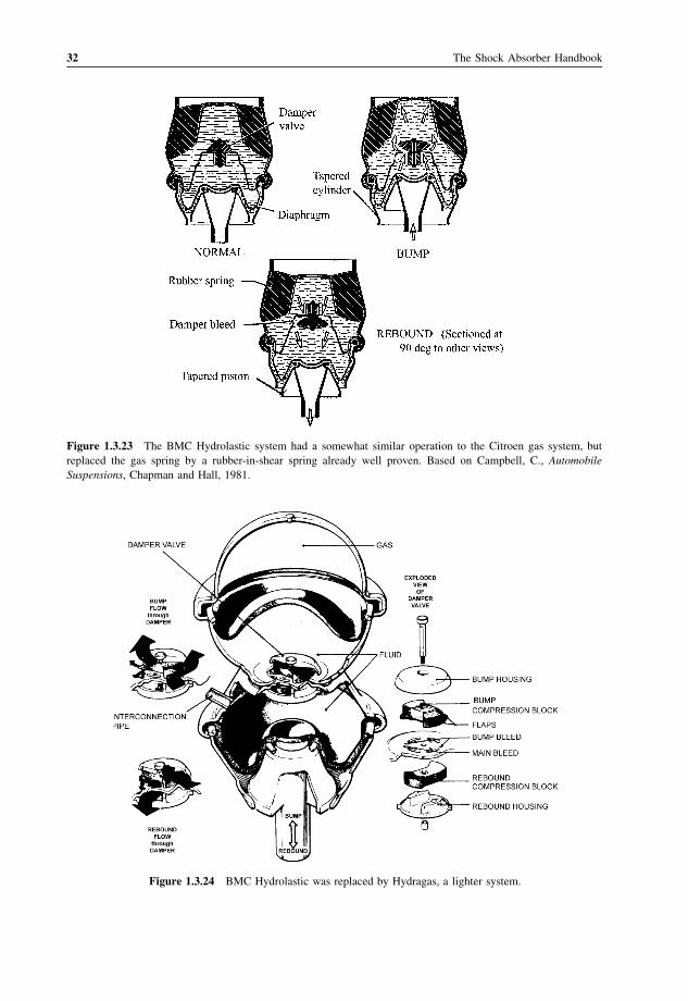
Figure 1.3.23 The BMC Hydrolastic system had a somewhat similar operation to the Citroen gas system, but
replaced the gas spring by a rubber-in-shear spring already well proven. Based on Campbell, C., Automobile
Suspensions, Chapman and Hall, 1981.
Figure 1.3.24 BMC Hydrolastic was replaced by Hydragas, a lighter system.
32 The Shock Absorber Handbook
Page 51
1.4 Ride-Levelling Dampers
One common problem with vehicles is that the load variation is a significant fraction of the kerb
weight, perhaps 40%, particularly for small cars. This causes variation of the suspension
performance with load condition. Many efforts have been made to overcome this. The most
basic factor is the ride height, which varies, in particular at the rear. The telescopic damper offers
the obvious possibility of making compensating adjustments to restore the ride height by simple
pressurisation, Figures 1.4.1–1.4.5 illustrate some efforts along these lines. The operation of a self-
levelling system can be very slow acting without detriment, so the pump may be very low power. It
Figure 1.3.25 An electrically controlled adjustable damper. In this example, the basic construction is a single tube
de Carbon configuration (Bilstein).
Introduction 33
Page 52
Figure 1.3.26 Steering damper of basic de Carbon layout, having a free piston separating the oil from the gas
chamber, but with spring assistance. The piston has two shim packs. The foot valve has a coil spring blow-off valve
(Stabilus).
Figure 1.3.27 With similar internals to the last example, this steering damper uses a rubber oil/gas separator,
achieving somewhat shorter overall length (Stabilus).
Figure 1.3.28 Basic types of telescopic damper: (a) through-rod; (b) double-tube; (c) single-tube (with floating
piston).
34 The Shock Absorber Handbook
Page 53
is even possible to use the damper action when in motion to pump the damper up to a standard mean
position.
1.5 Position-Dependent Dampers
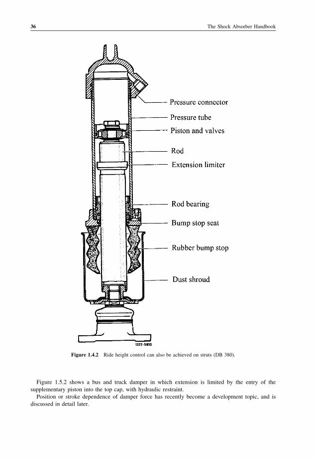
Ordinary passenger cars have so far rarely used dampers with designed position dependence (other
than indirectly, through the effect of the rubber mounting bushes), although they have been widely
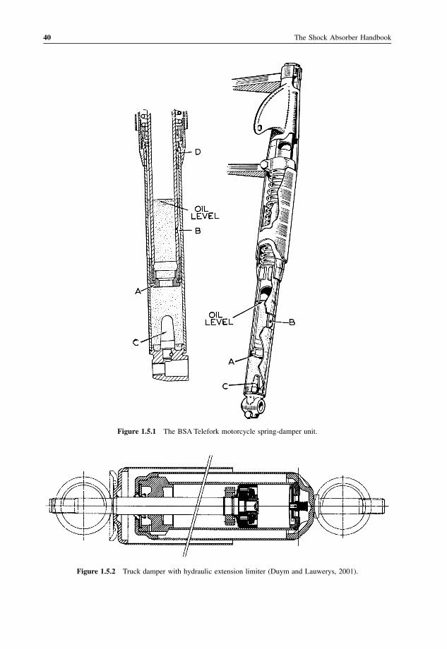
used on motorcycles and aircraft undercarriages. Figure 1.5.1 shows an example motorcycle front
fork in which the sometimes problematic dive under braking is controlled by an internal bump stop
which closes an orifice. This greatly softens the impact and allows weaker springing with improved
ride quality. This basic method of position dependence by the sliding of a tapered needle in a hole
to vary an orifice area has been used for aircraft undercarriages. In the Telefork the further feature
is added that the rather short and blunt rubber ‘needle’ C entering orifice A can distort under
pressure.
Figure 1.3.29 Electromagnetic damper configuration (after Suda et al., 2004).
Figure 1.4.1 With an upper gas chamber, as in most dampers, the provision of a pump, a control system and a few
pipes allows ride height compensation at modest cost (Delco).
Introduction 35
Page 54
Figure 1.5.2 shows a bus and truck damper in which extension is limited by the entry of the
supplementary piston into the top cap, with hydraulic restraint.
Position or stroke dependence of damper force has recently become a development topic, and is
discussed in detail later.
Figure 1.4.2 Ride height control can also be achieved on struts (DB 380).
36 The Shock Absorber Handbook
Page 55
1.6 General Form of the Telescopic Damper
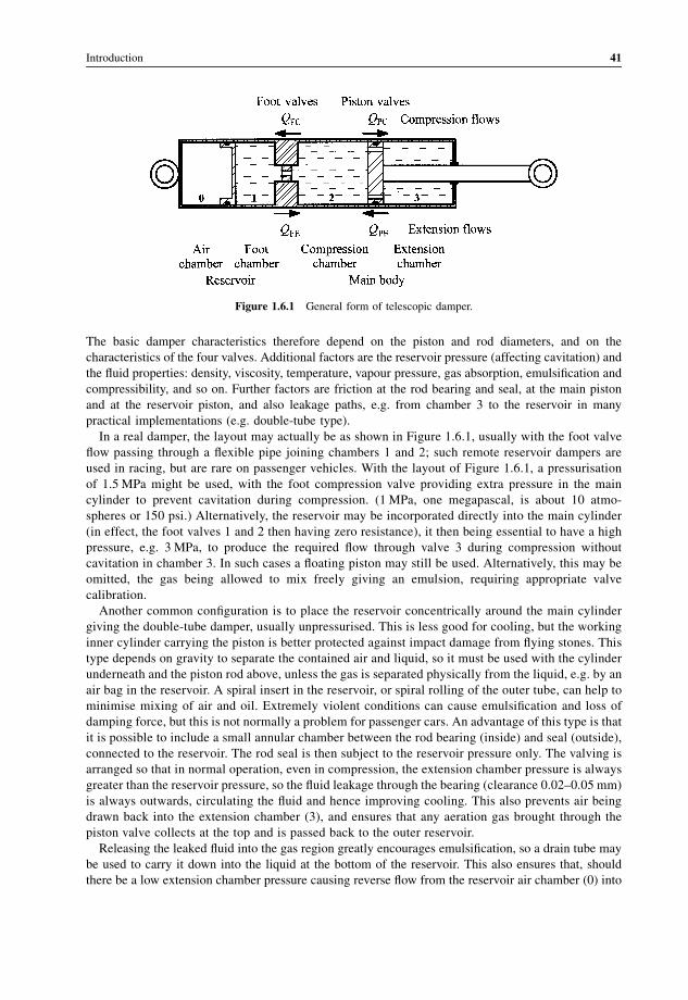
A general form of the telescopic damper is shown in Figure 1.6.1, where there is a separate
reservoir (chambers 0 and 1). Chamber 0 contains air, possibly pressurised, separated by a floating
piston from chamber 1. Chamber 2 is called the compression chamber, at high pressure during
compression, and chamber 3 is called the extension, expansion or rebound chamber, at high
pressure during extension. During compression, fluid is displaced from the main cylinder (chamber
2 and 3) into the reservoir, through a restriction of given characteristics, the compression foot valve.
By the Principle of Fluid Continuity, in normal noncavitating operation, neglecting compressibility,
the quantity of fluid displaced through the foot valve is equal to the volume of the piston rod
entering the main cylinder. During compression, fluid also passes through the piston from chamber
2 to chamber 3, through the piston compression valve. During damper extension, removal of the
piston rod from the main cylinder requires a flow from the reservoir into the main cylinder, through
the foot extension valve. Also, fluid passes through the piston extension valve, valve 4, from
chamber 3 to chamber 2.
Figure 1.4.3 Boge Hydromat (left) and Nivomat (right) height-adjusting dampers.
Introduction 37
Page 56
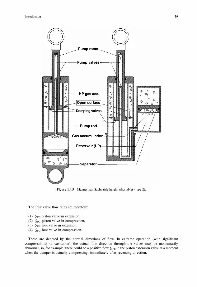
Figure 1.4.4 Mannesman Sachs height adjusting (type 1).
38 The Shock Absorber Handbook
Page 57
The four valve flow rates are therefore:
(1) QPE piston valve in extension,
(2) QPC piston valve in compression,
(3) QFE foot valve in extension,
(4) QFC foot valve in compression.
These are denoted by the normal directions of flow. In extreme operation (with significant
compressibility or cavitation), the actual flow direction through the valves may be momentarily
abnormal, so, for example, there could be a positive flow QPE in the piston extension valve at a moment
when the damper is actually compressing, immediately after reversing direction.
Figure 1.4.5 Mannesman Sachs ride-height adjustables (type 2).
Introduction 39
Page 58
Figure 1.5.1 The BSA Telefork motorcycle spring-damper unit.
Figure 1.5.2 Truck damper with hydraulic extension limiter (Duym and Lauwerys, 2001).
40 The Shock Absorber Handbook
Page 59
The basic damper characteristics therefore depend on the piston and rod diameters, and on the
characteristics of the four valves. Additional factors are the reservoir pressure (affecting cavitation) and
the fluid properties: density, viscosity, temperature, vapour pressure, gas absorption, emulsification and
compressibility, and so on. Further factors are friction at the rod bearing and seal, at the main piston
and at the reservoir piston, and also leakage paths, e.g. from chamber 3 to the reservoir in many
practical implementations (e.g. double-tube type).
In a real damper, the layout may actually be as shown in Figure 1.6.1, usually with the foot valve
flow passing through a flexible pipe joining chambers 1 and 2; such remote reservoir dampers are
used in racing, but are rare on passenger vehicles. With the layout of Figure 1.6.1, a pressurisation
of 1.5 MPa might be used, with the foot compression valve providing extra pressure in the main
cylinder to prevent cavitation during compression. (1 MPa, one megapascal, is about 10 atmo-
spheres or 150 psi.) Alternatively, the reservoir may be incorporated directly into the main cylinder
(in effect, the foot valves 1 and 2 then having zero resistance), it then being essential to have a high
pressure, e.g. 3 MPa, to produce the required flow through valve 3 during compression without
cavitation in chamber 3. In such cases a floating piston may still be used. Alternatively, this may be
omitted, the gas being allowed to mix freely giving an emulsion, requiring appropriate valve
calibration.
Another common configuration is to place the reservoir concentrically around the main cylinder
giving the double-tube damper, usually unpressurised. This is less good for cooling, but the working
inner cylinder carrying the piston is better protected against impact damage from flying stones. This
type depends on gravity to separate the contained air and liquid, so it must be used with the cylinder
underneath and the piston rod above, unless the gas is separated physically from the liquid, e.g. by an
air bag in the reservoir. A spiral insert in the reservoir, or spiral rolling of the outer tube, can help to
minimise mixing of air and oil. Extremely violent conditions can cause emulsification and loss of
damping force, but this is not normally a problem for passenger cars. An advantage of this type is that
it is possible to include a small annular chamber between the rod bearing (inside) and seal (outside),
connected to the reservoir. The rod seal is then subject to the reservoir pressure only. The valving is
arranged so that in normal operation, even in compression, the extension chamber pressure is always
greater than the reservoir pressure, so the fluid leakage through the bearing (clearance 0.02–0.05 mm)
is always outwards, circulating the fluid and hence improving cooling. This also prevents air being
drawn back into the extension chamber (3), and ensures that any aeration gas brought through the
piston valve collects at the top and is passed back to the outer reservoir.
Releasing the leaked fluid into the gas region greatly encourages emulsification, so a drain tube may
be used to carry it down into the liquid at the bottom of the reservoir. This also ensures that, should
there be a low extension chamber pressure causing reverse flow from the reservoir air chamber (0) into
Figure 1.6.1 General form of telescopic damper.
Introduction 41
Page 60
the extension chamber (3), liquid rather than air is drawn back in. Otherwise, gas can pass very rapidly
through the bearing bush, much more rapidly than liquid, with subsequent loss of damping function.
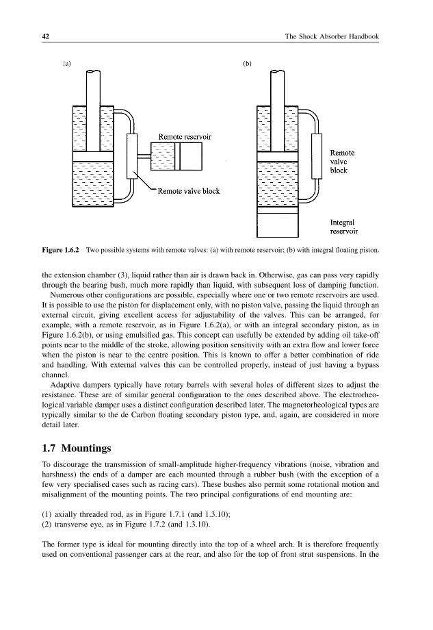
Numerous other configurations are possible, especially where one or two remote reservoirs are used.
It is possible to use the piston for displacement only, with no piston valve, passing the liquid through an
external circuit, giving excellent access for adjustability of the valves. This can be arranged, for
example, with a remote reservoir, as in Figure 1.6.2(a), or with an integral secondary piston, as in
Figure 1.6.2(b), or using emulsified gas. This concept can usefully be extended by adding oil take-off
points near to the middle of the stroke, allowing position sensitivity with an extra flow and lower force
when the piston is near to the centre position. This is known to offer a better combination of ride
and handling. With external valves this can be controlled properly, instead of just having a bypass
channel.
Adaptive dampers typically have rotary barrels with several holes of different sizes to adjust the
resistance. These are of similar general configuration to the ones described above. The electrorheo-
logical variable damper uses a distinct configuration described later. The magnetorheological types are
typically similar to the de Carbon floating secondary piston type, and, again, are considered in more
detail later.
1.7 Mountings
To discourage the transmission of small-amplitude higher-frequency vibrations (noise, vibration and
harshness) the ends of a damper are each mounted through a rubber bush (with the exception of a
few very specialised cases such as racing cars). These bushes also permit some rotational motion and
misalignment of the mounting points. The two principal configurations of end mounting are:
(1) axially threaded rod, as in Figure 1.7.1 (and 1.3.10);
(2) transverse eye, as in Figure 1.7.2 (and 1.3.10).
The former type is ideal for mounting directly into the top of a wheel arch. It is therefore frequently
used on conventional passenger cars at the rear, and also for the top of front strut suspensions. In the
Figure 1.6.2 Two possible systems with remote valves: (a) with remote reservoir; (b) with integral floating piston.
42 The Shock Absorber Handbook
Page 61
latter case, the bottom mounting of the strut is usually a ball joint, forming the lower defining point of
the steering axis. The threaded rod is easily formed by machining the end of the damper rod or by
inserting a stud.
The transverse eye of Figure 1.7.2. uses a concentric rubber bush with a bolt through. Preferably it is
mounted in double shear, but frequently it simply uses a single bolt or stud into the side of the
wheel upright or into the suspension arm. Figures 1.7.3–1.7.5. show some other common types of
mounting.
The effect of the rubber mounting bushes is to put a nonlinear compliance in series with the damper,
giving the complete unit a characteristic which depends upon the displacement amplitude, for a test at a
given velocity amplitude. Small-amplitude motions with high frequencies are more readily met by bush
compliance, hence reducing the transmission of such motions. More substantial movements relating to
deflections of the suspension in handling movements (roll and pitch), or gross suspension movements
in ride at the sprung mass natural frequency, are little affected by the bushes because their small
compliance is effective for only a small deflection. The bushes are therefore important in introducing
some stroke sensitivity to the transmitted forces, keeping the damping high for large amplitudes, as
found in handling motions such as roll in corners, and high for large body motions on rough roads, but
desirably reducing the damping at small amplitudes to improve the ride on smooth roads.
Figure 1.7.1 Axially threaded rod mounting (Reproduced from Kinchin and Stock (1951) pp. 67–86 with
permission).
Figure 1.7.2 Transverse eye or integral sleeve mounting (Reproduced from Kinchin and Stock (1951) pp. 67–86
with permission).
Introduction 43
Page 62
The axial-rod mounting lends itself to an axially asymmetrical form of compliance bushing, as in
Figure 1.7.6 and 1.7.7. The asymmetry may be achieved by differing thickness, area or material
properties, and differing axial preload distance. With a deflection such that one of the two bushes has
expanded to reach axial freedom, that bush then contributes zero further stiffness. If the preload is
small, the essential result is that the stiffness is different for damper compression and extension, a
feature that can be turned to advantage, particularly on strut suspensions.
The basic damper characteristics are normally considered to be those when the mountings are rigid,
not soft bushed, and that is how they are normally tested.
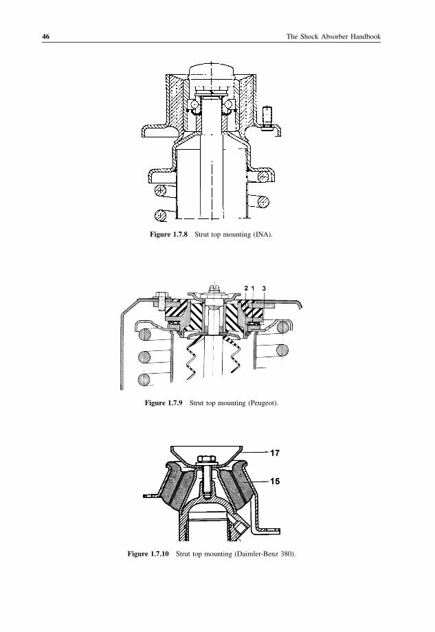
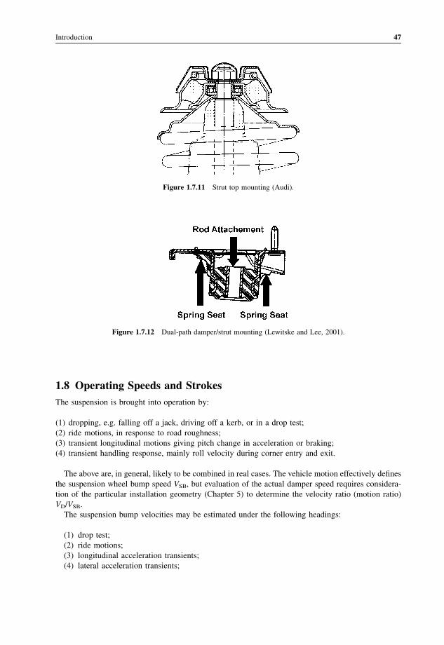
Struts require a more robust mounting than dampers alone, as shown by the examples in Figure 1.7.8
et seq. For front struts there must also be provision for steering action at this point.
It is advantageous to separate the seat force exerted by the spring and the damper. This is natural
in many suspension designs, but not always automatic. Figure 1.7.9 above shows how the separation
may be achieved. This is known as a ‘dual-path mounting’. Figure 1.7.12 gives a further example.
Figure 1.7.3 Integral bar mount (Jackson, 1959).
Figure 1.7.4 Integral stud mount (Jackson, 1959).
44 The Shock Absorber Handbook
Page 63
Figure 1.7.5 Integral bayonet stud mount (Jackson, 1959).
Figure 1.7.6 Asymmetrical type of damper or strut bushing.
Figure 1.7.7 Asymmetrical damper bushing (Puydak and Auda, 1966).
Introduction 45
Page 64
Figure 1.7.8 Strut top mounting (INA).
Figure 1.7.9 Strut top mounting (Peugeot).
Figure 1.7.10 Strut top mounting (Daimler-Benz 380).
46 The Shock Absorber Handbook
Page 65
1.8 Operating Speeds and Strokes
The suspension is brought into operation by:
(1) dropping, e.g. falling off a jack, driving off a kerb, or in a drop test;
(2) ride motions, in response to road roughness;
(3) transient longitudinal motions giving pitch change in acceleration or braking;
(4) transient handling response, mainly roll velocity during corner entry and exit.
The above are, in general, likely to be combined in real cases. The vehicle motion effectively defines
the suspension wheel bump speed VSB, but evaluation of the actual damper speed requires considera-
tion of the particular installation geometry (Chapter 5) to determine the velocity ratio (motion ratio)
VD/VSB.
The suspension bump velocities may be estimated under the following headings:
(1) drop test;
(2) ride motions;
(3) longitudinal acceleration transients;
(4) lateral acceleration transients;
Figure 1.7.11 Strut top mounting (Audi).
Figure 1.7.12 Dual-path damper/strut mounting (Lewitske and Lee, 2001).
Introduction 47
Page 66
(5) combined effects;
(6) damper failure speeds.
These will be dealt with in more detail as follows.
Drop Test
The vehicle is released to fall freely from height hD above the position at which the wheels touch the
ground. The wheels may initially be in the full droop position, simulating the situation where the
vehicle leaves the ground, e.g. a rally car passing over a crest. Where it is intended to simulate a simple
road step-up impact it is better to restrain the wheels to the normal ride position. When the vehicle is
below that point at which contact of wheel and ground just occurs, the springs and dampers will act,
and there will be relatively little further speed increase, unless the drop is from a very low initial
position. This can be studied more accurately, either analytically or by time stepping, but for a simple
high-drop analysis the impact speed VI is given by energy analysis of the fall as
12mV2
I ¼ mghD
where m is the mass and g is the gravitational field strength, leading to
VI ¼ffiffiffiffiffiffiffiffiffiffi
2ghD
p
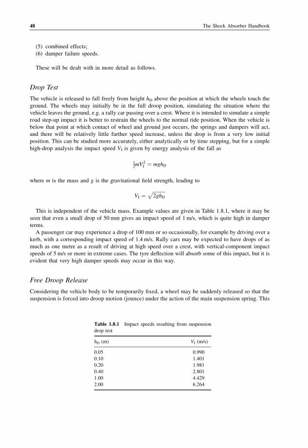
This is independent of the vehicle mass. Example values are given in Table 1.8.1, where it may be
seen that even a small drop of 50 mm gives an impact speed of 1 m/s, which is quite high in damper
terms.
A passenger car may experience a drop of 100 mm or so occasionally, for example by driving over a
kerb, with a corresponding impact speed of 1.4 m/s. Rally cars may be expected to have drops of as
much as one metre as a result of driving at high speed over a crest, with vertical-component impact
speeds of 5 m/s or more in extreme cases. The tyre deflection will absorb some of this impact, but it is
evident that very high damper speeds may occur in this way.
Free Droop Release
Considering the vehicle body to be temporarily fixed, a wheel may be suddenly released so that the
suspension is forced into droop motion (jounce) under the action of the main suspension spring. This
Table 1.8.1 Impact speeds resulting from suspension
drop test
hD (m) VI (m/s)
0.05 0.990
0.10 1.401
0.20 1.981
0.40 2.801
1.00 4.429
2.00 6.264
48 The Shock Absorber Handbook
Page 67
could occur in practical use if one wheel suddenly passes over a wide hole. If the suspension was
previously in a normal position, the free force on the wheel equals the normal suspension force,
about mg/4. This will give a free extension velocity of 2 m/s or more, large in damper terms.
This is the speed at which the car would settle on its dampers if the springs could be instantly
removed:
VR ¼mgP
CD
¼ g
2z
ffiffiffiffiffiffiffiffiffiffi
mP
K
r
¼ g
2zvNH
where the spring stiffnesses K and the damping coefficients CD are the effective values at the wheels.
The natural heave frequency in rad/s is vNH.
In principle this is a feasible experiment, by removing the springs and holding the body, followed by
a sudden release. If the wheel is in a compressed position at the moment of release then the potential
speed is even greater. In practical conditions, of course, the wheel inertia plays a part.
Ride Motions
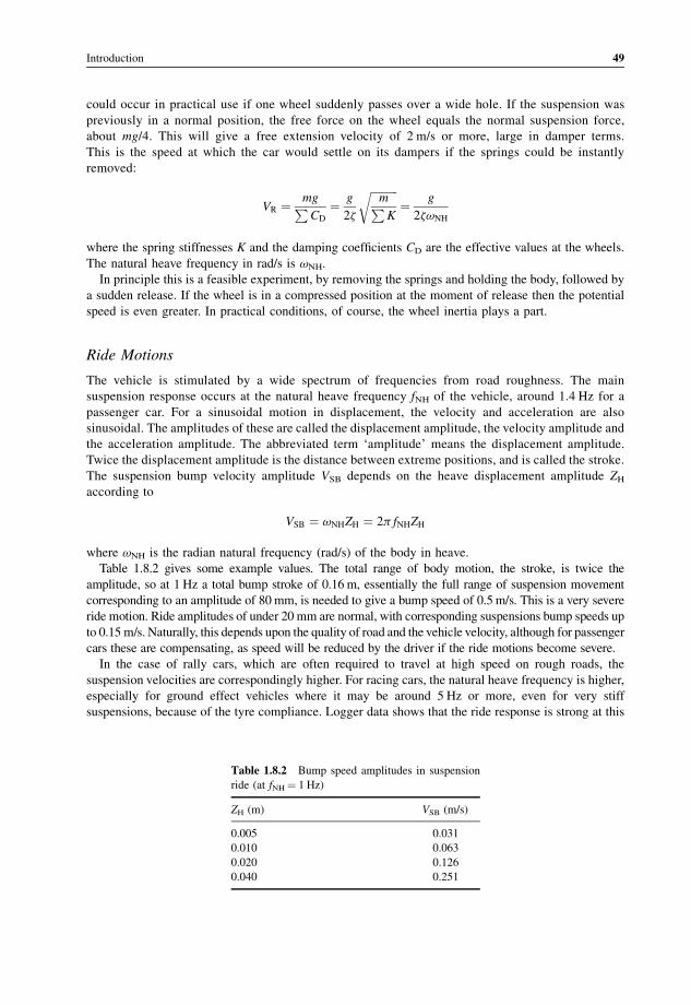
The vehicle is stimulated by a wide spectrum of frequencies from road roughness. The main
suspension response occurs at the natural heave frequency fNH of the vehicle, around 1.4 Hz for a
passenger car. For a sinusoidal motion in displacement, the velocity and acceleration are also
sinusoidal. The amplitudes of these are called the displacement amplitude, the velocity amplitude and
the acceleration amplitude. The abbreviated term ‘amplitude’ means the displacement amplitude.
Twice the displacement amplitude is the distance between extreme positions, and is called the stroke.
The suspension bump velocity amplitude VSB depends on the heave displacement amplitude ZH
according to
VSB ¼ vNHZH ¼ 2p fNHZH
where vNH is the radian natural frequency (rad/s) of the body in heave.
Table 1.8.2 gives some example values. The total range of body motion, the stroke, is twice the
amplitude, so at 1 Hz a total bump stroke of 0.16 m, essentially the full range of suspension movement
corresponding to an amplitude of 80 mm, is needed to give a bump speed of 0.5 m/s. This is a very severe
ride motion. Ride amplitudes of under 20 mm are normal, with corresponding suspensions bump speeds up
to 0.15 m/s. Naturally, this depends upon the quality of road and the vehicle velocity, although for passenger
cars these are compensating, as speed will be reduced by the driver if the ride motions become severe.
In the case of rally cars, which are often required to travel at high speed on rough roads, the
suspension velocities are correspondingly higher. For racing cars, the natural heave frequency is higher,
especially for ground effect vehicles where it may be around 5 Hz or more, even for very stiff
suspensions, because of the tyre compliance. Logger data shows that the ride response is strong at this
Table 1.8.2 Bump speed amplitudes in suspension
ride (at fNH¼ 1 Hz)
ZH (m) VSB (m/s)
0.005 0.031
0.010 0.063
0.020 0.126
0.040 0.251
Introduction 49
Page 68
natural frequency, but the amplitude is necessarily very small, so the actual suspension ride velocities
are still quite modest, generally 0.1–0.2 m/s, although worse over particular bumps.
Longitudinal Acceleration Transients
Variations of longitudinal acceleration cause (angular) pitch motions, and occur by sudden application
or removal of engine power or brake action, with a step change of AX. This is most easily demonstrated
when the brakes are kept firmly on as the vehicle actually comes to a halt, giving a distinct jerk with a
subsequent damped pitching motion. The avoidance of this discomfort factor by ramping off the
braking force at the end is called ‘feathering’ the brakes. This case is a fairly easy one to analyse.
Consider a longitudinal deceleration AX on a simple vehicle having wheelbase L with centre of mass at
the mid point, centre of mass height HG, and suspension stiffness wheel rate KW at each wheel. An
angular pitch angle u radians gives a suspension bump displacement
zSB ¼ 12
Lu
Hence, the restoring pitch moment MP is
MP ¼ 2KWzSBL ¼ KWL2u
and the pitch angular stiffness KP is
KP ¼ KWL2
A longitudinal acceleration AX gives a longitudinal load transfer moment
MAX ¼ mAXHG
with an associated pitch angle
u ¼ MAx
KP
¼ mHG
KWL2AX
and a suspension deflection
zS ¼1
2Lu ¼ mHG
2KWLAX
The natural frequency fNP of pitch motion depends upon the pitch stiffness and also on the sprung
mass (body) second moment of mass in pitch, IPB :
fNP ¼1
2p
ffiffiffiffiffiffi
KP
IPB
r
with a value for most vehicles approximately equal to the heave frequency, at around 1 Hz for a passenger
car. Hence the estimated suspension bump velocity for this amplitude and frequency VSB,Ax is
VSB;Ax ¼ vNPzSB
¼ 2p fNP
mHG
2KWL
� �
AX
50 The Shock Absorber Handbook
Page 69
where vNP is the natural frequency of the body in pitch and zSB is the displacement of the suspension in
bump.
Realistic physical values for a passenger car give a pitch angular deflection of about 0.4�/m s�2(4�/g)
with a suspension deflection/acceleration rate of 10 mm/m s�2 (100 mm/g). At a pitch natural
frequency of 1 Hz the consequent suspension velocity is about 50 mm s�1/m s�2 (0.5 m s�1/g).
Hence the associated suspension velocity for pitch motions is typically up to 0.2 m/s for normal braking
transients and up to 0.5 m/s for extremes. The most severe case is a sudden switch from acceleration to
braking. For a 5 m/s2 (0.5g) change of AX, the suspension stroke is about 50 mm with a velocity of
0.25 m/s.
A similar analysis may be performed for other kinds of vehicle. Racing cars, despite their high
natural pitch and heave frequencies, tend to have smaller suspension travel velocities because of the
limited suspension movements, plus the use of anti-dive suspension geometry, which reduces the pitch
angles and velocities in proportion.
Lateral Transients (roll)
Sudden changes of lateral acceleration cause roll motions that can be analysed in a similar way to
longitudinal motions. A lateral acceleration causes a suspension roll angle
fS ¼ k’SAy
where k’s is the suspension roll angle gradient, of about 0.014 rad/m s�2 (0.80 �/m s�2, 8�/g,
0.14 rad/g). The corresponding suspension deflection zS is
zS ¼ 12f ST
with fS in radians and a track (tread) T of about 1.5 m. For a roll natural frequency fNR the suspension
velocity amplitude estimate becomes
VSB;Ay ¼ 2p fNRzSB ¼ p fNRfST
Realistic values for a passenger car are a natural roll frequency of 1.5 Hz and a suspension deflection
of 10 mm/m s�2 (100 mm/g). Entering a normal corner of lateral acceleration 3 m/s2 (0.3g), the
suspension deflection is about 30 mm and velocity 0.30 m/s. An extreme corner entry gives 80 mm
stroke and 0.60 m/s, depending on the time for steering wheel movement.
It is essential to have good roll damping in this speed range. This is the basic reason why nonlinear
F(V) characteristics are used—to give adequate roll damping without excess forces at higher speed.
Combinations
The above suspension velocities are frequently combined. In general a handling motion is mixed with
some ride motion, so the handling motion does not always occur in a progressive manner, there may
even be velocity reversals.
Overall, for a passenger car the suspension bump velocities are up to 0.3 m/s in normal driving, up to
1 m/s in harder driving or poorer roads, with values in the range 1 to 2 m/s occurring relatively rarely.
Table 1.8.3 indicates a possible classification of bump velocity ranges for passenger cars. A racing
car classification would generally be lower, especially for a ground effect vehicle such as Formula 1, or
Indy. However, even ground effect racing cars are subject to driving over angled kerbs, to dropping
from jacks and so on.
Introduction 51
Page 70
Damper Failure Speeds
The damper will suffer permanent damage if subject to excessive velocities, although these limits are
not widely advertised. The physical survival limit speed is that which will not quite cause any metal
yielding or, more likely first, damage to the valves or seals. The limit speed is typically around 5 m/s.
Velocity and Stroke
Fukushima et al. (1983) suggested that dampers should have a stroke-dependent characteristic, such that
for a given velocity a longer stroke would give a greater force. More information on this is given in
Chapter 3. Table 1.8.4 shows the velocities and strokes found by Fukushima, with some extra analysis,
where F/V is the desirable CD, and F/S is the desirable ‘stiffness’ relationship if the force were produced
by a spring. Slow steering is a ‘figure of 8’ course with large lateral acceleration, but gentle entry.
Perhaps the clearest form of analysis for this problem is to plot a diagram of damper velocity against
amplitude or stroke, showing the active points. This is done in Figure 1.8.1. Points on one line radiating
from the origin have the same frequency, since the velocity and displacement amplitudes of a
sinusoidal motion are related by V ¼ 2pfX. With suitable scales for a particular vehicle, the main
diagonal is the natural frequency of the vehicle body in heave type motions, around 1.4 Hz. The basic
handling manoeuvres, i.e. changes of AX and AY, operate along this diagonal according to severity, or
somewhat below it, according to the rate of application of the controls. Driving along a straight road
gives heave motions along the main diagonal, with good-quality roads at the bottom left, and rough
roads, or fast driving, further up. Bumps act on the bottom of the wheel and are transmitted through to
the body at essentially the wheel hop frequency. Isolated bumps therefore lie on a steep line at about
12 Hz, on the left.
To avoid transmission of bumps, but to give good damping for handling evidently could be achieved
by having frequency-dependent damping, within the meaning of this diagram, with low damping
Table 1.8.3 Possible classification of suspension bump velocities (m/s)
Passenger car Racing car (F1, Indy)
Very low Below 0.1 Below 0.025
Low 0.1 – 0.2 0.025 – 0.050
Medium 0.2 – 0.4 0.050 – 0.080
High 0.4 – 1.0 0.080 – 0.200
Very high 1.0 – 2.0 0.200 – 0.400
Extreme Above 2.0 Above 0.400
Table 1.8.4 Suspension stroke, velocity and damper force
Manoeuvre Stroke (mm) V (m/s) F (N) F/V (kN s/m) F/S (kN/m)
Slow steering 50 0.02 48 2.4 1.0
Rapid steering 45 0.12 288 2.4 6.4
Lane change 25 0.06 144 2.4 5.8
Single bumps 4 0.40 120 0.3 30.0
Brake/accelerate 50 0.20 400 2.0 8.0
Smooth road 3 0.08 8 0.1 2.7
Rough road 12 0.60 600 1.0 50.0
(Based on Fukushima et al., 1983)
52 The Shock Absorber Handbook
Page 71
above, say, 3 Hz. On the other hand, to also have low damping as desired on smooth roads, stroke-
dependent damping with low damping for strokes below about 10 mm is desirable.
1.9 Manufacture
The complete manufacturing process involves:
(1) material production;
(2) individual component production;
(3) assembly;
(4) oil-filling;
(5) pressurisation (in some cases);
(6) insertion of bushes;
(7) external finishing;
(8) testing at various stages as appropriate.
Initial material production is of course not the province of the damper manufacturer, who will simply
buy in materials, but may heat-treat them.
The production method of the tubes depends upon the price range of the damper. Cheaper ones may
have tubes rolled from low-carbon steel with a resistance-welded seam. More expensive ones may
avoid the seam by using extruded tubing, and in any case racing dampers, and possibly more passenger
cars in the future, will have aluminium cylinders to reduce the weight. Steel tubes are annealed and
then cold-drawn to final diameter, giving accurate sizing and cold-worked strength. The internal finish
is important to give a good seal with the piston and also to give a low wear rate of the piston seal; the
internal finishing process, e.g. honing, varies with manufacturer and budget.
Figure 1.8.1 Damper speed versus damper amplitude for various ride and handling activities. Handling
‘frequency’ depends on the rate of control application.
Introduction 53
Page 72
The piston rod is normally made from high-carbon steel with cold-forged ends, often with some
drilled passages, possibly threaded at the top, and case-hardened or chromed on rubbing areas. The life
of the rod-bush bearing and of the main rod seal is sensitive to the rod surface finish, which should be
0.1 mm r.m.s. or better, achieved by grinding and lapping. It is now normal to use a hard-chrome-plated
rod which enhances both wear resistance and corrosion resistance.
Pistons themselves may be forged or sintered. Piston seals vary considerably. Some have iron piston
rings not unlike those in an engine, with a small end gap, necessary for thermal expansion. Plastic
piston-type rings are also used, typically with stepped-overlapped ends, from Teflon (PTFE) or nylon,
etc. Similar designs are used in Tufnol and other paper and cloth-reinforced phenolic materials. Square-
section rubber rings and O-ring seals are common. Finally, some plastic seals are moulded solid to the
piston with no apparent attempt to allow for self-adjustment to fit, possibly expected to run-in to a
minimal correct working clearance, with a wide contact area. Racing pistons are usually machined
aluminium, turned and drilled, with a plastic piston ring
Valve manufacture of course varies with design. At the low-cost high-volume end of the market,
where possible, stamping and pressing are used, followed by automated or manual assembly of these
parts plus coil springs, washers, et cetera.
For common double-tube dampers, the top and bottom cylinder ends are pressed from steel sheet,
typically with a mounting bush ring spot-welded onto the bottom one. The lower cup is welded to the
cylinder and foot valve inserted. The piston, piston valves, rod, rod-bush housing, top cup and its seal
and bearing are assembled. The piston and oil are inserted and the top cup welded, spun or crimped into
place. The rubber bushes are then pressed in, and, finally, paint is applied.
With a worldwide production of several hundred million dampers per year, there is obviously a
considerable difference between the methods used for price-sensitive mass-production units and those
for higher-price small-volume precision units produced for specialised applications such as racing and
rallying.
1.10 Literature Review
Books on vehicle suspension or vehicle dynamics nearly always have some basic description of damper
(shock absorber) design and operating characteristics, although this is invariably limited in scope e.g.:
(1) Norbye (1980), 10 pages descriptive;
(2) Campbell (1981), 8 pages descriptive, one equation;
(3) Bastow (1987), 10 pages on the effect of damping, 19 pages of description of dampers;
(4) Dixon (1991, 1996), 10 pages on history plus comments on effect on handling;
(5) Gillespie (1992), 7 pages on dampers and their effect;
(6) Milliken and Milliken (1995), 50 pages, almost all on vehicle behaviour rather than damper design
itself;
(7) Haney and Braun (1995), 32 pages, with the emphasis on racing car dampers;
(8) Reimpell and Stoll (1996), 36 pages, on damper design, construction and characteristics.
Within the context of a complete book on ride, or on handling, or on vehicle dynamics as a whole,
such limited treatment is understandable.
Although a literature search reveals several thousand papers referring to ‘damper’ or ‘shock
absorber’ in the context of vehicles, rather few of these are about the design and characteristics of
the damper itself. A full list of these is given in the references.
The earliest paper appears to be that by Hadley (1928), which deals with mechanical friction
dampers, seeking to obtain a suitable characteristic by position dependence. The ability of a damper to
control large amplitudes adequately whilst not overdamping small motions is called the ‘range’ of the
54 The Shock Absorber Handbook
Page 73
damper, and was a leading problem of that era. It seems surprising now that mechanical types were
considered more promising than hydraulics.
Weaver (1929) investigated damper characteristics by applying them to a vibrating system, actually a
272 kg mass on a 31 kN/m spring giving 1.71 Hz undamped natural frequency, with initial deflections
of typically 76 mm, and producing free vibration F(X) plots, which are roughly spiral for less than
critical damping. This is a simple and cheap method of investigation, of some value for comparative
purposes, but not as useful as an F(X) curve for a controlled displacement pattern, preferably
sinusoidal, as obtained on a modern testing machine.
Nickelsen (1930) states that by 1930 nearly all cars had some kind of damper as standard equipment,
and therefore, of course, by implication some still did not. He concentrates on the double-acting
hydraulic type, recommending that no more than 20% of the resistance should be in bump. F(X) curves
are shown, and temperature fade considered, although with the apparent belief that resistance is simply
proportional to viscosity.
James and Ullery (1932) discuss the problems of Coulomb friction against the advantages of
hydraulic damping with a suitable force–speed relationship. Various force–displacement graphs (‘card
diagrams’) are shown, illustrating various effects and faults, and the loss of damping effect with
temperature rise is eliminated by a variable orifice comprising a plug valve regulated by a bimetallic
strip. Oil viscosities of 20–200 centistokes were in use. They emphasise the need for a smooth
characteristic, building up with speed, and the need for temperature compensation.
Fuchs (1933) gives F(X) diagrams for single-acting and double-acting hydraulics, and for the old
friction disc type, and also shows a characteristic in the phase plane (V–X) for a position–dependent and
force–dependent damper.
Kindl (1933) proposed to regulate the damper by a valve controlled by body inertia, so that wheel-
only movements are free, but the body motion is damped. Unfortunately his acceleration sensor and
controller was a 680 g mass for each damper. However, with electrically controlled dampers, and
modern sensors and control systems, this is an idea whose time may now be ripe.
Schilling and Fuchs (1941) show force–speed diagrams for year 1940 passenger car dampers,
some of which are similar to modern dampers, showing a predominance of rebound force over
bump.
Connor (1946) distinguishes various types of damping effect (Coulomb, real dry friction, viscous,
degenerate viscous, ‘hydraulic’ damping proportional to V2, and solid material hysteresis). Typical
damping ratios are stated to be 0.15–0.20, and the temperature rise in a telescopic damper is stated to
be about 50�C on extremely rough roads, although only about 20�C for rotary and cam types because of
conductivity into the vehicle body.
The related area of buffer design is considered by Brown (1948), Tatarinov (1948, 1949) and
Brown (1950 a, b). For buffering, the resisting force is commonly made a function of position. This
is not normally done for car dampers, although it has been used on motorcycle front forks, where it
gives a bump stop effect, but is regarded as superior to an elastic bump stop because of reduced
spring back.
Kinchin and Stock (1951/1952), in a comprehensive paper, discuss various details, such as the
physical layout of various hydraulic types, fluids, testing, operating problems such as aeration,
fade, noise problems, flow resistances, and force–displacement F(X) diagram (work diagram)
shapes.
Peterson (1953) describes the introduction of a damper designed to have a linear characteristic
(in contrast to many of the previous ones which were almost Coulomb in character, as may also
be seen in some of the characteristics shown by Schilling and Fuchs (1941). Prototypes had tubes
intended to give a simple viscous pressure drop, but actually giving force proportional to speed
to the power 1.25. More conventional drilled and coined holes were used for production.
The higher forces obtained at high speeds were considered a substantial improvement for rough
roads.
Introduction 55
Page 74
Cline (1958) discusses various aspects of dampers in general terms, giving some example F(X)
curves, with brief comments on the effect of valve changes. He also shows a photograph of the then
new Gabriel dampers with electrical remote adjustment.
Hoffman (1958) was amongst the first to do analytical work on the damper. He shows various
experimental F(V) and F(X) curves for different types of damper, and used an analogue computer to
study vehicle ride for various dampers.
Jackson (1959) discusses the basic principles of telescopic dampers and their manufacture, and the
effect of valving, stating that control of unsprung mass vibrations had become the greater problem once
independent suspension was introduced. The standard fluid is stated to be straight mineral oil with
viscosity somewhat less than SAE 5, but this was considered unsatisfactory because of viscosity
change with temperature causing difficulties at very low temperatures. High-viscosity-index oils were
just coming into use. Curves of damping force against temperature are given. A freon–filled nylon cell
for preventing aeration problems is described.
Eberan-Eberhorst and Willich (1962) show experimental F(X) curves for various strokes, and F(X)
and F(V) curves with lag and hysteresis. The experimentally observed temperature effect on force was
about �0.1%/K for compression and �0.3%/K for extension. A Plexiglas damper was built, allowing
cavitation to be observed directly.
Ellis and Karbowniczek (1962) deal mainly with buffers rather than vehicle dampers. However, they
draw attention to possibilities for separation of the air from the fluid to prevent aeration, including a
spring-loaded free piston, a diaphragm, a gas-filled bladder, or a compressible closed-cell solid foam.
Speckhart and Harrison (1968) return to the idea by Kindl (1933) of using an inertia-regulated valve,
this time much lighter and built into the damper piston, the intention being to reduce vehicle ride jerk
(rate of change of acceleration).
Polak and Burton (1971) discuss damper construction in general terms, giving attention to possible
designs of amplitude sensitive dampers, to a multi-frequency ‘seismically’ actuated damper (mounted
on the wheel only, not to the body), and propose a configuration with a conventional damper coupled
between suspension and engine. They also mention the possibility of achieving adjustable damping by
the use of certain electrostatically sensitive solid/oil mixtures which have variable viscosity, i.e. use of
electrorheological liquids.
Wossner and Dantele (1971) compare the pressurised single-tube type (with and without a free
separator piston) with the unpressurised dual-tube type, and give experimental results on the cooling
effect of airstreams.
Mitschke and Riesenberg (1972) discuss damper temperature rise on various types of road, and the
consequences for fluid viscosity and damper force.
Mayne (1973) gives an analysis of the effect of liquid and mechanical compliance on buffer
performance.
Jennings (1974) gives 21 F(X) loops for commercially available motorcycle front forks and rear
dampers, which prove to be characterised by extreme compression/extension asymmetry.
Cline (1974) gives a simple review of the application of hydraulic dampers to recreational vehicles,
considering briefly how to achieve some of the particular characteristics required.
Schubert and Racca (1974) describe an unconventional ‘elastomeric-pneumatic isolator with orifice-
type relaxation damping’, proposing application to motor vehicles.
Simanaitis (1976) gives a brief history and a discussion of some of the operating principles and
problems (‘The Dutch call them schokdempers; the French, amortisseurs; and the English, dampers.
Indeed, many early automotive designers called them unnecessary . . .’). (As a matter of interest it is
Stossdampfer in German and ammortizzatori in Italian.) Oil viscosities are given as SAE 5 to 10.
Aeration is stated to be the cause of compression lag (although actually this can also be cavitation or
desorption of air). Manufacturing methods are outlined.
Dalibert (1977) considers the effect of some oil properties on damper performance. The sensitivity of
peak force to temperature was found to be about �0.3 %/�C, giving a reduction of 35% at 130�C,
56 The Shock Absorber Handbook
Page 75
which is stated to be the approximate maximum temperature encountered with hard driving on bad
roads. Maximum safe viscosity is stated to be 4000 cs at the lowest temperature, and a minimum of 4 to
7 cs at 100 �C, depending on design. Noise problems are considered in some detail.
Segel and Lang (1981) report a detailed investigation (additional information being given in Lang’s PhD
thesis (1977), using an 82 parameter analogue computer model that gave quite good agreement with the
experimental data obtained. Compressibility of the liquid, plus a slight additional effect from cylinder
compliance, was found to give hysteresis in the F(V) curve at higher frequencies (above 1 Hz). Presumably
series rubber bushes would markedly increase this effect, but were not mentioned. Gas compressibility and
absorption were considered; this could not readily be handled by the analogue computer, but the use of an
effective vapour pressure of up to 70 kPa (instead of the actual value of less than 2 kPa) was found to give
realistic results. Orifice discharge coefficients were investigated, but for simplicity it was considered that a
constant value of 0.7 was acceptable. Testing was actually done with a square acceleration wave, giving a
triangular speed waveform and a piecewise parabolic displacement waveform.
Van Vliet and Sankar (1981) studied motorcycle forks and rear dampers, using analogue and digital
simulations respectively to obtain good agreement with experimental F(X) diagrams.
Arndt et al. (1981) consider seal design with tests of friction especially in the context of smaller,
lighter vehicles where the problem seems more critical, advocating a lip design with a lubrication
groove, allowing improved ride comfort and reduced pressurisation.
Ohtake et al. (1981) also consider seal design, with tests of friction and durability, and analysis of
relevant parameters, considering variation of optimum design with details of the application.
Fukushima et al. (1983) advocate stroke-sensitive damping, and present the arguments in its favour,
including analysis of ride and handling motions.
Fukushima et al. (1984) reiterate the points on stroke-sensitive damping, and consider a vortex valve
type which has a resistance that depends on stroke as well as speed, being greater for larger stroke.
They made successful tests of a demonstration unit.
Steeples et al. (1984) describe a damper testing facility, with the emphasis on durability testing.
Morman (1984) considers the mathematical modelling of dampers, expressed in terms of governing
differential equations.
Holman (1984) considers a rotary-type damper configured to give better immunity to stone impact
damage, intended for military and off-road vehicles.
Yukimasa et al. (1985) consider the design of oil and gas seals, sealing quality and frictional
characteristics of damper seals.
Vannucci (1985) considers damper noise problems with special reference to the McPherson strut
with integral damper.
Sugasawa et al. (1985) studied theoretically the optimum damping for ride and handling indepen-
dently for a two-degrees-of-freedom system, and tested an automatically adjusting damper system
using sensors for control inputs (accelerator, brakes, steering) and an ultrasonic ride height measure-
ment to appraise the road quality.
Browne and Hamburg (1986) measured damper temperatures, and also the simultaneous forces and
velocities of dampers on the vehicle, to obtain the energy dissipation rates. For passenger cars on
normal roadways this was found to be 3–60 W, and about 12 W on average.
Karadayi and Masada (1986) consider factors such as directional asymmetry, dry friction, hysteresis,
compressibility and backlash in a nonlinear model, aiming to create a simple damper model (i.e. fast
computing) suitable for use in vehicle simulations. The total nonlinear compressibility is treated as
piecewise linear, giving in effect a backlash plus a series stiffness, with Coulomb friction and
asymmetric linear damping. The model gives quite good agreement with the general character of
the real F(V) curves, although the quantitative agreement is not particularly good, which presumably is
the result of, rather oddly, omitting the most important nonlinearity of all, the resistance characteristics
of the fluid valves. The usual end-fitting rubber bushes are not mentioned, but presumably could readily
be incorporated in this model.
Introduction 57
Page 76
Young (1986) gives details of the internal configuration of various types of aircraft undercarriage
dampers, which typically have free-piston gas separation and positional dependence of the damping
force.
Hall and Gill (1986) describe a CSMP digital simulation of a dual-tube damper, including the effect
of valve mass and valve damping. The foot compression valve (compression control) is a side exit
spool valve, giving a fluid momentum force that gives Coulomb friction between the spool and its
guide—another possible source of F(V) curve hysteresis. Gas compressibility is dealt with by adopting
a high effective vapour pressure of 41–85 kPa. In the simulation, a time step not exceeding 10 ms was
necessary to avoid instability, corresponding to 0.02� of phase angle. Leakages and temperature effects
were neglected, and a constant discharge coefficient of 0.7 was used. With an empirically selected
effective vapour pressure, the trend of results was correct, but the F(V) behaviour was too oscillatory,
either because of inadequate theoretical valve damping or inadequate experimental sensor frequency
response.
Soltis (1987) describes the Ford PRC (Programmed Ride Control) automatic damper adjustment
system, particularly considering the handling conditions when high damping is desirable, and the
advantages of the use of steering wheel angle sensing.
Su et al. (1989) theoretically analysed an adaptive damper, concluding that significant improvements
in ride performance could be achieved.
Gvineriya et al. (1989) investigated the extension of gas spring units to include gas suspension
damping, considering it to be a viable option.
Lemme and Furrer (1990) describe a self-powered system for remotely adjusting dampers by
hydraulic means.
Hennecke et al. (1990a, b) describe an in-production adaptive damping system, with three states
independently for each axle according to road conditions and driver. This system uses body sensors for
vertical acceleration above the axles, steering angle, and longitudinal speed and longitudinal accel-
eration (rather than brake line pressure and engine output), with electronic control of solenoid valves.
Hagele et al. (1990) tested variable dampers with fast-acting solenoid valves and electrorheological
liquids, but found the latter as yet unsatisfactory.
Fan and Anderson (1990) tested a bus damper complete with its rubber mounting bushes, naturally
obtaining a large hysteresis in the F(V) curve. Modelling equations are presented, with the bushes
represented as effective compressibility, and good correlation with experiments is shown, with
frequency-dependent hysteresis.
Rakheja et al. (1990) studied a ‘sequential’ damper similar to a conventional positive damper with
multi-stage asymmetrical valving proposed to be mounted externally to facilitate adjustment,
concluding that it offered significant possible improvements in ride over a conventional damper.
Lemme (1990) considers the advantages of hydraulic control for variable dampers over electrical
control, considering in detail the design of such a damper, with the idea that action of any one damper
could produce a pressure to control all four damper settings, without other sensors.
Kumagai et al. (1991) studied the internal Coulomb friction of strut bearings relating to the
transmission of NVH (noise, vibration and harshness).
Patten et al. (1991) described how fast semi-active dampers can take advantage of the
phase relationship between front and rear axle disturbances to give a significant improvement in
ride quality.
Shiozaki et al. (1991) propose a variable damper with piezoelectric sensor and actuator built into the
damper rod, with rapid response (3 ms) and high actuation force for an axial valve, favouring a
‘normally hard’ setting with switching to soft when appropriate, e.g. hitting a bump. The short
piezoelectric actuator motion is amplified by stacking the elements, and then amplifying the total
motion with an inverted hydraulic jack method to give 2 mm of motion at the valve.
Tamura et al. (1992) consider the development of materials for the rod-guide bush of strut type
suspensions, which carries a large side load with unreliable lubrication, but needs to have low friction
58 The Shock Absorber Handbook
Page 77
and long life, and is subject to other problems such as cavitation erosion. Various PTFE/Sn/Pb/Cu/PbF2
sintered materials have been used.
Petek (1992a, b, c) describes the design principles of and tests on an experimental design of variable
damper using ER (electrorheological) liquid, with durability tests and a retrofit vehicle road test. The
ER effect is claimed to be fast in action (time constant about 5 ms), with good control power input
efficiency (about 4 W), and giving lower cost and better reliability than mechanical valves, although the
desired operating temperature range of �40 to þ120 deg C may be a problem.
Nall and Steyn (1994) performed experimental evaluation of various control strategies for two-state
dampers under practical conditions. It was concluded that such dampers offered significant ride
improvements, and that the usual theoretical assessment of adaptive dampers did not adequately
represent real conditions.
Pinkos et al. (1993) espouse ERM (electrorheological-magnetic, i.e. MR magnetorheological)
liquid, which operates at low voltage. This was used in a lever-arm configuration test damper for
road tests.
Baracat (1993) gives a theoretical analysis of damper forces and compares the predictions with
experimental results.
Reybrouck (1994) considers modelling of conventional dampers to allow for force dependencies not
just on velocity, but also on position, acceleration, temperature etc. for application in ride quality
simulations, obtaining good agreement with experimental results.
Fash (1994) studied the application of a neural net computation model to data from dampers
installed on vehicles. Correlation with the forces was superior to that of a simple linear model.
Besinger et al. (1995) describe a seven parameter damper model, particularly developed for use with
studies of heavy vehicles. The model is compared with test damper data, and the effect of variation of
the parameters on vehicle ride is investigated by simulation.
Sturk et al. (1995) developed and tested a high-voltage control unit for an electrorheological variable
damper, and experimentally investigated the effect of control strategies on ride with a quarter-car rig.
Whelan (1995) investigated the use of triangular position waveform testing.
Cafferty et al. (1995) performed damper testing with excitation by a random waveform.
Audenino and Belingardi (1995) considered models of varying complexity for motorcycle dampers
in comparison with experimental data.
Angermann (1995) investigated the use of aluminium bodies for dampers, and other means of weight
reduction for passenger cars, already common on racing cars.
Petek et al. (1995) tested a complete electrorheological system on a vehicle, giving information on
the support systems and control logic, concluding that such systems would be good if the working
temperature range required for general use could be achieved.
La Joie (1996) discusses detailed damper modelling and comparison with experimental results,
concentrating on racing dampers.
Haney (1996) made a bench comparison of several adjustable racing car dampers and presented their
experimentally measured characteristics.
Ryan (1996) considers the merits of remote reservoir dampers with high shaft-displacement forces.
Warner and Rakheja (1996) investigated friction and gas spring characteristics, varying with
temperature, with a particular emphasis on the significance of the latter for critical racing car ride
heights.
Feigel and Romano (1996) describe a directly controlled electromagnetic valve for a damper.
Duym (1997) considers representation of damper characteristics to allow for the presence of
hysteresis effects on the F(V) curve, concluding that velocity and acceleration make a more satisfactory
combination of variables than velocity and position.
Cafferty and Tomlinson (1997) discuss representation of damper characteristics by frequency
domain techniques.
Tavner et al. (1997) consider test procedures for switchable dampers on the vehicle.
Introduction 59
Page 78
Kutsche et al. (1997) discuss pneumatically controlled variable truck dampers.
Lee (1997) analyses the double-acting shim valve monotube damper, using dimensional analysis and
finite element analysis to deal with the nonlinear shim deflections.
Meller (1999) describes self-energising self-levelling systems and their incorporation into hydraulic
dampers.
Herr et al. (1999) used a CFD (computational fluid dynamic) model to study flow in damper valves
and to predict complete damper forces, obtaining good agreement with experimental results.
Els and Holman (1999) drew attention to the advantages of the lever-arm rotary damper in heavy
duty applications.
Lion and Loose (2002) performed a thermomechanical analysis of dampers with experimental tests.
Choi (2003) tested a design of ER damper in which the ER effect was used to control the main valve
rather than providing all the extra resistance itself.
Yamauchi et al. (2003) investigated a noisy strut suspension vibration arising from rod bending
stimulated by damper piston friction against the tube, successfully obtaining a simple design criterion
and testing a double-piston solution giving improved alignment.
Guglielmino and Edge (2004) investigated a dry friction telescopic damper using hydraulic control
of the normal force and hence of the friction, claiming various advantages.
Smith and Wang (2004) investigate the possible application of ‘inerters’ in vehicle suspensions.
Suda et al. (2004) studied the possible use of an electromagnetic damper in telescopic form, with a
high pitch shaft driving a ball nut which drives an electric motor/generator through a gearbox.
Lee and Moon (2005) reported on tests of a position-sensitive damper with a longitudinally grooved
pressure cylinder to relax the damping around the central position.
Ramos et al. (2005) reported on a thermal model of double-tube dampers.
Yung and Cole (2005) described wavelet analysis of the high frequency (30–500 Hz) NVH
characteristics of dampers.
Kasteel et al. (2005) described detailed modelling of the damper and its valves.
Alonso and Comas (2006) studied cavitation problems in dampers.
60 The Shock Absorber Handbook
Page 79
2Vibration Theory
2.1 Introduction
The various masses, springs and dampers of the complete vehicle combine to make a complex vibrating
system, stimulated by road roughness and control inputs. Full coverage of the theory of the ride
behaviour of a vehicle would require a book in itself; introductions may be found in, for example,
Gillespie (1992). A full understanding of the role of the damper in vehicle dynamics really requires a
thorough understanding of both ride and handling. However a basic appreciation requires only an
understanding of simple one and two degree of freedom vibration theory, of which a brief review is
therefore included here.
The heave and pitch motions of a car body constitute a 2-dof (two degree-of-freedom) system, i.e. the
position of the body requires two parameters for its specification. One combination is ride height z at the
centre of mass plus pitch angle u. Another possible combination is the front and rear ride heights. In
general, such a system should be analysed as a complete 2-dof system. However, the modes of vibration
found by the 2-dof analysis can be analysed separately as one degree-of-freedom (1-dof) systems. Also,
1-dof theory is an essential basis for understanding the 2-dof system, so this chapter reviews free vibration
of undamped and damped systems in 1-dof and 2-dof, with analysis of forced vibration showing why
damping is necessary, and its disadvantages. This analysis uses classical theory of linear systems with
linear damping, proportional to speed. Further sections consider other forms of damping (Coulomb,
quadratic), the so-called resonant absorber, and look at the idealised damper models commonly used in
vehicle dynamics analysis. Finally, vehicle heave and pitch vibrations are examined in detail.
2.2 Free Vibration Undamped (1-dof)
Figure 2.2.1 shows the most basic possible system, a mass m, considered capable of vertical translation
only, position defined by z, connected by a spring of linear stiffness K to the ground. Damping is
neglected at this stage. When the mass is displaced by a distance z from its equilibrium position, then,
by definition of K, there is a spring force, positive in the z direction, given by
Fz ¼ �Kz
The negative sign indicates that for positive spring stiffness K the force is opposite in direction to the
displacement; it is therefore a restoring force. This force gives the body an acceleration, expressed by
Newton’s second law as
m€z ¼ Fz
The Shock Absorber Handbook/Second Edition John C. Dixon
# 2007 John Wiley & Sons, Ltd
Page 80
Hence, the equation of motion for the system of Figure 2.2.1, by substituting for Fz, becomes
m€zþ Kz ¼ 0
This is a well-known differential equation. Dividing by the mass m gives the standard form
€zþ K
mz ¼ 0
For a constant stiffness K this is a linear equation and easily solved. It may be expressed as
€zþ v2Nz ¼ 0
where vN is the natural frequency in radians /second (rad/s). Hence
v2N ¼
K
m
which must be a positive quantity. The mass m is necessarily positive; K is positive provided that it exerts
a restoring force. The solution to the differential equation can be expressed in various ways. One way is
z ¼ Z0 sinðvNt þ fÞ
Physically this means that, when displaced and then released, the mass oscillates freely at its natural
frequency, sinusoidally at the constant amplitude Z0, Figure 2.2.1(c), with a constant frequency, and an
Figure 2.2.1 Basic undamped 1-dof (degree-of-freedom) vibrating system, position parameter z from the
equilibrium position: (a) definition sketch; (b) free body diagram of mass; (c) free vibration motion zðtÞ.
62 The Shock Absorber Handbook
Page 81
initial phase angle f, which depends on the displacement and velocity conditions at release. The natural
frequency can be expressed, in radians per second, by
vN ¼ffiffiffiffi
K
m
r
or in hertz (cycles per second) by
fN ¼1
2pvN ¼
1
2p
ffiffiffiffi
K
m
r
The natural frequency therefore depends on the stiffness and the mass. If the mass increases, at
constant stiffness, then the natural frequency reduces. This is a significant problem because of the mass
variation with passengers and luggage, particularly for small cars where the relative size of the
variation tends to be greater. Therefore ‘rising rate’ springs are often used. If the stiffness has a
suitable positional dependence so that it is proportional to the load mass then the frequency of small
amplitude vibrations will be independent of ride height.
For the linear system, the period, i.e. the time of one oscillation, TP, is
TP ¼1
fN
The amplitude Z0 and phase angle f depend upon the conditions at t ¼ 0, the so-called initial
conditions, namely the displacement and velocity at this time. For example, if the initial displacement
is 50 mm and the initial velocity is zero, then Z0 will be 50 mm and the phase angle will be zero. In
Figure 2.2.1(c) there is also some velocity at t ¼ 0. The displacement is zero at t ¼ �’=vN þ 2pN.
Rather remarkably, this analysis shows that for this basic system, the free vibration may have any
amplitude, and the frequency is independent of the amplitude. This conclusion is correct for the system
as idealised. For a real vehicle this is a good approximation for normal motions, but, of course, is
limited by the practical range of the suspension. Even if the basic spring action is effectively linear, if
the amplitude is so large as to cause the bump or droop stops to come into play then the natural
frequency would rise because of the effective increase of stiffness. A further extreme, with a wheel
lifting off the ground, will reduce the system stiffness and reduce the frequency.
As a final remark on Figure 2.2.1, the specific stiffness kSS of the spring, i.e. of the suspension, is
kSS ¼K
m¼ v2
N
which has units of N/m per kg, i.e. N/m �kg, or rad2/s2. The radian undamped natural frequency, then, is
the square root of the specific stiffness.
2.3 Free Vibration Damped (1-dof)
The suspension is present in order to reduce the discomfort arising from road roughness. However, as
will be shown later, the vehicle is very prone to vibrate at its natural frequency shown above, around
1–2 Hz in practice; to control this, some damping must be added. Damping is dissipation of energy
when there is movement. In a mechanism such as a car suspension, damping is deliberately introduced
by the incorporation of the dampers. There is extra damping from material hysteresis in the rubber
bushes and in some cases from Coulomb friction at sliding joints. In a structure of metal or concrete
there is some, usually small, damping from material hysteresis and from microscopic sliding at
Vibration Theory 63
Page 82
material joints. This causes vibrations to diminish with time unless they are continually stimulated
from outside. Useful vibration analysis may often be performed without consideration of the damping,
e.g. to find undamped natural frequencies and mode shapes, but in some cases it is desirable to include
it. Often it is modelled as simply linear, proportional to speed, because this can be analysed more easily
than other forms. Linear damping is also called viscous damping.
Consider therefore the system shown in Figure 2.3.1, which now has a linear damper included,
exerting a damping force
FD ¼ �C _z
where the minus sign indicates positive damping, i.e. the force is opposite to the direction of motion.
Parameter C is called the damping coefficient, with basic units N=m s�1 � Ns=m, and for practical
vehicle values expressed in kN s/m.
Figure 2.3.1 Basic linearly-damped 1–dof system: (a) definition sketch; (b) free body diagram; (c) free vibration
of system with linear damping for various damping ratios z.
64 The Shock Absorber Handbook
Page 83
Consider the body to have been disturbed, and now in free motion at position z and velocity _z. The
total force on the body is
FZ ¼ �C _z� Kz
By Newton’s second law, the consequent acceleration €z is given by
m€z ¼ FZ ¼ �C _z� Kz
so the equation of motion becomes
m€zþ C _zþ Kz ¼ 0
In standard form this becomes
€zþ C
m_zþ K
mz ¼ 0
Using the Heaviside operational notation D for d/dt, or assuming a solution of the form eDt and
substituting, this becomes
D2zþ C
mDzþ K
mz ¼ 0
Dividing by z then gives the algebraic characteristic equation of the differential equation. This
algebraic characteristic equation is
D2 þ C
mDþ K
m¼ 0
The physical nature of the solution depends upon whether D is real (nonoscillatory) or complex
(damped oscillatory). D is found by the usual standard form of quadratic equation solution:
D ¼ b�ffiffiffiffiffiffiffiffiffiffiffiffiffiffiffiffiffiffi
b2 � 4acp
2a
giving
D ¼ � C
2m�
ffiffiffiffiffiffiffiffiffiffiffiffiffiffiffiffiffiffiffiffiffiffiffi
C
2m
� �2
�K
m
s
¼ a�ffiffiffiffiffiffiffiffiffiffiffiffiffiffiffiffiffi
a2 � v2N
q
where a (units of s�1) is the real part of the root, called the damping factor, negative in value, and vN is
the undamped natural frequency (rad/s).
The mathematical solution will be complex, which physically means damped oscillatory, if
vN > �a (alpha itself is negative), in which case there is an undamped natural frequency vN, a
damping ratio z and a damped natural frequency vD. The basic dynamical equation in these terms is
€zþ 2zvN _zþ v2Nz ¼ 0
Vibration Theory 65
Page 84
Note the distinction between damping coefficient C (Ns/m), damping factor aðs�1Þ and damping
ratio z (nondimensional). The system free behaviour may be expressed by the damped natural
frequency vD and the damping ratio. Comparing the various forms of the characteristic equation gives:
vN ¼ffiffiffiffi
K
m
r
z ¼ � a
vN
¼ C
2mvN
¼ C
2ffiffiffiffiffiffiffi
mKp
vD ¼ffiffiffiffiffiffiffiffiffiffiffiffiffiffiffiffiffi
v2N � a2
q
¼ vN
ffiffiffiffiffiffiffiffiffiffiffiffiffi
1� z2p
where it may be seen that damping reduces the damped natural frequency compared with the
undamped case.
The actual displacement at time t (the solution of the differential equation) may be expressed as
z ¼ Z0eat sinðvDt þ fÞ
The physical vibration occurs at the damped frequency. Parameters a and vD depend upon the
system properties. The amplitude Z0 and phase angle f depend upon the initial conditions of position
and velocity.
For vN < �a, there will instead be two real solutions to D, and a nonoscillatory response with two
time constants, t1 and t2:
� 1
t1
¼ D1 ¼ aþffiffiffiffiffiffiffiffiffiffiffiffiffiffiffiffiffi
a2 � v2N
q
� 1
t2
¼ D2 ¼ a�ffiffiffiffiffiffiffiffiffiffiffiffiffiffiffiffiffi
a2 � v2N
q
The actual displacement is then
z ¼ Z1e�t=t1 þ Z2e�t=t2
where the time constants t1 and t2 depend on the system properties, whereas the amplitudes Z1 and Z2
depend upon the initial conditions of z and _z.
The basic ride motion of most vehicles is under-damped, i.e. less than critically damped, because
subcritical damping provides the best balance of ride and handling, so the oscillatory solution is the
main one of interest here:
z ¼ Z0eat sinðvDt þ fÞ ðdampedÞ
This may be compared with the one found for undamped motion
z ¼ Z0 sinðvNt þ fÞ ðundampedÞ
There are two important differences to note:
(1) The damped natural frequency vD is reduced from the undamped natural frequency vN, the former
falling to zero when the damping reaches critical.
66 The Shock Absorber Handbook
Page 85
(2) There is an additional exponential term eat ( exp(at) ) which causes the free oscillation to die away,
which is, of course, the intended purpose of damping. Parameter a in the exponent is the damping
factor, (a ¼ �z vN), and is negative in value. Here a is used for the real part of the complex root.
Some books use this parameter as the negative of the real part of the root, hence referring to the
damping factor for practical cases as positive. There is little danger of confusion in practice
because a positive real part of the root implies instability with divergence, so normal suspension
case roots always have negative real part.
The previously observed result for undamped motion remains true: the initial amplitude Z0 and the
phase angle f depend upon the initial position and initial velocity (at time t ¼ 0), rather than on the
inherent system parameters (m, K, C).
It is particularly important to distinguish clearly between the three damping parameters:
(1) damping coefficient C (N s/m),
(2) damping factor a (s�1)
(3) damping ratio z (dimensionless)
These parameters are related by:
�a ¼ zvN ¼C
2m
The effect of damping ratio on the free vibration from an initial displacement is shown in
Figure 2.3.1(c). From a practical point of view, it may be seen that the most rapid and controlled return
is obtained with damping close to critical (i.e. z ¼ 1). Passenger cars may have an effective mean
damping coefficient of around 0.3 in heave, because although the control is less good the softer dampers
give less discomfort, whereas a racing car would be better with a higher effective damping ratio, ideally
approaching 1.0. In other words, depending on road conditions, the optimum overall ride may occur for a
damping ratio around 0.2 whereas the optimum handling occurs for a damping ratio of perhaps 0.8;
the actual value used within this spectrum depends upon the ride/handling compromise adopted for the
particular vehicle. For a damping ratio of 0.2, the damped natural frequency is only about 2% less than the
undamped value. At z ¼ 0:4 the reduction is almost 8%, and at 0.8 it is 40% lower than when undamped.
In the event of excessive damper wear, which can cause severe piston and seal leakage or loss of
damping fluid, the damping ratio may drop below 0.1. From Figure 2.3.1(c) it is apparent that this will
give poor control of oscillations. This causes unpleasant ‘wallowing’ of the vehicle, and is hazardous
on rough roads or at high speed on normal roads through loss of control.
The above analysis is readily applied to a vehicle to obtain the approximate effective damping
coefficients required. For a vehicle of mass 1400 kg and a basic undamped natural frequency of 1.4 Hz,
8.8 rad/s, the total suspension stiffness is K ¼ mv2 ¼ 108 kN=m, an average of 27 kN/m (154 lbf/in) at
each of four wheels. To obtain a damping ratio z of 0.4, the damping factor required
is a ¼ �zv ¼ �3:52 s�1. The total damping coefficient is therefore C ¼ �2am ¼ 9:86 kNs=m (56
lbf.s/in). At each of four wheels this is 2.5 kNs/m (14.3 lbf.s/in). This is as seen at the wheels – the dampers
themselves must allow for the installation motion ratio.
The condition of critical damping (z ¼ 1:0) is the one which just prevents overshoot. Damping
beyond this value causes a slower return to the equilibrium position. However Figure 2.3.1(c) deals
only with free vibration and is not the whole story. Over-critical damping is actually used for control of
some vibrations, although it hardly arises in the case of motor vehicles.
The suspension specific stiffness is
kSS ¼K
m¼ v2
N
Vibration Theory 67
Page 86
The specific damping coefficient is defined as
cSD ¼CD
mðNs=m:kgÞ
¼ �2a ðs�1Þ
Hence, the damping factor a is negative one half of the specific damping coefficient.
The system considered so far has had no additional external forces. This free-motion behaviour is
called the ‘natural’ or ‘free’ response, in contrast to a ‘forced’ response which is continuously
stimulated. A free response follows an initial disturbance from equilibrium, usually a displacement but
possibly also or alternatively a velocity, perhaps due to an impact at t ¼ 0. The subsequent motion is
along the general lines of Figure 2.3.1(c).
It may be required to deduce the damping ratio from such a motion trace obtained experimentally.
Using the ratio R of two amplitudes one full cycle apart, for linear damping, by solution of the equation
of motion,
z ¼ 1ffiffiffiffiffiffiffiffiffiffiffiffiffiffiffiffiffiffiffiffiffiffiffiffiffiffiffiffiffi
1þ 2p
loge R
� �2s
For low damping ratio, z preferably less than 0.1, not really applicable to vehicle ride motions, it
may be expressed approximately as
z � � loge R
2p
Alternatively, in terms of the ratio of amplitudes over one half cycle, r
z ¼ 1ffiffiffiffiffiffiffiffiffiffiffiffiffiffiffiffiffiffiffiffiffiffiffiffiffiffiffiffi
1þ p
loge r
� �2s
Both r and R are the ratio of the later amplitude over the earlier one, i.e. their values will be less than
1.0, so loge(R) and loge(r) are always negative.
The above analysis may be extended to N complete cycles with total amplitude ratio RN, giving
z ¼ 1ffiffiffiffiffiffiffiffiffiffiffiffiffiffiffiffiffiffiffiffiffiffiffiffiffiffiffiffiffiffiffiffi
1þ 2pN
loge RN
� �2s
2.4 Forced Vibration Undamped (1-dof)
Vehicle ride motions are stimulated by the profile of the road as the vehicle passes over it. Ride testing
may also be performed in the laboratory using one hydraulic actuator under each wheel to simulate a road
surface. The position-time function of the actuator may be derived from a physical road profile and a
notional speed of travel. In ride analysis the road can be subject to spectral analysis, the vehicle response
across the frequency spectrum then being the product of the stimulus spectrum and the vehicle ride
response function. At any particular frequency, or in a narrow frequency band, the road has an effective
68 The Shock Absorber Handbook
Page 87
amplitude at that frequency, and the vehicle has a response ratio applicable to that frequency. The vehicle
may usefully be analysed in terms of its behaviour at individual frequencies when stimulated by a
notionally sinusoidal road; this is so-called frequency domain analysis, in contrast to a computer time–
stepping study of response to a suitable complex road profile, which is a time domain analysis.
Figure 2.4.1(a) shows the simple undamped vehicle 1-dof heave model, now with a road surface at a
variable position zR above a horizontal reference plane, with zR varying in time as far as the vehicle is
concerned, or imagined on an hydraulic test rig. Consider a particular frequency fR and sinusoidal
stimulus of amplitude ZR, so that the effective frequency of the road profile, as seen by the moving
vehicle, is
vR ¼ 2pfR
with a sinusoidally varying road surface height
zR ¼ ZR sin vRt
The vehicle body, i.e. mass m, is at a general position (above equilibrium) z. The total force on the
mass is
X
FZ ¼ �KðzB � zRÞ ¼ m€z
The equation of motion becomes
m€zþ KzB ¼ KzR ¼ KðZR sin vRtÞ
This is similar to the undamped free vibration case, but now there is also a forcing term KzR on the right
hand side. Again this is a standard equation with known solution. It is linear, so the free and forced
motions are independent, and the complete solution is the sum of the separate solutions. Of interest here is
primarily the new forced vibration solution. This is a known standard result: the forced vibration is also
sinusoidal, and at the same frequency as the forcing function, so the forced response of the body is
zB ¼ ZB sin vRt
where ZB is the amplitude of the body motion. Differentiating twice,
€z ¼ �v2RZB sin vRt
Substituting in the equation of motion then gives the amplitude of the forced response as
ZB ¼ZR
1� mv2R
K
� �
The ratio of the response amplitude of the body to the forcing amplitude of the road surface is called
the transmissibility factor of the suspension, TS :
ZB ¼ TSZR
TS ¼1
abs 1� mv2R
K
� �
Vibration Theory 69
Page 88
The term ‘magnification factor’, sometimes incorrectly used in this context, is properly reserved for
the response ratio of an oscillating force stimulus on the body itself, e.g. engine vibration. Where the
forced vibration is transmitted across the suspension, as in the case of road stimulus, then the term
‘transmissibility factor’ should be used. The distinction becomes important when damping is included,
as the transmissibility and magnification factors then have different values.
Figure 2.4.1 (a) Undamped 1-dof model vehicle stimulated by road displacement, (b) Transmissibility of an
undamped 1-dof suspension.
70 The Shock Absorber Handbook
Page 89
The undamped natural radian frequency is vN ¼ffiffiffiffiffiffiffiffiffiffi
K=mp
. The undamped suspension transmissibility
factor TS may be expressed conveniently by using the forcing frequency ratio
r ¼ vR
vN
¼ fR
fN
The transmissibility factor then becomes simply
TS ¼ abs1
1� r2
� �
This is shown in Figure 2.4.1(b). The remarkable feature of this analysis is that it predicts an infinite
amplitude of response if the vehicle is stimulated at its natural frequency. This is the phenomenon
called resonance. A more encouraging feature of the suspension transmissibility graph is that for
frequencies above H2 times the natural frequency the response amplitude is less than the stimulus
amplitude, and their ratio improves as the frequency increases. Hence this simple model predicts
successful functioning of the suspension in isolating the passengers from high-frequency road height
fluctuations, and indicates that a low natural frequency is desirable (low specific stiffness K=m) for this
purpose.
The predicted infinite resonant response would evidently be a major problem, because the road
provides a wide-spectrum stimulus which will certainly include some stimulus at the natural frequency.
This is a major reason for providing damping, because, as will be seen in the next section, damping can
reduce the resonant response to an acceptable level, albeit at some loss of isolation performance at high
frequencies.
From a practical point of view, the real response could never be infinite, being limited by the
suspension range of motion, and would take some time to develop, but the essential conclusion
remains; without some form of damping the response at resonant frequency will be excessive. Test
driving a car without dampers or with badly worn dampers at speed on an undulating road confirms
dramatically, and dangerously, that this is so. In practice, the method of control used is to provide
appropriate hydraulic dampers.
2.5 Forced Vibration Damped (1-dof)
Figure 2.5.1(a) shows the single-degree-of-freedom forced vibration model, now including a linear
damper, otherwise as before.
X
FZ ¼ �KðzB � zRÞ � Cð_zB � _zRÞ ¼ m€zB
The equation of motion is therefore
m€zB þ C _zB þ KzB ¼ KzR þ C _zR
This is a standard linear differential equation. For a sinusoidal forcing stimulus zR the forced
response is at the forcing frequency, with an amplitude given by the transmissibility times the stimulus
amplitude. There is also a phase difference, but this is not of importance in this context. The presence
of the damping makes for a more complex transmissibility factor expression; to make this less
unwieldy, it can be expressed in terms of the forcing frequency ratio r as defined earlier:
r ¼ vR
vN
¼ fR
fN
Vibration Theory 71
Page 90
giving the suspension transmissibility as
TS ¼ffiffiffiffiffiffiffiffiffiffiffiffiffiffiffiffiffiffiffiffiffiffiffiffiffiffiffiffiffiffiffiffiffiffiffi
ð1þ 4z2r2Þð1� r2Þ2 þ 4z2r2
s
Considering zero damping, z ¼ 0, then TS can be seen to reduce to the expression found in the
previous section. Figure 2.5.1(b) shows the variation of the transmissibility factor with frequency ratio
Figure 2.5.1 (a) Damped 1-dof model vehicle stimulated by road displacements; (b) transmissibility of a damped
1-dof. suspension.
72 The Shock Absorber Handbook
Page 91
for several values of damping ratio z. Here it may be seen how the damping reduces the resonant
response as desired. However, for frequency ratios in excess of H2 the damping increases the response
compared with the undamped case, making the suspension worse in this respect. In practice this
problem is ameliorated by incorporating rubber bushes in the damper mountings, softening the effect of
the dampers for small amplitudes, which correlate with high frequencies.
It may also be seen in Figure 2.5.1(b) that the peak transmissibility actually occurs at a frequency
ratio dependent upon z, slightly less than 1.0 and reducing as the damping ratio increases. This is the
true resonant frequency for maximum displacement amplitude. With damping, the maximum velocity
amplitude and maximum acceleration amplitude do not occur at the same frequency as the maximum
displacement amplitude. At a frequency ratio of r ¼ 1 (nominal resonance only), an adequate
approximation here, the transmissibility is
TS;r¼1 ¼ffiffiffiffiffiffiffiffiffiffiffiffiffiffiffi
1þ 1
4z2
s
A common approximation for TS;r¼1 is 1/(2z), but this is only good for low damping values
(z < 0:1), and not accurate for vehicle suspensions. Figure 2.5.2 and Table 2.5.1 show the actual peak
value of transmissibility versus damping ratio. For comparison, the simplified equation gives 1.944 at
z ¼ 0:3 and 1.302 at z ¼ 0:6.
From Figure 2.5.2 it is apparent that as the damping ratio increases from 0.1 to 0.4 the peak
transmissibility reduces considerably, but beyond this value the rate of improvement is relatively
modest. This provides some logic to support the use of practical vehicle damping ratios found by
experience.
The above analysis is sufficiently accurate for most purposes. The exact maximum transmissibility is
not conveniently expressed explicitly. By differentiation it is easily shown that the frequency ratio of
amplitude resonance is
r ¼
ffiffiffiffiffiffiffiffiffiffiffiffiffiffiffiffiffiffiffiffiffiffiffiffiffiffiffiffiffiffiffiffi
ffiffiffiffiffiffiffiffiffiffiffiffiffiffiffiffiffiffiffi
ð1þ 8z2Þp
� 1
q
2z
This value can then be substituted in the expression for the transmissibility to obtain the peak value.
Table 2.5.1 Peak transmissibility
Damping ratio (z) Peak transmissibility (Tmax)
0.10 5.123
0.20 2.733
0.30 1.995
0.40 1.655
0.50 1.468
0.60 1.353
0.70 1.276
0.80 1.223
0.90 1.184
1.00 1.155
1.20 1.114
1.50 1.078
2.00 1.047
Vibration Theory 73
Page 92
2.6 Coulomb Damping
The Coulomb friction model (C. A. de Coulomb, 1736–1806) is of some practical importance because
it is quite a good model of some common frictional behaviour, in particular dry friction in which there
is negligible lubrication. The basic model for Coulomb friction is that the maximum friction force FF
depends only on the normal force FN at the sliding contact, and is not dependent on speed:
FFmax ¼ mF FN
where mF is the coefficient of limiting friction. Implicit in this model is that mF does not depend upon
the normal force or on the sliding speed. By extrapolation, the term Coulomb friction is applied to any
case where the friction force takes some value in a limited range regardless of speed, even if an actual
FN cannot be identified:
FF < FFmax
A common extension of the above model allows a special form of variation. When the sliding speed
is zero, there is a maximum static friction force FFS, which is greater than the constant force,
independent of speed, that occurs when the sliding speed is nonzero, the latter case being the dynamic
friction force
FFD < FFS
In a case where a normal force FN can be identified, then there are corresponding coefficients of
limiting static and dynamic friction mFS and mFD. The latter may be around 0.7 times the former.
Figure 2.6.1 shows the sprung mass model with some Coulomb damping, the symbol for this being
the arrowhead onto a line. The maximum Coulomb frictional force is FCF. A representative value for a
modern passenger car might be 200 N in total, 50 N at each suspension. This friction force can act in
either direction.
Figure 2.5.2 Peak transmissibility versus damping ratio.
74 The Shock Absorber Handbook
Page 93
The first consequence is that the static ride height of the vehicle is now indeterminate within a band,
because the Coulomb friction can oppose the spring force. The body ride position zB may be anywhere
in the range
zCF ¼ �FCF
K
with a value of a few millimetres.
The second consequence is that, considering the suspension to be in its central position, forces less than
FCF will not deflect the suspension at all. Hence road stimuli in forced vibration with small amplitude will
be fully transmitted to the body, causing poor ride. Hence Coulomb type friction is to be minimised.
Figure 2.6.1 (a) Definition sketch of 1-dof vibration model with Coulomb friction; (b) free vibration of system
with Coulomb friction damping.
Vibration Theory 75
Page 94
The actual friction force in Figure 2.6.1 is statically indeterminate if the suspension is not moving. A
complete expression of the friction force is
� FCF < FF < þFCF ð_z ¼ 0ÞFF ¼ þFCF ð_z < 0ÞFF ¼ �FCF ð_z > 0Þ
The friction force will oppose the velocity and therefore provide a damping effect, but the analysis is
nonlinear and discontinuous, and therefore not very convenient.
Figure 2.6.2 shows details of the subsequent motion when the body is released from an initial deflection
Z0 at zero velocity. In the first half-wave of motion the velocity is always negative, so the friction force is
constant and equal toþFCF. In the second half-wave again FF is constant, but equal to�FCF. Hence, the
frequency is not modified by Coulomb damping, the damped frequency equals the undamped frequency,
unlike the case of linear damping. The first half-wave is symmetrical about a displacement equal to
þzCF ¼FCF
K
The second half-wave has positive velocity with friction force �FCF, and is symmetrical about the
position �zCF. Hence each half-cycle causes an amplitude reduction 2zCF, and this will continue until
the body comes to rest somewhere within the friction band. If the initial deflection is many times the
friction band, then the result is an oscillation appearing to have an amplitude reducing linearly with
time, with a definite finish to motion, unlike the linear damping which has an exponential decay
without a well-defined finish.
Motion traces of the type of Figure 2.6.2 can be expressed nondimensionally, as in Figure 2.6.1(b).
Dimensional analysis gives the expected result that the shape of the curve depends on t/TN or vNt, with
a nondimensional displacement expressed by
z
Z0
¼ fZ0
zCF
;vNt
� �
or
z
Z0
¼ fZ0K
FCF
; t
ffiffiffiffi
K
m
r
!
Figure 2.6.2 Free response with Coulomb friction.
76 The Shock Absorber Handbook
Page 95
The nearest equivalent of the linear damping ratio used in standard analysis is the nondimension-
alised damping force, a Coulomb damping ratio
zC ¼FCF
KZ0
which depends upon the initial amplitude. In terms of this variable,
z
Z0
� �
¼ f ðzC;vNtÞ
It is difficult to generalise about the forced vibration of such a system, because the motion is
nonlinear and superposition does not apply. For large-amplitude stimulation, where large stimulation
means substantially greater than the static friction band, the general motion is similar to that of a
linearly damped system. Superimposed high frequencies may actually be better isolated than for a
linear system because velocity has no effect, provided that the motion is continuous in its direction, so
excellent isolation of high frequencies may be achieved in practice. However when the stimulus is
small, such as on a good road, the suspension is liable to remain locked and provide no isolation (or, in
practice, the entire car with its wheels vibrates as a unit at small amplitude and high frequency on the
tyre stiffness—so-called Boulevard Jerk).
The Coulomb damping force FCF is easily deduced from a motion trace, by
FCF ¼ 12
KðZ1 � Z2Þ
where Z1 and Z2 are the amplitudes one half-cycle apart, but of course this is applicable only to the case
of effectively pure Coulomb damping.
2.7 Quadratic Damping
Quadratic damping has a force magnitude which is proportional to the square of the speed V :
FQD ¼ CQV2
where CQ is the quadratic damping coefficient with units Ns2/m2 (or kg/m). However, this equation
gives a positive force for positive or negative velocity which does not normally correspond with
physical reality. Usually the force opposes the motion, in which case, correctly, with positive CQ,
FQD ¼ �sgnðVÞCQV2
or
FQD ¼ �CQV absðVÞ
where sgn(V) is the sign of V, or þ1 for positive V and �1 for negative V, and abs(V) is the absolute
value (magnitude) of V. Occasionally physical problems arise with negative quadratic damping but this
is not applicable to normal cars.
Quadratic damping is generally the result of dynamic energy dissipation in fluid flow, and would
arise, for example, in a damper with a simple orifice allowing fluid flow, and is therefore of real
practical interest. Figure 2.7.1(a) shows a 1-dof system with quadratic damping. There does not seem to
be a standard symbol for a quadratic damper, so the standard linear damper symbol is used, a simple
dashpot which could well be quadratic in reality, marked with CQ.
Vibration Theory 77
Page 96
Because of the nonlinear, therefore nonsuperpositional, nature of quadratic damping, it does not lend
itself to concise general solutions. Qualitatively, at a given amplitude the velocity is proportional to
frequency, so high frequencies are better damped, but transmitted more, than low ones. At a given
frequency, the velocity is proportional to the amplitude, so the effective damping is proportional to
amplitude squared. Hence, compared with linear damping, a position–time trace is more damped
initially but very little damped at low amplitude, so the remnant vibration is very slow to disappear, as
seen in Figure 2.7.1(b).
Figure 2.7.1 (a) Definition sketch of 1-dof system with quadratic damping; (b) free vibration of system with
quadratic damping.
78 The Shock Absorber Handbook
Page 97
Dimensional analysis shows that a nondimensional quadratic damping ratio zQ can be defined as
zQ ¼CQZ0
m
where the quadratic damping ratio is seen to be proportional to the initial amplitude. Hence
z
Z0
¼ f ðzQ;vNtÞ
Figure 2.7.1(b) shows zB(t) for various quadratic damping ratios. From the above analysis, the
quadratic damping ratio applicable depends not only on the parameters of the system, but also on
the initial conditions, namely the initial amplitude or displacement. Approximately quadratic
damping is easy to achieve, but generally undesirable in practice because of harshness at high
suspension speeds.
2.8 Series Stiffness
Figure 2.8.1 shows a system of a parallel spring and damper, KS and CS, with an additional series
stiffness KT. Evidently, in the context of vehicles KS and CS are the suspension stiffness and damping
coefficient as seen for suspension motion. The series stiffness KT is predominantly the tyre vertical
stiffness. For a passenger vehicle, KT is substantially more than KS, typically by a factor of eight,
although the effect to be considered here is still significant. For a ground-effect racing car the tyre
vertical stiffness may be similar to the suspension spring effective stiffness, and the compliance of the
links and body may add further to the effective series compliance, which may ultimately the be greater
than that of the spring action. The tyre deflection has relatively small damping, as does any associated
suspension or body deflection, so the case of zero damping of the series compliance is investigated
here. The displacements from equilibrium are zB for the body and zT for the tyre. The difference is the
suspension droop deflection
zSD ¼ zB � zT
Also note that the tyre deflection is given by
zT ¼ zB � zSD
For simplicity, there are no masses involved. This system is of further interest in that it has
been proposed as a mechanical analogue of viscoelastic materials such as tyre rubber. In materials
science, a material model with a spring and linear damper in parallel is called a Voigt element or
Maxwell element. When such an element is in series with an additional spring, the combination is
called a Zener element. This is a common representation of a viscoelastic material, or a ‘standard linear
solid’.
For a basic body-motion damping analysis, the frequency is well below the wheel hop frequency, so
the masses may be neglected. Consider a sinusoidal body motion
zB ¼ ZB sin vt
Here v is any forcing frequency (in rad/s), in general not the natural frequency. Assuming a harmonic
solution for the suspension droop deflection zSD of the form
zSD ¼ A sin vt þ B cos vt
Vibration Theory 79
Page 98
then the tyre deflection is
zT ¼ ðzB � AÞ sin vt þ ð�BÞ cos vt
The suspension droop velocity, by simple differentiation, is
_zSD ¼ vA cos vt � vB sin vt
In the absence (neglect) of wheel mass, the net vertical wheel force is zero, so
SFZ;wheel ¼ KSzSD þ CS _zSD � KTzT ¼ mWAZw � 0
Substituting, and separately equating the sine and cosine coefficients, gives
KSTA� vCSB ¼ KTZB
vCSAþ KSTB ¼ 0
where KST is simply KST ¼ KS þ KT. Solving the above two equations simultaneously for the unknown
values A and B gives
A ¼ KTKSTZB
K2ST þ ðvCSÞ2
B ¼ �vCSKTZB
K2ST þ ðvCSÞ2
The complete suspension response amplitude ZS is given by
Z2S ¼ A2 þ B2
Figure 2.8.1 Suspension system KSCS with series spring KT.
80 The Shock Absorber Handbook
Page 99
By substitution, the suspension/body amplitude response ratio R is given by
R2 ¼ ZS
ZB
� �2
¼ K2T
ðK2ST þ v2C2
SÞ
The mean power dissipation for sinusoidal motion of the linear suspension damper is
P ¼ 12v2Z2
SCS
The effective damping coefficient as would be applicable at the body amplitude is CE. For a given body
amplitude ZB, the mean power dissipation is therefore
P ¼ 12v2Z2
BCE ¼ 12v2R2Z2
BCS
The effective damping coefficient as seen at the body is then
CE ¼ R2CS
or
CE ¼K2
TCS
K2ST þ v2C2
S
The damping ‘efficiency’ (effectiveness) is then
hD ¼CE
CS
¼ K2T
K2ST þ v2C2
S
The mean power dissipation over a whole cycle is
P ¼ 12
Z2BK2
T
CSv2
K2ST þ C2
Sv2
� �
Writing
V ¼ vCS
KST
and
P0 ¼Z2
BK2T
2CS
then
P
P0
¼ V2
1þV2
At small frequencies, the dissipation rises with V2 and v2. At higher frequencies it tends to the
asymptotic value P0.
Vibration Theory 81
Page 100
Of more significance is the variation of damping effect with change of damping coefficient. This has
a maximum value. Taking the derivative of P with respect to CS, and setting this to zero, the optimum
suspension damping coefficient is
CS;opt ¼KST
v
which gives the maximum power dissipation
Pmax ¼vZ2
BK2T
4KST
Writing
CS ¼ rDCS;opt
the power dissipation relative to the maximum may be written conveniently as
P
Pmax
¼ 2rD
1þ r2D
This is shown in Figure 2.8.3. Writing the power ratio as
rP ¼P
Pmax
¼ 2rD
1þ r2D
then the variation of effective damping as the damper coefficient is increased depends on
drP
drD
¼ 2ð1� r2DÞ
ð1þ r2DÞ
2
Evidently, this becomes negative for rD greater than 1.0. The power ratio rP and sensitivity are shown
in Table 2.8.1.
Considering some practical values, for one suspension of a passenger car:
m ¼ 350 kg
KS ¼ 25 kN=m
KT ¼ 175 kN=m
Figure 2.8.2 Variation of system power dissipation with frequency, with a series spring.
82 The Shock Absorber Handbook
Page 101
CS ¼ 2 kN s=m
KR ¼ 21:9 kN=m
vN ¼ 7:906 rad=s
KST ¼ 200 kN=m
Therefore for body heave vibrations at the natural frequency
CS;opt ¼KST
vN
¼ 25:3 kNs=m
CS
CS;opt
¼ 0:079
Figure 2.8.3 Variation of system power dissipation with damping coefficient, with a series spring.
Table 2.8.1 Damping effectiveness with series stiffness
C/Copt rP drP/drD
0.000 0.000 2.000
0.100 0.198 1.941
0.200 0.385 1.775
0.300 0.550 1.532
0.400 0.690 1.249
0.500 0.800 0.960
0.600 0.882 0.692
0.700 0.940 0.459
0.800 0.976 0.268
0.900 0.994 0.116
1.000 1.000 0.000
1.250 0.975 �0.171
1.500 0.923 �0.237
1.750 0.861 �0.250
2.000 0.800 �0.240
2.250 0.742 �0.221
2.500 0.689 �0.200
2.750 0.642 �0.179
3.000 0.600 �0.160
Vibration Theory 83
Page 102
and damper effectiveness is fairly normal:
CE
CS
¼ 0:761
CE ¼ 1:52 kN s=m
with a loss of damper effectiveness of 24 %.
For one suspension of a ground effect racing car, take the data to be
m ¼ 170 kg
KS ¼ 200 kN=m
KT ¼ 200 kN=m
CS ¼ 8 kN s=m
KR ¼ 100 kN=m
vN ¼ 24:25 rad=s
KST ¼ 400 kN=m
At the undamped natural frequency,
CS;opt ¼KST
vN
¼ 16:49 kNs=m
CS
CS;opt
¼ 0:485
CE
CS
¼ 0:202
CE ¼ 1:62 kNs=m
In this case, then, the tyre and suspension compliance are of great importance, making it difficult to
achieve good damping, and making changes of damping ineffective. Indeed, in many cases, the
damping coefficient applied may be in excess of CM. If the attempted damping is too great, the vehicle
simply vibrates instead on the series spring which is an undamped motion. The highest damping that
can be achieved in this case is with
CS ¼ CS;opt ¼KST
vN
¼ 16: 5 kNs=m
CE
CS
¼ 0:125
CE ¼ 2:06 kNs=m
The best effective damping ratio achievable in this case is then about 0.250.
84 The Shock Absorber Handbook
Page 103
2.9 Free Vibration Undamped (2-dof)
A 2-dof system is one requiring two variables to describe its position. This could be a single ‘point’
mass moving in (x,y) coordinates, for example, controlled by two nonparallel linear springs. Such
systems are found to have two ‘modes’ of vibration. A mode is a vibration combining the (x,y)
movements in a simple way. For two degrees of freedom there will be two modes, each with its own
natural frequency. In the example cited each mode will be sinusoidal motion to-and-fro along a straight
line at a particular angle, combining the x and y coordinates in a particular ratio, e.g. x ¼ 2y for one
mode and x ¼ �0:5y for the other mode. The ratio of the coordinates is called the mode shape, with
values 2 and �0:5 in this case. An important aspect of a mode, in undamped vibration at least, is that
the system can vibrate in one mode without causing any motion in the other mode—the modes are said
to be decoupled. The coordinate system in use must be clearly defined, because a physical mode will
appear to have a different mode shape in each different coordinate system in which it is viewed, e.g.
rotating the (x; y) axes to a new position.
In the case of a motor vehicle, basic analysis of the ride quality may be done by studying the two-
degree-of-freedom heave-and-pitch motion of the vehicle body. Heave is a simple up-and-down
motion without any angular motion. Pitch is pure angular motion about the centre of mass. The term
heave is also used for ships and aircraft, although in the particular context of ground vehicles heave
is also known as bounce. The undamped body is found to have two modes, one mainly a heave
action, one mainly a pitch action. The particular ratio of heave and pitch angle in a mode results in a
modal node—a point at which the body does not have any vertical displacement. The nodal position
is different for each mode, of course. The mode shape, expressed in the basic coordinate system of
the vehicle centred at G, is the position of the node behind the centre of mass. For good ride quality,
the designer must position these nodes correctly. The position of the body can be expressed as a sum
of angular modal displacements u1 and u2 about the nodes. In this special coordinate system (u1,u2)
the mode shapes are simply (1,0) and (0,1), i.e. each mode is simply a motion in its own modal
coordinate.
2.10 Free Vibration Damped (2-dof)
When damping is added to a 2-dof system, it is very unlikely that the modes will remain accurately
decoupled. The damper forces will transmit energy from one mode to another. This greatly complicates
the analysis. The mode shape was previously just a ratio of displacements, but with damping in the
system the solution gives a complex number. The best interpretation of this is to think of it in terms of
its magnitude and angle. The magnitude is the ratio of amplitudes, as before, but now the angle of the
mode shape adds a phase angle to the relative displacement in the two coordinates. In the example
cited, without damping, if the modal frequencies are in a simple ratio, the point will move in a
Lissajous figure. With damping, the result will be a spiral, possibly erratic, inwards to the origin,
depending on the frequency ratio.
For a motor vehicle, with a damped analysis it is no longer possible in general to deduce a fixed
nodal point for the mode. There are several ways to deal with this. The simplest, and possibly still the
best for vehicles, is to analyse the undamped mode shape and undamped nodal positions, and then
analyse each of these as a 1-dof system with damping to obtain a modal damping ratio.
In general vibration analysis, a common approach is to ‘cheat’ on the damping. This involves
modelling the damping in a particular way, Rayleigh damping, such that the modes remain decoupled.
In more elaborate (higher dof) vibration analysis, e.g. using Finite Element analysis, the addition of
damping as a completely independent term can greatly increase the computational effort required.
This is in contrast to normal analytical solutions, in which the linear damping is easily incorporated.
In the interests of efficient calculation, it is often useful to express the damping somewhat artificially
Vibration Theory 85
Page 104
as a term directly proportional to either the mass matrix or the stiffness matrix. In fact a sum of these
may also be used with little extra effort, with C ¼ aM þ bK; a and b being the constants of
proportionality. This method is known as Rayleigh damping or as Proportional Damping. The
damping force is then proportional to the velocity, and opposes it, but the effective constant of
proportionality is limited to a matrix that is a sum of constants times the stiffness and mass matrices.
This keeps the theoretical vibration modes decoupled. In the 2-dof heave-and-pitch analysis of a
vehicle, the mode shape will be real if the dampers agree with the springs about the nodal positions.
This will occur for Cf=Cr ¼ Kf=Kr. This is equivalent to making the damping matrix proportional to
the stiffness matrix.
In the simple example given earlier of the ‘point’ mass moving in (x,y) coordinates, when damping is
added then the modal motions are no longer simply separable. The coordinates x and y are no longer
combined in a constant real ratio, but in a complex one. With the mode shape expressed not as real and
imaginary parts, but as a magnitude and a phase angle, it may be seen that the ratio y/x has a constant
magnitude, and that the y-motion has a constant phase angle relative to the x-motion.
2.11 The Resonant Absorber
The so-called Resonant Absorber or Dynamic Vibration Absorber, due to Frahm, is not really a
vibration absorber or damper at all, but rather a preventer, although in operation it gives some
impression of being an absorber. It is an interesting example of an invention resulting directly from
theoretical analysis, in this case the theory of 2-dof vibration. Figure 2.11.1 shows a basic model to
illustrate the principle.
The problem is to reduce the response of the main mass m when it is forced to vibrate. Application of
the basic concept of the absorber is appropriate when it is desired to reduce the response at a particular
frequency, either a fixed forcing frequency or at the resonant natural frequency of the main mass. This
is achieved by the ‘absorber’ mass and stiffness, mA and KA, which are chosen to have a resonant
frequency at the frequency of vibration in m to be prevented or reduced. For the basic system there
should be only small damping in the absorber system.
If the main mass m makes even a small vibration at the absorber resonant frequency, the absorber
will vibrate in resonance at large amplitude, because it has low damping. It does so in a way that
generates a force in spring KA which strongly opposes the vibration of m. The mode shape zA/z is large
and negative. Hence, at this frequency m is held almost stationary whilst mA vibrates strongly. The
effect is very striking when observed in practice, and can be highly effective. It has been used for many
purposes, including machinery, motor vehicles and even for reducing lateral oscillatory motion of very
tall buildings in wind using supplementary masses up to 1000 tonnes on rubber shear mountings.
A serious limitation of the basic principle is that it is operative at only one frequency, and so is
mainly applicable to a well-known natural or forced frequency. The combined two-degree-of-freedom
system actually acquires two new resonant frequencies, one on each side of the original. Also, for low
frequency the system requires rather a large absorber mass mA.
A more general version of the concept includes damping. This compromises the performance at the
central frequency whilst controlling the new resonant frequencies. The damping is selected to minimise
the worst magnification ratio or transmissibility, as appropriate, across the relevant frequency range,
and typically requires a damping ratio of about 0.15, and almost always in the range 0.1 to 0.2.
This method is impractical for use in general on a vehicle body, although the engine can be tuned on
its mounting to have a desired effect. One case of a successful application was to reduce torsional body
vibrations in the early days when chassis torsional stiffness was poor, Figure 2.11.2. It has also been
used to discourage wheel hop vibrations with some success on at least one production vehicle, but is
now out of use. A full theoretical analysis is given in many good vibration text books (e.g. Den Hartog,
1985, Hunt, 1979).
86 The Shock Absorber Handbook
Page 105
2.12 Damper Models in Ride and Handling
As will be seen in later sections, actual damper FðVÞ characteristics can be quite complex. In a
computer simulation this can be represented to any required degree of accuracy by functions such as
high-order polynomials or tabulations. However, the representations used are usually not so compli-
cated because such representations do not greatly affect the behaviour, and simple representations with
fewer parameters are more comprehensible. For analytical work, as in the subsequent sections of this
chapter, it is almost essential to use a simple linear model.
The models normally used may be classified as:
(1) linear;
(2) bilinear;
(3) complex.
Figure 2.11.1 ‘Resonant vibration absorber’ system (H. Frahm, 1909).
Figure 2.11.2 An early Frahm-type torsional vibration absorber. The bumper vibrated in ‘roll’ on the rubber
mountings, reducing scuttle shake (Wilmot Breeden, 1938).
Vibration Theory 87
Page 106
A linear model is one in which the damper is represented as having a damping force proportional to
velocity with a constant coefficient
FD ¼ CDVD
A bilinear model is one similar to the above, but with different coefficients for the two directions,
extension and compression:
FDE ¼ CDEVDE ðextension;VDE > 0ÞFDC ¼ CDCVDC ðcompression;VDC > 0Þ
This is quite a useful enhancement in some cases because asymmetry is an important feature of most
real suspension dampers.
The ‘complex’ model heading covers all others, including nonlinear behaviour, the addition of some
Coulomb friction, etc. Typically an empirical index model will be used over the speed range of interest, e.g.
F ¼ C1Vn
where the index n will be less than 1 to capture the knee shape of the FðVÞ curve found in practice over
the main part of the speed range. This is also easily made asymmetrical.
For more complex curve shapes, it is usual to have a Tabulation Model - a look-up table for FðVÞwith some sort of interpolation.
With the great speed of modern computation, it has become possible to incorporate detailed
phenomenological models of the damper in ride and handling simulations. Obviously such models are
of great interest to the damper designer. Whether the extra complexity of the modelling really adds any
accuracy to the ride or handling prediction ability as perceived by the passengers may remain
somewhat doubtful.
Although a linear FðVÞ characteristic can be realised by viscous flow in a real damper, in automotive
dampers the restriction is primarily inertial in action, depending mainly on the oil density, and valves
with variable effective flow area are used, so various nonlinear characteristics are actually found in
practice, discussed later (e.g. Chapter 8).
2.13 End Frequencies
Because of the small mass of the wheels compared with the body, and the relatively large vertical
stiffness of the tyres compared with the suspension wheel rate, when analysing the body motion the
mass of the wheels can usually be neglected, and the so-called ride stiffness KR combining suspension
(wheel rate) and tire stiffness in series is used, given by
1
KR
¼ 1
KW
þ 1
KT
This has some effect on the numerical values of body frequency, but no effect on the principles of
analysis.
The total sprung mass (mass of the body) mS may be divided into front and rear end masses. For a
wheelbase L, and a centre of mass positioned at a behind the front axle, b in front of the rear axle,
L ¼ aþ b
88 The Shock Absorber Handbook
Page 107
The end masses are
mf ¼b
LmS
mr ¼a
LmS
However, note that if these end masses are considered to be situated at the axle positions they do not
give the correct pitch inertia, in general.
Consider the individual suspensions to have stiffnesses at the wheels Kf and Kr, i.e. two front
suspension units each of effective stiffness Kf, two rear each of Kr. If each end could vibrate
independently, the front and rear radian natural frequencies, known as the end frequencies, would be
vNf ¼ffiffiffiffiffiffiffiffi
2Kf
mf
r
vNr ¼ffiffiffiffiffiffiffi
2Kr
mr
r
Also, in hertz
fNf ¼vNf
2p
fNr ¼vNr
2p
In order to obtain good ride behaviour, the rear frequency is made somewhat higher than that of the
front. Considering a single isolated bump which stimulates the rear after the front, the result of the
higher rear frequency is that the rear oscillation tends to catch up with that of the front, so that the total
response is biased more towards a heave motion and less to pitching, the latter being more
objectionable. The frequency used is typically 20–30% higher at the rear, say 1.6 against 1.30 Hz.
The rear/front mass ratio is
RM ¼mr
mf
¼ a
b
The rear/front frequency ratio is
RF ¼fNr
fNf
¼ vNr
vNf
¼ffiffiffiffiffiffiffiffi
Krb
Kfa
r
The rear/front suspension stiffness ratio required is
RK ¼Kr
Kf
¼ mrv2Nr
mfv2Nf
¼ mr
mf
R2F ¼
a
bR2
F
Note that the rear/front mass ratio is often less than 1.0 whereas the rear/front frequency ratio and
stiffness ratio RF and RK are both normally greater than 1.0. By way of example values, for a mid-
wheelbase centre of mass, a ¼ b and frequency ratio 1.2, RK ¼ R2F ¼ 1:44. On the other hand, with a
forward centre of mass position giving b=a ¼ 1:44, the mass ratio is 0.694 and the suspension
stiffnesses can be equal.
Vibration Theory 89
Page 108
2.14 Heave and Pitch Undamped 1-dof
The two ends of the vehicle are connected, and can not really vibrate independently. However, consider
the case when the two end frequencies are the same. The ends can move in synchronisation, and the
body can perform a simple heave motion with no pitch. With the ends synchronised in opposed motion
there is pitch but no heave. In other words there will then be one pure heave mode and one pure pitch
mode, which can therefore be analysed separately as 1-dof motions. This would occur for a vehicle
with longitudinal symmetry, as in Figure 2.14.1, with a mid-wheelbase centre of mass point and equal
front and rear suspension parameters.
The heave motion depends upon the total heave stiffness
KH ¼ 4K
giving a heave radian natural frequency
vNH ¼ffiffiffiffiffiffi
KH
mS
r
The pitch motion depends on the pitch stiffness and pitch inertia. Considering a pitch angle u about
the centre of mass, expressed in radians, the suspension deflections are
zSf ¼ 12
Lu zSr ¼ �12
Lu
giving a restoring pitch moment from the two front springs of
Mf ¼ 2K 12
Lu� �
12
L� �
¼ 12
KL2u
The same value occurs at the rear. The total front and rear restoring pitch moment is then
MP ¼ KL2u
with a pitch stiffness, for pitch rotation about the centre of mass,
KP ¼MP
u¼ KL2
Figure 2.14.1 Vehicle with longitudinal symmetry (with zero damping for section 2.14).
90 The Shock Absorber Handbook
Page 109
The pitch inertia (second moment of mass) is
IP ¼ mSk2P
where mS is the sprung mass and kP is the pitch radius of gyration for that mass. This is related to the
wheelbase by the pitch dynamic index iP, defined as
iP ¼kPffiffiffiffiffi
abp ¼ kP
12
L
in this case, so
IP ¼ mS14
L2i2P
A value of iP equal to 1.0 means a radius of gyration equal to half of the wheelbase.
The pitch natural radian frequency is then
vNP ¼ffiffiffiffiffiffi
KP
IP
r
¼ffiffiffiffiffiffiffiffiffiffiffiffiffiffi
4KP
mSL2i2P
s
¼ffiffiffiffiffiffiffiffiffiffi
4K
mSi2P
s
The ratio of pitch frequency to heave frequency is
vNP
vNH
¼ffiffiffiffiffiffiffiffiffiffiffiffiffi
KP
IP
mS
KH
r
Using
KP ¼ KL2
and
KH ¼ 4K
then
vNP
vNH
¼ 1
iP
Hence, for the simple symmetrical vehicle model, the pitch frequency is close to the heave
frequency, depending on the pitch dynamic index.
2.15 Heave and Pitch Damped 1-dof
Continuing with the simple symmetrical vehicle of Figure 2.14.1, damping is now included in the 1-dof
analysis of heave and pitch independently. The equation of heave motion is
m€zþ 4C _zþ 4Kz ¼ 0
Vibration Theory 91
Page 110
The radian undamped natural frequency in heave vNH is unchanged at
vNH ¼ffiffiffiffiffiffi
4K
mS
r
The damping ratio in heave, zH, is given by
zH ¼4C
2mS
1
vNH
¼ Cffiffiffiffiffiffiffiffiffiffi
mSKp
In pitch, again the motion is 1-dof By considering a pitch angle u about the centre of mass, and the
corresponding restoring moment, the pitch stiffness is still
KP ¼ KL2
Considering a pitch velocity _u and the corresponding damper moment, the pitch damping coefficient
is
CP ¼ CL2
The 1-dof pitch equation of motion is then
I u€þ CL2 _u þ KL2u ¼ 0
Writing
I ¼ mSk2P ¼ 1
4mSL2i2P
where iP is the pitch dynamic index, gives
mSi2P u€þ 4C _u þ 4Ku ¼ 0
The undamped natural frequency in pitch is therefore, as before
vNP ¼ffiffiffiffiffiffiffiffiffiffi
4K
mSi2P
s
The damping ratio in basic pitch is
zP ¼C
iPffiffiffiffiffiffiffiffiffiffi
mSKp
Comparing the pure pitch and heave modes, the ratio of undamped natural frequencies is, as before,
fNP
fNH
¼ vNP
vNH
¼ 1
iP
The ratio of the pitch and heave damping ratios is
zP
zH
¼ 1
iP
92 The Shock Absorber Handbook
Page 111
The pitch dynamic index is around 1.0 for a passenger car, often more for a large car, less for small
cars which tend to have less overhang, and substantially less than 1.0 for formula racing cars (e.g.
0.6). This indicates that for ordinary cars the undamped pitch frequency is similar to the heave
frequency, as seen before, and that the pitch damping ratio is similar to the heave damping ratio,
perhaps a little higher. Hence, the provision of suitable heave damping will probably also be suitable
for pitch.
Some cars have suspensions interconnected front-to-rear to reduce pitch stiffness, to lower the pitch
frequency and to improve the ride. If the effective damping coefficients are the same for pitch as for
heave, then this will increase the pitch damping ratio.
The damped radian natural frequency in heave (i.e. the actual frequency with damping present) is
vDNH ¼ vNH
ffiffiffiffiffiffiffiffiffiffiffiffiffiffi
1� z2H
q
This goes to zero for critical damping, but for a mean damping ratio of 0.3 is only 5% below the
undamped frequency. This also applies to pitch. For a damping ratio of 0.6 the frequency reduction is
20%. The reduction of frequency by damping may well, therefore, need to be taken into account.
2.16 Roll Vibration Undamped
The roll mode of vibration is largely independent of pitch or heave, and can be approximately
assessed as an independent 1-dof motion. The roll stiffness KRS, for independent suspension, springs
only, without anti-roll bars, and with equal tracks and stiffnesses, where K is the spring rate at each
wheel, is
KRS ¼ KT2
The sprung-mass roll inertia, about the roll axis, is
IR ¼ mSk2R ¼ 1
4mST2i2R
where kR is the roll radius of gyration and iR is the roll dynamic index, defined as
iR ¼kR
12T
The equation of free roll motion is
IR€fþ KRf ¼ 0
The roll natural frequency vNR is
vNR ¼ffiffiffiffiffiffi
KR
IR
r
¼ffiffiffiffiffiffiffiffiffiffi
4K
mSi2R
s
Because the roll dynamic index tends to be less than 1, around 0.85, the roll natural frequency tends
to be a little higher than for pitch or heave. Also, the roll stiffness is frequently increased by anti-roll
bars, to improve the handling.
Vibration Theory 93
Page 112
Comparing vNR with the natural heave frequency,
vNR
vNH
¼ 1
iR
for no anti-roll bars. With an anti-roll bar roll stiffness factor defined by
fARB ¼kfARB
KRS
the roll stiffness is multiplied by the factor 1þ fARB which may in some cases take a value of 2:
KR ¼ KRSð1þ fARBÞ
and the frequency ratio becomes
vNR
vNH
¼ 1
iR
ffiffiffiffiffiffiffiffiffiffiffiffiffiffiffiffiffi
1þ fARB
p
In the case of a solid axle, the roll stiffness arising from the springs depends on their actual spacing
squared, which gives considerably reduced roll stiffness. This may be compensated to a limited extent
by the inherent roll stiffness within leaf springs.
2.17 Roll Vibration Damped
For independent suspension, considering equal stiffness and damping as seen at the wheels, the inertia,
stiffness and damping for roll are:
IR ¼ mSk2R ¼ mS
14T2i2R
KR ¼ KT2ð1þ fARBÞ
CR ¼ CT2
The equation of free roll motion is
IR€fþ CR
_fþ KRf ¼ 0
The undamped natural frequency is
vNR ¼ffiffiffiffiffiffi
KR
IR
r
¼ffiffiffiffiffiffiffiffiffiffiffiffiffiffiffiffiffiffiffiffiffiffiffiffiffiffiffi
4Kð1þ fARBÞmSi2
R
s
The damping factor is
aR ¼ �CR
2IR
¼ � 2C
mSi2R
94 The Shock Absorber Handbook
Page 113
The damping ratio is
zR ¼ �aR
vNR
¼ C
iRffiffiffiffiffiffiffiffiffiffiffiffiffiffiffiffiffiffiffiffiffiffiffiffiffiffiffiffiffiffi
mSKð1þ fARBÞp
The ratio of roll damping ratio to heave damping ratio is
zR
zH
¼ 1
iRffiffiffiffiffiffiffiffiffiffiffiffiffiffiffiffiffi
1þ fARB
p
The roll damping ratio is therefore basically similar to that for 1-dof heave, but dependent upon the roll
dynamic index, which is likely to be about 0.8–0.85, enhancing roll damping. On the other hand, the
use of anti-roll bars will reduce the roll damping ratio.
2.18 Heave-and-Pitch Undamped 2-dof
Consider now a heave-and-pitch analysis for a more realistic vehicle model with longitudinal
asymmetry, i.e. a 6¼ b;Kf 6¼ Kr, and/or Cf 6¼ Cr, as in Figure 2.18.1.
For an undamped 2-dof analysis of heave and pitch, consider the vehicle body with heave position z
(at the centre of mass), positive upwards, and pitch angle u, positive pitch nose up, Figure 2.18.2. The
front and rear body ride positions are
zf ¼ zþ au
zr ¼ z� bu
The front and rear suspension forces on the body, positive upwards, are
Ff ¼ �2Kfzf ¼ �2Kfðzþ auÞFr ¼ �2Krzr ¼ �2Krðz� buÞ
Figure 2.18.1 Vehicle with longitudinal asymmetry, i.e. centre of mass not at the mid-wheelbase, and/or different
front and rear suspension parameters (with zero damping in Section 2.18).
Vibration Theory 95
Page 114
The equations of motion are
€mz ¼ Ff þ Fr
¼ �2Kfðzþ auÞ � 2Krðz� buÞ
¼ �ð2Kf þ 2KrÞz� ð2aKf � 2bKrÞu
I€u ¼ aFf � bFr
¼ �2aKfðzþ auÞ þ 2bKrðz� buÞ
¼ �ð2aKf � 2bKrÞz� ð2a2Kf þ 2b2KrÞu
Using Heaviside D-operator notation and collecting terms these become
fmD2 þ ð2Kf þ 2KrÞgzþ fð2aKf � 2bKrÞgu ¼ 0
fð2aKf � 2bKrÞgzþ fID2 þ ð2a2Kf þ 2b2KrÞgu ¼ 0
These are the simultaneous differential equations of motion for undamped pitch and heave.
These equations can be expressed more concisely by considering the constant terms as zeroth, first
and second moment vehicle ride stiffness coefficients:
CK0 ¼ 2Kf þ 2Kr ½N=m�
CK1 ¼ 2aKf � 2bKr ½N=rad�
CK2 ¼ 2a2Kf þ 2b2Kr ½Nm=rad�
The first of these is in fact the total stiffness in 1-dof heave, the last is the pitch stiffness, in 1-dof
motion. The second one, CK1, is a coupling coefficient between simple heave and pitch in the
coordinates being used for the analysis, namely z and u as seen at the centre of mass. Substituting the
coefficients gives the standard form
fmD2 þ CK0gzþ fCK1gu ¼ 0
fCK1gzþ fID2 þ CK2gu ¼ 0
Figure 2.18.2 Vehicle body position with heave and pitch deflections.
96 The Shock Absorber Handbook
Page 115
The characteristic equation for 2-dof heave and pitch motion is obtained by eliminating either z or u,
the remaining variable then dividing out. The result is
ðmD2 þ CK0ÞðID2 þ CK2Þ � C2K1 ¼ 0
giving the characteristic equation
ðmIÞD4 þ ðmCK2 þ ICK0ÞD2 þ ðCK0CK2 � C2K1Þ ¼ 0
The solutions required for D are the imaginary values associated with the frequency of undamped
natural vibration, i.e.
D ¼ þivN
D2 ¼ �v2N
D4 ¼ þv4N
so the undamped modal radian natural frequencies are the solutions to
ðmIÞv4N � ðmCK2 þ ICK0Þv2
N þ ðCK0CK2 � C2K1Þ ¼ 0
This characteristic equation is a quartic, but has no odd powers, so it can be considered to be a
quadratic in E ¼ v2N. Also, to condense the equations further, write vehicle ride stiffness coefficients
CK3 ¼CK2
Iþ CK0
m½s�2�
CK4 ¼CK0CK2 � C2
K1
mI½s�4�
This all gives the characteristic equation in the compact form
v4N � CK3v
2N þ CK4 ¼ 0
with the standard solution
v2N ¼ 1
2CK3 �
ffiffiffiffiffiffiffiffiffiffiffiffiffiffiffiffiffiffiffiffiffiffiffiffi
14
C2K3 � CK4
q
The two modal natural frequencies are therefore, taking the lower one first,
vM1 ¼ffiffiffiffiffiffiffiffiffiffiffiffiffiffiffiffiffiffiffiffiffiffiffiffiffiffiffiffiffiffiffiffiffiffiffiffiffiffiffiffiffiffiffiffiffi
12
CK3 �ffiffiffiffiffiffiffiffiffiffiffiffiffiffiffiffiffiffiffiffiffiffiffiffi
14
C2K3 � CK4
q
r
vM2 ¼ffiffiffiffiffiffiffiffiffiffiffiffiffiffiffiffiffiffiffiffiffiffiffiffiffiffiffiffiffiffiffiffiffiffiffiffiffiffiffiffiffiffiffiffiffi
12
CK3 þffiffiffiffiffiffiffiffiffiffiffiffiffiffiffiffiffiffiffiffiffiffiffiffi
14
C2K3 � CK4
q
r
which are easily computed. These frequencies depend on the physical properties of the system, the
inertias and stiffnesses, not on the initial conditions of the particular vibration. These frequency values
are around 9 rad/s (1.4 Hz) for a passenger car.
Vibration Theory 97
Page 116
In each of the two modes of vibration, considered separately, the proportions of heave and pitch are
defined by the mode shape factor, which is the quotient of heave over pitch in the mode. To find this,
consider the solution, which for an undamped linear system will be sinusoidal in time, to be
z ¼ Z sin vt
u ¼ Q sin vt
where Z and Q are to be determined. Differentiating twice gives
€z ¼ �v2Z sin vt
u€¼ �v2Q sin vt
Substituting these into the standard form of the differential equations,
� mv2Z sin vt þ CK0Z sin vt þ CK1Q sin vt ¼ 0
CK1Z sin vt � Iv2Q sin vt þ CK2Q sin vt ¼ 0
From the first of these equations
ZðCK0 � mv2Þ þ CK1Q ¼ 0
and the mode shape S is, by definition,
S ¼ Z
Q¼ CK1
ðmv2 � CK0Þ
From the second equation
CK1Z þ ðCK2 � Iv2ÞQ ¼ 0
S ¼ Z
Q¼ ðIv
2 � CK2ÞCK1
These two equations for S must give the same value for the mode shape, of course, so either may be
used. They are to be evaluated at the modal natural frequencies vM1 and vM2 found earlier, to give the
two mode shape values. They only agree in value at the modal frequencies. This necessary agreement is
an alternative way to derive the frequencies.
The two mode shapes, in full notation, are
S1 ¼Z
Q
� �
1
¼ CK1
mSv2M1 � CK0
� �
S2 ¼Z
Q
� �
2
¼ CK1
ðmSv2M2 � CK0Þ
The unit of each of these mode shapes is the metre (m). This is the quotient of heave over pitch, and
represents the distance behind the centre of mass at which the effective nodal ‘pivot’ point will be
found, as seen in Figure 2.18.3. One of the mode shapes is negative, indicating a nodal point forward of
the centre of mass for that mode.
98 The Shock Absorber Handbook
Page 117
As with 1-dof vibration, the amplitude is arbitrary, depending upon initial conditions. In general of
course, an initial deflection would be some mixture of the two mode shapes, and the two modes would
then proceed in superposition, each at its own frequency.
One of the mode shapes has a greater magnitude than the other; this is the predominantly heave
mode, the other being the predominant pitch mode.
For practical values of end frequencies, 20–30% higher at the rear, the node of the heave mode is
approximately one wheelbase behind the centre of mass. The pitch node is about one quarter of the
wheelbase in front of the centre of mass, round about midway between the centre of mass and the front
axle. Hence the pitch mode gives a much greater motion at the rear suspension than at the front.
Damping of the pitch mode is therefore largely dependent on the rear dampers.
The importance of these modes is that they are uncoupled—the vehicle can vibrate in one mode
without any motion in the other mode. In the equations of motion it was seen that there was a coupling
term CK1. In the original coordinates (z; u) at the centre of mass, there is coupling—the vehicle can not
vibrate in simple heave or pitch about the centre of mass. By changing to coordinates to angular motion
in the two modes (u1,u2), decoupling is achieved.
The relationship between heave and pitch positions and the modal positions may be found as
follows. For a vehicle body position specified by heave position z and pitch angle u, with corresponding
modal positions u1 and u2, rotating about the corresponding node, positive angle for pitch up,
z ¼ S1u1 þ S2u2
u ¼ u1 þ u2
Simultaneous solution of these gives
u1 ¼z� S2u
S1 � S2
u2 ¼S1u � z
S1 � S2
Corresponding equations apply for velocities and accelerations.
Figure 2.18.3 Nodal points and body modal displacements.
Vibration Theory 99
Page 118
If the initial vehicle position is expressed by zf and zr, to find the corresponding modal positions u1
and u2:
zf ¼ ðS1 þ aÞu1 þ ðS2 þ aÞu2
zr ¼ ðS1 � bÞu1 þ ðS2 � bÞu2
The solution to these simultaneous equations is
d ¼ ðS1 þ aÞðS2 � bÞ � ðS2 þ aÞðS1 � bÞ
u1 ¼zfðS2 � bÞ � zrðS2 þ aÞ
d
u2 ¼�zfðS1 � bÞ þ zrðS1 þ aÞ
d
Any initial body position can then be represented by the sum of two modal positions. If the body is
then released in free vibration, the modes proceed independently of each other, each at its own
frequency. The body position at time t in terms of z and u may then be found by superposition of the
modal positions.
2.19 Heave-and-Pitch Damped 2-dof Simplified
The next stage of modelling complexity is to consider separately a damped 1-dof motion of each of the
mode shapes as found by undamped 2-dof analysis. This is a very effective method. In contrast with
more elaborate analysis, the highly meaningful undamped mode shapes (nodal positions) are retained
and, although imperfect, have a clear interpretation.
The mode shapes, giving the nodal positions for each of the two modes, are found by undamped
analysis as shown earlier:
vM1 ¼ffiffiffiffiffiffiffiffiffiffiffiffiffiffiffiffiffiffiffiffiffiffiffiffiffiffiffiffiffiffiffiffiffiffiffiffiffiffiffiffiffiffiffiffiffi
12
CK3 �ffiffiffiffiffiffiffiffiffiffiffiffiffiffiffiffiffiffiffiffiffiffiffiffi
14
C2K3 � CK4
q
r
vM2 ¼ffiffiffiffiffiffiffiffiffiffiffiffiffiffiffiffiffiffiffiffiffiffiffiffiffiffiffiffiffiffiffiffiffiffiffiffiffiffiffiffiffiffiffiffiffi
12
CK3 þffiffiffiffiffiffiffiffiffiffiffiffiffiffiffiffiffiffiffiffiffiffiffiffi
14
C2K3 � CK4
q
r
S1 ¼Z
Q
� �
1
¼ CK1
ðmSv2M1 � CK0Þ
S2 ¼Z
Q
� �
2
¼ CK1
ðmSv2M2 � CK0Þ
Consider now 1-dof vibration about the node for mode 1. Imagine the vehicle pinned at the nodal
point, so that despite any effect of the damping the motion is still pitching about that nodal point. This
is not exactly the real motion, which depends on the distribution of damping compared with the
distribution of stiffness, but it is generally an adequate approximation. By the Parallel Axis Theorem,
the modal inertias are
IM1 ¼ IP þ mS21
IM2 ¼ IP þ mS22
100 The Shock Absorber Handbook
Page 119
By considering the restoring moment from a modal deflection u, the modal stiffnesses are
KM1 ¼ 2KfðS1 þ aÞ2 þ 2KrðS1 � bÞ2
KM2 ¼ 2KfðS2 þ aÞ2 þ 2KrðS2 � bÞ2
By considering a modal (angular) velocity, the modal damping coefficients CM1 and CM2 are
CM1 ¼ 2CfðS1 þ aÞ2 þ 2CrðS1 � bÞ2
CM2 ¼ 2CfðS2 þ aÞ2 þ 2CrðS2 � bÞ2
Considering the modal motion as 1-dof, the equation of motion is simply
IM€uM þ CM
_uM þ KMuM ¼ 0
The radian natural frequency is as usual the square root of the stiffness over the inertia:
vM1 ¼ffiffiffiffiffiffiffiffiffi
KM1
IM1
r
vM2 ¼ffiffiffiffiffiffiffiffiffi
KM2
IM2
r
Of course, these frequencies are already known, having been found during the evaluation of the
modal node positions, but these new frequency expressions should be in agreement with the earlier
results, and provide a useful check. The modal damping factors (the real part of the complex root),
negative for practical cases, are
aM1 ¼ �CM1
2IM1
aM2 ¼ �CM2
2IM2
The modal damping ratios are then
zM1 ¼ �aM1
vM1
zM2 ¼ �aM2
vM2
The damped natural frequencies vD1 and vD2 in rad/s may then be calculated in the usual way
from
vD1 ¼ vM1
ffiffiffiffiffiffiffiffiffiffiffiffiffiffiffiffi
1� z2M1
q
vD2 ¼ vM2
ffiffiffiffiffiffiffiffiffiffiffiffiffiffiffiffi
1� z2M2
q
In fact the presence of damping in general strictly invalidates the assumption of independent motion
in the two modes, by introducing some modal coupling, but the approximation is usually a reasonably
good one. Therefore the above calculation gives a very simple way to obtain an estimate of the value of
Vibration Theory 101
Page 120
the damping ratio for each of the two modes. A valuable aspect of the above analysis is that the idea of
a fixed modal node is retained, allowing easy interpretation of the mode shapes and motion, and the
calculations are easily performed by hand.
2.20 Heave-and-Pitch Damped 2-dof Full Analysis
With computational facilities, a full 2-dof analysis with damping can be performed. Solution of a
quartic equation is required, which is rather time consuming for manual solution. The results are
usually close to those found by the simplified method above.
Consider the vehicle of Figure 2.18.1 with a 2-dof position defined by a heave value z at the centre of
mass, plus a pitch-up angle u (in radians). The body positions zf and zr and the corresponding vertical
velocities are
zf ¼ zþ au
zr ¼ z� bu
_zf ¼ _zþ a _u
_zr ¼ _z� b _u
The total suspension forces Ff and Fr on the body are
Ff ¼ �2Kfðzþ auÞ � 2Cfð_zþ a _uÞ
Fr ¼ �2Krðzþ auÞ � 2Crð_zþ a _uÞ
The equations of motion are
m€z ¼ �2Kfðzþ auÞ � 2Cfð_zþ a _uÞ � 2Krðz� buÞ � 2Crð_z� b _uÞ
I€u ¼ �2aKfðzþ auÞ � 2aCfð_zþ a _uÞ þ 2bKrðz� buÞ þ 2bCrð_z� b _uÞ
Using the vehicle ride stiffness coefficients CK0, CK1 and CK2 and vehicle ride damping coefficients
CD0, CD1 and CD2, which are as follows:
CK0 ¼ 2Kf þ 2Kr
CK1 ¼ 2aKf � 2bKr
CK2 ¼ 2a2Kf þ 2b2Kr
CD0 ¼ 2Cf þ 2Cr
CD1 ¼ 2aCf � 2bCr
CD2 ¼ 2a2Cf þ 2b2Cr
and collecting terms, with Heaviside D-operator notation for d/dt, the condensed result is:
fmD2 þ CD0Dþ CK0gzþ fCD1Dþ CK1gu ¼ 0
fCD1Dþ CK1gzþ fID2 þ CD2Dþ CK2gu ¼ 0
102 The Shock Absorber Handbook
Page 121
These are the simultaneous differential equations of motion for 2-dof heave and pitch including
damping. The above equations may be expressed more briefly as
fAgzþ fBgu ¼ 0
fBgzþ fCgu ¼ 0
where
A ¼ mD2 þ CD0Dþ CK0
B ¼ CD1Dþ CK1
C ¼ ID2 þ CD2Dþ CK2
The term B is the coupling term for analysis in the coordinates (z,u) at the centre of mass; if the
coupling is zero then heave and pitch about G are independent, which is not normally the case. This
would require that CD1 be zero (zero damper coupling) in addition to zero stiffness coupling CK1.
In the undamped model, decoupling was achieved by changing to modal coordinates, representing
the position by modal angles (u1,u2) rotating about the nodal points. In general, this is not possible
in the damped case because the dampers do not agree with the springs about where the nodes
should be. It would only occur if Cf=Cr ¼ Kf=Kr. Therefore, in general the mode shape is no longer
a real number.
The characteristic equation is obtained from the two simultaneous equations of motion in the usual
way, by eliminating either z or u, the other then dividing out, giving
AC � B2 ¼ 0
The result is
fmD2 þ CD0Dþ CK0gfID2 þ CD2Dþ CK2g � fCD1Dþ CK1g2 ¼ 0
Expanding and collecting terms gives a quartic equation:
D4fmIg
þ D3fmCD2 þ ICD0g
þ D2fmCK2 þ CD0CD2 þ ICK0 � C2D1g
þ D1fCD0CK2 þ CD2CK0 � 2CD1CK1g
þ D0fCK0CK2 � C2K1g ¼ 0
This is the characteristic equation in pitch and heave. Setting damping terms to zero eliminates the
odd-powered terms, giving the quadratic in D2 as shown earlier for undamped motion.
The above equation is a quartic with all terms present, so a general analytical solution is impractical.
For a particular design, the numerical results may be obtained by hand computation; this is
cumbersome and prone to error, but possible. The coefficients in the above equation are evaluated,
to give
aD4 þ bD3 þ cD2 þ dDþ e ¼ 0
Vibration Theory 103
Page 122
and standard methods of quartic solution are employed. This is ideal for computer numerical solution,
revealing the modal damping ratios and the complex mode shapes. A method for solution of quartic
equations is given in Appendix E.
A quartic equation has four roots (solutions). In general these are complex rather than just real
values, even though the quartic coefficients above are all real. A practical passenger car will have heave
and pitch motions which are damped oscillatory, so the roots will be complex, say z1 to z4 in conjugate
pairs. The quartic therefore factors into
ðD� z1ÞðD� z2ÞðD� z3ÞðD� z4Þ ¼ 0
There are three ways to combine these factors into a pair of quadratic factors for the quartic. When
paired correctly, one quadratic corresponds to the primarily heave mode, the other to the primarily
pitch mode. Because the coefficients of the quartic are real, the complex roots are in conjugate pairs
(the same real part, equal magnitude imaginary parts of opposite sign), each pair from one quadratic.
Hence the correct factorisation of the quartic produces two quadratic equations with coefficients which
are all real. The quadratic factor equations give the modal frequencies and damping ratios in the usual
way, one quadratic representing each mode. The fact that the quartic factors into quadratics with real
coefficients does not imply that the modes are uncoupled.
104 The Shock Absorber Handbook
Page 123
3Ride and Handling
3.1 Introduction
The purpose of this chapter is to review some principles of vehicle ride and handling, so that the role of
the damper can be better understood. This shows why vehicle damping coefficients are given the values
that they are, and illustrates the function of the damper in the ride–handling compromise.
In practice, most vehicle designs are evolutionary. Prototypes will be assembled using the springs
and dampers expected to be suitable, based on prior experience with similar vehicles. Small,
unimportant, changes may be made so that advertisements can say that the suspension is ‘improved’.
Road testing by professional test drivers is used to tune the values before final specification for
production. It is relatively rare for a new vehicle to be a substantial extrapolation of design. One
interesting example when this was certainly the case was the Apollo Moon Rover vehicle, required to
operate in an abnormally low gravitational field over terrain that was rough and rocky in some areas but
soft and dusty in others.
The significance of the damper in Ride and Handling relates closely to the free vibrations and forced
vibrations that occur because of road roughness and control inputs. The passenger on the seat cushion,
the sprung mass on the suspension springs and dampers, and the unsprung mass (wheels) on the tyre
stiffness and tyre damping are all involved.
The damping forces seen at the wheel can be expressed in various ways. For example, dividing the
vehicle weight (W ¼ mg (N), not mass m (kg)) by the total damping coefficient at the wheels in bump
gives a characteristic speed, of order 10 m/s, representing a notional steady sink rate at which the car
would settle on its suspension when resisted by its dampers without spring support:
VZS ¼mgP
CW
However, the optimum damping depends not just on the vehicle mass or weight, but on the spring
stiffness too, so it is better to refer to the classic vibration concept of damping ratio. This may not be a
good approximation to apply when damping coefficients for the two motion directions (bump and
droop) are widely different, but it is useful in a qualitative way. Manufacturers’ opinions regarding the
optimum damping ratio seem to vary over a range of at least 2:1 for a given type of vehicle, which is
not surprising in view of the subjective nature of ride assessment.
3.2 Modelling the Road
Any particular track along a road has a longitudinal profile representing its vertical sectional shape
for ride purposes. This neglects lateral curvature (cornering). For advanced analysis, two parallel
The Shock Absorber Handbook/Second Edition John C. Dixon
# 2007 John Wiley & Sons, Ltd
Page 124
tracks may be considered, for left and right wheels, or even four road tracks if the vehicle axle
tracks (US treads) are different. This road profile may be analysed and used in various ways.
Typically it is subject to a Fourier analysis to reveal its characteristics as a function of spatial
frequency.
In contrast, in simple analytical ride studies the road is considered to have only one spatial frequency
of bumps at a time. This is known as a sinusoidal road. All frequencies may be considered, but only one
at a time. Considering a sinusoidal road shape of wavelength lR, the spatial frequency of the road nSR
in cycles per metre is
nSR ¼1
lR
The radian spatial frequency vSR in radians per metre is
vSR ¼ 2pnSR ¼2p
lR
At a vehicle longitudinal speed V, the frequency of vibration stimulus is fR (Hz) with corresponding
radian frequency vR (rad/s) and period TR (in seconds):
TR ¼lR
V
fR ¼1
TR
¼ V
lR
¼ VnSR
vR ¼ VvSR
It is therefore easy to find the speed or wavelength which will stimulate vehicle resonances at a
natural frequency fN:
V ¼ l fN
A heave or pitch resonance at 1.6 Hz occurs for a wavelength of 10 m at a speed of 10 � 1:6 ¼16 m/s. At a typical speed of 20 m/s and fN ¼ 1:6 Hz the resonant wavelength is 12.5 m. A wheel hop
resonance at 10 Hz will be stimulated at a speed of 20 m/s by a wavelength of 20=10 ¼ 2:0 m. At a
wavelength of 0.1 m, as found with cobblestones, wheel hop is stimulated at a speed of around 1 m/s.
Real roads, subject to Fourier analysis, are found to have a spectral distribution of roughness
declining rapidly with spatial frequency, Figure 3.2.1 giving two examples. A commonly used road
model has been that in Figure 3.2.2, with power spectral density
S ¼ Sref
nS
nS;ref
� ��W
with W usually equal to 2.5 or 2.7. More complex models are also used with two gradients, and various
cut-off methods, and sometimes continuous curves.
The ISO road surface model has two linear sections as in Figure 3.2.3, with an average road specified
by a break point or reference point at a spatial frequency of 1 rad/m, which is a wavelength of 2p
metres. In cycles/metre this is
nS;ref ¼1
2pc=m ¼ 0:1592 c=m
106 The Shock Absorber Handbook
Page 125
Figure 3.2.1 The spectral analysis of two example roads (spectral density versus spatial frequency).
Figure 3.2.2 The basic spectral model of a representative road surface.
Figure 3.2.3 The ISO spectral road model.
Ride and Handling 107
Page 126
At a speed of 20 m/s, this break point at a wavelength of 2p metres corresponds to a frequency of
3.18 Hz, in between the body natural frequency and the wheel hop frequency. The spectral density of
the ISO standard road at this frequency is
Sref ¼ 64� 10�6 m3=c ¼ 64 cm3=c
The line negative gradients are
W1 ¼ 3:0; W2 ¼ 2:4
The particular metalled main road in Figure 3.2.1 can be seen to have two gradients, which are about
�3.0 and �1.5 with a break point at a wavelength of 10 m. Data published by Verschoore et al. (1996)
show a ‘perfect asphalt’ road to have a single gradient of �2.2 from 100 m to 0.4 m wavelength.
Therefore all roads are not ISO roads.
Evidently roads vary considerably in quality. It is useful to consider a grading of roads for simulation
purposes. The road model is assumed to have one or two gradients with a reference point at a spatial
frequency of 1/2p c/m. The spectral density at this reference point will then be as in Table 3.2.1. The
spectral density is 2R cm3/cycle, where R is the road profile roughness rating. The table covers a range
from a very good (motorway) quality to a poor minor road. The ‘medium’ grade, R ¼ 6, is the same as
that of the ISO standard road. Road types may actually vary by a factor of up to 8 in the reference
spectral density, e.g. motorways may vary from 1 to 64 according to the particular road and
maintenance state. However, the table is a useful guide to values.
Displacement can be scaled after making the basic profile shape, so one can make the road shape for
1 cm3/c or 64 cm3/c and adjust for road quality later. If the vehicle model is linear, the response is
proportional to the stimulus, and the transmissibility is unchanged by the roughness grade of the road,
which is important only for a non-linear vehicle model or when considering human vibration tolerance.
With a negative gradient of 2.5 in a spectral model, doubling the speed of travel increases the
roughness at a given frequency, e.g. the body heave natural frequency, by a factor of 22:5 ¼ 5:7. The
provision of high-quality surfaces for high-speed roads is therefore not just a matter of ride quality and
comfort, but also one of safety.
Given a spectral distribution for a track, the numerical track profile may be built. This is a process of
inverse Fourier transform. It may be done by an inverse FFT (Fast Fourier Transform), but this is not
essential. A ‘slow FT’ may be used because the road generation need only be done once, the road
profile then being stored and used many times. A series of spatial frequencies is chosen, and the
spectral distribution condensed down into these frequencies, producing specific amplitudes for each
one. In effect, the spectral distribution is converted into a histogram, with one column for each spatial
frequency. The area under the spectral distribution within the width of the column, which depends on
Table 3.2.1 Spectral density of major roads at spatial frequency 1/2p c/m
Rating Description Spectral density
(cm3/cycle)
3 Very good 8
4 Good 16
5 Medium-good 32
6 Medium 64
7 Medium-bad 128
8 Bad 256
9 Very bad 512
108 The Shock Absorber Handbook
Page 127
the adjacent frequencies, gives the column height. The column height is an integral of the spectral
density, so having units m2. The square root of twice this is the amplitude for that frequency. The
wavelengths must all fit exactly into the length of road. The phase angle for each frequency is chosen at
random in the range 0–2p, this giving amplitudes for the sine and cosine components.
The road is then the sum of all the displacements from the various spatial frequencies, giving N data
points. In the case of an FFT, the frequencies are all predetermined, because the wavelengths are L/K
where L is the length of road and K takes all integer values from 1 to N/2. The total number of
frequencies is one-half of the number of profile data points. This is because this gives a total of N sine
and cosine coefficients. In effect, a Fourier analysis gives an alternative representation of the N profile
points, and solves N simultaneous equations for the coefficients, which is easily done because the
equations are decoupled. For efficient computation, it is usual to take the number of data points as 2M ,
say M ¼ 10 with 1024 points at one metre spacing.
In more advanced ride models, using a vehicle model with two wheels on each axle at the track
(tread) lateral spacing, the correlation of the road profile at adjacent positions in the two wheel tracks is
of interest. This obviously depends on the method of road manufacture and on the types of machine
used for finishing, and there could easily be very high coherence at some short wavelengths. However,
Figure 3.2.4 shows the coherence found in one study, track value not specified, but presumably that of a
typical road vehicle. As would be expected, the coherence is unity at long wavelengths, falling to zero
at short ones. At a vehicle speed of 20 m/s the resonant wavelength is about 14 m, 0.07 cycles/m, where
the coherence may be seen to be quite high, 0.4 to 1.0 for the wide range of types of the three roads
reported. At a wheel hop frequency of about 10 Hz, the wavelength is 2 m (depending on the speed),
which is a spatial frequency of 0.5 cycles/m, requiring extrapolation of an undulating curve, with a
coherence possibly anywhere in the range 0–0.4, perhaps even more in some cases.
The real road is manufactured in a highly directional manner, so there is little reason, a priori, to
expect the road to be isotropic (properties independent of direction), and in some cases clearly it is not.
For example, in soft ground when there are ruts from the passage of the wheels the transverse section
has a very strong spectral density at a particular wavelength. Studies of metalled roads do indicate lack
of isotropy, but in a highly unsystematic way, so isotropy may still be a reasonable way to anticipate the
relationship between adjacent tracks. When there is no actual data, and a road of two or more tracks is
to be generated, isotropy is the logical assumption. Figure 3.2.5 shows the coherence between tracks
calculated on this basis.
Figure 3.2.4 Coherence between two adjacent tracks. Reproduced with permission from Verschoore, Duquesne
and Kermis (1996) Determination of the vibration comfort of vehicles by means of simulation and measurement,
Eur. J. Mech. Eng., 41(3), pp.137–143.
Ride and Handling 109
Page 128
A numerical road of two adjacent tracks is then to be created from a spectral density and a coherence
graph. For each spatial frequency in turn, one track is made as for a single track. The second track has
the same amplitude. The phase difference between the tracks depends on the coherence for that
wavelength. However, the coherence is not explicit, and is only a guide to the range of randomness, and
actually the distribution is not specified, only the effective mean. For a given wavelength and coherence
from the graph, the phase difference f may be taken with reasonable realism as
f ¼ �pð1� CÞ Rand
with equal probability for either sign, and Rand is a 0�1 uniform random deviate. Alternatively one
can just use a phase difference of
f ¼ �2p nsT Rand or f ¼ p nsTf2ðRandþ Randþ Rand� 1:5ÞgAs a matter of interest, Figure 3.2.6 shows a contour map of a poor-quality road surface.
Figure 3.2.6 Contour map of MIRA Belgian Pave test track. This is similar to an isotropic surface. Long dashes are
contours below datum, short ones above. Reproduced from Cebon and Newland (1984) The artifical generation of road
surface topography by the inverse FFT method, Proc. 8th IAVSD-IUTAM Symp., Tayor & Francis, 1984, pp.29–42.
Figure 3.2.5 Coherence between adjacent tracks, on the assumption of a spectral density with W ¼ 2:5 and
isotropy. The track spacing is 2b. Reproduced from Robson (1979) Road surface description and vehicle response,
IJVD, 1(1), pp.25–35.
110 The Shock Absorber Handbook
Page 129
3.3 Ride
The ride of a vehicle is the heaving, pitching and rolling motion in forced vibration caused by road
roughness. The purpose of the suspension in this context is to minimise the discomfort of the
passengers, which obviously involves a minimisation of some measure of the vehicle body motion, by
choice of the springs and dampers, Figure 3.3.1. The optimum values will of course be dependent upon
the quality of roads over which a vehicle is expected to operate; the best suspension parameters for
high-speed cruising on good-quality roads may be quite different from the best over cobblestones.
Another important factor to bear in mind is that, although the ride motions can be measured accurately,
ride quality is really a subjective opinion, and as such depends very much upon the individual.
Ultimately, therefore, there is significant variation of opinion on optimum suspension design, for both
stiffness and damping, but especially of the latter.
Ride behaviour may be analysed in the time domain or in the frequency domain. Time-domain
analysis predicts positions, velocities and accelerations as functions of time, with results often displayed
as such graphs, e.g. Figure 2.3.1 (in Chapter 2). Frequency domain analysis predicts the characteristics
as functions of frequency, e.g. the transmissibility of Figure 2.4.1, hence revealing resonances, etc.
For ride analysis, a fairly complex model would have eight degrees of freedom (seat height, body
heave, pitch and roll, four wheel heights). A simpler model would have only four degrees of freedom
(body heave and pitch plus front and rear wheel heights). The simplest model, the heave model (so-
called quarter-car model), simply has a body mass and wheel mass with associated suspension and tyre
stiffnesses and damping. Only heave motion is allowed. For racing cars, the suspension structure
compliance may also be significant. The passenger on a seat may be added. Even such a very simple
model can reveal a great deal about ride behaviour, and has been widely studied in the research
literature. Simple models can be solved analytically, and give useful insight into trends, whereas more
complex models may be more accurate in principle but require numerical solution. To illustrate the
principle, Figure 3.3.2 shows such a heave ride model. The terminology ‘quarter-car model’ arises
because it appears to have one suspension only. However, this leaves a problem with regard to the mass
of the passenger (one quarter of a passenger?). It is better to deem it to be a heave model with a mass
equal to the whole vehicle body, suspension comprising the total stiffness of four corners, damping
comprising the total damping coefficients, and one complete passenger on one seat cushion.
The parameters of this model are as follows, as seen in Figure 3.3.2:
Figure 3.3.1 Ride system analysis.
Ride and Handling 111
Page 130
(1) passengers (or driver or load) mass mP (usually one);
(2) cushion (seat) vertical stiffness KC (one);
(3) cushion (seat) vertical damping coefficient CC (one);
(4) vehicle body (sprung mass) mass mB (whole car);
(5) suspension vertical stiffness wheel rate KW (total);
(6) suspension vertical damping coefficient at the wheel CW (total);
(7) wheel mass (i.e. unsprung mass) mU (total);
(8) tyre vertical stiffness KT (total);
(9) tyre vertical damping coefficient CT (total, usually small).
The tyre damping is frequently neglected. The seat damping in many cases depends upon rubbing of
the internal structure. However in some cases, especially in large commercial vehicles, the seat may
have a sprung mechanism with a hydraulic damper.
Above the datum level at Z ¼ 0 there are the following vertical positions of defining points on the
masses:
(1) road height (from ‘roughness’) ZR;
(2) wheel centre height ZW;
(3) body ride height ZB;
(4) passenger ride height ZP.
The variations of these from the static values are the ride displacements, e.g.
zB ¼ ZB � ZB0
and are as follows:
(1) passenger ride displacement zP;
(2) body ride displacement zB;
(3) wheel ride displacement zW.
Figure 3.3.2 Heave ride model including passenger, defining inertia, stiffness and damping coefficient notation
and ride positions.
112 The Shock Absorber Handbook
Page 131
There are also:
(1) tyre ride deflection zT ¼ zR � zW;
(2) suspension ride deflection (bump) zS ¼ zW � zB;
(3) cushion (seat) ride deflection zC ¼ zB � zP.
3.4 Time-Domain Ride Analysis
Time-domain analysis considers the vehicle behaviour in terms of its motion as time passes.
In time stepping, the velocity of each component follows from position or displacement changes
divided by the time step or from acceleration multiplied by the time step, giving, inter alia, _zT; _zS; _zC.
In a time-stepping simulation, of course, it is practical to have nonlinear springs and nonlinear
damping.
Given the positions and velocities at a given time, all forces may be deduced.
Assuming a linear model for springs and dampers (or more complex if desired),
FKC ¼ KCzC
FCC ¼ CC _zC
FKW ¼ KWzS
FCW ¼ CW _zS
FKT ¼ KTzT
FCT ¼ CT _zT
The consequent passenger, body and unsprung-mass accelerations AP, AB and AU are
AP ¼FKC þ FCC
mP
AB ¼FKW þ FCW � FKC � FCC
mB
AU ¼FKT þ FCT � FKW � FCW
mU
The new time-stepped velocities and positions then follow, e.g.
_ZB ¼ _ZB;last þ ABDt
ZB ¼ ZB;last þ _ZBDt
Hence, given some particular road profile, the time stepping will predict a position for the wheel,
body and passenger over time. This final step may be elaborated by the use of more complex
differential equation solutions, e.g. by Runge–Kutta methods. However, although such more elaborate
methods are often necessary in the accurate solution of differential equations by numerical means,
there seems to be little if any benefit for road vehicles at ride frequencies. This is due to the nature of
the problem. Ride quality analysis does not depend upon distant extrapolation of a motion by a
differential equation from an initial condition, as does, say, a rocket trajectory, so sophisticated
methods, although essential in some problems, are not necessarily helpful in ride analysis.
Ride and Handling 113
Page 132
Figure 3.4.1 illustrates a resulting graph, which may alternatively be obtained by a data logger with
instrumentation on an actual vehicle. There are positions for the wheel, body and passenger, with
corresponding deflections of the tyre, suspension and seat cushion.
The road stimulus considered may be a simple sinusoid to investigate the vehicle behaviour at a
given frequency. This may also be done analytically, but with computer time stepping it is feasible to
have nonlinear components. In this case the resulting positions and displacements vary sinusoidally
(for linear components) or approximately sinusoidally (for nonlinear) at the forcing frequency, and the
ratio of the response amplitude to the road amplitude gives a transmissibility T to each of the wheel,
body and passenger for that frequency.
Alternatively, the simulated road may be given a white noise characteristic, at least over a frequency
range of interest, say up to 15 Hz; the response of each mass then has a semi-random nature which can
be statistically analysed. There will be an overall root-mean-square displacement, which can be divided
by the road r.m.s. displacement to give an r.m.s. transmissibility for these conditions. Spectral analysis
will also reveal certain resonances and responses, e.g. there will be an increased body response at the
body resonant and wheel hop resonant frequencies.
A third option for the model road, frequently favoured, is to give the road a random nature based
statistically on the character of real roads, in which case the responses can be regarded as more
realistic. The random response of the bodies can then be analysed. The most important results are those
for:
(1) the passenger response (for passenger comfort, i.e. ride);
(2) the tyre deflection r.m.s. variation (for tyre comfort, i.e. handling);
(3) the suspension r.m.s. displacement (suspension workspace).
The job of the suspension design engineer is to juggle the available variables (springs, dampers) to
obtain the best overall behaviour for the type of vehicle, considering these conflicting requirements.
The assessment of passenger ride perception is called the ‘passenger discomfort’ DP. This may be
defined as the root-mean-square acceleration experienced by the passenger, normalised by dividing by
g, standard gravity (9.80665 m/s2, 32.174 ft/s2):
DP ¼Arms
g
� �
Figure 3.4.1 Passenger and vehicle body ride positions in response to road position, as functions of time.
114 The Shock Absorber Handbook
Page 133
Multiplying by the passenger mass, it is seen that this is also equal to the rms variation of vertical force
supporting the passenger divided by the mean vertical force.
Often, the passenger discomfort calculation is adjusted by a frequency-dependent loading function SP:
DP ¼SPð f ÞAð f Þ
g
� �
rms
on the basis that the human body is not uniformly tolerant of different frequencies, Figure 3.4.2.
For 8 h exposure, the ISO 2631 (1974) graph for the seated human vertical motion comfort limit is as
follows:
f < 4 Hz aC ¼ 0:180ð f=4Þ�0:50m=s
2
4 Hz < f < 8 Hz aC ¼ 0:180 m=s2
8Hz < f aC ¼ 0:180 ð f=8Þ m=s2
The proficiency limit at any frequency is
aP ¼ 2:333aC
and the exposure limit (i.e. damage limit) is
aL ¼ 4:667aC ¼ 2 aP
The use of frequency loading is a contentious point, however. Although extensive research has
confirmed that human tolerance varies with frequency, there are some objections to its application in
this case:
(1) There is very poor agreement on just how the tolerance varies with frequency. This may be due to
individual differences in humans (biodiversity).
Figure 3.4.2 Average tolerance of a seated human to vertical vibration at a single frequency, variation with
frequency, 8 hour exposure (ISO 2631, 1974).
Ride and Handling 115
Page 134
(2) Research on human tolerance has frequently neglected the effect of seat isolation, giving incorrect
results.
(3) Other factors may be highly influential and confuse the results, e.g. noise levels.
(4) There is some doubt that using a frequency-dependent loading function actually improves the
accuracy of the ride quality prediction.
The ride simulation also gives a figure for the r.m.s. variation of tyre vertical force. This is the tyre
discomfort:
DT ¼ðDFVTÞrms
FVT;mean
Here FVT is the vertical force exerted by the road on the tyre. Hence the tyre discomfort is the r.m.s
value of the vertical force fluctuations, divided by the mean vertical force. By these definitions, both the
passenger discomfort and the tyre discomfort are non-dimensional values given by the rms variation of
vertical force divided by the mean vertical force. This raises the possibility that tyres are not equally
sensitive to all frequencies (e.g. carcase resonances), so possibly tyre discomfort should have a
frequency loading function.
The basic definition of passenger and tyre discomfort corresponds to the statistician’s coefficient of
variation, or the normalised standard deviation, the SD divided by the mean. The r.m.s value of a
Gaussian distribution with zero mean is one standard deviation. The r.m.q (root mean quartic) is
1:316 ¼ 30:25 standard deviations.
Zero tyre discomfort is then a constant vertical force at the tyre contact patch, which is best for
maximum tyre shear forces (cornering, braking and acceleration forces) and hence gives best handling.
A high tyre discomfort value (i.e. a numerical value significant relative to 1.0) causes significant
deterioration of the tyre mean shear force capability and therefore of the vehicle cornering and
handling capability.
In Figure 3.3.2 three dampers were shown. However the tyre damping is generally very small, to the
point of being negligible for passenger cars. Far and away the dominant damping comes from the
suspension damper.
It has been suggested that the RMS (root mean square) measure of body acceleration undervalues the
discomfort of the occasional more severe bump, and that a better mean value is the RMQ (root mean quartic):
ARMQ ¼1
T
Z T
0
A4ðtÞdt
� �1=4
Again, this draws attention to the point that passenger discomfort is subjective, and opinions vary.
The above brief review of ride analysis gives a small indication of the difficult task facing the ride
and suspension engineer, and of the important role of the suspension damper. In time-domain analysis,
the function of the damper can be seen to be to damp out the free response to a given bump, which
would otherwise result in a persistent oscillation. In time-domain response to forced vibration, the job
of the damper is to limit the response when the forcing frequency is equal to or near to the resonant
frequency. In the case of random stimulation, the response can be thought of either as continually
forced, or as the sum of the remnant free response from all the previous stimuli. In the latter case the
damper is clearly limiting a build-up of response by disposing of the older responses.
In time-domain analysis, the effect of the damper is to influence the responses in a broad way, and the
optimisation of a damper will be performed by investigating the vehicle behaviour for various damper
values (including probably asymmetries and possibly nonlinearities) and studying the resulting passenger
discomfort and tyre discomfort values, preferably as graphs against damper parameters. Ultimately, the
dampers are specified by road testing, but computer simulations are relatively quick and easy to perform,
and permit ready variation of the damper, and other, specifications, so the suspension engineer can learn a
116 The Shock Absorber Handbook
Page 135
great deal about the influence of the damper on the vehicle behaviour — quickly and in relative comfort!
Such theoretical results are, of course, always subject to confirmation by road testing.
3.5 Frequency-Domain Ride Analysis
Frequency-domain analysis considers the behaviour of the vehicle in terms of its response at any given
frequency of stimulus. Such analysis therefore produces results such as graphs of the transmissibility
against frequency.
For a simple linear system the behaviour at a given frequency may be obtained analytically. For more
complex models, or with nonlinear components, it may be obtained by time-stepping analysis at each
of a series of frequencies of sinusoidal stimulus or, more efficiently in general, by a broad spectrum
stimulus, with the response being spectrally analysed, the transmissibility then being the amplitude
ratio of response to stimulus, for each frequency of interest through the spectrum. This analysis may be
applied to a simple model such as that in Figure 3.3.2, or to more complex ones.
The stimulating road, then, may be a sinusoidal one, with various spatial frequencies taken in turn, or
a stochastic one, being either an actual road profile trace, or, more likely, a profile generated by inverse
Fourier transform from a spectral density definition such as the standard ISO road.
The vibration review of Chapter 2 showed some results for simple systems, such as the forced
vibration of the 1-dof system as in Figure 2.4.1 (undamped) and 2.5.1 (damped). These illustrate the
nature of such curves: the enhanced responses at certain natural frequencies — the resonances.
Figure 3.5.1 shows a possible passenger transmissibility TP (i.e. for the road to the passenger) in the
model of Figure 3.3.2. There is a resonance of the vehicle body on the suspension at about 1–1.5 Hz.
There is also a resonance for the passenger on the seat at about 3 Hz, rather exaggerated in the figure.
There would also be another one for wheel hop at around 10 Hz. These enhanced resonant responses
are a regrettable side effect of using springs to obtain a desirable small transmissibility at high
frequencies. As seen in Chapter 2, the function of the damper in this context is to limit the resonant
response, although this tends to make the transmissibility greater at higher frequencies, beyondffiffiffi
2p
times the particular natural frequency.
For a fairly simple model, provided that the individual resonant modes are fairly independent, then
they can be analysed separately. This is often possible for a vehicle. The vibration of the passenger on
the seat, of the body on the suspension and of wheel hop can be analysed with useful accuracy quite
separately. The basic analysis of resonant frequencies and peak responses can therefore be made quite
well with 1-dof analysis as reviewed in Chapter 2, (1) for the vehicle body on four springs and dampers,
(2) for the passenger on the seat cushion on a given vehicle body motion, and (3) for wheel hop with the
Figure 3.5.1 Hypothetical transmissibility factor from road to passenger, showing frequency dependence including
resonances.
Ride and Handling 117
Page 136
vehicle body stationary or in predetermined motion. The passenger resonant frequency on the seat is
analysed in the next section. The wheel hop frequency and peak transmissibility are considered in a
subsequent section.
The basic character of the passenger transmissibility–frequency curve follows from these natural
frequencies and their peak values.
In frequency-domain ride analysis then, the damper is provided primarily to control the amplitude
of resonant responses, and the value of damping coefficient for optimum ride is based primarily on
this consideration. The suspension dampers are sized primarily to control the motion of the body
(sprung mass), which can generally be considered in isolation of the passenger-on-seat or wheel hop
behaviour.
3.6 Passenger on Seat
In a normal passenger car, the seat suspension is provided by the structure of the seat cushion. The
effective stiffness and damping are then not readily analysed, because they derive from a complex seat
structure, not from simple direct-acting components. In some commercial and other large vehicles, the
Figure 3.6.1 Advanced vibration-isolating seat (Calcaterra,1972, in Hunt, 1979). 3.6.1. Reprinted from Journal of
Sound and Vibration, 6, Calcaterra, Active vibration isolation for aircraft seating, pp.18–23, Copyright 1972, with
permission from Elsevier.
118 The Shock Absorber Handbook
Page 137
seat has a support mechanism with a spring and damper. In that case the parameter values are clearer,
but note that a significant seat mass must then be added to that of the passenger. In some commercial
vehicles, and also in some aircraft, a more complex and expensive seat arrangement is justified, with
springs and dampers, as in Figure 3.6.1.
Because the mass of the passenger is much less than that of the vehicle body, this vibration can be
analysed by the approximation that the vehicle body is fixed in position or moving in a predetermined
way. Really the passenger-on-seat mode of vibration would involve some motion of the rest of the
vehicle, having some, usually small, effect on the natural frequency and damping of the mode. One
driver or passenger is about 70 kg, some 4–5% of the vehicle body mass, so it is understandable that the
body motion would be relatively small i.e. the vehicle body is seismic in this analysis. If four
passengers, of total mass around 20% of that of the body, were to vibrate synchronously then the
approximation may not be very good. With a fixed body, the passenger-on-seat vertical vibration
becomes a simple 1-dof analysis as in Chapter 2. Hence the required seat stiffness for a given natural
frequency can be calculated, and the necessary minimum damping coefficient to control resonance
(damping ratio around 0.2) can be evaluated from:
fNP ¼1
2p
ffiffiffiffiffiffi
KC
mP
r
zP ¼CC
2ffiffiffiffiffiffiffiffiffiffiffiffi
mPKC
p
Alternatively, when a value for the passenger mass is known, and the seat stiffness and damping
coefficient are known, then the natural frequency and peak response follow easily by a 1-dof analysis as
in Chapter 2. Adult passenger masses from 50–100 kg (or even more, especially US) give a frequency
ratio of 0.7 over the mass range on a given seat stiffness.
3.7 Wheel Hop
The unsprung mass is generally substantially less than that of the body, so a useful wheel hop analysis
for independent suspension may be made by considering the body to be fixed. For a wheel
displacement, the total restoring stiffness is KTþ KW, where KT is usually much larger than KW
(although not for ground-effect racing cars). Hence the approximate equation of motion for free
vibration of the wheel is
mU€zW þ ðCW þ CTÞ_zW þ ðKW þ KTÞzW ¼ 0
The undamped wheel hop natural frequency is then
fNWH ¼1
2p
ffiffiffiffiffiffiffiffiffiffiffiffiffiffiffiffiffiffiffi
KW þ KT
mU
r
For a passenger car, example values for one suspension might be
KW ¼ 28 kN=m
KT ¼ 200 kN=m
mU ¼ 50 kg
fNWH ¼ 10:7 Hz
Ride and Handling 119
Page 138
Hence, the wheel hop natural frequency is about eight times the body heave natural frequency,
largely governed by the tyre vertical stiffness, unless the wheel leaves the ground, in which case the
natural frequency drops dramatically. The wheel hop damping ratio zWH is given by
zWH ¼CW þ CT
2ffiffiffiffiffiffiffiffiffiffiffiffiffiffiffiffiffiffiffiffiffiffiffiffiffiffiffiffi
mUðKW þ KTÞp
Example values might be
CW ¼ 1200 Ns=m
CT ¼ 100 Ns=m
zWH ¼ 0:19
Making a direct comparison of the wheel hop and body heave damping ratios,
zWH
zH
¼ CW þ CT
CW
� �
KW
KW þ KT
� �1=2mB
mU
� �1=2
� KWmB
KTmU
� �1=2
The mass ratio mB/mU is around 4–6, depending upon the type of suspension. The stiffness ratio
KW/KT is around 0.1 for a normal car (much higher for some racing cars). Hence, for a passenger car
zWH=zH � 0:6, and the wheel hop is less well damped than the body, and a little more prone to
resonance. Fortunately the natural frequency is higher, so, from the spectral analysis of real roads, the
stimulus at the wheel hop frequency is normally much less. For a racing car the ratio of modal damping
factors tends to be higher, perhaps 1.4.
One other possible stimulus of wheel hop is an unbalanced wheel. For wheel diameter D the
stimulus frequency is f ¼ V=pD. At V ¼ 20 m=s and a wheel diameter of 0.6 m the frequency is
10.6 Hz, so the resonance will be struck at a normal speed of travel. The temporary fix is to adjust the
speed.
3.8 Handling
Handling is the quality of a vehicle enabling it to be controlled by the driver in a safe and predictable
manner, so that it is easy to maintain a desired course, and easy to control the vehicle at high
longitudinal and lateral accelerations, should this be needed. Dampers undoubtedly play an important
role in this, partly because badly controlled ride motions cause severe problems during cornering or
braking, but also because the variations of acceleration cause pitch and roll angles to develop, and this
must occur in a controlled way.
The discussion of handling is divided into three sections:
(1) straight-line handling;
(2) pitch vibration;
(3) roll vibration.
Straight-Line Handling
At high forward speeds, even straight-line handling may become problematic due to ride motions of
the body, particularly at its natural frequency, stimulated by the road. At high speed, the resonant
120 The Shock Absorber Handbook
Page 139
body-on-suspension frequencies correspond to longer road wavelengths and lower spatial frequencies
nS, because at vehicle speed V the stimulus frequency is
f ¼ V
l¼ VnS
From the road spectral density of Figures 3.2.1–3.2.3, these lower spatial frequencies have a much
higher spectral density. For example, with the standard road spectral model gradient exponent �2.7, a
doubling of the speed gives 6.5 times the spectral density at the resonant frequency. Hence as speed
increases on a given road it becomes more difficult to control the body resonances in pitch, heave and
roll, and the damping coefficient needs to be greater for adequate control and safety. Also, at higher
speed the body response at a given spatial frequency has a higher chronological frequency with an v2
factor in the resulting body vertical accelerations, with greater discomfort.
Also, for a given speed, greater suspension stiffness raises the natural frequency and raises the
corresponding spatial frequency, slightly reducing the stimulus at resonance.
Pitch Vibration
On application of the accelerator or brakes, there is a longitudinal load transfer moment
mTX ¼ mAXHG
causing a sudden change of equilibrium pitch angle
uFTX ¼mTX
KP
¼ kuAX
where KP is the pitch stiffness (Section 3.2) and ku is the pitch gradient (variation of ‘equilibrium’ pitch
angle with longitudinal acceleration). In the absence of pitch damping, the result would be a pitch
oscillation of amplitude uFTX, the pitch angle varying from zero to 2uFTX, persisting in oscillation at the
pitch natural frequency. This alone would make any vehicle virtually undriveable even on a smooth
road. Pitch damping must be provided to give a smooth development of pitch angle, preferably with
little or no overshoot. This damping is provided exclusively by the suspension dampers. From the free
motion curves of Figure 2.3.1, a pitch damping ratio of 0.7 would be desirable. This sort of value is
achieved on some well-damped sports cars and racing cars, but values are smaller on most passenger
cars in consideration of ride quality.
Roll Vibration
Initiation of a turn similarly creates a change of equilibrium roll angle. The lateral load transfer
moment is approximately
MTy ¼ mAyHG
with a change of equilibrium roll angle
fFTy ¼MTy
KR
¼ kfAy
where KR is the roll stiffness and kf is the roll angle gradient (variation of roll angle with
lateral acceleration). Again, if undamped this would result in a persistent roll oscillation of amplitude
Ride and Handling 121
Page 140
fFTy , with a maximum value of 2 fFTy , and make the vehicle undriveable. For handling purposes, the
ideal roll damping ratio would be around 0.8–1.0.
A fuller understanding of roll in handling requires consideration of yaw and sideslip behaviour,
because these three aspects are closely coupled. However, without more detailed analysis, it is clear
that for good handling the roll motion needs to be adequately damped, and that the suspension dampers
are an important factor in this.
Another aspect of the effect of roll is that of the roll velocity at corner entry or exit as the vehicle
changes its roll posture. Some lateral load transfer occurs through the dampers during this process, so
the front/rear distribution of lateral load transfer in corner transients can be affected by the dampers.
This is considered in the setting-up of racing cars. In addition to the usual steady-state front/rear lateral
load transfer moment distribution factor there is therefore a front/rear roll velocity lateral load transfer
moment distribution factor.
3.9 Axle Vibrations
Live axles, and even De Dion axles, are prone to certain vibrations. These may be classified by the six
individual degrees of freedom. The actual vibrations are in modes, with some combination of the
simple cases, but one of the basic six degrees of freedom is typically dominant. The fundamental six
single degrees of freedom are:
(1) Heave. Axle hop remaining substantially parallel to the ground, against spring and tyre stiffness
and suspension damping, and therefore similar to independent suspension wheel hop, but of
lower frequency because of the additional axle mass, and therefore subject to greater road
stimulus.
(2) Surge. Fore-and-aft vibration without angle change against link and bush longitudinal compliance.
(3) Sway. Lateral vibration without angle change, against link and bush lateral compliance.
(4) Yaw. Angular yaw vibration against longitudinal link and bush compliance.
(5) Roll. Angular axle hop with one wheel up whilst the other is down, against suspension and tyre
stiffness and damping.
(6) Pitch. Angular pitching against link and bush compliance.
For example, tramp of a live axle is predominantly a roll motion of the axle with some yaw action,
stimulated by tractive forces and involving tyre characteristics.
Analysis of the above vibrations requires data on the particular stiffnesses and damping
coefficients. Where the motion is against the link compliances, this requires detailed knowledge of
the particular suspension layout, including rubber bush stiffnesses. Axles with link location and coil
springs rather than those with location and springing from beam springs (leaf springs, e.g. Hotchkiss
axle) are generally less troublesome because the location is more precise, stiffness greater and natural
frequency higher so less stimulated, and rubber bushes have much more inherent damping than
metal.
The suspension dampers can be used to damp axle sway vibrations by tilting them in front or rear
view, at u from the vertical, giving a damper speed VA sin u for an axle sway speed VA.
The axle pitch vibration is potentially troublesome in the case of longitudinal beam springs
(leaf springs). Consider a leaf spring providing suspension spring stiffness wheel rate KW, with the
beam held rigidly on the axle, removed from the body. The independent stiffness of each end of the
beam, considered symmetrical, is ½KW. For a beam of total length l, an axle pitch angle will deflect
the beam ends by ½lu, Figure 3.9.1. Each end exerts a force
F ¼ 12
lu 12
KW ¼ 14
lKWu
122 The Shock Absorber Handbook
Page 141
The restoring moment on the axle, for two such beam springs, one or each side, is
M ¼ 4F 12
l ¼ 12
l2KW u
Hence, the axle positional pitch stiffness kAP is
kAP ¼ 12
l2KW
The pitch inertia of the complete axle resides mainly in the wheels and tyres because although the
axle body is massive it is close to the pitching axis. For a rigid axle, the wheels are coupled to the axle
body by the half-shafts and differential, which are not perfectly rigid. The springs also contribute some
pitch inertia. The result is some axle pitch inertia IAP.
The pitch radian natural frequency of the axle vNAP is
vNAP ¼ffiffiffiffiffiffiffi
kAP
IAP
r
Realistic values would be around 3000 Nm/rad and 3.5 kg m2 giving an vNAP value of 29.3 rad/s and
fNAP � 5 Hz
which is a fairly low value that is likely to be activated.
The problem is exacerbated by the poor damping. One possible palliative is to offset the normal
suspension dampers from the axle fore or aft by a distance e, possibly one forwards and one backwards.
Then, at axle pitch angular velocity _u relative to the body, the damper force (two dampers) is 2eCD_u
with a damping moment about the pitch axis of
MD ¼ 2 e2CD_u
By writing the full equation of pitch motion, the axle pitch damping ratio zP may be found to be
zP ¼2 e2CD
l
ffiffiffiffiffiffiffi
IA
KW
r
or, for design purposes, to achieve a desired value of damping ratio, the offset required e is given by
e2 ¼ lzP
2CD
ffiffiffiffiffiffiffi
KW
IA
r
Figure 3.9.1 Axle pitch displacement with longitudinal leaf springs.
Ride and Handling 123
Page 142
With realistic values, it may be seen that an offset of 50 mm can be expected to be significant, and
100 mm will give considerable damping of this undesired behaviour.
3.10 Steering Vibrations
Steering vibrations are a complex and specialised area of study, highly dependent upon some esoteric
tyre characteristics. Therefore no detailed analysis will be attempted here. Den Hartog (1985) gives an
introduction.
For independent suspension, the road wheels simply pivot about the kingpin (steering) axis. On the
assumption that the steering hand wheel is held firmly, which may in fact be difficult if a severe steering
vibration develops, the main compliance is that of the steering column, and the main inertia is that of
the road wheels about the kingpin axis. Friction of various kinds is present in the system including the
ball joints which are pre-loaded to give a desirable small Coulomb friction to discourage such
problems. The difficulties may be considered to stem from an effective negative damping in the tyre
due to its motion against the road, coupled with flexibility of the kingpin axis fixture. To discourage
steering vibration, some vehicles have a steering damper, often laid out horizontally behind the steering
rack.
Steering vibrations were very problematic in the early days of motoring, with rigid front axles,
because of interaction of the tyre characteristics with gross yaw and roll motions of the complete axle
and wheel gyroscopic action. The adoption of front independent suspension improved the situation
considerably. These problems have been analysed in detail, not least in the context of aircraft landing
gear. With improved understanding and design, nowadays road vehicles are largely free of spontaneous
steering vibration. Where hand wheel vibrations are felt, they are nearly always due to poor wheel
balance. Where the two front wheels have an equal imbalance, then the slightly different effective
rolling radius of the two wheels results in the vibrations beating with a cycle of ten seconds or more.
The solution is not more steering damping but improved wheel balance. Some front suspension designs
are much more sensitive to poor wheel balance than others. Double wishbone suspensions have a better
reputation in this respect than do strut suspensions.
3.11 The Ride–Handling Compromise
The quality of ride and handling of a vehicle is certainly influenced by many factors, including the
springs and dampers. In the case of ride, too soft a spring will give a very low natural frequency which
leads to passenger travel sickness. Too stiff a spring with a high frequency gives too high a
transmissibility of higher frequencies. For handling, a soft spring allows excessive pitch and roll
angles in acceleration, whilst a very stiff spring does not permit the wheel to move adequately relative
to the body and conform to the road shape, so the tyre grip becomes worse.
Considering some sort of quality rating QR for ride and QH for handling, plotting these against spring
stiffness, specific stiffness, or natural frequency, gives Figure 3.11.1. The optimum stiffness for ride is
less than that for optimum handling. Hence there is evidently a compromise to be made; the well-
known ride–handling compromise. Practical values of stiffness will lie between KR1, the best for ride,
and KH1, the best for handling, depending upon the type of vehicle. Plotting QR against QH gives a
polar plot along the lines of Figure 3.11.2. Here it is clear that around the best ride, with stiffness KR1,
an increase of stiffness will give a substantial (first-order) increase of handling with little loss of ride
quality (second-order). Near to optimum handling, with stiffness KH1, a reduction of stiffness gives
substantial improvement of ride with little deterioration of handling. Hence, for passenger vehicles the
practical range of choice lies within a range somewhat less than KR1 to KH1.
Realistic values of natural frequencies range from around 1 Hz for large passenger cars (kSS ¼ 40
N m�1/kg) to around 1.5 Hz for small passenger cars (90 Nm�1/kg), and even more for sports cars,
124 The Shock Absorber Handbook
Page 143
2 Hz or even 2.5 Hz (160 to 250 Nm�1/kg). Racing cars may have even higher values, especially where
they have ground-effect aerodynamic downforce; such cars are very critical on ride height and need a
very stiff suspension to control this, with natural heave frequencies of 5 to 6 Hz, possibly 1600 Nm�1/
kg ride stiffness, although at such a high ride stiffness the tyre stiffness is very important factor, and
must certainly be included in frequency calculations. In such cases, at high speed the aerodynamic
stiffness must be taken into account. The front wing in particular is near to the ground and small
changes of ride height have a large effect on the air flow. The result may be a large negative stiffness
contribution from the aerodynamics.
Required values of the damping ratio vary in a somewhat similar way to stiffness. Optimum values
depend very much upon particular conditions, and especially on personal preferences, but the ride of a
passenger car will generally be best at a damping ratio around 0.2, and the best handling may require
an average damping ratio around 0.8. Hence values chosen in practice are likely to be in the range
0.25–0.75, Figure 3.11.3. For example, in a study of variable damping for a small passenger car, using a
simple heave model, Sugasawa et al. (1985) found theoretically a damping ratio of 0.17 to be the ride
optimum (minimum spectral energy of body heave motion) and a ratio of 0.45 the optimum for road
Figure 3.11.1 The influence of suspension stiffness on the quality of ride and handling.
Figure 3.11.2 The ride–handling quality loop with varying stiffness.
Ride and Handling 125
Page 144
holding (minimum tyre force variation). In more detail, the value found for optimum ride in ordinary
driving was 0.16, a value of 0.43 to minimise ‘bouncy feel’, a value of 0.44 for road holding on rough
roads, and a value of 0.71 for roll and pitch minimisation with control inputs. The analytical model for
this did not include tyre stiffness.
Given values for the vehicle body mass and heave frequency, the total suspension heave stiffness is
easily calculated, and given a desired heave damping ratio then the required total heave damping
coefficient is easily obtained by 1-dof analysis as covered in Chapter 2.
The above variations of specific stiffness and damping ratio are not independent; the low damping
ratio will go with the low stiffness for a vehicle having the emphasis very much on ride. The damping
coefficient C is
C ¼ 2zffiffiffiffiffiffiffi
mKp
so the specific damping coefficient required, cSD, is
cSD ¼C
m¼ 2z
ffiffiffiffi
K
m
r
¼ 2zvNH ¼ 4pzfNH
For the fully ride-optimised case at say 0.8 Hz with z ¼ 0:2, this gives 2 s�1 [¼N/m s�1/kg]. At a
handling-optimised z ¼ 0:8 on 1.6 Hz, the specific damping coefficient is the very much higher value
of 16 s�1. Hence there is a tremendous variation in the damping coefficients, arising from the product
of the ranges of frequency (1:2) and damping ratio (1:4).
In practice, the asymmetry of damping may also vary. At the ride optimisation this may be
distributed 20/80 bump/rebound, whereas at the handling optimum this may have shifted to a more
equal 40/60.
It is of interest to try to define a suspension ride–handling parameter fSRH which expresses the choice
of springs and dampers on a single scale. One candidate would be the product of specific heave
stiffness and specific heave damping coefficient. In fact it is better to take the cube root of this product,
to produce a more convenient scale and to give it simple units of s�1.
Considering the 1-dof heave equation
€xþ C
m_xþ K
mx ¼ 0
Figure 3.11.3 The ride–handling quality loop with varying damping.
126 The Shock Absorber Handbook
Page 145
then€xþ 2a _xþ v2
NHx ¼ 0
€xþ 2zvNH _xþ v2NHx ¼ 0
then the suspension ride-handling parameter fSRH may be expressed as
fSRH ¼ffiffiffiffiffiffiffi
KC
m2
3
r
¼ vNH
ffiffiffiffiffi
2z3p
On such a scale, normal vehicles fall in the range 1–2 s�1. Higher values occur for racing cars,
especially with ground-effect.
From a practical point of view, it is common to work not with Q, a measure of quality, but with DP, the
measure of discomfort (r.m.s. passenger acceleration, an approximate inverse of Q) nondimensionalised
as Arms/g. This is also the r.m.s. variation of vertical force divided by the mean supporting force for the
passenger. The handling poorness may be based approximately on tyre discomfort DT (the variation
(FV � FVmÞrms=FVm). Plotting these against fSRH gives curves qualitatively such as those of Figure 3.11.4.
As a specific example, Figure 3.11.5 shows the variation of vehicle body acceleration and tyre deflection
against damping coefficient found in one study.
The effect of the spring and damper values may be combined into one loop, the polar plot of
Figure 3.11.6, the passenger–tyre discomfort loop. This shows the passenger discomfort on the y-axis,
against the tyre discomfort on the x-axis, both parameters being nondimensional. As the parameter
values are individually desirable but must be compromised one against the other, this is also sometimes
known as a conflict diagram.
Figure 3.11.4 The effect of the ride-handling parameter on passenger and tyre discomfort.
Table 3.11.1 Ride–handling parameter values
Vehicle fSRH
Ride optimised 1.0
Passenger car 1.2
Sports car 1.5
Racing car 2.0
Ground-effect racing car 3.0
Ride and Handling 127
Page 146
The passenger and tyre discomfort values can be investigated experimentally, at significant
expense, or by a time-stepping simulation, allowing some synchronised variation of stiffness and
damping, from which the loop can be constructed. A basic ride simulation giving the tyre discomfort
is not a complete representation of the effect of the suspension on handling, of course, because it
does not include the effect of stiffer springs and suspension in reducing body pitch and roll, but it is a
useful guide to trends. This aspect may be improved by incorporating into the ride simulation
variations of longitudinal acceleration to stimulate gross pitch motions so that the ability of the
suspension to control these is tested. For a more complex model, lateral acceleration variations may
also be included.
Figure 3.11.5 Body acceleration and tyre deflection variation against damping coefficient as seen at the wheel
(Thompson, 1969).
Figure 3.11.6 The passenger–tyre discomfort loop.
128 The Shock Absorber Handbook
Page 147
3.12 Damper Optimisation
The basic damper as a linear device has a damping coefficient. The approximate values for this follow
from simple analysis of the whole vehicle and selected damping ratios. These desirable ratios are low
for comfort, medium for straight driving on rough roads, and high for best handling. This creates the
ride–handling compromise. A study by Fukushima, Hidaka and Iwata (1983), Figures 3.12.1–3.12.3,
showed that having the damper force as a function of velocity only was a serious limitation, and that
variation with stroke was highly desirable. Figure 3.12.2(a) shows that, with a conventional damper,
passing over solitary bumps requires low damping but receives high damping whilst steering
manoeuvres require high damping (e.g. in roll) but are given low damping. Figure 3.12.2(b) shows
that categorising the requirements by stroke successfully separates the cases. Further detailed studies
Figure 3.12.1 Optimum damper characteristics under various driving conditions and road surfaces; (a) figure-8
turns at increasing speed; (b) lane change; (c) straight driving on a smooth road; (d) straight driving on a rough road.
Reproduced from Fukushima, Hidaka and Iwata (1983) Optimum characteristics of automotive shock absorbers
under various driving conditions and road surfaces, JSAE Review, pp.62–69.
Ride and Handling 129
Page 148
Figure 3.12.2 Damper operating range analysed by: (a) damper velocity; (b) damper stroke. Reproduced from
Fukushima, Hidaka and Iwata (1983) Optimum characteristics of automotive shock absorbers under various driving
conditions and road surfaces, JSAE Review, pp.62–69.
Figure 3.12.3 Simulation model used in velocity and stroke damper studies. Reproduced from Fukushima, Hidaka
and Iwata (1983) Optimum characteristics of automotive shock absorbers under various driving conditions and road
surfaces, JSAE Review, pp.62–69.
130 The Shock Absorber Handbook
Page 149
were made using the simulation model of Figure 3.12.3. As a result, the stroke sensitive vortex valve
was introduced (Fukushima et al. 1984).
Figure 3.12.4 shows the optimum form of damper curve according to velocity and stroke as found by
this study, where the short and long strokes are seen to require considerable differences of force, which
is difficult to achieve.
The stroke-sensitive damper now has some currency in other guises, as position-dependent (long
tapered rod in an orifice, or grooved pressure cylinder) or so-called frequency dependent. A fully
controllable damper, such as magnetorheological ones, are of course capable of producing
the required behaviour, but at a significant extra cost. Therefore passive hydraulic dampers with
stroke sensitivity and similar refinements remain an attractive option for cost-conscious vehicle
manufacturers.
3.13 Damper Asymmetry
The compression and extension forces exerted by a damper at a given speed in or out are, as an
empirical fact of life, highly unequal. Typically the extension force is three to four times the
compression force. In terms of the mean force Fm , the extension and compression forces FE and
FC at a given speed magnitude are
FE ¼ ð1þ eDÞFm
FC ¼ ð1� eDÞFm
where eD is the damper force transfer factor for that particular speed. Given the actual forces FE and
FC, the mean force Fm and the transfer factor eD may be calculated from
Fm ¼FE þ FC
2
eD ¼FE � FC
2Fm
Figure 3.12.4 Optimum damper characteristics. Reproduced from Fukushima, Hidaka and Iwata (1983) Optimum
characteristics of automotive shock absorbers under various driving conditions and road surfaces, JSAE Review,
pp.62–69.
Ride and Handling 131
Page 150
The transfer factor (asymmetry factor) varies considerably with particular dampers and with the
operating speed, but is typically 0.5–0.6. In general, the value is positive (greater extension damping), but
eD ¼ �1 would be pure compression damping. A value of eD ¼ 0 is symmetrical damping, and eD ¼ þ1
would be pure extension damping. On passenger vehicles, the rear dampers in particular may have great
asymmetry. There is some indication that competition dampers, particularly in racing, may have less
asymmetry. One possible explanation is that the greater bump damping, although less comfortable, gives
a better road feel to the driver. This has also been found on competition motorcycles.
The scientific research literature is devoid of a good explanation of the asymmetry of dampers. The
usual theoretical investigations of ride quality are symmetrical, so they are inherently unable to provide
an explanation. However, the actual asymmetry has a very long history, going back to the original
mechanical snubbers, which acted purely in extension, presumably for simplicity. Advertisements for
early ‘shock absorbers’ included claims that the vehicle would be prevented from leaping out of
potholes, perhaps because the wheel was prevented from drooping fully, perhaps because the snubber
actually restrained the body upward movement.
The author has questioned various vehicle dynamicists informally on this point, and received less-
than-convincing replies. Generally, there is a belief that there is a simple explanation, but this was not
actually forthcoming. A typical explanation is that the problem is asymmetrical because ‘gravity acts
downwards’, but the exact implications of this were not offered, although it is true that the body cannot
accelerate downwards at more than 1 g. Admittedly this is an asymmetry, but in the usual ride quality
studies this does not appear, because all ride motions are about the equilibrium position, and of limited
amplitude. Suspension asymmetries such as rising rate springs, bump stops or droop stops, and damper
asymmetry, are design consequences to be explained, they are not the cause. When the road is so rough
and the suspension travel is so great that the workspace is exhausted, it could be exhausted equally at
both ends, and the bump and droop stops could remain symmetrical.
An actual asymmetry arises naturally when the tyre normal force becomes significantly nonlinear, in
effect when the wheel leaves the ground or when the bump is so severe that the tyre is fully compressed
and the wheel rim is impacted. In the former case, at this point it does indeed become a significant
factor that gravity acts downwards. However, a rim impact event is unusually severe, and such events
are not the basis of normal ride or handling optimisation. Figure 3.13.1 shows a representative function
for tyre vertical force against tyre deflection. Evidently, tyre deflection amplitudes exceeding the mean
deflection are required to introduce asymmetry.
Figure 3.13.1 Tyre vertical force against tyre vertical deflection, for constant stiffness.
132 The Shock Absorber Handbook
Page 151
The total available range is about 70 mm, roughly in the ratio 1 extension to 4 compression, i.e.
14 mm extension before the tyre leaves the ground, but 56 mm compression before the tyre is crushed
against the rim. Even within the linear stiffness model, the extension range of 10–15 mm acts as an
asymmetrical limit. Hence, continuous short wave sinusoids of amplitude 10 mm, or ramp-steps up or
down of that size, are symmetrical, of 15 mm are slightly asymmetrical and of 20 mm or more are
highly asymmetrical. Relative to the mean tyre vertical force, the greatest downward force is only
about 1/4 of the greatest possible upward force. This seems to offer some justification for relieving the
damper compression force at high velocities, but not at low ones. This also suggests that perhaps long
damper compression strokes should be pressure relieved, contrary to present thinking about stroke
sensitive damping.
Figure 3.13.2 The effect of damper force transfer factor eD on vehicle body vertical acceleration when
driving on a rough road, simulation results. Reproduced from Fukushima, Hidaka and Iwata (1983) Optimum
characteristics of automotive shock absorbers under various driving conditions and road surfaces, JSAE Review,
pp.62–69.
Figure 3.13.3 The effect of damper force transfer factor eD on vehicle body vertical acceleration when driving
over a solitary positive bump, simulation results. Reproduced from Fukushima, Hidaka and Iwata (1983) Optimum
characteristics of automotive shock absorbers under various driving conditions and road surfaces, JSAE Review,
pp.62–69.
Ride and Handling 133
Page 152
Another possible factor is that road roughness itself is in fact not symmetrical, contrary to the usual
road spectral analysis methods. Sometimes it is claimed that there are more bad holes than bad bumps.
If this were indeed true, which is possible but unproven, then it may be a factor. The opposite
explanation may also be offered–there are more bad bumps, so damper compression relief is necessary
to ride them, but, supposedly, weak extension damping is not required in order to ride the bad holes. In
any case, this would only justify asymmetry at high damper speed, not at normal speed.
The tyre enveloping characteristic is said to be a factor here. The tyre can ride over a short hole to
some extent, without necessarily maintaining contact with the bottom of the hole, but a short bump
must penetrate the tyre profile fully. However, the tyre need not make contact with the full profile of a
bump, it may miss the internal corners. Also, the argument would only apply to short steep bumps and
holes.
Hypothetically, a further possible factor is that passenger sensitivity is not symmetrical, and that
sharp upward and downward accelerations are not equally uncomfortable.
The study by Fukushima et al. (1983), addressing desirable damper characteristics, dealt with this to
some extent, Figures 3.13.2 and 3.13.3. It is notable that for driving on a rough road they found no
favourable effect for asymmetry. For driving over an upward bump they found, understandably, that
asymmetry was desirable. They gave no result for a trough (negative bump).
To the author, the explanations given above, are tentative at best. It may be felt that there must be a
physical explanation, but perhaps, not. The explanation may be being sought in the wrong place. It may
simply be that asymmetry is more convenient for the damper manufacturer, or, to put it bluntly, it is
cheaper to provide extension damping than to provide compression damping. This is basically because
of the constructional characteristics of the telescopic hydraulic damper, which has more difficulty in
providing large compression forces without risking cavitation.
A definite disadvantage of damper asymmetry is the resulting damper jacking. This is analysed in
Section 7.15.
It appears, then, that the usual ride quality studies on low-amplitude random roads can seek to
explain and to optimise the mean damping coefficient, but that the asymmetry factor must be sought
elsewhere, amongst:
(1) tyre range asymmetry on large deflections;
(2) road bump/trough asymmetry;
(3) passenger sensitivity asymmetry;
(4) damper internal construction asymmetry;
(5) tyre enveloping asymmetry;
(6) manufacturing costs.
Given a putative explanation (e.g. there are more holes than bumps), one must ask whether the removal
of such a cause would result in future dampers being made symmetrical.
134 The Shock Absorber Handbook
Page 153
4Installation
4.1 Introduction
The analysis of the vehicle presented in previous chapters, for example the heave-and-pitch motion,
was based on the damping coefficient CW effective at the wheel. However the damper itself is not
installed at this point, but elsewhere on the suspension. Often, for a car, it operates on the bottom
suspension arm. Sometimes it operates through a linkage, including various forms of rocker, especially
on racing cars and motorcycles. This chapter considers how to relate the damping characteristic at the
wheel to the characteristics of the damper itself. This involves:
(1) evaluation of the relative motion of the wheel and damper;
(2) consideration of the implications of this ratio.
The following sections therefore define the motion ratio, consider its consequences, and explain
methods of evaluation for various kinds of suspension. An understanding of the analytical methods of
analysis, such as the drawing of velocity diagrams, makes it possible to write a computer program to
solve such problems, an instructing and interesting exercise in itself.
The damper free stroke is SF. The installed stroke, possibly limited by bump or droop stops, is SI.
The damper stroke utilisation is
UDS ¼SI
SF
4.2 Motion Ratio
At a given suspension bump position zS from normal ride height, the damper compression is zD. A
small further suspension bump motion dzS results in a corresponding further damper compression dzD,
Figure 4.2.1. The ratio of these is the displacement motion ratio for the damper at the position zS. This
is denoted RD/S, (damper relative to suspension bump), abbreviated to RD.
RD=S ¼dzD
dzS
Note that this is the damper increment divided by the suspension bump increment, not vice versa.
This value of RD will be independent of zS and dzS only if the system is linear, i.e. if RD is constant,
which is generally not true. Therefore in general the above expression is usable only for small dzS. With
The Shock Absorber Handbook/Second Edition John C. Dixon
# 2007 John Wiley & Sons, Ltd
Page 154
a suitable computer program to analyse the suspension geometry, the motion ratio may be evaluated in
the above way, with dzS being given a suitable small value, e.g. 1 mm or 0.1 mm, depending on the
precision with which the suspension position can be calculated.
Mathematically, the motion ratio value is really the above ratio as dzS tends to zero. The result is the
derivative
RD¼dzD
dzS
This provides a possible means of evaluation if an explicit algebraic expression is available for zD
(damper compression) as a function of zS (suspension bump displacement). For example, if it is known
that, over the range of interest,
ZD ¼ A1ZS þ A2Z2S
then
RD ¼dzD
dzS
¼ A1 þ 2A2zS
The derivative definition of RD may be extended by inserting a time element:
RD ¼dzD
dt� dt
dzS
The two terms on the right-hand side are simply velocities, so RD may be written as
RD ¼VD
VS
The motion ratio is therefore identically equal to the quotient of damper compression velocity over
suspension compression (bump) velocity.
The velocity ratio definition provides a means of evaluating RD if the velocity diagram can be drawn.
Frequently this is feasible, even easy, for a two-dimensional set-up, and may also be practical for a
Figure 4.2.1 Damper displacement vs suspension displacement.
136 The Shock Absorber Handbook
Page 155
three-dimensional suspension layout if the parts can be treated sequentially as two-dimensional parts
(e.g. a racing suspension with pushrod and rocker, in many cases). Within the computer, a three-
dimensional velocity diagram can be ‘drawn’.
Considering the displacement zP of an intermediate pushrod, the overall motion ratio RD is
RD ¼dzD
dzP
� dzP
dzS
or, in the limit,
RD ¼dzD
dzP
� dzP
dzS
¼ RD=P � RP=S
so the overall motion ratio is the product of the sequential ratios. In terms of the velocities VD, VP and
VS,
RD ¼VD
VP
� VP
VS
¼ VD
VS
Hence a suspension mechanism can be solved by separate analysis of the sequential parts. This may
be especially valuable where a complex suspension can be treated as separate sub-mechanisms, each
analysable in two-dimensional motion, and each analysed in the most convenient way for that
particular part.
In general the damper velocity ratio is a function of zS, the bump position of the suspension:
RD � RDðzSÞ
For passenger cars the value may be approximately constant or increase slightly with bump, in the
latter case usually also reducing with droop. For racing cars a rather rapidly increasing velocity ratio
may be used. Where applied to a spring, this gives a rising stiffness with bump, and is called a rising-
rate suspension. Applied to a damper, it is rising-rate damping. Obtaining rising rate by mechanism
design is generally much easier and more controllable than doing so by manufacturing rising rate
springs or position-dependent dampers. Often the spring and damper are fitted co-axially and have the
same motion ratio. For rising rate, this conveniently gives the desirable increase of wheel damping
coefficient with increasing wheel rate.
4.3 Displacement Method
One way to obtain the motion ratio value for one nominal bump position is by analysis of a pair of
slightly different suspension positions. If the position analysis is undertaken by a drawing method it is
prone to inaccuracy because of the relatively small difference of positions. Hence the drawing must be
undertaken by an experienced draughtsman at a large scale. With less emphasis on accuracy, a wide
spread of positions will give an average ratio over the movement which may be useful in some cases.
Also a sequence of, say, eight to ten positions may be drawn throughout the bump motion, and the
damper compression plotted as a graph against suspension position, with the curve smoothed through
the points. This helps to reveal any errors. The motion ratio for any particular position is then the
gradient dzD=dzS of the curve.
Drawing methods were the traditional technique in bygone days, but are regarded as somewhat
archaic nowadays because of the availability of computers. However drawing methods may still be of
Installation 137
Page 156
some value, for example if the particular configuration cannot be handled by existing software. In that
case, careful drawing or velocity diagram analysis may be more expedient than writing new software,
unless the configuration is known to be one of lasting interest. Computer-aided drawing packages offer
potentially enhanced accuracy, of course, and can even be used to solve simple installation ratio
problems.
In some cases the position relationships may be found algebraically. In three dimensions the
solutions are too unwieldy for hand solution in other than isolated cases, for example to check early
results of a computer analysis. However, if the system can be treated in a two-dimensional sequence
then an analytical expression for positions may be possible, with differentiation giving the velocity
ratio.
On one occasion the author was asked to adjudicate between two commercial computer programs
which gave substantially different results. A careful drawing solution clearly sided with one of the two
programs, and also suggested the reason for the fault in the other program. Drawing methods may
therefore still be of value, even in this computerised day and age.
4.4 Velocity Diagrams
A velocity diagram is a coordinate diagram on which any point (pair of coordinates x, y) corresponds to
given velocity components VX VY, drawn to a particular velocity scale, e.g. 10 mm s�1: 1 mm. Hence
any point on any component has a velocity which can be plotted on the diagram; in practice this is done
for a few special points, essentially those at the joints between components, i.e. at the pivot points and
at sliders. The distances between points in the velocity diagram represent velocity magnitudes. The
velocity diagram is constructed point-by-point sequentially. It may drawn accurately to a given scale,
or, and often more conveniently and more accurately, simply sketched and solved algebraically.
Accurate drawing requires some numerical calculation anyway. A full description of the principle of
velocity diagram construction appears in standard texts.
4.5 Computer Evaluation
Commercial and proprietary packages are available for analysing suspension geometry on computers.
Most of these simply analyse a given configuration. At least one program, by the author, includes
design facilities to specify, for example, a given bump steer for which the computer will choose
suitable link dimensions.
When such numerical analysis packages work, they generally work well, and accurately. However
not all packages can handle all possible configurations, especially for the more esoteric types used in
racing. Also the ‘assembly logic’ of some packages is not always reliable, so that in some
configurations there is a sudden total failure, usually manifested by a ‘square-root of negative number’
error.
A full three-dimensional analysis program is a considerable job to write well. Such a program is
certainly very useful, but provides specific numbers rather than design insight, and is best considered as
an adjunct to qualitative understanding and simple algebraic models rather than completely replacing
them.
4.6 Mechanical Displacement
If the suspension to be analysed already exists, or it is viable to construct one, perhaps adapting some
other design, then it may be useful to actually measure the displacement graph of spring position and
damper position against bump position, using dial gauges. This graph may be compared with
solutions achieved by drawing, analytical methods or computers. The results are apt to be
138 The Shock Absorber Handbook
Page 157
disappointing in some cases. Fair agreement is usually obtained for passenger cars, but in the case of
racing cars with long links and stiff springs the elasticity of suspension members, and even of the
chassis at the mounting points, may give rise to substantial discrepancies. In that case, if it is
accepted that the discrepancy is indeed due to compliance in the suspension, then a more elaborate
suspension model may be required. Figure 4.6.1 shows such a model, in which the suspension
linkage compliance KL is assumed to have negligible damping, a fairly realistic approximation. The
suspension bump deflection
zSB ¼ zW�zB
is no longer related directly to the damper or spring deflection by a simple geometric motion ratio. This
figure assumes that the suspension spring and damper operate at the same point, as indeed is applicable
for most racing cars, or else more than one suspension compliance must be included.
4.7 Effect of Motion Ratio
It is quite well known that the effect of motion ratio on effective spring stiffness as seen at the wheel is
proportional to the spring motion ratio squared. It is also quite well known that the effect of motion
ratio on effective damping coefficient is proportional to the damper motion ratio squared. The former
statement is only true for a constant motion ratio. The latter statement is only true for a linear damper,
and may be seriously in error for nonlinear cases as found on many real dampers.
Consider a nonlinear damper exerting a damper force FD related to the damper velocity VD by
FD ¼ C1VnD
where the exponent n has a value 1 for a linear damper (notionally pure viscosity), but may vary in
practice from zero (effective Coulomb damping) to 2 (pure fluid dynamic damping).
Figure 4.6.1 Heave-only suspension model including link compliance KL.
Installation 139
Page 158
At a damper motion ratio RD and suspension bump speed VS, the damper compression speed is
VD ¼ RDVS
The damper force FD is
FD ¼ C1ðRDVSÞn
and the force FW at the wheel is
FW ¼ RDFD
Hence, the damping force at the wheel is
FW ¼ C1R1þnD Vn
S
Note that, in lever terminology, the mechanical advantage has been put equal to the velocity ratio,
implying that linkage friction has been neglected. There may indeed be extra friction in rubber bushes,
metal bushes or ball joints, but this can be dealt with separately.
From the last equation the shape of the influence of VS on FW is retained as VnS , but the actual
coefficient is scaled by the damper coefficient ratio, which in this case is
RDC ¼ R1þnD
Some special cases to be considered are:
(1) Exponent n ¼ 0, corresponding to dry Coulomb friction (old-fashioned snubbers) or to hydraulic
dampers with a sudden-acting blow-off valve. In this case the damper velocity makes no difference,
as long as it is moving, so the coefficient ratio and the force ratio are both equal to the velocity
ratio:
RDC ¼ RD ðn ¼ 0Þ
(2) Exponent n ¼ 1, corresponding to a linear damper:
RDC ¼ R2D ðn ¼ 1Þ
(3) Exponent n ¼ 2, corresponding to a hydraulic damper with a valve that is fixed, (e.g. fully closed at
low speed or fully open at high speed):
RDC ¼ R3D ðn ¼ 2Þ
(4) A representative intermediate case at damper speeds around the knee of the curve, with n � 0:5,
giving:
RDC ¼ R1:5D ðn ¼ 0:5Þ
It is common for the motion ratio to be around 0.7, sometimes even as low as 0.4, from which it will
be apparent that the damper coefficient ratio will vary very widely for different damper force–speed
relationships.
140 The Shock Absorber Handbook
Page 159
For a more general polynomial representation of damper behaviour,
FD ¼ C0þC1VDþC2V2Dþ � � � þCrV
rDþ � � �
¼ C0þC1RDVSþC2R2DV2
Sþ � � � þCrRrDVr
Sþ � � �
FDW ¼ RDC0þC1R2DVSþC2R3
DV2Sþ � � � þCrR
rþ1D V r
Sþ � � �
with each term scaling differently. This may seem to suggest that the shape of the damper force–
velocity curve is altered as seen at the wheel. However this is not so, it merely suffers a scaling
transformation.
Figure 4.7.1(a) shows an example damper force/speed characteristic. Considering that VD ¼ RDVS
and FD¼ FDW/RD, this is also the shape of the curve seen at the wheel, but rescaled. Hence the curve
shape is retained in Figure 4.7.1(b) as seen at the wheel, where, for RD < 1, the curve is stretched by the
ratio 1/RD along the velocity axis and compressed by the ratio RD on the force axis.
Considered in the opposite way, from a design aspect, the characteristic required at the wheel is the
starting point, which is transformed by the motion ratio to the required damper characteristic. A low
motion ratio therefore calls for a high damping coefficient for the damper itself.
Considering a linear damper, the various damper parameters, to provide a given characteristic at the
wheel, scale as shown in Table 4.7.1. For example, if a motion ratio of 0.5 is used it means that the actual
damper coefficient CD required changes by a factor 0:5�2 ¼ 4 (twice the force must be produced at one-
half of the speed). Because the piston area and stroke have compensating values of the scaling index, the
total volume remains constant. Hence the volume and mass of fluid will be constant. The cylinder area
varies with R0:5D so the metal volume and mass tends to R0:5
D (but compromised by the ends). Hence for
smaller RD the mass of metal reduces a little. The thermal capacity is approximately constant, or slightly
reduced. The surface area is reduced which makes the cooling worse. The use of a motion ratio less than
1.0 is therefore of no benefit as far as provision of the damper itself is concerned, but is used primarily
for convenience of packaging the suspension. One possible advantage of a low motion ratio is that the
Figure 4.7.1 Damper forces with motion ratio: (a) at the damper; (b) at the wheel.
Installation 141
Page 160
range of motion of the rubber bushes is greater as seen at the wheels, so bushes of limited size can play a
more significant part in isolating small-amplitude high-frequency road stimulus.
4.8 Evaluation of Motion Ratio
In view of the general imprecision of the damping performance of a worn damper in service conditions,
and also of wide variations of opinion on the damping for optimum ride, the actual damping coefficient
obtained at the wheel is not extremely critical. Hence, evaluation of the motion ratio is not too critical,
especially in the early stages of design. Approximate methods, within a percent or two, are therefore of
some value, and algebraic methods have the benefit of giving more insight into a design than do
numerical methods. Hence, the following sections describe algebraic or drawing methods for common
suspensions on passenger cars, racing cars and motorcycles. These methods may also be used for
computer solution, in contrast to the usual finite increment of displacement method.
The main principle involved is the geometry of the lever, or rocker, which is therefore described first.
Rigid arm suspensions, such as trailing arms or swing axles follow on the same principle, when viewed
correctly. Double wishbones require a different kind of analysis, to relate the wheel motion to the
motion of the end ball joint of the relevant arm, usually the lower one, which is carrying the spring or
damper, giving the first factor of the total motion ratio. Once this is known, normal rocker analysis will
give the other factor. For struts, unique analysis is required.
Motorcycle front forks are considered, having the same analysis as the slider suspension of old car
designs. Some other once popular front motorcycle suspensions are included. Motorcycle rear
suspensions nowadays often have interesting leverage mechanisms that can be dealt with by successive
rocker methods.
4.9 The Rocker
The basic component in motion ratio evaluation is the rocker, or lever, which arises in principle, even if
not explicitly as a rocker, in virtually all suspensions. In some cases, especially modern racing cars, a
rocker is included as such, to link the basic suspension to the spring and damper. By virtue of including
a pushrod, or pullrod, and rocker, the spring and damper can be better positioned, vertically inside the
body, or, as is common nowadays, laid down horizontally on top of the body or along the upper sides of
the gearbox. This improves the aerodynamics by removing the spring–damper unit from the high-speed
Table 4.7.1 Damper parameter scaling (RD)p
Parameter Scale index p
Velocity þ1.0
Force �1:0
Coefficient �2:0
Pressure þ0:0
Piston area �1:0
Piston diameter �0:5
Stroke þ1:0
Fluid volume þ0:0
Cylinder area þ0:5
Metal volume þ0:4
142 The Shock Absorber Handbook
Page 161
airflow, and the inclusion of a rocker in the system makes it very easy to change the motion ratio and
rising rate simply by changing the rocker.
The function of a rocker, illustrated in Figure 4.9.1, can be specified by three aspects:
(1) the total rocker angular deviation between pushrods uRD;
(2) the rocker motion ratio RR;
(3) the rocker rising rate factor fR.
Figure 4.9.1 shows a general rocker, of which there are numerous simpler special cases. The angle
uRD is the rocker deflection angle, the total angular difference between input and output, which will
actually vary a little over the range of motion, and is specified at the normal ride height. Figure 4.9.2
shows three examples of deflection angle uRD (0�, 90�, 180�). Intermediate deflection angles are
equally possible.
Figure 4.9.1 General rocker configuration; (a) geometry, (b): velocity diagram.
Installation 143
Page 162
The rocker motion ratio RR, specified at the normal ride height, depends most obviously upon the arm
lengths from the pivot axes to the input and output points, but also depends on the angular position of the
input and output rods. Figures 4.9.3-4 illustrate some possible ways of achieving motion ratios V2/V1.
The rising rate is the proportional increase of motion ratio per unit of rocker rotation:
fR ¼1
RR
� dRR
duR
To express this in terms of suspension motion at the wheel, i.e. as wheel rising rate, the geometry of
the rest of the suspension must be known, so wheel rising rate is not necessarily a property of the rocker
alone, but becomes so if the rest of the system is essentially linear.
The properties of the rocker may be deduced for special cases, as required, but in fact can be derived
for the general rocker of Figure 4.9.1 quite easily, by virtue of an informed choice of representational
parameters, arrived at by experience. It is assumed in the following analysis that the motion is planar. If
the input or output rods are not parallel to the rocker plane, defined as a plane perpendicular to the axis
Figure 4.9.2 Simple rockers with various deflection angles.
Figure 4.9.3 Simple rockers with various motion ratios.
144 The Shock Absorber Handbook
Page 163
of rotation of the rocker on the body, then the velocities in Figure 4.9.1 are the rocker plane velocities,
related to the actual rod velocities by the cosine of the out-of-plane angle.
The parameters in Figure 4.9.1 are:
(1) rocker included angle fR, positive when the output leads the input as shown;
(2) the input and output rocker arm lengths l1 and l2;
(3) the input and output rod offset angles c1 and c2, between the rod and the tangent perpendicular to
the corresponding arm radius;
(4) the rocker position uR, from some appropriate datum, usually the normal ride position;
(5) the input and output rod velocities, in the rod directions, V1 in and V2 out;
(6) the rocker angular velocity vR.
Of the above, lengths l1 and l2 are constant, as is fR, these three parameters being the essence of the
rocker geometry. Other parameters will vary, although vR is normally deemed to be some constant
value for the purpose of analysis.
The performance parameters of the rocker, uRD, RD and fR are derived as follows. The deviation
angle is
uRD ¼ c1 þ fR þ c2
In practice, for design purposes, this is required in the form
fR ¼ uRD � c1 � c2
Figure 4.9.1 includes the velocity diagram for the rocker. At rocker angular speed vR, assumed
for analysis, the tangential speed of point A is vRl1, perpendicular to line AC, so at angle uR from
the vertical, giving point a representing VA. Similarly, point b representing VB is established,
at uRþfR.
The velocity of A can be resolved into components parallel and perpendicular to the input rod at
angle u1 to the vertical. To do this, construct in the velocity diagram the line at u1 from the vertical,
parallel to the input rod, and drop the perpendicular from a, giving point p. The length cp represents the
velocity along the rod, whilst pa represents the tangential velocity of one end relative to the other.
Similarly for the output, so the actual damper compression speed on the output is represented by cq.
The rocker motion ratio RR is given by
RR ¼VQ
VP
¼ cq
cp
Figure 4.9.4 Simple rockers with various rising rates (zero in the first case).
Installation 145
Page 164
Hence, the velocity ratio of the rocker, defined by
RR ¼V2
V1
is given by
RR ¼vRl2ðuR þ fR � u2ÞvRl1 cosðuR þ u1Þ
This may be expressed more concisely as
RR ¼l2
l1
cos c2
cos c1
This result may be summarised very simply by a physical interpretation. The denominator is the
perpendicular distance from the axis to the line of action of the input link, Figure 4.9.1. The numerator
is the perpendicular distance from the axis to the line of action of the output link.
As an alternative interpretation, using the rocker arm length motion ratio
RRL ¼l2
l1
and the rod angle motion ratio
RRc ¼cos c2
cos c1
then the rocker motion ratio RR then may be expressed as
RR ¼ RRLRRc
The first of these new parameters, RRL, is constant. The second, RRc, varies as the rocker moves, and
provides the basis of design for rising rate.
The input and output have tangential velocities, Vtan,in and Vtan,out, one end relative to the other,
of
Vtan;in ¼ vRl1 sin c1
Vtan;out ¼ vRl2 sin c2
These rotate the rods, thereby also altering the c angles, in a way which depends on the length of the
input and output rods, or of the damper. This can be dealt with separately, and is, in any case, generally
a much smaller effect than the basic rocker rising rate effect. Considering the input and output rods to
remain parallel to their starting angle, and considering c to be positive, as shown in Figure 4.9.1, at
rocker angle position u clockwise from normal ride height,
c1 ¼ cZ1 þ u
c2 ¼ cZ2 � u
where cZ1 and cZ2 are the values of c at normal ride height (zero deflection).
146 The Shock Absorber Handbook
Page 165
The rocker angle motion ratio factor is then
RRc ¼cosðcZ2 � uÞcosðcZ1 þ uÞ
Depending on the application, it may be convenient simply to think in terms of the motion ratios at
two positions, say zero bump and some expected bump position. However, the mathematical rising rate
factor, at zero bump defined earlier, was
fR ¼1
RR
dRR
duR
with
RRc ¼ RRc0ð1þ fRuÞ
The rocker angle motion ratio at u is
RRc ¼cosðcZ2 � uÞcosðcZ1 þ uÞ
� �
The rising rate factor fR is given by
fR ¼1
u
RRc
RRc;0� 1
� �
which, by considering infinitesimal u, with substitution and condensation, becomes
fR ¼ tan c1 þ tan c2
Hence, the rising rate is governed by the angles c1 and c2. Note that these are positive as defined in
Figure 4.9.1 and the signs must be respected; also they may well change sign within the range of
motion of the rocker. Physically, the reason for the rising rate is that the input moment arm is
increasing, and the output one is decreasing.
At rocker deflection u the motion ratio RR is therefore estimated to be
RR ¼ RRLRRcð1þ fRuÞ
This method of rising rate analysis is useful for a preliminary appraisal, giving a first estimate of the
required values for c1 and c2 in combination, which then, in conjunction with the required rocker
angular deflection uRD, gives the rocker included angle
fR ¼ uRD � c1 � c2
Practically, because of the packaging problems of large rockers, fairly large rocker angular
movements are used in practice, so once a first estimate has been made it is more practical to work
with two or more actual rocker positions, e.g. normal ride height and a bump position, and to obtain
two corresponding values of motion ratio.
The usual situation is that a given increase of ratio is required for a given rocker angular
displacement, estimated from a given wheel bump motion, intermediate ratio and rocker input arm
Installation 147
Page 166
length. The required increase of rate may be shared between input and output. The required
increase of rate on the input, say, is then known. Let the ratio be r ¼ R2=R1. From the angle motion
ratio
RRc ¼cosðcZ2 � uÞcosðcZ1 þ uÞ
may be obtained
r ¼ cos cZ1
cosðcZ1 þ uÞ
This may be solved for cZ1 as
tan cZ1 ¼1
sin ucos u � 1
r
� �
giving the correct initial angular position for the arm. In practice it may be difficult to obtain a low
enough ratio with a practical rocker size, and cZ1 may be negative. This gives a rate which will fall
slightly before then rising to the required value.
For design purposes, rocker design is a matter of juggling the lengths and angles according to the
given input pushrod motion and the required rising rate. Two points to bear in mind are that for a linear
damper it is the square of the motion ratio that controls the damping coefficient at the wheel, and that a
motion ratio rising from normal ride height will also generally fall when below the normal ride height.
Hence large motion ratio changes must be designed with caution.
4.10 The Rigid Arm
Rigid arm suspensions, such as a trailing arm, have a single arm from a pivot axis, the wheel camber
angle being rigidly fixed relative to the arm. It is possible, but unusual, to have steering with such a
system. Rigid arms may be classified in various ways. From the geometric point of view, the important
distinction is the angle, cA, between the arm pivot and the vehicle centre line in plan view,
Figure 4.10.1(a). Sometimes there is a nonzero angle of the arm pivot, fA, in rear view
Figure 4.10.1(b).
The basic classifications by cA are:
(1) trailing arm (90�);(2) semi-trailing arm (e.g. 70�);(3) leading arm (90�);(4) swing axle (0�);(5) Transverse arm (0�);(6) Semi-trailing swing axle (e.g. 45�).
The spring and damper usually act directly on the arm. In any case, it is necessary to obtain the
relationship between the suspension bump velocity, i.e. of the vertical wheel velocity at the contact
patch, relative to the body, and the angular velocity of the arm. The radius of action of the wheel is lWP
in plan view, Figure 4.10.1(a). For an arm angular speed v, the tangential speed of the wheel is v lWP,
but this is not vertical in rear view, so the actual suspension wheel bump velocity VS is
VS ¼ vAlWP cos fA
148 The Shock Absorber Handbook
Page 167
The velocity ratio of arm to wheel RA/W is therefore
RA=W ¼vA
VS
¼ 1
lWP cos fA
½rads�1=ms�1�
Note that the pivot axis plan angle uA does not appear in this expression. Neither does any influence
of the angle of the arm in side view, because this has been incorporated by using the plan length lWP ,
which may in fact vary somewhat through bump movement, because
lWP ¼ lW cos uA
For any given bump position, uA follows, whence lWP and RA/W:
RA=W ¼1
lW cos uA cos fA
With some consideration, the above can be applied to any of the rigid arm suspensions listed above.
The second part of the damper motion ratio then follows from the position of the damper;
Figure 4.10.2 shows the rigid arm in elevation viewed along the pivot axis. The damper may not be
in the plane of the elevation, but will be close to it, with out-of-plane angle aD.
The rigid arm analysis is now easily completed as for analysis of the output of the rocker:
V2 ¼ vAl2 cos c2
Figure 4.10.1 Rigid arm suspensions: (a) plan view of semi-trailing arm; (b) rear view of semi-trailing arm; (c)
side view of trailing arm; (d) rear view of swing axle.
Installation 149
Page 168
Allowing for the out-of-plane angle aD,
VDcosaD¼V2
so
VD ¼ l2
cos c2
cos aD
vA ¼ l2
cos c2
cos aD
VB
lW cos uA cos fA
Hence, the damper motion ratio RD is
RD ¼VD
VS
¼ l2
lW
cos c2
cos uA cos fA cos aD
� �
This is very similar to the expression for a simple rocker, but includes effects from fA and aD.
As in the case of the rocker, judicious choice of c2 at zero bump will give a rising rate, or not, as
desired, rising rate occurring for c2 as shown, the angle reducing with bump action, increasing the
effective damper moment arm. If anything, this is easier to design than an extra rocker because the
angular motion of the suspension arm will generally be less than for a rocker, and the smaller angle
makes a more linear progression possible. For example, a bump deflection zs of, say, 100 mm on
an effective arm length l, which may be as much as 1.3 m for a transverse arm or swing axle, gives
an angular bump motion of the arm of about 4–5�. For a trailing arm of length 0.4 m, the angle
is 15�.
4.11 Double Wishbones
The double wishbone or double A-arm suspension is a little more difficult to solve than the simple rigid
arm. As before, it is necessary to establish a motion ratio between the suspension bump velocity and the
angular velocity of the arm which operates the spring or damper, or operates the pushrod to the rocker
for a racing car. Figure 4.11.1(a) shows the basic configuration.
If the bump camber coefficient of the suspension is already known, then a particularly simple method
is possible. The bump camber coefficient eBC is the rate of change of wheel camber angle g with
Figure 4.10.2 Rigid arm suspension shown in elevation.
150 The Shock Absorber Handbook
Page 169
suspension bump, arising from suspension geometry:
eBC ¼dg
dzS
ðrad=mÞ
For a suspension bump velocity VS, then for a reasonably constant eBC, usually a good approximation
for the present purpose, the wheel camber angular velocity is
dg
dt¼ eBC
dzS
dt¼ eBCVS
Figure 4.11.1 Double wishbone suspension: (a) position diagram; (b) velocity diagram.
Installation 151
Page 170
From Figure 4.11.1, the vertical velocity of B differs from the vertical velocity of F by the camber
angular velocity multiplied by the lateral difference of position e, where
e ¼ XF � XB
The vertical velocity of B is therefore
VB ¼ VS � eeBCVS ¼ VSð1� eeBCÞ
Hence, the motion ratio RB/S of ball joint B to suspension bump is
RB=S ¼ 1� eeBC
Realistic values are e ¼ 0:1 m and eBC ¼ 1 rad=m, which will give RB/S a value of 0.9, a substantial
deviation from 1.0 which should certainly be included in the analysis.
In the absence of prior information on the bump camber coefficient, a velocity diagram may be
considered, as in Figure 4.11.1(b). This is more easily constructed by initially assuming an angular
velocity vAB for the lower link, rather than a bump velocity of the wheel. A and C are fixed points,
therefore appearing at the origin of the velocity diagram. The tangential velocity of B relative to A is
vABlAB, and the line ab in the velocity diagram is perpendicular to link AB, the length of ab being the
tangential velocity at the diagram scale. This establishes point B. Line cd is perpendicular to CD, and
bd is perpendicular to BD; the intersection gives point d.
To obtain the velocity of F, at the bottom of the notionally rigid wheel, in the position diagram
project line DB and drop perpendicular from F, giving E. In the velocity diagram, the rigid wheel with
the wheel upright is solved by scaling. Hence
be
db¼ BE
DB
giving point e. Draw the perpendicular from e. DBEF is a left turn, so dbef is also to the left.
Use
ef
de¼ EF
DE
to give point f. Finally, drop the perpendicular from f to the vertical axis, giving point g.
This completes the velocity diagram to some convenient scale for some angular velocity vAB of the
lower arm. This methodology may, of course, form the basis of a computer program where repeated
analysis is desired.
The velocities of interest may now be read from the diagram.
(1) The vertical velocity of the point F, i.e. the suspension bump velocity, VS, is represented by ag
(VS ¼ VG=A).
(2) The wheel scrub (lateral) velocity VWS is represented by fg.
(3) The tangential velocity of D relative to B, VD/B, is represented by bd.
(4) The tangential velocity of D relative to C, VD/C, is represented by cd.
152 The Shock Absorber Handbook
Page 171
Hence, the following may be deduced:
(1) The motion ratio of the lower arm to suspension bump, in rad s�1/m s�1
R ¼ vAB
VS
¼VB=A
lABVS
(2) The camber angular velocity
dg
dt¼
VD=B
lDB
(3) The bump camber coefficient
eBC ¼1
VS
dg
dt¼
VD=B
lDBVS
¼ � ldb
lDBlag
(4) The basic roll centre height (unrolled)
hRC ¼ 12T
lfg
lag
In the present context, it is the velocity ratio that is of interest. The lower arm may then be
analysed as a rocker output for the damper drive, as was the rigid arm, to give the overall damper
motion ratio.
4.12 Struts
The strut suspension is a the usual choice nowadays for the front of passenger cars. The use of a strut at
the rear is a little unusual, but has featured in several cases.
The usual strut incorporates the damper into the body of the strut, and has a surrounding spring. An
alternative design, the damper strut, has only the damper in the strut body, with the spring acting
separately on one of the arms. Geometrical considerations are the same, although, of course, in the
latter case it is the arm which must be analysed for the spring motion ratio.
Overall, the method of analysis is similar to that of the double wishbone suspension. Figure 4.12.1(a)
shows a strut suspension. This is in fact the simpler version where the strut axis passes through the ball
joint at B.
If the bump camber coefficient is already available, then the vertical velocity VZB of B is given by
VZB ¼ VSð1� eeBCÞ
where
e ¼ XF � XB
The tangential velocity of B is then
VB=A ¼VZB
cos f1
and the damper compression velocity VD is
VD ¼ VB=A cosðf1 þ u2Þ
Installation 153
Page 172
Hence
RD ¼VD
VS
¼ ð1� eeBCÞcosðf1 þ u2Þ
cos f1
Realistic values may give a motion ratio below 0.9, in contrast to the naive expectation of a value
close to 1.0.
The velocity diagram is shown in Figure 4.12.1(b). Construction begins by assuming an angular
velocity vAB for the bottom link:
VB=A ¼ vABl1
perpendicular to AB, giving point b representing VB in the velocity diagram. Velocity VB/C is the vector
sum of longitudinal and tangential components, so construct a line through b perpendicular to CB and
through c parallel to CB to intersect, giving point d. Point d represents the velocity of point D, which is
Figure 4.12.1 Strut suspension: (a) position diagram; (b) velocity diagram.
154 The Shock Absorber Handbook
Page 173
a point notionally fixed to the lower part of the strut, and instantaneously coincident with the upper
fixture point C. The damper compression velocity is represented by cd.
To obtain the suspension bump velocity, extend DB and drop the perpendicular from F to E. Use
be
bd¼ BE
BD;
ef
de¼ EF
DE
to give e and f, and drop the perpendicular from f onto the vertical axis to give g. Point f represents the
motion of the base of the wheel, and g represents its vertical component.
From the velocity diagram can be obtained:
(1) the suspension bump velocity represented by ag;
(2) the wheel scrub velocity (fg);
(3) the tangential velocity of B relative to D (db).
Hence, the following may be calculated:
(1) the motion ratio R of the lower arm to suspension bump
R ¼ vAB
VS
¼VA=B
lABVA=G
(2) the camber angular velocity
dg
dt¼
VB=D
lBD
(3) the bump camber coefficient
eBC ¼dg=dt
VS
¼VB=D
lBDVS
¼ � lbd
lBDlag
½rads�1=ms�1�
(4) the basic roll centre height (unrolled)
hRC ¼ 12T
lfg
lag
On front suspensions in particular, the damper axis is frequently aligned such that it does not pass
through the ball joint at B, but rather inside or outside it. In that case the preceding analysis is still
applicable, with the following provisos:
(1) The angle u2 used is that of the damper axis, not that of the steering axis CB.
(2) To obtain e and f still use the steering axis line CB extended.
4.13 Pushrods and Pullrods
In formula racing cars in particular, it is normal practice nowadays to use double wishbones with a
pushrod driving a rocker which operates the spring and damper. These can be solved readily by the
processes already described, treating the motion ratio as the product of the sequence of ratios arising
from the particular system. This generally involves:
(1) the ratio from wheel displacement to bottom arm angle;
(2) the ratio from bottom arm angle to pushrod displacement;
(3) the rocker ratio.
For a practical racing suspension, the wishbones are long and the pushrod angle may be quite low,
giving a low velocity ratio. This gives proportionally larger pushrod forces, but the reduced stroke
Installation 155
Page 174
allows a compact rocker. Pullrods have been used in the past, but have now largely given way to
pushrods. The pullrod analysis is very similar to that of the pushrod.
The rocker axis may be rotated to lay the damper along the vehicle. With the pushrod system this
allows the front dampers to lie above the driver’s legs, permitting the best aerodynamic shape for the
front part of the vehicle.
In these more complex systems, when analysed as a series of two-dimensional sub-mechanisms, it
may be necessary to incorporate some cosine factors to correct for out-of-plane motions, but these are
usually quite small.
4.14 Motorcycle Front Suspensions
On nearly all modern motorcycles, the front suspension uses hydraulic forks, a slider system, whereas
cars rarely use sliders nowadays. Historically there have been many other motorcycle front suspension
systems, with possible advantages, including leading link, trailing link and girder forks. In general
machine design, a slider is rarely preferred over a pivot, because of the greater friction of the former, so
the prevalence of the slider fork is possibly due mainly to its clean styling. A disadvantage of the slider
fork is that it suffers from severe dive on braking, a problem that can be overcome by other systems.
Figure 4.14.1(a) shows the slider fork geometry. The angle of the slider uD is in principle separate
from that of the steering axis, although in practice these angles are normally the same, with a value in
Figure 4.14.1 Motorcycle sliding forks: (a) position diagram; (b) velocity diagram.
156 The Shock Absorber Handbook
Page 175
the range 25–30�. For a vertical wheel displacement z, the damper must move a distance z/cos uD. The
velocity diagram is as shown, with
RD ¼1
cos uD
and is likely to be around 1.10–1.15. Hence the motion ratio exceeds 1.0, unlike most other
installations.
Figure 4.14.2 shows the line position diagram (a) and velocity diagram (b) for a trailing link front
suspension. Of course, the steering axis, not shown, will still intersect the ground somewhat forward of
the wheel centre, but still within the tyre contact patch. The entire component ABD steers. Suspension
action is by rotation of the link DC about D. The (spring-) damper unit is connected to the link DC at E
and to the main link at B. In the velocity diagram, motion is relative to the frame ABD, so the
corresponding velocity points a, b and d are at the origin, with zero velocity. Consider a known vertical
velocity of the wheel, usually taken as unity, 1 m/s, drawn as a horizontal line in Figure 4.14.2(b) at the
Figure 4.14.2 Motorcycle front trailing link: (a) position diagram; (b) velocity diagram.
Installation 157
Page 176
appropriate scale and height above the origin. The motion of point C relative to D is perpendicular to
CD, so line dc may be drawn, intersecting the horizontal line, giving point c, the velocity of C. The
connection point E is on DC. The physical link DEC has an image dec in the velocity diagram, the
same shape as DEC, but rotated 90�, enabling e to be determined. If E is on the line DC then simple
proportion may be applied to find e, as in this example. Consider now the imaginary (‘coincident’)
point F, which is at the same position as E, but is treated as being fixed to the upper part of the damper.
As seen in the velocity diagram, the line ef is the tangential component of the velocity of E relative to
B, and bf is the centripetal velocity, i.e. the desired damper compression velocity. The lines ef and bf
are perpendicular. The velocity bf must be along the damper. Further, ef, the tangential velocity, must
be perpendicular to EB, being tangential. This suffices to construct lines from e and b intersecting at f.
The motion ratio is thereby determined.
Figure 4.14.3 shows a leading link system. The steering pivot axis remains unchanged. The method
for solution of the velocity diagram is similar to that for the trailing link. For a given vertical velocity of
the wheel, c is easily found, dc being perpendicular to DC. Point e is then found from proportion or as
Figure 4.14.3 Motorcycle front leading link: (a) position diagram; (b) velocity diagram.
158 The Shock Absorber Handbook
Page 177
an image of the link DCE. In this example, the connection point E is on DC extrapolated, so e is beyond
c in the velocity diagram. Point f is found as before, giving the compression velocity bf.
The once popular girder fork system is shown in Figure 4.14.4. The girder is link CDE, supported on
links AE and BD. This exhibits some similarities to the front view of a car double wishbone
suspension, with considerable scope for altering the characteristics by changing the link lengths and
angles. The spring-damper unit can often be conveniently contained in the upper part, possibly acting
between D and A. In general this has a more tricky solution. Often, however, the links are parallel and
equal. With parallel links, at the point of analysis, the motion of the girder is pure translation, with zero
rotation, so the velocity image of CDE is one point, points c, d and e being identical. In this case, the
girder fork acts similarly to a slider fork sliding perpendicular to the links AE and BD, although with
reduced static friction.
With nonparallel links, there are two good methods of solution of the velocities. One is to project AE
and BD to an intersection point H, which is the instantaneous centre (centro) of rotation of CDE. The
velocity of C is then perpendicular to HC, and the solution may proceed as for the other systems, i.e.
Figure 4.14.4 Motorcycle front girder forks: (a) position diagram; (b) velocity diagram.
Installation 159
Page 178
rather like a very long leading or trailing link. The theoretical point H may be at infinity, when the links
are parallel, in which case the velocity of C is simply perpendicular to AE and BD as stated. Also, H
may be below the road level, with no particular implications. An alternative general solution is to begin
instead with an angular velocity of one of the links, say AE. Then from the length AE the velocity of E,
point e, is immediately determined, ae being perpendicular to AE. Then, line bd is perpendicular to BD
and ed is perpendicular to ED, giving intersection at d. The girder EDCF then has a velocity image edcf
giving c and f. Thus the vertical velocity of C and the damper compression velocity fg are known, and
the motion ratio is known.
4.15 Motorcycle Rear Suspensions
The basic form of motorcycle rear suspension is a simple rocker as shown in Figure 4.15.1, with one
spring-damper unit on each side. By forming a pyramid ACD, as in Figure 4.15.2, a single spring-
Figure 4.15.1 Motorcycle rear suspension, Type 1.
160 The Shock Absorber Handbook
Page 179
damper unit can be used, placed under the seat. This also solves some problems associated with pairs of
dampers being badly matched side-to-side, which causes wheel camber and steer compliance angles
due to imperfect rigidity of the arms and frame. The velocity diagrams for the above are straightfor-
ward, on the principles previously explained, and are of undoubted accuracy because the mechanisms
are definitely two-dimensional in action.
On more expensive passenger and sports motorcycles, and especially on racing motorcycles, more
elaborate mechanisms may be used. In some cases these do have advantages regarding overall
packaging of the suspension.
There are three main pullrod concepts; these place the spring-damper unit either vertically in front of
the wheel, as in Figures 4.15.3 and 4.15.4, or horizontally beneath the frame, as in Figure 4.15.5. For
the vertical spring, the two options are rather similar in principle, but are implemented slightly
differently. All these systems use a rocker, and can be given the required motion rates and rising rate by
analysis along the lines previously described.
Known production variations of the type of Figure 4.15.3 include actuating the damper from part-
way along EB, or even from an extension of EB above B.
Essentially there are two pushrod systems, as in Figures 4.15.6 and 4.15.7 (p. 164–5). In the
former, the pushrod operates the damper through rocker DEF giving control of ratio and rising
rate.
Figure 4.15.2 Motorcycle rear suspension, Type 2.
Installation 161
Page 180
Alternative 4.15.7 is interesting in that the spring and damper forces act on the suspension from both
ends. This does not have any magical properties, but does create some extra complexity in evaluating
the motion ratio. This configuration may have arisen because, with the vertical spring-damper in front
of the wheel it is actually easier to mount the lower end on the main trailing link than to provide a
fixture for it on the frame. In other words, it may be done simply for packaging reasons. This
mechanism can be analysed for the motion ratio to each end of the damper, giving RD1 and RD2.
The total compression velocity of the damper is then (RD1þRD2)VS, resulting in a damper force FD.
Considering the mechanical advantage, this force acting on one end at motion ratio RD, gives
suspension force
FS1 ¼ RD1FD
and the other end gives
FS2 ¼ RD2FD
Figure 4.15.3 Motorcycle rear suspension, Type 3.
162 The Shock Absorber Handbook
Page 181
Hence, the total effective suspension force is
FS ¼ FS1 þ FS2 ¼ ðRD1 þ RD2ÞFD
The result is therefore the same as any mechanism giving a total motion ratio
RD ¼ RD1 þ RD2
In other words, for the multiple-acting system the motion ratios simply add together.
Figure 4.15.4 Motorcycle rear suspension, Type 4.
Installation 163
Page 182
Figure 4.15.5 Motorcycle rear suspension, Type 5.
Figure 4.15.6 Motorcycle rear suspension, Type 6.
164 The Shock Absorber Handbook
Page 183
4.16 Solid Axles
Solid car axles, driven or undriven, may be located either by leaf springs—the Hotchkiss axle if driven
(‘live’)—or, more often nowadays, by links. The springs and dampers may act on the axle itself, or on
the links, as in Figure 4.16.1 (on p. 166).
For bump analysis, if the damper acts directly on the axle, as in Figure 4.16.2 (on p. 167), above the wheel
centreline, and the dampers are vertical, then the motion ratio is very close to 1.0. However the dampers are
sometimes angled, inwards at the top by angle uD, in which case the bump motion ratio is cos uD.
One purpose of this angling is to provide some damping of the axle in lateral (sway) vibrations. The
velocity ratio for sway motion is sin uD, so even quite small angles are significant.
If the damper connection point to the axle is forward of the wheel centreline by a distance e, (or aft,
negative e) then the axle needs to be checked for pitch in heave. Similarly to the case of wheel camber
affecting motion ratio, an axle pitch/heave coefficient eAPH (rad/m) will cause a motion ratio factor
RAPH ¼ 1þ eeAPH
This is usually small.
Figure 4.15.7 Motorcycle rear suspension, Type 7.
Installation 165
Page 184
If the dampers act on the locating links, then the velocity diagram needs to be drawn, as in
Figure 4.16.1. With this configuration, some rising rate can be achieved by angling the dampers in side
view. The vertical wheel velocity is found from the wheel centre, and its relationship to points B and C.
The axle angular speed vA is
vA ¼VB=C
lBC
and the pitch/heave velocity ratio or coefficient eAPH is
eAPH ¼vA
VS
½rad=m�
Figure 4.16.1 Axle with link location.
166 The Shock Absorber Handbook
Page 185
To analyse the roll damping of the vehicle, for a simple axle, consider the vehicle to roll about the
roll centre for the axle, which is the point of lateral location in the centre plane. The position of the roll
centre is a complex issue, for which reference will need to be made to vehicle handling texts. However,
in the case of the use of a Panhard rod for lateral location, it is the point at which the rod pierces the
longitudinal central vertical plane. The velocity diagram in Figure 4.16.2. shows that the damper
velocity VD is
VD ¼ vl1 cosðf1 þ uDÞ
so the damper velocity ratio in roll is
RDf ¼ l1 cosðf1 þ uDÞ ½ms�1=rads�1 ¼ m=rad�
Figure 4.16.2 Inclined dampers on an axle, for axle sway vibration damping: (a) rear view; (b) velocity
diagram.
Installation 167
Page 186
This will generally be substantially less than would be achieved with the dampers acting directly at
the wheels. This is because l1 is typically only about 0.7 of half the track, to allow the dampers to clear
the wheels. This seriously reduces the roll damping.
For dampers acting on the links instead of the axles, the above process gives the velocity of the end
of the link (without uD). The link is then analysed to obtain the actual damper velocity.
4.17 Dry Scissor Dampers
The dry scissor damper is not used nowadays, of course, although an analysis remains of interest. The
disc pack creates a friction moment MF which results in a damping force FD at the end of the arms, given
by
FD ¼MF
LA cos uA
where LA is the arm length and uA is the arm angle.
The friction moment depends upon the number of frictional surfaces NF, their effective coefficient of
limiting friction mF, the pack diameter D, the pack compression force FPC and the radial distribution of
the consequent contact pressure P. To give the best wear characteristic, a uniform pressure is preferred.
In that case
P ¼ 4FPC
pD2
MF ¼p
12NFmFPD3 ¼ 1
3NFmFFPCD
Hence, the scissor disc damper acts symmetrically with a Coulomb friction characteristic. This is
one of the main objections to it, plus the fact that it is poor at dissipating the heat, hence running hot,
which leads to a loss of friction when friction is most needed. When hydraulic dampers were first
introduced, dry scissor dampers were sometimes added to overcome the problem that the early
hydraulics had too little damping at low speed.
Figure 4.17.1 Geometry of the scissor-type snubber.
168 The Shock Absorber Handbook
Page 187
5Fluid Mechanics
5.1 Introduction
Damper oil is usually a selected light mineral oil, sometimes instead a synthetic oil which is more
expensive but which may have reduced variation of viscosity with temperature. The usual damper
mineral oil contains sulphur compounds, giving it a lingering noxious smell. The relevant fluid
properties include those in Table 5.1.1. The primary values are the density, typically varying from 850
to 860 kg/m3, and the viscosity varying from 5 to 100 mPa s. Both of these are significantly temperature
dependent. In a damper, the viscosity helps with lubrication, but is otherwise a nuisance. Lower
viscosity oils would perform well, but have a higher vapour pressure and would be prone to cavitation.
The old vane type dampers used very high viscosity oil to minimise leakage. Parallel-piston lever arm
dampers reduced the viscosity requirement, and the telescopic type has reduced it further. Nevertheless,
there is significant variation in the oils chosen.
The influence of liquid properties on the related problem of metering in carburettor jets has been
studied by Bolt et al. (1971), and actually for dampers by Dalibert (1977).
The compressibility of the pure oil is small, less than 0.05 %/MPa, because it depends on distortion
of the molecules, but in service conditions with absorbed gas, minute gas bubbles, etc. the practical
liquid compressibility may be much greater, and important. A gas, such as air, has high compressibility,
so its density varies easily with pressure variations. Nevertheless, the methods of ‘incompressible flow’
analysis may be applied to either, provided that the density varies little. Modelling a gas as
incompressible really means that the pressure variations are so small that the density is nearly
constant, so the phrase ‘incompressible flow’ really means ‘approximately constant density under
conditions applying’.
Bernoulli’s equation makes this modelling assumption of effectively constant density fluid.
Despite the small variations of density that always occur, incompressible flow methods form the
basic approach to analysis, with compressibility to be dealt with as a deviation from this ideal model of
the damper oil.
Even an ordinary passenger car damper must be able to withstand hot conditions (air temperature
30�C) coupled with severe actuation, raising fluid temperatures to over 100�C, giving a considerable
operating temperature range. Manufacturers may specify that the damper should operate satisfactorily
from �40 to 130�C. Reduced damper forces at high fluid temperatures have often been observed in
damper tests (e.g. �0.1%/C to �0.3%/C), and it is often stated that this is due to the viscosity reduction
giving a higher discharge coefficient by an increased velocity coefficient. In fact density variation due
to thermal expansion is also important. The volumetric (‘cubical’) expansion coefficient of oil is about
0.1%/�C. Thus a 50�C temperature rise, easily created in vigorous testing, gives a 5% density
reduction, which for a given volumetric flow rate would reduce the force by 5%, giving a variation
The Shock Absorber Handbook/Second Edition John C. Dixon
# 2007 John Wiley & Sons, Ltd
Page 188
coefficient of �0.1%/�C. Thus, although temperature rise has a much more drastic effect on the
viscosity than it has on the density, the consequences of density change may be just as important. High
damper oil temperature is hardly a problem for a normal passenger car, but it may arise from hard
working of the damper at speed on rough roads. Obviously this can be a problem for competition rally
cars. Racing cars may also have problems, particularly at the rear, because engine radiator cooling air
may pass over them and they may be in close proximity to the exhaust system. Desert racing ‘buggies’
in high air temperatures are a classic extreme case, and may require water cooling of the dampers by a
dedicated radiator. At the other extreme, a damper may be required to operate after having been left
overnight in cold weather conditions. The basic density and viscosity of the fluid are therefore specified
at some known reference temperature, e.g. 15�C, with the important variation with temperature
accounted for by appropriate equations and coefficients.
The fluid flows through passages of various shapes and through deliberately restrictive valves. The
analysis of pressure losses and flow rates may involve all three basic principles of fluid mechanics:
(1) the Principle of Continuity — volume or mass;
(2) energy analysis — Bernoulli’s equation covers variations of pressure, speed and height for constant
density flow; and may be extended to include friction losses;
(3) momentum analysis — to investigate forces on valve parts.
The pressure losses are obviously of prime importance in a damper, but, despite the wealth of
information available on the such topics, in practice it may be difficult to calculate the damper
behaviour accurately from first principles. This is because the flow passages are of complex shape, and
the losses are somewhat unpredictable. Nevertheless, theory does provide useful grounding for
understanding the behaviour of fluid flow in dampers.
Fluid mechanics is a complex subject. The summary material here is offered only as an aide memoire
and relevant handy reference, for those with existing experience of this field of study.
5.2 Properties of Fluids
The term ‘fluids’ means liquids or gases. Automotive dampers are based on liquid, although in some
cases including some emulsified gas. Separated gas is frequently present in the damper. Some
nonautomotive dampers do actually use gas alone, and the use of air has some obvious advantages,
especially where only small forces are needed, as for damping camera mechanisms, eliminating the
problem of leakage which occurs with liquids. Air dampers have also been used on pedal bicycles with
suspensions.
Table 5.1.1 Representative damper oil properties (basic mineral oil)
1. Density at 15�C r � 860 kg/m3
2. Viscosity at 15�C m � 40 mPa.s
3. Temperature range T ��40 to þ130 �C3. Pressure range P � 0 to 20 MPa
4. Compressibility (dr/dP)/r � 0.05 %/MPa
5. Thermal conductivity k � 0.14 W/m.K
6. Thermal capacity cP � 2.5 kJ/kgK
7. Thermal expansion �(dr/dT)/r � 0.1 %/�C8. Viscosity–temperature sensitivity (dm/dT)/m ��2 %/�C9. Viscosity–pressure sensitivity (dm/dP)/m �þ3 %/MPa
10. Surface tension sS � 25 mN/m
11. Air absorption coefficient kA � 1.0 kg/m3MPa
170 The Shock Absorber Handbook
Page 189
The properties of the damper liquid, normally a mineral oil with some additives, may be classified
under several headings, basically chemical, mechanical, thermal and others. In more detail these are:
(1) chemical structure and additives;
(2) density;
(3) thermal expansion;
(4) compressibility;
(5) viscosity;
(6) thermal capacity;
(7) thermal conductivity;
(8) vapour pressure;
(9) gas density;
(10) gas viscosity;
(11) gas compressibility;
(12) gas absorbability;
(13) emulsification.
5.3 Chemical Properties
Chemical properties involve the basic specification of the liquid in terms of its molecules. Hence it may
be specified as a mineral oil (i.e. a hydrocarbon) refined from crude oil, with a given mean relative
molecular mass (molecular weight), or perhaps as some synthetic oil such as a silicon-based oil, or
polybutene etc. Quantities of additives, by mass or volume, and their individual specification, will be
included, e.g. anti-wear additives, anti-foaming agents, and so on. This detailed specification is
primarily the province of the producer of the damper oil; the damper engineer himself will usually just
specify one or more allowable products by the oil manufacturer’s name and specification number.
Included here may be safety-related data such as combustibility, ignition temperatures, toxicity, etc., or
other hazards. Damper oils are combustible, but this is rarely a significant fire hazard. However, the
oxidisability of the oil can cause long term deterioration, which is why anti-oxidants may be included.
For a typical damper oil the relative molecular mass (‘molecular weight’) is about 350 kg/kmol, the
empirical chemical formula being approximately C25H52. Avogadro’s number is 6:0225� 1026
molecules/kmol, so one molecule of such oil has a mass of 0:580� 10�24 kg. From the oil density,
it may be calculated that the average volume occupied by such a molecule is 0.676 nm3.
5.4 Density
The density, represented by r (rho) is, of course, the mass per unit volume:
r ¼ m
V
The liquid density has an important effect on damper performance. It is likely to be around 860 kg/m3
(0.860 g/cm3). Larger hydrocarbon molecules have a higher ratio of carbon to hydrogen, making the
density greater.
The density must be distinguished from the relative density d (previously known by the obsolete
term specific gravity) which is the density normalised and nondimensionalised by a reference density.
This reference density used is conveniently 1000 kg/m3(which is the density of pure water at its
greatest, at 4 �C). Hence
d ¼ r
rref
¼ r
1000 kg=m3½nondimensional�
Fluid Mechanics 171
Page 190
Hence, the relative density d is numerically equal to the density when expressed in grams per cubic
centimetre (g/cm3), but has no dimensional units, so is typically 0.860.
5.5 Thermal Expansion
For most practical damper liquids, over the temperature range of interest the density can be considered
to be a reducing linear function of temperature. This may be written as
r ¼ r1f1� aðT � T1Þg
or as
r ¼ r1
1þ aðT � T1Þ
where the reference specification is r1 at T1 (e.g. 15�C). For realistic small expansions these two
equations amount to much the same thing. The former expression is perhaps clearer in meaning, but the
second form may be slightly more accurate over a wide temperature range, and preferred, particularly
when the compressibility is also considered. Parameter a (alpha) here represents the coefficient of
volumetric thermal expansion or so-called ‘cubical’ thermal expansion with a value for oils around
a � 0:001 K�1ðor �C�1Þ � 1000 ppm=K
For a solid isotropic material, the volumetric expansion is three times the linear expansion, but a
liquid cannot really be said to have a linear expansion in the same sense as a solid. The specified
complete operating temperature range of the liquid, which may be 170 K or more (�40 to 130�C) then
gives an approximately 17% change of volume and density. Although this density change contributes to
damper fade, it may also be turned to positive effect by using it to adjust the valve to compensate for
viscosity change.
5.6 Compressibility
The density of a liquid is affected by the pressure, in a fairly linear way for practical damper pressures
(a few megapascal):
r ¼ r1½1þ bðP� P1Þ�
Here, b is the compressibility, the reciprocal of the bulk modulus K. A mineral damper oil has long
chain hydrocarbon molecules which do not pack efficiently together. This allows a higher compres-
sibility than a liquid such as water because the long molecular chains can distort.
The normal reference pressure P1 used is usually one standard atmosphere, 101 325 Pa, around
0.10 MPa. For a pure oil the bulk modulus is around 1.5 GPa, so the compressibility has a value of
around
b � 670� 10�12=Pa � 670� 10�6=MPa � 0:07%=MPa
for conventional damper mineral oils in clean new condition. Hence a practical working pressure of
5 MPa will increase the density of a pure oil by only 0.35%. Compliance of the steel pressure cylinder
may have more effect on the volume than that (see Section 7.14). In service conditions, the
compressibility is greatly increased by small quantities of emulsified gases, considered later, so the
172 The Shock Absorber Handbook
Page 191
value for pure clean oil is not of great practical significance for automotive dampers. To show up as a
visible effect in the measured F(V) loop, the compressibility must be 0.5%/MPa or more. Oils under
service conditions, generally with entrained air bubbles, are sufficiently compressible for it to be
significant factor in the damper forces obtained in high frequency operation.
Aircraft undercarriage oleo legs are designed with oil compressibility as an important factor, but the
pressures used are very high. The compressibilities assumed for design purposes are typically 0.07%/
MPa. Values may be as high as 0.10%/MPa for a specially compressible oil, i.e. 7 and 10% at 100 MPa,
and these rates reduce at higher pressures.
5.7 Viscosity
The viscosity of a fluid is the resistance to shearing motion. It is a particularly important parameter for
a damper fluid. It is sometimes described as the ‘stickiness’ of a liquid, but this is scientifically
incorrect. This confusion arises because common liquids such as syrup are viscous and also adhesive to
the skin. Considering two plates, the upper one with a tangential motion at velocity V, with liquid
between, for a simple constant viscosity liquid the velocity distribution between the plates is linear,
with a velocity gradient
dV
dy¼ V1
h
The plates of area A then have a shear force F opposing the motion, with
F ¼ mAdV
dy
where m is the coefficient of dynamic viscosity, with the SI unit N s/m2 or Pa s (Pascal seconds). This
happens to be numerically equal in value to the dynamic viscosity in the older unit of centipoise.
Implicit in the above is that the viscosity is independent of the speed, and hence that the resistant
shear force is proportional to speed. This is not exact; it is only a model of fluid behaviour. It is a good
model for many liquids in practical conditions, and is suitable for damper oils. Some liquids have
viscosity values which vary considerably with velocity, and even with the recent history of their
motion.
The coefficient of dynamic viscosity m is also known loosely as just the dynamic viscosity, and even
just as the viscosity. In fluid dynamic problems the quotient m/r occurs frequently, and this has been
given the name kinematic viscosity, represented by the Greek letter nu:
n ¼ m
r
The reason for the name is that the SI unit of kinematic viscosity is m2/s, purely kinematic units,
contrasting with N s/m2¼ Pa s for dynamic viscosity.
The viscosity of mineral and other oils depends very much upon their molecular structure, and is also
sensitive to temperature, which can cause problems. The basic mechanisms of viscosity are:
(i) Thermal agitation of the fluid results in molecular exchange between adjacent layers at different
velocities, giving momentum exchange and energy dissipation.
(ii) Weak secondary bonds are continuously formed between adjacent molecules and then broken,
giving energy dissipation.
(iii) Long molecules become tangled, and are then pulled apart, giving energy dissipation.
Fluid Mechanics 173
Page 192
Hence, it is understandable that the size and nature of the molecular structure is highly influential in
viscosity. In fact, for oils generally, larger molecules generally mean higher viscosity, and also higher
density, so viscosity is found to be broadly related to the oil density.
Because of the considerable effect of high temperature, which reduces viscosity, the viscosity of an
oil should be quoted for a specific temperature, although ‘room temperature’, 15�C, is often taken as a
default value. For a representative damper oil, which would usually be a light mineral oil, the dynamic
viscosity is typically around 40 mPa s at 15�C. For comparison, the viscosity of water is about 1 mPa s.
Higher room-temperature viscosities are problematic at very low temperatures, but low room-
temperature viscosity is troublesome at high temperatures due to high vapour pressure and lack of
lubrication.
Over a narrow temperature range, the effect of temperature on dynamic viscosity may be represented
approximately by a linear reduction
m ¼ m1½1þ kmTðT � T1Þ�
with kmT having value around �0.02/�C or �2%/�C. Hence a 10�C temperature increase may give a
20% viscosity reduction.
Because of the large variation of viscosity, this simple linear expression is not accurate over the full
range of service temperatures. The viscosity may then better be represented by the de Guzmann–
Carrancio equation
m ¼ m0eE=ðRTÞ
where E is a characteristic energy value (in practice 1/3 to 1/4 of the latent heat of vaporisation), R is
the universal gas constant, and T is the absolute temperature. This may be re-expressed as
m ¼ m1eC 1
T� 1
T1
� �
where C will be a positive coefficient, expected to be approximately constant at a value around E/R,
and m1 is the viscosity at absolute temperature T1. Then
log m ¼ log m1 þC
T� C
T1
log m ¼ Aþ C
T
Hence, this model predicts that the logarithm of viscosity plotted against the reciprocal of absolute
temperature will be a straight line, which proves to be a fairly good approximation for most real liquids.
For unimproved mineral oils the temperature sensitivity coefficient increases as the molecular weight
increases and the viscosity at room temperature increases. A reasonable estimate may be made from
C ¼ 5693� 304 log10ðm15Þ � 646 log210ðm15Þ
where m15 is the viscosity at 15�C in Pa s, applicable for 0:003 < m15 < 0:300 Pa s. Additives may
reduce the sensitivity. Silicon oils may have a sensitivity around half that of mineral oils.
A representative viscosity for a light oil is m ¼ 10 mPa s at 288 K, with log10ðm15Þ ¼ �2, predicting
a temperature sensitivity C ¼ 3717 K (for use with logarithms to base e in the de Guzmann–Carrancio
equation). This is a worst case unimproved oil. Figure 5.7.1 illustrates how the viscosity varies
dramatically with temperature over the required operating temperature range.
174 The Shock Absorber Handbook
Page 193
In the USA, the empirical Walther viscosity equation is considered good for mineral oils. This
equation is
logflogðnþ 0:6Þg ¼ m log T þ b
(using a logarithm of a logarithm) where n is the kinematic viscosity in centistokes, T is the
temperature in degrees Rankine, and m and b are constants for a given oil.
The effect of pressure on viscosity is typically about þ3%/MPa. However, in a damper, at the point
of high velocity the static pressure will not be very high (by Bernoulli’s equation) so the viscosity–
pressure sensitivity is unlikely to have much effect.
For the viscosity of a mixture of liquids, an estimate may be made by Kendall’s equation:
log m ¼ X1 log m1 þ X2 log m2
where the X values are mass fractions, volume fractions or mole fractions, whichever is convenient,
indicating the approximate nature of the equation.
For the viscosity of a dilute suspension of solid spheres in a liquid, Einstein’s equation may be used:
m
m0
¼ 1þ 2:5’
where ’ is the volume fraction of the spheres. However, this makes no allowance for the effect of the
particle size and shape, which appears to be significant in practice.
5.8 Thermal Capacity
The specific thermal capacity cP of light mineral oil is around
cP � 2500 J=kg K
The thermal capacity of a given mass m of oil is then
CP ¼ mcP ½J=K�
Figure 5.7.1 Mineral oil viscosity relative to its room-temperature viscosity (viscosity sensitivity C ¼ 2000 and
3000 K).
Fluid Mechanics 175
Page 194
The cP value may be significantly different for the more esoteric oils occasionally used, e.g. silicone
oils as used in racing. However, for damper engineering purposes the specific thermal capacity can be
considered constant over the temperature range of interest. A mass of 160 g of light oil may then be
considered to have a constant thermal capacity of about 400 J/K.
5.9 Thermal Conductivity
The thermal conductivity of light mineral oil is typically around
k ¼ 0:15 W=m:K
5.10 Vapour Pressure
The vapour pressure of a liquid increases very rapidly with temperature, until, in free air, it equals the
external pressure, at which point boiling occurs, the liquid converting freely to gas at a rate controlled
by the supply of energy and the specific evaporation energy (latent heat) of the oil. The boiling
temperature therefore varies with the external pressure; unless otherwise indicated, a boiling
temperature applies to a pressure of one standard atmosphere (101.325 kPa).
The vapour pressure is usually represented by the Antoine equation:
log10PV ¼ B� 0:2185A
T
where A and B are constants (approximately) and T is the absolute temperature. In SI units, B � 8:73
and A is the molar heat of vaporisation, about 3700 kJ/kg.
If a liquid boils at low temperature because the applied pressure is reduced to the vapour pressure, this is
called cavitation. Any sort of vaporisation is problematic, because an increase of pressure can almost
instantly reconvert the vapour to liquid. When this occurs for small vapour bubbles at or very near to a solid
surface, the result is a small but very powerful jet of liquid directed at the surface, which causes erosion.
This has been known to cause rapid damage to damper pistons. A vapour pocket or vapour bubble formed
during one stroke of a damper is liable to collapse suddenly near to the end of the stroke, or at reversal,
giving extreme harshness and noise, high structural stresses and accelerated deterioration of the oil.
Hence, even if the boiling point of the oil is above the damper operating temperature, low pressures
within the damper, i.e. pressures less than atmospheric, must be avoided.
5.11 Gas Density
Gas is included in dampers, separately from the oil, to provide compressibility to allow for the rod
displacement volume. The gas may be air, although dampers may be charged with nitrogen to reduce
corrosion and oil oxidation. The absolute pressure, density and temperature are related by the perfect
gas equation:
PV ¼ mRTK
where TK is the absolute (kelvin) temperature:
TK ¼ TC þ 273:15 K
and R is the specific gas constant. For air this is
RA ¼ 287:05 J=kg K
176 The Shock Absorber Handbook
Page 195
and for nitrogen
RN ¼ 296:80 J=kg K
The density of the gas is then
rG ¼m
V¼ P
RTK
5.12 Gas Viscosity
Gas viscosity is sensitive to temperature, varying approximately as the absolute temperature to the
power 1.5. Typically it is represented by Sutherland’s equation
m ¼ m1
T
T1
� �1:5C þ 273:15
C þ T
where T is the absolute temperature. The factor C provides a correcting refinement. In automotive
dampers the viscosity of the gas is of little significance.
5.13 Gas Compressibility
The compressibility of a gas or liquid is defined as
b ¼ � 1
V
dV
dP¼ 1
r
dr
dP
which, using the perfect gas equation, becomes
b ¼ 1
P
Hence, for an ideal gas, including air and nitrogen, the compressibility equals the reciprocal of the
absolute pressure. The bulk modulus of any material is defined as the reciprocal of the compressibility:
K ¼ 1
b
so for a gas the bulk modulus equals the pressure. The bulk modulus and compressibility of a gas are
therefore far from constant. For accurate modelling, the above equations should be used, although
simpler constant values may be of use for modelling the damper as a component in the context of the
whole vehicle.
5.14 Gas Absorbability
The quantity of gas that can dissolve in a liquid depends on the particular gas and liquid. If there is any
chemical affinity between the two, the amount may be considerable. The extreme case is when the gas
is the vapour of the liquid in which case the absorbability may be infinite. For nonreacting materials,
the maximum absorbable mass of gas mGA is usually modelled by the linear Henry’s equation, often
known as ‘Henry’s Law’ (William Henry, 1774–1836):
mGA ¼ CGAVLPG
Fluid Mechanics 177
Page 196
where mGA is the mass of gas absorbed of the gas in the liquid, CGA is the gas absorption coefficient, VL
is the volume of liquid, and PG is the partial pressure of the particular gas above the liquid. In other
words, the absorption is proportional to the pressure of the gas above. For example, at 15 �C for oxygen
in water the absorption coefficient is 0.38 kg/m3MPa, for nitrogen 0.18 kg/m3MPa. The absorption
coefficient is often expressed by its reciprocal, called Henry’s coefficient. The solubility reduces quite
rapidly with temperature.
For air in mineral oil, the absorption coefficient is about
CGA ¼ 1 kg=m3MPa
This means that at 1 MPa the oil will absorb roughly its own volume of air as seen at normal
pressure. This is only a problem if the oil is first kept at high pressure in the presence of air allowing the
absorption to take place, and the pressure is then reduced allowing the gas to emerge into bubbles
throughout the liquid. Two well known examples of this are (1) CO2 from lemonade when the bottle top
is removed, (2) diver’s ‘bends’ when nitrogen desorbs from the blood.
This absorbed mass of gas increases the mass of liquid:
mL ¼ mL0 þ mGA
It also increases the volume of liquid somewhat. Allowing simultaneously for the compression
through the bulk modulus, the resulting liquid volume is
VL ¼ VL0 �VL0
KL
Pþ CGLV
mGA
mL0
VL0
where CGLV is the gas absorption volume coefficient (not to be confused with CGA). The value of CGLV
depends on how well the different gas and liquid molecules pack together, but it can be expected to be
of order 1.0. Substituting for mGA gives
VL ¼ VL0 �VL0
KL
Pþ CGLVCGAV2L0
mL0
P
where, evidently, the increase of volume due to absorption offsets the reduction of volume due to
compressibility of the base liquid. Substituting reasonable values indicates that these effects may
roughly compensate. In fact they are equal when
CGLV ¼rL0
KLCGA
� 1
Absorption of the gas may take some time, depending on the area of liquid surface exposed to the
gas, e.g. many small bubbles with a large total surface area. If the liquid near to the gas becomes
saturated, then agitation of the liquid will encourage further absorption by bringing unsaturated liquid
into proximity with the gas.
Absorption of gas into the liquid reduces the mass of free gas and has a significant effect on the
density and compressibility of an emulsion.
At a pressure of 10 MPa, the maximum absorption is such that the numerical ratio of air to oil
molecules is about 0.14. A sphere of diameter 10 nm will contain about 800 oil molecules and 110 air
molecules.
178 The Shock Absorber Handbook
Page 197
When the pressure is reduced, the maximum mass of soluble gas may fall below the actual dissolved
gas mass. The initial situation is then the existence of a supersaturated solution. The surplus gas can
come out of solution, causing extensive cavitation-type problems. However, this process may be
delayed, because there may be no energetically favourable route for the desorption to occur. If a few
molecules of air try to combine into a bubble, it will be an extremely small one. There would then be a
very high bubble internal pressure due to surface tension, which would be sufficient to cause
reabsorption of the gas.
The surface tension of oil against air is small, sS� 25 mN/m, and its effects on a large scale may be
modest, but on a small scale the effect may be enormous. Consider a bubble of diameter D, sectioned
across a great circle. The total surface tension force around the periphery, pulling the two halves together,
applied to the cross-sectional area, gives the additional pressure inside the bubble. The force is
F ¼ pDsS ¼p
4D2PST
so the surface tension bubble pressure PST is
PST ¼4sS
D
This pressure acts in addition to the static pressure of the oil. For a normal bubble, say D ¼ 0:1 mm,
the surface tension pressure is only about 1 kPa. However, for a very small bubble of a few molecules
trying to desorb, the surface tension pressure may be enormous. To generate a pressure of 10 MPa, the
bubble diameter is 10 nm, with a volume of 524� 10�27 m3 ¼ 524 nm3. At 10 MPa pressure and
310 K, the density of air is 112.4 kg/m3. The mass of one air molecule is 48:1� 10�27 kg (Appendix B)
so the number of molecules in such a 10 nm diameter bubble is
N ¼ rV
m1
¼ 1224
Smaller bubbles than this cannot easily desorb, because the surface tension pressure is too
high.
Desorption therefore depends on the existence of nucleation points to provide an energetically
favourable route to adequately sized bubbles. This may be seen in a lemonade bottle when a stream of
bubbles forms from one point, with relative stillness of the bulk of the liquid. This depends on the
existence of sharp points or edges of dirt or wear debris in the oil. Therefore the time for the desorption
process is not readily predictable.
The size of a bubble for N air molecules is
D ¼ffiffiffiffiffiffiffiffiffiffiffiffiffiffiffiffiffiffiffiffiffiffiffiffiffi
3m1RGTKGN
2psS
r
where m1 ¼ 48:1� 10�27 kg is the mass of one air molecule, e.g. N ¼ 100, D ¼ 2:86 nm,
PST ¼ 35 MPa.
5.15 Emulsification
Commonly, an emulsion is a combination of two essentially immiscible liquids, in which one of the
liquids is divided into very fine droplets suspended fairly uniformly in the other liquid. The liquids are
immiscible in the sense that they do not blend uniformly at the molecular level. The term emulsion is
Fluid Mechanics 179
Page 198
also applied to a finely dispersed gas in a liquid, with the gas in very small bubbles. If the volume of gas
much exceeds that of the liquid, an emulsion is considered to be a foam (also known as a froth).
Characteristics of bubbly oil are considered by Hayward (1966). If emulsification occurs in a damper,
there can be a dramatic reduction in damper force, especially for short strokes, because the emulsion
compressibility inhibits the generation of chamber pressures. The importance of this problem
is illustrated by Figure 5.15.1, in which the gas is separated from the liquid, an effective but
expensive solution. The problem is also solved by the single-tube damper, in which a separator piston
is used.
To qualify as an emulsion, a further factor is that the gas content must not be easily absorbed by the
liquid. Hence the presence of fine bubbles of oil vapour does not constitute an emulsion; their
behaviour is totally different because, however great the volume of oil vapour or however finely
divided, the vapour is easily reconverted to liquid oil by a modest increase in pressure.
In contrast, a true gas–liquid emulsion is highly stable. The volume of gas is reduced by increased
pressure, of course, perhaps considerably so, but the gas can be absorbed into the liquid only to a
well-defined limited extent. Absorption can only be fast if the liquid has the residual absorption
capacity and the gas is in the form of many small bubbles with a large total surface area. Once a fine
gas–liquid emulsion is formed, it is difficult to separate out the fine gas bubbles. Bubbles will
Figure 5.15.1 The Girling Arcton damper, which used a nylon sleeve containing the gas to prevent emulsification
of the oil.
180 The Shock Absorber Handbook
Page 199
gradually rise in a liquid because of their buoyancy, forming a surface foam and slowly clearing the
liquid, but with small bubbles the drift speed is very low, and damper action agitates the liquid,
discouraging separation. A standard double-tube damper may suffer inadvertent emulsification and
consequent reduction of damping effect. A moderate degree of emulsification may be beneficial to
ride quality, having a similar effect to rubber bushes, giving some stroke sensitivity. Some dampers
are designed to operate in the emulsified state, with the valves set appropriately for the condition
of the emulsion, with its lower density. Even in that case, the mass fraction of the gas remains small.
Gas bubbles (an emulsion) or vapour bubbles (not an emulsion) can appear in a liquid in several
ways:
(1) boiling — vapour bubbles occur due to energy input and rising temperature at constant pressure,
when the vapour pressure exceeds the static pressure;
(2) cavitation — vapour bubbles occur due to reduced static pressure at constant temperature, when the
vapour pressure exceeds the static pressure;
(3) desorption of previously absorbed gas, due to a reduction of static pressure;
(4) mechanical agitation, entraining gas at the liquid/gas surface and mixing it throughout the bulk of
the liquid.
Emulsion Density
Consider a mass mG of gas (probably air) emulsified with mass mL of liquid oil, of standard density rL.
At an absolute pressure P and absolute temperature TK (kelvin), using the perfect gas equation the gas
density rG is
rG ¼P
RGTK
where RG is the specific gas constant for the gas (8314:5=28:965 ¼ 287:05 J/kg K for air). The volume
of gas VG is
VG ¼mG
rG
¼ mGRGTK
P
At standard temperature and pressure (15�C¼ 288:15 K, 101.325 kPa) the density of air is
1.2256 kg/m3. At a pressure of 10 MPa the density becomes 121 kg/m3 at the same temperature, still
much less than that of the oil. For normal bubbles, the pressure can be considered the same as that of
the liquid. This is not true for very small bubbles, as discussed later.
The gas volume is very nonlinear with pressure because of the pressure range, so for computer
calculations it is best to do independent calculations for the gas and liquid volumes. However, simple
algebraic analysis may give some useful insight.
Without any absorption of gas into the liquid, the masses of liquid and gas are constant, and the
volumes of the liquid and gas are
VL ¼mL
rL
VG ¼mL
rG
The total emulsion values are then
mE ¼ mL þ mG
VE ¼ VL þ VG
Fluid Mechanics 181
Page 200
and the emulsion density rE is
rE ¼mE
VE
¼ mL þ mG
VL þ VG
The mass fraction of gas fGm is
fGm ¼mG
mL
¼ rG
rL
VG
VL
The volume fraction of gas fGV is
fGV ¼VG
VL
¼ rL
rG
fGm
For small bubbles, heat transfer between the gas and liquid is good, and it is appropriate to use a gas
temperature equal to that of the liquid. At a varied pressure P instead of reference P0, and constant
temperature, the emulsion density becomes
rE ¼mE
VE
¼ mE
VL0½1� bLðP� P0Þ� þ VG0P0=P
Neglecting the small effect of the pure liquid compressibility, and the small gas mass contribution,
rE �mL
VL0 þ VG0P0=P� rL
1þ VG0
VL0
P0
P
� �
Figure 5.15.2(a) shows the density of oil/air emulsion without absorption, over a practical range of
damper pressures. Each curve is for one value of the mass ratio mG/mL0.
The above analysis is oversimplified, in that the emulsion volume is in fact affected significantly by
absorption of the gas into the liquid. The maximum gas mass absorption (Section 5.14) is
mGAmax ¼ CGAVL0P
If the total mass of gas is less than this, then there can be complete absorption and no free gas at all.
Then
mG � mGAmax
mGA ¼ mG
mGF ¼ 0
mL ¼ mL0 þ mGA
Allowing for the liquid compressibility and the absorption, the emulsion volume is then
VE ¼ VL ¼ VL0 � VL0
P
KL
þ CGLV
mGA
mL0
VL0
where CGLV is the gas absorption volume coefficient (Section 5.14, not to be confused with CGA). The
‘emulsion’ density is then just
rE ¼ rL ¼mL
VL
¼ mL0 þ mG
VE
182 The Shock Absorber Handbook
Page 201
In the more complex case, with a greater mass of gas, or at lower pressure, some of the gas remains
unabsorbed:
mG � mGAmax
mGA ¼ mGAmax
mGF ¼ mG � mGAmax
mL ¼ mL0 þ mGA
Allowing for the liquid compressibility and absorption, the liquid volume is
VL ¼ VL0 � VL0
P
KL
þ CGLV
mGA
mL0
VL0
The free gas volume is
VGF ¼mGFRGTKG
P
where TKG is the absolute gas temperature. If the gas is in small bubbles then the compression may be
close to isothermal, but large gas pockets may be adiabatic. The total volume is
VE ¼ VL þ VGF
Figure 5.15.2 The mean density of an oil/air emulsion: (a) without absorption; (b) with absorption.
Fluid Mechanics 183
Page 202
and the emulsion mean density is
rE ¼mE
VE
¼ mL0 þ mG
VL þ VGF
Figure 5.15.2(b) shows the density of oil/air emulsion with absorption. The discontinuity in these
curves is the point of complete absorption, beyond which, at higher pressure, the emulsion is simply a
liquid.
Emulsion Compressibility/Bulk Modulus
In the context of dampers, the concept of compressibility, bE, of an emulsion is of limited quantitative
value, as it is either too small to matter or too nonlinear an effect to be modelled by a bulk modulus.
However, it has some use as an indicator of whether compressibility will be significant or not.
For small pressures, neglecting absorption, the mass of free gas is constant, so the compressibility of
the emulsion is
bE � bL þ fGVbG
where the gas volume fraction fGV is evaluated at the pressure of interest, and bE applies locally at that
pressure. For practical cases, with significant gas content, this reduces simply to
bE � fGVbG
Because of the large pressures in dampers, the effective compressibility will vary considerably.
The ratio of the compressibility of the emulsion to that of the pure liquid is
bE
bL
� 1þ fGV
bG
bL
This shows particularly clearly that, because the compressibility of a gas, bG ¼ 1=P, is, even at high
pressure, much greater than that of the liquid, even a small mass fraction of gas will have a drastic
effect on the compressibility of the emulsion.
The pure oil compressibility is only 0.05/GPa. It requires a compressibility of about 5/GPa to show
up in the F(X) loop. This occurs for a gas volume content of about 0.05%.
Figure 5.15.3(a) shows how the emulsion bulk modulus varies with pressure for an oil/air emulsion
over a practical damper pressure range, without absorption.
Taking gas absorption into account, if the total mass of gas is less than the absorbable mass,
mG � mGAmax ¼ CGAVL0P
then there is no free gas and the bulk modulus of the emulsion is approximately
KE � KL
where the small but uncertain effect of the absorbed molecules on the liquid compressibility has been
neglected.
If the total mass of gas exceeds the absorbable quantity, as shown earlier, neglecting the effect of
absorption on the liquid volume VL, it is
VL ¼ VL0 � VL0
P
KL
184 The Shock Absorber Handbook
Page 203
and the free gas volume is
VGF ¼ðmG � mGAÞRGTKG
P
with
mGA ¼ CGAVL0P
giving
VGF ¼mGRGTKG
P� CGAVL0RGTKG
so the compressibility of the gas fraction is
dVGF
dP¼ �mGRGTKG
P2¼ �VGT
P
where VGT is the volume that the total amount of gas would occupy at the prevailing pressure.
Surprisingly, the compressibility of the gas fraction is independent of the absorption coefficient CGA.
Figure 5.15.3 The bulk modulus of oil/air emulsion: (a) without absorption; (b) with absorption.
Fluid Mechanics 185
Page 204
Although the mass of free gas is less at high pressure, reducing the compressibility, this is just
compensated by the direct effect of pressure increase on further absorption.
The emulsion volume is
VE ¼ VL þ VGF
Isothermally, then,
dVE
dP¼ �VL0
KL
� VGT
P
The emulsion bulk modulus is, by definition,
KE ¼ �VE
dP
dVE
which is
KE ¼VEPKL
PVL þ KLVGT
If the effect of absorption on the liquid volume is included, the bulk modulus result is
KE ¼VE
VL0
KL
þ mGRGTKG
P2� CGLVCGAV2
L0
mL0
Figure 5.15.3(b) shows the bulk modulus for an oil/air emulsion including absorption, to be
contrasted with (a) without absorption. In particular, with absorption there is a large discontinuity at
the pressure for full absorption. The process of absorption itself contributes to the effective
compressibility.
At the point of full absorption, the step change in KE may be analysed as follows:
mG ¼ CGAVLP
VGT ¼mGRGTKG
P¼ CGAVLRGTKG
KE
KL
¼ P
Pþ KLCGARGTKG
ðat full absorption pointÞ
For example, with CGA¼ 1 kg/m3 MPa, RG¼ 287 J/kg K, TKG¼ 310 K, KL¼ 1.5 GPa, P¼ 1 MPa,
then KE/KL¼ 1/134.5, a step change in bulk modulus of more than two orders of magnitude.
In summary, the general behaviour is that for a pressure less than the fully absorbing pressure, the
bulk modulus is as though the gas were not absorbed at all. At the full absorption pressure, the bulk
modulus is sharply discontinuous, changing to that of the liquid.
Emulsion Viscosity
The viscosity of gas/liquid emulsions, as found in dampers, does not seem to have been the subject of
published investigations, although individual manufacturers may have proprietary information. In view
of the negligible viscosity and relatively small mass fraction of the gas, it seems likely that the
emulsion viscosity mE could be expressed by
mE ¼ mLð1þ km fGVÞ
186 The Shock Absorber Handbook
Page 205
where km is an empirical constant, resulting from actual flow patterns in the presence of gas bubbles. A
linear relationship between mE and fGV seems highly likely for small gas volume fractions, but this
remains speculative.
Some evidence points to an increase rather than decrease of viscosity with gas content, with km
having a value of 1.5 for fGV up to 0.30. This may be because the surface tension maintains the bubbles
close to spherical, and despite the lack of a no-slip condition at the bubble surface the liquid must
follow a convoluted path around the bubbles with greater shearing action. Beyond this value of fGV, the
emulsion becomes a froth (foam) with quite different properties.
De-emulsification
De-emulsification is a slow process, even when the damper is stationary, because of the slow speed at
which small bubbles rise in the liquid. The shape of a rising bubble depends on the ratio of gravity
forces to surface tension forces. The gravity force creates a pressure difference rgD from top to bottom,
which distorts the bubble, trying to make it lenticular. A large bubble has a high rising velocity and
assumes a somewhat hemispherical shape, as may be observed in films of aqualung divers.
In contrast, the surface tension tries to make the bubble circular. The ratio of forces is
FG
FST
¼ðrL � rGÞgD p
4D2
sSpD� rLgD2
4sS
This is commonly represented by the Bond number:
NBo ¼ðrG � rLÞgD2
sS
which is defined to be negative for a gas bubble in a liquid. A large bubble has a large ratio of gravity
force to surface tension force, and is badly distorted. A small bubble is dominated by surface tension
forces and remains nearly spherical. The distinguishing diameter is
D ¼ffiffiffiffiffiffiffiffi
4sS
rg
s
For an air bubble in oil of density 860 kg/m3 and surface tension 25 mPa/m, the distinguishing
diameter is 3.4 mm. Simply shaking a transparent container of oil and air shows that bubbles of 3 mm
and less do indeed remain close to spherical, so a spherical model is appropriate.
A rising bubble is subject to a reducing static pressure, so it increases progressively in size. The
importance of this effect is represented by the expansion number
NEX ¼gD
U2B
� �
rL � rG
rL
� �
This does not seem to be a significant factor in dampers.
It is the bubbles of less than 1 mm that are slow to rise, and therefore the ones of most interest. These
may have speeds of 10 mm/s or less relative to the liquid, so having a Reynolds number, based on the
liquid properties, of less than 1. Tentatively applying Stokes’ equation (due to G. G. Stokes, 1901),
which would be applicable to a solid sphere of density equal to that of the gas, the drag coefficient
would be given by 24/Re, and the actual viscous drag force by
FD ¼ 3pmDUB
Fluid Mechanics 187
Page 206
The bubble buoyancy force is simple the density difference times the volume times g, so the bubble
rising speed could then be expressed as
UB ¼ CV
rLgD2
18m
The velocity coefficient is included to allow for the dubious applicability of Stokes’ equation in this
case. The bubble is not a solid sphere. The liquid will not form a boundary layer in the same way as it
would around a solid sphere, much of the shearing could occur in the gas bubble. On the other hand, the
liquid must shear to change shape as the bubble passes. According to Hadamard (1911, discussed in
Batchelor, 1967), a liquid sphere of internal viscosity mS will have a velocity coefficient
CV ¼3mþ 3mS
2mþ 3mS
In the case of a gas, the viscosity within the sphere is insignificant, so then CV¼ 3/2.
The quadratic dependence of velocity on diameter shows how smaller bubbles will be very slow to
clear the liquid. Applied to a bubble of diameter 0.1 mm in an oil of viscosity 10 mPa s, the above
equations predict a rising velocity of less than 1 mm/s.
5.16 Continuity
The Principle of Continuity is really a statement of the conservation of mass for a fluid. For a control
volume, in steady state the mass flow rate into the control volume equals the mass flow rate out. In
unsteady state, the rate of increase of mass inside the control volume is equal to the mass inflow rate
minus the mass outflow rate.
From a practical point of view, this is the basis of many assumptions in fluid flow analysis, including
the idea that, for example, the mass flow rate along the inside of a pipe is the same at all transverse
sections of the pipe.
A common assumption in many fluid flow problems, often justified, is that the density is constant.
With this assumption, the Principle of Continuity can easily be expressed in terms of volume flow rate
rather than mass flow rate; the volume of fluid is then conserved, and the volumetric flow rate at each
section of the pipe will be the same. The degree to which this is applicable to a damper depends on the
degree of emulsification.
From the practical point of view, dampers under test frequently exhibit characteristics which can be
explained by fluid compressibility, especially at high stroking frequencies. The compressibility
obviously manifests itself as volume changes of the bulk fluid in the chambers, but may also affect
the flow in the valves as the gas expands at regions of low static pressure.
5.17 Bernoulli’s Equation
Bernoulli’s equation may be considered to be an expression of the conservation of energy for a flowing
fluid at constant density. However, it is usually more convenient to think of it as an equation about
pressures. In a steady state condition it may be applied to a series of points along a streamline or a
series of sections of a streamtube, provided that the losses are negligible. First, then, the streamline or
streamtube, and the relevant two points or sections must be specified. For uniformity of static pressure
over a flow cross-section, the streamlines passing through the section should be straight and parallel.
Bernoulli’s equation may then be expressed as
P1 þ 12ru2
1 þ rgh1 ¼ P2 þ 12ru2
2 þ rgh2
188 The Shock Absorber Handbook
Page 207
For damper analysis, the potential pressure term rgh does not change significantly, so this term may
be omitted. Hence Bernoulli’s equation simplifies to
P1 þ 12ru2
1 ¼ P2 þ 12ru2
2
The pressure terminology is:
(1) P: static pressure;
(2) q: dynamic pressure q ¼ 12ru2 at fluid speed u;
(3) PSt: stagnation pressure PSt ¼ Pþ q ¼ Pþ 12ru2.
The static pressure is the pressure actually experienced by the liquid, including, for example, a small
particle being swept along with the liquid. Bernoulli’s equation therefore gives a relationship between the
static pressure and the flow velocity. Considering flow from a reservoir (i.e. a region of zero or negligible
velocity) to a point where there is a velocity u2, then, neglecting losses, Bernoulli’s equation gives
P1 ¼ P2 þ 12ru2
2
u2 ¼
ffiffiffiffiffiffiffiffiffiffiffiffiffiffiffiffiffiffiffiffiffiffi
2ðP1 � P2Þr
s
Considering a pressure difference P1 � P2 equal to 5 MPa, as may be required in a damper, at a
density of 860 kg/m3, the resulting velocity is u2¼ 108 m/s. This will be required for a damper speed of
about 1 m/s, indicating that the valve exit flow area will be around 1% of the piston area, or about
5 mm2.
Bernoulli’s equation may be extended to allow for energy losses between the two sections being
analysed:
P1 þ 12ru2
1 ¼ P2 þ 12ru2
2 þ DPSt
where DPSt is the loss of stagnation pressure arising from friction at the walls, energy dissipation due to
extra turbulence at bends, etc. between sections 1 and 2.
A further improvement to Bernoulli’s equation is to allow for the effect of the velocity profile, as
described in Section 5.7. Because the velocity is not uniform, the mean kinetic energy per unit volume
entering a stream tube or passing through a pipe section is not exactly ½ru2, ideally an energy
correction factor should be applied.
The pressure loss DPSt is often related to some particular dynamic pressure by the loss coefficient K:
DPSt ¼ K q ¼ K 12ru2
Obviously the loss coefficient in any particular case depends not just on the pressure loss but also on
the particular reference dynamic pressure, which must be specified. In the case of a pipe or other
channel of uniform cross-sectional area, this is based on the mean speed at that cross-sectional area.
Sometimes the viscous losses are absorbed into an approximate Reynolds-number-dependent K value,
sometimes they are accounted for separately.
5.18 Fluid Momentum
Fluid momentum analysis arises in the design of valves, and in particular in consideration of the forces
on a valve. A mass of moving fluid, just like a solid object, has momentum, a vector, the product of
mass and velocity, with units kg m/s, which are also N s, the units of impulse. Analysis of fluid
momentum is generally in terms of the rate of passage of momentum through a section, the momentum
Fluid Mechanics 189
Page 208
flux, which is the mass flow rate times the velocity, with units kg m/s2, which are also the unit N
(newton).
A jet of fluid at velocity u through area A has a mass flow rate ruA. The momentum flux, for uniform
velocity, is
_M ¼ _mu ¼ ru2A
In contrast to dynamic pressure, note the absence of a factor of 0.5 here. The velocity across the
section is not really uniform. To allow for the effect of the velocity profile, as described in Section 5.7,
ideally a momentum correction factor should be applied.
To produce this momentum flux, a force is required on the fluid. For example, in the case of a
nonsymmetrical spool valve, there will be a significant side force that may cause friction problems and
inconsistent valve area versus pressure.
Figure 5.18.1 shows an example spool valve. To analyse the position of the valve given the reservoir
pressures P1 and P2, the basic approach is to select the metal of the spool as a free body, and to
calculate all the forces on the spool, including all the normal and tangential fluid forces, both inside and
outside. Often, it is much more convenient to choose a larger volume, including some of the fluid,
particularly that inside the spool, often also some outside, simplifying the analysis. The result is no
longer a free-body analysis, but a fluid control volume analysis, with flow over some of the control
surfaces. The fluid momentum must then be included.
The basic forces are the structural (solid mechanical) ones and the forces due to static pressure in the
fluid at the boundaries of the control volume, FFS. In addition, there are the momentum transfers
wherever fluid passes over the boundary. For steady-state analysis, the fluid momentum flux, in kg m/s2,
can be expressed simply as effective forces in newtons. In steady state there is equilibrium, and there is
no change of the momentum of the contents of the control volume, meaning that the applied forces
including momentum fluxes must be in equilibrium. This allows calculation of the solid applied forces,
e.g. the spring force required to maintain a particular valve position.
Consider the simplified circular-section spool valve in Figure 5.18.1(a). A possible control volume is
shown in (b). This control volume includes the fluid inside the spool, which is opened by the total fluid
Figure 5.18.1 Force-momentum analysis example of a simple spool valve: (a) physical configuration; (b) control
volume; (c) alternative control volume profile.
190 The Shock Absorber Handbook
Page 209
static force FFS which is resisted vertically by a position-dependent spring force FS. It is positioned
laterally by normal reaction forces FN1 and FN2 spaced nominally at the thickness of the base material
holding the valve, with Coulomb friction forces FF1 and FF2. These friction forces may change
direction, of course, depending on the attempted direction of motion. The fluid static pressures are P1
well away from the inlet and P2 well away from the outlet. The dominant force opening the valve is the
fluid static pressure force FFS which is the integral of the static pressure forces over the control volume
surface, but modified by the momentum fluxes.
By analysis of the resistances in the flow passage, an estimate of the volumetric flow rate may be
made, using Bernoulli’s equation with losses. This also establishes the momentum flux values M1 and
M2 at inlet and exit. The momentum flux force vector is always into the control volume, regardless of
the direction, in or out, of the mass flow. Mathematically, this is because at the outlet the mass flow rate
into the CV is negative. The static pressure at the outlet will be close to P2. The upper part of the spool
is subject to a force from the static pressure P2. The lower part of the CV is subject to the static pressure
of the liquid over the surface of the CV, but this is not simply P1, there may be quite high velocities
around the entrance, with associated reduced static pressures.
Figure 5.18.1(c) shows an alternative control volume, extended out into the first reservoir. If this is
made large enough, the velocities through its surface will be small. The static pressure over this surface
is then just P1, and also the inlet momentum flux is negligible. This illustrates that in this case the
momentum flux and reduction of static pressure in (b) just compensate at the inlet.
It will be appreciated that to carry through a successful analysis of this type requires a good
knowledge of fluid flow and momentum analysis. A particular point to be emphasised here is that the
asymmetrical outlet momentum may be a significant factor leading to large reaction forces and friction
forces. For example, in extremis, at a flowrate of 1 kg/s and an exit velocity of 100 m/s the momentum
flux is 100 kg m/s¼ 100 N. The values for the supporting reactions depend on their spacing and the
position of the exit flow, but evidently the total of the reactions would be at least equal to the exit
momentum, and possibly substantially more. The resulting friction forces could cause bad hysteresis in
the damper FðVÞ curve. Obviously, therefore, any such asymmetry of the valves requires careful
consideration. If valve flutter and vibration is a problem, the deliberate introduction of a small amount
of friction may be beneficial.
5.19 Pipe Flow
The properties of fluid flow in simple circular pipes have been extensively studied, and this provides
some guidance on flow behaviour in more complex flow passages.
As first investigated by Osborne Reynolds, these are found to be two types of flow, laminar and
turbulent. The criterion for this is the Reynolds number
Re ¼ ruD
m
with, for a circular or approximately circular section,
Re < 2000 Laminar flow
Re > 4000 Turbulent flow
For 2000 < Re < 4000 the flow may be either laminar or turbulent, and is not easily or reliably
determined, depending on the pre-existing turbulence of the flow at the entrance to the pipe, and any
bends or other abnormal shaping of the pipe. Actually, laminar flow has been obtained up to a Reynolds
number of 10,000 in the laboratory, but for practical engineering conditions 4000 is the upper limit.
Fluid Mechanics 191
Page 210
The volumetric flow rate through a circular section is
Q ¼ p
4D2u
so the Reynolds number may also be expressed as
Re ¼ 4rQ
pmD
Figure 5.19.1 shows the regions of laminar and turbulent flow to be expected for various
combinations of diameter and volumetric flow rate. This diagram covers the practical range of
parameters for ordinary damper operation, and it may be seen that both types of flow will occur. The
uncertain transition area is potentially a problem, and able to cause inconsistent results.
For turbulent flow, the pressure drop along a pipe is approximately proportional to the square of the
mean velocity, so the following parameters are useful.
The mean speed is
u ¼ Q
A
The dynamic pressure is
q ¼ 12ru2 ¼ rQ2
2A2
The stagnation pressure loss DPSt is
DPSt ¼ Kq
where K is the pressure loss coefficient. The pressure loss is a loss of stagnation pressure, but for a pipe
of constant cross-sectional area the dynamic pressure is constant, so DPSt is seen as the change of static
pressure.
The pipe friction factor f is related to the pressure loss coefficient K by
K ¼ fL
D
Figure 5.19.1 Laminar / transition / turbulent flow regimes for various combinations of circular pipe diameter and
volumetric flow rate. Density 860 kg/m3, viscosity 10 mPa s.
192 The Shock Absorber Handbook
Page 211
The pressure drop is therefore
DPSt ¼ fL
D
� �
12ru2
which is known as the Darcy–Weisbach equation (Henry Darcy, 1803–1848, French civil engineer,
Julius Weisbach, 1806–1871, German hydraulics researcher). It is necessarily correct, since it is in
effect a definition of the friction factor f. Its accuracy in practical application depends on how well the
friction factor can be predicted. The numerical value of the friction factor f is the number of dynamic
heads lost along a length equal to one diameter, and 1/f is the L/D value to lose one dynamic head of
pressure, with a value around 20, this varying somewhat with Reynolds number.
For laminar flow, the pressure drop along a circular pipe is given by
DPSt ¼32muL
D2
This is known as the Hagen–Poiseuille equation, and may be demonstrated by straightforward
analysis of viscous flow in a pipe of circular section. The velocity u is the mean speed over the cross
section, so the volumetric flow rate is
Q ¼ p
4D2u
The Hagen–Poiseuille equation can therefore also be expressed as
DPSt ¼128mLQ
pD4
The pressure drop in laminar flow is therefore proportional to the mean speed or to the volumetric or
mass flow rate (rather than the approximate proportionality to u2 or Q2 of turbulent flow).
The loss coefficient KL of laminar flow is given by
KL ¼64mL
rD2u
In terms of the friction factor f, for laminar flow
fL ¼64
Re
with
K ¼ fL
D
and
DPSt ¼ K12ru2
as usual. However, this equation may be misleading in this context. The pressure drop in laminar flow
is not proportional to the square of the velocity. The loss coefficient K decreases with the velocity,
Fluid Mechanics 193
Page 212
being inversely proportional to it in the laminar flow regime. This form of equation is used because it
suits the common turbulent pipe-flow case so well.
Surface roughness, unless extreme, has little or no effect on the pressure loss in laminar flow, so
normally no attempt is made to account for this factor. In turbulent flow, the situation is more complex,
with the loss coefficient being sensitive to both Reynolds number and surface roughness. The latter
factor is expressed by an effective roughness for the surface, and by the relative roughness e/D for a
particular pipe. Examples of surface roughness values are given in Table 5.19.1. Values vary
considerably between samples. For good machining, the effective value should be better than
5� 10�6 m (0.005 mm).
The dependence of friction factor f on Re and e/D may be read from a Moody diagram or Colebrook
diagram, Figure 5.19.2. This shows the friction factor for laminar flow to the left, with multiple lines
for turbulent flow at higher Reynolds numbers according to the effective surface roughness. The
transition region between Reynolds numbers of 2000 and 4000 is uncertain, but an approximate
transition line is shown as an indication. This is given by
log10 f ¼ �4:8þ log10 Re
As an alternative to Moody’s diagram, several equations are available to evaluate f for turbulent flow,
all simply empirical, unlike the laminar flow analysis. In common use is Moody’s equation, adequate
for most purposes, giving the friction factor as
f ¼ 0:0055 1þ 20; 000e
Dþ 106
Re
� �1=3" #
Table 5.19.1 Typical surface roughness
Material e(m)
Drawn metal tubing 1:5� 10�6
Commercial steel 40� 10�6
Wrought iron 50� 10�6
Figure 5.19.2 The Colebrook Diagram for pipe friction factor f (Moody diagram using Colebrook’s equation).
194 The Shock Absorber Handbook
Page 213
A somewhat more accurate expression is Colebrook’s original equation, usually expressed as
1ffiffiffi
fp � 2 log10
D
e
� �
¼ 1:14� 2 log10 1þ 9:28
Re eD
ffiffiffi
fp
!
This is not as easy to use because the friction factor appears on both sides of the equation, in
nonlinear terms, so f cannot be made an explicit subject of the equation. However, the equation can be
rearranged as
f ¼ 1:14� 2log10
e
Dþ 9:28
Reffiffiffi
fp
� �� ��2
This provides the basis for a good iterative solution, converging to excellent engineering accuracy in
three to ten attempts, depending on the Reynolds number and relative roughness. The initial attempt
may be made by Moody’s equation above, or just using 0.05. Moody diagrams are usually prepared
using Colebrook’s equation because of its superior accuracy to Moody’s equation.
Many other empirical equations have been proposed for the turbulent friction factor, based on
Colebrook’s data, as may be seen in various fluid dynamic texts. They are argued to be more accurate
than Moody’s equation but easier to use than Colebrook’s equation. In view of the uncertainties such as
surface roughness, Moody’s equation is probably good enough anyway. If more accuracy is desired,
modern computer evaluation makes the use of Colebrook’s equation easy.
Noncircular Sections
For noncircular sections with laminar or turbulent flow, the concept of the hydraulic diameter may be
used. This is defined as
DH ¼4A
C
where A is the liquid cross-sectional area and C is the wetted circumference. For a circular pipe running
full, the hydraulic diameter equals the physical internal diameter. (Some textbooks use the hydraulic
radius, which is defined as A/C, and is only one quarter of the hydraulic diameter, a fruitful source of
confusion.) The hydraulic diameter is calculated and then the resistance of the system is analysed as for
a circular pipe of that diameter.
The Reynolds number may then be based on DH:
Re ¼ ruDH
m
In the case of laminar flow, the pressure loss is proportional to the first power of the flow rate, so the
friction factor reduces with Re. Many such cases can be solved analytically, with some effort, and may
be found in reference tables, e.g. Blevins (1984). For example, for a fully wetted semicircle ( not a pipe
running half-full):
DH ¼2pR
pþ 2f ¼ 63:1
Re
For a square section of side a:
DH ¼ a ; f ¼ 56:9
Re
Fluid Mechanics 195
Page 214
For wide parallel plates close-spaced at spacing a:
DH ¼ 2a f ¼ 96
Re
The pressure loss coefficient is then K¼ fL/DH.
The use of a loss coefficient that declines inversely proportional to flow rate is inherently
unsatisfying, and is used only because the dynamic pressure loss coefficient is a good approach for
turbulent flow. With laminar flow, it may be more useful to obtain the constant in P ¼ CQ. This may be
found by direct analysis, or by substitution in the above reference data. For example, to take the case of
flow between parallel plates, using the above analysis, by obtaining algebraic expressions for the
Reynolds number, friction factor, loss coefficient and pressure loss in turn,
P
Q¼ 12mL
wa3
This result is also obtained by direct analysis of the laminar flow with integration. For a thin annulus
of mean radius R and thickness a, this gives
P
Q¼ 6mL
pRa3
For noncircular sections with turbulent flow, the friction factor is found as for a circular pipe of the
hydraulic diameter, using e.g. Colebrook’s equation. For example, for a rectangle a by b
DH ¼2ab
ðaþ bÞ
which, with an equation or graph for the turbulent friction factor is sufficient. For other values, see fluid
dynamics handbooks such as Blevins (1984).
5.20 Velocity Profiles
Because of the effect of viscosity and turbulence, the velocity distribution across a section of a flow is
not uniform — for a straight flow there is a Vmax in the centre and zero velocity at the walls (the no-slip
condition). This means that the expressions for momentum flux and kinetic energy flux given in earlier
sections, assuming a uniform velocity, or based on a mean velocity, are not quite correct. For turbulent
flow the corrections are relatively small, with multiplying factors close to 1.0, and are often neglected.
For laminar flow, the corrections may be large. The correction factors may be deduced from the flow
geometry and the type of flow, i.e. from the velocity profile.
For laminar flow of a Newtonian fluid, which has constant viscosity, the velocity profile is given by
the expression
V ¼ Vmax 1� y2
s2
� �
where s is the radius for a circular pipe, and for flow between parallel plates s is one half of the spacing,
Figure 5.20.1. This may be demonstrated by the application of basic physical principles given the
constant viscosity, i.e. it is mathematically correct.
196 The Shock Absorber Handbook
Page 215
For turbulent flow, an equation proposed by Prandtl is used. This is not deduced directly from
physical principles (although influenced by Blasius’ boundary layer theory), but is empirical:
V ¼ Vmax 1� y
s
� �1=n
where n, the profile reciprocal index, is often taken to be 7 in general fluid dynamics. Experimental
investigation of flow in smooth pipes (J. Nikuradse) shows that n varies with Reynolds number. For
smooth or non-smooth pipes n may be related to the friction factor f. For turbulent flow there is a
theoretical logarithmic velocity profile, due to von Karman for smooth pipes, Prandtl and von Karman
for fully rough pipes, and to Colebrook for the combined case. This is not very conveniently analytic
for obtaining the momentum and energy correction factors, but by matching the ratio of Vmean/Vmax for
the logarithmic and power index profile equations a quadratic equation relating f and n is obtained:
2:86ffiffiffi
fp
n o
n2 � 3n� 1 ¼ 0
This is easily solved for n using the standard solution with the positive square root. If f is required it
can be made the explicit subject. To a good engineering approximation, the relationship may be
expressed more simply as
n ¼ 1:11ffiffiffi
fp
For extremely rough pipes at Re ¼ 2000, the friction factor could approach an extreme value of 0.08
with a consequent n ¼ 4. For damper passages, f ¼ 0:035 (according to Re and e/D) is a reasonable
value with n ¼ 6.
Given an algebraic representation of the velocity profile, the relationship between the mean and
maximum velocities, and the momentum and energy correction factors, may be derived mathematically
by integration. The mean velocity is given by
Vmean
Vmax
¼ 1
A
ð
V
Vmax
dA
The momentum correction factor is found by integrating the actual momentum flux across the section
and comparing it with the value according to the simple calculation using the mean velocity, giving
b ¼ 1
A
ð
V
Vmean
� �2
dA
Figure 5.20.1 Velocity profiles for: (a) laminar; (b) turbulent flow (n ¼ 6).
Fluid Mechanics 197
Page 216
The kinetic energy correction factor is similarly obtained by integrating the kinetic energy transfer,
giving
a ¼ 1
A
ð
V
Vmean
� �3
dA
In the case of laminar flow, simple numerical values are obtained. In the case of turbulent flow,
expressions may be obtained in terms of the profile index n. Table 5.20.1 summarises the results. The
Table 5.20.1 Velocity profiles and correction factors
Laminar Turbulent
Velocity profile V ¼ Vmax 1� y2
s2
� �
V ¼ Vmax 1� y
s
� �1=n
s ¼ t=2 (parallel plates), s ¼ r (pipe)
n ¼ 1:11=ffiffi
fp
(pipe)
——————————————Vmean/Vmax
Vmean
Vmax
¼ 1
A
ð
V
Vmax
dA
Parallel plates2
3
n
1þ n
Circular pipe1
2
2n2
ð1þ nÞð1þ 2nÞ——————————————
Momentum coefficient b ¼ 1
A
ð
V
Vmean
� �2
dA
Parallel plates6
5
ð1þ nÞ2
nð2þ nÞ
Circular pipe4
3
ð1þ nÞð1þ 2nÞ2
4n2ð2þ nÞ——————————————Energy coefficient a ¼ 1
A
ð
V
Vmean
� �3
dA
Parallel plates54
35� 1:543
ð1þ nÞ3
n2ð3þ nÞ
Circular pipe 2ð1þ nÞ3ð1þ 2nÞ3
4n4ð3þ nÞð3þ 2nÞ
Table 5.20.2 Turbulent flow correction factor example values
n ¼ 6 n ¼ 7
Vmean/Vmax
Parallel plates 0.8571 0.8750
Circular pipe 0.7912 0.8167
Momentum correction factor
Parallel plates 1.0208 1.0159
Circular pipe 1.0269 1.0204
Energy correction factor
Parallel plates 1.0586 1.0449
Circular pipe 1.0768 1.0584
198 The Shock Absorber Handbook
Page 217
mean velocity divided by the maximum is less than or equal to 1.0, of course. The correction factors,
Table 5.20.2, are always greater than or equal to 1.0. In the special case of a uniform velocity, the
factors are all exactly 1.0. The unlikely fraction 54/35 for the kinetic energy correction of laminar flow
between parallel plates is the exact result of an integral.
5.21 Other Losses
Apart from the basic friction loss at the walls of a conduit, described earlier, there are additional losses
arising from:
(1) entry;
(2) bends;
(3) change of section;
(4) the exit.
These are dealt with by obtaining a loss coefficient (K value) for each feature, and summing the K
values for the complete conduit, including basic pipe friction. Information on these extra losses may be
found in handbooks, frequently under the title of ‘minor losses’. In the context of a long pipeline, they
may indeed be minor losses, but they are important for the passages in dampers. They will be dealt with
briefly, in turn, here.
Entry Loss
An additional entry loss arises from two possible causes. The stable velocity profile has to develop
from an initial uniform velocity, with high surface shear stress. Also there may be flow separation due
to entry shape. There is therefore a minimum entry K of about 0.1 for a bellmouthed entry with edge
radius r not less than D/7. Other shapes are worse, depending on the details, Figure 5.21.1. A conical
entry is easy to machine consistently, and usually quite effective where a reasonably low loss is desired.
Bends
The pressure loss of a bend is greatly reduced by a smooth radius, Figure 5.21.2. In contrast, a sharp-
mitred bend has K ¼ 1:1, Figure 5.21.3(a), ameliorated by a faired bend with vanes, 5.21.3(b).
Change of Section
A sharp-edged contraction from A1 to A2, Figure 5.21.4, gives
K ¼ 0:50 1� A2
A1
� �
DPSt ¼ Kq2
with K within about 0.03 of most test data. The above is a purely empirical equation.
A sharp-edged sudden expansion, Figure 5.21.5, gives
K ¼ 1� A1
A2
� �2
DPSt ¼ Kq1
Fluid Mechanics 199
Page 218
Figure 5.21.1 Entry losses: (a) Sharp-edged, K ¼ 0:5 (separation), (b) Bell-mouthed, r � 0:14D;K ¼ 0:10 (no
separation), (c) Sharp re-entrant, K ¼ 1:0 (separation), (d) Sharp thick-edged re-entrant, t � 0:05D;K ¼ 0:5
(separation as in (a)), (e) Rounded re-entrant, r � 0:14 D;K ¼ 0:10 (no separation).
Figure 5.21.2 Bend losses.
200 The Shock Absorber Handbook
Page 219
This result is obtained from a theoretical analysis including continuity, momentum and energy, and is
quite accurate. Although there is a stagnation pressure loss, the static pressure increases, and is easily
found by the extended Bernoulli equation, giving
P2 � P1 ¼ hRq1
where hR is the static pressure recovery coefficient, defined by
hR ¼P2 � P1
q1
Figure 5.21.3 (a) Sharp-corner losses; (b) ameliorated by a faired bend with vanes.
Figure 5.21.4 Sudden contraction.
Figure 5.21.5 Sudden expansion.
Fluid Mechanics 201
Page 220
with a value
hR ¼ 2A1
A2
� �
� 2A1
A2
� �2
or
hR ¼ 1� A1
A2
� �2
� 1� A1
A2
� �2
Considered as a static-pressure-recovering stepped diffuser, the diffuser recovery coefficient hD, to
be distinguished from hR, is defined as
hD ¼P2 � P1
q2 � q1
which may be expressed as
hD ¼hRq1
q1 � q2
¼ hR
hR þ K
Although a damper is unlikely to have a passage explicitly designed to give pressure recovery,
tapered and stepped diffusers may occur inadvertently.
A conical, or other smooth shape, is used to give a more efficient pressure recovery, Figure 5.21.6.
The stagnation pressure loss is
DPSt ¼ Kq1 ¼ 1� A1
A2
� �2
eq1
where e (epsilon) is called the diffuser loss factor. It has a value of 1.0 for a sharp step, but much less
for a good diffuser design. Hence
K ¼ 1� A1
A2
� �2
e
For a reasonably good diffuser, the conical half-angle u is in the range 2–10�, in which case
e ¼ 0:140þ 0:0066ðu � 3:5Þ2
Actually the optimum half-angle u (3.5�) and minimum e (0.140) are somewhat dependent upon
Reynolds number and surface finish.
Figure 5.21.6 Diffuser.
202 The Shock Absorber Handbook
Page 221
The recovery coefficient, from Bernoulli’s equation, becomes
hR ¼ 1� A1
A2
� �2
�K
hR ¼ 1� A1
A2
� �2
�e 1� A1
A2
� �2
Exit Loss
At the exit plane of a pipe, entering a large area ‘reservoir’, the fluid has the specific flow kinetic energy
u2/2 (J/kg) (at a streamline, possibly improved by an energy correction factor for a stream tube). This
energy is then dissipated by turbulence of the jet into the bulk of fluid in the reservoir, with the fluid
eventually reaching negligible speed and kinetic energy. The exit mechanical energy per unit volume12ru2 is therefore lost, becoming thermal energy by turbulent dissipation. However, whether or not it
appears as a loss in the application of the extended Bernoulli equation depends upon the choice made
for the end of the streamline or streamtube. If section 2 is at the exit plane, then the energy has not yet
been lost, it is merely the 12ru2
2 term of the final dynamic pressure, and should not be included in the
losses. On the other hand, if the streamline is chosen to pass into the bulk of fluid in the reservoir, then
it appears as lost energy, at a point where there is no longer any kinetic energy. The final speed is then
u2 ¼ 0, with 12ru2
2 ¼ 0, and the dissipated energy must be included in the losses. In that case, the loss
coefficient based on exit speed is K ¼ 1:0. To avoid either omitting this term, or double accounting for
it, the position of the end of the streamline, section 2, must be carefully defined.
5.22 The Orifice
Figure 5.22.1 shows a basic flow through a sharp-edged orifice, from reservoir 1 to reservoir 2. Features
to note are:
(1) contraction of the flow as it approaches the hole;
(2) the vena contracta, the neck in the flow where the cross-sectional area of the flow is a minimum
and the velocity is a maximum, and the static pressure equals that of the exit reservoir;
(3) subsequent turbulent dissipation of the kinetic energy in a submerged jet.
The volumetric flow rate Q of liquid, including damper oil in practical conditions, through such an
orifice, is generally described by the equation
Q ¼ CdAuT
where Cd is the discharge coefficient, A is a reference area, generally the passage minimum area, and u
is the exit speed. A theoretical speed uT is found from Bernoulli’s equation, which applied between the
reservoirs gives
P1 þ 12ru2
1 ¼ P2 þ 12ru2
2
Taking the streamline to begin in the first reservoir at zero velocity, and to end at the exit vena
contracta, where the static pressure equals that of the second reservoir, then
12ru2
T ¼ P1 � P2
uT ¼
ffiffiffiffiffiffiffiffiffiffiffiffiffiffiffiffiffiffiffiffiffiffi
2ðP1 � P2Þr
s
Fluid Mechanics 203
Page 222
where (P1 � P2) is the pressure difference across the orifice or tube (between reservoirs) and r is the
density, treated as a constant. This speed is only an ideal theoretical one. The real speed is less because
of friction due to turbulence and viscosity, giving a velocity coefficient CV defined as the ratio of the
mean speed at the vena contracta over the ideal speed, so:
u ¼ CVuT
Also, the effective exit area, AE, at the vena contracta, is less than the orifice area A, the ratio of
areas being the area coefficient CA , so:
AE ¼ CAA
For example, at high Reynolds number the area coefficient for a circular sharp-edged orifice is
theoretically (potential flow theory, zero viscosity) CA ¼ p=ðpþ 2Þ ¼ 0:611, a value in good
agreement with suitable experiments. At practical normal values of Reynolds number for dampers,
an area coefficient around 0.8 is observed. This is because the viscosity slows the fluid approaching the
orifice along the walls, which reduces the radial inwards momentum of the fluid, so reducing the
contraction.
The discharge coefficient is the product of the velocity and area coefficients:
Cd ¼ CVCA
Under practical damper operating conditions and scale the discharge coefficient has a value typically
in the range 0.6–0.8.
This analysis is appropriate for orifices, or for any short tubes with turbulent flow or laminar flow,
and in practice suitable for real damper passages with a length/diameter ratio L/D up to at least 10. For
most practical damper conditions, the Reynolds number is sufficiently high for Cd to be only a
moderate function of Re, so the discharge volume for a given pressure depends primarily on the
density, the viscosity having some influence, this being treated through its effect on Cd (for example
Lichtarowicz et al. (1965).
Figure 5.22.1 Flow through a sharp-edged orifice.
204 The Shock Absorber Handbook
Page 223
Data for some useful cases may be found in fluid dynamics handbooks, e.g. Blevins (1984) or
Idelchik (1986), but the range of possible geometries is very great and complete design data is not
available.
Some useful early papers, include that by Zucrow (1928) who studied the effect of Reynolds number
and chamfering on small jets for carburettors, the one by Iversen (1956) who reviews low Reynolds
number data for short orifices, that by Stone (1960) who studied conical valves, and that by Kastner and
McVeigh (1965) who considered various geometries of orifice at low Reynolds number.
For an orifice of cross-sectional area A and pressure difference P flowing an incompressible zero-
viscosity fluid of density r at a volumetric flow rate Q, using Bernoulli’s equation with a discharge
coefficient the pressure drop required is given by
P ¼ 12r
Q
CdA
� �2
Alternatively, from a pipe-flow type of analysis with a dynamic pressure loss coefficient K, the
required pressure is given by
P ¼ K12r
Q
A
� �2
The pressure loss coefficient K and the discharge coefficient Cd are therefore related by
K ¼ 1
C2d
Cd ¼1ffiffiffiffi
Kp
Published investigations of orifice flow may therefore be expressed in terms of K or Cd. It is stated by
Segel and Lang (1981) that a Cd of 0.7 can be used for dampers, which is a useful first approximation.
From the actual orifice area and a discharge coefficient may then be deduced the effective area of the
orifice, AE. For a pressure drop P across the orifice the following simple equations then summarise the
flow in terms of the ideal (theoretical) Bernoulli speed UT:
UT ¼ffiffiffiffiffiffi
2P
r
s
AE ¼ CdA
Q ¼ AEUT
Q ¼ AE
ffiffiffiffiffiffi
2P
r
s
12rQ2 ¼ A2
EP
The last is a particularly useful formulation when solving damper valve flows.
Damper flow passages are often holes with length equal to several diameters, so a very useful
investigation is that by Lichtarowicz et al. (1965), of the discharge coefficient for circular cylindrical
sharp-edged orifices with L/D ratios of 0.5 to 10 and Reynolds numbers from 10 to 105. One notable
result is that the discharge coefficient increases from 0.61 to 0.81 (at Re > 2� 104) as L/D increases
from zero to 2; i.e. in this range the resistance falls considerably as the length increases, because there
is a diffuser effect with reattachment and pressure recovery.
For Re > 2� 104, Cd is given, within about 2%, by
Cd ¼ 0:61þ 0:16ðL=DÞ2 for 0 < L=D <¼ 1
Cd ¼ 0:730þ 0:040ðL=DÞ for 1 < L=D < 2
Cd ¼ 0:827� 0:0085ðL=DÞ for L=D >¼ 2
Fluid Mechanics 205
Page 224
The discharge coefficient Cd tends to be unstable for L/D around 0.5, so it is better to avoid this
region. The above Cd values reduce substantially as the Reynolds number decreases.
Dodge (1966), in Yeaple (1966), gives a review of fluid throttling methods. Dickerson and Rice
(1969) investigated L/D ratios of 1 to 4 at low Reynolds number. According to Shabazov and
Ashikhmin (1973) the discharge coefficient from a nozzle with a drowned efflux is less than that for an
undrowned efflux, and may be adjusted by
Cdu ¼Cdd
ffiffiffiffiffiffiffiffiffiffiffiffiffiffiffiffiffiffiffiffiffiffiffiffi
1þ 0:03C2dd
p
Akers (1984) considers the effect of cavitation parameter CC on discharge coefficients for L/D of 4
and 10, and found a reduction of Cd of as much as 5% for CC ¼ 30, where
CC ¼P1 � P2
P2 � Pvap
where P1 and P2 are the pressures at the two sides of the orifice, and may be for example 4 MPa and
1.6 MPA for a pressurised damper giving CC ¼ 2:5, or 2.0 MPa and 0.1 MPa for an unpressurised
damper giving CC ¼ 20.
The discharge coefficient Cd can be substantially increased by small changes of geometry at the
entry, e.g. by rounding or chamfering, the effects of which are documented for high Reynolds number
by McGreehan and Schotsch (1988) and Idelchik (1986). For example, with an entry radius r equal to
or exceeding about D/6 there is negligible separation of flow and no vena contracta, giving a higher Cd,
and presumably eliminating the increase of Cd with length which is observed for a sharp-edged entry,
and the instability at L ¼ D=2.
McGreehan and Schotsch (1988) give the following equations for the effect of inlet radius with
turbulent flow for a short orifice:
Cdr ¼ 1� f ð1� Cd0Þ
f ¼ 0:008þ 0:992e�5:5ðr=DÞ�3:5ðr=DÞ2
The effect of entry edge radius becomes more complex for long orifices because of pressure recovery
after the vena contracta. The effect at low Reynolds number for all geometries is not well documented.
Presumably the fact that the vena contracta is generally larger at low Reynolds number (larger area
coefficient) implies that separation could be prevented by a smaller corner radius than would be
required at higher Reynolds number.
Because damper operation covers a wide range of speeds, it also covers a wide range of Reynolds
numbers in the flow orifices. At damper piston speed V, the volumetric flow rate in the piston valves for
incompressible flow is
Q ¼ VðAP � ARÞFlowing this through N orifices of diameter d, the total orifice area is
AO ¼pNd2
4
and the mean flow speed is
u ¼ VðAP � ARÞAO
giving
Re ¼ ruD
m¼ 4rVðAP � ARÞ
pmNd
206 The Shock Absorber Handbook
Page 225
The ratio RV of fluid velocity to damper velocity is
RV ¼u
V¼ ðAP � ARÞ
AO
and hence is equal to the effective area ratio.
For example, piston area 500 mm2, rod area 100 mm2, and three passages of diameter 2 mm, gives an
Rv value of 42.4. A piston speed of 2 m/s, gives an orifice flow speed of 84.8 m/s. A density of 860 kg/m3
and a dynamic viscosity of 10 mPas then gives a Reynolds number of almost 15 000. Thus the flows in
a damper are those in the difficult region where Re most significantly influences Cd, and even where
variable transition behaviour may be problematic.
Because of the sensitivity of Cd to the geometry of the entry and to Re, it is difficult to achieve a
really accurate representation of Cd (and hence the simple constant value of 0.7 adopted by Segel and
Lang, 1981).
Also, the sensitivity of Cd to production tolerances such as entry radius or burrs and hole surface
finish mean that it is difficult to achieve consistent performance. Possible ‘solutions’ include
(1) accept performance variations for low cost;
(2) exert tight tolerances;
(3) calibrate individual jets by flow measurement;
(4) design to reduce sensitivity.
Design for reduced sensitivity might, for example, mean including a chamfer at the entry to a small
hole. This does not increase the Cd as much as a radius, but is a more repeatable and cheaper machining
operation, and reduces the problem of varying burrs.
5.23 Combined Orifices
For two orifices in parallel, Figure 5.23.1, the flow rates are simply added.
QAþB ¼ QA þ QB
The pressure differences are equal so
Cd;AAA þ Cd;BAB ¼ Cd;AþBAAþB
If the discharge coefficients are equal (CdA¼CdB) then the flow areas can simply be added:
AAþB ¼ AA þ AB
For two orifices in series in steady state flow, Figure 5.23.2, by continuity the volumetric flow rates
are equal (for constant density) and the sequential pressure drops simply add, so
P1�3 ¼ P1�2 þ P2�3
12r
Q
A
� �2
¼ 12r
Q
Cd;AAA
� �2
þ 12r
Q
Cd;BAB
� �2
where A is the equivalent effective flow area (with discharge coefficient 1.0). Therefore,
1
A2¼ 1
ðCd;AAAÞ2þ 1
ðCd;BABÞ2
Fluid Mechanics 207
Page 226
This permits calculation of an equivalent area A for two orifices in series, and is immediately
extendable to three or more in series.
For a known total pressure drop, the equivalent area A permits a solution of the flow rate. The
intermediate pressure may then be solved if required by analysis of either single orifice, or sequentially
from either end for more than one.
The triple orifice is a series pair AS and AL with one in parallel, AP, Figure 5.23.3. The basic
equations, using Bernoulli and Continuity, are
12rQ2
P ¼ A2PP1 ð1Þ
12rQ2
S ¼ A2SðP1 � P2Þ ð2Þ
12rQ2
L ¼ A2LP2 ð3Þ
QS ¼ QL ð4Þ
Q ¼ QP þ QL ð5Þ
Figure 5.23.1 Parallel orifices.
Figure 5.23.2 Series orifices.
208 The Shock Absorber Handbook
Page 227
Equations (2), (3) and (4) give
A2SðP1 � P2Þ ¼ A2
LP2
so the pressure ratio is
P2
P1
¼ A2S
A2S þ A2
L
ð6Þ
If P1 is given then the total flow rate is just the sum of the two streams,
Q ¼ AP
ffiffiffiffiffiffiffiffi
2P1
r
s
þ AL
ffiffiffiffiffiffiffiffi
2P2
r
s
ð7Þ
If Q is given, then substitute Equation (6) into (7) to eliminate P2, giving an explicit expression
for P1:
P1 ¼12rQ2
AP þASALffiffiffiffiffiffiffiffiffiffiffiffiffiffiffiffiffi
A2S þ A2
L
p
!2
5.24 Vortices
A vortex is a fluid flow pattern in which, ideally, the flow is circular about a central axis, as seen in
Figure 5.24.1. Vortices are of great importance in aerodynamics, being intimately associated with wing
lift. More prosaically, the flow pattern around a bath plug hole is a vortex, although in that case also
with some small inward radial velocity and therefore also with some axial velocity to remove water
from the central region. Once the speed builds up, the pressure distribution causes the free surface to
distort, lowering in the centre. Although this is a useful illustration of the pressure, the bath vortex
before the free surface deflects noticeably is nearer to the ideal vortex.
A vortex is often said to ‘induce’ the flow around it. This is a useful term, but possibly misleading.
The vortex does not mysteriously influence the fluid—the fluid moves obeying the usual laws of
mechanics, and the vortex is a representation of the motion that occurs.
Figure 5.23.3 The triple orifice.
Fluid Mechanics 209
Page 228
Two main types of vortex are recognised:
(1) the forced vortex;
(2) the free vortex.
The free vortex, the one in common flow, has a tangential velocity inversely proportional to the
radius. Obviously, this is only a model of the flow, and the velocity cannot really become infinite at the
centre. This is the basic type of vortex at a plug hole or a tornado. In a continuous mass of fluid, near to
the centre the simple model of inverse proportionality fails due to viscosity and the presence of the
other velocity components. Naturally, viscosity is important near to the centre, where the velocity
gradient would be highest, Figure 5.24.2.
Considering a free vortex with a control volume from radius R1 to R2, having a small radial velocity
component inwards and negligible viscosity, in steady state the angular momentum inside the control
volume must be constant, so the angular momentum entering the control volume at the outside edge
must equal that leaving at the inside edge. The mass flow is the same at the two sections, so the
tangential velocity giving the angular momentum must be inversely proportional to the radius:
VT2
VT1
¼ R1
R2
Figure 5.24.1 The circular flow pattern of a vortex (a) simple, (b) spiralling in.
Figure 5.24.2 Ideal and real vortices.
210 The Shock Absorber Handbook
Page 229
or, the vortex strength KV is a constant:
KV ¼ 2pVTR
with units m2/s. The extra factor of 2p appears because the vortex strength is defined as the integral of
the tangential velocity component around the loop. The inward mass flow must go somewhere, of
course: down the plug hole, or upwards at the centre into the higher atmosphere the case of a tornado.
For a vortex of given axial length, with some inward flow, neglecting the axial velocities the radial
mass flow rate is constant. At constant density, the inward volumetric flow rate must be constant, so the
radial velocity component is inversely proportional to the radius, as is the tangential component.
Therefore, the fluid spirals in at a constant angle, typically at 1–2� to the perpendicular to the radius.
The radial pressure gradient in a vortex may be determined as follows. Consider part of an annulus of
the fluid, as shown in Figure 5.24.3, subtending a small angle 2u. The net radial force must create the
centrifugal acceleration, so considering radial force components for a length L (along the axis), with
small u, including the forces on the radial sections at angle u from the normal to the central line of action,
ðPþ dPÞð2uÞðRþ dRÞL� Pð2u RÞL� 2ðPþ 12
dPÞu dR L ¼ ðr2u R dR LÞV2T
R
Dividing by 2uL, neglecting secondary quantities (products of infinitesimals), and simplifying, gives
dP
dR¼ rV2
T
R
This may be integrated to give the pressures, according to the tangential velocity distribution of the
particular vortex. For a free vortex, use
VT ¼KV
2pR
giving
P2 � P1 ¼rK2
V
8p2
1
R21
� 1
R22
� �
Relative to a remote point where V1 ¼ 0 and P1 ¼ 0,
P ¼ � K2V
8p2R2
Figure 5.24.3 An element of a free vortex, a sector of an annulus.
Fluid Mechanics 211
Page 230
For a real vortex with some radial flow, the flow spirals in at a small angle. Bernoulli’s equation
along the spiral indicates that the falling static pressure will be associated with an increasing velocity,
in agreement with the V ¼ KV=2pR result from the angular momentum analysis.
In the context of dampers, vortices may occur at various flow separation points, but are of particular
interest for the vortex valve. In that case, the vortex occurs within a cylindrical chamber, filling it, also
with radial and axial velocity components. In the case of the vortex valve, viscosity is also a significant
factor, and the ideal vortex is too simple a model for accurate performance prediction, but does give a
useful qualitative understanding.
5.25 Bingham Flow
A Bingham plastic or liquid is a material with a yield stress that subsequent to yield behaves as a
liquid with a viscosity. This is of interest to damper analysis because electrorheological and
magnetorheological fluids do this. Their yield stress depends on the electrostatic field or magnetic
field respectively.
Considering the flow of a Bingham material through a circular pipe, for a small pressure there will be
no flow. The pressure must be sufficient to cause yielding at some point. Considering a circular rod
element along the pipe, the driving force is proportional to the pressure and the circular end area,
whereas the shear resistance is proportional to the yield stress and the circumference. Therefore,
yielding will first occur at the largest radius. At higher driving pressures, there will be an unyielded
central core flowing as a solid slug, with an annular shearing region around it.
Some analysis of Bingham flow between plates and in a circular pipe is given in Appendix G.
5.26 Liquid–Solid Suspensions
A finely divided solid powder within a carrier liquid is called a suspension. These arise in ER
(electrorheological) and MR (magnetorheological) liquids for controllable dampers. Typically they use
aluminium silicate and soft iron particles respectively, in a low-viscosity oil. Invariably, of course, the
suspension has the general property
r ¼ m
V
Using subscripts for S, L and M for solid, liquid and mixture:
mS
mL
¼ rS
rL
VS
VL
VM ¼ VS þ VL
mM ¼ mS þ mL
rM ¼mS þ mL
VM
¼ rSVS þ rLVL
VM
As a matter of interest, the volume summation is not always very accurate when two liquids are
mixed because of packing of the two shapes of molecules, and the small discrepancy may be of
practical significance in some cases, particularly when attempting to deduce the mixture ratio from a
posteriori measurements of the mixture density. However, it is sufficiently accurate in the present
context. Note that the solid phase density to be used in the above equations is the material density, not
the bulk powder density which is significantly lower because of the imperfect packing of the individual
fragments in bulk.
212 The Shock Absorber Handbook
Page 231
It is not quite so straightforward to determine the volume or mass ratio of constituents when the
volume and density of the mixture are known, given in addition the density of the solid and liquid
phases alone of course. Then the two convenient and relevant equations are conservation of volume and
mass through the mixing process:
VM ¼ VS þ VL
rMVM ¼ rSVS þ rLVL
These must be solved simultaneously, giving
VS
VM
¼ rM � rL
rS � rL
VL
VM
¼ rS � rM
rS � rL
This calculation is not very well conditioned when the densities are similar. It is useful to premix
known ratios of the constituents and to measure and plot the resulting density.
For a mean particle volume VP and mean spacing between particle centres X, the cubical cell volume
is X3. The mixture density is then
rM ¼ rL þ ðrS � rLÞVP
X3
For a spherical particle diameter, or a mean effective diameter, D, then the mixture density is
rM ¼ rL þp
6rS � rLð Þ D
X
� �3
The mean particle spacing X may therefore be estimated from
X
D¼ p
6
ðrS � rLÞðrM � rLÞ
� 1=3
The mixture compressibility bM combines the component properties by volume (to a good
approximation), so
bM ¼VSbS þ VLbL
VM
The solid compressibilities are insignificant in relation to that of the oil, so in effect
bM ¼ bLVL=VM
The volumetric thermal expansion properties of the mixture are also proportional to the volumetric
constitution, so using the volumetric expansion properties of the solid and liquid:
aM ¼VSaS þ VLaL
VM
The specific thermal capacity (specific heat) properties of the mixture are obtained in the mass ratio
of the constituents, so
cPM ¼mScPS þ mLcPL
mM
Fluid Mechanics 213
Page 232
The thermal conductivity of a suspension is not easy to analyse, and would be obtained
experimentally. In practice, a coarse estimate may be made according to the conductivities of the
solid and liquid, but the material in non-homogeneous. In the case of ER and MR liquids, with the field
on the properties are non-isotropic.
In a liquid suspension, the solid particles and base liquid are usually of significantly different density,
from that of the base liquid, so separation will occur when the liquid is stationary. For fine spherical
particles, Stokes’ equation may be applied. The drag force is
FD ¼ 3pmDV
This corresponds to a drag coefficient of 24/Re. For a nonspherical particle, the drag may be
somewhat higher, so an extra shape coefficient CS should really be applied. The downward driving
force is the weight minus the buoyancy, so at terminal speed
p
6D3ðrS � rLÞg ¼ CS3pmDV
This gives the settlement velocity
V ¼ D2ðrS � rLÞg18CSm
The time for settlement may then be estimated.
5.27 ER and MR Fluids
Practical ER and MR liquids have a high proportion of dense solids in small particles (a few
micrometres) carried in a lower-density liquid, giving a very high density mixture, as high as 4 g/cm3
for MR. Example values are shown in Table 5.27.1. The component properties are given in Table 5.27.2
The solid phase, being denser, is subject to some settlement and separation over time, particularly
when there are larger particles with a large density difference. This is more of a problem for MR
liquids, but with appropriate additives the problem is not severe, and remixing occurs very rapidly.
For practical numbers in an MR liquid, at a solid mass content of 80%, the solid volume content is
40.64 %. The mixture density is 2844 kg/m3, so the spacing ratio X/D is 1.22. This illustrates the close
spacing of the particles in practical ER and MR liquids.
Table 5.27.1 ER and MR liquid densities
Electrorheological liquid density
Solid Oil Total
Density kg/m3 2600 800 1520
Volume litre 40 60 100
Mass kg 104 48 152
Magnetorheological liquid density
Solid Oil Total
Density kg/m3 7874 800 2920
Volume litre 30 70 100
Mass kg 236.2 56.0 292.2
214 The Shock Absorber Handbook
Page 233
The compressibility of pure light mineral oil is very small at about 0.04 %/MPa, so pure ER and MR
liquids are about 0.02–0.03 %/MPa. This is insignificant unless increased by gas emulsification.
A light mineral oil has a high volumetric expansion coefficient of 1000 ppm/K (parts per million per
kelvin), aluminium silicate is low at about 10 ppm/K, and iron is also relatively low at 36 ppm/K (three
times the linear value to make it volumetric). The solids therefore tend to reduce the expansion of the
mixture. Nevertheless, the expansion may be important. For the pure oil between �40 and 130�C the
volume change is about 17%. For practical ER materials, the operating temperature range is limited to
þ10 to þ90�C in DC operation. AC operation is somewhat better at �25 to þ125�C, but this is still
less than the vehicle manufacturer’s desired range.
A typical light mineral oil has a specific thermal capacity cp of 2500 J/kg K, aluminium silicate is
about 1050 J/kg K, and pure iron is lower at 450 J/kg K. The solids therefore reduce the thermal
capacity significantly. Volumetrically, the oil specific thermal capacity is 2.0 J/cm3 K, aluminium
silicate is 2.73 J/cm3 K and iron is 3.51 J/cm3 K, so the mixture thermal capacity variation by volume is
relatively small, and increases with solid content.
For a typical mineral oil, the thermal conductivity is 0.14 W/m K, for aluminium silicate it is 6 W/m
K, and for pure iron it is 81 W/m K. The solids will therefore increase the conductivity, particularly in
the case of iron, although the solid content and greater viscosity will reduce thermal currents and
consequent free convection where this is significant. With the magnetic field on, the particles are
organised into the fibrils along the field, so the material becomes isotropic with, inter alia, thermal and
electrical conductivities being dependent on direction.
The viscosity even at zero field is difficult to analyse from first principles. The solid content will
increase the effective viscosity compared with the pure oil, but this is hard to quantify. Obviously the
solid material internal properties are not relevant, but the volume present and the particle size
distribution are important. The particle geometry, smooth sphere or irregular and jagged, may also be
significant.
The performance of ER and MR materials has been characterised by the quality factor
Q ¼ m0
t2Y
which is the zero-field viscosity divided by the square of the field-on yield stress. ER materials achieve
up to 10�7 s/Pa whereas MR achieves a figure 1000 times that.
An MR device can operate with much less fluid than can an ER device. For example, a car damper
could operate at the required forces with an active liquid volume of 0.3–0.5 cm3, much less than the
usual passive-damper 70 cm3 of oil, whereas an ER damper would require the usual amount. However,
long life of the MR liquid is really the limiting factor (damage associated with total energy dissipated
per liquid volume), so ample total liquid is still required, even though the field-controlled volume is
small at any one time.
Table 5.27.2 ER–MR general material properties
Property Units Oil Aluminum silicate Iron
Density r kg/m3 800 2600 7874
Compressibility b %/MPa 0.04 — —
Volume expansion a ppm/K 1000 10 36
Specific heat cP J/kg K 2500 1050 450
Thermal conductivity k W/m K 0.14 5.0 81.0
Viscosity m mPa s 40 — —
Fluid Mechanics 215
Page 234
Costs are always important in manufacturing. ER fluids would be of similar price to simple damper
oil. However, MR liquids are expensive. Current price runs at 100 to 200 $/litre for bulk purchases. For
a 70 cm3 damper this is 7–14 $/damper, 28–56 $/vehicle material cost. This is a considerable additional
cost in relation to the initial cost of a conventional damper.
Colloidal Ferrofluids
MR fluids should be distinguished from so-called ferrofluids, which are colloidal, having very small
particles, typically magnetite (Fe3O4) or manganese–zinc ferrite. The particle size is 5–10 nm, 1/1000
of the diameter of MR liquid particles, 10�9 times the individual particle mass. On the application of a
magnetic field, ferrofluids remain liquid, they do not form particle fibrils, and so do not generate a yield
stress. The ferrofluid experiences a body magnetic force which attracts it to regions of high field
strength.
216 The Shock Absorber Handbook
Page 235
6Valve Design
6.1 Introduction
This chapter considers valve design, and the relationship between the volumetric flow rate Q and the
pressure difference P for a given valve. Valves are fitted into the piston and the body of the damper—
the piston valves and foot valves respectively. For a given speed of damper action, fluid is displaced
through a valve at volumetric flow rate Q. The valve resistance to flow requires a pressure difference
across the valve to produce this flow rate. This pressure, acting on the piston annulus area or rod cross-
sectional area, will create a force resisting damper motion. Hence the F(V), force–velocity, character-
istic of the damper is intimately related to the P(Q), pressure–flowrate, characteristic of the valves. The
relationship between the individual valve characteristics and the complete damper characteristic is
investigated in the next chapter.
In ride quality studies, using analytical or computer simulations of complete vehicles, the dampers
are usually modelled as linear, implying a linear valve characteristic. This can be achieved by a valve
with a viscous pressure drop, such as a simple tube. However, viscous losses are too temperature
sensitive, so more elaborate valves with dynamic losses are used. This also allows the P(Q)
characteristic to be controlled to a desired nonlinear form, within limits.
Practical dampers, then, are based on using energy dissipation primarily by turbulence, usually by
allowing the liquid to pass through a small hole, giving a turbulent exit jet which dissipates in a bulk of
liquid. Viscosity continues to have some effect, as seen in the dependence of the discharge coefficient
on Reynolds number, but the viscosity sensitivity is much reduced from that of laminar flow. With the
dynamic loss kind of valve, the pressure loss for a given volumetric flow is more dependent upon
the fluid density than on viscosity. However, the density is also dependent on temperature, so although
the temperature sensitivity is reduced, it is certainly not eliminated.
The dynamic loss type of valve introduces a new problem: the pressure loss is now dependent upon
the square of the exit velocity. This means that for a simple orifice of fixed area the pressure loss
depends on the square of the volumetric flow rate, which will give a damper force proportional to
damper velocity squared. This is completely unacceptable. However, unlike the problem of viscosity
variation with temperature for flow through a tube, this has an entirely practical solution—the valve
area can be made to vary to produce a desired characteristic. All dampers have this area variation in a
passive form, with a larger pressure difference forcing the valve to open to a larger area, giving a
moderated fluid exit speed. Nowadays some dampers also have area variation by manual intervention
(i.e. adjustable) or by automatic control. These modern refinements are considered in Chapter 8. A
recent further innovation is control of the liquid characteristics (ER and MR Dampers, Chapter 9).
Because the damper characteristics are asymmetrical with direction, either because the designer
feels that this is better, or cheaper to implement, the individual valves are usually one way only, that is
The Shock Absorber Handbook/Second Edition John C. Dixon
# 2007 John Wiley & Sons, Ltd
Page 236
they do not allow flow in the reverse direction. This is not strictly true when there is a simple leak path,
but this can be treated as an independent one-way leak path for each separate valve.
The following simple algebraic analysis may be made to investigate the required valve exit area.
Given a piston geometry with a known piston annulus area APA, and a required damping coefficient CD,
the force at speed VD is CDVD and the pressure required is
P ¼ CDVD
APA
The fluid exit speed, by Bernoulli’s equation, is then
U ¼ffiffiffiffiffiffi
2P
r
s
The volumetric flow rate is
Q ¼ UAV ¼ APAVD
The required valve exit area may then be deduced to be
AV ¼
ffiffiffiffiffiffiffiffiffiffiffiffiffiffiffiffi
rA3PAVD
2CD
s
Forming the nondimensional ratio of areas AV/APA leaves a function of a second nondimensional group
on the right:
PD ¼rAPAVD
2CD
This could be considered to be a nondimensionalisation of the damper velocity, by dividing by a
characteristic speed
VCH ¼2CD
rAPA
with a value of around 12 km/s. The small actual damper speed relative to this high characteristic speed
(with a square root) indicates the small valve exit area relative to the piston annulus area.
In all cases, the valve exit area is only a few square millimetres. An example numerical calculation
may be made as follows:
Normal Survival
Damper speed m/s VD ¼ 0.100 2.00
Damping coefficient Ns/m CD ¼ 2500 2500
Damper force N FD ¼ 250 5000
Piston annulus area cm2 APA ¼ 5.00 5.00
Pressure MPa P ¼ 0.50 10.0
Flow rate cm3/s Q ¼ 50 1000
Density kg/m3 r ¼ 900 900
Valve exit velocity m/s UE ¼ 33.3 149.1
Area ratio — fA ¼ 333 74.5
Valve exit area mm2 AE ¼ 1.50 6.71
Equivalent diameter mm DE ¼ 1.38 2.92
218 The Shock Absorber Handbook
Page 237
The area ratio is the ratio of valve exit area to piston annulus area, and follows directly from the ratio
of speeds. The high exit velocity is also notable. This high energy turbulent jet must be dissipated
safely without creating noise. The typical exit area of 1.5 mm2 is important in indicating the care
needed with detail design and manufacture. For survival, the pressure at the design limit speed must be
acceptable. Even then, a relatively small area is adequate, but the value must be carefully observed.
6.2 Valve Types
Valves can be arranged to be responsive to many factors. The obvious ones are: (1) position; (2)
velocity; (3) acceleration. The damper is essentially a device for dissipating energy and as such the
velocity sensitivity is the basic one, i.e. the damper relationship F(V) and the corresponding valve
relationship P(Q). All other valve sensitivities are just variations on the basic theme. Other designs,
described below, include pressure rate sensitivity, stroke length sensitivity, and so on, and particular
other nonmechanical methods of implementation, e.g. piezoelectrically operated valves.
Basic mechanical damper valves may be classified conveniently by the design configuration used in
the variability of area. There are numerous possible forms, but the three basic ones are:
(1) disc valve;
(2) rod valve;
(3) spool valve;
(3) shim valve.
These are illustrated in Figure 6.2.1. The photographic plates also illustrate some of the valves to be
found in passenger car dampers, e.g. plate pages 8 and 9. Shim disc valves are convenient for dampers
Figure 6.2.1 Basic valve types: (a) disc valve supported by coil spring; (b) rod valve with coil spring; (c) spool
valve with coil spring; (d) shim valve.
Valve Design 219
Page 238
that need to have their characteristics changed, and are therefore usually favoured for racing, whereas
the spool valve type and rigid disc with coil spring are more common on passenger cars.
6.3 Disc Valves
The simple disc with coil spring, Figure 6.3.1(a), is obvious in operation, being sealed until an
opening pressure difference is reached, depending upon the active pressure area and the preload
force of the coil spring. The active pressure area, that is the effective area of the disc within the seal,
may be much larger than the cross-sectional area of the flow passage. The flow area is the
circumference of the seal times the lift. If the coil spring is of low stiffness (but not necessarily
of low preload force) then further opening can occur easily, and large flow areas and flow rates will
be possible with little increase of pressure difference. Alternatively, a stiff spring with low preload
will give a more gradual increase of area. In practice, because the required flow area is only a few
square millimetres, even a small lift of this kind of valve tends to give a ‘large’ area, so it is difficult
to make this type truly progressive. Rather, it acts as a simple blow-off valve with a constant pressure
Figure 6.3.1 Disc valves: (a) disc with coil spring; (b) with spiral spring (when free); (c) guided disc with coil spring.
Figure 6.3.2 Piston with coil-spring disc valves for both compression and extension.
220 The Shock Absorber Handbook
Page 239
characteristic. Nevertheless, this type may be suitable in some cases, particularly for a low-preload
valve to constrain flow to one direction only with quite a low forward pressure drop, as in a foot
valve. Unless the disc is guided, it will probably open asymmetrically because of imperfect
symmetry of the spring, which may actually make the individual valve more progressive, although
possibly inconsistent one to another. Also, production tolerances make it difficult to achieve
consistent preload.
Variations of the disc valve include one using a conical spiral spring, Figure 6.3.1(b). This may have
several flow holes disposed circumferentially. This is conveniently compact axially, and suitable for
low preloads, so it is a likely choice for a foot valve.
In a third variation, Figure 6.3.1(c), the mobile disc with a sleeve slides on the guiding rod, restrained
by a coil spring.
If a disc with coil spring is used on both sides of the piston, the total length may be disadvantageous,
Figure 6.3.2. A conical coil is more compact, Figure 6.3.3.
6.4 Rod Valves
To obtain a progressive pressure drop for a disc type of valve requires a small circumference to allow
a worthwhile lift, leading to a rod valve, in which the fluid is controlled by a flat rod end on a hole,
Figure 6.4.1(a). The hole may be as small as convenient manufacturing permits. This allows a relatively
large progressive valve lift, but a lift of h ¼ pR2=2pR ¼ R=2 makes the exit area equal to the hole area,
so there is a limit to the effective flow area. However, a hole diameter of say 3 mm with area 7 mm2
allows a useful progressive lift of 1.5 mm or more. The spring must be designed to give the desired
force increase over this distance, so the stiffness will still be high.
To allow a greater lift for a given flow area, a tapered rod, may be used, Figure 6.4.1(b). When the
taper is long, this is known as a needle valve. A straight taper is the most practical to manufacture, but
more elaborate tapers are possible. Taper needles were developed in great detail and produced in
quantity for use in SU carburettors, shaped by grinding. The rod valve is rather long axially for use on
the piston body, but lends itself to effective use positioned in the end of the main shaft controlling
extension flow.
Figure 6.3.3 Piston with coil-spring disc valves for compression and conical spring for compression. The
extension disc in some cases acts as a shim at low pressures. Reproduced from Duym (2000) Simulation tools,
modelling and identification, for an automotive shock absorber in the context of vehicle dynamics, Vehicle System
Dynamics, 33, pp. 261–285, with permission from Taylor and Francis Ltd, www.informaworld.com
Valve Design 221
Page 240
6.5 Spool Valves
The spool valve or bobbin valve, shown in Figure 6.2.1 (c), has automatic radial positioning, usually
opening against a coil spring although a leaf spring would also be a possibility. A simple form of spool
valve cross-drilled with four round exit holes is a common choice for an extension foot valve. The exit
hole(s) in the spool may be given a suitable profile to provide a flow area varying with spool position in
any required way. The spool valve is particularly adaptable in this respect. A linear Q(P) characteristic
is obtained with a flow slot that reduces in width at the new flow point as the valve opens, so that the
total flow area increases as the square root of the opening length. In principle, any required
characteristics may be designed in, limited by the practical precision of the exit hole profile and the
costs of manufacture. An accurately shaped hole could be made by broaching. With a single-sided exit,
as shown in Figure 6.2.1(c), the spool will react laterally to the fluid exit momentum, requiring a
considerable lateral support force, possibly several tens of newtons, creating friction, and possible
hysteresis or inconsistency in the spool position for a given pressure difference. This may be prevented,
at some extra cost, by the use of two or more symmetrically positioned exit holes.
A piston spool needs to be compact to fit between the rod and the piston outer diameter. Four may be
used, two acting each way. For low enough flow resistance at maximum speed the bore needs to be
about 2 mm. The bearing can be 3.2 mm in diameter, with a flange diameter of 5 mm. The spring
stiffness needs to be in the range 50–100 kN/m, possibly best achieved by a Belleville washer stack or
Figure 6.4.1 Rod valves: (a) basic flat-ended; (b) tapered.
Figure 6.5.1 Spool valve variation with slider.
222 The Shock Absorber Handbook
Page 241
by a cantilever spring bearing on a raised spot on top of the spool. Assembly is required to achieve the
double flange. A circlip is suitable if subsequent disassembly is envisaged, as on a racing damper. Peening
or rolling over would probably be preferred for a standard production item. The narrower the slots in total,
the greater the axial movement required, the softer the spring, and the less critical is assembly.
In an interesting variation of the spool valve, Figure 6.5.1., the spool is fixed to the base and a slider
moves along it, controlled by a coil spring. This may be considered instead to be a variation of the disc
valve, but the decisive feature is that the controlled exit flow point is radial.
6.6 Shim Valves
The third main type of valve is the shim valve with basic principle as shown in Figure 6.2.1(d). In
practice a pack of shims is used with varying diameters, a system particularly common on racing
dampers, partially because the characteristics can be changed easily, Figure 6.6.1. On passenger cars,
the shim valve shows to advantage because it is relatively easy to set up accurately with consistent
results. This is because the flat shims sit naturally on the piston without problems of manufacturing
dimensional inconsistencies affecting the preload.
Figure 6.6.1 shows the usual configuration of one pack on each side of the piston, which will
typically contain six holes, three for fluid motion in each direction. Sometimes six holes are used for
compression. Hole A is one of the three holes for compression flow, with free entry, and the exit limited
by the upper pack of shims. In extension, hole B is one of three active holes, with the lower pack
providing resistance.
The shim thickness is 0.2–0.5 mm, and the piston surface is sometimes coned at 0.5–2� to give a
preload, possibly just to prevent a leakage path. Generally, there is also a small parallel hole. The shim
pack comprises up to six shims of reducing diameter. This gives a controllable stiffness, with greater
strength where the bending moment is large, and adds some shim-on-shim friction which may help to
prevent valve flutter.
The valve opening height is only a fraction of a millimetre, so the flow path is roughly two-
dimensional. With three holes of diameter 6 mm, the exit circumference is nominally 57 mm, so an exit
area of 3 mm2 requires a mean lift of only about 0.05 mm. Here the discharge coefficient will be
sensitive to Reynolds number, and also to radiusing or chamfering of the corner at the entry below the
shims. There does not seem to be any published information on detailed investigations of flow through
such geometry, although Mughal (1979) has reported discharge coefficients for reed type valves.
Because of the small valve lift, the characteristics are rather sensitive to burring or small damage at the
valve seat, caused by foreign particles being forced through the valve at low lifts. Of course, a very
small piece of foreign matter jammed beneath a valve can cause a considerable reduction of resistance.
Figure 6.6.1 Complete double-acting shim valve as used in practice.
Valve Design 223
Page 242
In a more complex variant of the shim pack valve, further support is provided by one or more
supplementary shims in a way that makes the preload force adjustable. Also, the shims may be spaced
by small diameter discs, so that support and extra stiffness is introduced progressively with increasing
deflection.
Even a thin shim is very stiff against compound curvature, so it prefers to bend with planar curvature.
This means that there is a limit to the bendable distance available, governed by the number of bending
sections on the shim, as in Figure 6.6.2. In part (a), the shim has a small central support, and can bend
in two wings, each over a distance D/2. With a solid central support up to D/2, (D cos 60�), there are still
two wings, as in (b), forming shorter cantilevers that are stiffer. At this point there is a transition, and a
three-wing mode becomes possible for a support diameter exceeding D/2, as in (c). Although a two-wing
mode is still possible, the mode that will occur depends on the fluid hole positions. At a support radius
0.71 D (D cos 45�), bending with four wings is possible, as in Figure 6.6.2(e). For consistent and
predictable valve behaviour, the number and position of flow holes must be compatible with the preferred
bending mode of the shim and its support. For example, with a rigid support of diameter 0.4 D, two-wing
bending will be more compliant and more likely than three-wing bending which would be based away
from the support, so using three fluid holes could be problematic in such a case.
Figure 6.6.3 shows the typical designs used in practice, with three holes, or six holes in three pairs,
for fluid flow. The design intent is for a three-wing bending mode. A support smaller than 0.5 D in
diameter would make the wings fight each other for space, and permit the more compliant two-wing
bending, with possibly erratic results.
Figure 6.6.2 Shim valve bending modes.
Figure 6.6.3 Shim valve flow hole positions as typically used for three-wing bending mode.
224 The Shock Absorber Handbook
Page 243
When shim valves are to be used for large volume flows (not dampers), radial slots are used in the
shim to facilitate greater bending, e.g. 10 or 12 sections, with a small rigid central support to give a
long cantilever length. These are called petal valves.
6.7 Valve Characteristics
Some mention has been made of the overall valve area–pressure relationship, and the pressure–flowrate
relationship, but this is not the only important aspect of the valve. In fact the following qualities,
inter alia, are important:
(1) steady state pressure–flowrate;
(2) friction and hysteresis;
(3) transient response (flutter, overshoot);
(4) temperature sensitivity;
(5) cavitation;
(6) wear;
(7) fatigue;
(8) consistency in production;
(9) required precision of manufacture;
(10) economy of manufacture.
In a complete valve, the variable-area component above will normally be combined with an orifice
in parallel to give some flow even with the valve fully closed. Also, the valve will be limited in
its maximum area, or there will be a series orifice to control the flow at very high pressure. These
various factors, being the areas of series and parallel holes, the maximum area and the
valve pressure–area characteristic, are all juggled to obtain the desired, or at least best available,
complete valve characteristic. These valve characteristics may be studied to a useful extent
by analysing a basic valve model with variable area, without concern for the actual physical
implementation.
Considering an ideal valve free of mechanical friction, there will normally be a unique pressure for
any flow rate, and vice versa, under steady-flow conditions at least. For some designs, the mechanical
friction is inherently low, e.g. a single shim valve, for others it may be high, e.g. an asymmetrical spool
valve. With friction, for a given pressure or flow rate the valve position is indeterminate within the
friction band, depending upon the recent history of operation, primarily whether the flow rate is
increasing or decreasing. For moderate friction this is not necessarily problematic. Indeed, some
friction may be useful to prevent valve overshoot or valve oscillation due to positional instability,
although this is better solved by addressing the fundamental problem, usually due to having a flow area
varying too rapidly with pressure. Valve friction is one cause of hysteresis in the F(V) characteristic of
the damper, and is likely to be associated with valve wear.
Because of the small flow areas, even a small amount of wear of the valve or seals can drama-
tically affect the overall damper characteristic. Production costs are always important, of course, and a
valve design which is insensitive to production variations is valuable for providing greater consistency,
easier manufacture and lower costs. In practice, variation of individual performance and rapid loss of
function due to seal and piston wear is a significant weakness of low-cost dampers.
Valve flutter is basically a simple mechanical vibration at the valve natural frequency, depending
upon valve mass m and spring stiffness k. In practice, the mass of the oil moving with the valve must
also be considered (the fluid ‘added mass’). Where the mass m and a linear stiffness k are identifiable,
Valve Design 225
Page 244
the undamped natural frequency is
fN ¼1
2p
ffiffiffiffi
k
m
r
½Hz�
In the case of shim valves, a cantilever analysis is required.
Flutter only occurs when the valve motion damping is low, so the flutter damping will not affect the
frequency significantly. Damping of such oscillations may be provided through the presence of the oil,
or by mechanical friction. Flutter and valve overshoot show up under transient conditions, making the
F(V) curve inconsistent.
The basic steady-state pressure–flowrate valve characteristic may be tested by an arrangement such
as that in Figure 6.7.1, comprising pump, volumetric flow rate measurement such as an orifice plate or
venturi meter, temperature gauge, and pressure measurements, resulting in the P(Q) characteristic such
as in Figure 6.7.2, possibly with some friction-band hysteresis. For a common passenger car damper,
Figure 6.7.1 Valve test circuit.
Figure 6.7.2 Typical valve test result.
226 The Shock Absorber Handbook
Page 245
volumetric flow rates are normally around 0.1 litre/s, going up to 1 litre/s in extremis, with
corresponding pressure drops of around 1 MPa normally, going up to 10 MPa. The actual power
dissipation in the valve test, at the valve itself, is given by
_W ¼ PQ
and may be around 50 W for a normal test but up to 5 kW in a severe test. Hence a full test is quite
demanding of the equipment in terms of pump power, and generally robustness, but may be less
demanding of the valve and oil than in the damper because the oil circulation is so good in the steady-
state test, and localised heating is less. Any sort of continued severe testing will require a substantial oil
reservoir and cooling arrangements to maintain satisfactory test conditions. A good alternative,
particularly for high flows and pressures, is to fit the valve into a purpose-made damper and to test
it by constant velocity stroking.
Testing of the valves in isolation from the damper serves to validate, or otherwise, theory of valve
behaviour, to evaluate the accuracy of specific mathematical models of valves, and to give reliable
valve characteristics for use in complete damper models, permitting the evaluation of other aspects of
damper performance such as mechanical friction of the piston and seals. Hence valve testing is an
adjunct to complete damper testing, not a substitute for it. The advantage of testing the valve in
isolation is that uncertainties regarding the effect of the other aspects of the damper are eliminated,
such as piston seal leakage.
6.8 Basic Valve Models
Mathematical (algebraic) modelling of the valves provides performance prediction for new designs of valve,
and also provides design insight and understanding of valve behaviour possibly leading to new concepts. In
practice, such analytical work is limited in its ability to deal with nonlinear behaviour (e.g. spool valves
with difficult area functions) and is therefore supplemented by computer-simulation numerical models.
Numerical models are, however, less good at providing design insight than simple algebraic models.
A damper valve will normally be considered as a combination of flow orifices, with, in practice, one of
the areas being dependent upon the pressure across it. The primitive valve is an orifice of fixed area A.
Simplistically, by Bernoulli’s equation, the pressure difference gives an ideal flow velocity UT. In
practice, because of viscosity and frictional losses in the length of pipe leading to the exit, the flow rate is
somewhat less, allowed for by the discharge coefficient Cd. Hence, as developed in Chapter 5
Q ¼ CdAUT ¼ CdA
ffiffiffiffiffiffiffiffiffiffiffiffi
2P1�2
r
s
ð6:8:1Þ
The discharge coefficient actually arises from an area factor due to an area reduction (the vena
contracta being smaller than the orifice itself) and a velocity factor from mean velocity
deficit.
Rearranging Equation (6.8.1) gives the pressure drop P1–2 as
P1�2 ¼1
2r
Q
CdA
� �2
ð6:8:2Þ
Equations (6.8.1 and 6.8.2) provide the basis for damper valve analysis, frequently with roughly
estimated values of Cd, which are likely to be around 0.7 for practical damper orifices.
Valve Design 227
Page 246
Consider an orifice with variable effective area. For example, the variational relationship A(P) may
often be represented conveniently by an exponent relationship with index n:
A ¼ CAPPn ð6:8:3Þ
Using Equation (6.8.2) gives
P ¼ 1
2r
Q
CdCAPPn
� �2
P1þ2n ¼ 1
2r
Q
CdCAP
� �2
ð6:8:4Þ
P ¼ C1Q2=ð1þ2nÞ ð6:8:5Þ
For the case of n ¼ 0, there is then no area variation and a correspondingly normal quadratic
pressure drop. With n ¼ 1=2, i.e. with the orifice area proportional to the square root of the pressure,
then the pressure drop is directly proportional to Q, giving a linear characteristic. With n ¼ 1, area
proportional to pressure, the pressure is proportional to flow rate to the power 2/3, the P(Q) curve
developing the knee shape. Further increase of n gives further reduction in the power of Q in variation
of P, as seen in Figure 6.8.1. The higher values of index n therefore exhibit a regressive form of
characteristic with a knee, generally considered desirable.
The variation of flow area with pressure difference across the valve,
A � AðPÞ
can in fact be broken down into variation of area with valve position A(x) and variation of valve
position with pressure difference x(P), so
A � AfxðPÞg
Figure 6.8.1 Basic variable-area valve P(Q) characteristic with pressure index n.
228 The Shock Absorber Handbook
Page 247
The required variation of area with pressure could therefore be achieved by attention to either A(x) or
x(P), that is by the area variation with position or by position variation with pressure. The opening force
is related to the pressure difference by a function F(P), and the displacement to force by function x(F),
so ultimately the area depends on the displacement which depends on the force which depends on the
pressure:
A � Afx½FðPÞ�g
The required variation A(P) may therefore be achieved by attacking any of the three underlying
relationships A(x), x(F) or F(P). In practice the last of these is usually fairly linear, and the required
variation is achieved through A(x) or x(F). For a linear damper,
A /ffiffiffi
xp
Figure 6.8.2 Valve AðxÞ, xðFÞ, FðPÞ, AðPÞ and QðPÞ characteristics: (a) valve physical configuration; (b)
area vs displacement; (c) displacement vs force; (d) force vs pressure; (e) area vs pressure; (f) resulting flowrate
vs pressure.
Valve Design 229
Page 248
or
x /ffiffiffiffi
Fp
or some suitable combination of these.
A suitable area variation A(x) is possible by correct design of a spool valve, with a profiled orifice.
Using other kinds of valve, with area proportional to displacement, a variable increasing stiffness
is required. This may be achieved by progressively bringing into action a series of supplementary
springs. A progressive single spring can be used, for example a coil spring with a coil of progressive
pitch. The closest coils collapse together first, leaving fewer active coils and greater stiffness.
However such springs are not easily and cheaply manufactured with good consistency for the small
deflections required. A shim pack with separation is a more practical method of achieving this
result.
In practice, any one valve in the damper is somewhat more complex than previously described
because there may be an upper area limit with the valve fully open, and also the variable area
component may be coupled with additional series and parallel orifices. A method frequently used to
obtain an approximately correct F(x) is by use of a linear spring with a maximum area and a parallel
hole. For a constant width of orifice, this gives an area function as in Figure 6.8.2, where (e) shows the
resulting A(P) relationship and (f) shows Q(P).
Assuming basic linearity for simplicity, for a valve lift X and exit width B the valve exit area is
A ¼ BX, and the lift is X ¼ F=K. The force is F ¼ AFP where AF is the effective force–pressure area.
With a leak area AL the total valve exit area is then
AVL ¼BAFP
Kþ AL
The volumetric flow rate is then
Q ¼ BAFP
Kþ AL
� �
ffiffiffiffiffiffi
2P
r
s
6.9 Complete Valve Models
Figure 6.9.1 shows a possible general combination of orifices. AP is the effective area of the parallel
orifice (i.e. in parallel with the primary variable area component), AS is the effective area of the series
orifice, and AL is a leak area, possibly deliberately added or possibly to allow for failure of the valve to
seat perfectly, or other leakage. Figure 6.9.2 shows the idealised relationship for the valve area AV as a
function of the pressure difference (P2 � P3), although this may be more complex in some cases as
previously discussed. An actual leak area could be incorporated into this AV function, but in any case
should normally be quite small for a damper in good condition. A parallel hole AP or leakage area AL is
often provided by design to ensure prompt pressure equalisation at zero or very low damper speed and
to give a desired characteristic. If the series hole AS is large, which is often but not always the case,
then AP and AL are equivalent. Wear of the damper seals, a frequent cause of deterioration of damper
performance, can frequently be considered as an increased value of AP. The series hole AS may be
provided as a limitation on flow through the variable area, in effect alternative to the upper area limit
AM.
The variable area is considered to become active at the pressure Pvfc (pressure for valve fully closed),
and reaches the maximum area AM at Pvfo (pressure for valve fully open).
230 The Shock Absorber Handbook
Page 249
Inclusion of a series orifice is analytically difficult. For a linear AV (P) the explicit equation for P2
becomes a cubic, the solution of which is unwieldy by hand. Hence with such a series hole, computer
simulation is necessary in practice.
For basic understanding of valve behaviour, the effect of AS is not so different from a valve area limit
AM. Consider therefore a somewhat simplified version of the valve, as in Figure 6.9.3, with a parallel
orifice and a variable area of characteristic as in Figure 6.9.2, rising to a maximum effective area AM,
from a pressure difference Pvfc (valve fully closed) to Pvfo (valve fully open).
Figure 6.9.1 Valve areas and pressures.
Figure 6.9.2 Variable area characteristic.
Valve Design 231
Page 250
The resulting P(Q) curve appears in Figure 6.9.4. The three parts of the curve are called
stages:
Stage 1: valve AV closed, AV¼ 0, flow in parallel orifice AP only, P / Q2;
Stage 2: valve partially open, AV> 0;
Stage 3: valve fully open, AV¼AM, P / Q2 again.
Curve A applies to the fully closed valve, allowing flow in the parallel orifice only. Curve B is for a
fully open valve allowing flow in both orifices at constant area. In the transition region, with a
partially open valve, there is a corresponding transition curve. These do not always emerge exactly as
expected. The one shown is for a linear AV(P) function. As may be seen, the complete resulting curve
is not so badly removed from a linear P(Q) over a good range, to somewhat beyond Qvfo. Hence,
this approach can give good results, with careful choice of parameters, using simple low-cost
reproducible linear components. Also, where some nonlinearity is deemed desirable, it may be
possible to design this in. The transition around first opening of the valve and the initial part of the
regressive characteristic is called the knee of the curve, and is considered important for handling
qualities.
Figure 6.9.3 Basic valve model.
232 The Shock Absorber Handbook
Page 251
The particular analysis is as follows. Curve A applies to the fully closed valve, allowing flow through
the parallel orifice only. From Equation (6.8.1), by Bernoulli
QP ¼ AP
ffiffiffiffiffiffi
2P
r
s
where AP is taken as the effective area, allowing for Cd. With the valve fully open,
QM ¼ AM
ffiffiffiffiffiffi
2P
r
s
Q ¼ QP þ QM
shown as curve B. Within the intermediate range, there is a transition according to the A(P) function of
the valve. For a linear A(P), the total Q is a linear proportion between curves A and B. In this transition
region, for a linear valve the variable area is proportional to the pressure above Pvfc. The variable valve
area is
AV ¼ fVOAM
where fVO is the valve area fraction open. Given that this is in the range 0–1,
AV ¼ f ðPÞAM ¼P� Pvfc
Pvfo � Pvfc
� �
AM
QV ¼ AV
ffiffiffiffi
2Pr
q
Q ¼ QP þ QV
9
>
>
>
>
=
>
>
>
>
;
ð6:9:1Þ
Figure 6.9.4 Transition P(Q) characteristic.
Valve Design 233
Page 252
In summary then, the complete Q(P) function is
Q ¼ fAP þ AVgffiffiffiffiffiffi
2P
r
s
and more specifically
Q ¼ fAPgffiffiffiffi
2Pr
q
P � Pvfc
Q ¼ AP þP� Pvfc
Pvfo � Pvfc
� �
AM
� �
ffiffiffiffi
2Pr
q
Pvfc < P < Pvfo
Q ¼ fAP þ AMgffiffiffiffi
2Pr
q
P � Pvfo
9
>
>
>
>
>
=
>
>
>
>
>
;
ð6:9:2Þ
Once the valve is fully open, then it behaves once again as a plain orifice, and further increase of flow
rate requires a quadratic pressure increase. In practice this may be useful in providing a hydraulic
bump-stop action, although the very high pressures may cause damage to the damper, especially the
seals. In some cases the seals, by accident or design, act to limit the high pressure by blowing open.
Often there is no preload on the variable area, as in the case of shims on a flat piston, in which case
the above equations obviously simplify, with Pvfc¼ 0. Then, within the variable area range
Q ¼ fAPP1=2 þ KAP3=2gffiffiffi
2
r
s
Greater insight into the influence of valve parameters on the P(Q) curve may be obtained by studying
the figures presented in Chapter 8, Adjustables.
The three-stage P(Q) curve of Figure 6.9.4 may be partially characterised by the ratios Pvfc/Pvfo and
Qvfc/Qvfo. The transition pressure ratio kTP is
kTP ¼Pvfc
Pvfo
ð6:9:3Þ
and is controlled entirely by the variable area valve. The transition volume flow ratio kTV is given by
kTV ¼Qvfc
Qvfo
ð6:9:4Þ
Using Equations (6.9.2) for the opening and closing points
kTV ¼AP
AP þ AM
� �
Pvfc
Pvfo
� �1=2
¼ AP
AP þ AM
� �
k1=2TP
where these are, of course, effective areas, but actual areas will suffice if the discharge coefficient is
effectively equal for all orifices.
The parallel hole area is usually small compared with the maximum valve area, giving
kTV � k1=2TP
AP
AM
� �
234 The Shock Absorber Handbook
Page 253
In the case of a zero-preload valve with flow area proportional to pressure, it is possible to obtain an
analytical estimate for a good parallel orifice. From Equation (6.9.4) with n ¼ 1, for the variable
orifice
P ¼ r
2C2dC2
AP
� �1=3
Q2=3V
or
QV ¼ P3=2 2
r
� �1=2
CdCAP
For the parallel fixed orifice AP
QP ¼ Ap
ffiffiffiffiffiffi
2P
r
s
For good mutual compensation, set the volumetric flow rates equal at the required mid-range
pressure PMR, resulting in
AP ¼ PMRCdCAP
i.e. the parallel area should be approximately equal to the variable area value at the mid-range pressure.
For example, for a valve with area 2 mm2/MPa (2� 10�12 m2/Pa) at a mid-range pressure of 2 MPa the
parallel area required is around 4 mm2.
6.10 Solution of Valve Flow
For the general model valve of Figure 6.9.1, the following equations apply. These are the constitu-
tive equation of the variable area, equations of continuity at constant density, and the application
of Bernoulli’s equation across each orifice. The orifice areas are effective areas allowing for
discharge coefficients. The pressures are measured relative to the downstream reservoir pressure
after the valve.
AV ¼ kAðP2 � PvfcÞ � AM ð1Þ12rQ2
P ¼ A2PP1 ð2Þ
12rQ2
S ¼ A2SðP1 � P2Þ ð3Þ
12rQ2
L ¼ A2LP2 ð4Þ
12rQ2
V ¼ A2VP2 ð5Þ
QS ¼ QL þ QV ð6Þ
Q ¼ QP þ QS ð7Þ
The known values are AP, AS, AL, kA, AM, Pvfc and one of P1 and Q. The unknown values are P2, AV, QP,
QS, QL, QV, and one of Q or P1. This makes seven unknowns, appropriate to the seven equations.
Generally, a numerical solution is required. However, some limited cases have useful analytical
solutions. The following assumes that the variable area valve is within its varying range. Outside this
range, the solutions are easy.
Valve Design 235
Page 254
In the highly simplified case of the variable valve area alone, the relevant equations are:
AV ¼ kAðP1 � PvfcÞ ð1Þ12rQ2 ¼ A2
VP1 ð2Þ
To obtain Q given P1, is easy, solving directly for AV. To solve for P1 given Q, as is often required for
a damper, requires solution of a cubic obtained by eliminating AV:
P31 k2
A
� �
þ P21 �2k2
APvfc
� �
þ P1 k2AP2
vfc
� �
þ �12rQ2
� �
¼ 0
In the simplified case of a large series hole AS of insignificant resistance, the leak area AL is
equivalent to the parallel hole AP, so both AS and AL may be neglected. Also, P2 is no longer relevant.
The appropriate equations are then:
AV ¼ kAðP2 � PvfcÞ ð1Þ12rQ2
P ¼ A2PP1 ð2Þ
12rQ2
V ¼ A2VP1 ð3Þ
Q ¼ QP þ QV ð4Þ
The unknowns are AV, QP, QV, and one of P1 or Q. Given P1, the valve variable area and the
volumetric flow rates follow easily. Given Q, a cubic may be obtained in S, the square root of P1 by
eliminating QP and QV:
S3�
kA
�
þ S�
AP � kAPvfc
�
þ�
�Q
ffiffiffiffiffi
12r
q
�
¼ 0
Usually there is only one real solution, to give a real solution for P1. If there are more real solutions,
there should be only one with a root within the physically meaningful range.
In the simplified case of no parallel hole AP, the following equations apply:
AV ¼ kAðP2 � PvfcÞ ð1Þ12rQ2
S ¼ A2SðP1 � P2Þ ð2Þ
12rQ2
L ¼ A2LP2 ð3Þ
12rQ2
V ¼ A2VP2 ð4Þ
QS ¼ QL þ QV ð5ÞQ ¼ QS ð6Þ
The knowns are AS, AL, kA, Pvfc and P1 or Q. The unknowns are P2, AV, QL, QV, QS and Q or P1. To
solve for P1 given Q, the pressure drop through AS is known directly. A cubic may be obtained in
S ¼ pP2:
S3�
kA
�
þ S�
AL � kAPvfc
�
þ �Q
ffiffiffiffiffi
12r
q
� �
¼ 0
Then AV and P1 follow easily. To solve for Q given P1, again solve first for P2, this time with the
cubic:
P32
�
k2A
�
þ P22
�
2ALkA � 2k2APvfc
�
þ P2
�
A2S þ A2
L � 2ALkAPvfc þ k2AP2
vfc
�
þ�
�A2SP1
�
¼ 0
The other values then follow easily.
236 The Shock Absorber Handbook
Page 255
In the completely general case, solving for the flow rate Q given the pressure P1 requires solution of
P2 by the same cubic immediately above. Then all else follows easily. Solution of the pressure P1
given Q involves an elaborate sextic, and may be solved equally well by iteration on the original
equations. A simple binary search takes about 1–2 ms per iteration, some 40 ms in total. A subroutine
using a cubic solution of Q via P2 for a given P1 may be used in the loop, iterating with various P1
until Q is accurate enough. The curve is well behaved, so a better iterative method would be much
faster, but may have difficulties very near to the end points (valve very close to opening or reaching
maximum area).
Appendix E offers an explanation of the solution of the cubic equation by analytical means. Iteration
is also effective.
6.11 Temperature Compensation
As mentioned in Chapter 5, Fluid Dynamics, the energy losses producing the pressure difference
may arise from viscosity in laminar flow, or from turbulence. The former gives a pressure loss
proportional to the volumetric flow rate, the latter gives one proportional to volumetric flow rate
squared. The former is basically more desirable because it gives a damper force proportional to
velocity.
Experimental dampers have achieved this by having valves comprising simply long small-bore
pipes, which, under a suitable Reynolds number, have a pressure loss governed by the Hagen–
Poiseuille equation. Unfortunately, however, the viscosity of a liquid is highly sensitive to
temperature, so this method has proved unsatisfactory in practice. Although synthetic oils have
been developed with less sensitivity to temperature than mineral or vegetable oils, the ideal of zero
viscosity variation has not even been approached. The future of such a design of valve therefore
depends upon the invention of a suitable fluid with a viscosity that either exhibits little or no
sensitivity to temperature, or has a viscosity having some other dependence which could be used to
compensate for the temperature variations. For example, some liquids have a viscosity (and a
shear stress) dependent upon the electric or magnetic field strength. This can be used to provide
not just temperature compensation, but actual damper adjustability, at extra cost, as described in
Chapter 9.
The viscosity and density variations can also be overcome by a thermally controlled orifice size.
There are four main possibilities:
(1) differential expansion—longitudinal;
(2) differential expansion—bending;
(3) fluid volumetric expansion;
(4) solid volumetric expansion;
(5) solid volumetric phase change.
Differential Expansion—Longitudinal
It is possible in principle simply to have a centre rod of a high expansion solid material within a hollow
main rod, but the differences of common metal expansion coefficients are not conveniently large. For
example, 24 ppm/K for aluminium against 12 ppm/K for steel. Over a length of 100 mm and a
temperature change of 100�C, the differential expansion is 0.12 mm, usable with good design not really
large enough for convenient and economic application to production. Use of an Invar rod would double
the available movement if used in an aluminium tube, or vice versa. With a rod of plastic, this concept
may certainly be attractive. Some example plastic linear expansion coefficients are ABS 90 ppm/K,
PTFE 90 ppm/K, HD polyethylene 110 ppm/K, Nylon 6/6 90 ppm/K, ethyl cellulose 200 ppm/K,
polyethylene vinyl acetate 162–234 ppm/K.
Valve Design 237
Page 256
Differential Expansion—Bending
Use of a bimetallic strip in bending for temperature compensation is an old idea, for example as
proposed by James and Ullery (1932), as shown in Figure 6.11.1. Note that the design must be such that
the fluid pressure does not distort the spiral bimetallic strip excessively, this lacking rigidity. The
bimetallic strip acts in effect as a lever, giving a large movement with, consequently, only a small force.
The deflection of the spiral for a given temperature is inversely proportional to the thickness, but the
stiffness in bending is proportional to the fourth power of the thickness. This idea has been used more
recently in a more compact single layer spiral form, Figure 6.11.2.
Fluid Volumetric Expansion
A modern implementation of the fluid expansion compensation principle is as shown in Figure 6.11.3.
Thermal expansion of the trapped liquid, alcohol, moves the tapered plunger thereby reducing the
orifice size. With careful choice of dimensions and materials, this system can work very well. Suitable
Figure 6.11.1 Bimetallic strip used for temperature compensation (James and Ullery, 1932).
238 The Shock Absorber Handbook
Page 257
liquids have volumetric (‘cubical’) thermal expansion coefficients in excess of 1000 ppm/K, e.g.
methyl alcohol 1400 ppm/K. Hence a 100 K temperature rise can give a volume increase of 14%,
making it easy to achieve a position change of 1–2 mm (20 mm/K).
Solid Volumetric Expansion
A low-yield substance, solid not liquid, possibly waxy, could be used in a similar manner to a liquid
with some advantages. By changing its shape it can conform to a container and the expansion can
therefore be amplified by allowing it to escape from a only small exit area. This is the principle of a
liquid thermometer.
Solid Volumetric Phase Change
Another possibility would be to use a wax-expansion variable valve, as on engine cooling thermostats,
although this does not seem to have been applied to dampers so far. The special wax has a substantial
volumetric expansion at a phase change at a particular temperature. This method would not give
smooth compensation over a temperature range, but may be helpful in combating severe fade.
Figure 6.11.2 Single spiral bimetallic strip operating a rotary shutter. Reproduced from Design News 10-2-89,
p. 195.
Figure 6.11.3 Liquid expansion method of temperature compensation.
Valve Design 239
Page 258
6.12 Position-Sensitive Valves
Sensitivity of the force to position is really achieved by a spring, not a damper, but this is not the
intended meaning of the phrase in this context. Position-sensitive valves have been unusual on cars, but
have some history of use on motorcycles, and are common on aircraft landing gear. In the last case,
they may use a long taper needle entering an orifice in the piston, reducing the effective orifice size as
the undercarriage compresses. Figure 6.12.1 shows some aircraft oleo legs, whilst Figure 6.12.2 shows
a taper needle damper for cars. The idea of position sensitivity should be distinguished in principle
from the idea of stroke length sensitivity. In the latter case, the force cannot be identified directly with
the actual position of the piston in the cylinder.
An alternative method to achieve position sensitivity is to machine one or more longitudinal grooves
on the inside of the pressure cylinder. This would probably require a thicker basic cylinder wall than
would otherwise be used, as this is usually only about 1 mm. Typically, two three or four grooves are
used. The grooves require a suitable sectional area, a few square millimetres, and may be profiled
longitudinally to give a progressive effect. Manufacturing would require a shaping operation with
attention to the groove edges to pre-empt adverse wear effects on the piston seal. The basic concept is
to introduce a leak area bypassing the piston valves when the damper is near to its central position,
softening the damping for normal driving. Figure 6.12.3 (p. 242) shows the groove concept. Figure
6.12.4 (p. 243) shows test results for the F(X) loop where the effect of the groove on the damper force is
apparent. The resulting curves shown are theoretical ones, but experiments were in good agreement.
Figure 6.12.5 (p. 243) shows a four-groove design.
There are some weak aspects of the bypass channel method. In so far as it acts as an orifice it has a
non-ideal characteristic with very little damping at very low speed. To the extent that this is
ameliorated by viscosity it will be temperature sensitive. As a position-sensitive method rather than
a stroke-sensitive method, the low-damping action does not adjust to different ride height for different
vehicle loads. These objections also apply to the taper-rod system.
6.13 Acceleration-Sensitive Valves
Figure 6.13.1 (p. 244) shows the original ‘inertial valve’ proposed by Kindl (1933).
Figure 6.13.2 (p. 244) shows an inertial valve proposed by Speckhart and Harrison (1968). In this
system the orifice area depends upon the valve position governed by the acceleration of the piston. The
upper part of the piston is fixed to the rod, only the lower part can move independently. When the rod
and piston, attached to the wheel, are suddenly struck upwards by a bump in the road, the spring-loaded
inertial lower section of the piston is left behind by inertia, opening the bypass port to soften the
damping force. The damper force is therefore acceleration sensitive.
The floating sub-piston has a mass mF. The spring preload is FP. The valve is designed so that a fluid
pressure differential across the valve does not affect the free piston position, otherwise the spring must
be very stiff and the floating piston mass too great. The floating piston will begin to lift when
APmF¼ FP.
Such systems have not found commercial success so far, but the concept has been developed by other
more expensive methods, such as electronic control. Also, the later pressure-rate valve is similar in
intent. The design as shown may not be very practical for ordinary dampers. A close fit is needed at the
port to give a good seal at low accelerations, so alignment is critical. Also, the rod must be attached to
the wheel, whereas in most installations the rod attaches to the vehicle body. On a passenger car, the
rod would need to emerge from the bottom of the damper. A pressure-balanced spool valve may then
be more suitable. Some struts have a double-tube arrangement to carry the side loads, with the piston
driven by a rod from beneath. These struts are obvious candidates for application of the inertial valve.
To overcome the difficulty that the rod must emerge from the bottom of the damper, it would be
much better to have the inertia valve on the body of the damper, connected from the top of the pressure
240 The Shock Absorber Handbook
Page 259
Fig
ure
6.12
.1A
ircr
aft
ole
od
amp
ers:
(a)
un
separ
ated
ole
ow
ith
po
siti
ve
reco
ilco
ntr
ol;
(b)
un
separ
ated
ole
ow
ith
thre
ele
vel
dam
pin
gp
osi
tio
nd
epen
den
t;(c
)se
par
ator
typ
eo
leo;
(d)
two
-sta
ge
dam
per
ole
o(Y
ou
ng,
19
86).
Page 260
chamber to the bottom, in parallel with the piston. On a double-tube damper, it would be fitted within
the outer tube. In the condition of striking a bump, the compression chamber below the piston is at high
pressure, controlled by the foot valve, with reduction back to low pressure through the piston.
Therefore it is not sufficient simply to bypass the foot valve with a sliding ring around the lower part of
the pressure tube, or cavitation will occur in the extension chamber. The extension and compression
chambers really need to be connected directly together via the acceleration valve, whether this is in the
piston or not.
Figure 6.12.3 Position-sensitive pressure cylinder design: (a) longitudinal groove section; (b) cross-section (Lee
and Moon, 2005).
Figure 6.12.2 Position-sensitive damper using tapered rods. Reproduced from Komamura and Mizumukai (1987)
History of Shock Absorbers, JSAE, 41(1), pp. 126 –131.
242 The Shock Absorber Handbook
Page 261
6.14 Pressure-Rate Valves
Seeking to achieve similar results to the Speckhart and Harrison inertial valve and the Shiozaki
piezoelectric valve in a simpler manner, it is possible to design a passive mechanical valve that is
responsive to the rate of change of pressure in one chamber. In Figure 6.14.1 (p. 245), the centre element
A functions as a normal valve. It seats on part B. With a slow rate of pressure rise, B follows A. With
a rapid rate of pressure rise, the lift of B is limited by the constricted hole, so A will lift from B relieving
the pressure. This pressure-rate relief concept may be used in parallel with a conventional valve.
Figure 6.12.5 Cylinder with four shorter grooves. Reproduced from Komamura and Mizumukai (1987) History of
Shock Absorbers, JSAE, 41(1), pp. 126–131.
Figure 6.12.4 Grooved cylinder damper F(X) force loops: (a) various speeds; (b) various groove depths (Lee and
Moon, 2005).
Valve Design 243
Page 262
Figure 6.13.2 Inertial valve (from Speckhart and Harrison, 1968, modified for clarity of function).
Figure 6.13.1 Inertial valve for opposed-piston damper (Kindl, 1933).
244 The Shock Absorber Handbook
Page 263
6.15 Frequency-Sensitive Valves
Some dampers have been advertised as having a frequency-sensitive force characteristic, but it is not
immediately obvious what this is intended to mean. At a given stroke, frequency sensitivity would just
be sensitivity to velocity — in other words a normal damper. At a given velocity amplitude, frequency
sensitivity would imply dependence of force on the stroke, and would be better called stroke sensitivity.
In a laboratory test, the frequency is well defined, and usually constant. The motion history is known,
and also the motion that is to come. On the road, the damper motion is semi-random, dominated by
body resonance and wheel hop, and it is not clear what frequency should be attributed to the motion at
any instant, given only the history of the motion. Therefore it is unclear exactly what the frequency f is,
how the variable f is intended to affect the valve resistance, and how this could be expressed in a
practical implementation.
6.16 Stroke-Sensitive Valves
A stroke-sensitive valve is one that has a pressure drop that increases with physical displacement, even
though this occurs at constant flow rate. This is claimed, with justification, to give a better combination
of ride and handling by increasing the damping for large body motions such as roll at corner entry, and
for severe ride motions, whilst allowing less damping for ordinary ride motions and small bumps. The
same nonlinear effect occurs with the use of rubber bushes in series with the damper, but at a smaller
stroke scale. Also, stroke dependence could be achieved indirectly by the method of position
dependence, e.g. a taper rod reducing an orifice, or piston bypass channels, or by a piston that can
slide on the rod.
Figure 6.14.1 Pressure-rate-sensitive valve (Potas, 2004, 2005, 2006).
Valve Design 245
Page 264
A stroke-sensitive valve is different in principle from an amplitude-sensitive one. The amplitude of a
damper is only clear when tested in the laboratory, when it is normally a constant, and certainly under
control. On the road, the damper does not have a clear amplitude at any instant. There is only a motion
history with a semi-random nature. In contrast, the idea of the instantaneous stroke can be clearly
defined for practical conditions. The instantaneous stroke is the damper displacement since the last
reversal of direction. This applies with clarity not only to laboratory sinusoidal tests, but also to real on-
the-road semi-random motions. Note that this is to be distinguished from the common use of the term
stroke to mean the maximum stroke, twice the amplitude in a sinusoidal test. For a sinusoidal motion of
constant amplitude, the instantaneous stroke is then a continuous variable with a somewhat sawtooth
type of character, increasing until it suddenly drops to zero at a reversal, as shown in Figure 6.16.1. For
a semi-random motion, the maximum value of stroke achieved varies at each reversal.
The piston itself can hardly sense the stroke directly, but the fluid displaced through the piston at any
point during the stroke since reversal is just QS¼ APASI, so it is a practical possibility to sense QS at the
piston, and therefore to have a passive mechanical valve that is responsive to this value, and hence to
the instantaneous stroke. This is not likely to be functionally better than an actively controlled valve
with good sensors, but is a cost-effective way to achieve a useful improvement over a standard passive
damper.
Fukushima et al. (1983, 1984) advocated stroke-sensitive damping, and proposed a vortex valve to
achieve it, with a successful demonstration unit. Figure 6.16.2(a) shows the relationship of the damper
characteristic to the vortex valve, whilst (b) shows the valve geometry, and (c) the damper structure
with vortex piston and foot valves. Part (d) shows the damper characteristic actually achieved. The
basic idea is that for small strokes the vortex character of the chamber is ineffective, and it has a
resistance simply the sum of those of the inlet and outlet orifices. For long strokes, the vortex can
develop, and there is a centrifugal pressure resistance, which can be analysed as that of a free vortex.
The vortex development stroke can be adjusted by the chamber volume.
Figure 6.16.1 Instantaneous stroke derived from displacement: top sinusoidal, bottom random.
246 The Shock Absorber Handbook
Page 265
Figure 6.16.3 shows again the action of the vortex, with the flow almost directly into the central hole
for short stroke, but forming a full vortex for long stroke.
The vortex is basically of the free type, although viscosity is a significant factor. The centrifugally
generated vortex pressure gradient (Chapter 5) is
dP
dR¼ rV2
T
R
where VT is the tangential velocity. The total vortex pressure drop is easily found by integration over
the radius. Application of Bernoulli’s equation, with inlet nozzle and outlet orifice discharge
coefficients, and the pressure drop across the free vortex when present, relates the flow rate to the
pressure. The outlet orifice size needs to be small to generate the most vortex pressure because much of
the effect occurs near to the centre, but it is desired to make it large to keep the short stroke non-vortex
pressure loss low. Optimising the ratio of pressures vortex-active/vortex-inactive gives a quadratic in
(RO/RN)2, where RO is the outlet diameter and RN is the inlet nozzle diameter, dependent on the vortex
chamber diameter and the discharge coefficients. For practical values, the optimum RO is close to RN,
and the theoretical ratio of resistances, including realistic discharge coefficients, but excluding viscous
Figure 6.16.2 Vortex valve for stroke sensitive damping: (a) vortex effect on resistance pressure; (b) vortex
chamber geometry; (c) damper structure; (d) experimental damper characteristics. Reproduced from Fukushima, Idia
and Hidaka (1984) Development of an automotive shock absorber that improves riding comfort without impairing
steering stability, Proc. 20th FISITA Conference, pp. 218–223.
Valve Design 247
Page 266
effects in the chamber, can be quite high. A factor of 4 would give excellent results, although the
original Fukushima test damper ratio was rather smaller at about 1.4, but still showing favourable test
results on the vehicle.
The time constant, or stroke constant, is important. The vortex will develop over a stroke sufficient to
provide enough oil to fill the vortex chamber. Normally the chamber diameter will be nearly as large as
that of the piston, so the development of the vortex will occur over a stroke roughly equal to the
chamber axial length. Fukushima’s original chambers were short, only about 0.15 times the piston
diameter, and also smaller in diameter than the piston, so a greater effect may be achievable than in the
original tests, if desired.
Figure 6.16.4 Use of a floating secondary piston in a chamber, to give a stroke-sensitive parallel flow and force.
Figure 6.16.3 Vortex valve: (a) short stroke radial flow; (b) long stroke spiral flow. Reproduced from Komamura and
Mizumukai (1987) History of Shock Absorbers, JSAE, 41(1), pp. 126–131.
248 The Shock Absorber Handbook
Page 267
Perhaps a simpler way to obtain much the same effect as a vortex valve is to have a floating
secondary piston, as in Figure 6.16.4. For short strokes the piston can move, and there is effectively a
free flow through the two orifices, in and out of the chamber, in parallel with the main valve. For long
stroke, the secondary piston reaches the end of its free motion and closes one of the orifices. This is the
principle of the ‘DampMatic’, which includes elastomer impact cushions on the piston. Another
possibility would be to give the piston some central location tendency by springs.
So-called FSD (frequency-selective damping) valves are really stroke-sensitive valves within the
above definition. There is an extra ‘FSD’ valve in parallel with the main piston valve. The extra
part opens easily at short stroke, softening the damping force, but with persistence of the stroke
the pressure is transmitted to the rear of the valve, forcing it to close hard, eliminating the bypass effect.
This is a true stroke dependence, in contrast to the position dependence of the bypass channel method.
6.17 Piezoelectric Valves
Piezoelectrically operated variable-flow valves have been proposed, and prototypes have been
demonstrated, although they have not been used for production vehicles. As actuators, they have
the advantages of rapid response and production of large forces, but have the disadvantages that
the distance of actuation is very small and that large control voltages are required (hundreds of
volts).
The small distance of actuation for a single unit, typically only 1 mm (0.001 mm) can be amplified up
to a useful valve displacement of 1 mm by two techniques. The piezo elements can be stacked, with ten
in series (or even more) giving 0.010 mm movement. Hydraulic amplification by straightforward means
at a diameter ratio of 10 then gives an area ratio of 100 with a motion ratio of 100. The total effective
gearing is then 1000, or even more if desired. The mechanical advantage is correspondingly low, but
this is not a problem because the valve actuation forces are quite small and large piezo forces are
available.
Figure 6.17.1 shows details of a design of damper of this type by Shiozaki et al. (1991). They
intended to take advantage of the high speed of response by using a normally hard set-up with the valve
relieving the force when the wheel hits a bump causing a rapid positive rate of change of the force (a
similar intent to the inertial valve of Speckhart and Harrison, 1968). The piezo sensing element detects
the rate of change of damper force with an output of about 2.5 mVs/N (i.e. 2:5� 10�6 V per N/s). One
problem that arose was that the sharp valve actuation caused audible clicking noises. Various
valve edge profiles were investigated to alleviate this. Although technical feasibility was clearly
demonstrated, overall it seems that the manufacturing complications and the high control voltage have
been too much of a handicap, and commercial acceptance has so far eluded this design concept.
6.18 Double-Acting Shim Valves
A single shim can be used for both compression and extension, as illustrated in Figure 6.18.1. The
shim cones in the same direction for both flows, but opens on its outer edge for compression and its
inner edge for extension, giving more resistance in extension according to the ratio of inner to outer
radii. The coning or balling behaviour in compression may be considered suspect in that it seems
likely that there would instead be distinct planar bending wings, as for a conventional shim valve.
However, this could not happen for extension, although there could still be asymmetrical distortion.
Lee (1997) investigated the concept, attributing it to the de Carbon company, and found good
agreement between theory and experiment on the basis of axial-symmetrical deflections. The coning
is nonlinear, so dimensional analysis and finite-element analysis were used.
The parts count is low and the piston is axially compact. Tuning the characteristics may be more
difficult, although Lee’s test results showed satisfactory behaviour. Shim stresses may be high, but the
Valve Design 249
Page 268
concept seems attractive from the economics of manufacturing. The one critical dimension is the depth
of the shim seat in the piston relative to the inner piston seat, which must equal the shim thickness for
zero preload, or be changed from that value as required.
6.19 Rotary Adjustables
A convenient way to achieve some adjustment is to have a rotatable barrel with various holes in it. This
may be manually or electrically controlled, Figure 6.19.1. Various examples of the valve arrangement
Figure 6.17.1 Piezoelectric sensing and actuating damper valve: (a) general configuration; (b) piezoelectric
sensor; (c) stack of elements; (d) construction of actuator including hydraulic amplification; (e) detail of flow
through main valve and controlled supplementary parallel valve (sub-flow) (Shiozaki et al., 1991).
250 The Shock Absorber Handbook
Page 269
itself are given in Figures 6.19.2–6.19.4. The sequence of resistances must be carefully considered.
Usually the variable hole is in parallel with the main valve, so it acts as a leak. For uniform steps of
pressure resistance at a given flow rate
P ¼ NP1
with integer N. Using Bernoulli’s equation for flow from an orifice
P ¼ 12r
Q
A
� �2
¼ 12r
4Q
pD2
� �2
D ¼
ffiffiffiffiffiffiffiffiffiffiffiffiffiffiffiffiffi
4Q
p
ffiffiffiffiffiffi
r
2P
r
s
from which the sequence of diameters to give equal increments of pressure may be deduced.
Alternative designs use several holes in series, or taper or needle valves moving into an orifice.
Figure 6.19.1 Solenoid actuator for adjustable barrel valve (Soltis, 1987).
Figure 6.18.1 Example configuration of a double-acting shim valve, showing: (a) closed; (b) extension flow
opening; (c) compression flow opening. Radial location of the shim is required at three points, not shown.
Valve Design 251
Page 270
6.20 Bellows Valves
Figure 6.20.1 shows a double-tube damper foot valve with a sealed bellows containing gas, possibly
pre-pressurised, which permits a flow of limited volume in parallel with the main foot valve.
The bellows concept may be better applied to the piston, where, with a suitable bellows stiffness and
strength, it would effectively allow flow between the compression and extension chambers for small
strokes, giving the desired sensitivity of damper force to stroke.
If the flow resistance into the bellows chamber is small, and the bellows has a pressure/volume
relationship dP/dV then it acts similarly to a series stiffness
KB ¼dP
dVA2
PA
Because of the piston rod, the bellows would be mounted only beneath the piston, but could flow
oil for both compression and extension, each through its own valve. The motion range of the
bellows may need to be limited by mechanical stops to allow suitable stiffness without overstressing.
6.21 Simple Tube Valves
The viscous tube valve damper is a simple displacement damper with a tube bypass along the outside of
the cylinder, so that all liquid displaced by the piston annulus passes through the tube. Experimental
ones have been built, Figure 6.21.1, but the great sensitivity of viscosity to temperature makes them
unsuitable for use when the temperature of the oil may vary significantly, through ambient temperature
Figure 6.19.2 Three setting rotary valve (Sugasawa et al., 1985).
252 The Shock Absorber Handbook
Page 271
Figure 6.19.4 Rotary barrel valve, flow shown in soft position (Soltis, 1987).
Figure 6.19.3 Rotary adjustable valve. Reproduced from Komamura and Mizumukai (1987) History of Shock
Absorbers, JSAE, 41(1), pp. 126–131.
Valve Design 253
Page 272
or by hard working. Therefore they are unsuitable for automotive use, but are analysed here for interest
and to illustrate their operation.
The piston diameter DP and rod diameter DR give a piston annulus area
APA ¼p
4
�
D2P � D2
R
�
At a damper velocity VD, the volumetric flow rate through the tube is
Q ¼ APAVD
The tube inner diameter is DT and length LT. The viscous pressure drop, by the Hagen–Poiseuille
equation, is
PV ¼128mLTQ
pD4T
The mean fluid flow velocity VT in the tube is
VT ¼Q
AT
Figure 6.20.1 Foot valve with bellows: (a) the bellows contracts to accommodate a limited volume of fluid from
the extension chamber in the bellows chamber, or vice versa; (b) at higher pressure or longer stroke the parallel shim
valve operates normally. Reproduced from Komamura and Mizumukai (1987) History of Shock Absorbers, JSAE,
41(1), pp. 126–131.
254 The Shock Absorber Handbook
Page 273
where AT is the tube cross-sectional area. The Hagen–Poiseuille equation is applicable only for laminar
flow, requiring
Re ¼ rVTDT
m� Remax ¼ 2000
The Reynolds number may also be expressed as
Re ¼ 4rQ
pmDT
Figure 6.21.1 This experimental tube damper showed the advantages of tuning the F(V) curve, and led to
improvements in the earlier hard blow-off telescopics. Reproduced from Peterson (1953) Proc. National Conference
on Industrial Hydraulics, 7, 23–43.
Valve Design 255
Page 274
The viscous pressure drop is applied to the piston annulus, giving a damping coefficient
CD ¼128mA2
PALT
pD4T
For the flow to remain laminar, the tube diameter has a minimum given by
DTmin ¼4rAPAVDmax
pmRemax
If the flow becomes turbulent, then the pressure drop will increase sharply, by a factor of about 2, and
subsequently will be quadratic with speed.
The tube length to give a desired damping coefficient CD is
LT ¼pD4
TCD
128mA2PA
For a given design, the maximum damper speed for laminar flow in the tube is
VDmax ¼mRemaxAT
rAPADT
¼ pmRemaxDT
4rAPA
Another expression for the length is
LT ¼2A2
PACD
p3m5
rVDmax
Remax
� �4
To have a reasonable tube length, a high-viscosity oil must be used. This value may be deduced from
the above equation inverted to make m the subject.
There is also a quadratic damping term because of the high exit velocity from the small diameter
tube. This is given by the basic value
CQ ¼arA3
PA
2A2T
which could be reduced by detailed design if required, e.g. an exit diffuser. The damper force is then
given by
FD ¼ CDVD þ CQV2D VD > 0
FD ¼ CDVD � CQV2D VD < 0
Realistic values are:CD ¼ 2:000 kNs=m
DP ¼ 28:00 mm
DR ¼ 12:00 mm
VDmax ¼ 2:000 m=s
Remax ¼ 2000
r ¼ 900:0 kg=m3
256 The Shock Absorber Handbook
Page 275
LT ¼ 200:0 mm
APA ¼ 5:027 cm2
Q ¼ 1:005 L=s
m ¼ 160:7 mPas
DT ¼ 3:600 mm
AT ¼ 10:10 mm2
fA ¼ 49:75
VT ¼ 99:49 m=s
Re ¼ 1999
CD ¼ 2001 N s=m
a ¼ 2:000
CQ ¼ 1120 N s2=m2
6.22 Head Valves
As described elsewhere, when a double-tube damper is in extension, the pressure in the extension
chamber causes some leakage flow through the rod bearing. This leakage passes out to the reservoir. It
is used to advantage to circulate the oil, improving cooling. This concept is developed further in some
adjustable double-tube dampers, where a valve in used in the damper body head. This valve allows oil
to pass from the top of the extension chamber out into the reservoir. Opening this valve lowers the
extension chamber pressure, so the piston valving is set for the maximum P(Q) required. The head
valve is unidirectional, so in compression the volume requirement of the extension chamber is met
entirely by the piston compression valve. The advantage of this system is that the valve is external, on
the body instead of in the piston, so adjustment accessibility is very good, and the valve itself is easily
given the desired characteristics. Care must be taken that the efflux from the valve passes down into
the reservoir oil without entraining air. If the oil take-off point is below the top of the extension
chamber then there is some hydraulic bump-stop effect at the top when only the piston extension valve
can pass oil.
6.23 Multi-Stage Valves
The usual valve is three-stage as described. However, sometimes it is useful to have additional stages.
This may be done in either direction, that is by the addition of compliance or stiffness at some point of
partial valve opening. Two systems are common:
(1) On a shim valve, a support shim is given small separation, by a small diameter spacer shim, from
the main shim, so that the main shim opens somewhat, e.g. 0.1 mm, and then receives additional
support from the backing shim(s).
(2) On a conventional piston extension valve, the coil spring operates against a rigid disc which
partially supports a shim. The valve then operates as a shim valve until a high pressure is reached,
at which point the coil spring operates allowing the entire shim to lift, giving a blow-off pressure
relief effect.
Valve Design 257
Page 277
7Damper Characteristics
7.1 Introduction
The damper is characterised by:
(1) general dimensional data;
(2) force characteristics;
(3) other factors.
Dimensional data include the stroke, the minimum and maximum length between mountings,
diameters, mounting method, etc. Force characteristics indicate how the force varies with compression
and extension velocities, production tolerances on these forces, any effect of position, and so on. Other
factors include limitations on operating temperature, power dissipation, cooling requirements, etc.
In considering the required characteristics of dampers it is desirable, if possible, to express their
complex behaviour in a few simple parameters that can be correlated with subjective ride and handling
quality. Thus the complexity of the force–speed characteristic might be reduced, albeit imperfectly, to
the following parameters:
(1) overall mean damping coefficient CD;
(2) asymmetry, the transfer factor eD;
(3) F(V) shape, the progressivity factor l.
The most fundamental parameter is the total average damping coefficient. This results in a damping
ratio for the vehicle which varies considerably according to the type of vehicle and the philosophy of
the particular vehicle manufacturer. Typical overall damping ratios are 0.2–0.4 for a passenger car, and
0.4–0.8 for a performance-oriented passenger car or competition car. Considering the variation in
vehicle mass and spring stiffness, the required damping coefficient per wheel varies typically from 1 to
5 kN s/m for passenger cars, and higher of course for commercial vehicles.
The second fundamental parameter is the asymmetry, the relative amounts of bump and rebound
damping, which on passenger cars tends to be around 30/70, although not narrowly constrained,
varying between 20/80 and 50/50. On motorcycles it seems to be even more asymmetric, perhaps from
20/80 to 5/95.
The third parameter, the shape of the force against speed curve, may be represented by the
progressivity factor l. With intelligent choice of valve parameters it is possible to achieve a wide range
of force–speed graph shapes and progression factors. In general the preference is for a force that
The Shock Absorber Handbook/Second Edition John C. Dixon
# 2007 John Wiley & Sons, Ltd
Page 278
increases rather less than proportionally with speed (i.e. a reducing damping coefficient) within the
normal operating range, so that the damping ratio is higher at low damper speed. This is to provide
good control of handling motions whilst avoiding unacceptable harshness on bad bumps. The actual
curve itself should of course be smooth.
As far as the cyclic characteristic is concerned, it is important for the F(X) loop to be smooth in
shape. Basically this means having smooth valve characteristics and avoiding cavitation in the usual
range of operation.
The force exerted by a damper depends on its velocity, and also on its recent history of operation
which influences the temperature and fluid properties. For a normal damper the effect of position is
secondary, although this is not always the case, for example for motorcycle forks which include
hydraulic buffering near to the full compression position, or for a combined spring/damper unit. In the
latter case, the force is merely the sum of damper and spring forces, which act in parallel.
The basic characteristic of a complete damper is represented by a graph of force against velocity.
The damper extension velocity is
VDE ¼dL
dt
where L is the length between mounts, Figure 7.1.1. The compression velocity is then defined as
VDC ¼ �VDE ¼ �dL
dt
Essentially this means that any velocity, compression or extension, can be expressed as a compression
or extension velocity with appropriate sign. Normally, of course, the one giving a positive sign to the
motion of immediate interest is used, i.e. only one of the two velocity variables VDC and VDE is in use at
any one time. For drawing F(V) graphs it is often convenient to plot the forces against absolute velocity.
The normal installation of a suspension damper is such that suspension bump causes damper
compression, so bump velocity is a common alternative term for compression velocity, and rebound
velocity for extension velocity. However bump and rebound may be inappropriate terms for other types,
e.g. steering dampers. The plain term ‘damper velocity’ may refer to any of the above, according to
context, or to the absolute value of the velocity, then always being positive.
For forces, various conventions are in use. A positive extension damper force FDE is one exerted on
the damper causing extension. The damper is in tension. A positive extension force in this sense is
therefore one also pulling the mounting points on the vehicle towards each other. Compression forces
are opposite to the above. As in the case of velocities, it may be convenient to define compression and
extension forces that simply have a sign reversal, FDC ¼ �FDE, and to use whichever one is positive.
The weight, mass and acceleration of the damper are generally fairly small with a small mA product.
Often, therefore, the forces on the two ends can be considered to be equal for practical purposes.
Figure 7.1.1 Positive velocity and force in extension. The damper is in tension, with its length increasing.
260 The Shock Absorber Handbook
Page 279
The relationship between the damper F(V) characteristic and the P(Q) characteristics of the
various valves is in principle quite straightforward. For incompressible flow, a given damper
speed results in a volumetric flow rate through the relevant valves. With the valve P(Q) curves
this permits solution of the various chamber pressures, from which the forces may be deduced.
Analytically, it may be more convenient to begin with a pressure difference across a valve, leading to
a consequent valve opening, valve flow rate and hence damper velocity. Analysis of linear valves or
other simple valves gives considerable design insight, whilst computer simulation provides analysis
of complex valves.
Figure 7.1.2 shows the form of a typical basic F(V) characteristic, with the extension (rebound) force
upwards, and the compression (bump) force downwards. The abscissa in (b) is the magnitude of
Figure 7.1.2 Damper characteristics: (a) force vs velocity; (b) force vs absolute velocity; (c) absolute force vs
absolute velocity.
Figure 7.1.3 Example damper FðVÞ loop resulting from stiffness.
Damper Characteristics 261
Page 280
velocity, i.e. its absolute value, condensing the graph into less space. This is sometimes also done for
the forces, if the compression and extension forces are sufficiently distinct to avoid confusion, as in (c).
This is normally not desirable for adjustable dampers, or where other parameter variation is included in
the graph.
Figure 7.1.4 The Chrysler Oriflow damper introduced in 1951 was an attempt to move away from the simple
abrupt hydraulic blow-off characteristic to something nearer to a linear F(V) curve. Reproduced from Peterson
(1953) Proc. National Conference on Industrial Hydraulics, 7, 23–43.
262 The Shock Absorber Handbook
Page 281
The graph of Figure 7.1.2 assumes that the position of the damper along its stroke is not important,
i.e. the force is to be dependent on velocity rather than position. This is approximately true for a
conventional damper, but ceases to be true for a combined spring–damper unit. Any positional
dependence of force turns the sinusoidal-test F(V) line into a loop, Figure 7.1.3, because the speed is
zero at the two extreme positions.
The characteristics may also be investigated through an F(X) plot in sinusoidal motion, which
reveals some additional features. This is discussed later. For a spring the F(X) plot is a line. Any
damping makes the F(X) plot into a loop.
As discussed in Chapter 11, Testing, the energy dissipated per cycle and the mean power dissipation
in sinusoidal motion are simply related to the linear damping coefficient. It is sometimes useful to
express the energy or power dissipation of a real nonlinear damper as an equivalent linear damping
coefficient:
CDeq ¼2Pm
v2X20
¼ Pm
2p2f 2X20
CDeq ¼2EC
pvX20
¼ EC
2p2fX20
where
EC ¼ PmT ¼ Pm
f¼ 2pPm
v
7.2 Basic Damper Parameters
The most basic damper parameters have been stated to be:
(1) mean damping coefficient CD;
(2) asymmetry eD;
(3) mid-range shape of F(V), l.
The basic damper F(V) graph may be calculated from the valve characteristics on the basis of steady
state analysis. Testing, covered later, is generally by sinusoidal oscillation, with the peak force related
to the peak velocity. Although this is not truly steady state, agreement is usually quite good.
Mean Damping Coefficient
For an approximately linear damper the force may be modelled as proportional to speed. This has the
considerable merit of simplicity, and is often used for ride and handling analysis. However dampers are
usually asymmetric in operation, Figure 7.1.2, so different coefficients may be used for the two
directions (the bilinear model). Neglecting the small Coulomb-type friction, with a gas-pressure static
damper compression force FDG (positive compression force), the forces in extension and compression
are:
FDE ¼ �FDG þ CDEVDE
FDC ¼ FDG þ CDCVDC
The mean damper coefficient is
CD ¼ 12ðCDC þ CDEÞ
Damper Characteristics 263
Page 282
Asymmetry Coefficient
In terms of CD, the damper asymmetry factor (force transfer factor) eD is
eD ¼ðCDE � CDCÞ
2CD
¼ ðCDE � CDCÞðCDE þ CDCÞ
The directional coefficients are:
CDC ¼ CDð1� eDÞCDE ¼ CDð1þ eDÞ
Zero asymmetry is eD¼ 0 with CDC¼ CDE, of course. An asymmetry of þ 100%, eD¼þ 1,
corresponds to pure extension damping, with zero compression damping. The common CDC/CDE
ratio of 30/70% yields an eD value of 0.40.
Progressivity Factor
The force on a damper is not really exactly proportional to speed. Indeed, in Stage 1 and Stage 3 of the
curve it is proportional to V2. In the usual operating range of Stage 2, it does not follow any exact
power of V, but does deviate to some extent, by accident or design, from direct proportionality,
typically being regressive, with index < 1. It is of interest therefore to introduce a progressivity
parameter to express this deviation from proportionality.
One method of developing such a progressivity factor is to consider a best fit or model curve
F ¼ ClVl
over the speed range of interest (i.e. through the greater part of Stage 2). Neglecting Stage 1 and
Stage 3, this forms a reasonable model for basic ride simulation studies, somewhat more realistic than a
simple linear model.
Progressivity values are as follows:
l ¼ 0 constant Coulomb� type friction
l ¼ 1 Linear viscous� like friction
l ¼ 2 dynamic quadratic friction
The simplest method of fitting is to two suitable points, giving
F1 ¼ ClVl1 F2 ¼ ClVl
2
from which
l ¼ logðF2=F1ÞlogðV2=V1Þ
Cl ¼F1
Vl1
Where some degree of progressivity (or regressivity, l < 1) is deemed desirable, as is usual, this
provides a basis for quantification of the desired effect.
It was shown earlier that a valve characteristic P(Q) depending on Qn will result in a damper force
depending on Vn. Defining a valve progressivity
lV ¼logðP2=P1ÞlogðQ2=Q1Þ
then the valve progressivity required will equal that chosen for the damper.
264 The Shock Absorber Handbook
Page 283
With progressivity, i.e. nonlinearity, the damper coefficient is not constant, and where a summary
mean value is required it will normally be evaluated in the middle of Stage 2, possibly at the root mean
square of the speed limits of the range V ¼ffiffiffiffiffiffiffiffiffiffi
V1V2
p.
7.3 Mechanical Friction
Mechanical friction arises from the following:
(1) piston oil seal;
(2) piston side force (struts);
(3) rod oil seal;
(4) rod side force (struts).
A damper will exhibit measurably greater damping than is supplied by the valves alone
because the piston and seal friction and their increase with pressure add to the coefficients.
Nevertheless, simple theory gives a useful guide to the valve coefficients required for a known
damping coefficient, assuming linear behaviour. The pressure-dependent mechanical friction may
add 10–20% to the fluid forces, but being related to the pressure this friction is not objectionable.
It could even be used deliberately instead of the fluid force apart from the problem of mechanical
wear which is largely absent from fluid-based forces. Figure 7.3.1 illustrates such a design of
damper.
Friction forces in a conventional damper depend on the operating conditions. For a truly axial
load there are no additional radial reactions, although the rod seal has a preload pressure. The
piston friction depends on the seal design. For a plain piston it will generally be negligible, provided
that loads are essentially axial. However a seal will be fitted, e.g. a piston ring, or a sliding seal—a
PTFE-based ring preloaded by an O-ring. In this case the friction force is difficult to calculate
because although the pressures forcing the seal against the cylinder wall may be known, the
lubrication conditions between the sealing ring and cylinder are unknown. Radial preload of the
seal gives the damper a Coulomb friction term which is objectionable to ride quality, and is
minimised.
A simple analysis of piston seal friction may be made as follows. When the pressures on the
two sides of the piston (PCC and PEC) are equal, there will be no pressure friction term. The seal
ring axial length is LS. The seal outer surface area is AS¼ pDPLS. Consider the case of
PEC > PCC. Typically there is an O-ring half-way down the sealing ring, so half of the seal area has
an extra pressure PEC�PCC pressing out, causing a normal force at the seal outer face against the
cylinder:
FNS ¼ 12ASðPEC � PCCÞ
The actual conditions here are uncertain because of unknown wear of the seal profile and canting of
the seal. However, as an estimate simply use a plausible Coulomb friction coefficient mM on the normal
force, giving a piston friction force
FFP ¼ mMFNS ¼ APFðPEC � PCCÞ
where APF is an effective piston friction area:
APF ¼ 12pmMDPLS
Damper Characteristics 265
Page 284
This area can conveniently be nondimensionalised against the piston area to give a piston friction
area coefficient kPFA:
kPFA ¼APF
AP
¼ 2mMLS
DP
As example values, assuming a Coulomb friction coefficient of 0.3 and a seal length of 6 mm on a
piston of diameter 28 mm, then kPFA¼ 0:129. The piston friction area is then 0.792 cm2, and for a
pressure difference of 3 MPa the friction force is 238 N, compared with a fluid resistance force of about
1500 N, a friction addition of 16%, in accord with practical testing experience.
Where the damping function is incorporated into a strut, there are significant internal side forces,
with resulting additional friction, Figure 7.3.2. The vertical and lateral force at the tyre is reacted at the
lateral arm via the bottom ball joint, leaving a moment applied to the strut. Although the vertical force
has a small moment arm about the ball joint, it is a large force and is always present. The moment is
reacted by the damper rod and piston as a force couple over the length from the rod bearing to the
Figure 7.3.1 A dry friction telescopic damper in which the normal force is controlled hydraulically. Reprinted
from Control Engineering Practice, 12, Guglielmino and Edge, A controlled friction damper for vehicle
applications, pp.431–443, Copyright 2004, with permission from Elsevier.
266 The Shock Absorber Handbook
Page 285
Figure 7.3.2 An example front strut, illustrating how the vertical and cornering forces at the base of the tyre give a
moment about the bottom ball joint applied to the strut, reacted at the piston and rod bearing (Lancia).
Damper Characteristics 267
Page 286
piston. This creates rod and piston side forces with increased friction and wear. The longitudinal tyre
shear forces have a similar effect. As a result, these two bearing points within the strut take significant
side loads, sometimes exceeding 1 kN, adding to friction and wear. In more complex struts, at extra
expense, additional bearings may be used to protect the piston seal from the side loads. Longitudinal
tyre forces have a similar detrimental effect.
7.4 Static Forces
Although the main damper forces are related to velocity, there are also some static characteristics to be
considered. When traversed very slowly, to eliminate fluid dynamic forces, a pressurised damper will
exert:
(1) a force produced by pressurisation times rod area;
(2) a stiffness from pressure rise due to rod insertion;
(3) a static (Coulomb-type) friction arising from rod and piston friction.
These will all appear on a very-low-speed F(X) curve, Figure 7.4.1. Unpressurised (double-tube)
dampers exhibit only the third of these to any degree.
The damper parameters related to the above are:
(1) static (compression) force FSC at central position;
(2) stiffness KD through the range;
(3) Coulomb static damper friction force FF.
Creeping the damper in and out at the central position requires damper ‘static’ compression and
extension forces
FDSC;in ¼ FG þ FF ðinÞFDSC;out ¼ FG � FF ðoutÞ
where FG is the gas pressure force. For a double-tube damper, the friction exceeds the gas force and a
small tension force is required to creep the damper out. For a pressurised damper, the gas force is
larger, and the damper may be allowed to creep out at an applied compression force.
The difference between the two creeping forces is twice the friction force, so
FF ¼ 12ðFDSC;in � FDSC;outÞ
The mean value is the gas force:
FG ¼ 12ðFDSC;in þ FDSC;outÞ
Figure 7.4.1 The force loop for creeping motion reveals the gas pressure force and friction forces only.
268 The Shock Absorber Handbook
Page 287
The change of gas force over the range of motion gives the effective compressive stiffness:
KD ¼dFG
dXDC
This is only significant for a pressurised damper. The basic damper static gas force arises from static
compression chamber pressure times the rod area:
FG ¼ PCCAR � PGAR
The static stiffness arises from increase of the internal pressure due to rod insertion, and therefore
depends upon rod area, stroke, initial pressure and gas volume, and is not strictly constant. Also the
compression could be considered to be adiabatic for rapid compression, or isothermal for slow
compression or for highly emulsified gas in small bubbles. The static force is likely to increase by
perhaps 20% over the whole stroke, with an associated stiffness of perhaps 200 N/m, which will be a
few percent of the suspension spring stiffness according to the particular installation. In some cases the
stiffness is higher, and the increase may be 50% or more. For such dampers, it may be desirable to
consider the nonlinear aspect of the gas spring effect, and its temperature sensitivity.
KD ¼ AR
dPG
dXDC
¼ A2RPG0
VG0
The pressure may be around 1 MPa (145 psi), which with a rod diameter of 12 mm gives a force
of 113 N (25 lbf). The Coulomb friction depends on the seals, but can be quite small with good design,
5 N or less (1 lbf). The stiffness may be around 200 N/m (1 lbf/in).
7.5 Piston Free Body Diagram
The basic piston and rod geometry is shown in Figure 7.5.1. The piston diameter is DP giving piston
end area AP. The rod diameter is DR giving cross-sectional area AR. The piston annulus area, apparent
on the rod side of the piston, is
APA ¼ AP � AR
Figure 7.5.2 shows the free body diagram of the piston and rod for compression. The six piston
forces are as follows:
(1) FDC: the mechanical compression force exerted externally on the damper rod, i.e. the damper
compression force.
(2) FP,PCC: the force exerted on the lower surface of the piston by compression chamber pressure PCC:
FP;PCC ¼ APPCC
Figure 7.5.1 Piston geometry.
Damper Characteristics 269
Page 288
(3) FP,PEC: the force exerted on the piston annulus on the rod side of the piston (distributed around the
annulus) by expansion chamber pressure PEC :
FP;PEC ¼ APAPEC
(4) FFP: the piston mechanical friction force exerted on the piston by the piston/cylinder seal,
opposing the direction of motion, distributed around the piston side.
(5) FFR: the rod friction force exerted by on the rod by the rod seal, opposing the direction of motion,
distributed around the rod.
(6) FRAt: the force exerted on the rod cross-sectional area by atmospheric pressure.
FRAt¼PAtAR
If all pressures are measured as gauge pressures relative to atmospheric, the FRAt force disappears. In
any case, it is relatively small. The mechanical friction forces are generally dependent upon the liquid
pressure (as, in the case of a piston-ring type of seal).
The pressure differential across the piston effectively acts on the annular area only, APA¼ AP�AR ,
and therefore the piston force FP,PCC may usefully be thought of as two forces one on the annular area
and one on the rod area:
FP;PCC ¼ PCCAPA þ PCCAR ¼ FA;PCC þ FR;PCC
In this context it may be useful to think of the rod passing through the piston as in Figure 7.5.1.
Physically this is often the case. Retaining nuts and washers, the presence of valve discs and so on do
not alter this basic concept.
In the free body diagram of Figure 7.5.2, it is assumed that the applied damper forces are axial;
substantial nonaxial forces (e.g. as on a MacPherson strut) will add radial forces at the piston and at the
rod bearing, giving additional friction forces.
The total force along x is
X
FX ¼ FDC þ PAtAR þ PECAPA � PCCAP þ FFR þ FFP ¼ maX � 0
The combined mass of the piston and rod is about 200 g for an average car damper. For sinusoidal
motion at amplitude X0 and frequency f, giving radian frequency v ¼ 2pf , the peak acceleration is
X0v2 and peak speed X0v. Even at an acceleration of 100 m/s2, the acceleration force is 20 N and
negligible compared with the damping force. Also the acceleration force is out of phase with the peak
speed, and hence for sinusoidal motion has little or no effect on the peak force.
Figure 7.5.2 Free body diagram of piston and rod.
270 The Shock Absorber Handbook
Page 289
7.6 Valve Flow Rates
Figure 7.6.1 shows a general damper configuration. The packaging may be different from this, but the
operating principle is generally the same. The figure shows a remote reservoir with a free piston
separating gas and liquid, but the gas may be accommodated in an alternative way, e.g. around the main
cylinder in the case of the double-tube damper. The piston has two valves, PE (piston extension) and
PC (piston compression). Entry or exit of the rod causes fluid displacement through one of the two foot
valves, FC (foot compression) and FE (foot extension) respectively.
Consider the damper to be displaced by a small distance XDC inwards. The volume of the
compression chamber (Chamber 2) is reduced, requiring an increased pressure there during the motion
to force liquid out, some going to the expansion chamber (Chamber 3) and some to the foot chamber
(Chamber 1).
A volume LFC (lambda) of liquid is displaced by the rod and is moved through the foot
valve:
LFC ¼ ARXDC
The volume moved through the piston compression valve is
LPC ¼ ðAP � ARÞXDC ¼ APAXDC
For a damper compression velocity VDC, the volumetric flow rates (assuming correct operation and
incompressible liquid) are therefore
QFC ¼ ARVDC
QPC ¼ APAVDC
Figure 7.6.1 General damper configuration.
Damper Characteristics 271
Page 290
For damper extension velocity VDE the foot extension valve and the piston extension valve are
operative, giving, with correct operation,
QFE ¼ ARVDE
QPE ¼ APAVDE
From the above analysis the volumetric flow rates for each valve are known for any piston velocity,
under the assumption of normal operation, with no cavitation and no compressibility.
7.7 Pressures and Forces
From the valve characteristics, the pressure drop across a valve may be calculated for a given flow rate.
Beginning at the gas reservoir, the pressure of which may be altered by rod insertion in the case of a
pressurised damper, all the chamber pressures may then be calculated.
Normally for this calculation the valves will be nonlinear and represented by a complex model, with
computer simulation. However, by way of a simple example for analytical purposes, consider linear
valves such that the pressure drops are
PFC ¼ kFCQFC ¼ kFCARVDC
PPC ¼ kPCQPC ¼ kPCAPAVDC
PFE ¼ kFEQFE ¼ kFEARVDE
PPE ¼ kPEQPE ¼ kPEAPAVDE
where kFC and so on are the linear valve resistances (Pa/(m3/s)¼ Pa s/m3¼N s/m5). Only two of these
equations are operative at any one time, of course.
In compression then, the chamber pressures PCC and PEC , neglecting friction of the free separator
piston, are
PCC ¼ PG þ PFC ¼ PG þ kFCARVDC
PEC ¼ PCC�PPC ¼ PCC�kPCAPAVDC
The compression force FPC on the piston-rod assembly due to fluid pressure is therefore
FPC ¼ PCCAP � PECAPA
The piston area can be resolved into rod and annulus areas, giving
FPC ¼ PCCðAPA þ ARÞ � PECAPA
¼ PCCAR þ ðPCC � PECÞAPA
¼ PCCAR þ PPCAPA
so
FPC ¼ PGAR þ PFCAR þ PPCAPA
This shows how the foot valve pressure drop PFC acts on the rod area AR, and how the piston valve
pressure drop PPC acts on the annular area APA.
272 The Shock Absorber Handbook
Page 291
Substituting for the linear valve pressures,
FPC ¼ PGAR þ kFCA2RVDC þ kPCA2
PAVDC
¼ PGAR þ ðkFCA2R þ kPCA2
PAÞVDC
CDC ¼ kFCA2R þ kPCA2
PA
By similar analysis for extension,
PCC ¼ PG � PFE ¼ PG � kFEARVDE
PEC ¼ PCC � PPE ¼ PCC � kPEAPAVDE
The piston force in extension (sign convention tension positive) is
FPE ¼ PECAPA � PCCAP
¼ kPEA2PA þ kFEA2
R � PGAR
This analysis leads to several conclusions regarding damper force production:
(1) The gas reservoir pressure PG always acts on the rod area AR to give a static force (independent of
velocity).
(2) The foot valves give a pressure drop which acts directly on the rod area AR in both compression
and extension.
(3) The piston valves give a pressure drop which acts on the annulus area APA for both compression
and extension.
(4) Linear valve P(Q), i.e. constant k, gives linear force F(V).
(5) Forces are proportioned to the areas squared and hence to D4. This is because the area produces
the volume flow rate which produces the pressure which then acts on the area (for linear valves).
The foregoing analysis is easily repeated for nonlinear valves with
P ¼ kQn
from which it emerges that the first three of the previous conclusions remain valid. However the forces
produced by each valve become proportional to Vn and to the relevant area to the index 1þ n.
Evidently then, although transformed, the basic form of the valve P(Q) curve appears in the damper
F(V) curve.
If the valve characteristic is represented as a polynomial, e.g.
PFC ¼ kFC1QFC þ kFC2Q2FC þ � � � þ kFCrQ
rFC þ � � � ¼
X
n
r¼1
kFCrQrFC
and similarly for PPC, then the piston force FPC becomes
FPC ¼ PGAR þX
n
r¼1
ðkFCrA1þrR þ kPCrA
1þrR ÞVr
DC
7.8 Linear Valve Analysis
For linear valves, in extension, the damper force is
FDE ¼ ðkFEA2R þ kPEA2
PAÞVDE � PGAR
Damper Characteristics 273
Page 292
For a free-flowing extension foot valve, as is normally required, kFE ¼ 0, and
CDE ¼dFDE
dVDE
¼ kPEA2PA
Hence, the required piston extension valve resistance kPE is
kPE ¼CDE
A2PA
For example, to achieve 2 kNs/m with an annulus area of 5 cm2 will require
kPE ¼2000
ð5� 10�4Þ2N s
m:m4¼ 8 GPa s=m
3 ¼ 8 MPa=ðL=sÞ
This gives a good initial estimate for the valve, which may be reduced somewhat to allow for
mechanical friction.
For compression
FDC ¼ ðkFCA2R þ kPCA2
PAÞVDC þ PGAR
CDC ¼dFDC
dVDC
¼ kFCA2R þ kPCA2
PA
In this case, the piston valve and foot valve are both active, although the latter is relatively ineffective
in force generation because of the small rod area. It is used to facilitate use of the piston valve, by
preventing cavitation behind the piston. Further design requires a choice of the ratio kFC/kPC. For
example, if this is made just sufficient to prevent cavitation (Section 7.9), even in the absence of
general pressurisation,
kFC
kPC
¼ APA
AR
Using this in the previous equation for CDC to eliminate kFC gives
CDC ¼ kPCAPAAR þ kPCA2PA ¼ kPCAPAAP
For a known desired CDC and geometric dimensions this then gives an estimate of the valve
coefficients kPC and kFC :
kPC ¼CDC
APAAP
kFC ¼CDC
ARAP
To achieve a damping coefficient of 1000 Ns/m with a rod area of 1 cm2 and a piston area of 6 cm2
requires kPC¼ 3.33 GPa s/m3 and kFC¼ 16.7 GPa s/m3.
7.9 Cavitation
Cavitation occurs when the oil vapour pressure exceeds the local static pressure. This is analogous to
boiling, but happens because of the pressure reduction rather than by temperature and vapour pressure
274 The Shock Absorber Handbook
Page 293
increase. Nevertheless, at high temperature the oil vapour pressure is higher, and cavitation is
somewhat easier to create. When cavitation happens, numerous pockets of oil vapour are created
throughout the oil. A small increase of pressure can easily turn this back into liquid, with a severe slam
shock, causing bad noise and possible damage to the damper internals. Even at a high damper
temperature (service limit 130�C) the oil vapour pressure will be less than 100 kPa. Cavitation may be
avoided by correct design, such that the pressure at all points in the damper exceeds the vapour
pressure.
For a pressurised single-tube damper, cavitation may occur in the extension chamber during
compression when the pressure drop through the piston exceeds the pressure in the compression
chamber, i.e. exceeds the gas pressure. This places a limit on the damper compression speed and
compression force. For a linear damper, the expansion chamber pressure during compression is
PEC ¼ PCC � PPC ¼ PG � kPCAPAVDC
To maintain this positive,
VDCmax ¼PG
kPCAPA
The maximum compression force achievable is
FDCmax ¼ PGAP
With nonlinear valves, the graph of piston compression pressure drop may be inspected to obtain the
speed at which the pressure drop equals the gas pressure. Obviously, to obtain large compression
forces, large gas pressure is needed.
If the free piston is omitted from a single-tube damper and the gas is emulsified into the liquid, then
the previously well-defined occurrence of cavitation may be blurred, and certainly the collapse shock is
softened, but the basic operating limit remains.
For a double-tube damper to avoid cavitation above the piston, i.e. on the rod side, during
compression, the foot compression valve must produce a pressure drop not less than that of the piston
compression valve, which, however, passes much more liquid. For linear valves
PEC ¼ PCC � PPC ¼ PG þ kFCARVDC � kPCAPAVDC
The gas pressure in a double-tube damper is small, so we require
kFCARVDC > kPCAPAVDC
kFC >APA
AR
kPC
For nonlinear valves, inspect the P(Q) curves. Scale the foot valve P(Q) by the ratio of areas to
compare the pressures effectively as P(V).
In extension of a double-tube damper, cavitation may occur in the compression chamber, which has
pressure
PCC ¼ PG � PFE
Then it is required that PCC > Pvap, so
kFEARVDE < PG � Pvap
Damper Characteristics 275
Page 294
Therefore, kFE must be rather small. Allowing a pressure drop of 20 kPa at a maximum speed of
2 m/s, and a rod area of 1 cm2, the maximum kFE is 100 MPa s/m3. Considered as a simple orifice, the
effective area needs to be not less than 30 mm2. This is one hole of diameter 6.2 mm, or, more likely, a
ring of six holes each of diameter not less than 2.5 mm with a very softly sprung disc valve.
7.10 Temperature
Damper forces and coefficients reduce as the oil temperature increases, a phenomenon known as
damper ‘fade’. According to the design, the reduction may be up to 2% per degree Celsius, 0.02 /K. By
minimising the effect of viscosity, the effect can be reduced to around 0.002 /K, about 20% over 100 K
temperature change.
For a given orifice and volumetric flow rate, the pressure drop is
P ¼12rQ2
C2dA2
The oil temperature affects the discharge coefficient Cd through viscosity variation, and affects the
density directly. The oil variational properties are typically
1
m
dm
dT¼ �0:02=K
1
r
dr
dT¼ �0:001=K
For a good basic design of damper, the variation of damping coefficient may be
1
CD
dCD
dT¼ �0:002=K
indicating that the viscosity variation has largely been dealt with. At this level, the damper is acceptable
for general use. In more performance critical, and less cost-critical, applications, temperature
compensation may be used, as described in Section 6.11. The basic method is to reduce an
orifice area to offset the density and viscosity reduction. In principle this can completely eliminate
the problem, but this is difficult in practice because it is only practical to vary a parallel hole.
Temperature compensation can also be achieved by electrically controlled variable-orifice dampers,
and by electrorheological and magnetorheological dampers.
7.11 Compressibility
Vigorous activation of the damper generates high pressures, and the compressibility effects may
become significant. The compressibility of pure damper oil is low, and strain of the damper cylinder
adds only a little effective compressibility. Importantly, however, the inclusion of even a small amount
of gas as in the liquid greatly increases the compressibility. This can occur through severe agitation of
the damper on rough roads. The gas could be in a single pocket, but is more likely to be in a finely
divided emulsion. Figure 7.11.1 shows experimentally observed effects of compressibility, possibly
with some cavitation.
If the damper is moving at constant velocity, then the pressures will be constant. In this case,
although the fluid may be compressed, the density will be constant, so there will be no very obvious
effect of compressibility. The effects of compressibility will only be seen in transient operation, and in
particular will be related to acceleration of the piston.
276 The Shock Absorber Handbook
Page 295
This may be demonstrated mathematically as follows. Representing volume by L, the compres-
sibility bE of the oil–gas emulsion is defined as
bE ¼ �1
L
dL
dP¼ � 1
L
dL
dt
dt
dP
The rate of change of volume in a pressure chamber due to compressibility coupled with changing
pressure will therefore be
dL
dt¼ �LbE
dP
dt
The pressure is related to the damper velocity through the characteristics of the valves, so the rate of
change of pressure is related to the damper acceleration dV/dt. For a linear valve
P ¼ kAV
dP
dt¼ kA
dV
dt
so
dL
dt¼ �LbEkA
dV
dt
Hence acceleration creates a compressible volume change which causes a deficiency of flow through
the valves, which reduces the force compared with the incompressible case. In short then, compres-
sibility creates a relationship between damper force and damper acceleration.
In extension, when dVE/dt is positive the extension chamber pressure is increasing. Compressibility
then reduces the flowrate through the piston, reducing the piston pressure drop and the consequent
damper force. Writing the damper force in extension as
FDE ¼ �FG þ KDXDE þ CDEVDE þ ðmþ CAÞdVDE
dt
Figure 7.11.1 The effect of compressibility and cavitation on the damper F(V) curve, due to bad valve settings, as
measured experimentally (from Duym et al., 1997).
Damper Characteristics 277
Page 296
where m is the appropriate inertia for the moving part, the residual acceleration coefficient CA due to
compressibility may be shown to be approximately
CA ¼ �k2PEA2
PAbELEC
Example values for an emulsified oil might be kPE ¼ 8 GPa s=m3, APA ¼ 5 cm2, bE ¼ 0:1=MPa,
LEC ¼ 50 cm3, giving CA ¼ �80 N s2=m ¼ �80 kg equivalent mass.
It will be apparent that for a sinusoidal activation the greatest accelerations occur at the ends of the
stroke, where the velocity is zero. Hence the effect of compressibility is to introduce hysteresis into the
sinusoidal F(V) curve, with greatest spread of force at V ¼ 0. Hence, when tested at various stroking
frequencies for a given peak velocity, the higher frequencies will tend to exhibit greater hysteresis. This
is certainly observed in practice, and is known as damper lag.
When testing a damper sinusoidally, the acceleration is proportional to the displacement, so a force
proportional to acceleration has similar results to a stiffness force proportional to displacement. The
latter, however, is not dependent on frequency.
Some compressibility is probably advantageous overall, because it will reduce the transmission of
higher frequencies (NVH—noise, vibration and harshness). In this respect it is probably similar in
result to the inclusion of rubber bushes in the end fittings. Some dampers have been designed to take
advantage of this by working on fully emulsified oil rather than separating out the air.
7.12 Cyclical Characteristics, F(X)
Although the conventional damper produces a force essentially independent of position, in sinusoidal
testing the force can be plotted against either velocity or position, the latter sometimes giving some
useful additional insight. Of course, the F(X) graph does not imply that the force actually depends
causally upon the position X, rather the force happens to have the values shown at the values of X,
whilst the forces are actually determined by other factors, e.g. the velocity. The F(X) graph is easily
observed during testing, e.g. on a storage oscilloscope, with suitable sensors of course.
Figures 7.12.1–7.12.13 show a series of examples of pairs of F(X) and F(V) plots where it must be
emphasised that the motion is a sinusoidal one.
Considering a sign convention in which the displacement, velocity and force are positive in the same
direction, Figure 7.9.1 is for a linear spring F ¼ �kx with a restoring stiffness, which has a clockwise-
going loop in F(V). Note that although a graph of F(V) is drawn, the force is not actually controlled by
V, it is only F ¼ �kX. The linear damper of Figure 7.9.2 has F ¼ �CV with damping force opposing
the velocity. This has an anticlockwise loop in F(X), indicating power dissipation. Note that although a
graph of F(X) is drawn, the force is not actually controlled by X, it is only F ¼ �CV. Combining the
above two gives the double loop of a spring-damper unit, where each loop is sheared.
Figure 7.12.1 FðXÞ, FðVÞ and F(abs(V)) for a sinusoidal test. Force type: �kx (linear spring).
278 The Shock Absorber Handbook
Page 297
Figure 7.12.2 FðXÞ, FðVÞ and F(abs(V)) for a sinusoidal test. Force type: �kV (linear damper).
Figure 7.12.3 FðXÞ, FðVÞ and F(abs(V)) for a sinusoidal test. Force type: �0:5ðkxþ cVÞ (linear springþ damper).
Figure 7.12.4 FðXÞ, FðVÞ and F(abs(V)) for a sinusoidal test. Force type: �csgn(V) (Coulomb friction).
Figure 7.12.5 FðXÞ, FðVÞ and F(abs(V)) for a sinusoidal test. Force type: stiction.
Damper Characteristics 279
Page 298
Figure 7.12.7 FðXÞ, FðVÞ and F(abs(V)) for a sinusoidal test. Force type: linear springþ stiction.
Figure 7.12.8 FðXÞ, FðVÞ and F(abs(V)) for a sinusoidal test. Force type: �cV (linear damper), repeated.
Figure 7.12.6 FðXÞ, FðVÞ and F(abs(V)) for a sinusoidal test. Force type: linear springþ Coulomb friction.
Figure 7.12.9 FðXÞ, FðVÞ and F(abs(V)) for a sinusoidal test. Force type: bilinear damper (25/75).
280 The Shock Absorber Handbook
Page 299
Figure 7.12.10 FðXÞ, FðVÞ and F(abs(V)) for a sinusoidal test. Force type: unidirectional linear damper.
Figure 7.12.11 FðXÞ, FðVÞ and F(abs(V)) for a sinusoidal test. Force type: asymmetrical blow-off valves.
Figure 7.12.12 FðXÞ, FðVÞ and F(abs(V)) for a sinusoidal test. Force type: asymmetrical fixed orifices,
F ¼ �cVabs(V).
Figure 7.12.13 FðXÞ, FðVÞ and F(abs(V)) for a sinusoidal test. Force type: bilinearþ stiction.
Damper Characteristics 281
Page 300
Basic Coulomb friction has a constant magnitude, in opposite direction to velocity
F ¼ �CsgnðVÞ
resulting in the rectangular F(X) loop of Figure 7.12.4. With stiction, i.e. extra frictional force at zero or
very low velocity, the F(X) loop acquires protuberances, as in Figure 7.12.5.
Combining a linear spring with Coulomb friction gives Figure 7.12.6, and a spring with stiction
gives Figure 7.12.7.
Figures 7.12.8 onwards show curves more obviously relevant to basic damper behaviour.
The bilinear damper of Figure 7.12.9 has an asymmetric loop, reaching the unidirectional extreme
of Figure 7.12.10. A preloaded valve with no parallel hole can give a blow-off characteristic similar to
Coulomb friction, but possibly with asymmetry, resulting in the asymmetrical rectangular loop of
Figure 7.12.11. For a fixed orifice, the force is given by
F ¼ �CVabsðVÞ ¼ �sgnðVÞCV2
resulting in the pointed bi-parabolic loop of Figure 7.12.12.
Finally, Figure 7.12.13 shows a bilinear damper with stiction resulting in the addition of
protuberances to the basic bilinear loop from Figure 7.12.9.
7.13 Extreme Cyclic Operation
During normal operation, the pressures in a damper do not fall low enough to result in significant
cavitation or de-solution of gas. However, in vigorous operation this may occur. It may also occur at
low speed, of course, if the damper is incorrectly selected or set, with improper balance of foot and
piston valves, or inadequately pressurised. If cavitation occurs in cyclic operation then it is necessary to
consider various possible ‘modes’ of operation explicitly, Table 7.13.1.
Conceptually there are eight possible modes. The two motion states are compression and extension,
each combined with four possible cavitation states (two states at the rod end times two states at the foot
end). The individual cavitation states are, of course, cavitation or no cavitation. Hence from the table,
for example, State 6 denotes motion in extension, with cavitation at the rod end only.
In Table 7.13.1 a distinction is drawn between the four states that can arise steadily (S) (or
cyclically), and the four that can occur only cyclically (C). For example, in compression, cavitation will
not begin at the foot end, it will only exist if carried over from the previous half cycle. Hence this can
only be a ‘cyclical’ phenomenon. Those modes denoted as ‘steady’ could occur during damper motion
Table 7.13.1 Damper cavitation mode numbers
Cavitation state Mode number
In compression In extension
Nil 1, S 5, S
Rod end only 2, S* 6, C*
Foot end only 3, C 7, S
At both ends 4, C 8, C
S (steady) or can occur at steady velocity
C (cyclic) arises in cyclic operation only
*Double valve P–V solution
282 The Shock Absorber Handbook
Page 301
at constant speed. This is important from the point of view of a computer numerical simulation,
although of course all real damper motions are effectively cyclical.
The method of numerical solution of the pressures depends on the mode. With rod-end cavitation
(modes 2 and 6) (asterisked) the foot-end pressure affects the volume flow rate through both foot-end
piston valves, further influencing the method of solution.
The conditions of the onset of cavitation and its relation to valve characteristics is discussed earlier
in this chapter.
Cavitation is certainly to be avoided in normal operation. Whilst the initiation of cavitation is not of
itself too detrimental, although affecting the forces somewhat, the collapse of cavitation creates
extreme pressures and stresses with potential damage, plus severe noise. In some cases, it has been
known to cause very rapid erosion of the piston and valves.
7.14 Stresses and Strains
The cylinder wall must be designed to withstand low-stress fatigue and occasional higher stresses,
plus handling. For single-tube dampers, impact damage of the working cylinder is a serious
hazard.
Consider an idealised simple circular cylinder of inner diameter DP and thin wall of thickness w,
mean diameter DC ¼ DP þ w, with internal pressure P resulting in axial and hoop stresses sA and sH
respectively. There are fixed ends on the cylinder, and no external forces. Considering the free body
above a transverse section, longitudinal equilibrium of forces requires
APP ¼ pDCwsA
sA ¼D2
PP
4DCw� DPP
4w
ð7:14:1Þ
Considering a partial longitudinal section on a diameter, forming a free body of length L, there are
no shear forces on the ends, so lateral equilibrium requires
DPLP ¼ 2wLsH
sH ¼DPP
2w
ð7:14:2Þ
Hence, the hoop stress is about twice the axial stress. Considering a bore diameter of 30 mm and a
wall thickness of 1.5 mm, the hoop stress is ten times the working pressure. Hence in most cases, for
ordinary dampers the minimum wall thickness is likely to be governed by practical requirements for
rigidity, general handling strength, resistance to accidental damage by dropping, or in the case of single
tube dampers by resistance to stone impacts, rather than by fatigue or yield failures. Struts are different,
carrying significant transverse suspension loads.
The axial and hoop strains also depend on Poisson’s ratio v (typically 0.29 for steel, 0.33 for
aluminium) according to
eA ¼sA � nsH
E
eH ¼sH � nsA
E
where E is the Young’s modulus of elasticity (about 206 GPa for steel, 70 GPa for wrought aluminium
alloys).
Damper Characteristics 283
Page 302
For comparison with pressure sensors, the internal pressure may be measured experimentally by
strain gauging the cylinder, although caution must be exercised over thermal strains due to radial
temperature gradients. These can be reduced by thermal insulation over the gauge. For experimentally
observed axial and hoop strains, by rearrangement of the earlier simultaneous equations for the
strains
sA ¼ðeA þ neHÞEð1� n2Þ
sH ¼ðeH þ neAÞEð1� n2Þ
The approximately two-to-one relationship of cylinder stresses and Poisson’s ratio combine to result
in much higher hoop strains than axial strains, e.g. for a plain cylinder in the ratio
eH
eA
¼ sH�nsA
sA�nsH
¼ 2�n
1�2n
which takes a value of 4.07 for steel (at n ¼ 0:29) and 4.91 for aluminium alloy (at n ¼ 0:33). Hence
the hoop strain should be considered the primary indicator.
Application of stress analysis to a real damper requires consideration of the forces acting, as shown
in Figure 7.14.1. The wall cross-sectional area is
AW ¼ pðDP þ wÞw
The wall tensile forces in the two chambers are
FECwall ¼ PECAPA þ FFR
FCCwall ¼ FECwall þ FFP
where FFR and FFP are the friction forces at the rod and piston respectively. The axial stresses for the
two chambers follow directly from these axial forces. Note that the axial stress in the expansion
chamber is reduced by the presence of the rod which reduces the area upon which PEC acts. As a result,
with a high Poisson’s ratio the axial strain may be negative.
The hoop stresses are as for a simple cylinder (even for the extension chamber containing the rod)
sH;EC ¼PECDP
2w
sH;CC ¼PCCDP
2w
Working in the other direction, starting with experimentally measured strains, it is easy to deduce the
axial and hoop stresses. The hoop stresses alone are sufficient to deduce the chamber pressures. The
axial stresses give the axial forces in the walls. The piston friction force is then
FFP ¼ FCCwall � FECwall
The rod friction force is
FFR ¼ FECwall � PECAPA
284 The Shock Absorber Handbook
Page 303
Figure 7.14.1 Wall forces for a single-tube damper in extension motion (wall force actually distributed
circumferentially).
Damper Characteristics 285
Page 304
However, this is not a well-conditioned calculation, being the subtraction of two similar values.
Surprisingly, strain of the pressure cylinder may have a greater effect on the volume that pure oil
compressibility. Consider a circular steel cylinder of inner diameter DP ¼ 28 mm, wall thickness
w ¼ 1:2 mm, filled with oil initially at negligible pressure. The oil has initial density r ¼ 860 kg=m3,
bulk modulus K ¼ 1:5 GPa. The metal has Young’s modulus E ¼ 207 GPa, and Poisson’s ratio
n ¼ 0:29. The pressure is raised to P ¼ 10 MPa.
The relative reduction of oil volume is �P=K ¼ �6:67� 10�3 ¼ �0:67%. Using the above
formulae for stress and strain, the steel cylinder has sH ¼ 116:7 MPa, sA ¼ 58:3 MPa, eH ¼ 482
mstrain, eA ¼ 118 mstrain. The relative volume increase of the cylinder is 2eH þ eA ¼ 1082� 10�3
(1.08%), greater than the effect of the oil. The sum of these effects is 1.75%, which is not normally
worth considering, from an engineering viewpoint. Distortion of the cylinder ends, or valves in some
cases, could add something to the above figures. However, the total is likely to remain unimportant with
the exception of the presence of free gas.
7.15 Damper Jacking
When an asymmetrical damper is actuated, it produces a mean force through the cycle. For normal
dampers this is a tension force, pulling the suspension down, lowering the ride height over rough roads,
an undesirable effect. In some cases, exactly the opposite may be needed. The damper jacking stiffness
is defined as the mean jacking force per unit of displacement amplitude in sinusoidal actuation. Upward
jacking is defined as positive, because link and spring jacking are then positive, so the damper jacking
stiffness is negative for the usual greater force in extension.
Consider sinusoidal actuation, with amplitude Z at frequency f, of a linear asymmetrical damper with
damping coefficients CDC and CDE, having transfer factor eD:
CDC ¼ ð1� eDÞCD
CDE ¼ ð1þ eDÞCD
The sinusoid period is T ¼ 1=f . The stroke is 2Z each way in time T/2, with mean velocity
V ¼ �4Z=T ¼ �4fX. The average directional forces are therefore
FDC ¼ 4CDCfZ
FDE ¼ 4CDEfZ
The mean jacking force, over a complete cycle, is therefore
FDJ ¼ 12ðFDC � FDEÞ
¼ 2ðCDC � CDEÞfZ
¼ �4eDCDfZ
The damper jacking stiffness for frequency f is
KDJ ¼FDJ
Z¼ �4eDCDf ðN=mÞ
The underlying damper property is the damper jacking coefficient:
CDJ ¼ �4eDCD ðN=m HzÞ
286 The Shock Absorber Handbook
Page 305
giving
KDJ ¼ CDJ f
With a suspension stiffness (wheel rate) KS, an amplitude of Z therefore results in a mean suspension
jacking distance ZDJ:
ZDJ ¼KDJZ
KS
¼ CDJfZ
KS
The damper jacking ratio RDJ is
RDJ ¼ZDJ
Z¼ KDJ
KS
¼ CDJf
KS
Example values at each wheel are: CD ¼ 2:5 kN s=m, eD ¼ 0:6, giving CDJ ¼ �6 kN=m Hz and
KDJ ¼ �9 kN=m at 1.5 Hz. A motion amplitude of 20 mm will result in a jacking force of �180 N.
With a suspension stiffness of 26 kN/m this gives a jacking distance of about �7 mm, and a damper
jacking ratio of RDJ ¼ �0:35, a considerable effect.
It is easily shown that RDJ at the undamped heave natural frequency, RDJN, is given by
RDJN ¼ �eD
p2fN
CDT
mS
� �
where CDT is the vehicle total damping coefficient. The 1-dof heave equation of motion is
mS€Z þ CDT
_Z þ KSTZ ¼ 0
so CDT=mS ¼ �2a where a is the damping factor. Then
RDJN ¼ �2eD
p
CDT
mSvN
� �
¼ � 2eD
p
�2a
vN
� �
so RDJN may be expressed as
RDJN ¼4
peDzH
Typically for a passenger car zH ¼ 0:4 giving RDJN ¼ 0:3. The effect will be even greater for sports
cars.
7.16 Noise
Ideally, dampers should work quietly, but bad design can lead to many noises from fluid dynamics to
friction screeching. Also, the transmission of noise from the suspension to the vehicle body is always
under scrutiny for improvement. Noise is really frequencies above 30 Hz, beyond the ride and handling
regime, which effectively stops somewhat above the wheel hop frequency.
Damper Characteristics 287
Page 306
One of the problems is stick–slip friction at the piston. To overcome this, a longer piston bearing
area, or two well-separated areas, helps, reducing the normal forces when the piston moves out of
alignment, Figure 7.16.1.
General damper properties in the range 30–500 Hz have been studied, Figure 7.16.2, but will not be
examined in detail here.
Figure 7.16.2 Damper scalogram up to 100 Hz (Yung and Cole, 2005).
Figure 7.16.1 A damper piston with two bearing areas (Yamauchi et al., 2003).
288 The Shock Absorber Handbook
Page 307
8Adjustables
8.1 Introduction
Suspensions may be classified by type and speed of response as:
(1) Passive – slow (manual adjustment)
(2) Adaptive – slow (roughness and speed)
– fast (individual bumps)
(3) Active – very slow (load levelling)
– slow (roughness and speed)
– fast (individual bumps)
The fast adaptive type of damper is sometimes called ‘semi-active’ but this is a misleading term. An
active suspension requires a large power input from a pump. An adaptive suspension requires power for
the valves only. The basic purposes of adjustment are:
(1) To optimise damper characteristics for varying conditions of road roughness and driving style,
(2) To compensate for wear.
Various forms of damper adjustment are possible:
(1) manual after removal from the car,
(2) manual in situ,
(3) remote manual from the driving seat,
(4) automatic (adaptive).
Self-levelling requires a slow increase of static force, rather than of damping coefficient, but happens
to be done via the damper unit. This will not be considered further here.
Where removal of the damper from the car is required to make the adjustment (possibly only one end
of the damper), this is to permit relative rotation of the two ends. With this kind of adjustment, the
damper is fully compressed to engage the internal adjuster so that relative rotation can, for example,
alter the piston valve preload. If the damper is not fully compressed, rotation has no effect. This type
normally adjusts the extension force only.
Adjustment in situ is made by rotation of a knob or lever on the damper body or rod. Often
adjustments for compression and extension are available independently, but sometimes one adjustment
has an effect in both directions.
For remote adjustments, for example by a switch in the vehicle control panel, the information is
transmitted electrically, with a stepper motor positioning, by rotation, a barrel with several holes, so
The Shock Absorber Handbook/Second Edition John C. Dixon
# 2007 John Wiley & Sons, Ltd
Page 308
that the parallel hole size is changed. This is the most practical form of electrical adjustment because
only a small activating torque is required, and the adjustment can readily be made whilst the damper is
functioning.
The next stage is for the adjustment to be made automatically according to operating conditions, i.e.
more damping for high speed or when there are large suspension excursions. In this case, the driver will
normally be able to select either strong damping, weak damping or automatic control. Automatic systems
may be slow acting in the sense of time response of the adjustment in relation to the vehicle heave and
pitch natural frequency. Driving conditions normally change relatively slowly, so fast response is not
necessary, e.g. a response time of 3 s. The basic rule for damping selection is to have low damping only
when the vehicle is travelling at moderate speed in a fairly straight line. Any deviation from this placid
condition calls for the high damper setting. Specifically, high lateral or longitudinal accelerations, high
speeds, or rough roads all require more damping. Interestingly, very low speeds may benefit from high
damping, which is then not detrimental to ride, and the zero speed condition is better with very high
damping to reduce rock when passengers enter or leave the vehicle.
In contrast, a fast adaptive (semi-active) system seeks to obtain many of the advantages of a fully
active system, but at low cost, by optimising the energy removal with a response which is fast relative
to the body ride motions, with a time constant substantially less than 1 s.
Adjustments are made to the valve, and a sharp distinction must be made between the foot valve and
the piston valve in this respect. The foot valve is mounted in a fixed part of the damper and is therefore
relatively accessible and amenable to adjustment. However, except for highly pressurised dampers the
foot valve is only active in compression, and invariably its pressure drop is active for force production
only on the rod area. Functionally, it is highly desirable to adjust the piston valves. However the piston
is not very accessible. One system has been mentioned which involves compressing and rotating the
parts. Alternatively the piston rod may be made hollow to contain an internal shaft which can perform
the adjustment. In this case the shaft usually screws in or out to change the position of a taper needle in
a hole, thereby altering the effective parallel hole size. This is likely to be in series with a one-way
valve, hence acting only in extension. Obviously the possibility exists for the adjuster shaft to influence
some other aspect of the valve, although this is not as easy to implement as a simple parallel hole
system. Also, there is a case for allowing the piston valve parallel hole variation to apply to both
compression and extension; this may be achieved simply by removing the one-way valve.
Racing dampers nowadays often have independent adjustment for high and low speed ranges
separately for bump and rebound. At least this is stated, but in some cases the adjustments have not
done all that is claimed.
It must be appreciated from the outset that adjustable dampers vary considerably in the way that the
P(Q) curve of the valve and the associated F(V) of the damper are altered by the adjustment. As will be
shown, this depends greatly on the type of adjustment used, i.e. on the particular valve parameter that is
varied. It should also be appreciated that so-called adjustable dampers have been marketed on which
the adjustment has no measurable effect over the normal operating range of the damper. Also, because
it is easier to arrange for adjustment of a foot valve than a piston valve, adjustments are frequently
rather limited in effect. Because foot valve adjustments produce pressure acting on the rod area only,
relatively large pressures must be generated to produce useful forces.
8.2 The Adjustable Valve
Figure 8.2.1 (a repeat of Figure 6.9.1 without AL) shows the basic conceptual valve. It is defined by the
following features:
(1) a parallel hole of area AP;
(2) a series hole of area AS;
290 The Shock Absorber Handbook
Page 309
(3) a variable-area hole with area coefficient kA;
(4) a valve fully closed pressure, Pvfc;
(5) a maximum area for (3), AM.
For a simple linear variable hole the area is proportional to pressure difference with
AV ¼ kAðP� PvfcÞ � AM
where kA is the area coefficient, P is the pressure difference, and Pvfc is the valve fully closed pressure.
This could equally well be called the valve just opening pressure. The valve fully open pressure
difference is
Pvfo ¼ Pvfc þAM
kA
For an adjustable valve, or in the design of a nonadjustable valve, any of the above parameters may
be varied. For simplicity it is likely that only one parameter will be adjustable, but this is not universal
or even particularly desirable from the point of view of performance.
The parallel or serial hole (where present) may easily be varied by use of a taper needle in the orifice.
Alternatively, one of a series of holes of various sizes may be selected, for example by rotating a barrel.
The area coefficient may be varied by altering the valve stiffness, in one case by shortening a cantilever
arm, or possibly by varying the width of passage by rotation of a barrel in the case of a spool valve, or
even rotating the spool itself. The initial pressure Pvfc can be varied by altering the preload of the valve
spring. With a nonlinear spring this would also increase the stiffness for a given opening. Finally, the
maximum valve area may be varied by moving a stop.
Figures 8.2.2–8.2.6 show the effect of these variations, the curves being obtained by numerical
solution following the theory in Chapter 6 (Valve Design). These graphs are explained further in
subsequent sections. Comparison of the graphs shows how different forms of adjustment alter the valve
Figure 8.2.1 Valve areas and pressures.
Adjustables 291
Page 310
Figure 8.2.2 Effect of adjustment to parallel area.
Figure 8.2.3 Effect of adjustment to series area.
Figure 8.2.4 Effect of adjustment to maximum area.
292 The Shock Absorber Handbook
Page 311
characteristics in totally different ways, and in different speed ranges. Therefore, in the use of
adjustable dampers it is essential to know the type of adjustment on that damper. The baseline design of
these figures includes some valve preload. This is not necessarily desirable, but helps to illustrate the
effect of the various adjustabilities more clearly. The baseline specification is
AP ¼ 2 mm2
AS ¼ 50 mm2
AM ¼ 10 mm2
Pvfc ¼ 1 MPa
kA ¼ 3 mm2=MPa
The foregoing is based primarily on the idea of a manually adjusted valve, but also applies to
electrically controlled valves that are varied in a similar way with a slow response. However, with an
Figure 8.2.5 Effect of adjustment to initial pressure Pvfc.
Figure 8.2.6 Effect of adjustment to area coefficient.
Adjustables 293
Page 312
electrically controlled valve of fast response the damper characteristic can, within limits, be controlled
entirely by the software, according to the sensor data available, and in that case the characteristics may
be more-or-less any shape that is desired, and also dependent on factors other than damper velocity.
This is implemented to some extent in semi-active dampers, considered later.
8.3 Parallel Hole
Because of its ease of implementation, variation of parallel hole area is the most common form of
damper adjustability. The parallel hole increases the flowrate for any given pressure difference, so this
variation basically displaces the existing curve to greater or less flow rates (left and right on the graph),
having an effect throughout all three stages of valve operation. A less satisfactory aspect is that the
effect is proportionately much greater at low speed, and the damping of low speeds may become
unsatisfactorily low.
If this method is implemented by choosing one of a series of holes, then the sequence of hole
diameters required is highly nonlinear. Equal increments of force adjustment for a given speed require
equal increments of pressure for a given fluid volumetric flow rate. This requires equal increments of
u2, and hence equal increments of orifice diameter to the fourth power. Equal steps of diameter give
highly unequal adjustability effects, and are unsuitable. For the same reason, area variability by
screwing of a tapered needle may have a very nonlinear effect. To some extent, in that case the
nonlinear adjustment effect may be ameliorated by the effect of viscosity on controlling the flowrate,
more influential than in the case of a simple orifice, especially for a fine taper, but then the viscosity
makes the valve more temperature dependent.
8.4 Series Hole
Variation of a series hole has its effect at the middle and upper end of the speed range, as in
Figure 8.2.3, with a progressive increase totally unlike the effect of parallel hole variation. The effect is
proportionately greatest at high speeds. Low speed, Stage 1, is unaffected. The effect is highly
nonlinear with area, and the hole sizes need to be chosen with care.
Series hole adjustment has been used on at least one type of racing damper. It has some advantages
in ease of implementation in common with parallel hole variation. It may be that the two could be
combined with good effect.
8.5 Maximum Area
The effect of variation of maximum valve area, as in Figure 8.2.4, is primarily a high-speed adjustment,
since by definition it affects Stage 3 only. However it also has a well-defined effect on the flowrate at
which Stage 3 begins, so for a small maximum area the effects are seen at quite low flowrates. The
onset is much sharper than that of a restrictive series hole. For flowrate and pressure below that
necessary to fully open the valve, there is no effect at all. A valve lift limiter to control the maximum
area can be implemented fairly easily.
8.6 Opening Pressure
The initial opening pressure Pvfc is governed by valve preload and is a well established method of
control, though involving rather complex assembly. Increased preload has no effect within Stage 1, but
extends its range. Increased preload therefore defers the beginning of Stage 2; it raises the pressure
level within Stage 2, i.e. this part of the graph is shifted vertically. Increased preload extends the upper
end of Stage 2, by deferring the valve full opening, but within Stage 3 has no effect at all. A good
294 The Shock Absorber Handbook
Page 313
degree of adjustability is achieved throughout the main speed range, but at high preloads the
characteristic is extremely nonlinear.
8.7 Area Coefficient (Stiffness)
The valve area coefficient kA (practical units mm2/MPa) may be adjusted by a change of spring
stiffness, or in the case of a spool valve, possibly by a rotation of an internal part of the spool to alter
the effective width of the opening, so that a given axial position of the spool reveals a different effective
flow area. Variation of the valve stiffness is hardly practical in the case of a coil spring, but may be
achieved in the case of a cantilever by altering the free length. Hence a shim valve with two holes, with
the shims supported by a two-lobed cam, will exhibit a stiffness and area coefficient dependent upon
the rotational position of the support, as in Figure 8.7.1.
Figure 8.2.6 shows the effect of variation of area coefficient where it may be seen that Stage 1 is
unaffected, but Stage 2 has an excellent variation. A smaller area coefficient (greater stiffness) gives the
higher pressures and defers the end of Stage 2. Once Stage 3 is reached there is no effect.
This method provides the basis for a damper of excellent linearity retained over a good adjustment
range. The author has tested a commercially available damper using this principle (variable stiffness shim
valve) which did exhibit this excellent behaviour. The ‘cam’ position can be controlled by a shaft down
the centre of the rod. The profile of the ‘cam’ offers some control over the distribution of the adjustability.
8.8 Automatic Systems
Suspension systems can be broken down into various classifications:
(1) active;
(i) very slow (load levelling);
(ii) slow (speed, road roughness);
(iii) fast (individual bumps);
Figure 8.7.1 Variable stiffness valve by rotating a cam, changing the length of the shim cantilever: (a) soft
position; (b) hard position.
Adjustables 295
Page 314
(2) adaptive;
(i) slow adaptive (speed, road roughness);
(ii) fast adaptive (individual bumps);
(3) passive;
(i) fast.
Active suspensions require sensors and large suspension-force power input. Adaptive systems
require sensors and control power for valves. Passive systems require no independent control or power
input.
The amount of power required by an active system is directly dependent on the speed of action.
Load levelling is quite easy, and can even be achieved by energy taken from the dampers themselves
(self-powered slow active) when the vehicle is in motion. Slow active will adjust the ride height with
speed and road roughness, and of course includes load levelling. It was very good on aerodynamic
ground-effect racing cars to control the critical ground clearance with speed and fuel load changes.
Fast active has been demonstrated to be very good at both ride and handling, but it is heavy,
expensive and sometimes noisy. Other simpler systems have evolved, such as active roll control
exerted by an actuator in one or two anti-roll bars, a system which has now become commercially
available.
In a fully active suspension, the spring and damper are replaced by or supplemented by a hydraulic
actuator which, with a very rapid response and with suitable sensors and logic, can maintain the body
level and effectively free of ride motions and also greatly improve road holding on rough surfaces,
because the normal force on the tyre can be maintained much more nearly constant. Early research
simulations of active suspension and test vehicles clearly demonstrated these advantages. They also
showed that fully active systems would be expensive and heavy, have large power flows, and need large
pumps. Subsequent use on both passenger cars and racing cars confirmed the benefits and costs. Hence
such systems, although very effective, were bound to be expensive in initial cost, and have implications
for fuel consumption because of the power requirements.
As a result, attention turned to lower-grade systems in a search for greater cost effectiveness. Various
possible paths were identified:
(1) Use a slow response in order to drastically reduce power inputs, pump size, and costs, i.e. use a
slow active system. With a frequency response below the wheel hop frequency some of the benefits
are lost, but the vehicle can be held level against manoeuvring roll and pitch, and of course against
load changes. These were found to be great advantages.
(2) To completely abandon any attempt at active control requiring power inputs. At a stroke, this
eliminates all the expensive pumps and actuators and their expense. What is left is control of energy
removal, i.e. of energy dissipation, viz. an adaptive (damping) system.
Of course, a fast adaptive system has a performance falling short of full active suspension control,
but is much cheaper, providing perhaps 50% of the benefit at 5% or less of the cost, and hence being
much more cost-effective. This leaves only the remaining 50% of the benefit costing 95% for fully
active systems, which are therefore of relatively poor cost-effectiveness.
Remotely controlled and automatic systems have already been briefly described. Figure 8.8.1 shows
the block diagram for an automatic system. A system that is only remotely controlled does not require
sensors or strategy, which could be rephrased to say that these functions are then fulfilled by the driver.
The point of an automatic system is that it requires no input from the driver. Excluded from this
definition would be an occasional switching of preferences, such as from best ride to best handling. An
automatic system does require information sensors, and actuators for the valves, which are an extra
cost.
296 The Shock Absorber Handbook
Page 315
As described in Chapter 3, Ride and Handling, on a given road, at higher speed the ride stimulus at
the ride natural frequency is much greater, demanding a suitably increased damping for safety and
control, whilst at a moderate speed the situation is less critical and a lower damping coefficient may be
used for better ride. In rallying, road roughness may actually be the factor that limits speed, through
problems with loss of control or reduced traction. For wheel-driven speed record vehicles, even on
seemingly very smooth surfaces such as salt flats, the very high speed means that traction and safe
control can be major problems.
For passenger cars or other road vehicles, electrical sensors for vehicle speed may already be
installed, for example in conjunction with anti-lock brakes. Sensors to reveal suspension amplitude or
workspace over a recent time interval are also desirable. An accelerometer on the body may be more
reliable because of its less difficult environment. Other factors may also be considered, such as the
position or velocity of controls (steering hand wheel, pedals). Figure 8.8.2 shows an ultrasonic height
measuring system that has been used successfully.
Depending upon the number of damper settings available, perhaps as few as two (low or high) or
effectively continuously variable, the logical control unit will apply its programmed strategy to the
input data to determine a preferred damper setting. For an adaptive system, a smoothing time delay
Figure 8.8.1 Automatic adjustment.
Figure 8.8.2 Ultrasonic height measurement at 40 kHz by detecting the time delay, similar to bats and dolphins
(Sugasawa et al., 1985).
Adjustables 297
Page 316
may be incorporated. For example, a two state low/high system may not switch until the new state has
been continuously favoured for a given time, e.g. one second. Alternatively, some hysteresis may be
incorporated, so that if the damping required is scored by the logic on a scale of 0 to 1, and greater than
0.5 would favour high damping, then switching up to high damping may only be activated when the
score is 0.6 or more for a given period, and switching down when the score is 0.4 or less for a given
period. This obviously reduces the amount of switching that occurs when conditions are borderline,
reducing wear on the actuator and valve adjustments, and also reducing switching noise.
Fast adaptive damping systems are much more sophisticated than slow adaptive systems. For best
results, they need to have a response in milliseconds, in order to continuously maintain a favourable
damping according to the more-or-less instantaneous motion of the sprung and unsprung vehicle masses.
Actually, switchable dampers may be quite slow in action, with a time constant in tens of milliseconds,
Figure 8.8.4 Delays on a three-state switchable damper. Reproduced from Abd-El-Tawwab, Crolla and Plummer
(1998) The characteristics of a three-state switchable damper, Journal of Low Frequency Noise, Vibration and
Active Control, 17(2), pp. 85–96.
Figure 8.8.3 Response of a switchable damper (Decker et al., 1990).
298 The Shock Absorber Handbook
Page 317
obviously depending on the resistance and inertia properties and the drive torque available, Figures 8.8.3–
8.8.4, a point on which ER/MR dampers may have a significant advantage.
Slow adaptive systems are much easier to implement, and provide a useful benefit at modest cost.
The strategy of a slow adaptive system is simple: when driving at modest speed on a fair road and in an
approximately straight line use low damping. In all other cases, use high damping.
8.9 Fast Adaptive Systems
Fast adaptive damping requires timely information from sensors on the body and from suspension
vertical motions. Several operating strategies have been proposed.
The underlying concept of fast adaptive damping is that the damper is rapidly altered according to
whether the force it can produce is deemed desirable or not. Considering a heave-only (‘quarter-car’)
model, the body (unsprung mass) vertical displacement is zB with velocity _zB and acceleration €zB, all
positive upwards. The wheel has corresponding zW. The suspension bump deflection is
zS ¼ zW � zB
with corresponding derivative equations for the suspension velocity and acceleration. Note that
suspension deflection zS is positive for bump, which corresponds to damper compression, i.e. negative
extension velocity, for a normal installation.
For an ideal damper with force dependent on velocity only, the direction of damper force (i.e.
damper tension or compression) is governed exclusively by the direction of the suspension bump
velocity. For positive _zS, the damper can produce a force upwards on the sprung mass and downwards
on the unsprung mass. We may choose to exert such a force or not, according to some sensor
information. Because the passenger discomfort is based on vehicle body accelerations, one obvious
strategy is to choose to exercise a damper force if it will reduce the body acceleration. Considering a
two-state damper with high damping and low (or zero) damping, Table 8.9.1 shows the selection table
for the damper. For example, €zB < 0, body accelerating downwards, is to be opposed only if the
suspension bump velocity is positive, and €zB > 0 is to be opposed only if the suspension bump velocity
is negative. Otherwise minimum damping is to be selected.
The strategy of Table 8.9.1 can be summarised as:
if _zS€zB < 0 then use high else use low
Theoretical and practical studies show that such a strategy can indeed improve vehicle ride. However
there may be a deleterious effect on road holding because the favourable body forces are reacted
against the unsprung mass in a way which may be a disadvantage for uniformity of tyre vertical force
and hence for tyre capability of shear force generation.
If vehicle handling quality is chosen as the criterion, rather than ride, then the damper state selection
strategy would be based on making the tyre vertical force as steady as possible, as in Table 8.9.2. In this
case, for example, if the tyre vertical force is less than the mean value it is desirable to increase it by
exerting a force down on the wheel, so high damping will be selected only if the suspension bump
velocity is positive. This illustrates the principle, although from a practical point of view, sensor data on
tire vertical force, or deflection, is not cheaply acquired.
The strategy of Table 8.9.2 can be summarised as
if _zSðFV � FV;meanÞ < 0 then use high else use low
Adjustables 299
Page 318
The above two ride and handling criteria could be combined in a ride/handling compromise, weighted
according to their relative importance to the driver at any particular time. With a handling factor fH in
the range 0–1
if fð1� fHÞ_zS _zB þ fHfE _zSðFV � FV; meanÞg < 0 then use high else use low
where fE is a constant factor equalising the terms when fH ¼ 0:5. Whereas for a simple remotely
controlled damper the driver will select high or low damping, or automatic, with an adaptive system he
will select ‘optimise for ride’ (fH ¼ 0) or ‘optimise for handling’ (fH ¼ 1) or some automatic
compromise with a calculated fH according to conditions.
Other less obvious criteria for damper switching have been proposed, and in fact the early proposals
for adaptive dampers were based on consideration of body velocity rather than acceleration. The early
work on this (Karnopp, 1983) sought to achieve absolute damping (so-called ‘Sky-hook damping’) in
which the vehicle body is damped according to its absolute velocity rather than the suspension velocity.
This would ideally be implemented by producing an actual force proportional to _zB rather than _zS. This
would require fully active suspension, but a fast adaptive partial realisation with a two-state damper is
possible with
if _zS _zB < 0 then use high else use low
as shown in Table 8.9.3. Absolute damping has, however been shown to lead to poorly damped wheel
motion with deterioration of handling.
Various other concepts have been proposed, for example a ‘spring cancellation’ strategy in which the
springs are effectively softened by using the damper force to oppose any variation of spring force. The
damper force switching is then a function of the suspension displacement.
Table 8.9.3 Semi-active partial realisation of absolute damping
_zB < 0 _zB > 0
_zS < 0 (rebound) low high
_zS > 0 (bump) high low
Table 8.9.2 Selection of adaptive damper state (high/low damping)
according to tire FV for handling quality
FV � FV;mean > 0 FV � FV;mean < 0
_zS < 0 (rebound) low high
_zS > 0 (bump) high low
Table 8.9.1 Selection of adaptive damper state (high/low damping)
according to €zB for ride quality
€zB < 0 €zB > 0
_zS < 0 (rebound) low high
_zS > 0 (bump) high low
300 The Shock Absorber Handbook
Page 319
Emerging from the above, it is apparent that the damper state could be made a function of a range of
variables, the essential six variables (for a heave-only model) being the position, velocity and
acceleration of the sprung and unsprung masses:
C ¼ f ðzB; _zB;€zB; zW; _zW;€zWÞ
alternatively expressed through the body position zB and suspension bump position zS:
C ¼ f ðzB; _zB;€zB; zS; _zS;€zSÞ
or the wheel and suspension parameters.
For a complete car any one damper may be influenced in general by 24 variables, the six above for
each wheel, hence effectively incorporating influences from roll and pitch angles, velocities and
accelerations. There is scope here for a wide variety of commercial systems, according to the particular
parameters preferred.
8.10 Motion Ratio
As shown in Chapter 4, Installation, the effective damping seen at the wheel depends on the motion
ratio of damper to wheel. In some cases it is convenient to adjust the damping at the wheel by altering
the motion ratio rather than by adjusting the damper itself. Of course, this is most likely to be suitable
on racing cars. Adjustable dampers may be used in addition. When a coil-over-damper arrangement is
used, this lends itself well to motion ratio adjustment because the change of ratio affects the stiffness
and damping coefficient at the wheel in a similar way.
Adjustables 301
Page 321
9ER and MR Dampers
9.1 Introduction
Electrorheological (ER) dampers and related devices have been under development for many years.
This has not led to commercial vehicle damper products. However, since around year 2000
magnetorheological (MR) dampers have come into commercial use on some more expensive passenger
vehicles.
Rheology is the science of the deformation of solids and the flow of fluids under stress. ER
(electrorheological) and MR (magnetorheological) liquids have properties dependent on the electric
field or magnetic field respectively, which is simply a response. ER and MR fluids are sometimes
known as ‘smart’ or ‘intelligent’ materials, which is, of course, just nonsensical hype. There is no
intelligence or information processing capacity. By adjusting the electric or magnetic field as
appropriate, the liquid properties are changed, controlling the damping force, which is no longer
governed solely by the extension or compression speed. As discussed later, in Sections 9.4 and 9.7, the
damper itself is considerably different from conventional design, lacking the usual variable-area valves.
Therefore, the damper force must be continuously controlled.
A conventional damper oil is considered to be a Newtonian liquid, in that it has a simple viscosity,
albeit temperature dependent. ER and MR liquids have a yield stress and a post-yield marginal
viscosity, both dependent on the applied field. Hence, they are basically Bingham plastics, charac-
terised by two parameters, the yield shear stress tY and the subsequent marginal viscosity m. In
practical use, it is the controlled variation of the yield stress that is the main operational parameter.
Chapter 5, Fluid Mechanics, gives some background information on the properties of such liquids.
9.2 ER–MR History
Small electrorheological effects have long been known, but large-scale effects with possible practical
applications were first studied by Winslow (1947). The first important work on MR is attributed to
Rabinow (1951). For forty years significant efforts were made on ER, largely neglecting MR, but since
1990, when work on MR increased, it has become apparent that MR may be much more practical
because of the lower operating voltage, lower power requirement, higher shear yield stresses
achievable, broader operating temperature range, and greater tolerance of the liquid to contamination,
particularly water. Against this must be weighed much greater expense, and some significant hazards in
manufacture.
The Shock Absorber Handbook/Second Edition John C. Dixon
# 2007 John Wiley & Sons, Ltd
Page 322
Winslow’s 1947 patent, with the mysterious title ‘Method and Means for Translating Electrical
Impulses into Mechanical Force’ is really a patent on various configurations of clutches and relays
using ‘electro-fluids’, although the 22nd and last claim is very general:
The method of instantaneously increasing the viscosity of a force-transmitting fluid composed of a dielectric
liquid and a finely divided substance suspended therein; which consists in applying an electric field to the fluid.
This would surely have included ‘electrofluid’ motor vehicle dampers, had the possibility of such an
application been conceived at the time. In Figure 9.2.1, on the left is a controllable clutch for
power transmission, in the second case operating relay switches at 24–25 to control loads such as
lamps, 27–28. The possibility of a controllable rotary damper is evident to modern eyes.
To quote further from the patent:
The invention comprises what might be termed an electro-fluid clutch. . . This invention contemplates the use
of what is believed to be a novel phenomenon of electricity. I have found that if two plates are separated by
certain substantially dielectric fluids containing certain substances the fluid mixture will tend to cause the two
plates to act as a unit as long as an electrical potential difference exists between the plates. [In Figure 1] the
fluid mixture is held between the plates by capillary attraction. Electrical potential is applied to the discs by
means of the closing device 17. Since the fluid is dielectric, very little current will flow through the circuit.
Many fluid mixtures have been found to accomplish this result with more or less efficient results. It appears that
the fluid must be a dielectric, or substantially non-conducting at all operating electrical pressures, for very little
current flows through the fluid between the plates. Therefore a low viscosity non-conducting liquid is preferred
as the fluid medium . . . . suitable are light weight transformer oil, olive oil, mineral oil, etc. A pure fluid or oil
alone, however, does not act to tie the plates together under the influence of the electric current [sic] to any
practical extent. However, when an additional substance, in the nature of a finely divided material, is added
thereto the tying effect is very pronounced. Such substances as starch, limestone, gypsum, flour, gelatine,
carbon, etc, all create the desired effect with more or less efficient results . . . . To date the applicant finds that a
pharmaceutical mixture of refined mineral oil and lanolin in which starch granules (approximately 20% by
volume) have been placed gives good results.
Figure 9.2.1 The original concept of electrofluid control, of a clutch or a rotary relay, W.M. Winslow (1947) US
Patent 2,417,850.
304 The Shock Absorber Handbook
Page 323
Just what takes place in the fluid when the electrical potential is impressed upon the plates is not definitely
known. It appears, however, from close observation of the mixture in action that there is a tendency for
suspended particles to form an infinite [sic] number of strings or lines extending between the plates. These
strings immediately disappear when the circuit is broken.... It is manifest that the [apparent] viscosity of the
fluid is greatly increased in the presence of the electrical field and a homogeneous fluent mechanical linkage,
or coupling, is thereby established. This increase in viscosity takes place without a change of temperature....
The effect can be attained with direct or alternating currents of any frequency. There is no permanent change
in the mixture as it instantly releases and regrips rapidly and indefinitely.... The body of a person when
moving his feet back and forth across a carpet will store an electrostatic charge sufficient to operate the
device.
Rabinow’s 1951 patent, based instead on the MR principle, referring inter alia to Winslow’s ER
patent, considers various configurations of clutch, including some multiplate ones, and is generally
directed at more substantial devices for power transmission, including in one drawing even a cooling
circuit for the liquid. Figure 9.2.2 shows the first few of his configurations, including axial-field and
radial-field devices.
To quote from the 1951 Rabinow patent:
A principle object of this invention is to provide an electromagnetically-controlled clutch or brake with
substantially no wearing parts, capable of locking two relatively movable rotating elements together with
great force and with features of advantage over conventional magnetic eddy current clutches or brakes
including the ability to lock in with substantially its maximum torque even at its lowest (or zero)
relative speed; perfectly smooth and chatterless operation when there is relative motion between the rotating
elements; and substantially constant torque at all slipping speeds within a wide range . . . . Other advantages
include very fast response to quick changes in control current; operation requiring only a low potential source of
electric power such as can be supplied by a storage battery, and ability to operate on either alternating current or
direct current.
My intention is based upon the fact that if two slightly spaced surfaces of paramagnetic materials are
connected by a mixture of liquid and a large number or a mass of finely divided relatively movable contiguous
discrete paramagnetic particles, such as soft iron particles; and a magnetic field is applied so that the particles are
included in the magnetic circuit between the surfaces a substantial component of the field will be perpendicular
to the surfaces at the areas of contact between the particles and the surfaces because of the fundamental law of
physics that the potential energy of any system must be at a minimum; and the contact pressure between the
particles inter se and between the particles and the surfaces will build up, whereby the surfaces will tend to lock
together so as to transmit force between them as long as the magnetic field continues to exist.
When the field is energised the particles are attracted one to the other and in that way the adhesive consistency
of the mass of particles is increased so that the resistance is offered to the relative motion of the particles.
In Figure 1, the top shaft 1 has secured thereto a disc 3, while the bottom shaft 2 has secured thereto a cup 4
containing a magnetic fluid mixture consisting a suitable fluid vehicle and a quantity of finely divided
paramagnetic particles, such, for example, as commercially available soft iron dust sold as Carbonyl Iron
Powder, of which 8 microns average size, has been found satisfactory. The percentage of dust may be varied
within fairly wide limits, but I have found a mixture of containing approximately 50% by volume of dust to give
satisfactory results . . . . By making shaft 1 of non-magnetic material or else by making the section 5 of non-
magnetic material, or otherwise suitably designing the magnetic circuit for efficient operation in accordance with
known good practice . . . . Although the clutch is operative without a fluid vehicle using only the iron particles, I
have found that the operation is greatly improved by the use of a fluid mixed with the iron particles. I have found
a light lubricating oil to be suitable for this purpose, but, in general, any liquid may be used which has suitable
mechanical properties to make the mixture act as a rather viscous fluid at all contemplated operating
temperatures . . . . These details can be widely varied according to the dictates of the particular design
employed . . . . When the coil is energised, it is found that a strong coupling force exists between the two shafts 1
and 2 . . . . The two elements 3 and 4 will be ‘locked’ together in that they will rotate at the same speed . . . . It is
obvious that the same system can also act as a brake if one of the members is held fixed. Under these conditions
there will be no effective braking action until coil 6 is energised at which time a retarding torque will be
developed which will exert a braking action on the rotating shaft.
ER and MR Dampers 305
Page 324
Figure 9.2.2 The original concept of magnetic-fluid control of a clutch (or rotary damper), with axial field or
radial field. The third figure is a permanent magnet torque transmitter and limiter, J. Rabinow (1951) US Patent
2,575,360.
306 The Shock Absorber Handbook
Page 325
The specific patent claims included:
5. A device for controlling the transmission of torque from one element to an adjacent relatively movable
element comprising members fixed to said elements respectively and having substantial, opposed, closely
spaced surface areas separated by a fixed distance, a mass of contiguous relatively movable discrete
paramagnetic particles in the space between the said surface areas and means for creating a magnetic field
between said opposed members and including said particles, to produce a coupling effect between said spaced
members . . . .
7. The invention according to claim 6 in which said particles are mixed with a non-magnetic fluid.
8. The invention according to claim 7 in which said particles consist of iron powder and said fluid is a light oil.
Here it may be seen that Rabinow emphasises the low operating voltage, large force generation and
rapid response. He made public demonstrations with a human supported by an MR link at a stress of
100 kPa, using 90% by mass iron and 10% mass light mineral oil. Again, the possible application to a
rotary automotive damper is clear to modern eyes.
Winslow took out a further patent in 1959, on rotary couplings using both ER and MR materials.
Figures 9.2.3 and 9.2.4 show two of these, indicating the flavour. Although they were described as
electrically controlled clutches for power transmission, the possible application to a controllable rotary
damper is obvious.
Figure 9.2.3 A proposed ER clutch (Winslow, 1959).
ER and MR Dampers 307
Page 326
In this patent Winslow suggests that the coupling force for ER fluids is basically proportional to the
field strength squared. A possible explanation of this is that the particles, assumed to have zero
intrinsic polarity, have an induced polarity proportional to the field. The coupling strength is then
proportional to the field times the particle polarisation. The coupling strength was found to be fairly
independent of the relative velocity. His comments on the necessary character of ER and MR fluids
are of some interest:
When properly formulated fluids of the foregoing type are subjected to an applied field, a slight migration of
the particles tends to occur. The particles seek regions of high field intensity, and in so doing tend to
associate with other particles in the form of chains or fibres. This migration to form a fibrous mass is aided
by forces which move the particles mechanically as when the fluid is subjected to shear. In dilute mixes, the
formation of these fibres in the direction of the field is readily observed under the microscope. In high
concentration, the individual fibres are not discernable . . . . In general, in order to achieve an enhanced force
transmitting effect, it has been found that the volume concentration of electrically or magnetically
chargeable particles should exceed about 38 % . . . . In using these field responsive fluids for various
applications, certain practical difficulties have been encountered, particularly in applications involving the
transmission of large values of mechanical power. In general it is found that if, under the action of shear, the
fluid film be of sufficiently low viscosity to allow easy slippage when slippage is desired, i.e. with little or no
applied field, then the particles may be partially separated from the oil vehicle by centrifugal action,
resulting in an oil slip layer when slippage is not desired.
In order to preclude a gravity settling of particles when the coupling is idle for long periods, the fluid is
compounded to have a definite thixotropy sufficient to hold the particles immobile under kinetic agitation of the
molecules, but to allow for Brownian movement of the particles in the presence of mechanical shear . . . .
Suitable dimensions which have been found for the spacing range from 0.002 inches (0.05 mm) for couplings
used for very low slip speeds to 0.060 inches (1.5 mm) for couplings used for very high slip speeds.
By the term ‘field responsive fluid’, as used in the present disclosure and claims, is meant any fluid of the type
composed of a suitable liquid and suspended, substantially solid, particles which are attractable in the presence
of an electric or magnetic field to impart shear resistance to the fluids. Fluids suitable for the coupling described
may be made from a variety of materials. The following formulas and procedures should be considered
exemplary rather than limitative of fluids contemplated by the present invention.
Figure 9.2.4 A proposed MR clutch (Winslow, 1959).
308 The Shock Absorber Handbook
Page 327
For the electric field responsive fluids, I add 100 parts by weight of dry micronised silica gel powder of
desiccant grade to a solution containing about 40 parts by weight of an electrically stable dielectric oily vehicle
of from 2 to 20 centipoise viscosity at 25�C, about 10 parts by weight of an oil soluble dispersing agent; such as
sorbitol sesqui-oleate, sold as Arlacel C, ferrous oleate, lead naphthenate, etc., about 10 parts by weight of a
water soluble dispersing agent, such as sodium oleate, sodium naphthenate, or polyoxyalkalene derivative of
sorbitol oleate, sold as Tween 80, etc, and then about 15 parts by weight of water.
This mix, which is initially in a somewhat pasty condition, is circulated through a pump, such as shown and
described in my prior application, Serial No. 716,626, filed December 16, 1946, now abandoned. The pumping is
continued until the mix becomes a readily flowing thixotropic syrup. During the latter part of the pumping, the
fluid is exposed to drying conditions to remove about half of the original 15 parts of water to bring the resistivity
of the fluid into the range between 108 and 1010 ohm per cm.’’ [sic, units really ohm cm]
The term ‘thixotropic’ is used in this specification in its usual sense; this is, to mean that the fluid quickly sets
to a gel when no longer molested by mechanical forces and just as quickly reverts to a liquid syrup when again
subjected to mechanical forces; this phenomenon repeating itself each time the coupling passes through a cycle
of slipping and non-slipping.
As an alternative, I may substitute for the 100 parts by weight of silica gel of the above formula about 60 parts
by weight of dry micronised synthetic resins of the exchange type as now commonly used in adsorption
processes. Ion exchange resins are found to have an adsorption capacity for the foregoing soaps or dispersing
agents which is comparable to silica gel. The fluidising of the resin type mixes may be similarly accomplished
by a pumping operation.
For the magnetic field responsive fluids, I may add 100 parts by weight of reduced iron oxide powder sold as
‘Iron by Hydrogen Merck’ to a solution containing 10 parts by weight of a lubricant grade oily liquid of from 2
to 20 centipoise at 25�C, and 2 parts by weight of ferrous oleate or ferrous naphthenate as dispersant. The
somewhat pasty mix is pumped, as before, until fluidised. Toward the end of the pumping operation, I prefer to
add about 1 part by weight of an alkaline soap, such as lithium stearate or sodium stearate, to impart thixotropic
body to the fluid.
In general, the thixotropic body of either the electric or magnetic field responsive fluid may be increased by
substituting for part of the oleates or naphthenates a corresponding part of laurate, palmitate, or stearate.
An alternative magnetic field responsive fluid may be made by substituting for the reduced iron oxide an
extremely fine grade of iron powder made by retorting iron carbonyl in a manner well known to the art.
The purpose of the prolonged pumping operation in the above procedures is two-fold: Agglomerates of the
primary particles are broken up so that the largest particles present are micron size; and the surfaces of the
primary particles are conditioned or smoothed in a manner not fully understood. In this way, the normal viscosity
of the fluid is reduced and the field-induced viscosity is increased.
The function of the soaps or soap-like additives in the above formulas is three-fold: (1) they enable very
concentrated yet workable fluids, such that on working in a pump the agglomerates are broken up by large
shearing stresses; (2) they provide a particle coating with low sliding coefficient of friction; (3) they serve to
render the fluid thixotropic with the advantages already described. Other functions of the soaps or dispersing
agents involve the electric double layer which determines whether the particles will have repulsion or
attraction apart from action of the applied field, and in the case of electric field responsive fluids, the dielectric
strength of the films on the particles is also involved.
Since 1990, the operating principle has been developed and some practical problems overcome to
create practical engineering devices, including telescopic dampers. For example, with iron particles
there is obviously a possible problem of abrasive wear of seals. The expense of fine iron particles
produced by the iron pentacarbonyl route continues to be a limitation, but the usability of iron in oil has
now reached the stage of practical application.
9.3 ER Materials
An ER material is one for which any of the rheological properties depend upon the electric field as
volts/metre. In the context of dampers, this means, for example, a material with a shear stress or
viscosity that depends on the electric field.
ER and MR Dampers 309
Page 328
A polar molecule is one with a dipole moment. It is electrically neutral overall, but the charges are
displaced giving a dipole moment measured in basic SI units of C m (coulomb metres). Any liquid with
a polar molecule would be expected to show some effect of an electric field, because the molecules
would tend to align with the field. Hence any alcohol for example (methanol, ethanol, etc, having an –
OH alcohol tail) would qualify. Such effects are, however, too weak for useful application. In general,
many molecules have some dipole moment, but in most bulk materials the molecules are arranged in a
random way, so the total effect is insignificant. However, in a crystal the molecules are aligned with one
another, so the effect can be cumulative. This occurs, for example, in quartz (silicon dioxide) crystals,
which results in piezoelectric effects and in the possibility of using mechanical vibrations of a quartz
crystal to give a high-speed electronic clock, as used in computers and for frequency control of some
radios. Also, a conducting or semiconducting particle in a nonconducting liquid when in a field will
have an induced charge distribution whilst remaining electrically neutral overall, so having an induced
polarity. Hence, many solid powders exhibit an ER effect, as described in Winslow’s original patent.
Practical ER damper liquids, then, have a large mass fraction of a suitable solid powder blended into
a low viscosity oil carrier liquid. Various solids may be used to achieve the electrorheological effect,
but a common one is so-called aluminium silicate, because it is effective, chemically inert, cheap and
easily available.
In fact, aluminium silicate is misleadingly named, it is not a true single-molecule compound of
aluminium, silicon and oxygen. Ideally it is a combination of three molecules:
In an ideal aluminium silicate mixture, there are two silicon dioxide molecules for each
aluminium oxide molecule, hydrated by two H2O molecules into a repeated sequence with
secondary bonding into an alternating two-layer crystal, one being a tetrahedral layer of silica,
the other an octahedral layer of alumina. The empirical formula of the complete unit is Al2Si2O9H4.
Hence the ideal mass ratio, deduced from the relative atomic masses (atomic weights), is 54.1 %
silica, 45.9 % alumina. When this is in hydrated form, the ratios are silica 46.5 %, alumina 39.5 %,
water 14.0 %. Aluminium and silicon can also form other oxides (e.g. silicon monoxide) and may
each be hydrated to various degrees (different numbers of H2O molecules per base molecule). Also,
the ratio of silicon oxide molecules to aluminium oxide molecules may vary, giving different forms
of rock (andalusite, etc.).
Commercial aluminium silicate is mined diatomaceous earth. This comprises deposits of
aluminium silicate shells from dead diatoms, microscopic unicellular algae called bacillarophyta,
the organic parts of which contribute to crude oil after millions of years of heat and pressure
underground. Hence commercial aluminium silicate is impure, varying in the ratio of aluminium to
silicon, and typically containing small amounts of other metal oxides, e.g. magnesium oxide,
titanium oxide, and iron oxide. It is also known as China Clay, Kaolin and Kieselguhr. It is
noncombustible, already being fully oxidised in pure form, and nontoxic, and is in fact used as a
medicine for stomach disturbances.
Pure aluminium oxide has a density of 3684 kg/m3, quartz (silicon dioxide) 2650 kg/m3, and silicon
monoxide 2130 kg/m3. Common fused silica is 2070–2210 kg/m3. Alumina monohydrate is 3014,
alumina trihydrate is 2420–2530 kg/m3. The resulting density of kaolin is about 2600 kg/m3, evidently
varying somewhat with the exact constitution, crystal state and degree of hydration. The colour is white
Molecule Formula Structure
Aluminium oxide Al2O3 O¼Al–O–Al¼O
Silicon dioxide SiO2 O¼Si¼O
Water H2O H–O–H
310 The Shock Absorber Handbook
Page 329
in pure form, but typically a shade of pink or red due to the presence of iron oxide. The specific thermal
capacity is 1050 J/kg K, and in fired (pottery) form the modulus is 55 MPa and the linear thermal
expansion coefficient is 29 ppm/K. The electrical resistivity varies considerably with temperature over
the wide possible operating range in general, but at damper temperatures it is very high. At room
temperature the resistivity exceeds 1012 V m, and at 100 �C is about 5� 109 V m.
Dampers are required to operate over a wide temperature range, typically specified as �40�C to
þ130�C. This poses a problem for electrorheological fluids in maintaining reasonably unchanged
properties. The variation seems to arise because of the variation of the oil volume due to thermal
expansion, which affects the volumetric fraction of solids, which is critical. Over this temperature rise
the volume of the oil increases by about 15–20 %. Also the properties of ER fluids are sensitive to
contamination, particularly by water.
With ER dampers, it is not easy to achieve a large force, and high operating voltages are needed with a
thin gap to give a strong field. There is some electrophoretic effect, with charged solid particles drifting
towards the charged plates, so there is a leakage current much in excess of the current expected from the
conductivity of the solid and liquid phases separately. This must be limited. The required properties of the
fluid cannot be determined in the absence of a specific design for such a damper, which is not described
until Section 9.4. However, it could have an annular flow design with an effective plate area of 1.0 dm2
and with a gap (annular width) of 0.5 mm. This is then a viscous type of damper with effectively
adjustable viscosity or shear strength, the properties are not governed by the flow through the usual
damper valves which are designed to avoid sensitivity to liquid properties other than density.
Representative target ER fluid properties would then be (Petek, 1992):
The leakage current would then be 1 mA at peak voltage, which is 4 W electrical control power per
damper.
The oil is basically an insulator, so the leakage current is mainly due to the particles, which may
form long conducting or semiconducting fibrils. Also, charge transfer may occur when particles are in
contact, After separation, such individual particles are left electrically charged, and so will drift
through the oil towards the appropriate terminal. This is called electrophoresis.
A low viscosity at zero operating voltage is desirable to obtain fast switching response and the
maximum effect in active-damping ride improvement. However, for simple switching between low
and high damping modes it may be useful to have some damping at zero voltage, and this also
offers some fail-safe capacity. Unfortunately, any damping effect provided in this way is very
temperature sensitive.
ER dampers can be operated as direct-voltage or alternating-voltage devices. In the latter case,
convenient for the high-voltage electrical power supply, the electrical capacitance of the damper may be
significant. However, this also applies to the direct-voltage device because the time constant of operation
has been reported to depend on limitations of the supply current in charging up the damper-capacitor. The
electrical capacitance may apparently be higher than would be expected from the basic plate size, spacing
and ER liquid properties because of the dipole moment of the ER liquid which gives the fluid a high
dielectric constant. The device time constant may therefore be determined by the capacitance and the
characteristics of the power supply rather than by the material alignment response time. AC operation
Viscosity < 50 mPas at 25 �C, zero voltage
Operating voltage Emax ¼ 4 kV
Liquid thickness t ¼ 0.5 mm
Max field strength Emax/t ¼ 8 kV/mm¼ 8 MV/m.
Yield stress at Emax > 4 kPa
Current density at Emax < 100 mA/m2
ER and MR Dampers 311
Page 330
reduces the problems of electrophoretic drift, but adds to the current requirement because of the damper
electrical capacity. A disadvantage of AC operation is that for the same mean force as with DC a higher
peak control voltage is needed. Nevertheless, low-frequency AC may be the best method.
Mechanism of ER Viscosity Change.
Considering a polar molecule or particle with a dipole moment, with an electric field, Figure 9.3.1, in a
static or very low speed fluid flow the particle will align with the field. In a slowly shearing flow, this
particle will then add to the effective viscosity by drag effect on the fluid due to the different fluid
velocities relative to the particle at the two ends, the particle drifting along at a mean speed. As the
shear rate increases, at constant voltage, the particle will become partially aligned with the flow, having
somewhat less effect on the effective viscosity, i.e. there would be a nonlinear resistance to flow.
Finally, at a high shear rate, of value depending on the field strength, the particle will become aligned
and there will be little extra viscosity effect.
Considering a constant velocity shear rate with varying field strength, Figure 9.3.2, as the voltage
increases the particle will be pulled more out of alignment with the flow and will give a greater
effective viscosity.
ER materials may also exhibit a reduction of marginal viscosity with field strength. There are at least
two possible mechanisms for this. The field may cause clumping of the particles into large groups. For
a given mass of solids, the viscosity increase compared with the host oil depends on the size
distribution of the particles. Any bunching would make them less effective. Also, with the field on,
many of the particles will be in the form of ‘fibrils’ (strings) which will allow the oil to flow more
freely in between. Therefore, the effect of the field is to create a yield stress, but the subsequent
(yielded) marginal viscosity may be greater or less than that of the host oil.
Figure 9.3.1 Polar particle subject to a constant electric field in varying fluid shear rates.
Figure 9.3.2 Polar particle subject to a varying electric field in constant fluid shear rate.
312 The Shock Absorber Handbook
Page 331
Mechanism of ER Shear Strength Change
Dipole molecules can reduce their energy by clustering together. In a field they form chains, not unlike
a weak polymer, known as ‘strings’ or fibrils (‘a minute thread-like structure’). Also, these can become
entangled, giving the former liquid some of the properties of a solid, in particular in this case some
shear yield strength. A practically achievable yield stress is 4 kPa, which is very low by ordinary
material standards (structural steel is 250 MPa, solid polymers may be 10–50 MPa), but sufficient to be
of some practical use. The yield stress has been observed to be subject to a stick–slip phenomenon,
with a force overshoot as the flow changes direction, Figure 9.3.3.
The response time for ER fluid is short, possibly 1 ms, being the time required for two responses to
occur: (1) the individual particles may align with the field simply by rotation; (2) the particles must
form any fibrils or bunches. These responses are slowed by the viscosity of the host oil, which should
therefore be kept quite low. The response time is temperature sensitive, becoming rather slow at low
temperature, probably simply due to the high oil viscosity. Leakage current due to electrical
conductivity limits the upper temperature, requiring high current and power from the power supply
to create sufficient working voltage.
ER materials have a pre-yield region at low stress with some strain, and appear to be conventional
viscoelastic materials in this range.
To quote from Gamota & Filisko (1991):
The generally accepted model for an ER material is that when the material is subjected to an electric field, the
particles align themselves and form a fibrous microstructure. Furthermore, it has been suggested that the yield
phenomenon may be related to the breaking of the fibres or chains forming the microstructure. The yield
behaviour cannot be explained by random breakage of individual fibres as has been suggested by others. It is
suggested [here] that a gross planar movement or flow occurs within the microstructure which is initiated once a
critical activation stress is overcome. The movement is analogous to a long range coordinated shearing of planes
as is seen in the deformation of a ductile material. However, unlike ductile materials, the ER material is able to
re-establish its microstructure.
The ER material, then, has an appealing biological type of self-healing quality.
Figure 9.3.4 shows a proposed mechanical analogue model for ER material. The U component is a
Coulomb friction element. The other parts are standard linear elements. In the pre-yield state the U
component is fixed in position, so the complete Zener unit on the right is effective (a spring in series
with the parallel spring/damper Voigt–Maxwell unit) giving a standard viscoelastic material. With field
on, at low stress an ER material approaches zero strain rate, so it is effectively then a solid, not a
viscous liquid. The Coulomb friction term U is strongly field dependent. The viscous element C2
Figure 9.3.3 Stick-slip phenomenon of ER liquid (Petek et al., 1995).
ER and MR Dampers 313
Page 332
accounts for the viscosity when field-on and yielding. This component is also field sensitive, but the
variational coefficient may be positive or negative, and the actual effective damping coefficient may
become negative here. This model is adequate for qualitative understanding of ER materials, and for
quantitative modelling for normal applications.
9.4 ER Dampers
Electrorheological dampers are of distinct internal design. At zero field, the ER liquid has negligible
yield stress, and behaves as a Newtonian fluid with simple viscosity m. To add the ER effect, it is
necessary to produce a strong electric field over a significant area. The practical approach is to use an
annular flow design, as seen in Figure 9.4.1. This particular example design uses a free piston to
accommodate oil expansion and the rod insertion volume. A conventional ‘double-tube’ configuration
could be used, although there would then be a total of three concentric tubes. In this example design, it
is assumed that the force will be controlled entirely by the electrical field, i.e. there are no conventional
valves in the piston. The inner tube must be located accurately within the outer tube, maintaining a
fairly uniform clearance of less than 1 mm. This would require some insulating spacers which would
partially obstruct the fluid flow in the annulus — the effect could be small and is neglected in this basic
analysis.
To understand the resulting damper characteristics, it is convenient to analyse the viscous pressure
drop and the ER shear drop separately. The damper force is then represented by
FD ¼ CDVD þ CQV2D þ CEE
Figure 9.4.1 Basic design of an ER (electrorheological) damper, showing the fluid flow annulus of length LFA.
Figure 9.3.4 A mechanical analogue for an ER material. Reproduced from Gamota and Filisko (1991) Dynamic
mechanical studies of electrorheological materials: Moderate frequencies, Journal of Rheology, 35, 3.
314 The Shock Absorber Handbook
Page 333
This is compared with a true Bingham solution later. The prospective ER liquid characteristics are:
r ¼ 1500 kg=m3
m ¼ 40 mPa �s
CtE ¼ 0:4 Pa�mm=V
tYmax ¼ 4 kPa
The maximum shear stress is limited by the field (V/m) that it is practical to apply. Practical
geometrical design values are:
DR ¼ 12 mm
DP ¼ 30 mm
RFA ¼ 18 mm
tFA ¼ 0:5 mm
LFA ¼ 200 mm
The fluid annulus is the thin space of mean radius RFA and thickness tFA between the outer body and
the inner tube. Displacement of the piston by X causes a flow APAX through the fluid annulus, where
APA is the annular area of the piston, depending on the piston and rod diameters:
APA ¼p
4ðD2
P � D2RÞ
The fluid annulus cross-sectional area, using the annulus central radius RFA, is
AFA ¼ 2pRFAtFA
The area factor is then
fA ¼APA
AFA
The fluid annulus plays the part of the valve with high velocity compared with the piston. Practical
values (see above) are
APA ¼ 593:8 mm2
AFA ¼ 59:5 mm2
fA ¼ 10:5
The velocities in the annulus are therefore about 10 times the piston velocity, so dynamic pressure
losses are quite small (under 50 kPa), much less than for a conventional damper design. The quadratic
damper force coefficient CQ is given approximately by
CQ ¼ 12raf 2
AAPA
depending on details of the design, where a is the kinetic energy correction factor. In this example case,
CQ � 100 N s2=m2, so it is not an important term, but worth including if high speeds are to be
analysed.
The viscous pressure loss in the fluid annulus may be obtained by applying equations from Chapter 5,
Fluid Dynamics. Assume an oil viscosity of 40 mPa s. At a design maximum piston velocity of 2 m/s the
ER and MR Dampers 315
Page 334
mean velocity in the fluid annulus is 21 m/s, and the Reynolds number based on hydraulic diameter (2t)
is 1600, which means that the flow will remain laminar. The volumetric flow rate is
Q ¼ APAVD
where VD is the damper velocity (extension positive). The viscous pressure drop is
PV ¼6mLFAQ
pRFAt3FA
The pressure drop PV acts on the piston annular area, so the viscous damper force is
FD;V ¼ APAPV
In terms of the damper velocity, the viscous damper force is therefore
FD;V ¼6mLFAA2
PA
pRFAt3FA
VD
giving the field-off damper coefficient CD ¼ FDV=VD. This may also be used (approximately) to
calculate the viscous contribution to the damper force when the field is applied provided that the
appropriate (marginal) viscosity is used.
To obtain the ER effect, an applied electric potential difference E (volts) between the inner and outer
tubes gives a radial electric field strength E/tFA (V/m). This gives the ER liquid a yield shear stress tER
according to
tER ¼ CtE
E
tFA
where CtE is a coefficient depending only on the properties of the ER fluid, e.g. the concentration of
particles, but not on the damper geometry. The ER shear stress acts over the two cylindrical surfaces of
the fluid in the annulus. To initiate any movement of the ER fluid, a force must be applied axially to the
fluid in the annulus, overcoming the total shear resistance. This ER fluid shear force on the fluid in the
annulus (not a damper force), is
FFA;ER ¼ 2ð2pRFAÞLFAtER
This force is produced by a pressure drop acting on the fluid annulus cross-sectional area. The
effective ER shear pressure drop is therefore
PER ¼FFA;ER
AFA
¼ 2LFA
tFA
tER ¼ 2LFACtEE
t2FA
This resistance pressure acts on the piston annulus area, so the resulting ER shear damper force is
FD;ER ¼ PERAPA ¼2LFAAPACtEE
t2FA
316 The Shock Absorber Handbook
Page 335
which is proportional to the applied electric potential E. Any force less than this will not move the
damper.
In summary, then, the damper extension force can be calculated approximately from
FD ¼ CDVD þ CQV2D þ CEabsðEÞ VD > 0
FD ¼ CDVD � CQV2D � CEabsðEÞ VD < 0
FD indeterminate VD ¼ 0
with
CD ¼6mLFAA2
PA
pRFAt3FA
CQ � 12raf 2
AAPA
CE ¼2LFAAPACtE
t2FA
If the damper is not moving then the applied potential does not control the actual force, only the limit
force. The force may be anywhere in the range plus or minus the limit force. For a practical ER damper,
at low speeds the applied potential is the main factor, but at high speeds the viscous effect is likely to be
large, and temperature dependent.
Some example values, using the data given earlier, and a moderate damper speed, are
VD ¼ 0:500 m=s
Q ¼ 0:297 litre=s
VFA ¼ 5:250 m=s
Re ¼ 39:4
PV ¼ 2:016 MPa
FD;V ¼ 1:197 kN
CD ¼ 2:394 kNs=m
E ¼ 5000 V
E=t ¼ 10:00 MV=m
tER ¼ 4:00 kPa
PER ¼ 3:200 MPa
FDER ¼ 1:900 kN
CE ¼ 0:380 N=V
The force ratio at this speed is
FD;V=FD;ER ¼ 0:630
so the controllability at low speeds is potentially quite good.
ER and MR Dampers 317
Page 336
A more accurate calculation requires consideration of the Bingham flow pattern in the annulus.
Figure 9.4.2(a) shows the theoretical characteristics of an example ER damper design, assuming no
variation of viscosity. This is similar to the case of a damper with an adjustable mechanical valve in
which the preload force is varied (and would be even more so with a parallel leak hole). Figure 9.4.2(b)
shows the result of a true Bingham flow solution, which gives somewhat higher forces. This is because
the shearing action is concentrated near to the wall.
The ratio of viscous force to ER force, preferably small for good controllability, is
fF ¼FD;V
FD;ER
¼ 6APA
AFA
mVD
CtEE
This shows that the small fluid annulus thickness required to obtain a strong field and large ER effect
tends to increase the viscous effects even more. This makes very thin annuli unsuitable, and limits the
operation of ER dampers to high voltages to give an adequate field strength (V/m) for current ER
liquids. Note that the viscosity is that with the oil heavily loaded with powder, even when field off.
The fluid annulus mean radius is a little more than the piston radius. Making these equal as an
approximation gives
fF �3
2
DP
tFA
mVD
CtEE
Again, this shows that a small fluid annulus thickness relative to the piston diameter, desirable to
obtain a strong ER effect, makes the viscous effects relatively larger.
The capacitance of an actual ER damper may be measured easily, or calculated approximately for a
proposed design. The damper annulus is equivalent to two flat plates of area equal to the annulus
surface area and spacing equal to the annular clearance. The capacitance of two such plates is
C ¼ eAt
Figure 9.4.2 Theoretical characteristics of an example design of ER damper: (a) approximate CD–CE solution;
(b) Bingham flow solution.
318 The Shock Absorber Handbook
Page 337
where A is the plate area (one surface), t is the spacing, and e is the permittivity of the intervening
material. The electrical permittivity of free space (vacuum), and almost exactly that of air, is
e0 ¼1
mM0c2¼ 8:654� 10�12F=m
where mM0 is the magnetic permeability of free space and c is the speed of light. The permeability of
free space is given a value by definition (4p� 10�7H/m), so the permittivity is a derived quantity. The
relative permittivity (e/e0) of damper oil and ER materials would probably be less than 10. Even
allowing this value for e, with practical geometrical dimensions the capacity is
C ¼ 2peRFALFA
tFA
� 4nF
This is a small value, and although it should be considered in design of the control system it seems
unlikely to be of great importance at practical ER damper operating frequencies. As mentioned in
Section 9.3, the damper electrical capacity has, however, been reported to be a significant factor in the
damper time constant.
A demonstration electrorheological damper is reported by Petek (1992a,b,c, 1995) with laboratory
and vehicle tests. This damper included a conventional passive fluid valve in the piston allowing
additional flow through the piston during damper compression, to give asymmetrical forces (more
extension force than compression force) automatically, i.e. without explicit electrical control of this
aspect. Figure 9.4.3 shows some laboratory results.
9.5 ER Controlled Valve
A possible improvement to the basic ER damper concept, overcoming some limitations and difficulties,
is to use the ER effect only to control a valve rather than to provide the whole resistance. The action is
simply that the ER resistance increase when field-on causes an initial pressure drop which makes the
main valve close, or at least move and change its resistance, e.g. as a needle valve, so most of the
pressure drop is by ordinary fluid dynamics rather than by ER effect. This has been explored by Choi
(2003), who built a demonstrator damper and tested it on a vehicle successfully. Some problems were
encountered with valve stability, but the concept seems to have possibilities. Figures 9.5.1 and 9.5.2
show the approach used. This idea could also be applied to MR dampers.
Figure 9.4.3 Laboratory tests of an ER damper with square-wave control voltage applied: (a) force vs time; (b)
force vs position (Petek, 1992a,b,c).
ER and MR Dampers 319
Page 338
Figure 9.5.2 ER-controlled valve action: (a) field off; (b) field on (Choi, 2003).
Figure 9.5.1 Configuration of a damper with an ER-controlled valve (Choi, 2003).
320 The Shock Absorber Handbook
Page 339
9.6 MR Materials
A magnetorheological (MR) material is one for which the rheological properties, such as yield stress
and viscosity, depend upon the magnetic field. MR liquids are sometimes described as ‘low voltage’ in
contrast to ER liquids, but this is misleading. They are not subject to any voltage, only to a magnetic
field, but the field is generated by a current of order one amp at low voltage in an field coil external to
the liquid.
As with an ER liquid, the MR liquid is formed by suspending numerous small solid particles,
typically a few micrometres in diameter, in a low-viscosity mineral or silicone carrier oil. The
average diameter is about 8 mm with a normal range of 3–10 mm. The solid particles are
ferromagnetic, basically just soft iron. Fibrous carbon may be added, and also a surfactant to
minimise settling out. The result is a very dense ‘dirty’ grey to black oil. The shear strength
achievable with magnetic field on is typically 50–100 kPa at fields of 150–250 kA/m. The magnetic
activation is not sensitive to electrical conductivity, so temperature has less effect than for ER
devices.
Small iron particles are used in many applications, including in the manufacture of tapes for tape
recording, magnetic computer discs, and so on. The desired size is small by mechanical standards,
much smaller than iron filings, so the iron powder is prepared chemically. Iron oxide may be reduced
with hydrogen to form the powder directly. Alternatively, the carbonyl route may be used. The
chemical name carbonyl means a molecular ‘tail’ with structure –C¼O. The action of carbon
monoxide on coarse iron particles at high temperature forms iron pentacarbonyl, Fe(CO)5 , which is a
highly toxic pyrophoric pale yellow liquid with melting point �20�C, boiling point 103�C and
molecular weight 195.85. This has a ring structure including one iron atom and five carbons, each
carbon also having one oxygen atom. Iron tetracarbonyl (Fe(CO)4)3, a green crystalline solid, and
(di-) iron nonacarbonyl Fe2(CO)9, an orange crystalline solid, also form. Sunlight is sufficient to
decompose iron pentacarbonyl into iron nonacarbonyl and CO. Heating iron nonacarbonyl decom-
poses it to iron pentacarbonyl, carbon monoxide and iron. Heating iron pentacarbonyl gas causes
decomposition back to iron and carbon monoxide. Under the right conditions, the resulting iron
vapour condenses into the desired very fine spherical particles, mostly 1–45 mm in diameter, of high
purity, 97% and better, with some traces of metal oxides, carbon and air, and good electromagnetic
properties. The good sphericity makes for a powder with free flowing characteristics. The carbonyl
process can be controlled to produce powder with a fairly tight size distribution, having a particle
mean diameter of 8 mm and standard deviation of about 2 mm. The individual particles have a layered
‘onion’ structure and are hard on the surface, which makes them less oxidisable (more corrosion
resistant) than would otherwise be the case.
The almost pure iron particles that result are sometimes called carbonyl iron, which is not a chemical
term, but a very misleading name, really meaning iron-from-the-carbonyl. Other names include CIP
(carbonyl iron powder) and ferronyl iron. The particles used in MR dampers are just small iron spheres,
not iron pentacarbonyl.
Typical general MR liquid properties are:
Mass solids (%) 75.0 80.0 85.0
Volume solids (%) 23.4 28.9 36.5
Density (kg/m3) 2452 2844 3384
Volumet. expansion (ppm/K) 770 720 650
Sp. thermal capacity (J/kg K) 920 800 700
ER and MR Dampers 321
Page 340
Application of the magnetic field H causes a flux density B, with an initially linear increase of
Bingham solid/liquid yield stress according to the gradient
CtH ¼dtY
dH� 0:5 Pa�m=A
or, related instead to the associated flux density,
CtB ¼dtY
dB� 80 kPa=T
(kPa per tesla). This saturates to a maximum strength in a typical asymptotic way. A low-solids MR
liquid requires a greater field to bring it up to saturation, and has a lower final strength. The parameter
H1 in Table 9.6.1 is the ratio of maximum shear strength to the gradient, and so is the scale factor in an
exponential equation for the strength versus field.
At zero applied field, the particles may have some residual magnetism and so the liquid will
typically have some residual yield strength, but this is very small compared with the operating
strength. At zero field, the subsequent viscosity, for a given host oil, is very sensitive to the solids
content.
There is a limiting saturation field and flux density, as usual with magnetic materials, typically at a
flux of 0.7 T giving a yield shear stress of about 60 kPa as seen in the table. These figures are very
dependent on the particular MR liquid constitution.
MR liquids may be modelled approximately as a Bingham plastic with field-dependent parameters.
However, more elaborate models have also been proposed, including the Spencer model
(modified Bouc–Wen) which includes some hysteretic effects (Savaresi et al., 2004). The model
proposed by Gamota and Filisko (1991) for ER materials, Figure 9.3.4, may be suitable for many
applications.
By way of illustration of the effect of the magnetic field, Figure 9.6.1 shows the force observed on an
MR damper as a function of extension speed with field coil current as parameter. Notable here is that
the current clearly creates an effective yield stress in the liquid and reduces the subsequent fluid
marginal viscosity (gradient of the curves), which even goes negative.
Despite the encouraging properties of MR liquids, the introduction of MR dampers has been delayed
by various difficulties, including settlement (sedimentation) and thickening. Settlement is quite slow
Table 9.6.1 MR Fluid Properties v. Solids Content
Mass solids (%) 75.0 80.0 85.0
Magnetic properties:
dtY/dH (Pa m/A) 0.22 0.34 0.50
tY max (kPa) 40 50 60
H1 (kA/m) 220 170 120
Fluid shear yield stress and viscosity at zero applied field:
tY0 (kPa) 0.015 0.020 0.025
m0 (mPa s) 80 100 300
322 The Shock Absorber Handbook
Page 341
because of the smallness of the particles, and the sediment is soft, so remixing occurs rapidly. The
settlement velocity may be estimated by Stokes’ equation, which gives
V ¼ ðrS � rLÞgD2
18m
For 8-mm-diameter iron particles in a representative oil, this is about 6 mm/s, or 20 mm/h. With the
use of appropriate additives of the kind used in engine oils, as explained by Winslow, settlement is
reduced and remixing even after a long period easily occurs in a few damper strokes.
In-Use Thickening (IUT) is a gradual increase of viscosity when field-off over a long period of use.
This is a problem because a low field-off damper force may be important in obtaining the full benefits of
fast adaptive damping. Even a doubling of the base force may be serious, and early MR liquids showed a
tripling of the force well within a normal operating life. Subsequent investigation has shown that the
problem arises because of spalling of fine material from the friable surface of the iron balls when they are
scraped together by the action of the field in pressing them together and of the fluid motion in driving
them laterally. This surface layer is rich in iron oxides, carbides and nitrides, and so is rather brittle. The
amount of material lost is very small, but this very fine nanometre-sized abraded dust is disproportionately
effective in influencing the base fluid viscosity. Replacing 1% of the mass of 8 mm iron by nanometre-
sized particles has been shown to triple the MR fluid viscosity. This problem has now been overcome by
proprietary methods. Speculatively, softening of the iron balls, eliminating brittle failure, may help, as
may coating them. The manufacturers of the ‘ferronyl iron’ do offer various metallurgical states and
coatings. Also, it would be possible to produce iron alloys in microsphere form because other metal
carbonyls are certainly available, e.g. nickel and chromium, and, presumably manganese.
It has been found that MR liquid life can be modelled well by the lifetime dissipated energy
per unit volume (LDE). A normal car damper has a typical average power dissipation of 5–10 W on
normal roads. A distance of 160 000 km at a mean speed of 20 m/s is 8 Ms. Using 10 W, the lifetime
energy dissipation per damper is then 80 MJ. The liquid volume is typically 100 cm3. A typical
total in service LDE value for a car damper is therefore 80 MJ / 100 cm3, 0.8 MJ/cm3, approaching
1 TJ/m3. Obviously this will vary considerably with the particular case, but this is within
the practical life of current MR fluids, which have been demonstrated to be good up to more
than 2 TJ/m3.
MR fluids have their hazards. The iron penatcarbonyl is pyrophoric (igniting on contact with air) and
very toxic, but this would only be of concern to the original material manufacturer. The iron powder
Figure 9.6.1 Controllable MR damper force versus extension speed, illustrating the effect of field on the effective
Bingham parameters yield stress and marginal viscosity (Weiss et al., 1993).
ER and MR Dampers 323
Page 342
product is nontoxic, and even used for inclusion in multi-mineral pills for human and animal
consumption. The dry iron powder is combustible (oxidisable) with an ignition temperature around
420�C, and like any finely divided powder is a combustion hazard. This is because of the very large
surface area which allows a rapid reaction if ignition occurs.
One iron sphere of diameter 8 mm has a volume of 268� 10�18 m3 and a surface area of 201� 10�12 m2.
One cubic centimetre of material contains 4� 109 balls with surface area 8042 cm2. Fortunately, once
the iron is mixed with an oil it is no longer freely exposed to air or oxygen, so the combustion hazard is
effectively absent in service conditions.
9.7 MR Dampers
An MR (magnetorheological) material is fundamentally different in practice from an ER material,
because the realistically achievable shear stress is much higher for MR, e.g. 50 kPa, more than one
order of magnitude better than ER. As a result, the design of an MR damper can be more conventional,
with the valve in the piston, although the piston size is increased somewhat from a normal damper.
Figure 9.7.1 shows a basic design for a single-tube variant; double tube designs are also possible.
The magnetic field is generated by the axial coil, for which connecting leads are conveniently
brought out through the rod.
The product of the current I and the number of turns NT (all of the same handedness) is M¼ NTI,
the magnetomotive ‘force’ or magnetic potential. The field strength that this will produce in the liquid
depends on the entire magnetic circuit. This should have a low reluctance, so soft iron or steel is used
for the piston. For best results a low-carbon steel with high permeability and high flux saturation level
is desirable. For an air-gap electromagnet, the gap has high resistance relative to the iron (the material
permeabilities being in a ratio of 1000 or more), so a gap of any significance dominates the circuit
resistance. For an MR liquid, the permeability may be quite high (it may be 80% iron), and a careful
magnetic circuit design is necessary. At high flux density, the iron may saturate, and be a limiting
factor, so the cross-section of the iron must be adequate all around the magnetic circuit. The total flux
in the circuit is the same at all sections around the circuit, so the critical point of the iron is the section
of least cross-sectional area.
The magnetic circuit of the example design is axisymmetric, Figure 9.7.2. The flux passes
through the coil axially, expands radially outward through the disc at one end, through one MR fluid
gap, back along the iron sleeve, radially inward through the disc at the other end and back into the
core completing the circuit. Design of a magnetic circuit is more complex than for an electric
current circuit because of the nonlinear behaviour of the materials, and nowadays is likely to be
done using a suitable software package. However, a linear model analysis, as will be done here, is
useful for preliminary design and gives useful understanding and an appreciation of the units and
numerical values.
Figure 9.7.1 A basic design for a single-tube MR damper.
324 The Shock Absorber Handbook
Page 343
A magnetic circuit is analogous to an electric circuit. In the latter case, an electric potential
around the circuit (from, e.g., a battery) measured in volts (V) produces a current in amps (A).
According to the local cross-section of the wire, there is a local current density (A/m2). Locally, the
current density is related to the electric field strength in V/m (volts per metre) by the electrical
conductivity (A/V m). In most circuits the analysis is greatly simplified by using lumped parameters
such as a resistor with a specified resistance, voltage and current, rather than dealing with current
densities and fields.
The magnetic circuit has a magnetic potential (e.g. from a coil with a current) measured in amp-turns
(units just A). The result is a magnetic flux around the circuit measured in webers (Wb). According to
the local cross-sectional area of the circuit there is a local magnetic flux density measured in tesla (T,
which is just Wb/m2). The local flux density is related to the local magnetic field strength (A/m) by the
permeability (Wb/A m, the same as henry per metre, H/m, 1 H¼ 1 Wb/A). The magnetic circuit is
most easily understood in terms of its physical parts, each of which has a magnetic reluctance,
analogous to electrical resistance. Reluctances add in series and parallel in the same way as do
resistances.
The permeability of vacuum is, by definition,
mM0 ¼ 4p� 10�7 H=m
For air, the value is effectively the same. Ferromagnetic materials have a high value, possibly several
thousand times as large. The ratio of the absolute permeability to the permeability of a vacuum is called
the relative permeability. The relative permeability of MR fluids is typically around 5 or 6. The high
iron content can be imagined to almost short out the reluctance, which depends mainly on the oil gaps
between the iron spheres, about 1/6 of the total distance.
Figure 9.7.3(a) shows a curve of flux density against magnetic field strength B(H) for a steel such as
might be used in an MR damper piston. Here, the considerable nonlinearity is apparent. Also, there is
saturation. There is a flux density limit, so a field beyond 2 kA/m has negligible effect. This fairly
realistic curve has been generated by the expression
B ¼ B1f1� e�H=H1gp
Figure 9.7.2 Magnetic circuit in an MR damper piston.
ER and MR Dampers 325
Page 344
where B1 is the asymptotic value, H1 scales the magnetic field axis, and the index p shapes the part near
to the origin, with B1¼ 1.7 T, H1¼ 300 A/m and p¼ 1.7. This equation inverts to
H ¼ �H1 log e 1� B
B1
� �1=p( )
Figure 9.7.2(b) shows a simple linear model, in which the consequent flux is proportional to the field
up to a sudden saturation. Before saturation, B¼ mMH with constant mM , the material absolute
permeability, approximated as linear.
The MR fluid itself is characterised magnetically by a fluid shear yield stress related to the magnetic
field or flux density. This is modelled as a coefficient, such that
tY ¼ CtHH
tY ¼ CtBB
Either may be used, but obviously not the two cumulatively. Within the linear model, B¼ mMH, so
the coefficients are related by
CtH ¼ mMCtB
The coefficients have a value of around 0.6 Pa m/A and 80 kPa/T respectively. The liquid has a
magnetic flux response curve B(H) somewhat similar to that of iron or steel, but with a less defined
saturation point. It is modelled here as linear, with a constant permeability (B(H) gradient) having a
relative permeability of 6, and a saturation flux density of 0.7 T.
Given the piston geometry and the above linear parameters for the materials, below saturation the
reluctance of the various parts around the magnetic circuit can be calculated. This then gives the total
reluctance. Assuming a coil current, the coil amp-turns divided by the total magnetic circuit reluctance
then gives the circuit flux (Wb). The flux densities can then be calculated. The flux density in the MR fluid
then gives the MR yield stress, the consequent damper force, and the damper MR coefficient CM¼ FD/I.
By linearity, the limit (saturation) current may also be determined, giving the consequent saturation limit
shear stress and limit MR yield stress damper force.
Table 9.7.1 gives a computer printout for a basic analysis of an MR damper, to illustrate the
calculations and the numerical values. The calculation procedure is as follows. The basic geometry
is analysed to obtain the basic lengths and areas. The viscous annulus is assumed to be the full
length of the piston, with an effective magnetic annulus only at the radial magnetic gaps. If the coil
Figure 9.7.3 Magnetic response of a damper piston steel: (a) real; (b) linear model with saturation.
326 The Shock Absorber Handbook
Page 345
Table 9.7.1 MR damper analysis
Specification
Piston geometry
Rod diameter ¼ 12.000 mm
Piston diameter ¼ 36.000 mm
Fluid annulus R ¼ 11.500 mm
Fluid annulus t ¼ 1.000 mm
Viscous annulus L ¼ 40.000 mm
Magnetic annulus L ¼ 20.000 mm
Piston iron/steel
Relative permeability ¼ 2000.000
Flux den saturation ¼ 1.700 T
MR fluid
Density ¼ 2000.000 kg/m3
Viscosity ¼ 200.000 mPa s
MR coeff CtB ¼ 80.000 kPa/T
MR coeff CtH ¼ 0.603 Pa m/A
Rel. permeability ¼ 6.000
Flux den saturation ¼ 0.700 T
Coil
Number of turns ¼ 250.000
Operating conditions
Damper velocity ¼ 0.500 m/s
Coil current ¼ 0.500 A
Analysis
Piston radii
Coil core ¼ 8.000 mm
Fluid annulus inner ¼ 11.000 mm
Fluid annulus outer ¼ 12.000 mm
Sleeve OD at seal ¼ 16.000 mm
Sleeve OD main ¼ 18.000 mm
Areas
Piston annulus ¼ 904.779 mm2
Fluid annulus ¼ 72.257 mm2
Area ratio ¼ 12.522 —
Newtonian viscous analysis
Volumetric flowrate ¼ 0.452 L/s
Fluid velocity ¼ 6.261 m/s
Hydraulic diameter ¼ 2.000 mm
Reynolds number ¼ 0.125 k
Viscous P drop ¼ 0.601 MPa
Damper force ¼ 0.544 kN
Damper viscous CD ¼ 1.088 kNs/m
Magnetorheological analysis
Magnetic circuit
A1 (core) ¼ 2.011 cm2
A2 (inner radial) ¼ 5.027 cm2
A3 (outer radial) ¼ 6.912 cm2
A4 (sleeve at seal) ¼ 3.519 cm2
ER and MR Dampers 327
Page 346
can be kept to a slightly reduced outer radius then over this section the fluid annulus thickness will
be greater and the viscous pressure drop would be reduced advantageously. A Newtonian viscous
analysis is next performed to obtain a viscous damper force and a damper current-off viscous
damping coefficient. This is a similar calculation to that for an ER damper, and reduces to a single
expression for CD.
The magnetic circuit must then be analysed to relate the applied current to a magnetic field across or
flux density in the MR fluid. The reluctances around the circuit must be added (or integrated). The
reluctance of a simple constant-section component (technically, literally a cylinder, circular or
otherwise) is just
RM ¼L
mMA
Within the linear model, for a given material the permeability is constant, so the L/A values may be
added first. Table 9.7.2 shows approximate values for the iron circuit. Some judgement is required here
about the shape of the flux lines, but this is not too critical in a preliminary design.
For the fluid, there are two sections in series. The length of each is the radial gap of the annulus. The
area is the 2pRL value appropriate to the annulus, with a length of one disc.
A5 (sleeve main) ¼ 5.655 cm2
Iron A minimum ¼ 2.011 cm2
A fluid (each end) ¼ 7.226 cm2
L=A iron ¼ 223.048 m�1
L=A fluid ¼ 2.768 m�1
Reluctance iron ¼ 0.089 MA/Wb
Reluctance fluid ¼ 0.367 MA/Wb
Reluctance total ¼ 0.456 MA/Wb
Coil
Number of turns ¼ 250.000
Coil C-S area ¼ 0.600 cm2
Wire length in coil ¼ 14.923 m
Wire diameter ¼ 0.490 mm
Resistance ¼ 1.346 V
Inductance ¼ 0.137 H
Satn flux den iron ¼ 1.700 T
Satn flux den fluid ¼ 0.700 T
Magnetic flux ¼ 0.274 mWb
Flux den iron max ¼ 1.364 T
Flux den fluid ¼ 0.379 T
MR yield stress ¼ 0.030 MPa
Fluid annulus force ¼ 87.747 N
MR pressure drop ¼ 1.214 MPa
MR damper force ¼ 1.099 kN
Damper coeff CM ¼ 2.198 kN/A
Iron flux saturation is limiting factor.
Limiting current ¼ 0.623 A
Damper force (Isat) ¼ 1.370 kN
Table 9.7.1 (Continued.)
328 The Shock Absorber Handbook
Page 347
The material permeabilities are the relative permeabilities times the permeability of free space
(vacuum), mM0 ¼ 4p� 10�7 H/m. The reluctances are the L/mMA values. This gives the total magnetic
reluctance RM of the circuit. The units of reluctance are A/Wb (amperes per weber), that is the current-
turns required per weber of magnetic flux produced.
An approximate analysis of the coil may also be made. It has a specified number of turns. The coil
sectional space available follows from the geometry — the coil competes for space with the magnetic
core and the length of the end discs. The coil space divided by the number of turns gives the maximum
wire sectional area and an estimate of possible wire diameter. This is desirably large for low resistance
and high currents, but competes with the number of turns. The number of turns times the mean radius
gives the wire length in the coil.
With the wire resistivity of about 1:7� 10�8 V m this gives a coil resistance, in this case about
1.4 V. The coil magnetic inductance HM is given by
HM ¼N2
T
RM
where NT is the number of turns, with a value of about 150 mH (millihenry, or mWb/A). To produce a
steady current of 0.5 A requires only about 1 V, but rapid changes of current, as required for fast
control, may demand tens of volts to overcome the inductance.
The total magnetic flux is known, as are the various circuit sectional areas, so the flux densities at all
sections may now be calculated. The circuit is limited by the first point of saturation, which could occur
at the MR liquid or in the iron. The critical section of the piston iron is naturally at the minimum cross-
sectional area, in this case the coil core. From the flux density in the fluid the MR yield stress may be
calculated, from which follow the various pressures and the MR damper force and the MR damper
coefficient
CM ¼FD;MR
I
in N/A (newtons per ampere).
Evaluation of the damper MR coefficient CM may be condensed down into a simple expression,
given that the geometry remains appropriate and the total magnetic reluctance has been established:
CM ¼4pAPARFALMFACtBNT
AFAAMfRM
Table 9.7.2 Reluctance of the iron magnetic circuit L=A values
Section L (mm) A (cm2) L/A (m�1)
1 core 20 2.0 100
2 radial 5 5.0 10
3 sleeve 1 20 5.6 36
4 at seal 10 3.5 29
5 as 3 20 5.6 36
6 as 2 5 5.0 10
Total 221
ER and MR Dampers 329
Page 348
where AMf is the area of magnetic flux through the fluid (at each end), 7.226 cm2 in this example. This
expression may be further simplified to
CM ¼ 4APA
AFA
NTCtB
RM
The main complication, then, in a linear analysis, is in the evaluation of the magnetic reluctance and
the limiting coil current for saturation at some section of the circuit.
Simplistically, then, having established CD and CM, the total damper force is given by
FD ¼ CDVD þ CMI
Figure 9.7.4 Proposed design of MR damper with a magnetic path through both piston and cylinder (Carlson and
Chrzan; 1994a). J.D. Carlson and M.J. Chrzan (1994) US Patent 5,277,281.
330 The Shock Absorber Handbook
Page 349
but with further complications in practice. Really the flow in the magnetic part of the annulus should be
solved as a Bingham flow as for the ER damper. Also, there is the variation in marginal viscosity with
magnetic field to consider.
Comparing the greatest flux density obtained with the saturation flux density, the current to produce
the saturation limit is easily deduced (with linearity). The MR damper force at saturation then also
follows easily. This can, of course, be attacked directly.
Figure 9.7.5 Proposed designs of MR damper piston with various fluid paths and magnetic configurations (Carlson
and Chrzan, 1994a).
ER and MR Dampers 331
Page 350
For high speeds, the fluid exit energy becomes significant. Then an extra term in V2 should be
included, using the quadratic damping coefficient
CQ ¼ 12raf 2
AAPA
which is about 280 N s2/m2 in this example. This could be reduced by good detail design.
It will be appreciated that the design is an example only. Geometric optimisation of the piston is a
tricky problem, even within a linear model. To obtain a good MR damper performance, the piston
needs to be longer and of larger diameter than a conventional damper piston to provide the coil space
and magnetic path sections, and poses an interesting nonlinear packaging problem with many
constraints. Many other configurations are possible. For example, Figure 9.7.4 shows a design in
which the magnetic path passes through the piston and cylinder, the piston having nonmagnetic guide
strips to locate it. Figure 9.7.5 shows various proposed designs of piston.
Figure 9.7.6 shows a model developed to represent complete MR dampers with fair accuracy. The
top spring is for the gas pressure variation with rod insertion volume and is not ER/MR related. This
may be compared with the ER/MR material model of Figure 9.3.4.
Figure 9.7.6 Model of complete MR damper. Reproduced with permission from Maranville and Ginder (2003)
Proc. of SPIE, Vol. 5056, pp.524–533.
332 The Shock Absorber Handbook
Page 351
10Specifying a Damper
10.1 Introduction
The full specification of a damper can be immensely complex, covering all the dimensional data, plus
solid material specifications, manufacturing methods, liquid specifications, gas pressurisation, and
performance specifications with tolerances. However, for a normal damper many of these are fairly
standard and may be taken for granted. Essentially, the damper must be connected to the vehicle and
exert the desired forces. Hence the primary specification features may be considered to be:
(1) end fitting design;
(2) length range;
(3) F(V) curve.
This is a functional specification. That specification may be achieved in a variety of ways, but to
guarantee the performance over a range of conditions, the method of achieving it may also be specified.
Hence the specification may well include:
(4) configuration;
(5) diameter;
(6) oil properties.
The question of the life of a damper, that is wear rate and maintenance of an acceptable F(V) over a
long period of use, is a difficult one. Durability tests, both bench and field, will normally be required.
To help to achieve durability, the specification may include information on:
(7) seals;
(8) surface finish;
(9) corrosion resistance.
According to the particular case, any other technical details may be added, as required. Finally, last
and by no means least, there is
(10) cost.
The Shock Absorber Handbook/Second Edition John C. Dixon
# 2007 John Wiley & Sons, Ltd
Page 352
10.2 End Fittings
The end fittings are dictated by the vehicle. Usually the lower end of the damper will use a transverse
eye with rubber bush fixed onto a stud protruding from a suspension arm. The actual specification will
therefore be the type of fitting and the dimensions, i.e. tube material, inner diameter to accept the bush,
wall thickness as length (usually equal to the bush length). In more detail there will be a tolerance on
the accuracy of the end tube position, plus a method of attachment, e.g. welding, and a minimum
strength. The bush itself needs to be specified too, in particular the dimensions, but also the stiffness of
the rubber. In practice, this will frequently be done indirectly by indicating a standard part number.
If the upper end is connected directly into the top of the wheel arch, then the protruding rod diameter,
length and thread must be stated, plus the size and hardness of the rubber pads and the supporting metal
plates.
10.3 Length Range
The range of suspension motion is normally limited by separate bump stops and droop stops, so the
maximum spacing of the damper mounting points is known. It is essential that the damper should be
able to span this entire range, in order to prevent damage to the damper or unpredictable handling
because of improper restriction of suspension motion. Hence the damper has:
(1) a minimum maximum length, i.e. a minimum fully extended length;
(2) a maximum minimum length, i.e. a maximum fully compressed length.
The actual points between which the lengths are measured must, of course, be clear. In the case of
transverse eyes then the eye centres will probably be used; this must not be confused with the overall
length. With an axial end fixing rod, the measuring point must also be defined.
Obviously the damper stroke must normally exceed the full range of relative motion of
the connection points. However, this alone is not sufficient. The exception to the above is when the
damper is intended to act as the bump or droop stop, and designed appropriately to do so, often with the
incorporation of bump and droop rubbers.
10.4 FðVÞ Curve
The F(V) curve, over the appropriate range of compression and extension velocities, is the essence of
the damper specification, usually expressed as forces at discrete velocities. In practice there must be
some tolerance to allow for manufacturing variation, the width of which will depend upon the quality
of the damper. The tolerance is not well specified by only a force or only a percentage tolerance, so a
combination of these may be given, e.g. �20 N �10% of nominal force. Alternatively, maximum and
minimum acceptable forces may be presented in graphical form. Tolerances will also be placed on the
gas force, and on the effect of temperature
As described earlier, the actual desired force curve for the damper must take into account the desired
damping for the vehicle and the effect of the installation motion ratio.
10.5 Configuration
According to the application, some particular configuration of damper will generally be preferred, and
required. Hence the damper will be required to be a single-tube or double-tube type, possibly with a
floating gas-separator piston, possibly with a remote reservoir and so on.
334 The Shock Absorber Handbook
Page 353
10.6 Diameter
The required forces may be achievable by a high pressure on a small piston. However such a design
will be very sensitive to leaks, and hence to wear. Also a small diameter will have poorer cooling.
Therefore a minimum or actual nominal diameter for the piston may be specified, and also perhaps the
rod diameter and, for a double-tube type, the diameter of the outer tube.
10.7 Oil Properties
According to the particular application, the oil type, and viscosity and density at standard temperature,
may be specified. Usually a standard damper mineral oil will simply be defined by a manufacturer’s
reference number. For more difficult cases, a low-viscosity-index synthetic oil may be required, but
again indicated by a manufacturer and oil type number.
10.8 Life
The useful life of a damper is difficult to predict because of variations in conditions of use, i.e. of
driving styles and local road roughness, and is difficult to test because the life is usually measured in
tens of thousands of kilometres on normal roads. The useful life is normally limited by leakage due to
rod seal wear or piston seal wear. Hence the life is enhanced by careful choice of seal design and
materials with a very good finish on the hard rubbing surfaces of rod and cylinder, all of which need to
be specified. A large piston diameter, giving larger liquid displacement volumes and lower operating
pressures, improves the tolerance to leakage.
10.9 Cost
The importance of the manufacturing cost of a damper may seem to be too obvious to require
discussion. However, the significance of the price will vary considerably with the application. For a
high-grade racing car or rally car the accuracy and predictable of the F(V) curve, and the life reliability,
may be so important that a high price is not problematic. On the other hand, for an economy passenger
car, which is price sensitive, less critical on exact damping level and produced in large quantities, the
dampers will have to be a much lower price.
Of course, the cost is not so much a part of the technical specification as the result of it. The technical
specification must not be higher than is appropriate to the vehicle, or the price will be adversely
influenced.
Specifying a Damper 335
Page 355
11Testing
‘‘. . . passing from wild eagerness to stony despair. . .’’John Galsworthy, The Forsyte Saga.
11.1 Introduction
Testing of dampers may be categorised under three main headings:
(1) rig testing of part or whole of the damper;
(2) road testing of the damper on the vehicle;
(3) vehicle annual safety certification.
Rig testing of complete dampers or their separate parts may be placed under three further headings:
(1) to measure performance;
(2) to check durability;
(3) to test theoretical models.
Testing of theory is required to validate methods of analysis and to give confidence in theory for
design work. This is likely to involve testing of individual parts, of complete valves in a steady-flow
circuit (described in Chapter 6), or testing of complete dampers to relate damper characteristics to
valve characteristics, to investigate piston or rod seal friction effects, etc.
Performance testing is required to check that prototypes or samples of production dampers meet
their specifications within tolerance, and are adequately consistent one to another. In competition,
performance testing is required to check that a given valve set-up gives the expected behaviour and,
again, that dampers are consistent and in matched pairs. Consistency tests and matching tests are
frequently disappointing because of the sensitivity of the dampers to small dimensional discrepancies
in the valves and to small leakage paths. Adjustables are frequently inconsistent one to another in their
response to the adjustment setting. Testing may therefore be used to select matched pairs or to refine
manufacture and assembly to the necessary level.
When left standing, a normal double-tube damper will accumulate air in the extension chamber. The
damper can be restored to its correctly charged state by stroking it several times—a process called
purging. This forms a basic test: if it takes more than three strokes to purge, this is a definite sign of a
fault. Incomplete purging is indicated by a considerable reduction in extension force near to full stroke.
The Shock Absorber Handbook/Second Edition John C. Dixon
# 2007 John Wiley & Sons, Ltd
Page 356
Durability testing is sometimes performed by rig testing, and this can be useful for initial testing of new
materials or production methods, but the primary durability testing is by road testing.
Road testing may be divided into four main categories:
(1) long-distance testing of durability on public roads;
(2) short-distance durability testing on severe test roads;
(3) ride and handling testing on public roads;
(4) ride and handling testing on special test roads.
Long-distance road testing of dampers alone would generally be uneconomic, but is undertaken in
conjunction with reliability testing of all the other parts of complete vehicles. Short-distance severe
testing of complete vehicles is sometimes used, driving over pave type surfaces or similar. Because of
the large amplitudes of suspension motion, this type of test is very severe on the dampers which may
fail by low cycle fatigue fracture of the mountings, overheating of the seals, oil vaporisation etc. with
consequent loss of damping effect.
Testing of handling is mainly undertaken on special circuits; for safety reasons, public roads are not
generally suitable for extreme cornering testing. Ride testing is of course viable on public roads, but
special roads with particular surface conditions obviously offer some advantages. Testing of the
complete vehicle may be intended to assess the suitability of proposed dampers for a particular vehicle,
or to relate actual vehicle behaviour in ride and handling to theoretical predictions in order to validate
vehicle dynamics theory for design purposes.
Regular safety certification of vehicles is required in many countries. Damper tests tend to be quite
cursory, but are, of course, much better than no test at all. Typically the vehicle is simply depressed
firmly by hand on each corner in turn; after release the subsequent motion should be free of multiple
oscillations. This is essentially a visual test of the natural vibration amplitude ratio which is closely
related to the vehicle damping ratio. The test may also be applied by suddenly stopping a descending
four-post hoist. Dampers and struts are also inspected for signs of fluid leakage, which is predictive of
damper failure due to extensive fluid loss in due course.
It seems that the best that a damper can achieve is to be within specification and not faulty. The
possibilities for being at fault seem endless. Often, the result of testing even reputable dampers is badly
shaped curves and failures of consistency. The lesson, though, is clear enough. Dampers must be carefully
designed by a knowledgeable engineer and must be carefully manufactured if performance, consistency
and life are to be satisfactory. The process of testing ruthlessly reveals any shortcomings, but, painful as it
may be, it is much better to discover these problems before the dampers go on the vehicle.
11.2 Transient Testing
Laboratory testing of dampers has a long history. The earliest tests were of transient free vibration. In
1929 Weaver used a full-scale physical heave-only quarter-car model with a massive concrete block on a
suspension spring. By operating this in free vibration he was able to subject a damper to a realistic cycle of
transient operation. The instrumentation was a mechanical X–Y plotter that gave F(X) loops (called card
diagrams in these days), the shape of which give a good indication of damping ratio, and also reveal, to the
experienced eye at least, certain damper faults (see for example James and Ullery, 1932).
The advantage of such free vibration tests is that they are relatively cheap and easy to perform, and
do not require equipment to continuously cycle the damper. Also, the single-shot test causes virtually
no heating-up of the damper. The disadvantages are that the basic results are less clear cut than for a
repetitive sinusoidal motion test, and that the velocity is limited because the maximum initial deflection
is restricted by the damper stroke. For extension, of course, this velocity limit is likely to correspond
quite well with real maximum velocities experienced in service.
338 The Shock Absorber Handbook
Page 357
For such a test, the undamped peak velocity VM is related to the initial displacement X0 from
equilibrium by
12
kX20 ¼ 1
2mV2
M
VM ¼ X0
ffiffiffiffi
k
m
r
¼ vNX0 ¼ 2p fNX0
For example, at an initial deflection of 100 mm from equilibrium, the undamped peak velocity VM
will be about 0.6 m/s.
It is, however, not possible by this method to apply bump velocities that might be met in practice
from driving off kerb edges or striking kerbs.
With modern data acquisition and analysis methods, the transient test data could be used to produce
an F(V) plot rather than just the basic raw F(X) plot, although with a fairly high damping ratio it would
be necessary to perform two tests, one for compression and one for extension.
Figures 11.2.1–11.2.8 show transient motion graphs of X(t), V(t), FD(X) and FD(V) for a variety of
damper and frictional forces. These were produced by time-stepping simulation. The graph of damper
force against position is not in general a causal relationship of course, it is just the relationship that
occurs in the particular motion. The FD(V) curves are limited to the values actually occurring in the
simulated transient test.
Figure 11.2.1 Natural vibration of springþmassþ damper from X ¼ X0;V ¼ 0. Friction type is Coulomb.
Figure 11.2.2 Natural vibration of springþmassþ damper from X ¼ X0;V ¼ 0. Friction type is staticþdynamic.
Testing 339
Page 358
Figure 11.2.3 Natural vibration of springþmassþ damper from X ¼ X0;V ¼ 0. Friction type is linear symme-
trical.
Figure 11.2.4 Natural vibration of springþmassþ damper from X ¼ X0;V ¼ 0. Friction type is quadratic
symmetrical.
Figure 11.2.5 Natural vibration of springþmassþ damper from X ¼ X0;V ¼ 0. Friction type is asymmetrical
Coulomb (fluid blow-off).
340 The Shock Absorber Handbook
Page 359
The F(X) curves in these diagrams are curves that are obtained in transient motion. Obviously these
are not as easily interpreted as the F(X) curves occurring in sinusoidal testing (Chapter 7, Figure 7.12.1
et seq.). The transient F(X) curve is most easily understood where the damping ratio z of the system is
Figure 11.2.6 Natural vibration of springþmassþ damper from X ¼ X0;V ¼ 0. Friction type is asymmetrical
linear (bilinear).
Figure 11.2.7 Natural vibration of springþmassþ damper from X ¼ X0;V ¼ 0. Friction type is unidirectional
linear.
Figure 11.2.8 Natural vibration of springþmassþ damper from X ¼ X0;V ¼ 0. Friction type is asymmetrical
quadratic.
Testing 341
Page 360
low, i.e. where the motion is nearest to sinusoidal. To achieve this, the test system requires increased
mass and stiffness. Noting that
vN ¼ffiffiffiffi
k
m
r
z ¼ 1
2ffiffiffiffiffiffi
kmp
by maintaining the ratio k/m constant, then the damping ratio will be reduced whilst the natural
frequency, and the peak velocities reached for a given initial displacement, change relatively little.
Increasing stiffness k alone will also increase the speeds achieved. Hence the results of the test may be
broadened by moving away from the mass and stiffness values taken directly from the vehicle.
Transient testing performed in this way was of value in the early days of motoring, but has nowadays
been largely superseded because equipment is now readily available, at some cost, to perform
continuous cyclical testing. However transient testing is still relevant and may become common
again, albeit with modern techniques and equipment.
11.3 Electromechanical Testers
Measurements under steady-state conditions are generally easier to make than those in transient
conditions. However the complete damper cannot really be subject to a true steady-state test. The
nearest that is achievable is a triangular waveform, in which the damper is moved at constant speed for
a limited period, which must result in a displacement not exceeding the maximum stroke of the
damper, followed by constant velocity back again.
However a triangular waveform is not easy to apply, requiring a hydraulic actuator and suitable
control equipment. Early cyclic tests were achieved by reciprocating the damper in a roughly
sinusoidal manner, with a slider-crank mechanism using a connecting rod, Figures 11.3.1 and
11.3.2. The force was measured by elastic deflection of a transverse beam holding the other end of
Figure 11.3.1 Early tester shown with a rotary vane damper (James and Ullery, 1932).
342 The Shock Absorber Handbook
Page 361
the damper. By including a substantial flywheel, the electric motor used to drive such apparatus need
produce only the mean power requirement, although there will be some crank speed variation.
The inclination of the connecting rod introduces a substantial harmonic into the damper motion,
which is therefore quite significantly nonsinusoidal for practical connecting rod lengths. This can be
eliminated by using a Scotch Yoke mechanism which gives a true sinusoid, Figure 11.3.3.
In a cyclical test, the frequency or amplitude is varied to give a desired peak velocity, using
X ¼ X0 sin vt
V ¼ vX0 cos vt
A ¼ �v2X0 sin vt
with the velocity amplitude (i.e. amplitude of the sinusoidal velocity graph)
V0 ¼ vX0 ¼ 2p fX0
With the electromechanical drives described it is usual to adjust the frequency either by use of a
variable speed DC motor or by a variable ratio gearbox. Variation of stroke may be possible by
disassembly of the apparatus, so the stroke is set to give the desired maximum speed, within the limits
of the damper and test apparatus.
With electrically driven testers there will usually be some variation of the crank angular velocity,
because it is impractical to provide a very large flywheel.
For a linear damping coefficient CD, at a stroke S and amplitude X0¼ S/2, and frequency f, the peak
sinusoidal speed is the velocity amplitude
V0 ¼ vX0 ¼ 2pfX0
Figure 11.3.2 Reciprocating tester.
Figure 11.3.3 Scotch Yoke drive.
Testing 343
Page 362
The peak power dissipation is CDV20 . For sinusoidal motion, the mean power dissipation is one-half
of that. The energy dissipation EC in one cycle is
EC ¼CDV2
0
2f¼ 2p2CDfX2
0
The maximum energy deviation from the mean power dissipation is 14EC. With a constant power
input, allowing a 2% cyclical speed variation may require a rotational inertia of 0.05 kg m2.
Alternatively, or in addition, it is possible to use a motor with suitable electronic control to maintain
correct speed during the cycle, provided that the motor is capable of delivering the peak power
requirement.
Because of the limitations described above, electromechanical testers are usually limited to small
low-powered units. These are suitable for limited testing and low-speed comparative work, including
matching at low speeds. For larger testers it is usually preferred to use hydraulic drive.
11.4 Hydraulic Testers
Where high power inputs and flexible control is required, hydraulically driven testers are favoured. The
hydraulic ram is double acting, typically operating at a pressure around 1 MPa with a force capability
of 10 kN. Very-high-quality valves are required for the ram, to regulate the oil supply accurately with a
sophisticated control system and a large pump, making for an expensive system.
The ram position is controlled by a voltage input. There will be provision for an adjustable constant
voltage which will set a steady position anywhere in the range of the ram. In addition, there is a signal
input allowing variation of the position relative to the mean. This variable signal may take any form
required. In practice the system control unit will provide some or all of the following:
(1) sinusoidal wave;
(2) triangular wave;
(3) square wave;
(4) random motion;
(5) external input.
For the cyclical motions, the frequency and amplitude can be set as required. The random signal is
white noise over a limited frequency range. The upper frequency limit of response is effectively set by
the frequency response of the valves and ram. Because of the flow rate limitations of the valves, the
frequency response will depend upon the amplitude.
Hydraulic testers can have their own problems, of course, including signal processing limitations and
imperfect motion control.
Such a system can be used for testing dampers or for testing the complete suspension for a quarter-
car including wheel and tyre, with the ram acting as the road profile, determined by a known road
profile or by random generation with an appropriate frequency distribution.
Four such systems can be used to support a complete car through the four tyres, and give a complete
ride stimulus with the semi-random motions of the four rams given values correctly related to each
other, requiring appropriate frequency-dependent correlation between left and right tracks and the rear
stimulus being the same as the front, but with a time delay given by the vehicle wheelbase divided by
the notional vehicle speed.
The ram may alternatively be controlled to give a specified force rather than position, and again this
has constant and variable elements.
In practice, the sinusoidal activation is the one mainly used for damper testing. It is also possible to
use an hydraulic tester to perform transient tests or single-cycle tests instead, to reduce damper heating.
344 The Shock Absorber Handbook
Page 363
11.5 Instrumentation
The basic parameters to be measured may include instantaneous values of:
(1) position X;
(2) velocity V;
(3) acceleration A;
(4) force F;
(5) pressure P;
(6) temperature T.
These need sensors, plus data processing and suitable display. In addition the data stream will be
processed to give items such as cyclic extremes of position and force.
The raw data, except for temperature, change through the cycle, and therefore cannot be displayed
effectively by analogue or digital meters. Therefore this form of data is usually presented on an
oscilloscope, showing variation with time, or, more usefully, as a loop such as force against position,
F(X). A storage type of oscilloscope is much superior in showing the cycle shape. With digital data
acquisition, it can of course be displayed on the computer VDU.
The derived values are approximately steady state and can be displayed on digital meters (although,
even at constant speed and amplitude, the values creep as the temperature changes).
The position sensor will be a potentiometer slider or, better, an LVDT (linear variable differential
transformer) built into the ram. Either of these will give a voltage output directly and linearly related to
the position, with a position signal voltage coefficient kvx of perhaps 100 V/m (0.1 V/mm).
The velocity may be derived from a velocity sensor, but more likely will be obtained by electronic
differentiation of the position signal. Acceleration can be obtained by differentiation of the velocity
signal, but two stages of differentiation will greatly exaggerate any noise in the original position
signal. Therefore, an accelerometer sensor is likely to be used, which is basically just a load cell with
a known mass, with acceleration derived from A¼ F/m. Also, velocity could be integrated from the
acceleration.
The damper force is measured by some form of load cell. For an electromechanical tester this may
simply be a slightly flexible beam supporting the static end of the damper, giving a small deflection
which can be measured to give an instantaneous force signal. In the early testers the motion was
amplified mechanically to produce the ‘card diagram’. On a hydraulic tester, a more elaborate and
expensive load cell will be used, but this is no different in principle. The force creates a small deflection
in the sensing element, the deflection being detected by, for example, a strain gauge, amplified to
produce a force signal voltage coefficient kVf of perhaps 1 mV/N.
Measurements of damper liquid pressure require the installation of suitable pressure sensors into the
damper body. Normally this will require the welding or brazing of a tapped boss to accept a standard
sensor. These are preferably positioned at the extreme ends of the damper so that the piston seals are
not damaged by passing over the hole and so that welding distortion of the working tube does not cause
leakage. It may be wise to use several pressure tappings to guard against problems due to the dynamic
pressure of high speed oil jets emerging from the valves. The operating frequency of a damper is low
by most standards, and especially by the standards of electronic equipment, so the frequency response
of sensors is unlikely to be a problem.
The temperatures of the damper oil and body change fairly slowly, being the result of cumulative
energy dissipation throughout a test, combined with limited cooling. The temperature certainly affects
the performance, tending to reduce the damping forces at a given speed. However the gas pressurisation
force and gas spring stiffness increase with temperature. Some monitoring of temperature is therefore
desirable. This is easily achieved by the use of standard thermocouple sensors with associated digital
processors and displays which are available quite cheaply. The most suitable sensors are thin flexible
Testing 345
Page 364
insulated wires, and should be rated for a temperature up to 200�C or better. These are easily taped to
the body of the damper. One at mid-stroke is sufficient for basic monitoring.
A thermocouple sensor is actually a pair of wires, electrically connected, preferably by a small weld,
at the sensing end only, and which must otherwise be electrically isolated from each other. The two
wires are of different materials. A temperature gradient in a wire produces a voltage gradient, so the
total voltage between the ends of one wire depends on the material and the end temperatures. By
joining the sensing ends of wires of different materials, a small output voltage is available, typically
20 mV/�C. This is actually slightly nonlinear, and also the approximately ambient temperature at the
non-sensing end needs to be allowed for, but this is all catered for by the standard display units.
From the point of view of the user, the thermocouple indicates the temperature of the electrical
connection point of the wires. To ensure that this is close to the temperature that it is desired to measure,
the thermocouple must be in good thermal contact with the damper, and not excessively cooled. This may
be ensured by taping the wire on with an insulating cover of soft sponge of about 10–20 mm over the tip,
with some run of wire, e.g. 50 mm, kept against the damper to reduce conductive cooling of the tip.
An oscilloscope can be used to display various combinations of parameters, with the trace
photographed to provide a permanent record. Typical plots of interest are:
(1) position vs time;
(2) velocity vs time;
(3) acceleration vs time;
(4) force vs time;
(5) force vs position;
(6) force vs velocity.
The kinematic parameters X(t), V(t) and A(t) are mainly of use as a visual confirmation that the cycle
shape is as desired. For a hydraulic-ram-driven tester a closed loop control system regulates the valves
to achieve the specified input X(t) function, but this may be imperfect, especially if there are sudden
and large changes of force. An X(t) display also gives a ready confirmation of the stroke being used,
which is surprisingly difficult to check with any accuracy at all by simple direct visual observation of
the moving ram and damper.
Full facility testers will have velocity and acceleration signals available for display. For a sinusoidal
test, these should also be sinusoidal, and will show any deviations of X(t) because they are
mathematical derivations which enhance any higher harmonics.
Display of the force–position loop is the most frequent use of the oscilloscope. Interpretation of this
figure is explained in Section 11.7.
Interestingly, it is possible to display F(V) characteristic on the oscilloscope during a sinusoidal test
because the velocity sweeps through a range of speeds �vX0 to þvX0. In basic F(V) form this is useful
enough, but is improved by displaying F(abs(V)) to bring it into the more familiar graphical form and
to permit some enlargement of scale. The next section describes how to obtain abs(V) electronically.
An F(V) curve obtained in a single sinusoidal motion is not quite the same as one obtained by using a
variety of amplitudes or frequencies and picking the force values off at maximum speed. In the former
case, the low speeds occur at large excursions.
11.6 Data Processing
The raw data of instantaneous values, primarily position X and force F, pressures and so on to be
processed to give other items such as:
(1) velocity V;
(2) speed, abs(V);
346 The Shock Absorber Handbook
Page 365
(3) extreme positions;
(4) extreme velocities;
(5) extreme forces;
(6) forces at mid-stroke;
(7) extreme pressures;
(8) rate of temperature change.
A testing system will normally incorporate some of these. In particular, the extremes of position and
of force, or force at mid-stroke, are required as a minimum to establish the damper peak cyclic velocity
and force to permit plotting of a damper F(V) curve.
If a velocity signal is not available it may be obtained by the circuit of Figure 11.6.1. It is assumed
that the source of VE1 is low impedance, and the output load on VE2 is high impedance. The time
constant of this circuit is tN¼ RC. An RC circuit is nonoscillatory, but the time constant can be
considered to have an associated frequency fN, with
2pfN ¼ vN ¼1
tN¼ 1
RECE
For oscillatory variations of VE1 which are slow relative to this natural frequency, the capacitance is a
high impedance relative to the resistance, so the current is then
IE ¼ CE
dVE1
dt
Hence, the output voltage is
VE2 ¼ IERE ¼ RECE
dVE1
dt
Therefore, the output is the time derivative of the input with the factor RECE. Supplying a position
signal
VE1 ¼ kVXX
to the input therefore gives
VE2 ¼ RECEkVX
dX
dt
or
VE2 ¼ kVVV
Figure 11.6.1 Differentiation circuit.
Testing 347
Page 366
with
kVV ¼ RECEkVX
The resistance and capacitance values must be chosen to give a frequency fN safely above the highest
test frequency. For simple sinusoidal testing up to 3.2 Hz, then C¼ 1 mF and R¼ 10 kV give
vN¼ 100 rad/s and fN¼ 16 Hz. A position signal with kVX¼ 100 V/m will then give a velocity signal
with kVV¼ 1 V/(m/s). If a greater frequency range is to be covered, smaller RE and CE values must be
used, with a smaller output coefficient, but this can be amplified if required.
To display F(abs(V)) on an oscilloscope requires production of the signal abs(V), i.e. a fully rectified
velocity signal. However this cannot be done by the use of simple diode rectification because of the
forward voltage drop of the diodes. There are several possible solutions, including ones with op-amps
to correct the forward voltage drop.
An alternative method favoured by the author is shown in Figure 11.6.2, using an analogue switch chip
such as the 4053, plus an inverter and saturating high-gain amplifier. The 4053 multiplexer chip is a
three-pole two-way solid-state switch of which only one pole is needed. The output on pin 14 takes its
value from the input on pin 12 or pin 13 depending upon whether the control pin 11 is high or low.
Therefore connect the velocity signal to pin 12 and an inverted velocity signal to pin 13. Use a high
gain saturating op-amp to obtain a two state voltage from the signal, and apply to the control pin 11.
Pin 14 then gives a rectified (absolute) velocity signal with very little forward voltage drop. This is
ideal for driving the oscilloscope for an F(abs(V)) display.
The extreme values are obtained by standard peak-holding circuitry. Mid-stroke values are obtained
by sampling the variable when the position value equals the static value, i.e. when the oscillatory part of
the sinusoidal signal undergoes a sign change, briefly connecting the variable signal to a storage circuit.
On the whole, development of good quality instrumentation tends to be very time consuming, and it
is more practical to purchase standard equipment where possible. For those interested in enhancing
their instrumentation, Horowitz and Hill (1989) is useful reading.
Modern equipment will have data logging in digital form, which is a great convenience. Data processing
is then achieved by computer, with suitable software, and can be displayed in any favoured form.
11.7 Sinusoidal Test Theory
Considering a simple linear damper with damping coefficient CD (N s/m), actuated sinusoidally at
stroke S, amplitude X¼ S/2, at frequency f Hz,
v ¼ 2pf
X ¼ X0 sin vt
V ¼ vX0 cos vt
Figure 11.6.2 Velocity signal rectification using a multiplexer chip.
348 The Shock Absorber Handbook
Page 367
resulting in a damping force
FD ¼ vCDX0 cos vt
The energy dissipated per cycle, EC, is
EC ¼I
FDdX ¼I
FDVdt
¼I
ðCDX20v
2 cos2 vtÞdt
¼ CDX20v
I
ðcos2 vtÞdvt
Integrating around the whole cycle,
EC ¼ pCDX20v ¼ 2p2CDX2
0 f
and the mean power dissipation Pm is
Pm ¼ 2p2CDX20 f 2 ¼ 1
2CDV2
0
A typical passenger car damper may have a mean effective damping coefficient of about 2 kN s/m,
and would be tested up to an absolute maximum speed of 2 m/s; for example 64 mm stroke (32 mm
amplitude) at 10 Hz. This extreme case gives a maximum force of 4 kN, an energy dissipation of
404 J/cycle, and a mean power dissipation of 4.0 kW.
This has a number of implications for damper testing. First, the total thermal capacity of an
average car damper is about 400 J/K, so at 4 kW the temperature rise is 10 K/s, and worse for the
working fluid only. This is far above what would normally be sustained in use on the road; in
normal running the damper dissipation is about 10 W, and the full stroke could only occur in an
isolated way with a temperature rise of 2 K. For sustained testing at such high damper speeds,
water cooling is required, and indeed is used for durability testing, and even on the car for off-road
racing. From the practical standpoint of performance testing, it means that readings must be taken
very quickly at such high speeds, and for comparison between dampers they must be taken in a
consistent manner to avoid discrepancies from temperature effects. Where the facility is available,
the use of single-shot cycles is a possible solution, or preferably a few successive cycles, but this is
liable to give false results if certain effects are present, e.g. emulsification or cavitation. After a
run-up to such high speeds, a damper will be very hot, and care must be taken not to overheat the
seals or oil.
The second implication of the figures is that a fairly substantial device is required to drive a damper
for a vigorous test: a minimum of a 4 kW drive, with the possibility of delivering substantially more
instantaneous power, possibly by a flywheel for an electromechanical system.
Of course the above figures are for worst-case extreme testing. At a normal peak speed of 0.3 m/s the
mean power dissipation becomes less than 100 W, Figure 11.7.1.
Considering a vertical damper driven at the bottom by a hydraulic tester, fixed at the top, the force
required to be exerted at the top is
FD1 ¼ FDðXÞ þ FDðVÞ þ FG þ FF þ m1g
where FD(V) is the velocity-dependent force of the damper, and FD(X) is the position-dependent force,
e.g. due to gas compression.
Testing 349
Page 368
The mass m1 is that of the upper part of the damper plus the load cell and the end fittings which must
also be supported. The mass m1 is normally only a fraction of kilogram, and the weight W1¼m1g is
only a few newtons. The force FG is the static pressure force on the upper part of the damper arising
from the damper internal gas pressure value exerted on the rod area. FF is the static friction force on the
upper part of the damper due to piston friction, bearing friction and seal friction within the damper.
The force FD2 at the lower end is
FD2 ¼ FDðXÞ þ FDðVÞ þ FG þ FF þ m2gþ m2A
where m2 is the mass of the lower part of the damper, plus connecting elements and part of the lower
load cell, and A is the acceleration of the lower end mass. Normally only a single load cell will be used.
From these two equations, it is apparent that the difference between the two end forces is
FD2 � FD1 ¼ ðm2 � m1Þgþ m2A
For a linear damper with coefficient CD, with sinusoidal displacement as before, the acceleration is
A ¼ �X0v2 sin vt
and the lower force is
FD2 ¼ FDðXÞ þ CDX0v cos vt þ FG þ FF þ m2gþ m2X0v2 sin vt
The inertia (acceleration) term is associated with the sine term, whereas the damping resistance force
is associated with the cosine term. This illustrates that the acceleration force is out of phase with the
velocity dependent damping force, so the mass of a load cell and part of the damper at the reciprocating
end has little effect on the peak or mid-stroke forces used for plotting the damper F(V) curve.
On the other hand, if the F(V) curve is to be shown on an oscilloscope, or otherwise derived from a
single cycle through the speed range, the low speeds occur when the acceleration force is significant, so
Figure 11.7.1 Damper mean power dissipation versus velocity amplitude, for sinusoidal motion.
350 The Shock Absorber Handbook
Page 369
the resulting curve will be affected in this area. Obviously the size of this effect depends upon the
total end mass. For example at 3.2 Hz and stroke 100 mm the peak speed V0 and peak acceleration
A0 are
V0 ¼ vX0 ¼ 1:0 m=s
A0 ¼ v2X0 ¼ 10 m=s2
The total difference of FD2 values between the two extreme zero velocity positions is 2 m2A0. For
m2¼ 0.5 kg this is 10 N difference, which is significant at low speeds.
Also, for pressurised dampers the F(X) variation due to gas pressure must be considered. The
effective stiffness may be around 100 N/m which gives a total force difference of 10 N over the 0.1 m
stroke, which in this case balances the acceleration force.
In general, the stiffness plus acceleration forces FKA are
FKA ¼ kX þ mA ¼ ðk � mv2ÞX0 sin vt
Therefore, complete cancellation occurs throughout the stroke for the resonant condition
k ¼ mv2
Hence, for an unpressurised damper it may be better to use a load cell at the fixed end, but for a
pressurised damper with a suitable choice of lower mass a load cell at the reciprocating end may be
advantageous.
A complete solution is to add to the force signal a small extra signal proportional to displacement,
positive or negative as required according to k, m and v, to eliminate the FKA term.
Figure 11.7.2 shows the F(X) and F(V) curves for a bilinear damper in a simulated sinusoidal test
with some unbalanced stiffness or acceleration force, illustrating how the force becomes two-valued at
zero speed, creating a loop instead of a line. Coulomb friction also offsets the force, but not just at zero
speed, rather it does so uniformly throughout the motion. Also, the Coulomb friction is normally small,
so in practice it is possible to mix out the positional component (stiffness and acceleration forces) if
these are measured and calculated suitably, to give a good image of the F(V) curve on an oscilloscope.
Such curves will frequently still exhibit residual hysteresis in the F(V) curve, especially for higher
stroking frequencies. This arises from any form of compliance in the system, and in particular from
compressibility effects due to emulsification of the oil, or, of course, from rubber bush mountings.
Figures 7.12.1–7.12.13 show the F(X), F(V) and F(abs(V)) curves for a range of force types in
sinusoidal testing. Study of these may facilitate the interpretation of experimental damper graphs in
terms of the contributory force types.
Figure 11.7.2 FðXÞ, FðVÞ and F(abs(V)) for a sinusoidal test. Force type: bilinear damper plus small stiffness.
Testing 351
Page 370
11.8 Test Procedure
This section describes the procedure typically used for measuring the F(V) curve of a damper by
sinusoidal testing. This is an example only, of course, and procedures vary from one site to another,
with different equipment or for other purposes. In practice, any test will usually be one of a batch of
tests on similar dampers, or a series of tests on an adjustable damper.
First, of course, some details of the test must be planned. The basic decisions are:
(1) the maximum speed to be tested;
(2) the number of points and the lesser speeds.
The maximum speed is governed by the type of damper and the speeds expected in service for
that type, and consideration of whether the full range is actually of immediate interest. The choice
of upper speed may also be influenced by consideration of heating effects, especially if further runs
may be required, e.g. after adjustment. There is normally relatively little cooling during a rig test,
so the temperature rise of the damper is closely related to the total energy dissipated. The mean
power dissipation is proportional to the square of the peak speed, so the last couple of velocity
values are decisive, and a small reduction of speed range tested will substantially reduce the heating
problems.
Sufficient lesser speeds are then needed to give an adequately defined curve, possibly with emphasis
in certain speed ranges of particular interest. Usually the test is of a type tested frequently before, so the
choice of speeds is easily made.
Appendix D shows two test sheets, one of limited speed used for Formula 1 and similar racing
dampers, the other suitable for passenger and rally car dampers with much greater speed range. Of
course the full range, and all intermediate points, are not always used.
The variation of peak velocity may be achieved by varying either frequency or amplitude, or indeed,
both, but fixed-frequency variable-amplitude is preferred. The frequency is chosen to allow the
required maximum speed with an amplitude within the damper capability (i.e. less than half of the
maximum stroke), also considering the natural heave frequency in practice for the type of vehicle. This
may be around 1 Hz for a passenger car, but around 5 Hz for a ground-effect racing car. Finally, the
Table 11.8.1 Procedure for sinusoidal test
(1) Mount damper
(2) Affix thermocouple
(3) Set and check adjustable damper settings
(4) Measure damper-limited extreme positions
(5) Calculate stroke and mid-stroke position
(6) Warm up damper
(7) Measure static forces FSC and FSE at mid-stroke
(8) Calculate FG and FF
(9) Measure FSC at spaced points
(10) Calculate stiffness KD
(11) Set position statically at mid-stroke
(12) Set and check test frequency
(13) Record starting temperature
(14) Measure FC and FE for various speeds
(15) Record final temperature
(16) Remeasure FG and FF whilst hot
(17) Demount damper
352 The Shock Absorber Handbook
Page 371
frequency actually used will usually be 0.8, 1.6, 3.2 Hz or, possibly, 6.4 Hz, because these figures give
convenient round numbers for the radian frequency (5, 10, 20, 40 rad/s) giving simple values relating
amplitudes to particular peak velocities. Alternatively, tests may be performed at basic sprung and
unsprung mass natural frequencies, with varied amplitude.
The test then proceeds as follows:
(1) Mount damper. The upper end is mounted first to support the damper weight. The ram must then
be adjusted accurately in position to align with the lower mounting to facilitate bolting up.
(2) Affix thermocouple. A complete wrap around of tape with a small foam block is used.
(3) Set and check adjustable settings. In haste, it is easy to test an adjustable damper on the wrong
settings. Record the settings.
(4) Measure extreme positions as limited by the damper. The digital indicators are set one to
instantaneous force, one to instantaneous position. By creeping the damper up to the limits under
manual control and observing the sudden force change, the normal motion limits Zmax and Zmin
can be read and recorded. If, as on some racing dampers, there is a bump-stop rubber fitted over
the rod, and this has not been removed for some reason, then the most extreme compression
position may be observed visually.
(5) The stroke may now be calculated as
S ¼ Zmax � Zmin
and the mid-stroke position Zmid as
Zmid ¼ 12ðZmax þ ZminÞ
(6) Warm up. Set the static position to mid-stroke and operate the damper at a moderate stroke for
perhaps one or two minutes, according to the type of damper. Preliminary observation of the forces
and the F(X) loop are made in case any abnormalities are detected, requiring special investigation
or termination of the test.
(7) Measure static forces at mid-stroke. The damper is crept very slowly through the mid-stroke
position, by manual control, in each direction, and the compression and static forces FSCin and
FSCout are recorded.
(8) Calculate the gas pressure force FG and the Coulomb friction force FF, using
FG ¼ 12ðFSCin þ FSCoutÞ
FF ¼ 12ðFSCin � FSCoutÞ
The gas pressure force result acts as a check that the damper is correctly pressurised, where
appropriate, before proceeding. The actual pressure can be calculated using the rod area, but usually the
expected value of the gas force FG is known in advance. The Coulomb friction force is a check on
correct design, machining and assembly of the seals and should be small (e.g. 10 N or less).
(9) Measure FSC at spaced points. Choose two positions spaced at z, a substantial fraction of the
stroke. Measure the creep compression force FSC at these two positions.
(10) Calculate the damper stiffness:
KD ¼FSC1 � FSC2
z1 � z2
A gas-pressurised damper is really nonlinear, but a linear mean stiffness remains a useful
approximation in most cases.
Testing 353
Page 372
(11) Set the damper statically at the mid-stroke position, in preparation for velocity tests.
(12) Set/check test frequency. As selected for the particular damper and vehicle type. Lock the
frequency.
(13) Record temperature for start of velocity tests.
(14) Measure FDC and FDE for various speeds. Adjust the amplitude to the successive values chosen
(see the example test sheets). At this stage the digital displays are set to display the extreme forces
FDC and FDE (or mid-stroke forces).
There is no display of actual amplitude, the control of which must therefore be set with extra care.
The force values are recorded. The oscilloscope will normally be set to display the F(X) loop which can
be observed for abnormalities. These, plus any other non-routine behaviour, such as excess noisiness,
are also recorded. The highest speeds are usually swept through quickly to avoid excessive temperature
rise, and the amplitude is returned to zero immediately after the last reading is taken.
(15) Record final temperature.
(16) Remeasure hot values for FG and FF. The rise of temperature will generally cause an increase in
FG, but there should be little change in FF.
(17) Demount the damper. If the test is complete, set the digital meters to indicate instantaneous force
and position. Manually adjust the position to the original position when mounting. Trim to zero
force to facilitate bolt removal.
In the test as described, both control of the test and recording of data is performed manually. Data is
then typed into a computer as the test proceeds.
Modern computer control and automatic data logging have many advantages. A pre-programmed
test proceeds expeditiously, and readings are generally taken more quickly or more consistently,
possibly with less heating at high speeds. Against that, manual control gives flexibility of response, and
any unusual behaviour is easily investigated at the time. Automatic data logging is certainly a
convenience, but in practice not much of an advantage; this is because the quantity of data is relatively
limited, so it is easy to type it in. Therefore, although automatic control and data logging is very
valuable for some tests, it is of little help on the case of the basic sinusoidal test where the quantity of
data is small. It shows to great advantage in more elaborate tests, e.g. quarter-car testing with random
road inputs, where it becomes essential.
Whatever method of data acquisition and display is used, the principal result is the F(V) curve for the
damper for compression and extension through the speed range of interest.
11.9 Triangular Test
With hydraulic testing apparatus, it may be preferred to use a triangular displacement waveform instead
of the sinusoidal one. A symmetrical triangular displacement waveform gives nominally constant velocity
over the whole stroke, equal in the two directions, i.e. a square velocity wave, Figure 11.9.1. With the
force read at mid-stroke this is held to be nearer to steady state than is the sinusoidal actuation, which may
be an advantage. One the other hand, the ends of the stroke involve highly transient conditions, with
nominally infinite acceleration, rates of change of internal pressures, forces and so on, which may be
unsettling for the damper, especially at high speed. The sinusoidal motion may be somewhat more
realistic in that the real vehicle motions are nearer to sinusoidal. Certainly, a triangular waveform is harder
on the equipment, including the end fittings, than is a sinusoidal waveform for the same peak speed,
because of the slamming at the ends of the stroke. This is much less of a problem for a damper with rubber
bush mountings than one with rigid rose joints (such as racing dampers).
For a stroke S, the amplitude is X0¼ S/2. The frequency is f and the cyclical period TP is just
TP ¼1
f
354 The Shock Absorber Handbook
Page 373
The time for one stroke is of course half of this, giving a triangular test speed
V ¼ �2fS ¼ �4fX0
Figure 11.9.2 shows the idealised F(X) and F(V) curves for a bilinear damper, the latter simply being
two points. In practice the highly transient action at the ends of the stroke cause distortion of the F(X)
loop, but for normal speeds the force settles and the mid-stroke reading of force is a good one. Because
the triangular displacement test contains only one velocity, there is no possibility of displaying an
instantaneous F(V) curve on a oscilloscope.
For a linear damper of coefficient CD, the energy dissipated per cycle EC in a triangular-waveform
test is
EC ¼ 2SF ¼ 2SCDV ¼ 4CDfS2 ¼ 16CDfX20
Figure 11.9.1 Kinematics of ideal triangular waveform displacement test.
Figure 11.9.2 F(X) and F(V) curves for an ideal bilinear damper subject to idealised triangular waveform
displacement.
Testing 355
Page 374
The mean power dissipation Pm is
Pm ¼ 4CDf 2S2 ¼ 16CDf 2X20
Because the speed is constant, this may also be expressed simply as
Pm ¼ CDV2
The velocity achieved is 2/p (equalling 64%) of that in the sinusoidal test for a given stroke and
frequency limit, and for a given test speed the mean power dissipation is twice that of the sinusoidal
test; this alone may be a decisive factor in favour of a sinusoid for testing at high speeds.
Sinusoidal and triangular testing have both been used successfully for damper testing. The one to be
preferred in any particular case depends upon the damper, its end fittings, the apparatus available, the
speeds to be tested and the precise purpose of the test.
11.10 Other Laboratory Tests
Other forms of damper testing are certainly possible. Actuating the damper with a nominally white
noise (random) displacement has been advocated and demonstrated. In the case of a simple damper this
does not seem to offer any decisive advantage, although this type of test is certainly of value for some
more complex systems incorporating a damper, such as a physical quarter-car model or a full vehicle
test.
Where the prime purpose is to obtain an F(V) curve, a possible approach might be to vary the
velocity smoothly from zero to some upper value, i.e. to use a constant acceleration test. For an
allowable damper stroke S, in time t of acceleration A going from zero speed to peak speed V,
V ¼ At S ¼ 12At2 V2 ¼ 2AS
For example, at A¼ 2.5 m/s2 in a time 0.4 s the speed reached is 1 m/s with displacement of 200 mm.
At 10 m/s2 the same stroke is reached in 0.2 s with a terminal speed of 2 m/s. Where facilities permit
such a pre-programmed single shot test this is worth considering. With two strokes of the damper, after
subtracting the gas pressure and friction forces the full compression and extension characteristic could
be obtained with very little temperature rise. This type of test does not seem to have been used thus far,
and its range of validity is not yet established. Corrections for stiffness and inertia should be made. At
high accelerations, compressibility would become a problem.
It is, however, established practice to deduce the F(V) curve from a single sinusoidal cycle, or a few
cycles. This has the advantage over peak-velocity testing that there is less heating, and the whole test is
faster. However, corrections for stiffness and inertia should be made, and it is only suitable for dampers
which are not position-dependent. This is sometimes known as a CVP test (Continuous Velocity Pick
Off) in contrast to a PVP test (Peak Velocity Pick Off) in the case of a series of sinusoidal runs at
varying amplitudes or frequency.
Apart from the basic performance tests, it may be desirable to measure F(V) for reasons other than
checking the behaviour of a given design of damper. Because dampers depend for their characteristics on
fluid flow in very small passages, they are sensitive to production variation. In critical cases, mainly in the
province of motor sport, it may be desirable to perform an acceptance test of individual dampers to
confirm that they have been correctly assembled with the correct parts. The author’s experience of this has
been salutary. Dampers have frequently been found to be seriously deficient in performance, and on
stripping been found to have an amazing array of part and assembly errors, including interchanged
compression and extension shims, adjusters which have no effect, adjusters which work opposite to the
declared way, and adjusters which are effective but erratic in relation to the position scale, e.g. increasing
356 The Shock Absorber Handbook
Page 375
force up to the penultimate setting but the final setting causing a considerable reduction. One damper
exhibiting very erratic behaviour at low speed was found to contain some fibres from a paper towel, which
evidently were being trapped in the valve. Any of these kinds of faults could cause obscure problems in
operation of the vehicle and waste a great deal of track testing time.
Even when correctly assembled and free of such gross errors, dampers of the same specification are
frequently found to have forces differing by 20% or more. This can be due to minor machining
differences such as different deburring of valve holes, small burrs preventing correct seating and so on.
Perhaps the main lesson here is that it is actually quite difficult to build good and consistent dampers.
Hence, apart from the basic acceptance testing, some racing and rally teams find it useful to select
matched pairs of dampers from a batch of nominally the same specification.
Post-use testing is always of interest to check for deterioration of performance. This should not be a
problem in racing, but rally dampers have a very hard life, and the dampers of road vehicles are,
through sheer long use, always at risk from wear of the seals.
Durability testing has been performed in the laboratory, but this is relatively unusual. For the most
part, damper wear is fairly well understood and mainly dependent on the rod seal and piston seal
materials, on the seal operating temperature and the finish of the surface of the facing material, and
finally on the oil used. Durability is normally so good as to make laboratory testing of this aspect
difficult, but special machines have been built, including water cooling, and are in regular use. The
laboratory contribution to durability testing is, however, more commonly to make accurate measure-
ments of the performance change resulting from extended use.
Occasionally other somewhat unusual tests may be undertaken where the laboratory offers controlled
conditions not readily available for the complete vehicle. This may include, for example, testing the
damper when it is deliberately cooled to a very low temperature, such as may be experienced in harsh
winter conditions. This places a limit on the damper oil, since the low temperatures cause great
increase of viscosity and the damper may become unacceptably harsh.
11.11 On-Road Testing
The ultimate test of a damper is always on the vehicle. A perfectly good damper may fail this test if it is
not suitable for the vehicle, although, of course, it may be the ideal damper for some other vehicle.
Road testing may be considered in principle in two categories:
(1) public road testing;
(2) special track testing.
although the distinction may sometimes be blurred. Tests on public roads are performed over long
mileages in conjunction with other general testing. The purposes of such testing are:
(1) quality of ride;
(2) quality of handling;
(3) durability.
The vehicle ride and handling may be tested over a wide range of ordinary roads. With the
considerable body of existing experience of damper selection built up by manufacturers, the suspension
engineer can specify in advance for most vehicles a damper which will be quite close to optimum, and
indeed possibly within the range of variation of individual opinion. Road testing would then be in
essence an acceptance test, possibly with some fine tuning. Sometimes, however, a great deal of
experimental on-car tuning will be required before results are considered right, and the damper will
finish with settings significantly removed from the original specification.
Testing 357
Page 376
The test driver will be conscious of the ride motion of the vehicle over the various surfaces, and will
note any peculiarities which occur on any particular surface or under any particular conditions such as
very high or very low ambient temperature. He will also be aware of the handling behaviour of the
vehicle, and of the peculiarities or unsatisfactory behaviour which may occur due to the dampers.
The effect of the dampers on handling may be investigated on special handling test tracks
comprising numerous curves of various radii, usually with a good-quality surface. Testing on special
rough tracks is usually intended to pose a severe challenge to vehicle reliability or ride and handling
performance. Because of the extreme suspension motion that occurs, the dampers may have real
problems coping with sustained fast driving on rough roads, due to the resultant high temperatures and
possibility of aeration of the damper oil. It is for this reason that rally cars require special dampers,
nearly always having separated gas or being designed to operate in the emulsified state, and being of
generous size to give good cooling.
The track testing of racing car dampers is a rule unto itself, being exclusively concerned with
obtaining the minimum lap time. The emphasis is very much on handling rather than ride, although the
latter may in reality be of some importance, especially in long races, because of the adverse effect of a
bad ride on driver fatigue and performance. In particular the dampers affect traction and tire grip, and
influence the fore–aft distribution of lateral load transfer during body roll at corner entry and exit,
which has a significant effect on transient handling behaviour. This is especially important for racing
cars with extreme aerodynamics, which are very sensitive to ride height.
Although computer simulation of ride and handling qualities continues to develop apace, it seems
certain that damper testing, both in the laboratory and on the road, will continue to be essential on a
more-or-less permanent basis.
358 The Shock Absorber Handbook
Page 377
Figure 11.11.1 This cross-section of a Penske racing damper shows the complexity of the modern hydraulic
damper, with associated cost for precision manufacture. Features visible here include the remote reservoir on the
right, with free-floating piston, adjustable spindle within the rod, and O-ring sealed assembly to permit easy
rebuilding to achieve altered characteristics (by permission of Penske racing Shocks).
Testing 359
Page 378
Figure 11.11.2 This layout is indicative of racing suspension practice, with the pushrods, driven by the outer end
of the lower wishbones or upright, actuating the rockers, which in turn drive the various spring/damper units. The
centre unit is effective in heave only, not in roll. This permits heave springing and damping to be adjusted without
altering the roll and load-transfer characteristics. This facilitates the set-up of vehicles with strong aerodynamics,
which are sensitive to ride height, as found in, for example, Indy, Formula One, and similar events (Penske Racing
Shocks).
360 The Shock Absorber Handbook
Page 379
Appendix ANomenclature
Chapter 1 Introduction
Ax m/s2 longitudinal acceleration
Ay m/s2 lateral acceleration
D m diameter
FD N damper force
FF N friction force
FN N normal force
fNH Hz natural frequency of body in heave
fNP Hz natural frequency of body in pitch
fNR Hz natural frequency of body in roll
FPC N friction pack compression force
g m/s2 gravitational field strength
hD m height of drop test
HG m height of centre of mass
IPB kg m2 pitch inertia of body (sprung mass)
kfS rad/m s2 suspension roll angle gradient
KP N m/rad pitch stiffness of suspension
KW N/m suspension wheel rate (vertical stiffness)
L m wheelbase
LA m arm length
M N m moment
m kg mass
MF N m friction moment
MP N m pitch moment
NF number of friction surfaces
P Pa (N/m2) pressure
Q m3/s volumetric flow rate
T m vehicle track (tread)
VD m/s damper velocity
VI m/s impact velocity (of wheel)
VSB m/s suspension bump velocity
VSD m/s suspension droop velocity (�VSB)
The Shock Absorber Handbook/Second Edition John C. Dixon
# 2007 John Wiley & Sons, Ltd
Page 380
ZH m amplitude of heave oscillation
zSB m bump displacement of suspension ð� zSÞ
Greek
u rad pitch angle
uA rad arm angle
m Pa s fluid viscosity (N s/m2)
mF coefficient of limiting friction (Coulomb)
mFD dynamic coefficient of limiting friction
mFS static coefficient of limiting friction
fS rad suspension roll angle
vNH rad/s natural frequency of body in heave (rad/s)
vNP rad/s natural frequency of body in pitch (rad/s)
vNR rad/s natural frequency of body in roll (rad/s)
Chapter 2 Vibration Theory
a m front axle to centre of mass
b m rear axle to centre of mass
C N s/m damping coefficient (N/m s�1)
CDC N s/m damping coefficient in compression
CDE N s/m damping coefficient in extension
CD0 N s/m zeroth moment vehicle ride damping coefficient
CD1 N s/rad first moment vehicle ride damping coefficient
CD2 N m s/rad second moment vehicle ride damping coefficient
CK0 N/m zeroth moment vehicle ride stiffness coefficient
CK1 N/rad first moment vehicle ride stiffness coefficient
CK2 N m/rad second moment vehicle ride stiffness coefficient
CK3 s�2 vehicle ride stiffness coefficient
CK4 s�4 vehicle ride stiffness coefficient
CM N m s/rad pitch modal damping coefficient
CQ N s2/m2 quadratic damping coefficient (N/(m2 s�2))
CR N m s/rad roll damping coefficient
cSD N s/m kg specific damping coefficient
D s�1 Heaviside time derivative operator
e exponential base (2.71828. . .)FD,Q N quadratic damping force
fN Hz natural frequency
F N force
FCF N Coulomb friction force
FF N friction force
FFmax N maximum friction force
FN N normal force
fR Hz effective frequency of road profile
IM kg m2 modal inertia
IP kg m2 pitch inertia
iP pitch dynamic index
IR kg m2 roll inertia
362 The Shock Absorber Handbook
Page 381
K N/m stiffness, suspension wheel rate
KH N/m heave stiffness
KM N m/rad pitch modal stiffness
KP N m/rad pitch stiffness
KR N m/rad roll stiffness
kss N/m kg specific stiffness by mass
L m wheelbase
m kg mass
mB kg body mass
mf kg front mass
mr kg rear mass
mS kg sprung mass
M N m moment
MP N m pitch moment
r forcing frequency ratio (fR/fN)
RF rear/front frequency ratio
RK rear/front stiffness ratio
RM rear/front mass ratio
S m pitch mode shape
T transmissibility
t s time
V m/s velocity
VDC m/s damper compression velocity (�VDE)
VDE m/s damper extension velocity (� VDC)
z m displacement
ZB m body amplitude
zB m body displacement
ZCF m Coulomb friction displacement
ZR m effective amplitude of road profile
zR m local road profile elevation
zS m suspension deflection
_z m/s velocity (dz/dt)
€z m/s2 acceleration (d2z/dt2)
Greek
a s�1 damping factor
z damping ratio
zC Coulomb damping ratio
zM modal damping ratio
zQ quadratic damping ratio
u rad pitch angle, mode angle
Q rad mode angle amplitude
mF Coulomb coefficient of limiting friction
mFD dynamic mF (with relative motion)
mFS static mF (no relative motion)
f rad phase angle of vibration
vD rad/s damped natural frequency
vM rad/s modal undamped natural frequency
vN rad/s undamped natural frequency
Nomenclature 363
Page 382
vND rad/s damped natural frequency
vR rad/s effective frequency of road profile
Chapter 3 Ride and Handling
a m centre of mass to front axle
b m centre of mass to rear axle
CC N s/m damping coefficient of seat cushion
CD0 N s/m vehicle ride damping zeroeth moment coefficient
CD1 N s vehicle ride damping first moment coefficient
CD2 N s m vehicle ride damping second moment coefficient
CK0 N/m vehicle ride stiffness zeroth moment coefficient
CK1 N/rad vehicle ride stiffness first moment coefficient
CK2 N m/rad vehicle ride stiffness second moment coefficient
CT N s/m damping coefficient of tire
CW N s/m damping coefficient of suspension at the wheel
D s�1 Heaviside time derivative operator
eD damper force transfer factor (asymmetry)
fARB anti-roll bar roll stiffness factor
fWH Hz wheel hop natural frequency
FC N damper compression force
FE N damper extension force
Ff N front suspension force on body
Fm N damper mean force
Fr N rear suspension force on body
fR Hz road fluctuation effective temporal frequency
IP kg m2 pitch inertia (second moment of mass)
iP pitch dynamic index
IR kg m2 roll inertia
iR roll dynamic index
KC N/m stiffness of seat cushion
Kf N/m individual suspension stiffness at front
KH N/m heave stiffness
KP N m/rad pitch stiffness
kP m pitch radius of gyration
kR m roll radius of gyration
KR N m/rad roll stiffness
KR N/m ride stiffness
Kr N/m individual suspension stiffness at rear
KT N/m vertical stiffness of tire
KW N/m suspension stiffness (wheel rate)
L m wheelbase
mB kg mass of body (sprung mass)
mf kg front end mass
MP Nm pitch moment
mP kg mass of a passenger
mr kg rear end mass
nSR cycles/m road fluctuation spatial frequency
QH handling quality parameter
364 The Shock Absorber Handbook
Page 383
QR ride quality parameter
R road roughness grading factor
Rf natural frequency ratio rear/front
RK suspension stiffness ratio rear/front
S m/rad mode shape
T m vehicle track (tread)
TR s period of a road fluctuation
z m vertical displacement
ZB m vertical position of vehicle body
zB m ride displacement of body
zf m vertical displacement of body at front axle
ZP m vertical position of passenger
zP m ride displacement of passenger
ZR m vertical position of road profile
zR m ride displacement of road profile
zr m vertical displacement of body at rear axle
ZW m vertical position of wheel
zW m ride displacement of wheel
Greek
zH damping ratio for body heave
zWH damping ratio for wheel hop
u rad pitch angle
lR m road wavelength
vNH rad/s natural frequency in heave
vNf rad/s natural heave frequency of front end
vNR rad/s roll natural frequency
vNr rad/s natural heave frequency of rear end
vNP rad/s natural frequency in pitch
vR rad/s road fluctuation effective temporal frequency
vSR rad/m road fluctuation spatial frequency
Chapter 4 Installation
C1 N s/m damper coefficient
e m offset
FD N damper force
fR rising rate factor
l m rocker arm length
lWP m length from wheel centre to pivot axis (in plan)
n damper characteristic exponent
RA/B motion ratio of item A relative to item B
RAPH motion ratio for pitch in heave
RD damper motion ratio dzD/dzS
RDC damper coefficient ratio
RDf m/rad damper velocity ratio in roll
RR rocker motion ratio
RRL rocker arm length motion ratio
Nomenclature 365
Page 384
RRc rod angle motion ratio
RRc0 rod angle motion ratio at u ¼ 0
SF m damper free stroke
SI m damper installed stroke
t s time
UDS damper stroke utilisation
V m/s velocity
VD m/s damper velocity
VS m/s suspension bump velocity
zB m body displacement
zD m damper compression
zS m suspension displacement in bump
zW m wheel displacement
Greek
aD rad damper out-of-plane angle
g rad wheel camber angle
eAPH rad/m axle pitch/heave coefficient
eBC rad/m bump camber coefficient
uR rad rocker position angle
uRD rad rocker deviation angle
fR rad rocker included angle
c rad rocker rod offset angle from tangent
v rad/s angular speed
vR rad/s rocker angular velocity
Subscripts
1 input
2 output
z static (zero) ride height
Chapter 5 Fluid Mechanics
A m2 area, cross-sectional area
AE m2 effective orifice area
AO m2 total orifice area
AP m2 piston area
AR m2 rod area
C m wetted circumference of cross section
Cd orifice discharge coefficient
CGA kg/m3 Pa gas/liquid absorption coefficient
CGLV gas absorption volume coefficient
CP J/K thermal capacity (at constant P)
cP J/kg K specific thermal capacity
CV velocity coefficient
d m orifice diameter
d relative density
366 The Shock Absorber Handbook
Page 385
D m diameter
DH m hydraulic diameter
E J/kmol characteristic energy
e m surface roughness parameter
FD N drag force
FG N gravity force
FST N surface tension force
f pipe friction factor
fGV fraction of gas by volume
fGm fraction of gas by mass
g m/s2 gravity
K loss coefficient
K Pa bulk modulus
k W/m K thermal conductivity
KV m2/s vortex strength
km variation coefficient of viscosity with gas volume fraction
kmT�C�1, K�1 viscosity–temperature coefficient
L m length
m kg mass
mE kg mass of emulsion
mG kg mass of gas
mGA kg mass of gas absorbed by the liquid
mGF kg mass of gas free (not absorbed)
mL kg mass of liquid
N number, e.g. parallel orifices, molecules
NEX bubble expansion number
n velocity profile reciprocal index
P Pa static pressure, pressure drop across orifice
PST Pa surface tension pressure in bubble
PSt Pa stagnation pressure
Q m3/s volumetric flow rate
Q s/Pa ERMR fluid quality factor
q Pa dynamic pressure
r m entry edge radius
R m radial position
RA J/kg K specific gas constant of air
Re Reynolds number
RG J/kg K gas constant
RU J/kmol K universal (molar) gas constant
RV velocity ratio and effective area ratio
s m pipe radius, or half of plate spacing
T �C, K temperature
TK K absolute temperature
u m/s fluid velocity
UT m/s ideal (Bernoulli) orifice exit velocity
UB m/s bubble velocity
V m3 volume
VR m/s radial velocity
VT m/s tangential velocity
X m mean spacing between particles
Nomenclature 367
Page 386
y m position in velocity profile
Greek
a K�1 coefficient of volumetric thermal expansion
a profile kinetic energy correction factor
b profile momentum correction factor
bE Pa�1 emulsion compressibility
bL Pa�1 liquid compressibility
bG Pa�1 gas compressibility
e diffuser loss factor
hD diffuser recovery coefficient
hR static pressure recovery coefficient
u diffuser single-side angle
m Pa s dynamic viscosity
r kg/m3 density
sS N/m surface tension
Subscripts
E emulsion
F foam
G gas
L liquid
M mixture
S solid
1,2 station numbers
Chapter 6 Valve Design
A m2 area
AA m2 actual orifice area
AE m2 effective orifice area
AL m2 leak area
AM m2 maximum area
AP m2 area of parallel orifice
APA m2 piston annulus area
AS m2 area of series orifice
AV m2 valve area
Cd discharge coefficient
CQ N s2/m2 quadratic damping coefficient
DP m piston diameter
DR m rod diameter
DT m tube diameter
F N force
fA area ratio APA/AT
368 The Shock Absorber Handbook
Page 387
fN Hz natural frequency
k N/m stiffness
KB N/m bellows equivalent stiffness
kTP transition pressure ratio
kTV transition volumetric flow ratio
LT m tube length
m kg mass
P Pa pressure or pressure drop
PV Pa viscous pressure drop
Pvfc Pa pressure for valve just fully closed
Pvfo Pa pressure for valve just fully open
Q m3/s volumetric flow rate
QM m3/s flow rate through variable area when fully open
QV m3/s flow rate through variable area
Qvfc m3/s flow rate at variable valve just fully closed
Qvfo m3/s flow rate at variable valve just fully open
Re Reynolds number
Remax Maximum laminar Re ¼ 2000
RN m vortex nozzle diameter
RO m vortex chamber outlet hole radius
UT m/s ideal (theoretical) flow velocity
VD m/s damper velocity
VR m/s radial velocity
VT m/s flow speed in tube, tangential velocity_W W energy dissipation rate
x m displacement
Greek
a energy correction factor
r kg/m density
m Pa s dynamic viscosity
Chapter 7 Damper Characteristics
APA m2 piston annulus area
APF m2 piston effective friction area
AP m2 piston area
AR m2 rod cross-sectional area
CD Ns/m damper coefficient
CDC Ns/m damper coefficient in compression
CDE Ns/m damper coefficient in extension
CDJ N/m Hz damper jacking coefficient
CDQ N s2/m2 damper quadratic coefficient
CDT Ns/m total vehicle damping coefficient
DP m piston diameter
DR m rod diameter
eD damper force transfer factor (asymmetry)
f Hz frequency
Nomenclature 369
Page 388
F N force
FA,PCC N force of PCC on piston annulus area
FD N externally applied damper force
FDC N damper compression force
FDJ N damper jacking force
FDS N damper static force (gas plus friction)
FDSC N damper static force (compression þve)
FDE N damper extension force
FF N Coulomb friction force
FFP N friction force on piston
FFR N friction force on rod
FG N damper gas compression force
FNS N piston seal normal force
FP,PCC N force of compression chamber pressure PCC on piston
FP,PEC N force of expansion chamber pressure on piston
FR,PCC N force of PCC on rod area
kFC Pa s/m3 resistance coefficient of foot compression valve
kFE Pa s/m3 resistance coefficient of foot extension valve
kFPA piston friction area factor APF/AP
kPC Pa s/m3 resistance coefficient of piston compression valve
kPE Pa s/m3 resistance coefficient of piston extension valve
KD N/m damper stiffness (gas pressure)
KDJ N/m damper jacking stiffness
KST N/m vehicle total suspension stiffness
L m damper length between fixtures
LS m axial length of piston seal
m kg moving damper mass
mS kg vehicle sprung mass
P Pa pressure or pressure difference
PCC Pa compression chamber pressure
PEC Pa extension chamber pressure
PFC Pa pressure drop across foot compression valve
PFE Pa pressure drop across foot extension valve
PG Pa reservoir gas pressure
PPC Pa pressure drop across piston compression valve
PPE Pa pressure drop across piston extension valve
PR Pa reservoir liquid pressure
Q m3/s volumetric flow rate
QFC m3/s volumetric flow rate in foot compression valve
QFE m3/s volumetric flow rate in foot extension valve
QPC m3/s volumetric flow rate in piston compression valve
QPE m3/s volumetric flow rate in piston extension valve
RDJ damper jacking ratio
RDJN damper jacking ratio at the undamped natural heave frequency
t s time
VD m/s damper velocity
VDC m/s damper compression velocity
VDCmax m/s maximum compression speed without cavitation
VDE m/s damper extension velocity
VDEmax m/s maximum extension speed without cavitation
370 The Shock Absorber Handbook
Page 389
w m cylinder wall thickness
X m damper displacement
X0 m motion displacement amplitude
Z m heave motion amplitude
ZDJ m damper jacking height
Greek
a damping factor
eA axial strain
eH hoop strain
l progressivity factor
L m3 volume
m Pa s dynamic viscosity
n Poisson’s ratio
r kg/m3 density
sA Pa axial stress
sH Pa hoop stress
v rad/s motion frequency in rad/s
Chapter 8 Adjustables
AM m2 valve maximum area
AP m2 valve parallel hole area
AS m2 valve series hole area
F N force
fE equalisation factor
fH handling optimisation factor
FV N tyre vertical force
FVmean N mean tyre vertical force
kA m2/Pa valve area coefficient
P Pa pressure difference across valve
Pvfc Pa valve fully closed pressure (just opening)
Pvfo Pa valve fully open pressure
Q m3/s valve flow rate
V m/s velocity
zB m body (sprung mass) ride displacement
zS m suspension bump deflection
zW m wheel ride displacement
Chapter 9 ER and MR Dampers
AFA m2 area of fluid annulus (sectional)
APA m2 area of piston annulus
B T magnetic flux density (T¼ tesla¼Wb/m2)
CD N s/m damper viscous damping coefficient
CE N/V ER effect damper coefficient
CM N/A MR effect damper coefficient
Nomenclature 371
Page 390
CQ N s2/m2 damper quadratic damping coefficient
CtE Pa m/V ER yield stress coefficient on electric field strength
CtH Pa m/A MR yield stress coefficient on field strength
CtB Pa/T MR yield stress coefficient on flux density
DP m piston diameter
DR m rod diameter
E V ER applied electric potential
fA area ratio APA/AFA
fF force ratio FD,V/FD,E, etc.
FD N damper force
FD,V N damper linear force (viscous)
FD,ER N damper ER force
FD,MR N damper MR force
FD,Q N damper quadratic force (dynamic)
FFA N axial force on fluid in annulus
H A/m magnetic field strength
I A applied current in coil (MR)
LFA m length of fluid annulus
LMFA m length of magnetic fluid annulus
M A magnetomotive force (A-turns)
NT number of turns in coil (MR)
p an index
PER Pa ER effect pressure drop
PMR Pa MR effect pressure drop
PV Pa viscous pressure drop
Q m3/s volumetric flow rate
R m radius
RFA m radius of fluid annulus (mean)
RM A/Wb magnetic reluctance
tFA m thickness of fluid annulus
VD m/s damper velocity (extension postive)
Greek
e0 V/m permittivity of free space
eER V/m permittivity of ER liquid
m Pa s fluid dynamic viscosity
mM0 H/m magnetic permeability of free space
mMI H/m magnetic permeability of MR piston iron
mMR H/m magnetic permeability of MR liquid
r kg/m3 density
t Pa shear stress
tY Pa shear yield stress
tER Pa shear yield stress due to ER effect
tMR Pa shear yield stress due to MR effect
Q Wb MR magnetic flux (Wb¼webers)
Chapter 10 Specifying a Damper
No nomenclature for Chapter 10.
372 The Shock Absorber Handbook
Page 391
Chapter 11 Testing
A m/s2 acceleration
CD N s/m damping coefficient (N/m s�1)
CE C electrical capacitance
EC J energy dissipation per cycle
EF J flywheel energy
F N force
FA N damper acceleration force
FD N damper force
FDC N damper compression force
FDE N damper extension force
FD1 N damper force at top end
FD2 N damper force at bottom end
FE N damper extension force
FF N damper force from Coulomb friction
FG N damper force from gas pressure
FK N damper stiffness force
FKA N damper stiffness plus acceleration force
FSC N damper static force in compression
FSE N damper static force in extension
f Hz frequency in Hz
fN Hz natural frequency in Hz
G gear ratio
IE A electrical current
k N/m stiffness
kD N/m damper effective stiffness
kVF V/N voltage coefficient of force signal
kVV V s/m voltage coefficient of velocity signal (V/(m/s) )
kVX V/m voltage coefficient of position signal
m kg mass
m1 kg mass of upper (fixed) part of damper
m2 kg mass of lower (reciprocating) part of damper
P Pa pressure
Pm W mean power dissipation
RE V electrical resistance
S m stroke
T �C temperature
TP s cyclical period
t s time
V m/s velocity
V0 m/s velocity amplitude
VE V electrical voltage
VM m/s maximum speed
X m position (displacement)
X0 m initial displacement or amplitude
Z m test ram position
Zmax m measured maximum extension position of ram
Zmid m ram position at damper mid stroke
Zmin m measured maximum compression position of ram
Nomenclature 373
Page 392
Greek
Df Hz test speed variation
z damping ratio
f rad phase angle
v rad/s radian frequency
vN rad/s natural frequency in rad/s
374 The Shock Absorber Handbook
Page 393
Appendix BProperties of Air
B.1 Standard Properties
The properties of air are of interest in the context of damper cooling, and for its behaviour internally
under pressure, and when forming an emulsion. Table B.1 gives the basic values for standard
conditions.
The effective critical point for air (not a pure substance) is:
PC ¼ 3:72 MPa
TC ¼ �140:7 �C ð132:5 KÞ
The Shock Absorber Handbook/Second Edition John C. Dixon
# 2007 John Wiley & Sons, Ltd
Table B.1 Standard properties of dry air at sea-level, 15�C
Constituents by mass Nitrogen (N2) 0.7553
Oxygen (O2) 0.2314
Argon (Ar) 0.0128
Carbon dioxide (CO2) 0.0005
Temperature TC 15 �CTK 288.15 K
Pressure (absolute) P 101325 Pa
Density r 1.2256 kg/m3
Dynamic viscosity m 17:83� 10�6 N s/m2
Kinematic viscosity n 14:55� 10�6 m2/s
Molar mass mm 28.965 kg/kmol
Specific gas constant RA 287.05 J/kg K
Specific heats cP 1005 J/kg K
cV 718 J/kg K
Ratio of specific heats g 1.400 –
Thermal conductivity k 0.02534 W/m K
Speed of sound VS 340.6 m/s
Prandtl number Pr 0.710
Page 394
Avogadro’s number is 6:0225� 1026 molecules/kmol, so the mass of an average air molecule is
48:1� 10�27 kg. At standard temperature and pressure (15�C, 101325 Pa) the molecular density is
25:5� 1024 molecules/m3.
B.2 Effect of Temperature
For cooling analysis the properties of air are required from low ambient, e.g. minus 40�C, up to
maximum damper temperatures of 130�C.
Air can be treated for most purposes as an ideal gas. The following equations are all of good
engineering accuracy over the relevant range.
The relative molecular mass (molecular weight) of dry air is
MA ¼ 28:965
with a corresponding molar mass
mA ¼ 28:965 kg=kmol
The specific gas constant is
RA ¼ 287:05 J=kg K
The absolute (kelvin) temperature TK in terms of the Celsius temperature TC is
TK ¼ 273:15þ TC
and in terms of the Fahrenheit temperature is
TK ¼ 273:15þ ðTF � 32Þ=1:8
At absolute pressure PðN=m2 ¼ Pa (pascal)) the density r is
r ¼ P
RATK
or, by comparison with a reference condition P0 and TK0
r
r0
� �
¼ P
P0
� �
TK0
TK
� �
The specific thermal capacity at constant pressure cP is given by the empirical expression
cP ¼ 1002:5þ 275� 10�6ðTK � 200Þ2 J=kg K
which, by comparison with tables, is within 0.1% from 200 to 450 K (�70 to 180�C).
The specific heat at constant volume cV is then
cV ¼ cP � RA
376 The Shock Absorber Handbook
Page 395
A direct empirical expression for specific thermal capacity at constant volume is
cV ¼ 717:8þ 0:07075ðTK � 300Þ þ 0:26125� 10�3ðTK � 300Þ2
which is within 0.2% from 0 to 400�C and within 1% from �100 to 500�C.
The ratio of specific thermal capacities g is
g ¼ cP
cV
The thermal conductivity k is given by
k ¼ 0:02646 T1:5K
TK þ 245:4� 10�12=TKW=m K
This (unlikely looking) equation has been adapted by the author from an imperial units equation
used for the production of reference tables of range 100–1000 K. A simpler expression adequate for
cooling calculations is
k ¼ 0:02624TK
300
� �0:8646
W=m K
which is within 1% for �30 to 230�C and within 10% for �100 to 700�C.
The dynamic viscosity m is given by
m ¼ 1:458� 10�6T1:5K
TK þ 110:4Pa s ðN s=m
2Þ
This expression is used for the production of reference tables (100–800 K) so, presumably, is more
than sufficiently accurate for engineering purposes.
The kinematic viscosity n (SI units m2/s) is, by definition
n ¼ m
r
The Prandtl number is, by definition,
Pr¼ cPm
k
For consistency this may be found by substitution. A direct empirical expression in the case of air is
Pr ¼ 0:680þ 4:69� 10�7ðTK � 540Þ2
In practice, for normal air cooling
Pr � 0:70
Properties of Air 377
Page 396
The volumetric (cubical) thermal expansion coefficient of any permanent gas (at constant pressure)
is given by
b ¼ 1
TK
The Grashof number (used for convection cooling) is
Gr ¼ bgr2X3ðTS � TAÞm2
where X is a length dimension, TS is the surface temperature and TA is the ambient air temperature. This
can be expressed as
Gr ¼ CGrX3ðTS � TAÞ
with a Grashof coefficient
CGr ¼bgr2
m2¼ bg
n2
Using b ¼ 1=TK, this becomes
CGr ¼gr2
TKm2
378 The Shock Absorber Handbook
Page 397
Appendix CProperties of Water
Water is occasionally used as a damper fluid in special applications, but is mainly of interest as a
cooling medium for severe duty applications or testing.
In liquid or gaseous form (steam), the molecular formula is H2O, with a relative molecular mass
(‘molecular weight’) of 18.015 kg/kmol.
Avogadro’s number is 6:0225� 1026 molecules/kmol, so the mass of one water molecule is
29:9� 10�27 kg.
At a reference temperature of 15�C, the following values are applicable:
r ¼ 999:1 kg=m3
m ¼ 1:139� 10�3 N s=m2
n ¼ 1:140� 10�6 m2=s
k ¼ 0:596 W=m K
cP ¼ 4186 J=kg K
Pr ¼ 7:82
B ¼ 2:15 GPa ðbulk modulusÞs ¼ 73:5 mN=m
At an average cooling temperature of 50�C, the values are:
r ¼ 988:0 kg m�3
m ¼ 0:547� 10�3 N s=m2
n ¼ 0:553� 10�6 m2=s
k ¼ 0:644 W=m K
cP ¼ 4186 J=kg K
Pr ¼ 3:56
B ¼ 2:29 GPa
s ¼ 67:9 mN=m
The commonly quoted density of water of 1000 kg m�3 is the value at 4�C only, reducing by about
4% at 100�C to 996 kg m�3, and to 864 kg m�3 at 200�C (under pressure), in a highly nonlinear
The Shock Absorber Handbook/Second Edition John C. Dixon
# 2007 John Wiley & Sons, Ltd
Page 398
manner, the value at 4�C being a maximum. Hence a simple constant thermal expansion coefficient is
not applicable over any significant temperature range. For cooling purposes an average value of
r ¼ 998 kg=m
can be used (2% accuracy for 0–100�C). Where a more accurate value is desired
r ¼ 1001:3� 0:155 TC � 2:658� 10�3T2C
where TC is celsius (centigrade), has 0.2% accuracy from 0 to 200�C. Above 80�C of course,
pressurisation of a water cooling circuit becomes necessary to prevent evaporation or boiling, but this
has little effect on the density.
The dynamic viscosity m reduces considerably with temperature according to:
log10m ¼ �2:750� 0:0141 TC þ 91:9� 10�6T2C � 311� 10�9T3
C
for m in Pa s (N s/m2), which is 0.5% accurate for 3–100�C.
The specific thermal capacity cP varies slightly from 0 to 100�C, but for cooling may generally be
considered constant at
cP ¼ 4200 J=kgK
with accuracy 0.05% for 0–100�C but 7% error at 200�C. For better accuracy above 100�C,
cP ¼ 4209� 1:31 TC þ 0:014 T2C J kg�1 K�1
which is within 0.2% for 3–200�C.
The thermal conductivity k of water varies significantly, with
k ¼ 0:5706þ 1:756� 10�3TC � 6:46� 10�6 T2C
which is within 0.3% from 1 to 200�C.
The Prandtl number may best be found from its definition:
Pr ¼ cPm
k
It varies considerably, reducing sharply with temperature.
The bulk modulus B at 15�C is 2.15 GPa. This constant value is within 8% from 0 to 100�C. The
variation with temperature is given by
B ¼ 2:29� 109ð1� 48� 10�6ðTC � 53Þ2Þ
which is within 1% for 0–100�C.
The surface tension s of water against air is 73.5 mN/m at 15�C. A constant value of 68 mN/m is
within 12% from 0 to 100�C. The expression
s ¼ 0:0760� 1:677� 10�4TC
is within 0.6% from 0 to 100�C.
380 The Shock Absorber Handbook
Page 399
Appendix DTest Sheets
The following pages show the test result sheets which have been used for some years in the author’s
laboratory. For many purposes these have now been superseded by automatic control and data
acquisition. However, they illustrate the principles of basic sinusoidal testing well, and also show
the other parameters which can usefully be measured or calculated.
Zmax mm ram position for fully extended damper
Zmin mm ram position for fully compressed damper
S mm stroke, Zmax � Zmin
Zmid mm 12ðZmax þ ZminÞ is mid stroke
Z0 mm convenient rounded value of Zmid
Xmax mm maximum allowable amplitude
FSCo N ‘static’ (creep in) central compression force
FSCo N ‘static’ (creep out) central compression force
FG N gas force 12ðFSCi þ FSCoÞ
FC N Coulomb friction force 12ðFSCi � FSCoÞ
AR m2 rod cross-sectional area
PG Pa gas pressure (FG / AR)
Z1 mm first position for stiffness measurement
Z2 mm second position
F1 N first force (static)
F2 N second force
K N/mm stiffness (F1 � F2)/(Z1 � Z2)
The Shock Absorber Handbook/Second Edition John C. Dixon
# 2007 John Wiley & Sons, Ltd
Page 400
382 The Shock Absorber Handbook
Page 403
Appendix ESolution of Algebraic Equations
E.0 Introduction
The need for solution of low-order algebraic polynomial equations with real coefficients occurs in
vehicle ride analysis, and also in the solution of some analytical models of valves. Some computer
packages offer iterative numerical solutions. Terse sets of equations are available in Spiegel (1968,
Mathematical Handbook), etc, but the solution methods required to implement a good computer
program do not seem to be readily available, so they are summarised here. Even the simple quadratic
equation produces some numerical difficulties, and division by zero or attempting to square root a
negative number can easily occur. Fortran provides a complex number type.
E.1 The Linear Equation
The linear equation is
axþ b ¼ 0
and could hardly be expected to need a subroutine for its solution. Even here, however, there is the
danger of dividing by zero when evaluating x ¼ �b=a. Even worse, perhaps a and b are both zero.
Such occasional problems, not pressing at the algebraic solution stage, are handled easily enough by a
human, but need careful consideration in a computer program.
E.2 The Quadratic Equation
The general form of the quadratic is
ax2 þ bxþ c ¼ 0
The general solution in the usual standard form is
x ¼ �b�ffiffiffiffiffiffiffiffiffiffiffiffiffiffiffiffiffiffi
b2 � 4acp
2a
The Shock Absorber Handbook/Second Edition John C. Dixon
# 2007 John Wiley & Sons, Ltd
Page 404
The other standard form is
x ¼ 2c
�b�ffiffiffiffiffiffiffiffiffiffiffiffiffiffiffiffiffiffi
b2 � 4acp
The discriminant is d, where
d ¼ b2 � 4ac
For a positive discriminant, there are two real solutions. For d ¼ 0 there are two coincident real
solutions. For d < 0 the roots are complex (or simply imaginary for b ¼ 0).
Special cases require careful consideration. When a ¼ 0, to a mathematician there is an infinite
solution. To an engineer, this is probably a case of calling a subroutine with an incorrect a value, and an
error should be reported by the subroutine.
The case of b ¼ 0 gives x ¼ �ffiffiffiffiffiffiffiffiffiffiffi
�c=ap
.
The special case of c ¼ 0 gives x1 ¼ 0 and x2 ¼ �b=a
The standard general solution is not the best method for numerical evaluation, because of
inaccuracies if a or c is small, causing subtraction of similar values. The solution is to obtain the
more accurate root first, by avoiding the subtraction, and then using the general property that the
product of the roots equals c/a. This can be expressed conveniently as
t ¼ �12ðbþ sgnðbÞ
ffiffiffi
dpÞ
x1 ¼t
ax2 ¼
c
t
When the quadratic equation is used in iterative solutions of other equations, it is often desired to
find only the quadratic root of smaller magnitude, this giving the nearer of two prospective roots to an
existing root estimate. This smaller magnitude root alone may be obtained directly by
x ¼ �2c
bþ sgnðbÞffiffiffiffiffiffiffiffiffiffiffiffiffiffiffiffiffiffi
b2 � 4acp
E.3 The Cubic Equation
Since the introduction of computers, most commercial programs have solved the cubic by taking
advantage of the fact that a cubic always has at least one real root, iterating on a real root from a user-
supplied root estimate, and then dividing out that root to give an easily-solved remnant quadratic.
In contrast, analytical solutions of the cubic have a long and fascinating history, and form the basis of
a useful alternative computer solution not requiring a root estimate. Around 1500 BC the Babylonians
were regularly solving such equations by numerical methods in their sexagesimal system (base 60)
(Neugebauer, 1969). Omar Khayham wrote about geometric cubic solutions using conics circa year
1100 (also giving quadratic solutions by geometric and algebraic methods). The cubic was apparently
first solved partially algebraically by Scipione del Ferro, around 1500, but not published. In 1535,
Niccolo ‘Tartaglia’ Fontana achieved an algebraic solution, and revealed it in confidence to gambling
analyst Girolamo Cardano. The latter published it in 1545, without permission, but with acknow-
ledgement of its source, possibly also solved independently, in his book Ars Magna, all part of the
excitement of the Italian Renaissance. This solution is usually known as Cardano’s method, following
the usual academic tradition of recognising first publication. This solution failed in the case of three
386 The Shock Absorber Handbook
Page 405
real roots. This case was solved algebraically in 1615 by Francois Viete (or Vieta), an amateur
mathematician who had a colourful career, including breaking the Spanish code in the French–Spanish
war of the period. Viete had obtained a simple expression for cos 3u in terms of cos u and cos3u, and
recognised that this could be used to solve the cubic. This is known as Viete’s method, or trigonometric
analogy.
The algebraic equations for the solution may be found in mathematical handbooks, but a good
computer implementation is not trivial and requires some effort, again with careful attention to special
cases.
The general form of the cubic is
ax3 þ bx2 þ cxþ d ¼ 0
The reduced form with no term in x2 may always be obtained by substituting
x ¼ y� b
3a
giving
y3 þ pyþ q ¼ 0
with
p ¼ c
a
� �
� 1
3
b
a
� �2
q ¼ 2
27
b
a
� �3
� 1
3
b
a
� �
c
a
� �
þ d
a
� �
The cubic discriminant is then
u ¼ q2 þ p3
For u > 0 there is one real solution and a pair of complex conjugate ones. For u ¼ 0 (requiring p < 0
unless p ¼ q ¼ 0) there are generally two distinct real solutions x1 and x2 ¼ x3, unless s ¼ 0 (below) in
which case all three roots are equal. For u < 0 there are three distinct real solutions. The method of
solution varies with u.
For u > 0 (one real solution)
s ¼ffiffiffiffiffiffiffiffiffiffiffiffiffiffiffi
qþffiffiffi
up3
q
t ¼ffiffiffiffiffiffiffiffiffiffiffiffiffiffiffi
q�ffiffiffi
up3
q
The real solution is
x1 ¼ sþ t � 1
3
b
a
� �
The two complex solutions are
z ¼ x� iy
Solution of Algebraic Equations 387
Page 406
with
x ¼ � 1
2ðsþ tÞ � 1
3
b
a
� �
y ¼ffiffiffi
3p
2ðs� tÞ
For u ¼ 0, the above applies, giving
s ¼ t ¼ ffiffiffi
q3p
x1 ¼ 2s� 1
3
b
a
� �
x2 ¼ �s� 1
3
b
a
� �
x3 ¼ x2
For u < 0 (three real solutions, requiring p < 0), after Viete, considering the reduced form,
substitute
y ¼ l cos u
giving
l3cos3u þ pl cos u þ q ¼ 0
so
4cos3u þ 4p
l2cos u þ 4q
l3¼ 0
Compare this with the standard trigonometric identity (due to Viete)
cos 3u ¼ 4cos3u � 3 cos u
which gives
4cos3u � 3 cos u � cos 3u ¼ 0
For equivalence,
�3 ¼ 4p
l2
and
� cos 3u ¼ 4q
l3
388 The Shock Absorber Handbook
Page 407
Hence, where p < 0 is assured for this case,
l ¼ffiffiffiffiffiffiffiffiffiffi
� 4p
3
r
u ¼ 1
3arccos � 4q
l3
� �
¼ 1
3arccos �
ffiffiffiffiffiffiffiffiffiffi
27q2
4p3
s
!
The result of the arccos may be incremented by 2p and 4p radians from the primary value. Hence
three possible results are obtained:
y1 ¼ cos u
y2 ¼ l cos u þ 23p
� �
y3 ¼ l cos u þ 43p
� �
and in each case
x ¼ y� 13
b
a
� �
giving the three real solutions.
The other method of cubic solution is to find one real root x1, by any means available, e.g. iteration,
and then to obtain the associated quadratic factor:
ðax2 þ mxþ nÞðx� x1Þ ¼ ax3 þ bx2 þ cxþ d
where
m ¼ bþ ax1
n ¼ cþ mx1
This is effective if the first (real) root x1 is easily found, but not better in general. Numerical methods
will reliably find one real root of a cubic equation, and will do so quite efficiently if an estimate of the
root is available. Iterative solutions are widely used to find a real root of the cubic, particularly when a
reasonable root estimate is available.
The writing of a program to solve the cubic analytically is a worthwhile exercise. Most of those who
do so find that during development the program exhibits some unusual characteristics, contrasting with
most programs which produce wrong results at the least opportunity.
E.4 Quartic Equation
Several methods exist for solution of the general quartic equation (with real coefficients)
ax4 þ bx3 þ cx2 þ dxþ e ¼ 0
The first solution was possibly due to Ludovico Ferrari, also published by Cardano in 1545.
Mathematician Valmes was burned at the stake by the Spanish Inquisition for saying that he had a
solution. All analytical methods amount to much the same thing, obtaining a resolvent cubic the
Solution of Algebraic Equations 389
Page 408
solution of which allows the quartic to be factorised into two quadratics with real coefficients. It was
known that this could always be done by a cubic resolvent before it was known how to solve the cubic
analytically.
One common method is based on reducing the above quartic to eliminate the cubic term, leading to
the resolvent cubic equation.
Alternatively, and more concisely, the quartic may be solved by Brown’s method, again factoring
into quadratics by a cubic solution, but attacking the general form directly, expressing it as the
difference of two squares. Considering
x4 þ b
ax3 þ c
ax2 þ d
axþ e
a¼ 0
as
fx2 þ ðAþ CÞxþ ðBþ DÞgfx2 þ ðA� CÞxþ ðB� DÞg ¼ 0
ðx2 þ Axþ BÞ2 � ðCxþ DÞ2 ¼ 0
gives
A ¼ b
2a
A2 þ 2B� C2 ¼ c
a
AB� CD ¼ d
2a
B2 � D2 ¼ e
a
Solving the above equations simultaneously gives the resolvent cubic equation
8B3 þ � 4c
a
� �
B2 þ � 8e
aþ 2bd
a2
� �
Bþ 4ec
a2� eb2
a3� d2
a2
� �
¼ 0
Solving the above cubic gives B. If there is only one real solution for B, use it. If there is a choice of
real solutions for B, choose the one with largest magnitude, to give a real factorisation of the quartic
(real D). There may be more than one real factorisation. Parameter A is already known. The other
coefficients are then
D ¼ffiffiffiffiffiffiffiffiffiffiffiffiffiffi
B2 � e
a
r
C ¼AB� d
2a
D
Hence, the differences-of-squares equation is determined. The quadratic factor equations are then
x2 þ ðAþ CÞxþ ðBþ DÞ ¼ 0
x2 þ ðA� CÞxþ ðB� DÞ ¼ 0
The three possible roots of the cubic equation give three different pairs of quadratic factor equations,
that is different combinations of the four individual roots. The number of possible real factorisations
390 The Shock Absorber Handbook
Page 409
depends on the roots of the quartic. If the roots are two pairs of complex conjugates, then only one
factorisation has quadratics with real coefficients. If all roots are real, then in general there are three
real factorisations, pairing up the roots in three different ways. In that case, the resolvent cubic will
have three real roots.
The above complete solution requires a fair amount of algebra, in total requiring the solution of one
cubic plus two quadratics, plus some additional work. In practice, numerical iteration methods may be
as good in this case, although the analytic method above is more predictable in computation time. The
analytic solution is subject to data sensitivities, that is there are combinations of coefficients, not easily
predicted, which cause computational errors due to loss of accuracy in subtractive cancellation, etc. so
a really effective computer program is not easily implemented. Integer-valued arguments are
particularly troublesome until the program is well developed. Also, many special cases need to be
considered and dealt with.
E.5 Fifth Order and Above
Although some special cases were solved by Hermite in 1858 using elliptical integrals, for general
equations of higher order than fourth there is no analytic solution, and numerical methods must be
employed.
For all odd-order equations, there is at least one real root, which can be bracketed and found
iteratively. This is then factored out to leave an even-order equation.
For even orders above four, one method is to find a quadratic factor; this involves two-dimensional
iteration which is difficult (i.e. of dubious reliability unless root estimates are available) because
bracketing is not possible. Alternatively, a single root may be sought, possibly complex. Press et al.
(1986) give a Laguerre method routine for polynomial solution. There are also several other
approaches, e.g. Madsen’s method.
In most engineering cases, of course, physical insight, previous experience or approximate solutions
will yield good approximate root values as a starting point for iterative refinement.
Solution of Algebraic Equations 391
Page 411
Appendix FUnits
This book is, of course, in S.I. units, but Imperial (‘English’) units are still in everyday engineering use
in the USA. The following conversion factors may therefore be useful. Note that lbm denotes pound
mass, lbf denotes pound force (the weight force that acts on one pound mass due to standard gravity),
kg denotes kilogram mass of course, whilst kgf denotes a ‘kilogram force’, the weight of one kg mass
in standard gravity. The kgf is sometimes denoted the kp, the kilopond, which is in common use in
Continental Europe. This must not be confused with the kip, a US unit of 1000 lb. The force units kgf
and kp are not true S.I., in which forces are always in newtons. The English and international spelling
of the length unit is metre, except for the US and Germany who spell it meter.
Conversion factors:
Length (SI m, metre):
1 inch ¼ 0.025400 m (exact by definition)
1 foot ¼ 0.304800 m
1 m ¼ 39.3701 inch
Mass (SI kg):
1 kg ¼ 2.20462 lb m
1 lbm ¼ 0.453592 kg
1 slug ¼ 32.17400 lb m
1 slug ¼ 14.5939 kg (1 lbf s2/ft by definition)
1 snail ¼ 175.127 kg (1 lbf s2/in by definition)
1 lbf s2/ft ¼ 14.5939 kg
1 lbf s2/in ¼ 175.127 kg
Density (SI kg/m3):
1 lbm/ft3 ¼ 16.01846 kg/m3
1 oz/ft3 ¼ 1.001154 kg/m3
1 lbm/in3 ¼ 27.67990 kg/dm3
1 lbf s2/in4 ¼ 10.68688 kg/cm3
Force (SI N, newton):
1 N ¼ 0.224809 lbf
1 N ¼ 7.23300 poundal
1 kgf ¼ 1 kp
The Shock Absorber Handbook/Second Edition John C. Dixon
# 2007 John Wiley & Sons, Ltd
Page 412
1 kgf ¼ 9.80665 N
1 lbf ¼ 4.44822 N
1 lbf ¼ 0.453592 kgf (kp)
Pressure (SI Pa¼N/m2, pascal):
1 Pa ¼ 1 N/m2 (by definition)
1 Pa ¼ 1:45038� 10�4 psi
1 Pa ¼ 0.0208855 lbf/ft2
1 MPa ¼ 145.038 psi
1 psi ¼ 6.89476 kPa
1 bar ¼ 100 kPa (definition)
1 Ata ¼ 101325 Pa (standard)
Energy (SI J, joule):
1 J ¼ 1 N m (joule, by defintion)
1 J ¼ 0.737562 ft lbf
1 ft lbf ¼ 1.355817 J
1 Btu ¼ 1055.06 J
Power (SI W, watt):
1 W ¼ 1 J/s (1 watt, by definition)
1 ft lbf/s ¼ 1.35582 W
1 horsepower ¼ 745.70 W
Stiffness (SI N/m):
1 lbf/in ¼ 175.127 N/m� 175 N/m
1 kN/m ¼ 5.71015 lbf/in
Damping (SI Ns/m):
1 lbf s/in ¼ 175.127 N s/m� 175 Ns/m
1 kN s/m ¼ 5.71015 lbf s/in
1 kN s/m ¼ 68.5218 lbf s/ft
Valve area coefficient (SI m2/Pa):
1 mm2/MPa ¼ 10�12 m4=N ¼ 10�12 m3 s2=kg
1 mm2/MPa ¼ 10:6869� 10�6 in2=psi
1 mm2/MPa ¼ 10.6869 in2/Mpsi
Magnetics:
1 T (tesla) ¼ 1 Wb/m2 (flux density)
1 H (henry) ¼ 1 Wb/A (inductance)
In S.I., the units of damping coefficient are
N
m=s¼ N s=m
This reduces to the fundamental units kg/s. The practical-valued unit of kNs/m reduces to t/s (tonne/s)
where the tonne is the metric ‘ton’, i.e. 1000 kg. These reduced forms are not commonly used, and kNs/m
is preferred.
394 The Shock Absorber Handbook
Page 413
In Imperial units, damper velocities are usually in inches/s and forces in lbf, so the natural unit of
damping coefficient is the lbf s/inch, which is a practical size of unit. The lbf s/ft is also usable, but
rarer, and reduces to slug/s, although rarely expressed in the latter form. A practical passenger car
damper of 2 kN s/m is 11.4 lbf s/in or 137 lbf s/ft.
The S.I. unit of kNs/m is reasonable, and is especially in its reduced (but unusual) form of t/s is
compact. Perhaps for this reason there has been no move to introduce an explicit S.I. unit for damping
coefficient. Such a unit, which tentatively might be named the horock, after the inventor of the
telescopic damper, C.L. Horock, of the 1901 patent, would then have the S.I. symbol Ho (to be
distinguished from the henry H, unit of magnetic inductance). The practical unit is then the kHo, the
kilohorock. Alternatively, an S.I. unit for mass flow rate (kg/s) would be adaptable to damping
coefficient, and if introduced would probably become used for the latter. The full naming of
kilonewton-seconds per metre is rather laborious, but the simpler ‘k.n.s.m.’ is satisfactory for oral
communications, and probably more convenient than a special name such as kilohorock. Even terser
would be ‘t.p.s.’ for tonnes per second.
From the practical point of view, for the foreseeable future the practical S.I. unit of damping
coefficient is likely to remain the kNs/m, with t/s as a compact alternative for the more adventurous.
The introduction of magnetorheological dampers brings the magnetic units into relevance. The
magnetic field (A/m) must be distinguished from the consequent flux density. The flux at all cross-
sections of a simple magnetic circuit is constant, and measured in Wb (webers), or usually mWb for the
practical unit. At any particular section there is a cross-sectional area giving a flux density in Wb/m2
(weber/metre2). An alternative name for the Wb/m2 is the tesla, abbreviated T. The reluctance of a
magnetic circuit indicates the current-turns product in A-turns required to produce a weber of flux, so is
measured in A/Wb, or MA/Wb as a practical unit. The henry (H) is the unit of magnetic inductance, and is
just a special name for the Wb/A (weber/ampere). All calculations could be expressed in Wb, W/m2 and
so on. The units tesla and henry are just conveniences. The permittivity of a material is usually expressed
as H/m (henry/metre), but could equally be expressed as Wb/A m.
The correct use of capital letters in units is essential. Consider, for example, the possible errors in
incorrect use of kg, Kg, KG and kG, which would correctly mean kilogram, kelvin gram, kelvin gauss
and kilogauss, although the gauss is not SI).
Units 395
Page 415
Appendix GBingham Flow
Nomenclature:
F N driving or resisting force
h m spacing of plates
L m length of pipe or plate
P Pa driving pressure
Pinc Pa pressure to just cause yeilding
Q m3/s volumetric flow rate
r m radial position
rY m yield radius in circular pipe flow
R m circular pipe inner radius
tY Pa shear yield stress
U m/s flow velocity
Umax m/s maximum velocity (central slug)
W m plate width
y m distance from centre plane between plates
yY m yield level position
Z nondimensional position in shearing flow
m Pa s marginal dynamic viscosity (after yielding)
G.1 Bingham Flow
A Bingham plastic or liquid is a material with a yield stress that subsequent to yield behaves as a
liquid with a viscosity. This is of interest to damper analysis because electrorheological and
magnetorheological fluids do this. Their yield stress depends on the electrostatic field or magnetic
field, respectively.
Considering the flow of a Bingham material through a circular pipe, for a small pressure there will be
no flow. The pressure must be sufficient to cause yielding at some point. Considering a circular rod
element along the pipe, the driving force is proportional to the pressure and the circular end area,
whereas the shear resistance is proportional to the yield stress and the circumference. Therefore,
yielding will first occur at the largest radius. At higher driving pressures, there will be an unyielded
central core flowing as a solid slug, with an annular shearing region around it.
The Shock Absorber Handbook/Second Edition John C. Dixon
# 2007 John Wiley & Sons, Ltd
Page 416
G.2 Bingham Flow Between Plates
Consider two parallel rectangular plates of length L, width W, spacing h. Neglect edge effects. The
Bingham liquid has a shear yield stress tY and subsequent marginal viscosity m. The driving pressure is
P giving flowrate Q.
The driving force is F ¼ Pwh. The resistive shear force without flow may be as large as F ¼ 2LwtY .
The pressure for incipient flow is therefore
Pinc ¼2LtY
h
Driving pressure exceeding this gives a nonzero flow rate. For higher pressures, a central region
flows as a slug, with sections above and below in flowing shear.
The central region of ‘slug’ flow has a total depth 2 yY where yY is the yield position. Again by
equating driving and resisting forces
2yYwP ¼ 2wLtY
yY ¼LtY
PðP > PincÞ
In positive y the flow in fluid shear has a negative velocity gradient dU/dy, so here for positive
marginal viscosity m, and equating forces,
t ¼ tY � mdU
dy¼ yP
L
giving
dU
dy¼ � P
mLðy� yYÞ
By standard integration, and considering the boundary conditions at y ¼ yY (and h/2), it is easy to
show that
UMax ¼P
8mLðh� 2yYÞ2
U ¼ UMax �P
2mLðy� yYÞ2
¼ UMaxð1� z2Þ
with
z ¼ y� yY
h2� yY
The volumetric flow rate is then found by integrating the velocity over the various sections, totalling
Q ¼ 2
3wUMaxðhþ yYÞ
When P is known, the above equations easily find the volumetric flow rate, i.e. solve for the yield
level yY, then UMAX and finally Q.
398 The Shock Absorber Handbook
Page 417
To find the pressure at a known flow rate (the practical damper problem) is more difficult. By
substitution
Q ¼ Pw
3mL
h
2� LtY
P
� �2LtY
Pþ h
� �
which gives a cubic equation for P:
P3fh3g þ P2 �3LtYh2 � 12mLQ
w
� �
þ P1f0g þ P0f4L3t3Yg ¼ 0
It appears that when there are several real solutions it is the maximum one that is correct. Then from
P, if desired, yY and UMax may easily be calculated.
Alternatively, the flow rate may be solved indirectly, by forming a cubic equation for the yield level:
y3Yf4g þ y2
Yf0g þ yY �3h3 � 12mQ
wtY
� �
þ fh3g ¼ 0
However, it seems that this can also give a spurious real solution within the range zero to h/2.
G.3 Bingham Flow in a Circular Pipe
The solution for Bingham flow in a pipe is similar to that between flat plates, with the yield level yY
being replaced by a yield radius rY. The method is the same, simply applying the new geometry, so
considering a central cylindrical slug at uniform velocity, which is surrounded again by sections with a
parabolic velocity distribution. The pipe inner radius is R, and inner diameter D. Flow is initiated when
the pressure is given by
F ¼ PincpR2 ¼ 2pRLtY
Pinc ¼4LtY
D¼ 2LtY
R
For higher driving pressures, the yield radius is
rY ¼2LtY
P
By obtaining the differential equation for dU/dr, and a slightly more difficult integration
UMax ¼P
4mLðR� rYÞ2
In the shearing flow region
U ¼ UMaxð1� z2Þ
with
z ¼ r � rY
R� rY
Bingham Flow 399
Page 418
Integrating for the volumetric flow rate gives
Q ¼ pP
24mLf3R4 � 4rYR3 þ r4
Yg
The above equations solve for rY, UMax and Q when P is known.
When the flow rate is known instead of the driving pressure, a quartic equation in P must be solved:
P4f3R4g þ P3 �8LtYR3 � 24
pmLQ
� �
þ P2f0g þ P1f0g þ P0fð2LtYÞ4g ¼ 0
Use the largest real solution.
Alternatively, solving first for the yield radius rY, a quartic with zero cubic and quadratic terms may
be formed:
r4Yf1g þ r3
Yf0g þ r2Yf0g þ r1
Y �4R3 � 12mQ
ptY
� �
þ r0YfR4g ¼ 0
400 The Shock Absorber Handbook
Page 419
References
[1] Abd-El-Tawwab A. M., Crolla D. A. and Plummer A. R. (1998) The Characteristics of a Three-StateSwitchable Damper, ‘Journal of Low Frequency Noise, Vibration and Active Control’, 17(2), 85–96.
[2] Ahmed A.K.W. and Rakheja S. (1992) Equivalent Linearisation Technique for the Frequency ResponseAnalysis of Asymmetric Dampers, ‘Journal of Sound and Vibration’, 153(3), 537–542.
[3] Akers A. (1984) Discharge Coefficients for Long Orifices, Proc. Exptl. Mechanics 5th Int. Congress, (EI ConfNo. 06802), pp 642–647.
[4] Alonso M. and Comas A. (2006) Modelling a Twin Tube Cavitating Shock Absorber, Proc. I. Mech. E.,Part D:, ‘Journal of Automobile Engineering’, 220, 1031–1040.
[5] Angermann R. (1995) Lightweight Shock Absorbers, Technische Mitteilungen Krupp (English Edition)December 1995, No. 2, pp 65–68.
[6] Anonymous (1992) Directive 92/7/EC, (on definition and testing of ‘road friendly suspensions’), Council ofthe European Communities.
[7] Arndt E.M., Spies K.H. and Trauth W. (1981) Some Comments on Comfort Shock Absorber Seals, SAE810203.
[8] Audenino A.L. and Belingardi G. (1995) Modelling The Dynamic Behaviour of a Motorcycle Damper, ‘Proc.I. Mech. E., Part D’, 209(4), 249–262. (Testing and modelling).
[9] Baracat D. E. (1993) A Proposal for Mathematical Design of Shock Absorbers, SAE Paper 931691, SAEBrazil ’93 Mobility Technology Conference, Sao Paulo, October 1993.
[10] Bastow D. (1980) Car Suspension and Handling, 1st edn., Pentech Press, pp 232–250, ISBN 0-7273-0305-8,1980.
[11] Bastow D. (1987) Car Suspension and Handling, 2nd edn., Pentech Press, ISBN 0-7273-0316-3, 1987.[12] Bastow D. and Howard G. (1993) Car Suspension and Handling, 3rd edn., Pentech Press and SAE, ISBN
0-7273-0318-X, or 1-56091-404-1.[13] Batchelor G. K. (1967) An Introduction to Fluid Dynamics, Cambridge University Press, ISBN 052-109-817-3.
Useful for some aspects of bubbles and particles in oil.[14] Besinger F.H., Cebon D. and Cole D.J. (1991) Experimental Investigation into the Use of Semi-active
Dampers on Heavy Lorries, Vehicle System Dynamics, 20, Supplement, 57–71. (Also Proc 12th IAVSDSymposium, Conference 16282)
[15] Besinger F.H., Cebon D. and Cole D.J. (1995) Damper Models for Heavy Vehicle Ride Dynamics, ‘VehicleSystem Dynamics’, 24(1), 35–64.
[16] Blevins R.D. (1984) Applied Fluid Dynamics Handbook, Van Nostrand Reinhold, 1984, ISBN 0-442-21296-8.[17] Bolt J.A. Derezinski S.J. and Harrington D.L. (1971) Influence of Fuel Properties on Metering in Carburetors,
SAE 710207, SAE Trans V80, 1971.[18] Bradley J. (1996) The Racing Motorcycle, Broadland Leisure Publications, ISBN 095-129-292-7.[19] Brown J. (1948) Further Principles of Buffer Design, ‘Product Engineering’, 21, 125–129.[20] Brown J. (1948) Hydraulic Shock Absorber Orifice Designs and Equations, ‘Product Engineering’, 19, 92–95,
February and April.[21] Brown J. (1950) Selection Factors for Mechanical Buffers, ‘Product Engineering’, November 1950, 156–160.[22] Browne A.L. and Hamburg J.A. (1986) On-road Measurement of The Energy Dissipated in Automotive
Shock Absorbers, American Society of Mechanical Engineers, Applied Mechanics Division (SymposiaSeries), (Conference 09203) 80, 167–186.
The Shock Absorber Handbook/Second Edition John C. Dixon
# 2007 John Wiley & Sons, Ltd
Page 420
[23] Busshardt J. and Isermann R. (1992) Realisation of Adaptive Shock Absorbers by Estimating PhysicalProcess Coefficients of a Vehicle Suspension System, Proc. American Control Conference (Conf. 17380),June 1992, 1, 531–535.
[24] Cafferty S. and Tomlinson G.R. (1997) Characterization of Automotive Dampers Using Higher OrderFrequency Response Functions, ‘Proc. I. Mech. E., Part D’, 211, 181–203.
[25] Cafferty S., Worden K. and Tomlinson G. (1995) Characterization of Automotive Shock Absorbers usingRandom Excitation, ‘Proc. I. Mech. E., Part D’, 209(4), 239–248. (Testing and modelling).
[26] Campbell C. (1981) Automobile Suspensions, Chapman and Hall, ISBN 0-412-15820-5, 1981.[27] Carlson J. D. and Chrzan M. J. (1994a) US Patent 5,277,281, Magnetorheological Fluid Dampers, filed 18
June 1992, dated 11 Jan 1994. Includes various prototype designs and a list of related patents.[28] Carlson J. D., Chrzan M. J. and James F. O. (1994b) Magnetorheological Fluid Devices, US Patent 5284330.[29] Cebon D. and Newland D. E. (1984) The Artificial Generation of Road Surface Topography by the Inverse
FFT Method, 8th IAVSD conference Dynamics of Vehicles on Roads and Tracks, pp 29–42.[30] Charalambous C., Brunning A. and Crawford I.L. (1989) The Design and Advanced Development of a
Semiactive Suspension, I. Mech. E., Conference C382/058, pp 539–546.[31] Choi, Seung-Bok (2003) Performance Comparison of Vehicle Suspensions Featuring Two Different
Electrorheological Shock Absorbers, Proc. I. Mech. E., Part D, 217, ‘Journal of Automobile Engineering’,999–1010.
[32] Cline R.C. (1958) Are Shock Absorbers Here To Stay? SAE paper S106, 5 May 1958.[33] Cline R.C. (1974) Shock Absorbers: An Integral Part of Recreational Vehicle Developments, SAE 740678,
1974.[34] Connor B.E. (1946) Damping in Suspensions, ‘SAE Jnl (Trans)’, 54(8); 389–393.[35] Currey N.S. (1988) Aircraft Landing Gear Design: Principles and Practice, AIAA (Education Series), ISBN
093-040-341-X.[36] Crolla D.A., Firth G.R., Hine P.J. and Pearce P.T. (1989) The Performance of Suspensions Fitted with
Controllable Dampers, Proc 11th IAVSD Symposium.[37] Dalibert A. (1977) Progress in Shock Absorber Oil Technology, SAE 770850, 1977.[38] Decker H., Schramm W. and Bethell M. R. (1990) An Optimised Approach to Suspension Control, SAE Paper
900661.[39] Den Hartog J.P. (1985) Mechanical Vibrations, Dover, ISBN 0-486-64785-4.[40] Dickerson P. and Rice W. (1969) An Investigation of Very Small Diameter Laminar Flow Orifices, ‘Trans
ASME, Jnl. Basic. Eng.’, 91, D, P3, 546–548.[41] Dixon J.C. (1997) Tires Suspension and Handling, S.A.E. R-168, ISBN 1-56091-831-4, (1st edition 1991).[42] Dodge L., Fluid Throttling Devices, in Yeaple (1966) below, pp 89–95, 1966.[43] Duym S. (1997) An Alternative Force State Map for Shock Absorbers, ‘Proc. I. Mech. E., Part D’, 211,
175–179.[44] Duym S.W., Stiens R., Baron G.V. and Reybrouck K. G. (1997) Physical Modelling of the Hysteretic
Behaviour of Automotive Shock Absorbers, SAE Paper 970101, SAE International Congress, Detroit, Feb1997.
[45] Duym S. W. and Reybrouck K. (1998) Physical Characterization of Nonlinear Shock Absorber Dynamics,‘European Journal of Mechanical Engineering’, 43(4), 181–188.
[46] Duym S. W. R. (2000) Simulation Tools, Modelling and Identification, for an Automotive Shock Absorber inthe Context of Vehicle Dynamics, ‘Vehicle System Dynamics’, 33, 261–285.
[47] Duym S.W. and Lauwerys X.A. (2001) Methodology for Accelerating Life Tests on Shock Absorbers, SAEPaper 2001-01-1103.
[48] Eberan-Eberhorst R. and Willich J.H. (1962) Beitrag zur Theorie des Schwingungsdampfers, ATZ., J64, H3,March 1962, pp 81–90.
[49] Elbeheiry E. M., Karnopp D. C., Elaraby M. E. and Abdelraaouf A. M. (1995) Advanced Ground VehicleSuspension Systems - A Classified Bibliography, ‘Vehicle System Dynamics’, 24, 231–258.
[50] Ellis J.T. and Karbowniczek S. (1962) Hydraulic Shock Absorbers, ‘Machine Design’, 34(12), 150–157.[51] Els P. S. and Holman T. J. (1999) Semi-Active Rotary Damper for a Heavy Off-Road Wheeled Vehicle,
‘Journal of Terramechanics’, 36, 51–60.[52] Fan Y. and Anderson R.J. (1990) Dynamic Testing and Modelling of a Bus Shock Absorber, SAE 902282, in
SAE SP-843 Total Vehicle Ride, Handling and Advanced Suspensions.[53] Fash J. W. (1994) Modeling of Shock Absorber behaviour Using Artificial Neural Networks, SAE Paper
940248, SAE International Congress, Detroit, Feb 1994.[54] Feigel H-J. and Romano N. (1996) New Valve Technology for Active Suspension, SAE Paper 960727, SAE
International Congress, Detroit, Feb 1996.[55] Fuchs H.O. (1933) Die Kennzeichnung von Schwingungsbremsen, ‘Automobiltechnische Zeitschrift’, 36,
169–172.
402 The Shock Absorber Handbook
Page 421
[56] Fukushima N., Hidaka K. and Iwata K. (1983) Optimum Characteristics of Automotive Shock Absorbersunder Various Driving Conditions and Road Surfaces, ‘JSAE Review’, March, 62–69.
[57] Fukushima N., Iida M. and Hidaka K. (1984) Development of an Automotive Shock Absorber that ImprovesRiding Comfort Without Impairing Steering Stability, Proc. 20th FISITA Conf., pp 218–223.
[58] Gamota D. R. and Filisko F. E. (1991) Dynamic Mechanical Studies of Electrorheological Materials:Moderate Frequencies, ‘J. Rheology’, 35, 399–425.
[59] Gillespie T.D. (1992) Fundamentals of Vehicle Dynamics, SAE R-114, ISBN 1-56091-199-9, 1992.[60] Guglielmino E. and Edge K.A. (2004) A Controlled Friction Damper for Vehicle ‘Applications, Control
Engineering Practice’, 12, 431–443.[61] Guest J.J. (1925/26) The Main Free Vibrations of an Autocar, Proc. I. Auto. Engrs., V 20, No 505.[62] Gvineriya K.I., Dzhokhadze G.D., Kiselev B.A., Kozlova I.V. and Fomchenko V.M. (1989) Calculation of the
Construction Parameters of a Pneumatic Damper for Suspension Units of the Type Used in Automobiles,‘Soviet Engineering Research’, 9(3), 18–21.
[63] Hadley N.F. (1928) Shock Absorber Characteristics, ‘SAE J.’, 22, paper S356, 1928, pp 356–362.[64] Hagele K.H., Engelsdorf K., Mettner M., Panther M., Tran Q.N. and Rubel E. (1990) Continuously
Adjustable Shock Absorbers for Rapid Acting Ride Control Systems, Proc. S.A.E., 37–46. Also 18th FISITACongress.
[65] Hall B.B. and Gill K.F. (1986) Performance of a telescopic dual-tube automotive damper and the implicationsfor vehicle ride prediction, ‘Proc. I. Mech. E.’, 200(D2), 115–123.
[66] Haney P. (1996) A Comparison of Modern Racing Dampers, SAE 962545, also in SAE SP-304/1, pp 221–230, 1996.
[67] Haney P. and Braun J. (1995) Inside Racing Technology, TV Motorsports, ISBN 0-9646414-0-2, 1995.[68] Harris C.M. and Crede C.E. (1976) Shock and Vibration Handbook, 2nd edn, McGraw-Hill Book Company,
ISBN 0-07-026799-5.[69] Hayward A.T.J., Air Bubbles in Oil, in Yeaple (1966) above, pp 29–33.[70] Hennecke D., Baier P., Jordan B. and Walek E. (1990a) The New Variable Damper System for BMW, S.A.E.
paper 900662. Also S.A.E. Proceedings 1990, 99, No. Sect 6, pp 930–942.[71] Hennecke D., Baier P., Jordan B. and Walek E. (1990b) Further Market-oriented Development of Adaptive
Damper Force Control, Proc. S.A.E., 1990 pp 187–198, also 18th FISITA Congress (Conf 13957).[72] Herr F., Mallin T., Lane J. and Roth S. (1999) A Shock Absorber Model Using CFD Analysis and Easy 5.,
SAE Paper 1999-01-1322, SAE International Congress, Detroit, Jan 1999.[73] Hoffman H.J. (1958) Wirkamseit von Stossdampfern am Fahrzeug, ATZ. (Automobiltechnische Zeitschrift),
J60, H10, Oct 1958, p 289.[74] Holman T.J. (1984) Rotary Hydraulic Suspension Damper for High Mobility Off-Road Vehicles, Proceedings
of Conference on The Performance of Off-Road Vehicles and Machines (Conference 06422), Cambridge,England, 5–11 August, pp 1065–1075.
[75] Hong S., Rakheja S. and Sankar T. S. (1989) Vibration and Shock Isolation Performance of a Pressure-Limited Hydraulic Damper, Mechanical Systems and Signal Processing, 3(1), 71–86 (argues that a pressure-relief non-linear damper can perform as well as a semi-active damper).
[76] Horowitz P. and Hill W. (1989) The Art of Electronics, Cambridge University Press, ISBN 0-521-37095-7.[77] Hunt J.B. (1979) Dynamic Vibration Absorbers, Mechanical Engineering Publications, ISBN 085-298-417-0.[78] I.S.O. 2041:1990 (E/F), Vibration and Shock - Vocabulary, 2nd edn.[79] ISO 2631 (1997) Mechanical Vibration and Shock—Evaluation of Human Response to whole Body
Vibration.[80] Idelchik I.E. (1986) Handbook of Hydraulic Resistance, 2nd ed; Hemisphere/Springer Verlag, 1986, ISBN 3-
540-15962-2.[81] Iversen H.W. (1956) Orifice Coefficients for Reynolds Numbers from 4 to 50000, ‘Trans. ASME’, 78(2), 125–
133.[82] Jackson G.W. (1959) Fundamentals of the Direct Acting Shock Absorber, SAE paper 37R, National
Passenger Car Body and Materials Meeting, Detroit, Mar 1959.[83] James W.S. and Ullery F.E. (1932) An Automatic Shock Absorber, ‘SAE Trans.’, 30(5), 185–191.[84] Japanese Automobile Standards Organisation, (1983) C 602-83, Telescopic Shock Absorbers for
Automobiles, revised 17 March 1983, Society of Automotive Engineers of Japan.[85] Jennings G. (1974) A Study of Motorcycle Suspension Damping Characteristics, SAE 740628.[86] Karadayi R. and Masada G. Y. (1986) A Non-linear Shock Absorber Model, Proc. Symposium on
Simulation and Control of Ground Vehicles and Transportation Systems, A.S.M.E., 1986, LCCC86-72501, pp 149–165.
[87] Karnopp D. (1983) Active Damping in Road Vehicle Suspension Systems, ‘Vehicle System Dynamics’, 12(6).[88] Karnopp D, Crosby M. and Harwood R.A. (1974) Vibration Control Using Semi-active Force Generator ‘Jnl.
Eng. for Industry’, 96 B(2), 619–626.
References 403
Page 422
[89] Karnopp D.C. and Heess G. (1991) Electronically Controllable Vehicle Suspension, Vehicle SystemDynamics, 20, 207–218.
[90] Kasteel R. Wang C-G., Qian L., Liu J-Z and Ye G-H. (2005) A New Shock Absorber Model for Use in VehicleDynamics Studies, ‘Vehicle System Dynamics’, 43(9), 613–631.
[91] Kastner L.J. and McVeigh J.C. (1965) A Reassessment of Metering Orifices for Low Reynolds Number,‘Proc. I. Mech. E.’, 180(1, N13), 331–356.
[92] Katsuda T., Hiraiwa N., Doi S.I. and Yasuda E. (1992) Improvement of Ride Comfort by ContinuouslyControlled Damper, SAE SP-917, pp 73–80 (Conference 16381) (on the vehicle).
[93] Kinchin J.W. and Stock C.R. (1951/1952) Shock Absorbers, Proc. I. Mech. E. (Auto. Div.), 67–86.[94] Kindl C.H. (1933) New Features in Shock Absorbers with Inertia Control, ‘SAE J.’, 32(5), 172–176.[95] Komamura S. and Mizumukai K. (1987) History of Shock Absorbers, ‘Automobile Technology’, 41(1), 1000-
307, pp 126–131 (in Chinese).[96] Kumagai K., Abe T., Bretl J.L., Ishigaki T. and Takgi R. (1991) Shock Absorber Vibration Analysis—High
Frequency and Low Frequency, 1991 S.A.E. Noise and Vibration Conference (Conf 14843) pp 239–243.[97] Kutsche T., Raulf M and Becher H-O (1997) Optimised Ride Control of Heavy Vehicles with
Intelligent Suspension Control, SAE Paper 973207, SAE International Truck and Bus Meeting, Cleveland,Nov 1997.
[98] Kyoo Sung Park (1994) Performance Improvement of Semi-Active Car Suspension by Adaptive Control,MPhil Thesis, Cranfield University, U.K.
[99] LaJoie J.C. (1996) Damper Performance Development, SAE 962551, in SAE SP-304/1, pp 255–261.[100] Lang H.H. (1977) A Study of the Characteristics of Automotive Hydraulic Dampers at High Stroking
Frequencies, PhD Dissertation, Universtiy of Michigan, USA.[101] Lee, K. (1997) Numerical Modelling for the Hydraulic Performance Prediction of Automotive Monotube
Dampers, ‘Vehicle System Dynamics’, 28, 25–39.[102] Lee, C-T and Moon B-Y (2005) Study of the Simulation Model of a Displacement-Sensitive Shock Absorber
of a Vehicle by Considering the Fluid Force, Proc. I. Mech. E., Part D, 219, ‘Journal of AutomobileEngineering’, 965–975.
[103] Leih J. (1991) Control of Vibrations in Elastic Vehicles Using Saturation Non-Linear Semi-active Dampers,A.S.M.E. paper 91-WA-AES-1
[104] Lemme C.D. and Furrer F.J. (1990) Hydraulically Controlled Adjustable Dampers, SAE paper 900660, alsoSAE Transactions, 1990, V99, No. Sect 6, pp 920–929.
[105] Lewitske C. and Lee P. (2001) Application of Elastomeric Components for Noise and Vibration Isolation inthe Automotive Industry, SAE Paper 2001-01-1447.
[106] Lichtarowicz A., Duggins R.K. and Markland E. (1965) Discharge Coefficients for Incompressible Non-Cavitating Flow Through Long Orifices, ‘J. Mech. E. Sci.’, 7(2), 210–219.
[107] Lieh J. (1993) Effect of Bandwidth of Semiactive Dampers on Vehicle Ride, ‘Journal of Dynamic Systems,Measurement and Control, Trans. A.S.M.E.’, 115(3), 571–575.
[108] Lion A. and Loose S. (2002) A Thermomechanically Coupled Model for Automotive Shock Absorbers:Theory, Experiments and Vehicle Simulations on Test Tracks, ‘Vehicle System Dynamics’, 37(4),2241–261.
[109] Maranville C. W. and Ginder J. M. (2003) Magnetorheological Fluid Damper Dynamics: Models andMeasurements, Smart Structures and Materials, ‘Proc SPIE’, 5056, 524–533.
[110] Margolis D.C. (1982) The Response of Active and Semi-active Suspensions to Realistic Feedback Signals,‘Vehicle System Dynamics’, 11, 267–282.
[111] Mayne R.W. (1973) The Effects of Fluid and Mechanical Compliance on the Performance of Hydraulic ShockAbsorbers, ‘Trans A.S.M.E. J. Eng. for Industry’, paper 73-DET-1, also Conf E.I. 74067597.
[112] McGreehan W.F. and Schotsch M.J. (1988) Flow Characteristics of Long Orifices with Rotation and CornerRadiusing, ‘Trans. ASME., Ser A, J. of Turbomachinery’, 110(2), pp 213–217.
[113] Meller T. (1978) Self-Energizing Hydropneumatic Levelling Systems, SAE 780052.[114] Meller T. (1999) Self-Energizing Leveling Systems - Their Progress in Development and Application, SAE
1999-01-0042, SAE International Congress, Detroit, Jan 1999.[115] Milliken W.F. and Milliken D.L. (1995) Race Car Vehicle Dynamics, SAE R-146, ISBN 1-56091-526-9.[116] Mitschke M. and Riesenberg K.O. (1972) Stossdampferwarmung und Dampferwirkung, ‘ATZ’, 74(4),
133–139.[117] Morman K.N. (1984) A Modelling and Identification Procedure for the Analysis and Simulation of Hydraulic
Shock Absorber Performance, ASME Winter Annual Mtg, New Orleans, Dec 1984.[118] The Motor Manual (1919) Compiled by Staff of The Motor, Temple Press, London.[119] The Motor Manual (1939) Compiled by Staff of The Motor, Temple Press, London.[120] Mughal S.A. (1979) Coefficient of Discharge and Mass Flow Rate for Reed Type Valves, Proc. Multi-phase
Flow and Heat Transfer Symposium, Florida, April 1979, 2, 1191–1204.
404 The Shock Absorber Handbook
Page 423
[121] Nall S. and Steyn J.L. (1994) Experimental Evaluation of an Unsophisticated Two-State Semiactive Damper,‘J. Terramechanics’, 31(4), 227–238.
[122] Neugebauer O. (1969) The Exact Sciences in Antiquity, Dover.[123] Newland D. E. (1984) An Introduction to Random Vibrations and Spectral Analysis, Longman, 2nd edn.[124] Nickelsen J.M. (1930) Shock Absorbers, SAE Jnl., V26, paper S740, 1930, pp 740–746 and 752.[125] Norbye J. P. (1980) The Car and Its Wheels—A Guide to Modern Suspension Systems, Tab Books Inc.,
pp 267–273, ISBN 0-8306-2058-3.[126] Ohtake Y., Kawahara Y., Hirabayashi H., Yamamoto Y. and Iida S. (1981) A Study of Oil Seals for Shock
Absorbers of Automotive Suspensions, SAE 810204.[127] Patten W.N., Kedar P. and Abboud E. (1991) Variable Damper Suspension Design for Phase Related Road
Inputs, ‘Proc. A.S.M.E., D.E.’, 40, 361–374.[128] Petek N. K. (1992a) Electronically Controlled Shock Absorber Using Electrorheological Fluid, SAE paper
920058, SAE SP-917, pp 67–72, (Conference 16485).[129] Petek N. K. (1992b) Shock Absorber Uses Electro-rheological Fluid, ‘Automotive Engineering’, 100(6), 27–30.[130] Petek N. K. (1992c) An Electronically Controlled Shock Absorber Using Electrorheological Fluid, SAE
Paper 920275, SAE International Congress and Exposition, Detroit, Feb 1992.[131] Petek N. K., Romstadt D. J., Lizell m. B. and Weyenberg T. R. (1995) Demonstration of an Automotive Semi-
Active Suspension Using Electrorheological Fluid, SAE Paper 950586, SAE International Congress andExposition, Detroit, Feb 1995.
[132] Peterson R. R. (1953) Hydraulics Applied to the Automobile Suspension, ‘Proc. National Conference onIndustrial Hydraulics (USA)’, 7, 23–43.
[133] Pinkos A., Shtarkman E. and Fitzgerald T. (1993) An Actively Damped Passenger Car Suspension Systemwith Low Voltage Electro-Rheological Magnetic Fluid, SAE Paper 930268, SAE International Congress andExposition, Detroit, 1993.
[134] Polak P. and Burton R.T. (1971) Improving Suspension Damping, ‘J. Automotive Eng.’, 2(2), 13–17.[135] Potas M. (2004, 2005, 2006) Australian Patent Applications 2004-906197, 2004-906583, 2006-903438, US
Patent Application 11/248,014, European Patent Application 05-023174.5-2425.[136] Poyser J. (1987) Development of a Computer-controlled Suspension System, ‘Int. J. Vehicle Design’, 8(1),
74–86.[137] Press W.H., Flannery B.P., Teukolsky S.A. and Vetterling W.T. (1986) Numerical Recipes, The Art of
Scientific, Computing, Cambridge University Press, ISBN 052-130-811-9[138] Purdy D. J. (2000) Theoretical and Experimental Investigation into an Adjustable Automotive Damper,
‘Proc I. Mech. E.’, 214(D3), 265–283.[139] Puydak RC and Auda RS (1966) Designing to Achieve Optimum Dynamic Properties in Elastomeric Cab and
Body Mounts. SAE 660439 (and SAE Transactions V75).[140] Rabinow J. (1951) US Patent 2,575,360, Magnetic Fluid Torque and Force Transmitting Device, filed 31 Oct
1947, dated 20 Nov 1951.[141] Rakheja S., Su H. and Sankar T.S. (1990) Analysis of a Passive Sequential Hydraulic Damper for Vehicle
Suspension, ‘Vehicle System Dynamics’, 19(5), 289–312.[142] Ramos J. C., Rivas A., Biera J. Sacramento G. and Sala J. A. (2005) Development of a Thermal Model for
Automotive Twin-tube Shock Absorbers, ‘Applied Thermal Engineering’, 25, 1836–1853.[143] Reybrouck K., (1994) A Non-linear Parametric Model of an Automotive Shock Absorber, SAE 940869 in
SAE SP-1031, Vehicle Suspension System Advancements.[144] Reimpell J. and Stoll H. (1996) The Automotive Chassis, Edward Arnold, ISBN 0-340-61443-9. (Also SAE).[145] Roark R.J. and Young W.C. (1983) Formulas for Stress and Strain, 5th edn, McGraw-Hill, ISBN
0-07-085983-3.[146] Robson J. D. (1979) Road Surface Description and Vehicle Response, ‘Int. J. Vehicle Design.’, 1(1),
25–35.[147] Rowell H.S. (1922/23) Principles of Vehicle Suspension, Proc. I. Auto. Engrs., V 17, Pt 2.[148] Ryan J. (1996) The Case for Shaft Displacement Damping and Shaft Displaced Fluid Power, SAE 962547, in
SAE SP-304/1, pp 237–240.[149] S.A.E. (1996) Motorsports Engineering Conference Proceedings, SP-304/1 ISBN 1-56091-894-2, 1996.[150] Savaresi S.M., Silani E., Montiglio M., Stefanini A. and Trevidi F. (2004) A Comparative Analysis of High
Accuracy Black-Box Grey-Box Models of MR-Dampers for Vehicle Control, SAE Paper 2004-01-2006.[151] Schilling R. and Fuchs H.O. (1941) Modern Passenger Car Ride Characteristics, ‘ASME Trans.’, 63,
A59–A66.[152] Schubert D.W. and Racca R.H. (1974) Dynamic Characteristics of an Elastomeric-Pneumatic Isolator with
Orifice-Type Relaxation Damping for Vehicular Suspension Applications, SAE 740991.[153] Segel L. and Lang H. (1981) The mechanics of Automotive Hydraulic Dampers at High Stroking Frequencies,
‘Veh. Sys. Dyn.’, 10, 79–83. (Also published in Proc. 7th IAVSD Symp ‘Dynamics of Vehicles on Roads andTracks’, pp 194–214.)
References 405
Page 424
[154] Shabazov S.A. and Ashikhmin V.I. (1973) The Problem of the Efflux of Liquids from Drowned ExternalCylindrical Nozzles, ‘Int. Chem. Eng.’, 13(4), 613–615.
[155] Sharp R.S. and Crolla D.A. (1987) Road Vehicle Suspension System Design — A Review, ‘Vehicle SystemDynamics’, 16(3), 167–192.
[156] Sharp R.S. and Hassan S.A. (1986) Relative Performance Capabilities of Passive, Active and Semi-active CarSuspension Systems, ‘Proc. I. Mech. E.’, 200, D3.
[157] Sharp R.S. and Hassan S.A. (1987) Performance and Design Considerations for Dissipative Semi-activeSuspension for Automobiles, ‘Proc. I. Mech. E.’, 201(D2), 149–153.
[158] Shiozaki M., Kamiya S., Kuroyanagi M., Matsui K. and Kizu R. (1991) High Speed Control of DampingForce Using Piezoelectric Elements, SAE Paper 910661, SAE International Congress and Exposition, Detroit,Feb 1991.
[159] Shulman Z. P., Korobo E. V. and Yanovskii Yu. G. (1989) The Mechanism of the Viscoelastic Behaviour ofElectrorheological Suspensions, ‘J. Non-Newtonian Fluid Mechanics’, 33, 181–196.
[160] Simanaitis D. J. (1976) Shock Absorbers, ‘Automotive Eng.’, 84(11), 34–39.[161] Smith C. C., Mcgehee D. Y. and Healey A. J. (1978) The Prediction of Passenger Riding Comfort from
Acceleration Data, ‘Journal of Dynamic Systems, Measurement and Control’, 100, 34–41. (RMQ).[162] Smith M. C. and Wang F-C (2004) Performance Benefits in Passive Vehicle Suspensions Employing Inerters,
‘Vehicle System Dynamics’, 42(4), 235–257.[163] Soliman A.M.A., Crolla D.A. and EL Sayed F.M. (1993) Comparison of Control Strategies for the Switchable
Damper Suspension System, ‘Int. J. Vehicle Design’, 14(4), 308–324.[164] Soltis M. W. (1987) 1987 Thunderbird Turbo Coupe Programmed Ride Control (PRC) Suspension, SAE
Paper 870540, SAE International Congress and Exposition, Detroit, February 1987.[165] Speckhart F.H. and Harrison E. (1968) The design of a Shock Absorber to Improve Ride Comfort by
Reducing Jerk, SAE 680472.[166] Spiegel M.R. (1968) Mathematical Handbook, McGraw-Hill, Schaum’s Outline Series, ISBN 0-07-060224-7.[167] Stanway R. (1989) Variable Suspension Damping using Electro-rheological Fluids, I. Mech. E., Conference
C382/034, pp 547–558.[168] Steeples B., Lovett D. and Ford M. (1984) Laboratory Durability Testing of Shock Absorbers, SEE/CIT/
MIRA Conference SEECO’84, Dynamics in Automotive Engineering, Cranfield, UK.[169] Stone J.A. (1960) Discharge Coefficients and Steady State Flow Forces for Hydraulic Poppet Valves, ‘Trans.
ASME’, 82(D)(1), 144–154.[170] Sturk M., Wu X.M. and Wong J.Y. (1995) Development and Evaluation of a High Voltage Supply Unit for
Electrorheological Fluid Dampers, ‘Vehicle System Dynamics’, 24(2), 101–121.[171] Su H., Rakheja S. and Sankar T.S. (1989) Response of a nonlinear vehicle suspension with tunable shock
absorber to random road excitations, A.S.M.E., Design Engineering Division, (Conference 12730), 18(5),185–193.
[172] Suda Y., Shiba T., Hio K., Kawamoto Y., Kondo T. and Yamagata H. (2004) Study on ElectromagneticDamper for Automobiles with Nonlinear Damping Force Characteristics, ‘Vehicle System Dynamics’,Supplement 41, 637–646.
[173] Sugasawa F., Kobayashi H., Kakimoto T., Shiraishi Y. and Tateishi Y. (1985) Electronically Controlled ShockAbsorber System Used as a Road Sensor which Utilises Super Sonic Waves, SAE Paper 851652, SAEPassenger Car Meeting and Exposition, Dearborn, September 1985.
[174] Surace C., Worden K. and Tomlinson G.R. (1992) On the Non-linear Characteristics of Automotive ShockAbsorbers, ‘Proc. I. Mech. E.’, 206(1), 1–16. (Testing and modelling)
[175] Tamura H., Komori M., Uenaba K., Kashiyama K. and Shibayama T. (1992) Trend of Bush Bearing Materialsfor Strut Type Shock Absorbers, SAE Special Publication SP-917, pp 57–65, (Conference 16381).
[176] Tanahashi H., Shindo K. and Nogami O. (1987) Toyota Modulated Air Suspension, SAE paper 870541.[177] Tatarinov V. (1948) Hydraulic Shock Absorber Orifice Designs, ‘Product Engineering’, November,
184–188.[178] Tatarinov V. (1949) Hydraulic Shock Absorbers, ‘Product Engineering’, 20(12), 140–142.[179] Tavner A.C.R., Turner J.D. and Hill M. (1997) A Rule-Based Technique for [Testing] Two-State Switchable
Suspension Dampers, ‘Proc. I. Mech. E.’, 211(D), 13–20.[180] Thompson A. G. (1969) Optimum Damping in a Randomly Excited Non-Linear Suspension, Proc I. Mech. E.,
184(2A, 8), 169–184.[181] Thompson A. G. (1972) A Simple Formula for Optimum Suspension Damping, ‘Auto. Engr.’, April, p. 20.[182] Thomson W.T. (1981) Theory of Vibration with Applications, George Allen and Unwin Ltd, ISBN 0-04-
620012-6.[183] Van Vliet M. and Sankar M. (1981) Computer-Aided Analysis and Experimental Verification of a Motorcycle
Suspension, ‘ASME Transactions, J. Mech. Design’, paper 81-DET-84.[184] Vannucci S.N. (1985), Vehicle Shock Absorber Noise Problem Diagnosis by Spectrum Analysis, Proceedings
of Intnl. Symposium on Automotive Technology and Automation, (Conference 09882), 2, 571–585.
406 The Shock Absorber Handbook
Page 425
[185] Verschoore R., Duquesne F. and Kermis L. (1996) Determination of the Vibration Comfort of Vehicles byMeans of Simulation and Measurement, ‘European Journal of Mechanical Engineering’, 41(3), 137–143.
[186] Wallaschek J. (1990) Dynamics of Non-Linear Automobile Shock-Absorbers, ‘International Journal of Non-Linear Mechanics’, 25(2/3), 299–308.
[187] Warner (1996) An Analytical and Experimental Investigation of High Performance Suspension Dampers,PhD Thesis, Concordia University, Montreal, Canada.
[188] Warner B. and Rakheja S. (1996) An Analytical and Experimental Investigation of Friction and Gas SpringCharacteristics of Racing Car Suspension Dampers, SAE 962548, in SAE SP-304/1 pp 241–254.
[189] Weaver E.W. (1929) Measure of Shock Absorber Performance, ‘Auto. Ind.’, 14 December 1929, pp870–972.
[190] Weiss K. D., Duclos T. G., Carlson J. D., Chrzan M. J. and Margida A. J. (1993), High Strength Magneto- andElectro-Rheological Fluids, SAE Paper 932451.
[191] Whelan A.E. (1995) Characterizing Shock Absorbers for Ground Vehicle Simulation, ‘Jnl. of Testing andEvaluation’, 23(4), 307–310. (Testing and modelling).
[192] Wilkinson P.A. (1993) Alternative Suspension Systems for Commercial Vehicles, PhD Thesis, University ofLeeds, Department of Mechanical Engineering, UK.
[193] Winslow W. M. (1947) US Patent 2,417,850, Method and Means for Translating Electrical Impulses intoMechanical Force, filed 14 April 1942, dated 25 March 1947.
[194] Winslow W. M. (1959) US Patent 2,886,151, Field Responsive Fluid Couplings, dated 12 May 1959.[195] Wossner F. and Dantele H. (1971) Zwei Stossdampfersysteme, ATZ., J73, H6, June 1971, pp 223–229.[196] Wu H.C., Yan W.Z., Mo C. and Patten W.N. (1993) Prototype Semiactive Damper, Proc. A.S.M.E., D.S.C.,
V52, pp 51–55 (Also Proc Conf 19927).[197] Yamauchi H., Sugahara T., Mishima M. and Noguchi E. (2003) Theoretical Analysis and Proposition to
Reduce Self-Excited Vibration of Automotive Shock Absorber, SAE Paper 2003-01-1471, SAE Noise andVibration Conference, Traverse City, Michigan, May 2003.
[198] Yeaple F.D. (Ed.) (1966) Hydraulic and Pneumatic Power and Control, McGraw-Hill, LCCC 65-28832.[199] Young D.W. (1986) Aircraft Landing Gears, ‘Proc. I. Mech. E.’, 200(D2), 75–92.[200] Yukimasa T., Motohashi H., Ohtaki M. and Chikamori H. (1985) Comments on Oil Seals for Gas Pressurised
Shock Absorbers of Automotive Suspensions, S.A.E. Special Publication SP-613, pp 85–94.[201] Yung V. Y. B. and Cole D. J. (2005) Wavelet Analysis of High-Frequency Damper Behaviour, Proc. I. Mech.
E. Part D, ‘Journal of Automobile Engineering’, 219, 977.[202] Yung V. Y. B. and Cole D. J. (2006) Modelling High Frequency Force Behaviour of Hydraulic Automotive
Dampers, ‘Vehicle System Dynamics’, 44(1), 1–31.[203] Zucrow M.J. (1928) Properties of Submerged Carburettor Jets, ‘Autom. Ind.’, 6 October 1928.
References 407
Page 427
INDEX
After a page number, the letter ‘e’ means a significant equation, ‘f’ means a figure, ‘t’ means a table. The
index does not list every mention of a term. The Nomenclature and References are not indexed.
A
A-arm 14f
absorber, resonant 86
absorbing of shocks 1
acceleration sensitive valves 240, 244f
adaptive dampers 42,296–301
adjustable dampers 20, 33f, 289
adjustable, electric 33f
adjustables, rotary 250–253f
aerodynamic ride stiffness 125
air suspension 31f, 32f
properties 375–378
aircraft oleo damper 241f
Andre Telecontrol 11f
Andre–Hartford scissor 5f
Andrex oil bath 7f, 8f
annular area of piston 269, 315e
anti-roll bar stiffness factor 94–95
Arcton damper 180f
area coefficient 204, 291, 293f, 295
Armstrong double telescopic 15f, 20f
lever arm 18f
asymmetry of force 129e
automatic valves/dampers 295–299
axle vibrations 122
inclined dampers 167f
B
Belleville washer stack 222
bellows valve 252
bend losses in pipe 200
Bernoulli’s equation 188–189
Bilstein 33f
bimetallic strip compensator 238f–239f
Bingham flow 212, 318f, 397–400
Bond number 187e
BSA Telefork 40f
bubble rising speed 188e
shape 187
distinguishing diameter 187e
size, N molecules 179
surface tension pressure 179
velocity coefficient 188
bubbles, appearance in liquid 181, 187
bump camber coefficient, struts 153
wishbones 153
bushes, see also mountings
amplitude effect 71
asymmetrical 44–45f
C
Campbell 32f
cavitation 274–276
characteristic equation, damped 103
undamped 97
Chrysler Oriflow damper 262f
Citroen air suspension 31f
coil inductance 329
Colebrook diagram 194f
Colebrook’s equation 194e
colloidal ferrofluids 216
compliance in series, see also
series stiffness 43
The Shock Absorber Handbook/Second Edition John C. Dixon
# 2007 John Wiley & Sons, Ltd
Page 428
compressibility effects 276–278
related to acceleration 277–278
compression velocity 260
configurations of damper 17–33
continuity, principle of 188
continuous velocity pick off 356
cost effectiveness of active valve 296
of damper specified 335
Coulomb damping 74–77
on ride height 76
damping 74–77
friction 15
creeping motion 268
cubic equation solution 386–389
CVP 356
cyclical characteristics 278–282f
D
damper characteristics, main
parameters 259
matching, of pairs 357
model, polynomial 141
models in ride 88
listed 88
optimisation 129–132
specification, listed 333
damping asymmetry 126, 131–134
coefficient C 66e, 67
coefficient required 67, 126
factor a 66e, 67
ratio z 67, 68e
from motion trace 68e
optimum 67
DampMatic 249
Darcy–Weisbach equation 193e
data processing in testing 347–348
de Carbon telescopic 25f
de Guzmann-Carrancio 174e
Delco ride levelling 35f
Delco-Lovejoy 22
diameter specified 334
diffuser 202
loss factor e 202
recovery coefficient zR 203
disc valve 219f, 220f
discharge coefficient Cd 203–207
as K 205
with cavitation 206e
discomfort loop 128f
passenger 111, 112f, 113
tyre 111–116
displays of F(V) curve 261f
double piston 288f
telescopic 15f, 16f
wishbones 150–153
double-acting shim valve 249, 251f
double-tube damper 23f, 24f, 27f, 28f, 29f, 30f
drop test 47, 48t
drowned efflux 206e
dual path mounting 46f, 47f
durability testing 338, 357
dynamic index, pitch 91
pressure 192
E
Einstein’s equation 175e
electromagnetic damper 31, 35f
electromechanical testers 342
electrorheological, see also ER
electrorheological fluids 214t–216
elliptic springs 1, 5f
emulsification 179–184
emulsified oil damper 26f
emulsion 179–186
compressibility 185f, 186e
density 181–184, 182e, 183f
viscosity 186e
end fittings specified 334
frequencies 88–89
energy dissipated per cycle 349
entry losses 200f
equivalent linear damping
coefficient 263
mass (compressibility) 278
ER controlled valve 319, 320f
ER damper 314–319
capacitance 318e
design 314f
fast switching 319f
fibrous microstructure 313
fluid properties 311
material model 314f
materials 309–314
mechanism of viscosity
change 312
stick slip 313f
evolution of damper, stages 1–2
exit losses 203
410 Index
Page 429
expansion number (bubble) 187e
extension limiter, hydraulic 40f
velocity of damper 260f
F
fade 172, 239, 276
failure speeds 52
fast adaptive dampers 289
FBD of piston 270f
floating secondary piston 248f
fluid momentum 189–191
foam 180
force cancellation by resonance 351
forced vortex 210
force-momentum analysis of valve 190
force-velocity curve specified 334
Foster snubber 4
free body diagram of piston 270f
free vortex 210, 211f, 212e
frequency domain ride analysis 117
frequency ratio 71e
of highest T 73
sensitive valves 245
selective damping 249
friction force 268e
types, listed 15
mechanical 265
piston, rod, seal 265, 266
strut 266, 267
front girder fork 159f
leading link 158f
trailing link 157f
froth 180
FSD 249
Fuchs 17, 21
Fukushima 52, 129f–131f, 246, 247f
G
Gabriel snubber 7f
gas absorbability in oil 177e
gas absorption coefficient CGA 178
volume coefficient CGLV 182
bulk modulus 177
compressibility 177
density 176e
force 268e, 269e
springing 19
stiffness 269e
viscosity 176e
general damper configuration 271
Girling Arcton damper 180
Greeves dry friction 6f
Guzmann-Carrancio 174e
H
Hadamard 188
Hagen-Poiseuille equation 193e,
254, 255
handling qualities of vehicle 120
straight line 120–121
QH 124–128
Hartford 3, 4, 5f, 6f
Telecontrol 4, 6f
head valve 257
heave and pitch undamped 2-dof 95
damped, 1-dof 92
undamped, 1-dof 90
model parameters 112f
with link compliance 139f
heave-and-pitch damped 2-dof
full analysis 102–104
damped 2-dof simplified 100–102
damped 2-dof, characteristic
equation 103
Heaviside D-operator 65, 96, 102
Henry’s equation 177e
Houdaille rotary vane 9f, 10f
human tolerance to vibration 115ef
Hydragas 20, 32f
hydraulic dampers, success factors 9, 11, 15
diameter 195
testers 344
Hydrolastic 20, 32f
Hydromat (Boge) 37f
I
induced velocity of vortex 210f, 211e
inlet edge radius, effect
on losses 200e, 206
instantaneous stroke 246f
instrumentation for testing 345
in-use thickening (MR) 323
iron pentacarbonyl 321
ISO 2631 115IUT 323
J
jacking force 286–287
Index 411
Page 430
K
Kendall’s equation 175e
Kinchin and Stock 17f–22f, 43f–45f, 55
Kindl 55, 244f
kinematic viscosity 173e, 377e
kinetic energy correction factor 198t, 315e
knee of F (V) curve 12, 140e, 228f, 232
Komamura and Mizumukai 19f, 242f, 243f,
248f, 253f–254f
Koni 27f
L
Lancia Lambda pillar 12f
LDE 323
leaf spring friction 3f
springs 3f, 5f, 11
length range specified 334
lever arm, parallel piston 19f, 169
single acting 21f
life of damper specified 335
lifetime dissipated energy 323
liquid expansion compensator 239f
solid suspensions 212–214
literature review 54–60
loading function for tolerance 115e
Lovejoy hydraulic 12, 13f, 22f
Lucas parallel piston 13f, 19f
Luvax rotary vane 18f
M
magnetorheological, see also MR
magnetorheological fluids 59, 214–216,
321–324
magnification factor 70
Mannesman Sachs levelling 38f, 39f
manufacture 53
mass (load) variation 63
maximum area of valve 291, 292f, 294
mean damping coefficient 259, 263e
power dissipation 349, 350f
mechanical friction 265–268
minor losses 199
modal damping coefficient 101e
factor 101e
ratio 101e
frequencies 97e
inertia 100e
positions 99e, 100e
stiffness 101e
mode shapes 98e
momentum correction factor 99f, 198t
of fluid 189–191
Moody diagram 194f
Moody’s equation 194e
motion ratio adjustment of damping 301
displacement method 137–138
effect 139–142, 141f
installation 301
scaling effect 142t
motorcycle front suspensions 156–160
rear suspensions 160–165
mountings, see also bushes
mountings 42–47
MR damper coefficient 329
design 324f, 330f, 331f
analysis 327t
complete model 332f
magnetic circuit 325f
fluid properties v. solid content 322t
properties 322t
materials 214–216, 321–324
multi stage valve 257
N
Nikuradse 197
Nivomat (Boge) 37f
noise 287
O
oil additives 171
compressibility 172e
density 171e
properties 170t
listed 171
specified 335
surface tension 179
thermal capacity 175
conductivity 176
expansion 172e
vapour pressure 176e
viscosity 173–175
causes of 173
temperature effect 174e
on-road testing 357
operating range 130f
operating temperature range 170
optimum suspension damping 82, 124–128
412 Index
Page 431
stiffness 125
orifice flow 203–207, 204f
orifices, combined 207–209
parallel 207, 208f
series 207, 208f
triple 208, 209f
Oriflow damper 262f
P
parallel hole 290, 291f, 294
piston damper 13f, 19f
passenger on seat 118–119
effect on vehicle 119
passenger-tyre discomfort loop 128f
peak velocity pick off 356
Penske racing damper sections 358f, 359f
Peterson 23, 55
piezoelectric valves 249, 250f
pipe flow 191
regime laminar/turbulent 192f
Reynolds number 191e, 192e
noncircular sections 195–196
friction factor f 194f
laminar pressure loss 193e
laminar/turbulent transition 194
turbulent pressure loss 192e
velocity profiles 196–199
piston and rod forces, listed 269
mass 270
seals 54
pitch vibration 121
Poisson’s ratio 283–284
position sensitive valves 240, 242f
position-dependent dampers 35, 240–243
Prandtl 197, 377e
pressure loss coeff K as Cd 205
pressure-rate valves 243–245f
pressures and forces 272–273
production quantity 1
progressivity factor 259, 264e
pullrods 155
purging 337
pushrods 155
PVP 356
Q
quartic characteristic equation 103
quadratic damping 77–79
equation solution 65, 385–386
quality factor (ER & MR) 215
quarter car model (repudiated) 111
see heave model
quartic equation solution 103e, 389–391
R
Rabinow patent abstract 305
range of a damper 53
ratio of damping ratios, heave
and pitch 93
frequencies, heave and pitch 90, 92
relative roughness 194
remote valve systems 42f
resistance reducing with length 205
resonant absorber 86–87
ride motions 49–50
quality QR 122
ride-handling compromise 121, 124–128
parameter fSRH 126, 127e
quality loop 125f, 126f
ride-levelling 33–35
rigid arm suspension 148–150
listed types 148
rim impact event 133
rising rate factor 144e, 147e
RMQ of Gaussian distribution 116
RMS of Gaussian distribution 116
road modelling 105–110
roughness, correlation of tracks 109–110
ISO model 106, 107f
reference spectral density 108t
spectral 106–110
sinusoidal 106
testing categories list 338
rocker design 142–148, 143f–145f
deviation angle 145e
rod valve 219f, 221, 222f
roll centre height, struts 155
height, wishbones 153
roll vibration 121
damped 94–95
undamped 93–94
rotary adjustables 250–252, 253f
S
safety certification 338
scalogram 288f
scissor action discs 3, 4f, 5f, 6f
Index 413
Page 432
damper 129f
Scotch yoke 343f
seat, vibration isolating 118f
selection tables, high/low
damping 300t
semi-active dampers 289
series hole 290, 291f, 294
stiffness 79–85
settlement velocity 214e
shim valve 223–225,
223f, 224f
bending modes 224f
double acting 249–250, 251f
SI units 393–395
sink rate on dampers 105e
sinusoidal test theory 348–351
sliding forks 156f
pillar 12f
slow adaptive dampers 289, 299
snubber 4, 7f
solenoid actuator 251f
solution of equations 385–391
spatial frequency, road 106e
resonant 106e
specific damping coefficient 68
stiffness 67
Speckhart and Harrison 56, 240, 244f
speed, operating 47–53
spool valve 219f, 222f–223
F–M analysis 190
Stabilus anti-roll system 22f
steering dampers 21, 34f
static damper forces 268
steering damper 5f
problems 124
vibrations 124
Stokes’ equation 187e, 214
strain analysis 283–286
effect on cylinder
volume 286
negative axial 284
stress analysis 283–286
stroke, free and installed 135
sensitive valves 245–249
utilisation 135
operating 47–53, 52t, 53f
strut side forces 266, 267f
suspension 153–155
low motion ratio 154
front 29f, 30f
top mounting 46f, 47f
sudden contraction 201f
expansion 201f
supersaturated solution
gas-in-oil 179
surface roughness 194t
suspension workspace 114
liquid–solid 212–214
Sutherland’s equation 177e
T
Telecontrol 4, 6f, 11f
Telefork 35, 40f
telescopic damper, basic types 34f
conventional 23f, 24f
general form 37–42, 41f
standard 24f
temperature compensation for fade 237–239
effect 276
rise in testing 349
test procedure 352t, 352–354
sheets 381–383
testing categorisation list 337
thermal expansion of materials 172, 237
Thompson 128
time domain ride analysis 113–117
timetable, early development 7
transfer factor 131e, 259, 264e
transient response traces 339–341
testing 338–342
transients, acceleration 50
roll 51
transmissibility factor 69e, 70f, 71e, 72ef
greatest 73
peak 73, 73t, 74f
road to passenger 117f
triangular test 354–356
Truffault 3, 4f, 5f
tube valve 252, 255f
U
ultrasonic ride height measurement 57, 297f
units (SI) and conversions 393–395
V
valve area coefficient 291–295
characteristics listed 225–227
flow rates 271–272
414 Index
Page 433
force–momentum analysis 190f
fully closed pressure 291, 293f, 294
fully open pressure 291
power dissipation 227e
switching speed 298
types listed 219–220, 219f
adjustable 290–294
area fraction open 233
variation with P 228
basic models 227–230
bellows 252
general model 231–233
in head 257
knee 232
linear analysis 273–274
multi-stage 257
piezoelectric 249, 250f
simple area analysis 218et
solution of flow rate 235–237
stages 232, 233f
transition pressure ratio 234e
region233
volumetric flow ratio 234
variable stiffness 295f
vortex 209–212, 246–249
valves in pistons 20f
vane damper, double acting 9f
vapour pressure 176, 274, 275
variable hole 291
stiffness valve 295f
vehicle ride damping coefficients,
CD0 etc. 102e
stiffness coefficients CK0 etc. 96e, 102e
velocities and forces 260, 261f
velocity coefficient 188e, 204
profile reciprocal index 197
vena contracta 201f, 204f
vibration, forced damped, 1-dof 71–74
undamped, 1-dof 68–71
free damped, 1-dof 63–68
2-dof 85–86
undamped, 1-dof 61–63
2-dof 85
viscosity of a mixture 175e
of a suspension 175e
kinematic 173e
von Karman 197
vortex 209–212
radial pressure gradient 211
strength 211
valve 246, 247f,
248f, 249
W
wall forces 285f
wallowing 67
Walther viscosity equation 175e
water, properties 379–380
wear 67, 168
Weisbach 193
wheel hop 119–120
white noise test 356
Winslow patent abstract 304f, 307
wishbone suspension 14f, 150–153
Woodhead emulsified 26f
Woodhead–Monroe telescopic 16f
X,Y,Z
zeitgeist, historical 2
Index 415
Page 434
Photographic Plates: The background is a 10 mm mesh in all cases.
Plate 1.01 Sectioned dampers from a small–medium family car (US compact). The front strut carries more load
and takes side loads, so it is generally more robust, and in particular has a much larger rod diameter.
On the left the front strut, DP¼ 28.7 mm, DR¼ 20.0 mm, pressure tube thickness 1.2 mm, strut reservoir tube wall
2.5 mm. Piston length 15 mm, seal length 8 mm. Visible here is the large coil spring of the piston extension
valve with its sleeve nut. The piston compression valve has a star shim pressing a sealing shim, not seen here.
The castellated foot valve allows flow to and from the reservoir. The compression foot valve is a spool valve, of
which the lower flange is seen below the foot valve body, and on top the retaining washer against the closure
spring. The extension foot valve has a sealing shim held by a light coil spring, just visible immediately above
the foot valve body.
The rear damper at the right is similar in general form. DP¼ 25.4 mm, DR¼ 12.4 mm, pressure tube wall
thickness 0.9 mm, reserve tube wall thickness 1.25 mm. Also visible here are the piston compression valve shim and
backing plate. The foot valve body is not castellated, requiring a shaped base for the outer tube, with three support
points and three flow channels, not visible here.
Page 435
Plate 2.04 Header 4. This header unit is for a
pressurised single-tube damper, requiring elaborate
sealing for reasonable life. The various parts of the
head bearing and seal are held in the main tube by
circlips, visible in the tube at top left.
Plate 2.05 Header 5. Cast aluminium header unit
incorporating ball joint connector.
Plate 2.03 Header 3. Sectioned at the left, complete at the
right. A separate seal is used in this case. The bearing
material insert is visible. The section shows two leakage
return channels, of a total of four visible at the right and one
on the bottom left.
Plate 2.06 Header 6. Section of the ball joint
connector of the previous item, showing metal ball-
rod plus various elastomeric supports and seals.
Plate 2.01 Header 1. Section of the top of a front strut.
Visible here are the external body, on top, and the cap to
hold the rubber bush. In the centre is the main casting or
sintering which would connect to the pressure tube below. A
part section of the bearing material insert may be seen. The
primary seal and final seal are complete, the latter with
spring tension radial load to ensure long-term sealing
despite elastomeric seal wear and creep. Also visible at
the left is one leakage return channel through the main body.
Plate 2.02 Header 2. Sectioned at left, complete unit at the
right. The bearing material insert and the seal are visible.
The protruding lower ring fits into the pressure tube.
Page 436
Plate 3.01 Piston Valves 1. Four example pistons of traditional configuration., with simple star-shim controlled
compression valves (not visible) and coil-spring controlled extension valves. The first and fourth exhibit cast iron
piston rings. Piston and rod diameters are (1) 35.0/15.8, (2) 28.3/20.0., (3) 26.6/20.0, (4) 25.4/10.8 mm. The large
rod/piston diameter ratios shown by the centre two reveal them as from struts. Wear patterns are visible on the first
piston.
Plate 3.02 Piston Valves 2. The same pistons and rods as in the previous figure, seen from the rod (extension
chamber) side.
Page 437
Plate 3.05 Piston Valves 5. A different shim-pack
piston seen from the rod (expansion chamber) side.
Again, triangulation of the bottom shim has been
used. This also facilitates three-wing bending. Six
active shims in uniform diametral steps.
Plate 3.06 Piston Valves 6. A third shim-pack
piston showing the compression chamber side. Coun-
ter-flow is achieved in this case by the angled
perimeter face. Three shims with spacer and rigid
backing washer.
Plate 3.03 Piston Valves 3. A strut piston and rod,
somewhat unusual in using a diametral reduction
above the piston. Piston diameter 25 mm, rod 17.0
and 12.2 mm. Conventional compression star-shim and
extension coil spring.
Plate 3.04 Piston Valves 4. A shim-pack piston seen
from the compression chamber side. The sealing shim
is triangulated to allow free flow through this pack
during compression Five shims and a rigid washer.
Page 438
Plate 4.02 Foot Valves 2. The same seven foot valves seen from the top (compression chamber side). The active
valves on this side are for extension, so all must be low pressure loss. The weak springs are apparent. At top left and
bottom left, the spring is a single curved shim (planar curvature). At centre and top right may be seen concentric coil
springs, the inner one controlling a spool valve, the outer one the expansion seal-shim.
Plate 4.01 Foot Valves 1. Seven example foot valves seen from below (from the reservoir chamber side). Notable
variations in the body form include the presence or lack of castellation, and the actual number of such (four and six
visible here). Various foot compression valve types may be identified, e.g. at bottom right is a shim pack, at bottom
left is a spool valve type. Pressure tube inner diameters are, from left to right, 25.4, 28.8, 25.4, 35.2, 27.0, 30.3 and
27.2 mm. Masses are 19, 37, 28, 54, 30, 37 and 30 g.
Page 439
Plate 5.05 Piston 3, compression valve side. The
standard operating principle, four holes in each
direction.
Plate 5.04 Piston 2, extension valve side. Again,
the extension seal shim/disc reaches only the raised
rim.
Plate 5.03 Piston 2, compression valve side. Simi-
lar operating principle to Piston 1, but with detail
changes. Three holes for compression flow up into
the outer annulus, six holes for extension flow down.
Plate 5.01 Piston 1, compression valve side. Com-
pression flow is up and out of the four holes in the
outer annulus. This is sealed by a shim, with holes in
its inner part to allow flow inwards over the inner rim
during compression, and also down during extension
to pass through the two holes in the inner annulus.
Plate 5.02 Piston 1, extension valve side. The
sealing shim/disc reaches only the raised rim here,
so flow into the outer holes, for compression, is free.
Plate 5.06 Piston 3, extension valve side.
Page 440
Plate 5.08 Piston 4, extension valve side. Two
holes into the raised are subject to shim control on
this side. Four holes down for compression flow to
the other shim pack.
Plate 5.07 Piston 4, compression valve side. A 2/
4 hole shim-pack type piston with four holes for
compression flow, up into the raised area. The other
two holes, from the lower area below shim level, on
the left and right, are for downward extension flow.
Plate 5.09 Piston 5, compression valve side.
Basically a flat surface, with six holes for compres-
sion flow controlled by the shims on this side. The
more complex holes are for extension flow down.
The flat surface requires a triangulated bottom shim
to clear the extension flow holes.
Plate 5.10 Piston 5, extension valve side. Three
holes for extension flow controlled by the shims on
this side. Again, triangulated shims are required to
facilitate counter-flow.
Plate 5.11 Piston 6, compression valve side. A 3/6
hole shim-pack piston in machined bar-stock alumi-
nium alloy. Six holes for compression flow. Three
other holes with side notches allow extension flow
without triangulating the shims.
Plate 5.12 Piston 6, extension valve side. Three
holes for extension flow into the shim pack on this
side. Six holes with side notches for downward
compression flow.
Page 441
Plate 6.01 Piston Valve Set 1. Top, piston seal and strut rod. Centre row: the extension valve parts. The first,
0.10 mm, shim is notched to give a small ‘leak’ area. Then there is a 0.25 mm supporting shim and a small 0.20 mm
spacer, and a 0.8 mm rigid support plate which is pressed by the coil spring, in turn located by the sleeve nut. These
go below the piston as shown. Row 3 has the piston, compression valve side up, 0.20 mm compression seal shim, the
0.10 mm eight-leg star-shim dished to 0.8 mm, a small 0.40 mm spacer and a rigid 1.3 mm backing plate. The seal
shim is extensively perforated to allow compression flow from the inner edge, and also to allow extension flow into
the two holes down through the piston.
Plate 6.02 Piston Valve Set 2. Top, the strut rod. Middle row: the piston, compression valve side up, the 0.15 mm
sealing shim, notched around the edge for leak area, and perforated for compression flow from the inner edge seal
and for extension flow. Then a 0.20 mm supporting shim with holes to feed perforation of the sealing shim. Then a
small 0.20 mm spacer, 0.15 mm three-leg star shim dished to 1.6 mm, 1.2 mm spacer, and rigid 1.2 mm backing plate
with holes for flow in both directions. The bottom row has three 0.20 mm shims, possibly internally opening, full
diameter 1.1 mm backing plate, coil spring and sleeve nut.
Plate 6.03 Piston Valve Set 3. Middle row: extension valve parts, notched 0.20 mm sealing shim, 0.20 mm support
shim, a small 0.20 m spacer, 0.9 mm backing plate, coil spring and sleeve nut. Bottom row: piston, compression
valve side up, 0.35 mm compression shim with holes for extension feed from the inner ring seal and feed to inner
annulus during extension, two spacers of 0.9 mm and 0.20 mm, rigid 3.7 mm backing plate with feed holes.
Page 442
Plate 6.04 Piston Valve Set 4. A 2/4 shim-pack piston shown compression side up, with four compression holes
and two extension holes, with, top and bottom rows. The compression shims are 30.6� 0.40, 28.0� 0.30,
25.0� 0.30, 20.0� 0.40. The extension shims are 31.4� 0.40, 27.0� 0.40, 24.0� 0.4 and 18.5� 0.60.
Plate 6.05 Piston valve Set 5. The same piston design as in Set 4, but with different valve shims. Top row:
compression shims, four-stage design with thin spacer shim after the sealing shim at the right. D� t from top left
19.5� 2.0 mm washer, 16� 0.55, 16� 0.55 again, 20� 0.45, 25� 0.30, 27� 0.3, 18� 0.10 spacer,
30.6� 0.25 mm. Bottom row: conventional sequence of shims for extension, plus solid backing plate, from the
left 31.4� 0.35, 27.0� 0.40, 24.0� 0.4, 18.5� 0.60 and 22� 3.0 mm washer.
Plate 6.06 Piston Valve Set 6. Centre row: retaining nut, washer, piston compression valve side up, and rod. Top
row: compression shims, triangulated sealing shim with conventional sequence of reducing diameter support shims
and washer, 0.20, 0.25, 0.25, 0.30, 0.35 mm thickness largest to smallest. Bottom row: similar shims for extension,
0.30, 0.30, 0.35, 0.45 and 0.50 mm thickness largest to smallest.
Page 443
Plate 7.01 Foot Valve Set 1. Top row: spool valve,
to be inserted upwards into the cast or sintered foot
valve body seen extension valve side up. Note the
large extension flow area moulded into the body.
Bottom row: extension valve sealing shim, conical
extension valve spring, locating pressing, compres-
sion coil spring to go around and retain the stem of
the spool valve. A small washer, absent, would be
peened onto the top of the spool to retain the spring.
Plate 7.02 Foot Valve Set 2. Bottom row: Foot valve
body seen extension valve side up, extension valve
sealing shim with four-leaf clover centre hole to allow
inner edge extension flow, and compression flow into
the six body holes, with central shim location, flat
spiral extension spring, sleeve washer (inverted) lo-
cates spring and shim centrally, retained by peening
over of the small end of the pin, top left. This fixed pin
also holds the three compression shims in place. The
sealing shim is notched for leak area.
Plate 7.03 Foot Valve Set 3. Top row: pin with
axial hole and also cross-drilling (hardly visible), and
body, extension valve side up. Bottom row: extension
sealing shim, curved shim spring, locating pressing,
sleeve seal, spring for sleeve seal, retaining washer
(peened on). The lower left three parts fit on top of
the piston as shown, held by the pin head. On the
compression valve side, the sleeve slides on the pin,
opening against the coil spring.
Plate 7.04 Foot Valve Set 4. Top row: foot valve
body, shown extension valve side up, five extension
valve shims to fit underneath and retaining screw.
Bottom row: extension valve sealing shim with internal
clearance for compression flow and locating points,
conical spring, retaining sleeve nut, which locates the
spring and the shim on its sleeve length, shown
inverted.
Page 444
Plate 8.03 Rubber bush in a damper eye, featuring
cavities at the top and bottom to give reduced rigidity in
the line of action of the damper.
Plate 8.02 Sectioned polyurethane bump stop from a
strut, after 10 years service showing significant dete-
rioration, with mechanical degradation and oil soaking,
but still fully functional. 73 g, lower density than
natural rubber.
Plate 8.04 A selection of plastic piston rings, typi-
cally graphite-loaded PTFE. Cast iron, Tufnol and
other materials have also been used.
Plate 8.05 Barrel from an adjustable damper. Rotation of the barrel
brings one of six holes into registration with the body flow channel.
Plate 8.01 Sectioned rubber bump stop from a strut,
in perfect condition after 10 years in service. 63 g.
Page 445
Plate 8.07 Severe wear on a damper rod, resulting in
complete removal of the chromium plating, of inade-
quate thickness for the in-service side load.
Plate 8.08 Mild, and insignificant, discoloration and
slight corrosion on the steel part of a damper rod,
terminating at the chromium plating region.
Plate 8.09 Bad pitting corrosion of a chromium-
plated rod, probably caused by inadequate rod pre-
paration before plating, with consequent poor adhe-
sion of the chromium.
Plate 8.10 Severe pitting and general corrosion at
and near the exposed end of a damper rod.
Plate 8.11 Flaking of chromium plating on a
damper rod, probably caused by inadequate pre-
paration of the base metal and poor adhesion of the
plating.
Plate 8.06 Severe wear on a strut rod after about 10
years in service. The wear has penetrated the hard
chromium plating, and there is evidence of consequent
corrosion. Strut replacement was required.