PRELIMINARY

The Simple Economics of Extortion*

Evidence from Trucking in Aceh

Benjamin A. Olken Harvard University

and

Patrick Barron World Bank

March 2007

ABSTRACT

This paper tests whether the behavior of corrupt officials is consistent with standard industrial organization theory. We designed a study in which surveyors accompanied truck drivers on 304 trips along their regular routes in two Indonesian provinces, during which we directly observed over 6,000 illegal payments to traffic police, military officers, and attendants at weigh stations. Using plausibly exogenous changes in the number of police and military checkpoints, we show that market structure affects the level of illegal payments, finding evidence for double-marginalization and hold-up along a chain of vertical monopolies. Furthermore, we document that the illegal nature of these payments does not prevent corrupt officials from using complex pricing schemes to extract additional revenue, including third-degree price discrimination and a menu of two-part tariffs. Our findings illustrate the importance of considering the market structure for bribes when designing anti-corruption policy.

* We wish to thank Tim Bresnahan, Liran Einav, Amy Finkelstein, Michael Kremer, and Asim Khwaja for helpful comments. Special thanks are due to Yuhki Tajima for outstanding research assistance and to Scott Guggenheim for his support and assistance throughout the project. The field work would have been impossible without the dedication of Zejd Muhammad and numerous field surveyors. Kevin Evans and his team at the Aceh Reconstruction and Rehabilitation Agency (BRR) provided assistance. Thanks also to the many people from the Aceh Monitoring Mission (AMM) for providing information on troop and police withdrawals and general assistance and support. This project was supported by trust funds from the Royal Netherlands Embassy in Jakarta and the British Department for International Development (DfID), and was conducted with the support of the Decentralization Support Facility (DSF) and the World Bank. All views expressed are those of the authors, and do not necessarily reflect the opinions of BRR, the Royal Netherlands Embassy, DfID, DSF, or the World Bank. Contact email: bolken@nber.org

1. Introduction Corruption is widely thought to be a major factor retarding growth in the developing

world. As a result, there is substantial interest by both developing country governments and

international institutions in finding methods to combat corruption.

To design effective anti-corruption policies, one needs an appropriate model of corrupt

behavior. Most theoretical and empirical work on corruption treats corruption like any other

criminal activity – potentially corrupt officials weigh the benefits from corruption against the

expected punishments if they are caught, and choose accordingly. However, the level of

corruption may also be influenced by market forces. In this view, first articulated by Shleifer and

Vishny (1993), corrupt officials behave like profit maximizing firms, and the level of corruption

is determined by the structure of the “market” for bribes, the elasticity of demand for the

officials’ services, and the degree to which corrupt officials can coordinate with one another in

setting prices.

This paper takes the market forces view of corruption seriously, and examines the degree

to which standard pricing theories from industrial organization are consistent with actual patterns

of bribes and extortion payments. We study these questions in the context of bribes paid by truck

drivers on their trips to and from the Indonesian province of Aceh. Truck drivers in Aceh make a

variety of illegal payments, including payments to police and military officers to avoid

harassment at checkpoints along the roads, payments at weigh stations to avoid fines for driving

overweight, and protection payments to criminal organizations.

To investigate these payments, we designed a study in which enumerators accompanied

truck drivers along their regular routes to and from Aceh. From November 2005 to July 2006,

enumerators accompanied drivers on a total of 304 trips to and from Aceh, and directly observed

- 1 -

more than 6,000 illegal payments along the routes. To the best of our knowledge, this represents

the first large-scale survey that has ever directly observed actual bribes in the field.1 On average,

drivers spent about US $40 per trip, or about 13 percent of the total cost of a trip, on bribes,

extortion, and protection payments.

Using this data, we first examine whether the bribes charged at checkpoints respond to

changes in market structure in ways consistent with each checkpoint behaving as a decentralized

price-setter in a chain of monopolists. During the period we study, the Indonesian government

withdrew over 30,000 police and military from Aceh province in accordance with a peace

agreement signed earlier in the year to end a thirty-year civil war between separatists and the

Indonesian government. Since the troops and police that were withdrawn previously manned

many of the checkpoints that extract payments from truck drivers, this withdrawal represents a

plausibly exogenous change in the market structure for illegal payments in this area. Moreover,

the roads to and from Aceh pass through two provinces, Aceh province and North Sumatra

province, while the military withdrawal affected only troops and police stationed in Aceh

province. We can therefore use the change in average bribes charged in North Sumatra in

response to the reduction in checkpoints in Aceh to measure the extent of double-marginalization

in this market.

We find that the average bribe paid in North Sumatra increased significantly in response

to the reduction in the number of checkpoints in Aceh. Specifically, the elasticity of the average

bribe paid at a checkpoint in North Sumatra province to the expected total number of

checkpoints encountered along the trip is between -0.54 and -0.79. The fact that prices increase

1 The only other dataset consisting of observed bribe payments, as opposed to reported bribe payments, is McMillan and Zoido (2004), which consists of videotapes the bribe-giver (Montesinos, the head of the Peruvian intelligence under Fujimori) took to help him maintain leverage over bribe recipients later on. Much of the other recent work with objective measures of corruption focuses on graft, not bribes (e.g., Di Tella and Schargrodsky 2003, Fisman and Wei 2004, Reinnika and Svensson 2004, Olken 2005, Hsieh and Moretti 2006, Yang 2006).

- 2 -

substantially in response to the reduction in the number of checkpoints, but not by enough to

fully offset the lost revenue from the reduction in the number of checkpoints, is consistent with

decentralized price setting by a chain of vertical monopolists, and more generally, with the

Shleifer-Vishny view that the market structure has an impact on the total amount of bribes

charged.

Second, since a driver needs to successfully pass all checkpoints on a route in order for

the journey to be completed, the amount of surplus to be extracted by officials at checkpoints at

the beginning of the trip may differ from the amount of surplus to be extracted at the end of the

trip. If there is bargaining over bribes paid, this will translate into systematic differences in

bribes paid at different points in the route. Using information on how each transaction physically

took place, we show that different officials have different bargaining power and, indeed, that

bargaining does play an important role in determining bribe payments. Then, taking advantage of

the fact that our data includes trips in both directions, we examine how the pattern of payments

changes as the truck gets closer to its destination. We then find that, consistent with the theory,

‘downstream’ checkpoints – i.e., those that are closest to the final destination – receive higher

bribes than ‘upstream’ checkpoints – i.e., those that are closer to the origin of the trip.

Given that market structure appears to matter in determining the levels of bribes, a

natural next question is to what degree profit-maximizing corrupt officials can implement

complex pricing arrangements. While firms are often able to use price discrimination

mechanisms to increase revenue (e.g., Varian 1989, Shepard 1991, Borenstein and Rose 1994) ,

the illegal nature of corruption might make implementing price discrimination difficult.

We show, however, that corrupt officials do in fact practice several types of price

discrimination. Officials at checkpoints, for example, appear to charge higher prices to those

- 3 -

drivers with observable characteristics that indicate a higher willingness to pay, such as those

driving newer trucks or carrying valuable cargo. Moreover, we document that officials at one

weigh station have implemented a complex system of second-degree price discrimination,

involving a coupon system whereby drivers self-select, before the trip starts, into one of multiple

two-part tariffs. The fact that such types of price discrimination exist suggests that the illegal

nature of the market does not prevent the emergence of quite sophisticated contracts.

While the pricing behavior described here may be privately optimal for decentralized

corrupt officials, much of this type of pricing behavior serves to increase the efficiency costs

from corruption. For example, decentralized pricing at checkpoints implies higher bribes

charged, and thus a higher distortion on truck behavior, than if bribes were centralized.

Moreover, the emergence of second-degree price discrimination at weigh stations means that the

cost imposed by the weigh station is concave in the truck’s weight, rather than convex as would

be socially optimal.

The remainder of the paper is organized as follows. Section 2 describes the setting in

more detail. Section 3 describes the data collection and presents descriptive statistics. Section 4

examines the degree to which market structure affects the level of bribe payments. Section 5

examines price-discrimination. Section 6 concludes.

2. Setting

2.1. Trucking in Aceh The data in this study come from the two Indonesian provinces located at the northern tip

of the island of Sumatra, the province of Nanggroe Aceh Darussalam (hereafter referred to as

Aceh) and the province of North Sumatra. Aceh is perhaps best known throughout the world as

the site of the December 2004 tsunami, which killed an estimated 167,000 people along the

province’s western and northern coasts.

- 4 -

This study focused on the two major long-distance transportation routes in Aceh, shown

in Figure 1. The first route runs along the west coast from the Achenese city of Meulaboh to

Medan. A typical truck takes about 35 hours to complete this 637 km journey. The second route

runs along the northeast coast from the capital of Aceh province, Banda Aceh, to Medan, the

capital of North Sumatra province and the largest city in Sumatra. A typical truck takes about 24

hours to complete the 560 km journey. As is visible in the figure, both the Meulaboh route and

the Banda Aceh route have portions in Aceh province and portions in North Sumatra province.

Since the tsunami washed out the west coast road north of Meulaboh, the two routes are not

connected.

These two routes represent the primary means of transporting goods to and from Aceh.

For the Banda Aceh route, there are essentially no alternative land routes; for the Meulaboh

route, an alternative route through the center of the province exists, but it is of very low quality,

containing unpaved sections that can only be traversed in the dry season (approximately March –

September).

Trucking along these routes is dominated by a relatively small number of firms, each of

which has offices in Medan as well as in Meulaboh or Banda Aceh. Trips from Medan to both

Meulaboh and Banda Aceh predominantly carry manufactured goods and construction materials.

Trips from Meulaboh to Medan predominantly carry agricultural produce, particularly rubber.

Trips from Banda Aceh to Medan predominantly carry scrap metal from the wreckage of the

tsunami which is of questionable legal status; there are reports that other smuggled goods are

sometimes hidden in the trucks underneath the scrap metal.

Illegal payments along these routes take three main forms—payments at checkpoints,

payments at weigh stations, and protection payments. First, checkpoints are set up by police and

- 5 -

military officers stationed in the area. These checkpoints can serve a security function,

particularly in conflict areas, but they also exist purely as a rent-extraction tool in areas where

there is no security threat. Second, as shown in Figure 1, there are four weigh stations located on

the routes included in this study, two on each road. These weigh stations are operated by the

provincial transportation departments (Dinas Perhubungan). Officially, a truck entering a weigh

station carrying more than 5 percent above the maximum per-axle limit is supposed to be

ticketed, immediately unload the excess cargo, and the driver is meant to appear in court to have

a fine determined.2 In practice, almost all drivers pay a bribe to avoid this fine.

The third type of payments are those made to various types of criminal organizations.

Most trucks make a regular monthly payment to a criminal organization for protection purposes;

those firms that do not run the risk of their trucks being hijacked and the cargo stolen. As will be

discussed in Section 5.2 below, trucks leaving from Medan to Banda Aceh also have the option

of purchasing a time-stamped coupon from a second criminal organization which reduces the

bribe they have to pay at one of the weigh stations. Other, less popular, criminal organizations

provide a variety of other services, such as reducing bribes at the Aceh – North Sumatra border

and providing protection in case of accidents.3

2.2. Military presence in Aceh Starting in the mid-1970s, Aceh was home to a separatist movement known as the Free

Aceh Movement (or GAM in Indonesian). Intermittent military conflicts between the Indonesian

Army and GAM occurred from the mid-1970s until the signing of a peace agreement in August

2 One of the four weigh stations, at Seumedam in Aceh province on the Banda Aceh – Medan road, was part of a pilot program launched by the national government to reduce corruption in weigh stations. As part of this pilot program, the official tolerance was increased substantially (to between 50-70 percent over the legal limit), but attendants were supposed to issue tickets (tilang) for trucks exceeding the threshold, rather than accepting bribes. See Foster (2005) for more details. 3 We provide more details about the role of these different organizations in Tajima, Barron, Muhamad, and Olken (2006).

- 6 -

2005. At the time the peace agreement was signed, 55,480 police and military were in Aceh.

These were divided among three primary groups: the army (TNI), militarized police (Brimob),

and the regular police force (Polri).

As a result of the peace agreement, 31,690 military and police personnel were withdrawn

from Aceh in four waves, from September 2005 to January 2006.4 The precise determination of

which troops were withdrawn in which wave was determined by the Indonesian government,

with the aim of maintaining some troops in all areas for as long as possible to ensure stability.

Since these officers and troops were responsible for manning many of the checkpoints that

extracted payments from truck drivers, and since many of these checkpoints were abandoned

after the troops withdrew, the military withdrawal provides a source of exogenous variation in

the number of checkpoints, and hence in the market structure for bribes. As will be described in

more detail below, the data used in this paper was collected beginning in November 2005, and so

encompass the third and fourth waves of the military withdrawal. These withdrawals affected

only checkpoints in Aceh province; there was no change in the allocation of troops in North

Sumatra province during this time. We obtained data on TNI withdrawals from each district from

the EU-led Aceh Monitoring Mission (AMM), and data on Polri and Brimob withdrawals from

the provincial police command in Banda Aceh.5

In addition to operating checkpoints, during the period of the military occupation, almost

all trucks traveled as part of a military convoy. Convoys were run by TNI, Brimob, and the

4 All remaining police and military are ‘organic,’ which means that they are permanently based in Aceh (and almost always of Achenese ethnic origin.) 5 AMM was a joint EU-ASEAN mission of around 230 persons who oversaw the peace process from the signing of the peace agreement in August 2005 until the end of 2006. Monitors were spread across twelve district offices and Banda Aceh headquarters. While the police data contains information on the date of withdrawal from each district, the AMM data is broken down by AMM sub-region, which on average encompasses two districts. When we use the AMM data at the district level, we allocate troops in each AMM sub-region to districts in the same proportions that police are allocated to those districts. Conducting all the analysis at the AMM sub-region level, rather than the district level, does not substantively change the results.

- 7 -

military police (PM); the truck driver paid the convoying organization between Rp. 300,000 –

Rp. 600,000 (US $32-$64) for the service. The ostensible purpose of the convoy was to provide

protection from the GAM rebels, although the rebels were no longer active along the road by the

time our survey began. In addition, for trucks carrying goods of questionable legality, being part

of a convoy protected the shipment from seizure by military or police during the trip (Tajima, et

al. 2006). Interestingly, although trucks were part of convoys, they nevertheless were still

stopped and asked for bribes at checkpoints, and being part of a convoy does not empirically

appear to affect the amount of the bribe paid at the checkpoints. During the period under study,

trucks traveling from Medan to Banda Aceh had ceased using convoys, although they continued

to be used for trucks traveling from Banda Aceh to Medan (most of whom were carrying scrap

metal of questionable legal status, and therefore wanted the convoy for protection), as well as for

trucks traveling in both directions on the Medan – Meulaboh route.6

3. Data

3.1. Data Collection We collected data on bribes by having locally-recruited Achenese surveyors accompany

drivers on their regular routes. Data were collected between November 2005 and July 2006.

Surveyors recorded the time, location, and amount paid at every checkpoint, weigh station, or

other post where the truck stopped. At each of the checkpoints, they noted the organization of the

officer manning the checkpoint (e.g., police, army, etc), the number of officers visible at the

checkpoint, and whether the officers were visibly carrying a gun. They also recorded detailed

information about other expenditures incurred during the trip, the weight of the truck reported at

the weigh stations, and well as background characteristics about the truck and the truck driver.

6 Trucks on the Meulaboh – Medan route stopped using convoys beginning in March 2006. The results in the paper are similar if we restrict the data to the period when all truck on the Meulaboh route used convoys.

- 8 -

To protect the identity of the driver, no identifying information about the driver, truck, or firm

was recorded. Drivers were aware that their behavior was being recorded by the survey, but since

virtually all truck drivers have at least one assistant anyway, the surveyors blended in and those

manning the checkpoints were, to the best of our knowledge, unaware of their presence.

Due to the clandestine nature of the survey, and the military occupation underway when

the survey began, we could not obtain a strictly random sample of trucks operating on the routes.

Instead, we sought out several cooperative firms on each route who agreed to let our surveyors

accompany their drivers. Within firms, enumerators accompanied whichever driver was next

departing, provided that the driver gave permission, that the surveyor had not ridden with that

driver in the previous month, that the truck was transporting cargo rather than traveling empty,

and that no other surveyor was departing with the same firm on the same day. The survey is

therefore approximately representative of the trips undertaken by these particular firms, but is not

necessarily representative of all trucks traveling on the route.7 We coupled this survey with

qualitative investigative work that focused on the various criminal organizations described

above; the qualitative findings are discussed in more depth in Tajima, Barron, Muhamad, and

Olken (2006).

There are advantages and disadvantages of obtaining this data by direct observation. In

pilot interviews we conducted with drivers who had recently completed trips, they reported

remembering the approximate total amount paid, but not the specific locations or even the

number of times they stopped at the checkpoint. Direct observation allowed us to record data on

each payment made, checkpoint-by-checkpoint. A second advantage of direct observation is that

drivers may exaggerate bribe payments; by exaggerating bribe payments, drivers may be able to

7 For example, certain types of goods, such as timber, are carried by special trucks and would not be included in our survey. Our survey also did not include humanitarian aid to tsunami victims from international organizations, which was often sent in special convoys and was typically exempt from bribe payments.

- 9 -

extract more money from their bosses to pay bribes than they actually need, and pocket the

difference. In fact, we compared the amount of bribes we observed on 40 trips between January

25, 2006 and February 20, 2006 with 12 interviews we conducted around the same time with

drivers who had just completed their trips, and found that on average the bribes drivers reported

in interviews were more than double the amount of the bribes we recorded by direct observation.

The potential concern with direct observation is that there may be Hawthorne effects –

i.e., drivers may change their decisions about how much to should pay in bribes because they are

observed. Although it is not possible to rule out Hawthorne effects entirely, there are a number of

reasons to think that these effects are minimal. First, the truck driver is the residual claimant for

all bribe payments – the driver receives a flat payment from the firm to cover all expenses on the

road, including bribes, and keeps whatever remains at the end of the journey. Under all

circumstances, he therefore had a strong personal incentive to minimize bribe payments. Second,

there is no stigma associated with making these types of illegal payments – they are completely

common and well known, and drivers face essentially no risk of going to jail or even paying an

additional fine for making such payments. Third, as already mentioned, the surveyors were

locally recruited and instructed to dress like a normal truck drivers’ assistant and help out with

tasks in the way that a driver’s assistant would normally do; since it is common to have multiple

people riding in the cab of the truck, there would have been nothing unusual about this truck to

outside observers, and therefore no reason for officials to treat the truck differently. Finally, any

Hawthorne effects are expected to be similar across our entire sample; they might therefore

affect the levels of our reported bribe payments, but they should not affect any of our analysis of

the differences in bribe payments across checkpoints, trips, or routes.

- 10 -

The survey was kept entirely secret until April 4, 2006, when the preliminary time-series

results from the survey for the Banda Aceh-Medan route were announced at a joint Aceh

Reconstruction and Rehabilitation Agency (BRR) - World Bank press conference. This press

conference, and subsequent coverage in the Acehense provincial newspaper, resulted in

additional declines in the number of checkpoints in Aceh province. These declines were

concentrated almost entirely on the Meulaboh route since there were almost no checkpoints

remaining in Aceh province on the Banda Aceh – Medan route at the time of the press

conference.8 Despite the publicity, surveyors were able to continue collecting data unobserved.

3.2. Descriptive statistics Summary statistics from the data are presented in Table 1. Table 1 indicates that, on

average, the marginal cost of a one-way trip from Aceh to Medan was approximately Rp. 3

million (US $325).9 Of these costs, fuel represents the largest component (about 53%). The

remainder of the cost is attributable to loading and unloading of cargo (14%), various types of

illegal payments (13%), salaries for the driver and his assistant (10%), and food and lodging

during the trip (5%).

The magnitude and composition of illegal payments varies substantially across the two

routes, as can be seen by comparing columns (2) and (3) of Table 1. In particular, checkpoints

are much more important on the Meulaboh road than on the Banda Aceh road; a typical trip on

the Meulaboh road stopped at more than double the number of checkpoints (27 as compared to

11), and paid nearly four times as much at checkpoints (US $23 as compared to US $5), as a

8 All of the results in the paper are robust to limiting the sample to the pre press-conference period. 9 All prices in the paper have been normalized to October 2006 Indonesian prices using monthly CPI data, though doing so does not meaningfully change any of the results since inflation over the period under study averaged only 6% on an annual basis.

- 11 -

typical trip on the Banda Aceh road. Conversely, payments at weigh stations appear to be much

more substantial on the Banda Aceh route than on the Meulaboh route.

A first look at the data provides some insights into the way these illegal transactions work

in practice. Transactions at checkpoints work as follows. The police or military officers manning

the checkpoint flag down trucks (or, anticipating that they will be flagged down, in 30% of cases

the truck drivers simply stop on their own accord). The truck driver offers the officer manning

the checkpoint a payment between Rp. 5,000 – Rp. 10,000 (US $0.50 - $1.00). On the Banda

Aceh route, these payments are in cash; on the Meulaboh route, they usually take the form of 1-2

packets of cigarettes. The officer manning the checkpoint usually accepts the offered payment; in

only 13 percent of cases does he reject the initial payment and try to bargain for more. If no

payment is made, the police or military may chase the truck down and harass the driver, either

physically (drivers have reported being beaten for failing to pay bribes or for offering too little),

by delaying the truck, or by finding a violation and issuing a ticket, which requires the driver to

come to court and therefore lose several days of work.

In practice, these payments appear much closer to outright extortion (or, perhaps less

pejoratively, to a toll) than to bribes paid to avoid an official fine. In fact, out of the 5,387

transactions at checkpoints we observed where money changed hands, on only 21 occasions –

i.e., less than 0.5% of all transactions – did the officer at the checkpoint even state a specific

violation that the truck driver was accused of committing. Instead, in most cases, the driver

simply hands over the payment without discussion and continues on his way.

The second common type of payment is made at weigh stations. The data indicate that, in

equilibrium, almost all trucks operate overweight – in our data, for example, 84 percent of trucks

operated at more than 5 percent above their legal weight limit, and 42 percent operated at more

- 12 -

than 50 percent above their legal weight limit. Despite this, only 3 percent of trucks actually

received an official ticket for being overweight; instead, the remaining truck drivers paid a bribe

at the weigh station to avoid penalties.

To examine the overall relationship between the weight of the truck and the bribe paid at

the weigh stations, Figure 2 plots locally-weighted Fan (1992) regressions for each of the four

weigh stations, where the dependent variable is the total bribe paid at the weigh station and the

independent variable is the number of tons the truck is overweight. Figure 2 shows that all four

weigh stations the amount of the bribe is clearly increasing in the amount the truck is

overweight. Separate linear regressions for each weigh station of the total bribe on the number of

tons the truck is overweight confirm that the slope is positive and statistically significant (p <

0.01) for all four weigh stations. On average across all four stations, drivers pay Rp. 3,345 (US

$0.36) for each additional ton they are overweight. From an efficiency perspective this means

that, although official fines are almost never levied, the positive relationship between amount

overweight and the bribe paid means that weigh stations are at least creating some marginal

disincentive for trucks to travel overweight, although the slope is likely not nearly as steep or

convex as would be socially optimal.10 Moreover, despite the positive relationship between the

bribe paid and the amount overweight, even trucks that were not overweight all paid bribes at

weigh stations in two-thirds of cases.

4. Does market structure matter? Evidence from checkpoints

4.1. Theoretical framework We first present a very simple theoretical framework to demonstrate how the number and

location of checkpoints may affect the bribes charged at each checkpoint. The idea is to model 10 The standard engineering estimate is that the damage a truck does to a road is proportional to the 4th power of the trucks weight (AASHO 1961), and as can be seen in Fi , the rate of increase in the bribes is clearly increasing at a rate less than the 4th power that would be needed for the bribes to be sufficient to make the truck drivers fully internalize the cost of driving overweight.

gure 2

- 13 -

checkpoints as a chain of vertical monopolies. To illustrate the potential for double-

marginalization in such a situation (as in Spengler 1950, Bresnahan and Reiss 1985, Shleifer and

Vishny 1993), we first discuss the case in which checkpoints can commit to a fixed, posted price.

We then relax the assumption of full commitment to illustrate the potential for holdup of

“upstream” checkpoints by “downstream” checkpoints (following Grossman and Hart 1986, Hart

and Moore 1990, Blanchard and Kremer 1997).

4.1.1. Model with fixed prices To begin, suppose that there are n identical checkpoints arrayed throughout the road.

Each checkpoint announces, in advance, a price p for the truck to pass; if the truck driver does

not pay the price p, the goods are confiscated by the checkpoint, and are worth 0 to both the

truck driver and the officer at the checkpoint. Theoretically, the structure of the problem is

similar to a chain of production with Leontief production technologies in each of the

intermediate goods (Blanchard and Kremer 1997); since you must pass all checkpoints to deliver

the goods, failing to reach agreement with any checkpoint can render the entire trip worthless,

with the goods stuck in some intermediate location.

Suppose that all goods have value 1 if they complete the trip and value v if they do not

complete the trip and stay in the place of origin. Knowing the full vector of prices they will face,

owners of the goods will make the trip if ( )1jj

p v< −∑ . The distribution of reservation values v

determines a demand function jj

q p⎛ ⎞⎜⎝ ⎠∑ ⎟ , which is the quantity of trucks that travel the route.

Naturally, is a decreasing function of the total amount of payments that must be made to

complete the trip.

q

Given this demand function, each checkpoint i maximizes

- 14 -

i i jj i

p q p p≠

⎛ ⎞+⎜

⎝ ⎠⎟∑ (1)

The first-order condition is

'i i j i jj i j i

p q p p q p p≠ ≠

⎛ ⎞ ⎛ ⎞+ = − +⎜ ⎟ ⎜

⎝ ⎠ ⎝ ⎠⎟∑ ∑ (2)

In equilibrium, symmetry implies that i jp p p= = . Define the total price . Then, in

equilibrium, equation

P np=

(2) implies that

( )( )

'q P Pn

q P= − (3)

i.e., the total price is set so that the elasticity of demand ( )Pε is equal to n− .

Under the usual assumption that the elasticity of demand is increasing in absolute value

in the price (as it is, for example, with a linear demand curve), the above analysis shows that the

total price paid to pass through the road is increasing in the number of checkpoints , i.e. n

0Pn

∂>

∂.11 Under additional assumptions that guarantee that the slope of is not too convex

– for example, it is sufficient that

( )q P

( )( )

''1

'q P Pq P

> − , which is clearly satisfied by any demand

function where , including linear demand – one can also show that while the total

amount paid is increasing in the number of checkpoints, the price charged per checkpoint is

decreasing in the number of checkpoints, i.e.,

( )'' 0q P ≤

0ipn

∂<

∂. Thus, the elasticity of P with respect to n

is between 0 and 1, and the elasticity of ip with respect to n is between -1 and 0.

11 The assumption that the elasticity of demand is increasing in absolute value in the price is required to generate a finite equilibrium price in any monopoly pricing model with zero marginal cost, such as the model considered here.

- 15 -

Note that if the prices were set by a central authority, rather than by decentralized officers

at the checkpoints, then equation (3) becomes the standard monopoly result

( )( )

'1

q P Pq P

= − (4)

In this case, the total cost of passing through the road does not depend on the number of

checkpoints. Since the total price is constant, the elasticity of the price charged per

checkpoint,

P

iPpn

= , with respect to the number of checkpoints is exactly equal to -1.

The intuition for these results is straightforward. When prices are decentralized, the

person setting the price at each checkpoint does not internalize the effect of his price on the

revenues at the other checkpoints; this leads him to charge a higher per-unit price than he would

charge if he internalized the negative effects on other checkpoints. Given this, the total price of

traveling the road is lowest when there is only one checkpoint. When prices are set centrally,

the centralized price-setter sets the total price equal to the monopoly price no matter how

many checkpoints there are. The per-checkpoint price is therefore just equal to the optimal price

divided by the number of checkpoints. These implications will be examined in the empirical

work below.

P

P

P

4.1.2. Adding bargaining to the model One of the central features of this market is the ordering of checkpoints – given that a

journey goes from, say, Meulaboh to Medan, they will always encounter the various checkpoints

in the same order. As in the chain of Leontief production technologies, if there is bilateral

bargaining at each step, rather than prices that are fully fixed in advance, the ‘downstream’

- 16 -

producers – in our case, the checkpoints at the end of the journey – will be able to extract more

of the surplus than the ‘upstream’ producers, the checkpoints at the beginning of the journey.12

To capture this effect in the model, suppose that now, at each checkpoint, there are two

actors – the boss of the checkpoint, who sets a fixed price pi, and the officer manning the

checkpoint. The officer manning the checkpoint is required to pay pi to the boss for each truck

that passes the checkpoint. Although the price pi is fixed in advance, the officer manning the

checkpoint has leeway as to whether or not to detain the truck, and can use this leeway to extract

additional rents from the truck driver. We assume the officer engages in Nash bargaining with

the truck driver, with the officer having relative bargaining powerα (we assumeα is identical

across checkpoints). Appendix A shows that if the bargaining power of the officer α is not too

large, the same double-marginalization results shown in the simple model above still apply in

this more complex setting.

Once we introduce this bargaining element into the model, the pattern of prices changes –

in particular, rather than the prices being identical at all checkpoints, now the ordering of the

checkpoints matters, and the bribes paid at the end of the journey are higher than the bribes at the

beginning. To see the intuition, suppose for simplicity that there are only two checkpoints, and

that the amount that has to be paid to the bosses ( ip ) is 0. At checkpoint 2, the surplus from

agreement is 1. Nash bargaining with weight α for the officer at the checkpoint implies that the

amount paid at checkpoint 2, , is equal to 2b α . At checkpoint 1, however, the surplus from

agreement is no longer 1; the surplus is now 1 α− , since if agreement is reached at checkpoint 1

12 Note that sequencing also matters in the double-marginalization model of Bresnahan and Reiss (1985), who model the relationship between car manufacturers and dealers. In that model, the sequencing matters because the manufacturer sets the price first, the dealer chooses a price taking the manufacturers price as given, and then a purchaser decides whether to buy after observing the total price. In the setting studied here, the truck driver has to decide whether to travel or not without observing the full set of prices along the route, so the logic of this model is slightly different.

- 17 -

then the driver will still have to pay α at checkpoint 2. Given that the surplus is 1 α− , and that

the officer at the checkpoint has bargaining weight α , ( )1 1b α α= − . Note that ; more

generally, no matter how many checkpoints there are, the key prediction of this model is that the

bribes are increasing as the driver gets closer to the end, so that

1b b< 2

if j kb b j k< < . Appendix A

shows that the same results obtain in the more general setup with an arbitrary number of

checkpoints and with endogenously set fixed prices ip .

4.2. Empirical evidence on the impact of changes in market structure The model sketched in Section 4.1.1 had two key predictions: 1) if the number of

checkpoints is reduced and price-setting is decentralized, the total cost to pass through the road

should decrease and 2) if, in addition, the demand curve is not too convex, then if the number of

checkpoints is reduced the amount charged at each remaining checkpoint should increase, though

not enough to fully offset the lost revenues from the checkpoints that were eliminated.

To test these hypotheses empirically, we use the fact that the staggered withdrawal of

military and police from different districts in Aceh province generates plausibly exogenous

variation in the number of checkpoints. During the period covered by our data collection, the

number of checkpoints encountered in Aceh province on the Meulaboh – Medan route fell from

an average of 40 at the beginning of the sample to an average of 15 after the military withdrawal.

This represents a 50 percent reduction in the total number of checkpoints encountered along the

entire route. If prices at checkpoints did not adjust, the decline in the number of checkpoints

would have resulted in a reduction in the total cost of a trip of 6.5 percent. By contrast, on the

route from Banda Aceh to Medan, most of the checkpoints on the portion of the route in Aceh

- 18 -

had already disappeared before our data began being collected. We therefore focus the analysis

of the effect of checkpoint reduction on the Meulaboh route.13

4.2.1. Changes in bribes paid in North Sumatra in response to reductions in checkpoints in Aceh We begin by examining how officers at checkpoints in North Sumatra and officials at

weight stations in North Sumatra responded to the reduction in checkpoints in Aceh. Since the

military withdrawal was restricted to Aceh province, the advantage of this approach is that there

was no direct change in the military or police environment in North Sumatra province. Any

change in prices paid at checkpoints can therefore be attributed to the military withdrawal from

the portion of the route running through Aceh province.

Figure 3 plots these changes over time for each trip on the Meulaboh route. The left panel

of Figure 3 shows the number of checkpoints encountered on that trip as it passed through Aceh,

the center panel of Figure 3 shows the log of total payments in North Sumatra (at checkpoints

and weigh stations), and the right panel of Figure 3 shows the average price paid at checkpoints

in North Sumatra on the trip. The solid line indicates the number of troops remaining in the

districts in Aceh through which the trip passed at the time the trip began, and the dashed line

indicates the date of the April 4, 2006 press conference in Banda Aceh. The left panel shows that

the number of checkpoints encountered by trucks in Aceh province declines substantially as

troops are withdrawn, and further declines following the press conference. The center panel

shows that, coincident with the reduction of checkpoints in Aceh, there was a marked increase in

the total payments in North Sumatra. Similarly, the right panel shows that there was an increase

in the average bribe paid in North Sumatra coincident with the reduction in the number of

checkpoints in Aceh. 13 Analysis of the few checkpoint reductions on the Banda Aceh route that occurred while our data was being collected produced inconclusive results.

- 19 -

We estimate the relationship between the reduction of checkpoints in Aceh and the

increase in prices in North Sumatra in two ways – first, by considering the total payments in

North Sumatra on a given trip, and second, by considering each individual payment made in

North Sumatra on each trip.

First, to examine the impact on total payments, we estimate the following regression:

'i i iLOGPAYMENTS X LOGEXPECTEDPOSTSα γ β ε= + + + (5)

Each observation is a trip. is the log of total illegal payments in North

Sumatra province on trip i, and is the log of the expected number of

checkpoints encountered on trip i. The expected number of checkpoints uses only variation in

checkpoints in Aceh province, and is calculated as follows. For each two-week period, we

calculate the average number of checkpoints encountered on the route in Aceh province in each

two week period. In calculating this two week average, we use all trips in the two week window

except the current trip in order to avoid potential endogeneity concerns. We then add the average

number of checkpoints encountered on the route in North Sumatra province, where the average is

computed over the entire 9-month period under study. This yields the expected total number of

checkpoints encountered in both provinces on a given trip.

iLOGPAYMENTS

iLOGEXPECTEDPOSTS

14 The control variables X include six

dummies for the type of cargo, the log of the driver’s monthly salary, truck age and age squared,

and number of tons the truck is overweight; the impact of all of these characteristics on average

payments will be explored in more detail in Section 5.1 below. Each observation is a trip.

14 This expectation therefore a) only uses variation in checkpoints coming from the changes in Aceh province, and b) excludes any idiosyncratic factors from the particular trip in question. Alternatively, using the actual number of checkpoints encountered in Aceh, instead of the expected number of checkpoints, produces very similar results.

- 20 -

Newey-West robust standard errors are computed, allowing for serial correlation with up to 10

lags.15

Second, to take into account the fact that there may have been changes in checkpoint

composition in North Sumatra over the period, we estimate the following regression at the

checkpoint level:

'ci c i i ciLOGPRICE X LOGEXPECTEDPOSTSα β= + + + ε (6)

Each observation is a bribe paid at a checkpoint. We include checkpoint * direction of travel

fixed effects ( cα ) to control flexibly for heterogeneity in checkpoints and to capture the fact that

not all checkpoints operate every day.16 Each observation is a stop at a particular checkpoint, and

only checkpoints in North Sumatra province are included. Following Cameron, Gelbach, and

Miller (2006), we cluster standard errors simultaneously on two dimensions, checkpoint and trip.

Panel A of Table 2 presents the aggregate time-series results from estimating (5), and

Panel B of Table 2 presents the checkpoint-level results from estimating (6). Column (1) presents

OLS estimates without controls X. Panel A shows that the elasticity of payments in North

Sumatra with respect to the expected number of checkpoints on the route is -0.736, and Panel B

shows that the elasticity of the average bribe paid at checkpoints with respect to the expected

number of checkpoints on the route is 0.545− . The reason that the latter elasticity is slightly

smaller is likely due to the fact that Panel B includes only checkpoints, whereas Panel B includes

weigh stations as well as checkpoints. Column (2) adds controls for the trip, which do not

noticeably affect the results. In column (3), we restrict attention to the period before the press-

15 Alternatively, clustering standard errors by two-week interval produces similar results. 16 Specifically, we have information on the sub-district, or kecamatan, in which each checkpoint was located, and the organization (military, police, militarized police, etc) manning the checkpoint. We therefore approximate a checkpoint fixed effect by including a fixed effect at the sub-district * the organization manning the checkpoint level. This uniquely identifies the particular checkpoint in 63 percent of cases; in only ten percent of cases are there more than two checkpoints from the same organization in the same sub-district.

- 21 -

conference, yielding estimates of -0.643 and -0.684. Finally, column (4) instruments for the log

number of checkpoints with the log number of troops remaining in Aceh, yielding estimates of

and -0.788. 0.782−

These estimates are all highly statistically significant from 0, and confirm that prices

charged at the same checkpoints in North Sumatra increase as the number of checkpoints on the

route in Aceh declines. Moreover, the elasticities are all smaller than 1 in absolute value

(statistically significantly so in columns (1) and (2), not quite statistically significantly so in

columns (3) and (4)). This means that not only are prices responding endogenously, but they are

doing so in way consistent with decentralized, rather than centralized, price setting.

It is possible, of course, that the coefficients in Columns (1) – (4) of Table 2 could be

confounded by other factors with similar time trends to the military withdrawal. To investigate

this, we use the fact that there were large reductions in the number of checkpoints on the Aceh

portion of the Meulaboh road, but only very small reductions in the number of checkpoints on

the Aceh portion of the Banda Aceh road. The Banda Aceh observations therefore let us control

for unobserved time trends in the prices charged by police in North Sumatra. Specifically, in

column (5), we add the trips on the route from Banda Aceh- Medan, and then include a common

cubic polynomial of the trip date to control for common time trends. The resulting elasticities are

somewhat higher than the elasticities estimated using only the Meulaboh data (-1.107 for total

payments and -0.808 for average payments at checkpoint). This ‘difference-in-difference’

strategy therefore provides further evidence that prices respond endogenously to the withdrawals,

but in this specification we can no longer tell definitively whether the endogenous price

responses are consistent with centralized or decentralized price-setting.

- 22 -

4.2.2. Changes in total payments at checkpoints within individual districts An alternative approach is to examine how the total cost of passing through each district

changed as troops were withdrawn, taking advantage of the fact that the withdrawal of troops

was staggered across districts. The key advantage of this approach is that, since each a given trip

passes through a total of 10 districts, we can include trip fixed effects. This allows us to control

completely flexibly for time trends and unobservable characteristics of each truck. However,

since trip fixed effects absorb the overall general equilibrium changes in the prices estimated

above, this analysis tells us only how the allocation of bribes within a trip shifted as a result of

the military withdrawal, rather than the impact on the overall bribe level.

If the bribes charged at checkpoints were coordinated within districts – certainly a

plausible hypothesis, given that the military and police command structure is organized by

district – the military withdrawal of troops from a given district should not affect the amount (or

share) of bribes collected in that district, so the elasticity of total payments to pass through a

district with respect to the number of checkpoints in that district would be 0. If remaining

checkpoints did not adjust their prices with respect to the number of checkpoints in their district

(and, instead, adjusted their prices only with respect to the total number of checkpoints on the

road), then given the inclusion of trip fixed effects the elasticity of total payments to pass

through a district with respect to the number of checkpoints would be 1. If the predictions in

4.1.1 hold within a district, the elasticity should be between 0 and 1.

To examine this, we estimate the following regression for all trips on the Meulaboh route:

di i d di diLOGPAYMENTS LOGEXPECTEDPOSTSα α β ε= + + + (7)

where is the log of the total amount of payments made by driver i to pass

through district d, is the log expected number of checkpoints in

diLOGPAYMENTS

diLOGEXPECTEDPOSTS

- 23 -

district (kabupaten) d encountered during trip i (calculated analogously to

in equations iLOGEXPECTEDPOSTS (5) and (6)), iα is a trip fixed effect, and dα is a set of

district * direction of travel fixed effects.17 Each observation is now a district trip, and since a

trip on either route passes through a total of 10 districts there are now 10 observations for each

trip. Column (1) of Table 3 presents the results from estimating equation (7) using OLS and data

from the Meulaboh route, with fixed effects for each trip and for each district * direction of

travel. Column (2) presents the results from re-estimating equation (7) instrumenting for

with the log number of troops remaining in the district.diLOGPOSTS 18 Columns (3) and (4)

repeat the estimation using data from both routes. Standard errors are clustered simultaneously

on two dimensions, district * quarter and trip.19

The results are presented in Table 3. Both the OLS and IV estimates (0.663 and 1.522,

respectively, on the Meulaboh route, and 0.586 and 0.786, respectively, using data for both

routes) are statistically distinguishable from 0. Moreover, the OLS estimates of 0.663 and 0.586

are significantly different from 1. This means that not only do prices response endogenously to

the total number of checkpoints on the road, but they also adjust to take into account the number

of checkpoints in their particular portion of the road. This provides further evidence rejecting

centralized price setting in favor of decentralized price setting and, more generally, further

evidence that market structure affects equilibrium price levels. 17 Note that the log-log form implicitly drops district-trip observations with no checkpoints. We have re-estimated this equation in levels, and find qualitatively similar effects, suggesting that dropping the 0’s is not substantially affecting the results. 18 The instrument, LOGTROOPS, includes army (TNI), militarized police (BRIMOB), and police (POLRI). The first-stage estimate is that the elasticity of the number of checkpoints in the district with respect to the number of troops in the district is 0.48, with an F-statistic of 1.80. 19 The most general clustering would be to allow for clustering on district and trip. However, since there are only 10 districts, the asymptotics of cluster may not be valid, which is why we cluster on district * quarter (i.e., three month period) and trip. Note that all of the withdrawal of troops occurs during one quarter, so is fully captured by this clustering approach. An alternative approach is to treat the data as a time-series within each district, and use Newey-West (1987) standard errors to capture serial correlation within districts. Computing standard errors in this way, and allowing for autocorrelation with up to eight lags, produces similar standard errors to those shown in the tables.

- 24 -

4.2.3. Magnitudes and efficiency implications The elasticities of prices with respect to the number of checkpoints estimated above

suggest that the impact of double-marginalization on total prices is quite large in magnitude. For

example, preliminary interviews conducted in March 2005, i.e., before our survey began but

while the military was still at full strength, found that on average truck drivers reported stopping

and paying bribes at an average of 90 police and military checkpoints on each trip along these

two routes, whereas in the post-withdrawal period, we found that truck drivers stopped at an

average of 18 checkpoints. Applying the estimate from Column 1, Panel B, Table 2 that the

elasticity of the price charged with respect to the total number of checkpoints is -0.55, the

reduction in military checkpoints from an average of 90 to an average of 18 reduced the cost of

payments at checkpoints by about 36%.

To estimate the efficiency gain from this reduction in checkpoints, we need an estimate

for the price elasticity of demand for trucking with respect to the bribe price. Since we do not

observe this directly, we must infer it from a related elasticity – the short-run price elasticity of

demand with respect to the fuel price – for which there are available estimates.20 These estimates

imply that the 36% reduction in bribes associated with the military withdrawal would result in an

increase in trucking of about 1.5 percent. Based on estimates from the weigh station at

Seumedam and trucking firms on Meulaboh, we estimate that in early 2006 there were an

average of about 6,000 truck trips per month on the Banda Aceh route and about 800 truck trips

20 Specifically, assume the price elasticity of demand with respect to fuel is fε , and assume that the elasticity derives from the marginal cost of a trip, rather than fuel per se. Then, given that expenditures on fuel average about Rp. 1,500,000 for a given trip, a change in bribes of bΔ will result in a reduction in trucking of

( ) ( )( )ln 1,500,000 ln 1,500,0001,500,000f fb βε ε Δ

+ Δ − ≈

Estimates of the short-run price elasticity of demand for diesel fuel in developing countries are surveyed by Dahl (1994), who finds a wide range. For the calculations here, I use a recent estimate of -0.10 from Pakistan, which seems most comparable to the Indonesian setting (Pitafi 2004). We have been unable to obtain data on monthly diesel sales in Indonesia with which we could estimate this elasticity directly.

- 25 -

per month on the Meulaboh route. Even assuming the reduction in payments was the same on

both routes, this would imply that the annual reduction in deadweight loss associated with the

military pullout was equal to only Rp. 263,142,000 (US $28,500).21 By contrast, once again

assuming the reduction was the same on both routes, the estimated change in annual rents

received by corrupt officials is much larger – Rp. 7,798,226,000 (US $848,000).22 The reason

the efficiency cost is relatively low, and the change in rents is relatively high, is that the estimate

of demand we use is quite inelastic.23

How would these estimates have differed under alternative market structures? If prices

were centralized, there would have been no price or quantity response to the change in market

structure. The change in dead-weight loss, as well as the change in rents, would have been zero.

If prices were exogenous, the reduction in revenues would have been linear in the reduction in

troops, as the increase in prices in response to the pullout estimated in Table 2 would not have

occurred. In that case, the military withdrawal would have reduced payments at checkpoints by

about 80%, rather than 36%, and the estimated change in deadweight loss and rents would have

been substantially larger. The fact that the checkpoints in North Sumatra responded to the

military withdrawal by raising prices therefore offset a substantial part of reduction in bribes that

would have been expected due to the military withdrawal. 21 To see this, note that there were 6800*12 = 81,600 trips annually after the military withdrawal. This, plus the 1.5% figure calculated in the text, implies that the military withdrawal resulted in an extra 1,188 trips over the

course of a year. The change in deadweight loss is approximately equal to 12 postP Q QPΔ Δ + Δ , where postP is the

amount of bribes charged in the post period. The average amount paid in the post-period is Rp. 173,000, and the 36% reduction implies that . Substituting .97000P RpΔ = 1,188QΔ = , .97,000P RpΔ = , and yields the figure in the text.

.173,000postP Rp=

22 This is equal to the change in rents received, Rp. 97,000, multiplied by the number of trips that would have taken place each year in the pre period (6,800 * 12 / 1.015). 23 An interesting question, of course, is why demand would be inelastic given that the models in Section 4.1 all predict an elasticity greater than or equal to 1 in equilibrium. Perhaps the likely reason is that there are external constraints on corruption. Suppose, for example, that as corruption levels increase, there is a possibility of political backlash in which all military officers are fired. In that case, the equilibrium elasticity could be much less than 1, bribes much smaller, but the results in Section 4.1 would still obtain, since a centralized officer would internalize the full effect of corruption on political backlash whereas decentralized officers would not fully internalize these effects.

- 26 -

4.3. Empirical evidence on sequential bargaining

4.3.1. Bargaining vs. fixed prices Before we can examine the prediction of Section 4.1.2 that bribes should be increasing

later in the trip, we must first establish that bribes are in fact determined through bilateral

bargaining rather than being purely fixed in advance. To test for this, we examine whether the

prices paid at the checkpoints vary with two objective factors that would presumably increase the

bargaining power of the officer at the checkpoint.

First, we examine the price impact of whether the officer at the checkpoint is brandishing

a gun. Holding a gun increases the officer’s bargaining power for a variety of reasons – it signals

his willingness (or, perhaps, taste) for inflicting physical punishment, it can be used to beat

people, and it could be used to shoot a truck that drove away from the checkpoint. Second, we

examine the number of officers who are visible at the checkpoint. Having more officers at the

checkpoint allows an officer to spend time harassing a particular truck driver without worrying

that he will be unable to stop subsequent trucks that come down the road while he is engaged.

Having more officers around as backup may also increase the confidence of the officer

bargaining with the truck driver. Anticipating this, truck drivers might be willing to offer more

when many officers are visible at the checkpoint.

To test for bargaining, we estimate the following regression:

ci i c ci ci ciLOGPRICE GUN NUMOFFICERSα α= + + + +ε (8)

As in equation (6), each observation is a checkpoint on a particular trip. Note that (8) include

fixed effects for the trip ( iα ), and fixed effects for the checkpoint * direction of travel * month

( cα ). We adjust standard errors for clustering at the checkpoint level. We are thus examining

- 27 -

whether, holding characteristics of the checkpoint, time trends, and the trip constant, greater

bargaining power on the part of the officer manning the checkpoint leads to higher prices.

The results, presented in Table 4, support the idea that increases in the observable

bargaining power of the officer lead to higher bribes paid. The results in Column (1) of Table 4

indicate that if the officer has a gun visible, the average payment increases by about 17 percent.

Each additional person visible at the checkpoint increases the payment by about 4.5 percent.

Of course, it’s possible that these higher prices in response to the officer’s bargaining

power reflect higher prices set ex-ante, rather than the result of bargaining per se. To test for

bargaining more directly, we also collected data on how the transaction physically took place. In

87 percent of cases, the driver simply hands over an amount, and the amount is accepted by the

officer with no discussion; active negotiation occurs in only 13 percent of cases. As shown in

Column (2) of Table 4 the officer having a gun and the number of people at the checkpoint not

only increase the price; they also substantially increase the probability that the truck driver and

the officer manning the checkpoint engage in some type of active negotiation over the price to be

paid. For example, the officer having a gun increases the probability of negotiations by 4

percentage points, or 45 percent above the baseline level. In a full information bargaining model,

of course, these characteristics should affect the equilibrium price, but should not affect the

number of rounds of bargaining required to reach the equilibrium price. The fact that these

characteristics affect the number of rounds of bargaining in addition to the equilibrium price

suggests that there is some uncertainty as to the impact of these characteristics on the bargaining

power of the officer manning the checkpoint, which can be resolved through negotiation

discussions. This provides more direct evidence that, indeed, the price paid is set at least in part

through bilateral bargaining.

- 28 -

4.3.2. Sequential bargaining and increasing prices Given the presence of bargaining, we can test the implication of Section 4.1.2 that prices

should increase as the trip gets closer to the end. To examine this empirically, we take advantage

of the fact that we observe trips in both directions on both routes. We can therefore examine the

dynamics of payments along a trip, conditioning out both trip fixed effects and checkpoint fixed

effects.

To do this, we take the checkpoints in the order in which they are encountered on a trip,

and assign them percentile scores from 0 (the first checkpoint) to 1 (the last checkpoint). We

average across all trips in a given month to obtain the mean percentile score for each checkpoint

– i.e., at what point in the trip is that checkpoint usually encountered – for both directions. Each

checkpoint will have two mean percentile scores for a given month – one for when the trip is

going from point A to point B, and one for when the trip is going from point B to point A.24

We then estimate the following regression at the checkpoint-trip level:

ci i c ci ciLOGPRICE MEANPERCENTILEα α β ε= + + + (9)

where iα is a trip fixed effect and cα is a checkpoint * month fixed effect. A positive coefficient

β indicates that the price is increasing as the trip progresses. We estimate equation (9)

separately for each route, and clustering standard errors at both the checkpoint. We also present

the results nonparametrically. To do this, we estimate (9) with log price paid as the dependent

variable and with only the fixed effects iα and cα as the independent variables. We then take the

residuals from that regression, and perform a nonparametric Fan regression of the residuals on

ciMEANPERCENTILE .

24 By allowing the percentile for each post to vary month-by-month, we ensure that we are not confounding the direction effect with the change in composition of posts due to the military withdrawal. Computing the mean percentile for the post for the whole sample, rather than month-by-month, produces similar results.

- 29 -

Figure 5 shows the nonparametric Fan regression, and Table 5 presents the regression

results. In both sets of results, the Meulaboh route shows that prices clearly increase along the

route, with prices increasing 16 percent from the beginning of the trip to the end of the trip. This

is consistent with the model outlined above, in which there is less surplus early in the route for

checkpoints to extract.

The evidence from the Banda Aceh route is less conclusive, with no clear pattern

emerging – the point estimate in Table 5 is negative but the confidence intervals are wide. The

non-parametric regressions in Figure 5 show a pattern that increases and then decreases. One

reason the model may not apply as well on this route is that the route from Banda Aceh to

Meulaboh runs through several other major towns (Lhokeusamwe and Langsa, both visible on

Figure 1). If officials cannot determine whether a truck is going all the way from Banda Aceh to

Medan or only on one of these alternate routes, the upward slope prediction may be much less

clear.25

Using the model, we can use the estimated slope on payments along the route to back out

the implied relative bargaining power of the officer and truck driver. Specifically, the model

implies that the slope of the payment with respect to the checkpoint number is ( )log 1 α− , where

α is the relative bargaining power of the officer at the checkpoint.26 This implies that the slope

with respect to the percentile (i.e., what we estimate in (9)) will be equal to , where

N is the number of checkpoints. If we take the model seriously, the estimates from the Meulaboh

route imply that bargaining power of the officers at the checkpoints is extremely low – the

( )log 1 Nα−

25 Another potential reason is that there are fewer checkpoints on the Banda Aceh route. Since N is much smaller, the predicted slope on the percentile of the post’s location should also be much smaller. 26 To see this, take logs of equation (18) in Appendix A, and note that ( )log log 1nb n α k= − − + . This implies that

the coefficient of a regression of logprice on the post number, n, would be equal to ( )log 1 α− .

- 30 -

implied α is only 0.005. This very low bargaining power of officers at checkpoints is consistent

with the fact that average payments – between US $0.50 and US $1.00 – are quite small.

5. Can corrupt officials price discriminate? The analysis above suggests that corrupt officials respond to market forces in determining

the level of bribes they charge. However, this does not necessarily imply that we can fully treat

corrupt officials just like firms in the marketplace. In particular, the fact that corruption is illegal

means that there may be very substantial restrictions on the types of contracts that corrupt

officials can offer. This section examines whether the fact that these types of bribes are illegal is

sufficient to preclude price discrimination.

5.1. Price discrimination based on observable characteristics In the simple model in Section 4.1, we assumed that the demand function, , was

uniform across trucks. If, however, there are observable characteristics that are correlated with

different willingness to pay (and hence different

( )q P

( )q P functions), then profit-maximizing

officials will charge higher bribes to those trucks with characteristics that indicate a greater

willingness to pay (or equivalently, to those trucks with characteristics that indicate a less elastic

demand function).

To explore whether this type of price discrimination exists in pricing bribes, we examine

the correlation between the prices paid at particular checkpoints and the observable

characteristics of trucks that we would predict, a priori, to be correlated with higher or lower

willingness to pay. Figure 5 presents the results of non-parametric locally weighted Fan

regressions of the average price paid on two observable characteristics – the age of the truck and

- 31 -

the average cargo value per ton.27 Figure 5 reveals that trucks older than about 12 years pay

substantially lower prices, though this accounts for only about 6 percent of the trucks in our data.

Trucks with low value cargo also pay substantially less; prices fall off precipitously below about

Rp 5,500,000 / ton (US $600, or 15.5 on the log scale shown in the figure, which is the 43rd

percentile in the value distribution).

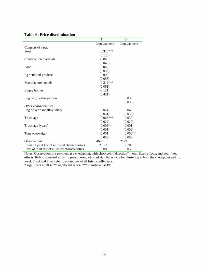
To verify the patterns shown in Figure 5, we estimate a price-discrimination equation.

The key advantage of the regression-based approach is that we can include checkpoint fixed

effects interacted with month fixed effects, to take into account the fact that different trucks

carrying different cargo may have traveled on different routes or at different times. Specifically,

we estimate the following equation:

'ci c i ciLOGPRICE Xα β ε= + + (10)

where each observation is a checkpoint-trip, 'iX are characteristics of the truck i and cα are

checkpoint * direction of travel * month fixed effects. Standard errors are simultaneously

clustered at both checkpoint level and trip level.

The results are reported in Table 6. Since the total value of truck contents was only

available for a subset of trips, in column (1) we use dummy variables for different types of truck

variables, whereas in column (2) we explicitly include the cargo value, limiting the sample to

those trips where the cargo value was reported. The results are consistent with Figure 5, showing

both the decreasing (and concave) relationship between truck age and price paid. The results in

column (2) also show the increasing relationship between cargo value and payments, although

the result is not statistically significant. The results also indicate higher payments for agricultural

produce, which may potentially be more time sensitive to transport than other cargo, and for

27 Though the average value per ton is not directly observable, the type of cargo is, and it is commonly known which types of cargo have higher or lower unit values.

- 32 -

steel, which is often of questionable legality. A joint F test of all characteristics shown in the

table reveals that these characteristics are jointly significant at the 1 percent level, indicating the

presence of substantial heterogeneity in prices that appears to be correlated with trucks’ ability to

pay. These results are in the same spirit as Svensson (2003), who also found that firms with

higher ability to pay do in fact pay higher bribes.

The social welfare consequences of price discrimination at checkpoints depends on

whether the total amount of corruption is affected by the ability to price discriminate. If the total

amount of corrupt revenue from bribes at weigh stations is fixed (for example, through some

type of political constraint), allowing third-degree price discrimination unambiguously reduces

the dead-weight loss from corruption (Baumol and Bradford 1970 - see Appendix A for details).

The analogy here is to the Ramsey tax problem – with third degree price discrimination, officers

can extract a greater share of the revenue from those truckers whose demand is less elastic, thus

increasing overall efficiency. If, however, we assume that the officials at weigh stations are not

subject to a revenue constraint, so that they can adjust prices to maximize R, then the welfare

effects of third-degree price discrimination are theoretically ambiguous, and depend on the

specific shape of the demand curves.28

5.2. Weigh stations and second-degree price discrimination The analysis of price discrimination above focused on observable characteristics of the

trucks that are essentially exogenous – given that a firm has been hired to transport a given

cargo, and owns a given truck, those characteristics are not choice variables available to the firm.

One choice variable that is available to the firm, however, is the weight of the truck. For a given

28 If demand curves are linear, then allowing third-degree price discrimination and allowing R to adjust decreases efficiency (Schmalensee 1981). With more general demand curves, however, Schmalensee shows that the welfare impact of third-degree price discrimination is ambiguous.

- 33 -

amount of cargo to be transported, the trucking firm can decide how many trips to split the trip

into or, conversely, whether to combine multiple cargoes into a single trip on a heavier truck.

If there is unobservable heterogeneity in, for example, the fixed cost firms must pay for

each trip, officials at weigh stations may introduce a non-linear pricing scheme to extract

additional revenue from truck drivers with a higher willingness to pay to be overweight. These

non-linear pricing schemes should feature quantity discounts, so that the marginal bribe required

for each additional ton the truck is overweight decreases as the number of tons overweight

increases (Tirole 1988).

Does this type of price discrimination exist in this context? In general, the non-parametric

regressions shown in Figure 2 appear approximately linear, of if anything, convex rather than

concave. The one weigh station that seems to show statistically significant quantity discounts

(based on the bootstrapped confidence intervals presented in the figure) is Seumedam, where

there appear to be slight quantity discounts after about 15 tons overweight. However, this

quantity discounting is not particularly strong, and in fact the overall evidence seems more

supportive of convex pricing (i.e., increasing marginal costs), rather than concave pricing (i.e.

quantity discounts).

However, these simple graphs actually mask a more interesting pattern at the Gebang

weigh station, located in North Sumatra province on the Banda Aceh – Medan route. In fact,

trucks heading in the direction of Banda Aceh have two options for paying their fine at the weigh

station. If they simply arrive at the weigh station, they pay a high marginal cost for being

overweight – regressions indicate that they pay approximately Rp. 11,000 (US $1.20) per ton

overweight for each ton over 10 tons overweight, plus a fixed fee of approximately Rp. 170,000

(US $18.50). If, on the other hand, they purchase a date-stamped coupon from a criminal

- 34 -

organization as they leave Medan for about Rp. 150,000 (US $16.30), when they arrive at the

weigh station they can turn the coupon in and pay a flat fee of approximately Rp. 50,000 (US

$5.50) to the weigh station attendants, for a total payment of Rp. 200,000 (US $21.70),

regardless of how overweight they are. Facing this schedule, drivers more than 16 tons

overweight should prefer the high fixed-fee, low marginal-cost scheme, whereas those less than

16 tons overweight should prefer the low fixed-fee, high marginal-cost scheme.

Figure 6 shows non-parametric locally-weighted regression estimates of the prices truck

drivers pay at Gebang (including the price of the coupon), separately depending on whether they

have purchased the coupon or not. The patterns visible in Figure 6 confirm that the existence of

two very different pricing schedules with a break-even line around 16 tons.

Table 7 investigates which trucks select into which fee schedule. Column (1) of Table 7

shows, quite surprisingly, that while heavier trucks are more likely to select into the high fixed

cost, low-marginal cost fee schedule, this effect is not statistically significant, and relatively

small in magnitude – moving from not being overweight at all to being 25 tons overweight, close

to the maximum reported, is associated with only an 8 percentage point higher probability of

choosing the high fixed cost, low-marginal cost fee schedule. However, column (2) indicates

that, consistent with the model, those with higher unobserved fixed costs (in the forms of higher

salaries for drivers) are much more likely to select into the high fixed cost, low marginal cost fee

schedule. Moreover, those drivers who get paid more also tend to carry heavier loads, so that in

column (3), when we instrument for truck weight with the log of the driver’s salary, we now get

a much larger (and statistically significant) coefficient on truck weight.

One way to reconcile these results is that drivers have some uncertainty about the amount

their truck actually weighs. Since they have to decide whether or not to buy the date-stamped

- 35 -

coupon before they depart Medan (and, therefore, before they reach the first weigh station), they

decide based on whether they are generally overweight or not. This would explain why factors

that predict whether they are overweight – such as the driver’s salary – have more predictive

power than the actual weight of the truck.29 This uncertainty could also explain why there are

two two-part tariffs, rather than a single non-linear tariff; in the presence of ex-ante uncertainty

about the weight of the truck and risk-averse truck drivers, this system of multiple two-part

tariffs can actually produce more revenue that a simple non-linear tariff payable at the weigh

station (Clay, et al. 1992, Miravete 2005). The contract offered is therefore most like that offered

on cell phone plans in the United States, where users who face an uncertain amount of usage

have to select ex-ante whether they prefer a high-fixed fee, low marginal cost contract or a low-

fixed fee, high-marginal cost contract.

The type of second-degree price discrimination practiced at the Gebang weigh station,

while it may be revenue maximizing for corrupt officials, exacerbates the inefficiencies caused

by corruption at weigh stations. In particular, quantity discounts further decrease social

efficiency by moving from a linear (or even possible convex) bribe schedule to a concave bribe

schedule – exactly the opposite of the true social costs from driving overweight.

An interesting question is why this contract occurs only at the Gebang weigh station, and

only heading towards Aceh. First, given the more intensive scrutiny at Seumedam discussed

above, operating these more complex bribe contracts may not be feasible. Second, in all of the

routes except the route from Medan – Banda Aceh, most trucks travel as part of an organized

convoy. As a result, virtually all of the trucks on these routes have already paid a fixed fee for

the journey, which may make offering the type of contracts offered at Gebang more difficult.

29 It is also possible that there is classical measurement error in the driver’s estimate of the truck’s weight reported to the surveyor, in which case using IV would also increase the point estimates.

- 36 -

Understanding the precise circumstances that enable these complex arrangements to evolve is an

important direction for future work.

6. Conclusion This paper has examined the degree to which corrupt officials behave like firms. We

accompanied truck drivers on 304 trips transporting goods to and from the Indonesian province

of Aceh. During these trips, we observed a total of more than 6,000 bribes and other illegal

payments to police, military officers, and officials at weigh stations, or about 20 such payments

per trip. These payments averaged about 13% of the cost of each trip, more than the total wages

received for the trip by the truck driver and his assistant.

Using this data, we showed that the patterns of bribes paid conform to predictions of

standard models of pricing behavior from industrial organization. During the period under study,

the military staged a staggered withdrawal from Aceh province as part of a peace agreement with

the GAM rebel group. We document that this withdrawal led to a dramatic reduction in the

number of checkpoints at which trucks in Aceh had to stop to pay bribes. In response to this, we

show that average bribes paid at checkpoints on the remainder of the route increased, consistent

with double-marginalization in a chain of decentralized monopolies.

We also take advantage of the fact that we observed each payment directly to examine

how bribes are negotiated. Prices are not posted, nor do corrupt officials typically ask for a given

amount; instead, most of the time the truck driver simply offers an amount to the officer at the

checkpoint, who decides whether to accept it or to decline and ask for a higher price. Although

almost the vast majority of initial offers are accepted, we show that the equilibrium amount paid

nevertheless reflects the relative bargaining power of the two parties. For example, factors that

increase the bargaining power of the officer manning the checkpoint, such as whether he is

- 37 -

brandishing a gun, and the number of officers who are visible and could provide backup if

trouble arose, increase the equilibrium payment. Given the presence of bargaining, we then show

that bribes paid per checkpoint increase as the trip nears its destination, consistent with ex-post

hold-up along a chain of monopolies.

Finally, we showed that, even though corruption is illegal, complex systems can evolve in

order to achieve greater levels of price discrimination. We document the existence of price

discrimination based on observable characteristics, such as age of the truck and the cargo being

carried, so that trucks with characteristics that indicate higher willingness-to-pay are indeed

charged higher bribes. Moreover, we show that at one of the four weigh stations on the route, a

criminal organization appears to have partnered with weigh station officials to introduce a menu

of two-part tariffs. This suggests the barriers posed by the fact that corruption is illegal are not

sufficient to prevent complex pricing schemes involving multiple transactions.

The results here have several implications for anti-corruption policy. First, the double-

marginalization shown here implies that decentralized corruption can result in higher bribes

charged than if corruption was centralized. If that is the case, tackling corruption at the top of an

organization could actually lead to increases in total bribes paid, if the number of bribe takers on

the ground remains the same but their coordination system is undermined. Second, it suggests

that in many cases, simple policies such as limiting the number of police may lead to less

corruption. This is particularly true when the current equilibrium involves bribes that are paid to

traffic police regardless of whether a law is broken, as it is here. This was not a priori obvious –

for example, if pricing was centralized, prices would have simply adjusted and the policy would

have had no effect. There could also have been entry of criminal organizations to extract bribes

at checkpoints instead of the police. While the results suggest that the simple policy of reducing

- 38 -

the number of traffic police is partially effective at reducing bribes, endogenous responses from

remaining police officers partially offset the gains obtained by having fewer officers on the

streets.

Although the economic mechanisms identified in this paper are likely to be general, the

degree of centralization or decentralization of bribes will clearly vary according to the context.

For example, a pilot survey conducted by the authors in March 2005 on the road between

Jakarta, the capital of Indonesia, and Bandung, the capital of nearby West Java province, found

that – in contrast to Aceh – the vast majority of extortion payments made by truck drivers on the

Bandung – Jakarta route were in the form of routine monthly payments to police officials and

affiliated criminal organizations, with relatively little collected at checkpoints. One interpretation

of this phenomenon is that the corrupt officials in West Java had managed to centralize

collection of bribes precisely in order to overcome the double marginalization problem

demonstrated in this paper. Understanding the circumstances that allow corruption to be

coordinated in this way is an important direction for future research.

- 39 -

References AASHO. “Road Test Report 5: Pavement Research.” Highway Research Board Special Report

#61 (1961).

Baumol, William J., and David F. Bradford. “Optimal Departures from Marginal Cost Pricing.” American Economic Review 60, no. 3 (1970): 265-83.

Blanchard, Olivier, and Michael Kremer. “Disorganization.” Quarterly Journal of Economics 112, no. 4 (1997): 1091-126.

Borenstein, Severin, and Nancy L. Rose. “Competition and Price Dispersion in the Us Airline Industry.” Journal of Political Economy 102 (1994): 653.

Bresnahan, Timothy F., and Peter C. Reiss. “Dealer and Manufacturer Margins.” RAND Journal of Economics 16, no. 2 (1985): 253-68.

Cameron, A. Colin, Jonah B. Gelbach, and Douglas L. Miller. “Robust Inference with Multi-Way Clustering.” NBER Technical Working Paper #327 (2006).

Clay, Karen B., David S. Sibley, and Padmanabhan Srinagesh. “Ex Post Vs. Ex Ante Pricing: Optional Calling Plans and Tapered Tariffs.” Journal of Regulatory Economics 4, no. 2 (1992): 115-38.

Dahl, Carol. “A Survey of Oil Product Demand Elasticities for Developing Countries.” OPEC Review 18, no. 1 (1994): 47-66.

Di Tella, Rafael, and Ernesto Schargrodsky. “The Role of Wages and Auditing During a Crackdown on Corruption in the City of Buenos Aires.” Journal of Law and Economics 46, no. 1 (2003): 269-92.

Fan, Jianqing. “Design-Adaptive Nonparametric Regression.” Journal of the American Statistical Association 87, no. 420 (1992): 998-1004.

Fisman, Raymond, and Shang-Jin Wei. “Tax Rates and Tax Evasion: Evidence from 'Missing Imports' in China.” Journal of Political Economy 112, no. 2 (2004): 471-500.

Foster, David. “Sumatra Region Roads Project: Technical Assistance on Road Traffic Safety and Vehicle Weights and Dimension, Enforcement Component.” World Bank (2005).

Grossman, Sanford J., and Oliver D. Hart. “The Costs and Benefits of Ownership: A Theory of Vertical and Lateral Integration.” Journal of Political Economy 94, no. 4 (1986): 691-719.

Hart, Oliver D., and John Moore. “Property Rights and the Nature of the Firm.” Journal of Political Economy 98, no. 6 (1990): 1119-58.

Hsieh, Chang-Tai, and Enrico Moretti. “Did Iraq Cheat the United Nations? Underpricing, Bribes, and the Oil for Food Program.” Quarterly Journal of Economics 121, no. 4 (2006).

- 40 -

McMillan, John, and Pablo Zoido. “How to Subvert Democracy: Montesinos in Peru.” Journal of Economic Perspectives 18, no. 4 (2004): 69–92.

Miravete, Eugenio J. “The Welfare Performance of Sequential Pricing Mechanisms.” International Economic Review 46, no. 4 (2005): 1321-60.

Newey, Whitney K., and Kenneth. D. West. “A Simple, Positive Semi-Definite, Heteroskedasticity and Autocorrelation Consistent Covariance Matrix.” Econometrica 55, no. 3 (1987): 703-08.

Olken, Benjamin A. “Monitoring Corruption: Evidence from a Field Experiment in Indonesia.” NBER Working Paper #11753 (2005).

Pitafi, Basharat A. K. “Elasticity of Fuel Consumption in Pakistan: An Econometric Study.” University of Hawaii (2004).

Reinnika, Ritva, and Jakob Svensson. “Local Capture: Evidence from a Central Government Transfer Program in Uganda.” Quarterly Journal of Economics 119, no. 2 (2004): 679-705.

Schmalensee, Richard. “Output and Welfare Implications of Monopolistic Third-Degree Price Discrimination.” American Economic Review 71, no. 1 (1981): 242-47.

Shepard, Andrea. “Price Discrimination and Retail Configuration.” Journal of Political Economy 99, no. 1 (1991): 30-53.

Shleifer, Andrei, and Robert W. Vishny. “Corruption.” Quarterly Journal of Economics 108, no. 3 (1993): 599-617.

Spengler, Joseph J. “Vertical Integration and Antitrust Policy.” Journal of Political Economy 58, no. 4 (1950): 347-52.

Svensson, Jakob. “Who Must Pay Bribes and How Much? Evidence from a Cross Section of Firms.” Quarterly Journal of Economics 118, no. 3 (2003).

Tajima, Yuhki, Patrick Barron, Benjamin A. Olken, and Zejd Muhamad. “Trucking and Illegal Payments in Aceh: From War Economy to Peace Economy.” World Bank (2006).

Tirole, Jean. The Theory of Industrial Organization. Cambridge, Massachusetts: MIT Press, 1988.

Varian, Hal R. “Price Discrimination.” In Handbook of Industrial Organization, edited by Richard Schmalensee and Robert Willig, 597-654: Elsevier, 1989.

Yang, Dean. “Integrity for Hire: An Analysis of a Widespread Customs Reform.” University of Michigan (2006).

- 41 -

Appendix A: Proofs Proof of claims in Section 4.1.1: First, to show that 0P

n∂

>∂

, note that from equation (3) we know that, in

equilibrium, ( )P nε = − . It follows directly from the implicit function theorem that if ( )' 0Pε < then 0Pn

∂>

∂.

Second, we are interested 2

P Pn Pn nn n

∂∂ −

∂=∂

. Using the implicit function theorem on (3), we can see that ( )1

'Pn Pε

∂ −=

∂,

so ( )'

Pnnsign sign P

n Pε

⎧ ⎫∂ ⎧ ⎫⎪ ⎪ ⎪= − −⎨ ⎬ ⎨∂ ⎪ ⎪⎪ ⎪ ⎩

⎩ ⎭

⎪⎬⎭

. Using the fact that ( )P nε = − in equilibrium, we know that

( )( )'

PPnsign sign P

n Pεε

⎧ ⎫∂ ⎧ ⎫⎪ ⎪ ⎪=⎨ ⎬ ⎨∂ ⎪ ⎪⎪ ⎪ ⎩

⎩ ⎭

⎪− ⎬⎭

. So, to show that 0

Pnn

∂<

∂, we need to show that

( )( )'

1P P

Pεε

> . Recall that

( ) ( )( )

'q P PP

q Pε = , which implies that ( )

( ) ( ) ( )( )

2

2

'' ' ''

q P P q P q P PP

q Pε

+ − ⎡ ⎤⎣ ⎦=⎡ ⎤⎣ ⎦

. So, we need to show that

( )( )

( ) ( ) ( )( )( )( )

2

2

'' ' '

'1

'

q P P q P q P PP

q PP Pq P PP

q P

εε

+ − ⎡ ⎤⎣ ⎦⎡ ⎤⎣ ⎦= > , or equivalently, that

( )( ) ( ) ( )

( )( )

'' '1 1'

q P P q P Pq P q P q P q P

+ − > . Since

( )( )

'1

q P Pn

q P− = > , it suffices to show that

( )( ) ( ) ( )

'' 1 0'

q P Pq P q P q P

+ > , or, equivalently, that ( )( )

''1 0

'q P Pq P

+ > . For this

to be true it is sufficient that ( )'' 0q P ≤ since ( )' 0q P < . Proof of claims in Section 4.1.2: To solve the model, we take the set of payments pi as fixed, start at the last checkpoint, and work backwards. At the last checkpoint N, if an agreement between the officer manning the checkpoint and the truck driver is reached, the surplus from reaching an agreement is 1 - pN. This is because the cargo is now worth 1 if the trip is completed as opposed to 0 if it was confiscated, but pi must be paid to the boss of the checkpoint. The officer manning the checkpoints therefore receives ( )1 Npα − , and the truck driver retains the

surplus ( ) . The total bribe we observe includes the amount the officer keeps and the amount he will

pass on to his boss, i.e.,

(1 1 Npα− − )( )1N Nb pα α= − + .

At the previous checkpoint (N-1), a similar bargaining game takes place, except that now, the surplus from agreement is reduced by the amount that will have to be paid at checkpoint N. Applying this logic and working backwards, the total surplus the driver retains after passing checkpoint n is

( ) ( )11 1N

N n j n 1j

j npα α− + − +

=

− − −∑ (11)

and the bribe paid at checkpoint n is

(12) ( ) ( ) ( )1

1 1 1N

N n j nn

j n

b α α α α− −

= +

⎡ ⎤= − − − + −⎢

⎣ ⎦∑ j np p⎥

Given that these are the bribes that will be paid in equilibrium, the demand curve is now based on the total bribes paid, i.e.

- 42 -

( ) ( )1

1 1 1N

N jj

jq α α

=

⎛ ⎞− − + −⎜

⎝ ⎠∑ p ⎟

j

(13)

Knowing this, the bosses at checkpoints choose their prices to maximize the revenue they receive. The first-order condition for the boss at checkpoint n is

( ) ( ) ( ) ( ) ( )1 1

1 1 1 1 ' 1 1 1N N

N j n Nj n j

j j

q p p qα α α α α= =

⎛ ⎞ ⎛ ⎞− − + − = − − − + −⎜ ⎟ ⎜

⎝ ⎠ ⎝ ⎠∑ p ⎟∑ (14)

Defining P to be the total price, we have that

( )

( )11 n

n

PPp

ε

α= −

− (15)

Note that as 0α → , so that the officer has no bargaining power, (15) reduces exactly to the first-order condition in the simpler model, i.e., the condition in equation (3). We can now show the results given in the text. First, to show that total bribe paid is increasing as the trip goes along, note that from (15), in equilibrium the expression ( )1 n

npα− must be constant for all checkpoints n. This immediately implies that is increasing with n. Using this fact, equation np (12), combined with the fact that all are positive, implies that the total bribe paid at each checkpoint is also increasing in n.

np

What remains to show is that the double-marginalization effects demonstrated in Section 4.1.1 still arise in

this more complex framework. First, we want to show that 0PN∂

>∂

. To do this, note that from (15) we know that

each price can be written as

( ) ( )1

n n

PpPα ε

= −−

(16)

Substituting into (13), we can see that the total price paid is equal to

( ) ( ) ( ) ( )1

1 1 1 1N

N

j

PPP P

α αε ε=

= − − − = − − −∑ N PN (17)

Applying the implicit function theorem to (17), we get that 0PN∂

>∂

if ( )' Pε 0< , which was assumed. Finally,

we need to show that prices at individual checkpoints decrease with N. Taking each checkpoint as fixed, consider the case where we add a checkpoint to the end – i.e., we increase N and see what happens to prices at checkpoint n. Substituting (16) into (12) and rearranging terms, we see that

( )

( ) ( )( ) ( )1 1

1N

n n

Pb NP

α α αεα

1n⎡ ⎤

= − + − −⎢ ⎥− ⎢ ⎥⎣ ⎦

(18)

As N increases, we know that decreases. Also, we just showed that as N increases P increases. Since ( )1 N nα −−

1N

α < by assumption, ( )( )1 0N nα − − < , so the whole second term will be decreasing in N if ( )

0

PP

Pε

∂>

∂, or

equivalently, if

( )( )'

0

q Pq P

P

∂>

∂. Taking derivatives, a sufficient condition is that q is concave, i.e., ( )'' 0q P < ,

although once again a weaker condition that q is not too convex is sufficient. Second, consider the case where we add a checkpoint to the beginning of the trip, i.e., we add a checkpoint

at 0. For a given checkpoint n, all of the terms in (18) remain the same except P, which we know increases. By the same logic as before, this implies that decreases. Since adding a checkpoint either before or after a checkpoint n decreases the bribe paid at n, we can conclude that adding an additional checkpoint decreases the price at all existing checkpoints.

nb

- 43 -

Proof of claims in Section 4.3: At the last checkpoint, the surplus from agreement is 11 b− , where is pre-determined. Nash bargaining therefore implies that

1b

( )2 1b α= − 1b , so the final payoff to the driver is equal to

( )11 1b α− − − 1b . At the first checkpoint, Nash bargaining implies that

( ) ( ) ( )( )1

1 1 1arg max ln 1 ln 1 1b

b b bα α α= + − − − 1b− (19)

i.e., that 1b α= . Substituting in for at the second checkpoint yields that 1b ( )2 1b α α= − , so . Solving the

equivalent problem in 3 periods checkpoints yields

2b b< 1

( ) ( ){ }21 2 3, 1 , 1b b bα α α α α= = − = − , so it is still the case that

j kb b> if . j k< Proof of claims in Section 5.1: We want to minimize dead-weight loss such that we raise a fixed amount of revenue R. Suppose there are two types, i.e., we want to solve

( ) ( ) ( ) ( )1 21 2

0 0

1 2 1 1 1 2 2 2,min s.t.

p pp pq p dp q p dp p q p p q p R+ +∫ ∫ = (20)

Writing down the Lagrangian for this maximization problem, taking derivatives, and re-arranging the derivatives of the Lagrangian with respect to and immediately yields the result that, at the optimum, 1p 2p

( )( )

( )( )

' '1 1 1 2 2 2

1 1 2 2

q p p q p pq p q p

= (21)

i.e., the prices are set such that the elasticities of demand for the two types are equal. Since this is also precisely the rule used in third-degree price discrimination, we can conclude that third-degree price discrimination minimizes the dead-weight loss if revenue remains equal. In fact, for any amount of revenue to be raised, third-degree price discrimination, which equates the elasticities for the two types of goods, is the most efficient way to raise that amount of revenue.

- 44 -

Table 1: Summary statistics (1) (2) (3) Both roads Meulaboh Road Banda Aceh Road Total expenditures during trip (Rp.) 2,901,345 2,932,687 2,863,637

(725,003) (561,736) (883,308) Bribes, extortion, and protection payments 361,323 415,263 296,427

(182,563) (180,928) (162,896) Payments at checkpoints 131,876 201,671 47,905 (106,386) (85,203) (57,293) Payments at weigh stations 79,195 61,461 100,531 (79,405) (43,090) (104,277) Convoy fees 131,404 152,131 106,468 (176,689) (147,927) (203,875) Coupons / protection fees 18,848 - 41,524

(57,593) (0) (79,937) Fuel 1,553,712 1,434,608 1,697,010 (477,207) (222,493) (637,442) Salary for truck driver and assistant 275,058 325,514 214,353 (124,685) (139,233) (65,132) Loading and unloading of cargo 421,408 471,182 361,523 (336,904) (298,246) (370,621) Food, lodging, etc 148,872 124,649 178,016 (70,807) (59,067) (72,956) Other 140,971 161,471 116,308

(194,728) (236,202) (124,755) Number of checkpoints 20 27 11 (13) (12) (6) Average payment at checkpoint 6,262 7,769 4,421 (3,809) (1,780) (4,722) Number of trips 282 57 191 Notes: Standard deviations in parentheses. Summary statistics include only those trips for which salary information was available. All figures are in October 2005 Rupiah (US $1 = Rp. 9,200)

- 45 -

Table 2: Impact of number of checkpoints in Aceh on bribes in North Sumatra

(1) (2) (3) (4) (6) OLS OLS OLS IV OLS

Panel A: Log total payments Log expected checkpoints -0.736*** -0.695*** -0.643*** -0.782*** -1.107** on route (0.065) (0.069) (0.237) (0.131) (0.442) Sample Meulaboh Meulaboh Meulaboh

Pre-Press Conf.

Meulaboh Both Routes

Truck controls No Yes Yes Yes Yes Common time effects None None None None Cubic Observations 161 144 90 144 249 Test elas = 0 0.00 0.00 0.01 0.00 0.81 Test elas = -1 0.00 0.01 0.22 0.33 0.01

Panel B: Log average payment at checkpoint Log expected checkpoints -0.545*** -0.580*** -0.684*** -0.788*** -0.808*** on route (0.157) (0.167) (0.257) (0.217) (0.196) Sample Meulaboh Meulaboh Meulaboh

Pre-Press Conf.

Meulaboh Both Routes

Truck controls No Yes Yes Yes Yes Common time effects None None None None Cubic Observations 1941 1720 1069 1720 2715 Test elas = 0 0.00 0.00 0.01 0.00 0.33 Test elas = -1 0.00 0.00 0.13 0.09 0.00 Notes: In Panel A, observation is a trip, dependent variable is log total payments in North Sumatra province, and robust Newey-West standard errors allowing for up to 10 lags are included in parentheses. In Panel B, observation is a payment at a checkpoint, dependent variable is log payment at the checkpoint, sample is limited to North Sumatra province only, all specifications include checkpoint * direction of travel fixed effects, and robust standard errors in parentheses, adjusted simultaneously for clustering at the checkpoint and trip level. Truck controls are dummies for 6 types of contents, log driver’s monthly salary, truck age and truck age squared, and number of tons truck is overweight; these characteristics are examined in more detail in Table 6. The instrument in column (4) is the log number of troops remaining in Aceh in the districts covered by the Meulaboh route. Log expected checkpoints is calculated as discussed in text. * significant at 10%; ** significant at 5%; *** significant at 1% Table 3: Impact of number of checkpoints on total payments in district

(1) (2) (3) (4) OLS IV (troops) OLS IV (troops)

Log expected checkpoints in 0.663*** 1.522*** 0.586*** 0.786** District (0.081) (0.390) (0.082) (0.359) Sample Meulaboh Meulaboh Both Routes Both Routes Observations 1090 1026 1435 1363 Test elas = 0 0.00 0.00 0.00 0.55 Test elas = 1 0.00 0.18 0.00 0.03 Notes: One observation for each district encountered on each trip, with trip fixed effects and district*direction of travel fixed effects. Dependent variable is log of total amount paid in bribes in district. The instrument in column (2) is the log number of troops remaining in district. Robust standard errors in parentheses, adjusted simultaneously for clustering at the district * quarter and trip level. * significant at 10%; ** significant at 5%; *** significant at 1%

- 46 -

Table 4: Bargaining vs. fixed prices

(1) (2) Log Payment Negotiate dummy

Gun visible 0.166*** 0.042*** (0.056) (0.015)

Number of people at 0.047*** 0.017*** Checkpoint (0.009) (0.004) Observations 5198 5165 Notes: Observation is a payment at a checkpoint, with trip fixed effects, checkpoint*direction* month interval fixed effects. Robust standard errors in parentheses, adjusted for clustering at the checkpoint level. * significant at 10%; ** significant at 5%; *** significant at 1% Table 5: Sequential bargaining and increasing prices

(1) (2) Mean percentile 0.145*** -0.178

(0.045) (0.225) Sample Meulaboh Banda Aceh Observations 4190 1089 Notes: Observation is a payment at a checkpoint, with trip fixed effects and checkpoint * month interval fixed effects. . Robust standard errors in parentheses, adjusted for clustering at the checkpoint level. * significant at 10%; ** significant at 5%; *** significant at 1%

- 47 -

Table 6: Price discrimination

(1) (2) Log payment Log payment

Contents of truck Steel 0.326***

(0.123) Construction materials -0.060

(0.045) Food 0.042

(0.035) Agricultural produce 0.092

(0.058) Manufactured goods -0.212***

(0.061) Empty bottles -0.121

(0.451) Log cargo value per ton 0.039

(0.030) Other characteristics Log driver’s monthly salary 0.024 0.040

(0.031) (0.039) Truck age 0.063*** 0.030

(0.022) (0.029) Truck age (years) -0.003** -0.001

(0.001) (0.002) Tons overweight -0.001 0.006**

(0.003) (0.003) Observations 4636 2179 F stat on joint test of all listed characteristics 29.12 7.78 P val of joint test of all listed characteristics 0.00 0.05 Notes: Observation is a payment at a checkpoint, with checkpoint*direction* month fixed effects, and hour fixed effects. Robust standard errors in parentheses, adjusted simultaneously for clustering at both the checkpoint and trip level. F stat and P val refer to a joint test of all listed coefficients. * significant at 10%; ** significant at 5%; *** significant at 1%

- 48 -

- 49 -

Table 7: Who selects into high fixed cost contract?

(1) (2) (3) OLS OLS IV

Tons overweight 0.003 0.039** (0.010) (0.019)

Log driver’s monthly salary 0.305** (0.119)

Constant 0.495*** -4.018** 0.074 (0.138) (1.760) (0.210)

Observations 47 47 47 R-squared 0.00 0.09 Notes: Observation is a trip, and sample is restricted to all trips on the Medan – Banda Aceh route headed in the direction of Banda Aceh, as coupons are only for sale on this route and only for this direction of travel. Column (1) and (2) are estimated as linear probability models using OLS; column (3) is estimated as a linear probability instrumental variables using 2SLS. Robust standard errors in parentheses. Non-linear probit and instrumental variables probit models produce qualitatively results. All columns drop two outliers – the highest observation on weight and the highest observation on salary. Including these observations strengthens the statistical significance of the results in columns (2) and (3). * significant at 10%; ** significant at 5%; *** significant at 1%

Figure 1: Routes

Figure 2: Payments at weigh stations

050

100

150

200

250

300

Pay

men

t (R

p. th

ousa

nds)

0 10 20 30 40Tons overweight

Banda Aceh − Gebang

050

100

150

200

250

300

Pay

men

t (R

p. th

ousa

nds)

0 10 20 30 40Tons overweight

Banda Aceh − Seumedam

Banda Aceh0

5010

015

020

025

030

0P

aym

ent (

Rp.

thou

sand

s)

0 10 20 30 40Tons overweight

Meulaboh − Doulu

050

100

150

200

250

300

Pay

men

t (R

p. th

ousa

nds)

0 10 20 30 40Tons overweight

Meulaboh − Sidikalang

Meulaboh

Notes: Each graph shows the results of a non-parametric Fan (1992) locally weighted regression, with the bandwidth equal to one-third of the range of the independent variable. Bootstrapped 95% confidence intervals are shown in dashes, where bootstrapping is clustered by trip. When the dashed lines are not shown, it indicates that the 95% confidence interval exceeds the y axis of the graph.

- 51 -

Figure 3: Impact of troop withdrawals on Meulaboh road

010

0020

0030

00T

roop

s

010

2030

4050

Ace

h

11/05 1/06 3/06 5/06 7/06

Num checkpoints in Aceh

010

0020

0030

00T

roop

s

1011

1213

N S

umat

ra11/05 1/06 3/06 5/06 7/06

Log total payments in North Sumatra

010

0020

0030

00T

roop

s

88.

59

9.5

10N

Sum

atra

11/05 1/06 3/06 5/06 7/06

Log average bribe paid in North Sumatra

Notes: Each observation is a trip on the route from Meulaboh - Medan. Dots on the left figure show the number of checkpoints in Aceh province on the trip. Boxes in the center show the log of total payments made in North Sumatra province, including payments at weigh stations. Triangles on the right figure show average prices paid at checkpoints in North Sumatra province on the trip. The solid line indicates the number of troops and police stationed in Aceh province at the time the trip began. The dashed line indicates the date of the April 4, 2006 press conference.

Figure 4: Payments by percentile of trip

−.1

−.0

50

.05

.1

0 .2 .4 .6 .8 1Share of trip completed

Meulaboh

−.1

−.0

50

.05

.1

0 .2 .4 .6 .8 1Share of trip completed

Banda Aceh

Notes: Each graph shows the results of a non-parametric Fan (1992) locally weighted regression, with the bandwidth equal to one-third of the range of the independent variable. Dependent variable is log payment at checkpoint, after removing checkpoint * month fixed effects and trip fixed effects. Bootstrapped 95% confidence intervals are shown in dashes, where bootstrapping is clustered by trip.

- 52 -

Figure 5: Price discrimination on observable characteristics 0

2000

4000

6000

8000

1000

0

0 5 10 15Truck age

020

0040

0060

0080

0010

000

14 15 16 17 18Log cargo value per ton

Notes: Each graph shows the results of a non-parametric Fan (1992) locally weighted regression, with the bandwidth equal to one-fifth of the range of the independent variable. Bootstrapped 95% confidence intervals are shown in dashes, where bootstrapping is clustered by trip. When the dashed lines are not shown, it indicates that the 95% confidence interval exceeds the y axis of the graph. Figure 6: Payments at Gebang weigh station

010

0000

2000

0030

0000

4000

00R

upia

h

0 5 10 15 20 25Overweight tons

Coupon

Gebang

Notes: locally-weighted regression of total amount paid on amount overweight. Cannot reject that slope of coupon line is zero, but can reject that slope of no coupon line is zero and can reject that two slopes are equal. 95%. Drops one observation that was more than 30 tons overweight, and observations from one surveyor who did not record whether the truck had paid the coupon or not.

- 53 -