The simulation of shock- and impact-driven flows with Mie-Gr¨ uneisen equations of state Thesis by Geoffrey M Ward In Partial Fulfillment of the Requirements for the Degree of Doctor of Philosophy California Institute of Technology Pasadena, California 2011 (Defended December 3rd, 2010)
Transcript
The simulation of shock- and impact-driven flows withMie-Gruneisen equations of state
4.10 Growth rate oscillation frequency for “heavy-to-light” Richtmyer-Meshkov instability 60
1
Chapter 1
Introduction
1.0.1 Shock-driven flows
1.0.1.1 Overview
The impulsive acceleration of a corrugated material contact by a shock wave is one of the most
fundamental research topics in the area of compressible flows. Applications for such research are
numerous and vast in complexity, ranging from supernovas to inertial confinement fusion (ICF)
to hypervelocity impacts in solids. Richtmyer [71] and Meshkov [53] were first to draw attention
to the topic, proposing a simple incompressible model that leads to a linear growth prediction
for the corrugation amplitude. A great deal of research has been performed on Richtmyer-Meshkov
instability since its introduction [14, 25, 33–35, 39, 41, 50, 60, 89, 93, 93–95, 98]. The present focus of
this investigation is on the role of the equation of state. A numerical comparison between simulations
of planar Richtmyer-Meshkov instability in fluids with Mie-Gruneisen equation of state derived from
shock Hugoniots of solids and perfect gases is undertaken. The majority of prior numerical studies
of Richtmyer-Meshkov instability have focused on the perfect gas equation of state. These studies
often have a constant specific heat ratio owing to challenges associated with the numerical modeling
of multiphase Mie-Gruneisen flows [2]. Presently, in Chapter 3 a low dissipation hybrid solver is
developed to address such numerical challenges created by the Mie-Gruneisen equation of state. The
solver is implemented as a patch solver in Caltech’s virtual test facility (VTF) software suite that
utilizes object-oriented C++ adaptive mesh refinement (AMROC) [15–17].
1.0.1.2 Richtmyer-Meshkov instability background
Two distinct variations of Richtmyer-Meshkov instability are commonly noted. The first, more
commonly studied, involves a shock wave that begins in a lighter fluid and travels until it reaches a
corrugated interface with a heavier fluid. Upon the shock interacting with the material contact, the
misaligned gradients of thermodynamic quantities cause baroclinic deposition of vorticity leading
to growth of the corrugation amplitude. Transmitted and reflected shock waves move away from
2
the post-shock corrugation. This situation, often denoted as “light-to-heavy” Richtmyer-Meshkov
instability, is schematically depicted in figure 1.1(a). To the right of the schematic, Figure 1.1(b), is
a wave diagram for the related zero-corrugation Riemann problem showing the position of the shocks
and material contact as a function of time. The frame of reference, as is the case for all simulations
presented here, is such that the interface is stationary post-shock for zero-corrugation amplitude.
Figure 1.2(a) depicts the second case of interest in which a reflected expansion wave occurs instead
of a shock. Although it is also possible to achieve a reflected shock for such cases, in general, a
reflected expansion wave occurs when the shock starts out in the heavy fluid. For this reason the
reflected expansion situation is referred to as “heavy-to-light” Richtmyer-Meshkov instability. For
such cases a phase reversal of the corrugation is also observed due to the difference in the direction
of the density gradient yielding baroclinic vorticity generation opposite in sign to that of the “light-
to-heavy” case. The wave diagram for the associated zero-corrugation problem is depicted in Figure
1.2(b). Due to the difference in the reflected wave created by the shock-corrugation interaction in
the above discussed situations, variation in the solution of these two fundamental cases is expected.
(a) (b)
Figure 1.1: (a) Schematic depiction of Richtmyer-Meshkov instability for the case in which the shock startsin the light fluid, resulting in perturbed reflected and transmitted shock waves. (b) Schematic depiction ofthe y-t diagram for the associated one-dimensional Riemann problem
1.0.1.3 Comparison study overview
In attempting to make comparison between flows with different equations of state it is useful to try
to create some level of flow similarity. A variety of theoretical and experimental work has been per-
formed on Richtmyer-Meshkov instability that yields insight into what would be required to achieve a
high level of similarity. From simple consideration of the associated one-dimensional Riemann prob-
lem it is clear that a set of nondimensional parameters involving corrugation wavenumber, shock
3
(a) (b)
Figure 1.2: (a) Schematic depiction of Richtmyer-Meshkov instability for the case in which the shock startsin the heavy fluid, typically resulting in a perturbed reflected expansion and transmitted shock waves. (b)Schematic depiction of the y-t diagram for the associated one-dimensional Riemann problem
speeds, speeds of sound, densities, shock Hugoniot slopes, and incident shock strength are important
for achieving similarity in the case of a small corrugation. The matching of all the quantities in any
such nondimensional set for flows with vastly different equations of state is not likely achievable.
This is the underlying motivation for the present study and comparison. For present purposes, in
spite of the impossibility of achieving full similarity, several key parameters are matched between
flows. The choice of these parameters is somewhat arbitrary, but provides a useful basis for com-
parison. The quantities matched are the post-shock Atwood ratio, a nondimensional pressure ratio
across the incident shock, the ratio of post-shock corrugation amplitude-to-wavelength ratio, and
time nondimensionalized by the Richtmyer growth rate prediction time constant. A parameter study
of two arbitrary Mach numbers of 1.5 and 2.5 in fluids with Mie-Gruneisen equations of state forms
a basis for comparison of single-mode instability. A matching set of initial conditions for perfect gas
flows is generated based on these two cases.
Results of the numerical investigation begin in Section 4.4 for two incident shock Mach numbers,
1.5 and 2.5 in the “light-to-heavy” case with a single-mode corrugation in fluids with Mie-Gruneisen
equation of state. For comparison purposes also examined is the equivalent matched perfect gas cases.
For both equations of state, amplitude and growth rate results are examined in detail in Section
4.4 followed by integral vorticity in Section 4.4.3 and corrugation centerline shortly post-shock in
Section 4.4.4. For a single incident Mach number of 2.5, in Section 4.5 next examined is a triple-
mode case with the three corrugation wave numbers related by the property that k1 = k2 + k3 and
k1h1 = k2h2 = k3h3. Instability amplitude and growth rate are again examined for both equations
of state in Section 4.5.1. Lastly, in Section 4.6 single-mode “heavy-to-light” Richtmyer-Meshkov
4
instability results are presented. Again two Mach numbers are utilized to compare amplitude and
growth rate in Section 4.6.1 as well as post-shock integral vorticity in Section 4.6.2 and centerline
distributions in Section 4.6.3 between equations of state.
1.0.1.4 Numerical methods background
In the presence of shocks and interfaces, compressible flows involve both smooth and nearly dis-
continuous features. In addition to the many challenges associated with simulating Euler flow of
perfect gases with such features, creation of a multiphase solver for linear shock-particle centered
Hugoniot Mie-Gruneisen equation of state must address several special difficulties. Firstly, whereas
many miscible gas mixtures can be well modeled by Dalton’s law of partial pressures, no single
simple multiphase miscible or immiscible mixture rule exists. Additionally, for multiphase flows
catastrophic phase-error driven oscillations can develop without proper numerical treatment [2].
Eulerian Cartesian mesh numerical methods that mitigate such oscillations by separating phases
have been proposed that use a pseudo physical mixture rule or a contact model [22, 57], but are
generally dissipative in multiphase regions. An alternative approach to modeling immiscible mul-
tiphase Mie-Gruneisen flows is to use an ad hoc fluid mixture rule and track additional variables
related to the equation of state [4, 81], which allows for more flexibility in the numerical approach
utilized. In Chapter 3 a new generalized set of limiters based on WENO [37, 48, 79] is developed
that allows for high-order Eulerian schemes to be blended with lower-order upwinding schemes in
a robust manner. In conjunction with an ad hoc material mixture Cartesian mesh method that
addresses phase-error oscillations [81], these limiters allow for the creation of a new hybrid scheme
that combines a high-order skew-symmetric kinetic-energy preserving center-difference [65] approach
in smooth flow regions with low-order upwinding at discontinuities for multiphase Mie-Gruneisen
flows.
1.0.2 Impact-driven flows
1.0.2.1 Overview
The focus of Caltech’s participation in the Predictive Science Academic Alliance Program (PSAAP)
program is the validation of simulations of hypervelocity impacts in metallic projectiles and targets.
In the spirit of this purpose a brief investigation of an extension of the ghost fluid method [8, 22] for
single phase free surface flows with linear shock-particle centered Hugoniot Mie-Gruneisen equation
of state is undertaken in Chapter 5. The method is first applied in a one-dimensional impact problem
with a simple erosion model for spallation. A corresponding rod impact problem is simulated in the
axisymmetric case. Finally, to demonstrate the potential further use of such a solver for hypervelocity
impacts in solids, the method is applied to study the three-dimensional axisymmetric impact of an
5
aluminum sphere and plate modeled as Mie-Gruneisen fluids.
1.0.2.2 Numerical methods background
Impact-driven flows with free surfaces present additional numerical challenges in a fixed grid Eulerian
setting. Whereas Lagrangian methods provide a natural approach to keeping track of the free surface
and applying traction conditions [21, 62], Eulerian solvers require interpolation of Cartesian mesh
data to apply traction conditions and advect the free surface. As was previously discussed, for
shock-driven flows a low-dissipation mixed-phase Eulerian solver approach can be utilized to study
problems with moderate material property variation between phases. However, such a approach
cannot be applied to free surfaces due to their inherently one-sided nature. Instead, the methods
required to properly treat vacuum-material interfaces are one-sided upwinding schemes. The ghost
fluid and volume of fluid (VOF) method were proposed independently to handle material interfaces,
but lend themselves to handle vacuum interfaces as well [22, 57].
For simplicity, although not even conservative in its original implementation, the ghost fluid
method is presently extended for fluid-vacuum simulations with the addition of an algorithm for
handling single cell sized voids. The ghost fluid method was originally proposed to address the
catastrophic oscillations that develop in mixed-phase flux-splitting schemes by separating the phases
through a scalar with a sign change referred to as a level-set [22]. For vacuum-interface problems
traction conditions can be achieved by tracing out tangent curves to the signed distance function and
the solving surface normal Riemann problems to determine ghost cell values. The signed distance
function must therefore be calculated periodically [22, 26, 75]. It is important that mechanical
information not traverse across small voids for proper treatment of such problems. To address this
issue an approach that subdivides the domain utilizing the signed distance function is introduced.
1.0.3 Eulerian solid mechanics
1.0.3.1 Overview
The fundamental difference between solids and fluids is the ability of solids to resist continuous
deformation under shear stresses. Therefore utilizing an isotropic stress Mie-Gruneisen equation
of state model should not be expected to give realistic results when shear is important. However,
many solids can only support a limited amount of anisotropic stress due to plasticity [66, 67, 91].
For this reason an isotropic stress model should be expected to capture at least some solution
features for many ductile solids under high compressive stress. In Chapter 6 an exploration of
the assumptions of the Mie-Gruneisen fluid equation of state are undertaken in the context of
comparison to elastic-plastic metals for several simulations. An Eulerian Cartesian mesh method is
utilized to simulate the elastic-plastic solids [30]. First, in one dimension a simple impact problem
6
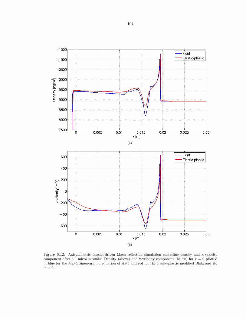
is modeled with elastic, elastic-plastic, and fluid Mie-Gruneisen models. Secondly, an axisymmetric
three-dimensional simulation is preformed of a two phase problem involving a semi-infinite length
copper cylinder surrounded by an aluminum slab struck by a semi-infinite aluminum slab. A Mach
disc is generated in the inner copper cylinder traveling along at the same speed as the planar shock
in the outer aluminum [11].
7
Chapter 2
The Mie-Gruneisen equation ofstate
In a completely general manner, an isotropic stress equation of state can be rigorously constructed
about a parametric reference state curve through an integral equation. Choosing to construct pres-
sure as a function of internal energy and density leads to the very convenient Gruneisen formalism
p(ρ, e) = pref (ρ) + ρ
∫ e
eref (ρ)
Γ(ρ, e′)de′, (2.1)
where pref (ρ) and eref (ρ) form a density parameterized reference state curve and Γ(ρ, e) is the
Gruneisen parameter defined by
Γ(ρ, e) =1ρ
∂p
∂e
∣∣∣ρ. (2.2)
A material is then well defined thermodynamically by pref (ρ), eref (ρ), and Γ(ρ, e). In practice,
whether analytic or tabulated, these three functions should, at a minimum, result in the thermody-
namic stability of the material modeled in state regions of interest [57].
2.0.4 Hugoniots as reference state curves
For the simulation of compressible flows involving shocks it is convenient to use shock Hugoniots
for reference state curves [36, 52, 73]. For many solids of interest, starting from state ρ0, p0, e0,
experimental data indicates that over a large range of shock strengths the relationship between shock
and particle speed is adequately approximated by a simple linear fit [36, 52, 73]
us = c0 + σup, (2.3)
where us is the shock’s speed, up is the post-shock particle speed, c0 is the unshocked medium’s
speed of sound, and σ is related to the unshocked medium’s isentropic derivative of the bulk modulus
8
Ks with respect to pressure
Ks = ∂ ln(p)∂ρ
∣∣∣s,
σ =(∂Ks∂p
∣∣∣s
+ 1)/
4.(2.4)
Utilizing (2.3) and the three Rankine-Hugoniot jump conditions for conservation of mass, momen-
tum, and energy,
ρ = ρ0us/(us − up),
p = p0 + ρ0usup,
e = e0 + 12 (p+ p0)(1/ρ0 − 1/ρ),
(2.5)
results in the internal pressure and energy parametrized as functions of density along the shock
Hugoniot [81],
pH
(ρ) = p0 +c20(1/ρ0 − 1/ρ)
[1/ρ0 − σ(1/ρ0 − 1/ρ)]2, (2.6)
eH
(ρ) = e0 +12
(pH
(ρ) + p0)(1/ρ0 − 1/ρ). (2.7)
Additionally, for many solids it is approximated that the Gruneisen parameter is given by [57]
Γ(ρ, e) = Γ0
(ρ0ρ
)q= Γ
H(ρ).
(2.8)
In terms of internal energy this is a first-order approximation to Γ(ρ, e) near the Hugoniot:
Γ(ρ, e) = Γ(ρ, eH
(ρ)) + ∂Γ∂e
∣∣∣ρ,e
H(ρ)
(e− eH
(ρ)) + ...
= ΓH
(ρ) +O(∆e).(2.9)
Thus the equation of state is a first-order approximation in internal energy near the central Hugoniot
with
p(ρ, e) = pH
(ρ) + ρΓH
(ρ)(e− eH
(ρ)). (2.10)
Generally, (2.6) and (2.7) are only valid for compressed states ρ > ρ0. For expanded states a
second-order isentropic continuation to the Hugoniot known as a Murnaghan isentrope is sometimes
used [57]:
pH
(ρ) =(p0 +
ρ0c20
4σ − 1
)( ρρ0
)4σ−1
− ρ0c20
4σ − 1, (2.11)
eH
(ρ) = e0 +∫ ρ
ρ0
pH
(ρ)ρ2
dρ. (2.12)
(2.13)
9
Table 2.1: Hugoniot constants for various materials. For further shock-particle Hugoniot constants refer to[36, 52, 73]
ρ0 p0 Γ0 c0 σ q T0
aluminum 2785 kg/m3 0.0 2.0 5328 m/s 1.338 1.0 298 KMORB 2660 kg/m3 0.0 1.18 2100 m/s 1.68 1.0 1673 K
molybdenum 9961 kg/m3 0.0 1.56 4700 m/s 1.43 1.0 1673 K
2.0.5 Equation of state limitations
Construction of a central Hugoniot utilizing the assumption of a linear shock-particle speed relation-
ship and Murnaghan isentrope extension for expanded states result in two notable limitations. First,
using a simple linear fit to the relationship between shock and particle speed causes a singularity in
the equation of state that results in a nonphysical maximum density
ρmax =ρ0
1− 1/σ, (2.14)
when σ > 1, as is typical for solids. Second, analysis of isentropes created by the extension of the
Hugoniot for expanded states via the Murnaghan isentrope demonstrates a non-physical minimum
pressure [90]:dp
dρ
∣∣∣s
= c1p
ρ2+ c2
1ρ2
+ c3ρ4σ−3 + c4ρ
4σ−2 (2.15)
along any isentrope when ρ < ρ0 and p < p0, where c1, c2, c3, and c4 depend on the central Hugoniot
constants. Integrating (2.15) from initial conditions ρi, pi, and si yields
p(ρ, si) = (pi + c2c1
)ec1(1/ρi−1/ρ) − c2c1
+ec1/ρ∫ ρρi
(c3ρ′4σ−3 + c4ρ
′4σ−2)ec1/ρ′dρ′.
(2.16)
When approached from the part of the p− ρ plane of physical interest, the limit
limρ→0
p(ρ, si)→ −c2c1
=−ρ0c
20
4σ − 1(2.17)
is obtained for all associated isentropes when σ > 1/2. Therefore no pressures lower than
pmin =−ρ0c
20
4σ − 1(2.18)
are attainable. With ρ0 > 0, c0 > 0, and σ > 0 it is clear that pmin < 0 is typical and therefore
negative pressure or tension is permissible. It is useful to place a tensile strength limitation when
tension is expected in a simulation. Additionally, positivity of absolute temperature must not be
violated. Taking constant specific heat for aluminum yields Figure 2.1, giving some face to the
expected p− ρ plane of validity.
10
Figure 2.1: Forbidden and allowed state regions of the Mie-Gruneisen equation of state formulated from alinear shock-particle speed central shock Hugoniot and Murnaghan isentrope extension for expanded states.The available states are bounded by negative temperature, a nonphysical minimum pressure, and a non-physical maximum density.
2.0.6 Mixture rules
Kinetic theory for ideal gas mixtures predicts that total pressure is described by partial pressure
summation [40]. For mixtures of perfect gases this law is easily applied to form an analytic equation
of state [85],
p = (1− γ)ρe, (2.19)
with
γ =n∑i=1
yicip
/ n∑i=1
yiciv (2.20)
where yi, cip, and civ are the ith components mass fraction and specific heats, respectively. Presently,
the above mixture rule for perfect gases is applied in simulations. However, for most real materials
such a simple theory for molecular interactions in mixtures does not exist. Owing to the complexity
inherent in providing a physical mixture model for real materials, previous works addressing the
simulation of multiphase flows typically assume discontinuous contact between materials, tracking
the contact [57] and applying some isentropic relaxation of phases to mechanical equilibrium or
smearing it with an ad hoc mixture rule [4, 81]. An ad hoc blending of parameters is currently used,
xmix0 =n∑i=1
ψi0xi0, (2.21)
11
where xi0 is replaced in the formula by the Hugoniot parameters, ρ0, p0, e0, Γ0, and σ of the ith
material. Although in principal this model is not physical, the weak convergence of solutions with
discontinuous interfaces should still result.
12
Chapter 3
Hybrid, center-difference, limitersolver
In the following sections the special difficulties associated with building a hybrid solver for multiphase
flows with Mie-Gruneisen equations of state are addressed. For Euler flows a continuous transition
from low-order upwinding at discontinuities to high-order low dissipation in smooth regions is desir-
able. A substantial amount of literature on hybrid solvers for perfect gases exist focusing on the use
of WENO interpolation [3, 29, 68]. WENO provides a very natural way to create a hybrid scheme for
hyperbolic partial differential equations in the way that it combines sub-stencils based on smooth-
ness measures in order to produce a low-order approximation at sharp features and high-order at
smooth solution regions. Designing the desired high-order stencil WENO becomes in smooth solu-
tion regions allows for dispersion relation matching to a high-order center-difference scheme for small
wave numbers [29]. However, these WENO methods commonly apply a flux-splitting reconstruction
approach that is conservative, but fails to prevent catastrophic oscillations [2] at contacts in many
Mie-Gruneisen fluids (see Figure 3.1), rendering such methods inadequate. An alternative primitive
variable WENO-reconstruction based Roe-Riemann solver [72] has been developed by Johnsen and
Colonius [38] that prevents such oscillations from developing in mixtures of perfect gases. However,
the stencil associated with any such Riemann solver is dependent on the flow locally and therefore
the dispersion relation is complex and does not lend itself to hybrid methodology. For multiphase
flows with Mie-Gruneisen equations of state Miller and Puckett [57] developed a volume of fluid ap-
proach that utilizes an approximate Riemann solver, again yielding no ideal stencil for smooth flows.
Likewise, Shyue [81] has extended Roe’s approximate Riemann solver for multiphase Mie-Gruneisen
flows. Attempts to form hybrid solvers through simple low-order smoothness measure-based blending
of schemes have been made for conservative flux-splitting solvers [3, 68].
Presently, in order to address the above issues, a blending methodology based on a norm of the
deviation of local smoothness dependent WENO-reconstruction weights has been developed [90]. In
devising an effective limiter similarities between WENO and classical flux and slope limiter type
13
(a) (b)
Figure 3.1: MORB-molybdenum Mach 1.5 single cosine mode perturbation Richtmyer-Meshkov instabilitysimulation by simple flux-splitting method exhibiting catastrophic oscillations. Initial density contour plot(a) and later time (b). The mixed phase region is spread over a large number of scales to demonstrate thatthe phenomenon is not grid scale generated. At later time the solution is polluted by oscillations driven byphase errors.
methods are exploited. Doing so yields a generalized limiter useful for smoothly blending a lower-
order upwinding Riemann solver and high-order center-difference scheme while maintaining high-
order convergence for smooth flows. To first explore the properties of the new limiter methodology
it is applied to the linear advection equation, building fourth and sixth-order schemes and providing
comparison to standard third and fifth-order WENO methods [37, 79]. A detailed description
of a spatially fourth-order finite-difference patch-solver for the multiphase Euler equations with
special consideration for the Mie-Gruneisen equation of state is then explored. The implementation
combines spatially fourth-order skew-symmetric kinetic-energy preserving center-difference and a
second-order WENO Roe-Riemann approach. Hybridization is achieved for the solver through Lax-
entropy conditions and gradient tolerances. The scheme is then initially demonstrated for solids
modeled by isotropic Mie-Gruneisen equations of state in one dimension. This is followed up by
applying the methodology in two dimensions with adaptive mesh refinement capabilities utilizing
the California Institute of Technology’s VTF AMROC software [15].
3.1 Hybrid limiter methodology
Hyperbolic conservation laws typically describe material behavior containing discontinuities and
smooth regions, two features best addressed by different numerical schemes. At discontinuities a
14
low-order upwinding scheme is ideal for preventing oscillations. Alternatively, in smooth regions
of the solution a low dissipation method, often in the form of a centered difference scheme, is
advantageous [3, 29, 68]. However, applying different schemes directly to different regions can lead to
oscillations in regions where schemes meet if their dispersion relations are not suitably well matched
[29]. To avoid this difficulty, it is important that the stencil associated with one of the schemes
tends toward the others in regions where the schemes will meet. Additionally, flows with mixtures
of real materials modeled by Mie-Gruneisen equations of state can develop disastrous oscillations
when treated numerically by a conservative flux-splitting numerical scheme [2]. A generalized limiter
approach presents a way to address the above issues simultaneously. In practice the success depends
heavily on how the limiter is defined. Typically the limiter is based on a measure of smoothness
locally. In reality it is difficult to achieve the desired result of the limiter method completely reducing
to the desired stencil. For this reason a separate set of criteria resulting in a sharp cutoff filtering
of the limiter is of practical use. In effect, all hybrid schemes may be formulated as limiter schemes
with sharp cutoff filtering of the limiter.
3.1.1 Limiter methodology
The Lax-Wendroff theorem [45, 46, 86] indicates proper weak solution convergence for hyperbolic
conservation laws can be obtained sufficiently by using a numerical scheme that maintains conser-
vation of certain variables. A practical approach to creating such a conservative scheme is to define
flux derivatives by a symmetric difference of midpoint reconstructions fj±1/2 of order at least k− 2,
∂f
∂x=fj+1/2 − fj−1/2
∆x+O(∆xk). (3.1)
Although primitive quantities are not conserved, the above methodology can be applied uniformly
in approximating all derivatives. Practical application of (3.1) then only requires a midpoint recon-
struction of quantities of interest, namely fluxes and primitives such as pressure and velocity.
A blending of multiple reconstruction schemes is appealing for achieving different stencils for
sharp and smooth features:
fj+1/2 = fkj+1/2 + Φ(frj+1/2 − fkj+1/2). (3.2)
Here Φ is a limiter used to achieve the desired blend of frj+1/2 and fkj+1/2, rth- and kth-order
midpoint reconstructions, respectively. Typically frj+1/2 is a low-order upwinding scheme and fkj+1/2
is a higher-order method with less dissipation (k > r). It is therefore desirable that Φ approaches
unity at discontinuities and tends toward zero in smooth regions. Furthermore, in order to maintain
kth-order global convergence when a smooth solution is present, it is important to use a limiter with
15
the property that
Φ ∝ ∆xβ , β ≥ k − r. (3.3)
Defining a good limiter of practical use is a complicated matter [45, 46, 86]. In the following section
a structured way to define a practical limiter for a kth-order scheme based on WENO weights is
presented.
3.1.2 WENO-weight-inspired limiters
Weighted essentially non-oscillatory (WENO) schemes represent a popular subcategory of solvers
for hyperbolic partial differential equations [37, 48, 79]. At a basic level of interpretation WENO
is merely polynomial interpolation by weighted hierarchy. For practical application to numerical
methods on evenly spaced Cartesian grid points, WENO focuses on the reconstruction of midpoint
values, forming a weighted combination of r first-order sub-stencil interpolations qrk that tend toward
an order 2r − 1 approximation q2r−1r−1 of function f at x = (j + 1/2)∆x in smooth regions:
fj+1/2 = q2r−1r−1 (fj−r+1, . . . , fj+r−1)
+r−1∑k=0
(wk − Crk)qrk(fj+k−r+1, . . . , fj+k)
=r−1∑k=0
wkqrk(fj+k−r+1, . . . , fj+k).
(3.4)
Here Ck represent ideal sub-stencil weighting and wk are variable weights dependent on local solution
character. The above reflects a slope-limiter-like approach to the reconstruction of midpoint values.
Although not directly in slope limiter form, it is not to difficult to design weights that yield classic
slope limiter or even ENO methods. More commonly weights are defined systematically by
wk =αk
r−1∑j=0
αj
, (3.5)
αk =Crk
(ε+ ISk)p, k = 0, 1, . . . , r − 1, (3.6)
where ISk is a sub-stencil smoothness measure, p and ε are chosen constants, and Crk is the desired
sub-stencil weight in smooth solution regions [37].
Noting that slope and flux limiter approaches are equivalent, it is instructive to re-arrange (3.4)
in a flux-limiter-like form
16
fj+1/2 = q2r−1r−1 (fj−r+1, . . . , fj+r−1)
+r−2∑k=0
φkqrk(fj+k−r+1, . . . , fj+k)
−r−2∑k=0
φkq2r−1r−1 (fj−r+1, . . . , fj+r−1).
(3.7)
A matrix relationship exists relating the flux limiters φk and classic WENO weights wk,
A(Cr) · φ = w − Cr. (3.8)
Taking a norm of the above yields a single generalized limiter,
Φ =‖ A ‖p ‖w − Cr‖p. (3.9)
It is not surprising that the limiter norm is directly proportional to a norm of the deviation of weights
from ideal. Equation (3.9) provides a generalized robust way for defining a limiter for high-order
schemes.
3.2 High-order implementation
3.2.1 Linear advection equation solver
To demonstrate application of equation (3.9) the methodology is first applied to the linear advection
equation,∂u
∂t+∂u
∂x= 0, (3.10)
creating spatially fourth and sixth-order schemes based on high-order center-differences and WENO
reconstruction Riemann solvers.
In constructing a fourth-order method a standard fourth-order center-difference is utilized,
uCD4j+1/2 = − 1
12(uj+2 + uj−1) +
512
(uj + uj+1), (3.11)
combined by limiter with a third-order WENO scheme uWENO3j+1/2 [48],
uj+1/2 = uCD4j+1/2 + Φ(uWENO3
j+1/2 − uCD4j+1/2), (3.12)
where the limiter is defined by,
Φ = ‖w − Cr‖2. (3.13)
17
Standard fifth-order WENO weights with r = 3 and preferred stencil coefficients C30 = 1/10,C3
1 =
6/10, C32 = 3/10 is utilized for evaluating the deviation norm of equation (3.13). In determining the
weights, the method described in [37] is followed with ε = 10−6, p = 2 and smoothness measures
IS0 =1312
(uj−2 − 2uj−1 + uj)2 +14
(uj−2 − 4uj−1 + 3uj)2,
IS1 =1312
(uj−1 − 2uj + uj+1)2 +14
(uj−1 − uj+1)2,
IS2 =1312
(uj − 2uj+1 + uj+2)2 +14
(3uj − 4uj+1 + 3uj+2)2.
(3.14)
Likewise, in constructing a sixth-order scheme the center-difference
uCD6j+1/2 =
160
(uj+3 + uj−2)− 215
(uj+2 + uj−1) +3760
(uj+1 + uj) (3.15)
is applied and combined by limiter with a fifth-order WENO method uWENO5j+1/2 [37],
uj+1/2 = uCD6j+1/2 + Φ(uWENO5
j+1/2 − uCD6j+1/2). (3.16)
It is possible to combine sixth-order center-difference with third-order WENO scheme and still
achieve sixth-order convergence for smooth solutions. However, doing so results in higher dissipation
at discontinuities. To construct Φ for the present sixth-order method from equation (3.9) the seventh-
order WENO preferred stencil coefficients and smoothness indicators with p = 5, for which the
equations are omitted and can be found in their original source [6], is used.
To form a complete numerical scheme from the above spatial discretization a temporal discretiza-
tion is then required. For testing purposes, fourth-order strong-stability-preserving Runge-Kutta
(SSP RK-4) temporal discretization [24] is applied,
q(1) = qn +12
∆tL(qn),
q(2) = qn +12
∆tL(q(1)),
q(3) = qn + ∆tL(q(2)),
qn+1 =13
(−qn + q(1) + 2q(2) + q(3)) +16
∆tL(q(3)),
(3.17)
3.2.2 Test problems
For the purposes of comparison the previously described fourth- and sixth-order methods, as well
as third- and fifth-order WENO methods, are applied to the linear advection equation in a periodic
domain −1 ≤ x ≤ 1 with initial conditions
u(x, t = 0) ={ 1, −3/4 < x < −1/4
e−300(x−0.5)2, otherwise.
(3.18)
18
Figure 3.2: Numerical solutions to the linear advection equation in a periodic domain achieved with spatiallythird and fifth-order WENO, present fourth and sixth-order WENO-inspired limiter methods, denoted bydiamonds and crosses, triangles and circles, respectively. Solution depicted at 2000th time step, CFL = 0.5and n = 100.
Numerical solutions are shown at the 2000th time step in Figure 3.2 for simulation with n = 100
points and CFL = 0.5. The present sixth-order scheme best captures the solution, retaining the
Gaussian’s peak with greater fidelity and having a slightly sharper approximation to the square
wave. Third-order WENO displays a heavily diffuse approximation to the square wave while the
sixth-order method remains the sharpest.
Table 3.1: Square wave L2 error norm and convergence order for t = 2 and CFL = 0.9.
Figure 3.3: MORB-molybdenum Mach 1.5 single-cosine-mode perturbation Richtmyer-Meshkov instabilitysimulation results exhibiting carbuncle-like features (t = 37 ms). (a) A nonphysical notch at the spike tipis visible. (b) Rotating the flow by 45 degrees with respect to the grid removes the notch.
Figure 3.4: MORB-molybdenum Mach 1.5 single-cosine-mode perturbation Richtmyer-Meshkov instabilitysimulation results with present H-correction for carbuncle implemented for t = 37 ms. The carbuncle likenotch observed in Figure 3.3 is smoothed over.
30
The corresponding added amount of dissipation is then
ηHi+1/2,j∆qi+1/2,j − ηHi−1/2,j∆qi−1/2,j
∆x, (3.62)
where ∆qj = qR− q
Lis the difference in biased stencil reconstructions [77]. The above correction
works adequately at removing the notch observed in Figure 3.3 when applied with a low-order
linear Riemann solver. However, the solver described currently is not a true linearization of the
Euler equations since the blending of nonlinear center-difference and Riemann reconstruction has
no definable corresponding left and right state or linearized Jacobian matrix A. To address these
issues a multidimensional H-correction to the limiter is applied,
ΦHi+1/2,j =(
Φ2i+1/2,j +max(Φ2
i,j+1/2,Φ2i,j−1/2,Φ
2i+1,j+1/2,Φ
2i+1,j−1/2)
)1/2
, (3.63)
amplifying the limiter at sonic points with large wave speed variation,
ΦH′i+1/2,j =( ηHi+1/2,j/|λ|
Hmax
|λ|Hmin/|λ|Hmax + ε
)1/2
ΦHi+1/2,j , (3.64)
which promotes dissipation through the steepest parts of shock waves where the limiter often drops
bellow the maximum, resulting is an undesirable region with low dissipation. Then added is an
amount of dissipation equal to
ΦHi+1/2,jηHi+1/2,j∆qi+1/2,j − ΦHi−1/2,jη
Hi−1/2,j∆qi−1/2,j
∆x. (3.65)
Doing so works reasonably well at mitigating the carbuncle-like notch (see Figure 3.4), but also
yields a considerable increase in overall numerical dissipation.
3.2.4 One-dimensional test problems
3.2.4.1 Simple wave
First, to demonstrate how the limiter method behaves on its own, the method is presently applied
without hybridization to a simple wave in a one-meter-long periodic slab of mid-ocean ridge basalt
(MORB). The initial conditions are continuous and periodic in nature, corresponding to states in
tension along the Murnaghan isentrope. For continuous initial conditions, the single-phase Euler
equations in one dimension yield the solution [42]
u(ρ) = ±∫c(ρ)ρdρ (3.66)
31
along characteristics defined in space and time from
x = t(u± c(u)) + f(u). (3.67)
From these transcendental equations, a simple periodic single-mode wave solution for isentropes of
a perfect gas can be found [42]. The solution is shown to become increasingly steep, resulting in the
formation of shock waves. For metals described by Mie-Gruneisen equations of state with reference
state curves given by a Hugoniot, an analytic equation for isentropes is not generally attainable.
However, the use of a Murnaghan isentrope for extending the equation of state for expanded states
provides a single isentrope in the form
p(ρ, s = s0) = Aρα +B. (3.68)
Solution to the Euler equations for this isentrope in terms of velocity is then
u(ρ) =2√αA
α− 1ρα−1
2 + const. (3.69)
For the initial conditions a simple sine wave for the initial velocity profile is taken,
u(x, t = 0) = U0 sin(kx),
f(u) = 1k sin−1(u/U),
(3.70)
with U0 = 60.34m/s, corresponding to a density variation of 2500.4 ≤ ρ ≤ 2659.7 kg/m3. Simulation
results are seen in Figure 3.5 and Figure 3.6 for CFL = 0.95 and ∆x = 0.01 m. For early times the
limiter remains relatively small, yielding very little numerical dissipation. As the shockwave begins
to form at the inflection point the limiter increases locally to introduce the desired character of the
upwinding Roe solver, maintaining a relatively smooth solution.
For smooth solutions such as the simple wave before a shock forms, with the use of fourth-
order SSP RK-4 temporal discretization, the numerical convergence rate of the presently described
methodology should be fourth-order. To demonstrate the convergence rate an approximation to the
L2 error norm in density is calculated at t = 0.5 ms for various numbers of points while maintaining a
fixed CFL of 0.95. Again, to isolate the numerical method this is done so without hybridization. The
results of the study are given in Table 3.2. The convergence order is seen to be mesh-size dependent,
asymptotically approaching the expected fourth-order rate of convergence as the number of points
increases.
32
Figure 3.5: Simple wave simulation density and limiter profiles at t = 0.5ms. Simulation CFL = 0.95 and∆x = 0.01m. The dashed line refers to the initial conditions. As the solution progresses in time the waveslowly begins to break, inducing a gradual increase in the limiter locally centered around the steepeninginflection point.
Figure 3.6: Simple wave simulation density and limiter profiles at t = 1ms. CFL = 0.95 and ∆x = 0.01m.The dashed line refers to the initial conditions. As time progresses and a shock forms the limiter increasesto introduce more dissipation locally, maintaining a relatively smooth flow on either side of the shock.
33
Table 3.2: Simple wave solution density L2 error norm and convergence order for t = 0.5ms. As the grid isrefined, the order of convergence is seen to approach the expected fourth-order value.
Next a single-phase test problem consisting of an impact between two slabs of aluminum in one
dimension [81] is considered. A semi-infinite slab of aluminum with zero stress, corresponding to
ρ0, p0, and e0 given in 2.1, travels leftward at 2000 m/s striking a pre-compressed semi-infinite slab
of aluminum with density ρ = 4000 kg/m3 and pressure p = 7.98 GPa. Both slabs are modeled as
fluids with a single Mie-Gruneisen equation with Hugoniots as reference state curves. The solution
to this Riemann problem consist of a reflected and transmitted shock along with a constant pressure
and velocity density jump between them.
Figure 3.7 presents results at t = 50 µs for simulation of the problem with 100 points and
an adaptively maintained CFL = 0.95. The density, velocity, and pressure all remain relatively
smooth. The limiter, plotted bottom right in Figure 3.7, demonstrates the necessary increase near
the reflected and transmitted shocks. At the density contact the limiter is slightly less active, a
desirable result that is a consequence of the nature of the limiter which decreases as numerical
diffusion smooths out the flow. Ideally a hybrid switching criteria would indicate when the center-
difference scheme is solely adequate to maintain the feature, however, this is hard to achieve this in
practice.
3.2.4.3 Mach 2.5 MORB-molybdenum shock-contact problem
A one-dimensional shock-contact multiphase test problem involving two semi-infinite slabs that make
diffuse contact at the origin is next simulated. To the left is molybdenum and the right MORB,
states corresponding to ρ0, p0, and e0. Mach 2.5 shock wave travels through the MORB to the left
starting from x = 0.5 m. The shock eventually reaches the origin, yielding a transmitted shock in
the molybdenum slab and reflected shock back into the MORB. The diffuse contact at the origin is
defined by smearing the initial mixture fraction
ψ(x, t = 0) =12
+12
tanh(βx), (3.71)
34
Figure 3.7: Results from a one-dimensional simulation of an aluminum impact problem with 100 points andCFL = 0.95 at t = 50 µs. The dashed line refers to initial conditions and the solid line to the exact solution.The limiter adjusts at the reflected and transmitted shocks and interface, maintaining solution smoothness.
35
where β = 50 m−1 was taken. The states through diffuse contact are given by the ad hoc mixture
rule (2.21).
To keep the contact well within the domain, the simulation is performed in an inertial frame
of reference that gives zero velocity between the reflected and transmitted shocks. Results for 100
points and adaptively maintained CFL of 0.95 at t = 0.18µs are seen in Figure 3.8. Again it is
observed that the density, velocity, pressure, and initial mixture fraction maintain smooth profiles.
Figure 3.8: Mach 2.5 MORB-molybdenum shock-contact problem density, velocity, pressure, and mixturefraction plots for t = 0.18 ms, shortly after shock-interface interaction. Simulation performed with 100points and CFL = 0.95 maintained adaptively. The dashed line refers to initial conditions and the dash-dotline to a simulation with 1000 points. Transmitted and reflected shocks are observed, leaving a stationarycontact in between.
3.2.5 two-dimensional test problem
3.2.5.1 Planar Richtmyer-Meshkov instability with reshock
To demonstrate the methodology in two dimensions, planar Richtmyer-Meshkov instability involving
a single-cosine-mode perturbation of an interface between molybdenum and MORB with reshock is
next simulated. A Mach 2.5 shock wave travels from top to bottom striking a diffuse interface with
36
initial mixture fraction perturbation described by
ψ(x, y, t = 0) =h0
2cos(2πx/λ)[1 + tanh(β(y − y0))], (3.72)
where the wave length λ = 0.5 m, h0 = 0.05 m, y0 = −0.05 m, and the factor β = 50 m−1. The ad
hoc mixture rule (2.21) applied to ρ0, P0, and E0 is then used to define the initial states in the diffuse
region. The shock begins at position y = 0.5 m and travels downward. Unlike the one-dimensional
shock-contact problem in the previous section the shock deposits vorticity in addition to creating
reflected and transmitted shock waves. The vorticity deposited causes the perturbation to grow in
time and eventually roll-up, making the solution complex in nature.
For the purposes of simulation, a domain of 0.5 m wide by 5.0 m tall was utilized with periodic
boundary conditions in the x-direction. A base grid of 32 by 320 points was used with three levels
of two times refinement corresponding to an effective resolution of 256 by 2560. A CFL of 0.9 is
maintained adaptively through out the simulation. A perfectly reflecting wall is 3.8 meters away from
the initial interface position of y = −0.05 meters. The perturbed transmitted shock travels toward
the wall and eventually reflects off it. The reflected shock returns to the now growing perturbed
interface, depositing more vorticity and yielding transmitted shocks and reflected expansion waves.
Figure 3.9 gives schlieren density contours for time t = 1.8ms calculated by the current fourth-order
method and a purely third-order WENO reconstruction method. The time is well after reshock
occurred and demonstrates finer roll-up for the present fourth-order methodology.
(a) (b)
Figure 3.9: Mach 2.5 MORB-molybdenum single-mode Richtmyer-Meshkov instability with reshockschlieren contour plot for t = 1.8 ms calculated with (a) simulations with present method and (b) primitivethird-order WENO reconstruction method. Simulation performed with a base grid of 32 by 320 points withthree levels of two times refinement. Adaptive time stepping was used to maintain a CFL of roughly 0.9.The present scheme demonstrates slightly finer detail in small scale structures.
A plot of the amplitude as a function of time for the initial conditions simulated with third-
37
order WENO reconstruction and present fourth-order methodology is given in Figure 3.10. For
Richtmyer-Meshkov instability, despite the complexity of the solution, a simple prediction for early
time amplitude growth rate can be made. First-order linear analysis of an impulsively accelerated
incompressible perturbed interface, first carried out by [53, 71], predicts that the amplitude growth
rate is given by
h = h+0 A
+k∆u, (3.73)
where h+0 is the post-shock perturbation amplitude, A+ = (ρ4 − ρ5)/(ρ4 + ρ5) is the post-shock
Atwood ratio in accordance with Figures 1.1(a) and 1.1(a), k = 2π/λ is the initial perturbation
wave number, and ∆u is the change in velocity of the interface imparted by the shock associated
with the unperturbed shock-contact problem. Results for the amplitude of the present reshock
problem are given in Figure 3.10. Making a linear fit of the data for early times yields a calculated
impulsive growth rate of 4.914 × 10³ s−1. Alternatively, the predicted impulsive growth rate from
equation (3.73) is h/h+0 = 5.313 × 10³ s−1, which agrees quite well with simulation results despite
the simplicity of the model. For times before reshock, the amplitudes calculated with third-order
WENO and present fourth-order method agree well. After reshock the measured amplitudes begin
to demonstrate discrepancies due to variation in small scales responsible for an important part of
vorticity deposition upon reshock [43].
(a) (b)
Figure 3.10: (a) Mach 2.5 MORB-molybdenum Richtmyer-Meshkov instability amplitude growth for third-order WENO and present fourth-order methodology, denoted by dashed and solid lines, respectively. Thedash-dot line represents a fit of data in the linear growth regime. The growth rate obtained is 4.914×10³s−1,closely matching the simplified impulsive model of Richtmyer which predicts a growth rate of 5.313×10³s−1.(b) The difference in amplitudes as predicted by third-order WENO and present fourth-order methodology.After reshock the two methods demonstrate increasing difference in predicted amplitude due to greaterdissipation of small scales by the WENO method.
38
Chapter 4
Planar Richtmyer-Meshkovinstability
The focus of the present Chapter is a comparison between planar Richtmyer-Meshkov instability
in fluids with linear shock-particle centered-Hugoniot Mie-Gruneisen equations of state to that in
gamma law gases. To begin, some background theory is given and then utilized to propose a system
of matching flows between equations of state for comparison in at least a somewhat meaningful way.
Following this, details of initial conditions and a convergence study under adaptive mesh refinement
is given. Results for two Mach numbers in the “light-to-heavy” Richtmyer-Meshkov instability are
then first presented for the single-mode case. A single Mach number is then used to study the
triple-mode case. Following are “heavy-to-light” results, again for two Mach numbers.
4.1 Background theory
4.1.1 Impulsive model
Early attempts to model Richtmyer-Meshkov instability [53, 71] focused on solution to a linearization
of the incompressible potential flow equations applied to the impulsive acceleration of a small ampli-
tude corrugation of zero thickness between two fluids. A simple prediction for early time amplitude
growth is arrived at from the model,
h(t) = h+0 (1 + kA+∆vt), (4.1)
where, for application to modeling Richtmyer-Meshkov instability generated by an incident shock
wave, h+0 is the post-shock corrugation amplitude, A+ = (ρ4 − ρ5)/(ρ4 + ρ5) is the post-shock
Atwood ratio, k = 2π/λ is the corrugation wave number, and ∆v is the change in velocity of the
interface imparted by the shock associated with the zero-corrugation problem. The linearization of
flow equations used to achieve this result assumes that kh+0 � 1. The corresponding prediction for
39
the amplitude growth rate is given by
h∞ = h+0 kA
+∆v. (4.2)
Additionally, through simple geometric consideration, Richtmyer [71] predicted that the amplitude
of the corrugation post-shock interaction should be
h+0 = h0(1−∆v/Vs1), (4.3)
where Vs1 is the incident shock speed relative to the corrugated contact.
Although the classical predictions of equations (4.1)–(4.3) remain important in understanding the
underlying phenomenon, the assumptions used in achieving them lead to a narrow range of validity
in application to shock-driven Richtmyer-Meshkov instability. A great deal of further analytic work
has been performed to shed light on Richtmyer-Meshkov instability. Readers are referred to the
original sources of these more complex models [93, 93–95, 98].
4.1.2 Nonlinear regime model
Transition to nonlinear growth occurs as the mixing layer width becomes large in order of magnitude
relative to the wavelength (kh(t) ∼ 1). A variety of attempts to analytically describe the behavior of
this nonlinear phase have been made [1, 23, 27, 44, 82, 92, 97, 98]. Among these are incompressible
potential flow models focused on predicting the behavior of the flow’s large-scale coherent structure
based on an incompressible treatment of the flow localized to the bubble or spike tip [1, 23, 44, 97].
Fourier series expansion for the velocity potential is utilized in such models yielding a set of coupled
ordinary differential equations. Solution to the system generally predicts an asymptotic bubble
velocity inversely proportional to time [23],
vb(t)→3 +A+
0
3(1 +A+0 )kt
. (4.4)
Thus, the evolution of the bubble position is predicted to be logarithmic in time.
4.1.3 Start-up time
Lombardini [50] has developed a modified impulsive model that takes into account the effect of a
reflected and transmitted shock on the instability start-up phase. The model utilizes perturbation
methods under the assumption that the parameter
εj =kh+
0
2πA+ ∆v
aj, (4.5)
40
is small (εj � 1), for j = 1, 2 with aj the speed of sound on either side. The transmitted and
reflected shock waves, treated as moving boundaries, are shown to play a key role for early times
by limiting the effective size of the domain. The theory falls short of making a prediction for the
growth rate of the instability. However, the model does provide a useful prediction for the start-up
time constant of the instability,
τ =12k
(1−A+
Vs4+
1 +A+
Vs5
). (4.6)
Here Vs4 and Vs5 are the reflected and transmitted shock speeds, respectively, in the frame of
reference in which the zero-corrugation problem yields a stationary contact. For early times, the
mixing layer growth rate is predicted to evolve as
h(t) = h∞t/τ. (4.7)
4.2 Matched parameters
The set of demensional parameters describing any flow can be subdivided into three categories:
coordinate, initial condition, and equation of state parameters. In a stationary Cartesian coordinate
system, the first category is composed of space and time variables
(x, y, z, t). (4.8)
For single-mode, planar Richtmyer-Meshkov instability, the initial condition is described by three
thermodynamic states and three spatial lengthscales associated with the corrugation. Remaining
consistent with the labeling of Figures 1.1 and 1.2, the-dimensional intial condition parameter family
is
(p1, ρ2, p2, ρ3, λ, h0, δ). (4.9)
Here δ has been added to describe the lengthscale of the mixed-phase zone where the two materials
meet at the corrugation. The state behind the shock is only described by one thermodynamic
variable because it must lie on the Hugoniot of the state ahead. Additionally, the pressure across
the corrugation is continuous and therefore one less thermodynamic quantity is required. It is
important to note that thermodynamic variables are interchangeable and therefore the choice of
density and pressure used to describe the initial states is not unique.
With fixed equations of state, the initial condition and coordinate parameters provide a basis for
a set of nondimensional quantities that define complete similarity between flows. However, presently,
the goal is to compare Richtmyer-Meshkov instability across equations of state. For perfect gases a
41
and b, the specific heats
(cap, cav , c
bp, c
bv) (4.10)
form the set of-dimensional equation of state dependent parameters. These can be reduced to two
nondimensional parameters, the specific heat ratios
(γa, γb), (4.11)
required to be matched for complete flow similarity. Alternatively, for two linear shock-particle speed
Hugoniot based Mie-Gruneisen equations of state, the list of dimensionless parameters is three times
as long,
(pa0
ρa0ca0
2 ,Γa0 , σ
a,pb0
ρb0cb02 ,Γ
b0, σ
b). (4.12)
Although some correlation can be drawn between Γ0 and γ, there is no clear cut meaning for σ
since perfect gases do not have at least one Hugoniot with a linear shock-particle speed relationship.
Achieving complete flow similarity across equations of state is therefore not a realistic goal, providing
motivation for the present study. A weaker form of similarity must then be applied as a basis for
comparison.
Of fundamental interest to the study of Richtmyer-Meshkov instability is the mixing layer width
time evolution h(t). Presently the mixing layer width time evolution is taken as the basis for
comparison across equations of state. With the equation of state fixed, Buckingham’s pi theorem
can be utilized to define a nondimensional form of the instability amplitude strictly as a function of
nondimensional intial conditions and time. The-dimensional parameters of interest are
(h(t), t, p1, ρ2, p2, ρ3, λ, h0, δ). (4.13)
There are three fundamental physical quantities among these nine variables (length, time, mass).
Therefore, six nondimensional groups can be formed,
h
λ
( tλ
√p2
ρ2
)=h
λ
( tλ
√p2
ρ2,p1
p2,ρ2
ρ3,h0
λ,δ
λ
). (4.14)
Even when limited to the-dimensional parameters in 4.13, these six groups are not unique. Fur-
thermore, there is no reason to believe that matching such parameters across equations of state will
yield any similarity in the nondimensional mixing layer width evolution.
To formulate a more meaningful set of nondimensional parameters it is useful to draw on theory
of Richtmyer-Meshkov instability. Richtmyer’s linear theory provides a direct prediction for the
42
post-shock evolution of the nondimensional mixing layer width,
h
λ
( tτ
)=h+
0
λ
(1 +
t
τ
), (4.15)
where the time scale is given by
τ = (kA+∆v)−1. (4.16)
The quantities ∆v and A+ are theoretical predictions for one-dimensional Riemann problems and are
therefore strictly related to the thermodynamic states of the initial conditions. Likewise, Richtmyer’s
linear theory predicts the quantity h+0 directly from the initial thermodynamic states and corrugation
shape. So long as the final number of nondimensional parameters remains the same, the-dimensional
quantities predicted to be of importance by Richtmyer’s linear theory can therefore be interchanged
with those in 4.14. The resulting nondimensional parameter family should be a better approximation
to those necessary to achieve similar nondimensional mixing layer width evolution across flows with
different equations of state. Proceeding in this fashion, the nondimensional time evolution of the
mixing layer width can be recast in the functional form
h
λ
(kA+∆vt
)=h
λ
(kA+∆vt,
∆pρa2
2
, A+, kh+0 , kδ
). (4.17)
In addition to Richtmyer’s linear theory, the incident shock strength, originally formulated nondi-
mensionally in terms of the ratio of pressures across the shock, has been replaced by the more robust
nondimensional measure of pressure change.
The procedure for setting up matched simulations defined by 4.17 is now described. First, two
Mie-Gruneisen fluids are chosen, one “heavy” and one “light.” An incident shock Mach number
and initial corrugation shape kh0 are then chosen. From the Mach number the nondimensional
pressure jump across the incident shock is determined along with the predicted post-shock Atwood
ratio A+, velocity impulse ∆v, and post-shock corrugation shape kh+0 . From these quantities an
itterative process to determining the appropriate perfect gases for matching is undertaken. The
additional physical constraint of thermodynamic equilibrium is imposed across the corrugation of
the perfect gases. An initial guess for the properties of the gases is made from the Atwood ratio which
only depends on the specific heats. The incident shock strength is matched and then an itterative
process involving the solution to the uncorrugated Riemann problem is performed to determine the
final properties of the perfect gases needed to match the nondimensional values 4.17 associated with
the Mie-Gruneisen fluids.
43
4.2.1 Initial conditions
In practice only weak convergence can be obtained for the numerical solution of hyperbolic partial
differential equations with discontinuities [46, 86]. To obtain smooth solutions free of oscillations
up-winding is generally required at sharp features, leading to numerical diffusion. Furthermore,
gradients on the order of the grid scale can sometimes develop into undesirable fluid instabilities. It
is therefore necessary to smear the initial material contact such that several grid points are present
across the mixed zone,
ρ(x, y, t = 0) = ρ3 + (ρ2 − ρ3)w(y, x), (4.18)
with
w(x, y) =12
+12
tanh(δ(y − yc(x))
), (4.19)
where yc(x) is the centerline of the mixed region defined by yc(x) = h0 cos(kx). The quantity δ is
a parameter which describes the mixed zone width. Presently, it is not the purpose of the study to
explore the effect of δ. Therefore, a value which yields a mixed zone of ten points is used simply
to prevent gridscale-driven features from developing. Similarly, across the shock, to minimize errors
introduced by approximation of the solution to the Riemann problem by linearization, it is useful to
smear the shock wave. The shock is then located as close to the corrugated contact as is possible so
that quantities in front of the shock are matched to within a hundredth of a percent of those given
by the smeared interface. For all simulations the shock wave starts from above the interface.
In order to maximize efficiency of the domain and mesh utilized, the frame of reference is taken
to be that for which the corresponding one-dimensional Riemann problem yields zero velocity for
the contact post-shock interaction. Additionally, the initial location of the interface and shock
combination are taken such that waves corresponding to the one-dimensional Riemann problem
reach the ends of the domain at the same time.
4.2.2 Boundary conditions
The domain is chosen to have a large aspect ratio so as to minimize interaction of the flow field at
the material interface with the boundary. Additionally, when necessary the domain is truncated to
eliminate shock wave interaction with the top and bottom boundaries. In the horizontal direction the
domain is taken to be periodic in nature. Ghost cells are used to implement the periodic boundary
conditions in an AMR context. The top and bottom of the domain utilize non-reflecting outflow
[74, 84] in a simultaneous approximation term (SAT) [12].
44
4.3 Convergence testing
A mesh refinement study using adaptive mesh refinement for the “light-to-heavy” case with a Mach
2.5 incident shock was performed to determine the needed effective resolution to capture the mixing
layer amplitude effectively. Results for the study are given in Figure 4.1 for up to five mesh levels
with successive 2x refinement for a base mesh of 32 points per corrugation wavelength. To the left
the amplitude is plotted as a function of time and to the right the L1 error based on the finest
mesh calculation. The size for the mixed cell zone was held constant under refinement. Significant
differences in the amplitudes as a function of time are observed between refinements for the first
three mesh levels. Between the three- and five-level meshes less significant change is observed. The
convergence rate of the amplitude with effective mesh size is slightly greater than one. Engquist [20]
demonstrated that in smooth regions behind discontinuities the L1 error convergence rate of any
numerical method will be approximately first order.
(a) (b)
Figure 4.1: “Light-to-heavy” Mach 2.5 Richtmyer-Meshkov amplitude plot and amplitude convergence plot.The convergence rate is based upon the L1 norm of the amplitude post-shock corrugation interaction fortimes up to 1.0 ms
Therefore for all simulations a four-level mesh with a base mesh of 32 points per corrugation
wavelength and a refinement factor of two for each level beyond the first, corresponding to 256 points
per corrugation wavelength was used. Figure 4.2 demonstrates the behavior of the mesh refinement
around the unstable interface created by an incident Mach 1.87 shock in perfect gases with gamma of
1.248 and 1.09, “light” and “heavy”, respectively. A CFL number of 0.85 was maintained adaptively
for all simulations.
45
(a) (b) (c) (d)
(e) (f) (g) (h)
Figure 4.2: Perfect gas “light-to-heavy” Mach 1.87 single-mode Richtmyer-Meshkov instability schlierenplots and mesh plots for times -0.075, 1.225, 2.69, and 6.1 milliseconds
46
4.4 “Light-to-heavy” single-mode
To investigate the role of the equation of state in Richtmyer-Meshkov instability the single-mode
“light-to-heavy” case is first studied. In order to achieve an Atwood ratio of roughly a half, MORB
and molybdenum were chosen for the materials with Mie-Gruneisen equation of state. The Hugoniot
constants for these two materials are found in Table 2.1. For perfect gases, Air and SF6 were
taken as a starting point for intial conditions, the latter being modified in properties to achieve the
matched post-shock Atwood ratio. The two Mach numbers 1.5 and 2.5 were arbitrarily chosen. for
the MORB and molybdenum case provide a basis for comparison in parameter space. An initial
corrugation amplitude of 5% of the wavelenth for MORB and molybdenum was taken with the
intention of yielding a value of kh+0 sufficient to result in a brief linear growth period. Tabulation of
initial conditions and relevant post-shock quantites for zero-corrugation are found in Table 4.1. The
unshocked prefect gases are taken to be at approximately room temperature and pressure (T=300
K, p=1 atm). Similarly, the unshocked Mie-Gruneisen fluids are in thermodynamic equilibrium at
(ρ0, p0), repsectively. Below the entries for MORB and molybdenum are tabulation of initial and
post-shock conditions as well, as properties for the corresponding perfect gas cases, matched in the
Table 4.1: Initial conditions for single-mode Richtmyer-Meshkov instability in the “light-to-heavy”case for Mie-Gruneisen and perfect gas equations of state
Here y0(t) denotes the position of the interface for the unperturbed shock-interface problem as a
function of time. Although equation (4.20) fails to capture the centerline of the interface for later
times when roll-up has occurred it still provides a useful measure of the amplitude so long as a single
transition zone between phases exist along the vertical line passing through the spike and bubble
locations.
Utilizing the above definition for amplitude, Figures 4.5 and 4.5, respectively, display nondimen-
sionalized results for Mach 1.5 and 2.5 Richtmyer-Meshkov instability for the MORB-molybdenum
“light-to-heavy” case and associated perfect gas matching. Several differences are observable in these
plots. First, note an apparent difference in start-up times is evident in the amplitude growth plot.
The perfect gas case clearly demonstrates a longer start-up time, as is predicted by equation (4.5)
through an inverse dependence on wave speed and corrugation wavenumber. Wave speeds in solids
tend to be significantly higher than those for gases by an order of magnitude. This, along with the
wavenumber adjustment required for matching predicted linear growth rates, account for the shorter
delay in the MORB-molybdenum cases. Table 4.3 gives corresponding start-up times as predicted by
49
equation (4.5) under column labeled τ1D and approximate values from two-dimensional results. The
meaning of start-up time implies the existence of a nearly steady state for the linear growth regime
and therefore values are not quoted with accuracy because such a steady state is not observed in
the present growth rate plots. At best the linear growth regime is brief for the MORB-molybdenum
cases. The predicted start-up times still remain close in order of magnitude to the measured values
in spite of the lack of a true linear growth phase. Increasing Mach number appears to increase the
variation in amplitude between equations of state. At the lower Mach number, aside from the shift
due to start up, the amplitude growth of each equation of state appears quite similar. Alternatively,
the perfect gas matching for the Mach 2.5 MORB-molybdenum case decays away from its maxi-
mum growth rate much faster. The growth rate plots provide important further insight into the
(a) (b)
Figure 4.5: “Light-to-heavy” Mach 1.5 single-mode Richtmyer-Meshkov instability amplitude growth plot(a) and amplitude growth rate plot (b). A start-up time difference is clearly observable between the MORB-molybdenum and perfect gas case. Additionally, post start-up the growth rates are observed to oscillate atconsiderably different frequencies and amplitudes.
Table 4.3: Start-up times for Richtmyer-Meshkov instability as approximated by zero-corrugationRiemann solution and two-dimensional simulation results
behavior of the mixing layer. Clearly evident are decaying oscillations in growth rate which appear
50
(a) (b)
Figure 4.6: “Light-to-heavy” Mach 2.5 single-mode Richtmyer-Meshkov instability amplitude growth plot(a) and amplitude growth rate plot (b). Again, a start-up time difference is clearly observable between theMORB-molybdenum and perfect gas case. Post start-up oscillations in growth rate for MORB-molybdenumare at much greater frequency and amplitudes than those of the perfect gas.
to be nearly constant in frequency for early times. The MORB-molybdenum cases demonstrate a
much higher frequency and amplitude of oscillation than the corresponding perfect gas cases. These
oscillations are a direct consequence of the perturbed transmitted and reflected shocks. For most
materials, small perturbations in shock shape are stable, oscillating and decaying in time [19]. The
oscillation frequency dependence is complex in nature, however, it is directly related to the speed of
sound behind the shock and shock perturbation wavenumber [42],
(ωj − kyv)2 = a2j (k
2x + k2
y). (4.23)
Just as in the start-up time, corrugation wavenumber and material wave speeds are seen to play a
similar role in determining the frequency of oscillation, yielding a much higher frequency for MORB-
molybdenum than the matched perfect gas case. Table 4.4 gives approximate values for the oscillation
frequencies of the transmitted and reflected shocks based on this formula. Additionally, calculated
from a Gaussian filtered polynomial fit of the growth rate after shock-interface interaction is a discrete
Fourier transform of the growth rate. In general there should be two frequencies observed, however,
one is generally dominant after early times as the decay of influence is proportional to the distance.
Figure 4.7 presents the power spectrum for the Mach 2.5 MORB-molybdenum demonstrating the two
peaks which are not observed in any of the other simulations, most likely for the reasons discussed.
Tabulated in 4.4 are the dominantly observed frequency along with the simple approximation values.
51
MORB-molybdenumMs τfR1D τfT1D τf2D
1.5 7.05 7.86 7.062.5 3.80 2.39 4.99
Perfect gasMs τfR1D τfT1D τf2D
1.225 1.22 0.68 1.061.87 0.43 0.25 0.37
Table 4.4: Nondimensionalized dominant growth rate oscillation frequency f2Dτ for “light-to-heavy”Richtmyer-Meshkov instability and approximate perturbed transmitted and reflected shock oscilla-tion frequency, fT1Dτ and fR1Dτ , respectively, based on solution to the zero-corrugation Riemannproblem
Figure 4.7: “Light-to-heavy” Mach 2.5 single-mode Richtmyer-Meshkov instability Gaussian filtered mixingwidth growth rate spectrum. A peak in the nondimensionalized frequency response is observed at 49.19.
4.4.2 Nonlinear bubble evolution
Next investigated is the evolution of the bubble in the nonlinear regime. Figure 4.8 gives the bubble
position as a function of time for Mach 1.5 and 2.5 MORB-molybdenum cases and the equivalent
matched perfect gas cases. The plots, given in semi-log format, demonstrate a logarithmic growth
nonlinear growth period in all studied cases. The Mach 2.5 matched perfect gas case simulation
also demonstrates a somewhat unexpected reversal of bubble velocity as the curvature of the bubble
reaches zero. In each of the plots a dashed line is shown representing the predicted asymptotic
slope for the logarithmic time evolution of the bubble by equation (4.4). In each case the simulation
results yield a smaller slope than those of the potential flow prediction.
52
(a) (b)
Figure 4.8: “Light-to-heavy” single-mode Richtmyer-Meshkov instability bubble position semi-log plot for(a) Mach 1.5 and (b) Mach 2.5 cases. The dashed line in the plots represents Goncharov’s potential flowslope prediction for the slope of the logarithmic evolution of the bubble in time.
MORB-molybdenumMs Simulation 3+A+
3(1+A+)
1.5 0.558 0.7842.5 0.686 0.797
Perfect gasMs Simulation 3+A+
3(1+A+)
1.225 0.495 0.7841.87 0.327 0.797
Table 4.5: Tabulated comparison of two-dimensional bubble evolution parameter for the nonlineargrowth regime and Goncharov’s nonlinear bubble potential flow approximation
4.4.3 Integral vorticity
Results for the vorticity distribution as deposited by the shock are now given. For a discontinuous
corrugation the circulation deposited is merely the transverse velocity jump across the different
phases. Numerically it is not possible to measure this, however, since the majority of the vorticity
within the domain will be associated with the initial deposition at the contact, an integral of vorticity
is examined,
∆u(x, t) =∫ ∞−∞
ω(x, y, t)dy, (4.24)
which is directly related to the tangential velocity jump across the contact. Numerically the inte-
gration is carried out by a trapezoidal rule with differentiation of the velocity field by a Minmod
limiter [45, 86]. Calculation of the power spectrum for each distribution is done by discrete Fourier
transform and smoothed out by a high-order least-squares polynomial fit of the spectrum’s loga-
53
rithm. Figures 4.9 and 4.10, respectively, display normalized vorticity distributions and associated
power spectrum shortly after shock interaction for MORB-molybdenum Mach 1.5 and 2.5 Richtmyer-
Meshkov instability and corresponding perfect gas cases of matched initial conditions. In spite of
secondary wave effects, the vorticity distribution exhibits the behavior of a sinusoidal distribution
with a single-mode to within roughly 15%, in good agreement with the prediction of Samtaney and
Zabusky [76],
∆u(x, t) =∫ ∞−∞
ω(x, y, t)dy, (4.25)
(a) (b)
Figure 4.9: “Light-to-heavy” Mach 1.5 single-mode Richtmyer-Meshkov instability post-shock integral vor-ticity plot (a) and integral vorticity power spectrum plot (b). Significant change is observed between equa-tions of state due to the nature of the Hugoniot.
4.4.4 Post-shock interface centerline
Next investigate is the post-shock interface centerline as defined by equation (4.20). Figures 4.11
and 4.12, respectively, display normalized centerline plots and associated power spectrum shortly
after shock interaction for MORB-molybdenum Mach 1.5 and 2.5 Richtmyer-Meshkov instability and
corresponding perfect gas cases of matched initial conditions. The centerlines are seen to remain as
a single-mode to within roughly 5%. Furthermore, noted is that the post-shock amplitude agrees to
within a percent with the estimate of equation (4.3).
54
(a) (b)
Figure 4.10: “Light-to-heavy” Mach 2.5 single-mode Richtmyer-Meshkov instability post-shock integralvorticity plot (a) and integral vorticity power spectrum plot (b). Significant change is observed betweenequations of state due to the nature of the Hugoniot.
(a) (b)
Figure 4.11: “Light-to-heavy” Mach 1.5 single-mode Richtmyer-Meshkov instability post-shock centerlineplot (a) and centerline power spectrum plot (b). Slight variation in shape occurs, however, the post-shockcenterlines for both equations of state remain for the most part as a single-mode.
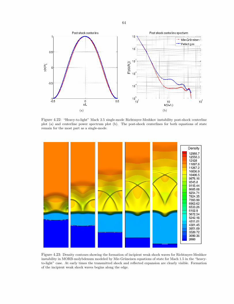
55
(a) (b)
Figure 4.12: “Light-to-heavy” Mach 2.5 single-mode Richtmyer-Meshkov instability post-shock centerlineplot (a) and centerline power spectrum plot (b). The post-shock centerlines for both equations of stateremain for the most part as a single-mode.
4.5 “Light-to-heavy” triple-mode
When multiple modes are present, products of variables in the Euler equations can lead to nonlinear
reinforcement or interference across modes when two wave numbers sum to a third. One case of
triple-mode Richtmyer-Meshkov instability with the mode coupling k1 = k2 + k3 where k2 = 23k1,
k3 = 13k1, and k1h1 = k2h2 = k3h3 is now examined. As a starting point the wavenumbers from
the previous single-mode investigation for k1 are retained, but with a corrugation amplitude that
is 2% of the wavelength. Tabulation of the three initial wavelengths and associated amplitudes are
given in table 4.6 for MORB-molybdenum and perfect gas simulations. Figure 4.13 shows density
MORB-molybdenumMs k1h1 k2/k1 k3/k1
2.5 0.04π 2/3 1/3Perfect gas
Ms k1h1 k2/k1 k3/k1
1.87 0.025π 2/3 1/3
Table 4.6: Initial conditions for triple-mode Richtmyer-Meshkov instability in the “light-to-heavy”case for Mie-Gruneisen and perfect gas equations of state
gradient magnitude contours for the present triple-mode case and matched perfect gas. Again, the
amplitude of the mixing layer for the perfect gas cases is seen to lag behind that of the corresponding
MORB-molybdenum cases. Consequently roll-up is delayed in time as well.
56
(a)
(b)
(c)
Figure 4.13: “Light-to-heavy” MORB-molybdenum Mach 2.5 triple-mode Richtmyer-Meshkov instabilityschlieren plots and equivalent perfect gas plots for nondimensional times 5.31, 10.6, and 15.9
57
4.5.1 Amplitude and growth rate
The mixing layer amplitude and growth rate are given in Figure 4.14. A variation in start-up time
of the same order of magnitude as in the single-mode case is again observed. A similar order of
magnitude variation in growth rate oscillations is also observed. However, three distinct oscillation
frequencies are now observed, associated with the three different wavelengths of the corrugation.
Tabulation of frequency values is given in table 4.7. Strong correlation is observed between the
observed oscillation frequencies and predicted values from the associated zero-corrugation problem.
(a) (b)
Figure 4.14: “Light-to-heavy” Mach 2.5 triple-mode Richtmyer-Meshkov instability amplitude growth plot(a) and amplitude growth rate plot (b). A start-up time difference is clearly observable between the MORB-molybdenum and perfect gas case. Post-start-up oscillations in growth rate for MORB-molybdenum are atmuch greater frequency and amplitudes than those of the perfect gas.
Table 4.7: Dominant growth rate oscillation frequencies f2Dτ for “light-to-heavy” triple-modeRichtmyer-Meshkov instability and approximate perturbed transmitted and reflected shock oscil-lation frequency, fT1Dτ and fR1Dτ , respectively, based on solution to the zero-corrugation Riemannproblem
58
4.6 “Heavy-to-light” single-mode
Presently the single-mode “heavy-to-light” case is investigated. Again MORB and molybdenum are
used for the materials with Mie-Gruneisen equation of state and air and SF6 as a starting point for
perfect gases. Mach numbers of 1.5 and 2.5 for the MORB and molybdenum case provide the basis
for comparison in parameter space for the “heavy-to-light” case as well. For the Mach 1.5 case a
5% of the wavelenth initial corrugation amplitude was taken as well. For the Mach 2.5 case, due
to the large compression of the corresponding perfect gas case interface by the shock that would
result, a smaller amplitude of 2% of the wavelenth was taken. Tabulation of these initial conditions
and relevant post-shock quantites for zero-corrugation are found in Table 4.8. Again, the unshocked
prefect gases are taken to be at approximately room temperature and pressure (T=300 K, p=1
atm). Likewise, the unshocked Mie-Gruneisen fluids are in thermodynamic equilibrium at (ρ0, p0),
repsectively. The entries for MORB and molybdenum are tabulated below, including initial and
post-shock conditions as well as properties for the corresponding matched perfect gas cases. Figure
Table 4.8: Initial conditions for single-mode Richtmyer-Meshkov instability in the “heavy-to-light”case for Mie-Gruneisen and perfect gas equations of state
Table 4.9: Perfect gas properties for single-mode Richtmyer-Meshkov instability in the “heavy-to-light” case
4.15 (a) shows density gradient magnitude contours for the Mach 1.5 case and matched perfect gas
respectively. Figure 4.15 (b) shows density gradient magnitude contours for the Mach 2.5 case and
matched perfect gas. A greater deal of variation in shape is observed from one case to another for
the “heavy-to-light” cases, particularly at the higher Mach number, which demonstrates a wider
spike.
59
(a) (b)
(c) (d)
Figure 4.15: “Heavy-to-light” MORB-molybdenum (left) and equivalent perfect gas (right) single-modeRichtmyer-Meshkov instability schlieren plot comparison for Mach 1.5 incident shock at nondimensionaltimes (a) 3.01, (b) 6.02, (c) 9.02, and (d) 15.04
(a) (b)
(c) (d)
Figure 4.16: “Heavy-to-light” MORB-molybdenum (left) and equivalent perfect gas (right) single-modeRichtmyer-Meshkov instability schlieren plot comparison for Mach 2.5 incident shock at nondimensionaltimes (a) 7.9, (b) 23.71, (c) 31.41, and (d) 47.22
60
4.6.1 Amplitude and growth rate
Figures 4.5 and 4.5 display nondimensionalized results for Mach 1.5 and 2.5 Richtmyer-Meshkov
instability respectively for the MORB-molybdenum “heavy-to-light” case and associated perfect gas
matching. The growth rate plots have been scaled by the alternative prediction [54],
h∞ =12
(h−0 + h+0 )kA+∆v, (4.26)
which gives better agreement. Unlike the “light-to-heavy” case, a much higher degree of similarity is
observed in the features of the growth plots. The most notable difference is that the peak growth rate
attained by the perfect gases is considerably less than those of the MORB-molybdenum. Start-up
time and growth rate oscillations are all similar in magnitude. Evidently the wavenumber required
to yield a matching of growth rate correlates directly to wave speed for the present case. Again,
the linear growth regime is not distinctly evident in the present growth rate plots. Just as in the
“light-to-heavy” case, the decay in growth rate deviates between equations of state more as the
strength of the shock increases, MORB-molybdenum demonstrating a higher decay rate. This is
in part due to the larger compression of the perfect gas interface requiring a bigger h−0 to obtain
similar h+0 k values, thus yielding a larger linear growth rate for the perfect gas by the prediction of
equation (4.26).
MORB-molybdenumMs τfT1D τf2D
1.5 1.21 1.212.5 1.20 0.49
Perfect gasMs τfT1D τf2D
1.244 1.26 1.221.934 0.42 0.38
Table 4.10: Growth rate oscillation frequency f2D for “heavy-to-light” Richtmyer-Meshkov instabilityand approximate perturbed transmitted shock oscillation frequency fT1D based on solution to thezero-corrugation Riemann problem
4.6.2 Integral vorticity
Examination of the vorticity distribution for the “heavy-to-light” case shortly after shock-contact
interaction is now presented. Figures 4.19 and 4.20 display normalized vorticity distributions and
associated power spectrum shortly after shock interaction for MORB-molybdenum Mach 1.5 and
2.5 Richtmyer-Meshkov instability and corresponding perfect gas cases of matched initial conditions
respectively. Just as in the “light-to-heavy” case, the vorticity distribution exhibits the behavior of
a sinusoidal distribution with a single-mode to within roughly 15%.
61
(a) (b)
Figure 4.17: “Heavy-to-light” Mach 1.5 single-mode Richtmyer-Meshkov instability amplitude growth plot(a) and amplitude growth rate plot (b). The plots show a greater level of similarity than the “light-to-heavy”case. Start-up times are observed to be on the same order of magnitude. Post-start-up oscillations in growthrate also demonstrate similar frequencies and amplitudes.
(a) (b)
Figure 4.18: “Heavy-to-light” Mach 2.5 single-mode Richtmyer-Meshkov instability amplitude growth plot(a) and amplitude growth rate plot (b). Again, start-up times are observed to be on the same order ofmagnitude. Post-start-up oscillations in growth rate also demonstrate similar frequencies and amplitudes.
62
(a) (b)
Figure 4.19: “Heavy-to-light” Mach 1.5 single-mode Richtmyer-Meshkov instability post-shock integralvorticity plot (a) and integral vorticity power spectrum plot (b). Significant change is observed betweenequations of state due to the nature of the Hugoniot.
(a) (b)
Figure 4.20: “Heavy-to-light” Mach 2.5 single-mode Richtmyer-Meshkov instability post-shock integralvorticity plot (a) and integral vorticity power spectrum plot (b). Significant change is observed betweenequations of state due to the nature of the Hugoniot
63
4.6.3 Post-shock centerline
Examination of the centerlines for the “heavy-to-light” case post-shock yields similar results to
the “light-to-heavy” case. Figures 4.21 and 4.22 display normalized centerline plots and associ-
ated power spectrum shortly after shock interaction for MORB-molybdenum Mach 1.5 and 2.5
Richtmyer-Meshkov instability and corresponding perfect gas cases of matched initial conditions.
The centerlines remain as a single-mode to within roughly 5%.
(a) (b)
Figure 4.21: “Heavy-to-light” Mach 1.5 single-mode Richtmyer-Meshkov instability post-shock centerlineplot (a) and centerline power spectrum plot (b). Slight variation in shape occurs, however, the post-shockcenterlines for both equations of state remain for the most part as a single-mode.
4.6.4 Incipient weak shock waves
Figure 4.23 gives density contour plots at several different times for “heavy-to-light” Mach 1.5
Richtmyer-Meshkov instability in MORB-molybdenum. Clearly evident in the contour plots is a
transmitted shock and reflected expansion wave. However, an additional and somewhat unexpected
series of shock waves is observed to form within the region of the expansion fan. These shock waves
first form along the boundary and propagate away from the corrugation. A somewhat analogous
phenomenon has been observed in Rayleigh-Taylor instability [61]. For Rayleigh-Taylor instability,
Olson and Cook observed that the acceleration of an interface driven by a constant gravitational
field generated shocklets, much in the same way a piston does, which eventually catch up to one
another to form a weak shock. Presently, in “heavy-to-light” Richtmyer-Meshkov instability, the
formation of incipient weak shock waves generated by oscillations in the difuse material contact are
observed. It is evident that waves produced by the perturbed transmitted shock cause oscillations
64
(a) (b)
Figure 4.22: “Heavy-to-light” Mach 2.5 single-mode Richtmyer-Meshkov instability post-shock centerlineplot (a) and centerline power spectrum plot (b). The post-shock centerlines for both equations of stateremain for the most part as a single-mode.
Figure 4.23: Density contours showing the formation of incipient weak shock waves for Richtmyer-Meshkovinstability in MORB-molybdenum modeled by Mie-Gruneisen equations of state for Mach 1.5 in the “heavy-to-light” case. At early times the transmitted shock and reflected expansion are clearly visible. Formationof the incipient weak shock waves begins along the edge.
65
Figure 4.24: Density contours showing the formation of incipient weak shock waves for Richtmyer-Meshkovinstability in fluids with perfect gas equations of state for Mach 1.244 in the “heavy-to-light” case. At earlytimes the transmitted shock and reflected expansion are clearly visible. Formation of the incipient weakshock waves begins along the edge.
66
in the shape of the interface centerline. In the present case of “heavy-to-light” Ricthmyer-Meshkov
instability the strength of these oscillations is strong enough to generate noticeably strong shocks
within the heavy material for both Mach 1.5 and 2.5 cases. A similar set of incipient weak shock
waves is observable for the corresponding perfect gas cases, as seen in Figure 4.24 for a 5% intial
corrugation amplitude. The formation of several incipient weak shock waves is clearly observable.
67
Chapter 5
Level-set, ghost cell methodology
In the following sections an Eulerian, Cartesian mesh, ghost fluid methodology is developed for
single-phase impact-driven flows with free surfaces. The methodology utilizes a level-set to define
the location of the material-vacuum interface. Ghost cells are interpolated based on surface normal
Riemann problems along gradient trajectories of the signed distance function [8, 83]. Flux recon-
struction along each Cartesian direction of the domain is achieved by subdividing in a way that
allows for robust treatment of grid-scale sized voids. Additionally, introduced is a two-variable ap-
proach to the reinitialization of the distance function from the level-set which leaves the material
boundary defining zero level-set essentially intact. Implementation of the code in parallel with adap-
tive mesh refinement (AMR) is performed in California Institute of Technology’s VTF (Virtual Test
Facility) AMROC [15–17]. Results for several impact-driven flows in vacuum of interest are given
in one and two dimensions to demonstrate the methodology for fluids with Mie-Gruneisen equation
of state. First, in one dimension an impact problem involving two finite length aluminum slabs is
examined. Next, a similar three-dimensional axisymmetric impact problem involving aluminum rods
is demonstrated. Lastly, the axisymmetric impact of a sphere and plate is examined.
5.1 Level-set
level-sets provide a simple way to define an arbitrarily complex surface by a scalar in an Eulerian
setting. The level-set scalar is evolved by the linear advection equation
∂φ
∂t+ ~u · ~∇φ = 0, (5.1)
allowing for the natural splitting of isocontours which can be utilized to define material regions.
Presently, for the purpose of simulating flows with fluid-vacuum interfaces, fluid and vacuum regions
68
of a single-phase flow are defined by a scalar φ, where
φ < 0, vacuum, (5.2)
φ = 0, interface, (5.3)
φ > 0, material. (5.4)
The advection of the zero level-set is therefore of critical importance to such a level-set method.
Figure 5.1: Schematic of level-set definition for fluid-vacuum interface problems
5.1.1 Ghost cells
The assignment of ghost cell values in a narrow band outside of a free surface should at a minimum
provide an approximation to the proper traction conditions. It was initially proposed by Fedkiw
[22] that the signed distance function should be utilized to apply the proper traction conditions
at an interface between two materials. For a given fluid region defined by a level-set the entropy
and velocity field are extrapolated along tangent curves of the signed distance function. The final
conservative ghost fluid vector of state is given by enforcing the pressure of the contacted material.
The method was initially applied to ideal gas law fluids. For a general fluid, such as those defined
by Mie-Gruneisen equation of state, or even a solid, it is not in general useful to extrapolate entropy
which may not be simply extracted. Instead it is more practical to utilize approximate Riemann
problem solutions [7, 8], analogous to using an isentrope which is an approximate solution Riemann
69
problem solution to third-order in entropy [85]. For each ghost cell, as in Figure 5.2, a tangent path
to the signed distance function is traced out to the location of the free surface,
~xs = ~xi,j +∫ 0
φi,j
~n(s)ds, (5.5)
where
~n(s) =~∇φ‖~∇φ‖
. (5.6)
Figure 5.2: Schematic of a ghost cell band and its tangent path to a free surface
Numerically this path integration is carried out by an adaptive stepping third-order Runge-Kutta
integration with the bilinear interpolation of the gradient of φ. The differential step ds is taken to
be
ds = min(3∆x/4,max(|φ|,∆x/10)), (5.7)
with integration complete upon reaching a value of φ greater than zero. Once the surface is reached
an interpolation of the conserved vector of state is performed by weighted bilinear interpolation to
give an approximation to the state locally. The surface normal, defined by the gradient in the signed
distance function, is then utilized to decompose the momentum state into a local coordinate system
for determining a Riemann problem solution. This Riemann problem solution is then assigned to
the ghost cell.
70
5.1.1.1 Riemann solver
For most fluids the solution to the Riemann problem between left and right states is comprised
of compressive shock wave discontinuities, isentropic expansion waves, and contact discontinuities
[47, 85]. A valid solution must yield a common pressure and velocity across the shock and expansion
waves connecting left and right states. The locus of states accessible by expansion or compression
is known as a Hugoniot. It is useful to think of this Hugoniot in terms of velocity and pressure in
order to meet the matching constraint from left and right states. Figure 5.3(a) depicts left and right
state velocity-pressure Hugoniot with intersection defining the appropriate solution. The related
Riemann problem solution wave diagram in space and time is shown in Figure 5.3(b) composed of
leftward traversing shock and contact discontinuity and rightward expansion wave.
(a) (b)
Figure 5.3: Schematic of a Riemann problem solution consisting of shock and expansion waves
Analytically the shock branch of the Hugoniot of states can be described by a transcendental
equation derived from Rankine-Hugoniot jump conditions,
ecd = eR/L
+12
(pcd + pR/L
)(1/ρcd − 1/ρR/L
), (5.8)
and
ucd = uR/L±√
(pcd − pR/L)(1/ρR/L− 1/ρcd). (5.9)
Alternatively, the expansion branch of the Hugoniot is described by integral equations
ucd = uR/L±∫ pcd
pR/L
1ρcdp′, (5.10)
71
and
ρcd = ρR/L
+∫ pcd
pR/L
1cdp′. (5.11)
For most fluid equations of state no analytic solution to the Riemann problem is attainable.
Solution must therefore be performed numerically by root finding for the intersection of the Hugoniot.
Additionally, it may be necessary to use root finding to produce the shock-branch and integration
quadrature for the expansion-branch of each Hugoniot. Solving the Riemann problem can therefore
be a relatively expensive computational procedure. Fortunately for a Godunov-style numerical
solver applied to many flows of interest, it is in general unnecessary to solve the Riemann problem
to numerical precision to approximate fluxes at midpoints.
5.1.1.2 Linearized Riemann solver
A variety of simple low-order approximations to Riemann problem solutions have proven to be, for
many flows of interest, a practical alternative to full solutions for Godunov solvers [13, 45, 46, 72,
86, 87]. Presently, two approaches are used for approximating the Riemann problem solution. The
first is a simple linear p− u approximation to the Hugoniot introduced by Colella [13],
pcd = pL/R± ρ
L/RaL/R
(ucd − uL/R). (5.12)
From this simple linear Hugoniot approximation can be obtained an expression for ucd and pcd
strictly in terms of left and right state quantities,
ucd =ρRuRaR
+ ρLuLaL
ρRaR
+ ρLaL
. (5.13)
Density along the Hugoniot can be approximated by the linear equation
ρcd = ρL/R
+ (pcd − pL/R)/a2L/R
. (5.14)
This simple solver is relatively robust for moderate shock strengths and is applied to the first two
test problems examined. Such an approximation can be considered as a single step of a Newton-
Raphson root finding approximation to the Hugoniot intersection problem. It is noteworthy that
for problems involving a free surface the value of pcd = 0 is a given. This reduces the computational
cost of solving the full Riemann problem by more than half that of a two-material problem where
pcd is an unknown. For the vacuum case when pL/R
> 0 it is then only necessary to perform a simple
numerical integration of equations (5.10) and (5.11). Again, in practice it is not necessary to have a
solution to numerical precision. Instead, a limited number of integration steps can be utilized to give
a higher-order approximation, useful for stronger expansions. Similarly, for cases with pL/R
< 0 a
72
higher-order approximation to the Riemann problem solution can be obtained by applying a limited
number of root finding steps. Utilizing Secant root finding and third-order Runge-Kutta integration,
this higher-order approach is applied to the third test problem examined of a sphere-plate impact.
5.1.2 Level-set reinitialization
The use of a the signed distance function to define ghost cells in the previous section presents an
additional complication. In general the level-set does not carry any additional meaning besides
defining regions by a sign change. However, since the signed distance function is utilized in defining
ghost cells it becomes natural to use the level-set scalar to carry this information. Unfortunately the
linear advection equation does not constrain the level-set scalar to satisfy the Eikonal equation for all
time as a signed distance function should. It is therefore an important part of level-set methods to
periodically reinitialize the level-set into a true distance function which satisfies the Eikonal equation
[26, 64, 75, 83],
‖−→∇φ‖ = 1. (5.15)
Presently, to achieve a level-set which satisfies the above constraint, a modified version of the artificial
time marching differential equation based reinitialization of Russo and Smereka [75] is introduced.
Sussman [83] first introduced the concept of differential equation based reinitialization, utilizing the
Hamilton-Jacobi differential equation
∂φ
∂τ+ S(φ0)(‖
−→∇φ‖ − 1) = 0 (5.16)
which tends to the unique viscosity solution of the Eikonal equation as τ approaches infinity. For
numerical purposes S(φ0) is a smoothed out sign function of the initial condition defined by
S(φ0) =φ0
φ20 + ε2
(5.17)
with ε given by the grid length scale. For a first-order continuous zero level-set, reinitialization
numerically by this approach directly can yield a shift of the location of the zero level-set on the
order of the grid length scale. Furthermore, at corners in the zero level-set the location is significantly
rounded and shifted. For situations where the level-set is advected only a fraction of the grid length
scale over long periods of time the approach is therefore inadequate when applied repeatedly. A
good numerical reinitialization should shift the location of the zero level-set by as little as possible.
Russo [75] introduced a modified version of the approach which used a one-sided direct calculation
of distance for points near the level-set. Hartmann et al. [26] introduced a more sophisticated
numerical approach to constrain the location of the zero level-set.
Presently, a modified version of the work in [75] is introduced. The current method utilizes a two-
73
variable approach. The first variable, denoted here by ψ, is never reinitialized and initially contains
the same zero level-set as the distance function but is an otherwise meaningless scalar advected by
the physical flow field,∂ψ
∂t+ ~u · ~∇ψ = 0. (5.18)
The second variable, denoted here by φ, is the level-set which is advected physically by equation
(5.18) as well, but is reinitialized periodically to the distance function by solution to differential
equation in artificial time τ . The function ψ is utilized to tie down the zero level-set for the
numerical method. The numerical approach is defined as follows:
Here Γ is used to denote points nearest to the zero level-set that are positive in value of ψ. Applying
the the direct distance calculation to only one side of the interface alleviates over constraining which
may lead to inconsistencies. The value di,j is given by a direct approximation to the distance of
such points,
di,j =ψi,j
‖~∇ψi,j‖. (5.20)
Evaluation of ‖~∇ψi,j‖ numerically requires special consideration. At smooth first-order continuous
features in the level-set contour a high-order approximation is desirable. Alternatively, at corners
and cusps a low-order approximation is best. Therefore the approximation of ‖~∇ψi,j‖ is taken as
the maximum of the central slope limiter of Van Leer [88] and
|ψi+l,j+k − ψi,j |√(l∆x)2 + (k∆y)2
, ∀ l, k = −1, 0, 1 with ψi+l,j+kψi,j ≤ 0. (5.21)
Evaluation of ‖~∇φi,j‖ is performed by the methods described in [63] using a fifth-order WENO
scheme [37, 48] with third-order Runge-Kutta temporal discretization.
To demonstrate reinitialization of a meaningless scalar field by the means discussed, consider the
initial profile
φ(τ = 0, x, y) = C tanh(δ(r − r0)), (5.22)
which has the zero isocontour of a circle of radius r0 (see Figure 5.4), but is not the signed distance
function for a circle. Figure 5.5 shows the artificial time reinitialization solution after 40, 80, 120,
160, 200, and 240 numerical steps for a uniform mesh of 200x200 points with a CFL of 0.5 on a
periodic domain. Initially the scalar values in the flattest regions are rapidly forced away from their
true signed distance values. After 240 steps the solution appears to have reached it steady state and
resembles the expected cone-shaped solution for the signed distance function of a circle.
74
Figure 5.4: Initial conditions utilized for the reinitialization of the distance function for a circle from ameaningless scalar through numerical solution to differential equation for a mesh size is 200x200 points
For practical application to the ghost fluid method it is only necessary to reinitialize points in-
side of a narrow band around a material interface. For example, for three-dimensional axisymmetric
simulation of a sphere-plate impact Figure 5.6 shows the narrow region around the impact reini-
tialized to the distance function. It is important that the scalar ψ remain continuous to achieve a
good approximation to the zero level-set distance. To force ψ to remain continuous an artificial time
reinitialization is applied,
∂ψ
∂τ+ S(ψ)
(max
(∣∣∣∂ψ∂x
∣∣∣, ∣∣∣∂ψ∂y
∣∣∣)− 1)
= 0, (5.23)
for a few points outside of the band of ghost cells utilized.
5.2 Numerical method
The ghost fluid methodology is composed of two separate essential components. The first is the pre-
viously discussed management of the reinitialization of the level-set into a signed distance function.
This function is performed after a fixed number of advances in real time of the solution for a finite
number of iterations in artificial time. The second component is the physical solver which advances
the flow in time. Each advance in time of the solution, performed by third-order Runge-Kutta TVD
temporal discretization, is essentially composed of two steps. Firstly, the signed distance function
is utilized to interpolate ghost cells from surface normal Riemann problem solutions. Secondly,
75
Figure 5.5: Reinitialization of the distance function for a circle from a meaningless scalar through numericalsolution to differential equation for a mesh size is 200x200 points. After roughly 240 steps in artificial timethe steady-state solution to the Eikonal equation is achieved.
76
(a) (b)
Figure 5.6: Reinitialization band around fluid-vacuum interface for a sphere-plate impact problem. Initiallythe level-set is assigned to be the true distance function. Later only a narrow band around the fluid-vacuuminterface is maintained as a signed distance.
a reconstruction of fluxes at midpoints must be performed to update each physical cell. Special
treatment of near vacuum-fluid interfaces is required to ensure that no waves propagate through the
vacuum to a neighboring free surface. The following section describes how this can be achieved in a
simple robust manner.
5.2.1 Domain decomposition
The standard reconstruction of midpoint fluxes along a given direction is inadequate for situations
where gradients in the level-set are discontinuous. For such situations neighboring ghost cells will
have diverging paths along the tangent to the gradient of the level-set and thus refer to points on
the zero level-set that are unrelated in position and state. Such situations are fundamental to the
impact of two material regions in a vacuum when described by a single levelest. Before contact no
mechanical information must be transmitted between regions separated by even a single cell. To
properly handle such situations the domain is subdivided accordingly. Treatment of ghost cell and
material regions is done separately. For each subdivided material region fluxes at the fluid-vacuum
contact are determined by approximation of the solution to a Riemann problem in terms of the
surface normal. Interior fluid midpoint point fluxes are determined by padding the region on either
side with the solution to the Riemann problem and then performing a local Lax-Fredrichs splitting
of fluxes,
f± =12(f(q(x))± |λmax|q(x)
), (5.24)
77
in conjunction with fifth-order WENO to reconstruction. Ghost cells are subdivided into regions
defined by the sign of the level-set gradient along the direction. Again for the ghost cells nearest
to the contact flux reconstruction is determined by Riemann problem. The ghost cell regions are
truncated to only include points within three cells of a material point. Figure 5.7 depicts the presently
used subdivision for a situation in which a material region has a hole in it. Reconstruction of fluxes
in the horizontal direction for the cells highlighted in red requires six subdivisions. It is important
to note that each region may contain an overlap in the midpoints utilized for flux reconstruction. A
single flux associated with a given midpoint is not possible and the scheme is not conservative.
5.2.2 Adaptive mesh refinement
As a simple extension to an adaptive mesh refinement capable solver each mesh patch is treated
in the same manner. In taking this approach potential complications can occur when small voids
or thin ligaments on a fine mesh are prolonged onto a coarse mesh. It is particularly problematic
near thin ligaments where ghost cells would be identified but tracing along the tangent to the signed
distance function would not result in actually reaching a free surface for use in a Riemann solver. To
avoid such complications ghost cells that are within the appropriate limited band but do not result
in a proper interpolation are flagged to be ignored.
Proper mesh refinement criteria for a level-set should include a curvature-based detection. Presently,
a much simpler technique is utilized by flagging about changes in sign of the level-set φ. Additionally,
density and velocity tolerance flagging criteria are applied. Vacuum cells are more or less inactive
cells, except those nearest to free surfaces. It is therefore possible to use a very coarse base mesh
with a large factor of refinement to the next mesh. For instance, for the axisymmetric simulation of
a sphere-plate impact problem (see Figure 5.8) one level of refinement is used with a base mesh of
64x64 and refinement factor of 16x resulting in an equivalent mesh of 1024x1024 points.
5.3 Test problems
5.3.1 One-dimensional aluminum impact problem
To first explore the ghost fluid method outlined in previous sections for impact-driven flows in one
dimension a unigrid code was developed in MATLAB. As a simple test an impact problem is utilized
which demonstrates the capability of the method to handle single-cell voids in one dimension. Signed
distance function reinitialization is performed directly rather than by partial differential equation
solution. Additionally, a simple cell erosion approach to handling spallation is implemented in this
one-dimensional code. When tension above some modeled value is achieved at a corresponding point
that point is replaced by a vacuum. A grid scale violation of conservation occurs from the erosion
78
(a)
(b)
Figure 5.7: Schematic of the coordinate-wise decomposition of the domain for midpoint flux reconstructionbased on the distance function. Regions i, iii, iv, and vi are ghost cells separated based on the gradient ofthe signed distance function. Regions ii and v are physical material regions. At each of the boundaries ofthe regions a Riemann problem for the surface normal direction is used to approximate the flux and pad theregions. For all other midpoints a fifth-order flux-splitting WENO reconstruction of the flux is utilized.
79
(a) (b)
Figure 5.8: Adaptive mesh refinement for ghost fluid method axisymmetric simulation of a sphere-plateimpact. One level of refinement is utilized to solve the problem. The base mesh is very coarse at only 64x64while the fine mesh is 16x refinement of the base.
and the approach is not a practical solution to modeling spallation in many situations, particularly
those in more complex multidimensional problems.
The initial conditions for the impact problem are plotted in Figure 5.9. Two aluminum slabs of
finite length 0.07 m, modeled by Mie-Gruneisen equation of state, initially are separated on either
sides of the origin by 0.02m. The slabs travel in opposite directions at a speed of 400 m/s until they
meet at the origin and are welded into one by impact. The domain is discretized by 200 uniform
points and adaptive time stepping is utilized to maintain a CFL of 0.75 throughout the simulation.
Upon impact two shock waves travel in opposite directions away from the impact, shown in Figure
5.10. The shock waves travel until reaching the ends of the slab and generate a reflected expansion
waves traveling towards the origin (see Figure 5.11). Upon reaching the origin a large amount of
tension is created which splits the single slab of aluminum back into two. Figure 5.12 shows the
resulting split slab with a shockwave closely followed by an expansion wave as a result of the split.
The collision is effectively inelastic with the resulting velocity profiles in the individual slabs slightly
less in magnitude on average than the initial 400 m/s.
5.3.2 Three-dimensional axisymmetric rod impact problem
As a second test problem, analogous to the first impact problem studied in one dimension, next
simulated is the three-dimensional axisymmetric impact of two aluminum rods. Signed distance
function reinitialization is performed by partial differential equation solution and no simple cell ero-
sion approach to handling spallation is implemented. The two rods are initially in contact traveling
at 500 m/s in opposite directions. The two rods have length 0.04 m and radius of 0.01 m. A base
mesh of 64x128 points with 3 levels of 2x refinement was used to simulate the impact with adaptively
80
Figure 5.9: Plot of the initial conditions for a one-dimensional simulated impact of two finite aluminumpieces modeled by Mie-Gruneisen equation of state traveling in opposite directions at 400 m/s. The domainis decomposed in to 200 points including the void regions.
81
Figure 5.10: One-dimensional finite length 400 m/s Mie-Gruneisen aluminum impact problem solution att = 18.0 µs. Shock waves are seen to propagate away from the impact on either side.
82
Figure 5.11: One-dimensional finite length 400 m/s Mie-Gruneisen aluminum impact problem solution att = 30.0 µs. Once the shock waves reach the end of the finite length material a reflected expansion wave isgenerated as is presently shown.
83
Figure 5.12: One-dimensional finite length 400 m/s Mie-Gruneisen aluminum impact problem solutionat t = 42.0 µs. Once the expansion waves meet at the middle of the material a large amount of tensionoccurs splitting the material in two again. Each piece propagates away at an average speed slightly less inmagnitude than the original impact speed.
84
maintained CFL of 0.75. Figure 5.13(a) shows density contours shortly after impact at time 1.25
micro seconds. Two planar shocks are immediately created as in the one-dimensional problem, but
due to the free surface of the cylinder the initial compressive stress of the impact cannot be sup-
ported and the rod begins to expand in the radial direction behind the shock front. The expanding
material creates tension behind the increasingly weak shockwave. The expansion waves generated in
the radial direction eventually meet and generate compression, seen at time 6.25 in Figure 5.13(b).
The now weak shock reflects off the end of the rods. A series of complex wave patterns develops due
to radial and horizontal waves bouncing between free surfaces.
5.3.2.1 Three-dimensional axisymmetric sphere-plate impact problem
To further examine the ghost fluid method for free surface impact problems a three-dimensional
axisymmetric aluminum sphere-plate impact problem is simulated. The sphere has a radius 0.025 m
and travels toward the plate at 500 m/s. The plate has a thickness of 0.01 m. A base mesh of 64x64
points is utilized with 1 level of 16x refinement for an equivalent of 128 points across the diameter
of the sphere. A CFL of 0.75 was adaptively maintained throughout the simulation.
Density and x-velocity component contours are given in Figure 5.14 for initial conditions and two
successive times. The sphere generates a continuous series of impacts as more and more of it welds
to the plate. These impacts set up a curved shock which reflects off the back end of the plate and
generates tension. Failure to support the compression of the impact at the free surface of the plate
forces expansion. The expansion sets up something analogous to a “splash” as the material tries to
move aside and is forced in the direction of least resistance. By 3.0 micro seconds a very complex
and seemingly chaotic set of waves reflecting through the medium are observed. Further away from
the impact site the x-velocity component remains close to the initial 500 m/s in magnitude. The
feature analogous to a “splash” continues to grow, perhaps unrealistically due to poor numerical
treatment at regions of high curvature in the free surface.
One quantity of physical interest for such impact problems is the hole size generated. The ability
to accurately capture the impact hole diameter is essential for any simulation to be a practical
tool for prediction. Hole radius results for the present ghost fluid method and material model are
presented in Figure 5.16. The growth rate of the impact hole is observed to only gradually decrease
with time, perhaps never to reach a constant value. The simulation therefore does not provide a
realistic prediction, as should be expected without shear strength.
85
(a)
(b)
(c)
Figure 5.13: Axisymmetric simulation of the collision of two aluminum rods initially traveling 500 m/s inopposite directions in a vacuum. Density contours shown at times 1.25, 6.25, and 11.25 micro seconds.
86
(a) (b)
(c) (d)
(e) (f)
Figure 5.14: Axisymmetric simulation of a sphere impacting a plate at 1.0 km/s. Density and x-velocitycomponent contours shown at time 0.0, 3.0, and 6.0 µs.
87
(a) (b)
(c) (d)
(e) (f)
Figure 5.15: Further results for axisymmetric simulation of a sphere impacting a plate at 1.0 km/s. Densityand x-velocity component contours shown at time 9.0, 11.0, and 13.0 µs.
88
(a) (b)
Figure 5.16: Aluminum 1.0 km/s sphere-plate impact hole radius as a function of time. The hole radius isseen to increase as a function of time, only slowing gradually.
89
Chapter 6
Nonlinear elastic-plastic solids
In the following Chapter a brief investigation of the assumptions made in using an isotropic stress
model for solids is undertaken. Solids are distinguishable from fluids in that they resist continuous
deformation under shear stresses. It is therefore reasonable to expect that isotropic models will not
give realistic results when shear is important. Furthermore, most solids can support anisotropic
states of stress in a limited capacity. For many ductile solids under high compressive stress plastic
yielding occurs limiting the amount of shear stress and thus anisotropy in the stress state [31, 96].
Under such conditions at least some similarity in flow structure should be expected between purely
fluid and solid material models. In the following sections these issues are explored using comparisons
between materials with Mie-Gruneisen equation of state and hyper-elastic solid models.
6.1 Nonlinear hyper-elastic solids
At a minimum, to simulate the response of a material to internal and external forces by continuum,
a model that relates relative displacement of points to internal stresses must be made. The dis-
placement of points can be described as a function of the initial position X and the present time t,
x = x(X, t). The relative displacement of two infinitesimally close points is then described by the
deformation gradient tensor [5, 78],
Fij =∂xi∂Xj
. (6.1)
For isotropic inviscid fluids only volumetric changes are of interest in relation to density changes,
related to the deformation gradient tensor by
ρ0/ρ = det(F). (6.2)
Alternatively, for a solid the stress state may be anisotropic and depend on the full nature of
the deformation. Material models which relate stress strictly to the deformation gradient tensor
and some other thermodynamic quantity are known as hyper-elastic solid models [28, 55, 56]. For
90
consistency it is convenient to formulate the hyper-elastic solid model directly in terms of internal
energy
e = e(X,F, s), (6.3)
where s is the entropy. The definition of the stress tensor follows directly from required consistency
in conservation of energy [78],
σij = −ρ ∂e
∂FikFjk. (6.4)
An alternative equivalent formulation of a hyper-elastic solid is in terms of the inverse deformation
gradient tensor defined by f = F−1. In terms of the inverse deformation gradient tensor the stress
tensor becomes
σij = −ρ ∂e
∂fkjfki. (6.5)
Further consideration of frame indifference arguments demonstrate that internal energy must only
be a function of C = FT
F, the right Cauchy-Green tensor [78].
e = e(X,C, s) (6.6)
Additionally, only isotropic materials are considered. For isotropic solids the internal energy must
depend on the right Cauchy-Green tensor only through its invariants [78],
I1 = tr(C),
I2 = det(C)tr(C−1) = 12
[tr(C2)− tr(C)2
],
I3 = det(C).
(6.7)
6.1.0.2 A simple hyper-elastic aluminum model
A large variety of models for equations of state for various materials can be found in literature
[28, 55, 56]. Presently, a simple hyper-elastic model is used that was proposed by Miller and Colella
[55] that is a variant of the Blatz and Ko model,
e =µ0
2ρ0
(I1 − 3I1/3
3
)+∫ ρ0
ρ
p(ρ′, s)ρ′2
dρ′. (6.8)
Here p(ρ, s) could come from a variety of models for the bulk response including Hugoniots. Cur-
proposed in [55] is used. For aluminum the coefficients to this polynomial are taken as w1 = 72.0
GPa, w2 = 172.0 GPa, and w3 = 40.0 GPa. Additionally, the shear modulus for aluminum is taken
91
to be µ0 = 24.8 GPa and ρ0 = 2785.0 kg/m3. The model is strictly dependent on the deformation
of the material as no thermodynamic quantities other than density are utilized. The stress tensor
associated with this equation of state is then [28]
σ = µ0
ρ
ρ0
(FF
T
−( ρρ0
)−2/3
I)
+ p(ρ, s)I. (6.10)
Furthermore, for flux-splitting and CFL calculations it is useful to have acoustic propagator tensor.
For direction n the acoustic propagator tensor is given by
Anij = −1
ρ
∂σin
∂fknfkj (6.11)
with no sum on n [28]. For the modified Blatz and Ko model the acoustic propagator tensor in
analytic form is therefore
Anij =
µ0
ρ0
FnkFnkδij +(∂p(ρ)
∂ρ+
13µ0
ρ0
( ρρ0
)−2/3)δinδjn (6.12)
6.1.1 Plasticity
Most ductile metals can only support a limited amount of anisotropic stress before yielding occurs.
Upon yielding an irreversible change in the material occurs resulting in what is observed as plastic
deformation. For ductile metals the process of yielding is caused by dislocation motion in the
atomic crystal structure [31]. For metals where the crystal grains are randomly oriented and grain
sizes are much smaller than gradients of interest it is reasonable to model plastic behavior with
a continuum model [66, 67, 91]. Presently, the method developed by Miller and Colella [55] for
tracking plastic deformation is utilized. In their approach the deformation gradient is modeled by
matrix multiplication of two tensors, one an elastic deformation gradient tensor and the other a
tensor associated with plastic deformation,
F = FeFp. (6.13)
6.1.1.1 Visco-plastic modeling
To describe a material completely a model of how the plastic deformation tensor Fp evolves must
be formed. Evolution of the formDFp
Dt= LpFp (6.14)
is assumed [55]. Where Lp is a tensor utilized to control the rate of plastic deformation. This
evolution equation is essentially that of advection with a rate correction source term. For further
details on various forms of the tensor Lp see [28, 55]. Presently, a von Mises yield surface is utilized
92
with an ideal power law rate based model for Lp in order to keep the stress on the yield surface
through source term correction to the evolution of the plastic deformation gradient tensor.
6.2 Equations of motion
The equations of motion for hyper-elastic solids in an Eulerian setting form a conservative hyperbolic
set of equations. Reynold’s transport theorem remains true with only slight variation, due to a full
stress tensor, in the conservation of mass, momentum, and energy equation,
∂ρ
∂t+∂(ρuj)∂xj
= 0, (6.15)
∂(ρui)∂t
+∂(ujρui)∂xj
− ∂σij∂xj
= 0, (6.16)
∂(ρE)∂t
+∂(ujρE + uiσij)
∂xj= 0, (6.17)
(6.18)
where E = e + 12uiui [55]. In addition to these familiar equations, a set of evolution equations for
the inverse deformation gradient tensor must be formed. These conservative evolution equations for
the inverse deformation tensor follow directly from its Definition 6.1,
∂fkj∂t
+∂(fkiui)∂xj
= 0. (6.19)
(6.20)
For use of the plasticity model of Miller and Colella [55] an additional plastic tensor must be advected
along with the flow and corrected by a rate source term,
∂(ρF pij)∂t
+∂(ρukF
pij)
∂xk= ρLpikF
pkj . (6.21)
As discussed, the source term here acts to bring the stress state back on to the yield surface [55].
The rate at which the deformation is corrected by this source term would typically require a much
smaller time step for numerical stability than the standard wave speed based CFL condition of
the rest of the hyperbolic system. The system is therefore “stiff” in nature and requires special
treatment to solve efficiently.
6.3 Numerical method
Without the plastic rate source term the governing equations of motion are a system of hyperbolic
partial differential equations. Thus, for single-phase strictly elastic problems a fifth-order WENO
93
reconstruction of Lax-Fredrichs split fluxes is utilized in conjunction with third-order Runge-Kutta
temporal discretization to advance the solution in time [30]. For two-phase elastic problems an ad
hoc mixing approach analogous to that used previously for the Mie-Gruneisen equation of state. As
discussed in previous sections, for Mie-Gruneisen fluids phase errors can result in serious additional
complications. Although not as serious as the catastrophic oscillations observed for many Mie-
Gruneisen fluids, minor phase error oscillations can occur for the presently used variant of the Blatz
and Ko model. To mitigate these problems the conserved quantity ρ/ρ0 is tracked,
∂(ρ/ρ0)∂t
+∂(ukρ/ρ0)
∂xk= 0, (6.22)
which is a fundamental ratio in the polynomial model for the bulk material response and thus
eliminates associated phase errors. The ad hoc mixture fraction is then simply
y(x, t) =ρ0(x, t)− ρ1
0
ρ20 − ρ1
0
. (6.23)
The use of such mixture models enforces a no-slip condition at the contact between materials. The
deformation across the ad hoc mixture zone is continuous.
6.3.1 Plastic source term
The visco-plastic model utilized in keeping the stress state on the yield surface results in an additional
complication in that it requires severe limitations on time stepping for stability in comparison to the
rest of the system. To treat this term properly while maintaining the standard approach to solving
the rest of the system of partial differential equations a first-order operator splitting approach is taken
[30, 55]. In the present approach the solution is first advanced in time without the source term by
third-order TVD Runge-Kutta. Following this update a second update is performed strictly on the
plastic deformation gradient tensor due to the source term. Since the source term is only dependent
on the local state the solution update can be performed as though each point were governed by a
system of ordinary differential equation. To solve the ordinary differential equation numerically to
the desired precision ODEPACK developed at Lawrence Livermore National Laboratory (LLNL)
is utilized [32]. The stiff solver subroutine LSODE [70] which uses Adam’s method for non-stiff
problems and Gear implicit methods for stiff problems is applied.
94
6.3.2 Gauge constraint
Since the components of the deformation gradient tensor and its inverse are derived from the gradient
of a scalar field the gauge constraint
~Gi = ~∇× f · ~ei = ~∇× (~∇Xi) = 0, (6.24)
if initially satisfied, should be satisfied for all time [55]. Additionally, the determinant of the inverse
deformation gradient tensor should be related to the density by
ρ0/ρ =1
det(f). (6.25)
Numerical errors introduce deviation from these constraints which lead to spurious waves. For
this reason Miller and Colella [55] introduce a diffusion term in the evolution equations to force
the inverse deformation gradient toward satisfying the gauge constraint. Furthermore, a relaxation
correction is applied to force the determinant of the inverse deformation gradient to remain related to
the density. The numerical evolution equation utilized in evolving the inverse deformation gradient
tensor is given by
∂(f · ~ei)∂t
+ ~∇(~u · (f · ~ei)
)=(~u× ~Gi
)−D
(~u× ~Gi
)+ η( ρ
ρ0det(f)− 1)f · ~ei. (6.26)
In two dimensions the optimal diffusion dampening and relaxation are given by D = ∆x2
8∆t and
η = 16∆t . The CFL for the system is
∆t(|u|+ a)max∆x
+4D∆t∆x2
. (6.27)
The optimal D coefficient therefore leads to a constrained time step half of the standard value by a
CFL condition of one.
6.4 Equation of state comparison
In the following two sections an examination and comparison of the various equation of state models
is undertaken. First, results for a simple one-dimensional impact problem are presented for fluid,
elastic, and elastic-plastic models of aluminum. Secondly, an axisymmetric impact problem with
multiple phases is examined for fluid and elastic-plastic models.
95
6.4.1 One-dimensional impact problem
To examine the effect of the isotropic stress tensor utilized in Mie-Gruneisen models for aluminum
a one-dimensional impact problem is simulated using fluid, elastic, and elastic-plastic models. The
initial conditions for the problem are given by two semi-infinite slabs of aluminum traveling in
opposite directions at 400 m/s. The slabs are initially in contact at the origin resulting in an impact
and symmetric compressive waves traveling away from the origin. The fluid solution is expected to
be composed of two shocks traveling away from the impact.
Presented first are results for elastic and elastic-plastic models. All simulations were performed
using a domain of |x| < 0.1 m discretized uniformly by 200 points. The CFL was maintained
adaptively around 0.45 or less. Solution density and velocity profiles are seen in Figure 6.1 for a time
of 10.0 micro seconds after impact. Differences in shock structure and speed are observable between
elastic and elastic-plastic solutions. A single elastic shock propagates away from the impact, leading
the elastic-plastic wave structure. Alternatively, the elastic-plastic wave structure is composed of
two distinct shocks. The leading shockwave is considerably weaker and just slightly faster than the
proceeding shock. The smaller shockwave is known as an elastic precursor. Under certain conditions
elastic precursor shocks are known to occur [96] before transition to plastic flow. The stronger shock
is plastic in nature. The density at the origin is considerably less for the elastic solution than for
the elastic-plastic.
Figure 6.1: One-dimensional aluminum impact problem comparison. Two semi-infinite slabs of aluminumimpact traveling in opposite directions at 400 m/s. Solution shown at 10.0 micro seconds for elastic andelastic-plastic models of aluminum.
In Figure 6.2, the Mie-Gruneisen equation of state solution for the problem is imposed on the
elastic and elastic-plastic solutions. As is expected, the solution consists of two compressive shocks
traveling in opposite directions away from the impact. The speed at which these shock waves travel is
close to that of the plastic shock of the elastic-plastic solution. Additionally, the density jump across
the shocks for the fluid and elastic-plastic models are in good agreement. The result is expected
96
since the elastic deformation is limited for the elastic-plastic model and therefore the bulk response
should become the dominant factor.
Figure 6.2: One-dimensional aluminum impact problem comparison. Two semi-infinite slabs of aluminumimpact traveling in opposite directions at 400 m/s. Solution shown at 10.0 micro seconds for Mie-Gruneisenfluid, elastic, and elastic-plastic models of aluminum.
6.4.2 Three-dimensional axisymmetric impact problem
Next, the axisymmetric simulation of a problem with experimental application to measuring material
Hugoniots is examined [11]. For details on the extension of the equations of motion for fluids and
elastic-plastic solids to cylindrically axisymmetric problems see Appendix A. The problem involves
a semi-infinite slab of aluminum striking a cylindrical copper core surrounded by aluminum at 1.0
km/s. The inner copper core has a radius of 2.38 mm. Figure 6.3 shows the initial conditions and
configuration for a plane of symmetry.
Upon impact planar shock structures are initiated in the inner copper and outer aluminum. The
shock waves in the outer aluminum travel faster than those in the copper. As a result, an oblique
shockwave structure traveling at the same horizontal speed as the planar aluminum shock begins to
form in the copper at the contact with aluminum. The oblique shock never reflects off the centerline
of the copper cylinder, instead forming a Mach stem that travels along at the same speed as the
outer aluminum planar shock (see Figure 6.4). The configuration allows for the creation of stronger
shocks in the copper than would be achievable by a simple impact approach of the same momentum,
which is useful for measuring Hugoniot properties [11].
Simulation density contour results for Mie-Gruneisen fluid and elastic-plastic models are given in
Figures 6.5 and 6.9 for times 2.0 and 6.0 micro seconds after impact, respectively. The fundamental
shape and speed of the plastic shocks is quite similar to those of the fluid model. However, subtle
solution differences are evident between material models. As was the case in one dimension, although
not clearly visible in the density contour plots, a leading set of elastic precursor shocks exists in the
97
Figure 6.3: Schematic of initial conditions for axisymmetric impact-driven Mach reflection problem
Figure 6.4: Schematic with density contours for Mie-Gruneisen fluid solution to axisymmetric impact-drivenMach reflection problem. The faster shock speed in the outer material drives the formation of a Mach discin the inner material.
98
elastic-plastic solution. Regions of plastic deformation are indicated in Figures 6.7 and 6.11 which
show the Mandel stress deviator normalized by the yield stress. Figures 6.8 and 6.12 give density
and velocity results along the centerline r = 0. In these centerlines the leading elastic shock in the
copper can be observed. The density and velocity jump across the Mach stem plastic shock are
seen to match well between solid and fluid models at the centerline. Behind the Mach stem the
reflected wave structures along the centerline give considerable varriation between models. Shear
stresses account for most of these observed differences. Roll-up generated at the copper corner at
the location of impact for the fluid model simulation is missing in the elastic-plastic simulation.
Additionally, the slip line generated at the triple point in the Mach stem in the fluid case appears
to be missing in the elastic-plastic case. Figures 6.6 and 6.10 give vorticity plots at time 3.0 and 6.0
micro seconds for the two models presently used. Following the triple point, as is expected, both
fluid and solid simulations have some vorticity. However, the vorticity in the fluid model is caried
along further from the triple point while the elastic-plastic vorticity is stripped away by shear waves
[51]. In light of this, intially following the triple point it may be expected that some “slip” occurs
in the elastic-plastic flow through plastic deformation, but is likely eliminated further downstream
by shear effects.
99
(a)
(b)
Figure 6.5: Axisymmetric impact-driven Mach reflection simulation results after 2.0 micro seconds. Densitycontours for Mie-Gruneisen fluid equation of state (above) and elastic-plastic modified Blatz and Ko model(below)
100
(a) (b)
Figure 6.6: Axisymmetric impact-driven Mach reflection simulation Mach stem vorticity contours at 3.0micro seconds. (a) Vorticity contours for Mie-Gruneisen fluid equation of state and (b) for the Elastic-plasticmodified Blatz and Ko model. The vorticity seen in the Elastic-plastic simulation resides primarily near thetriple point. Alternatively, the fluid model allows slip to continue further on behind the triple point.
Figure 6.7: Axisymmetric impact-driven Mach reflection simulation elastic-plastic Mandel stress deviatornormalized by yield stress after 3.0 micro seconds. The elastic precursor in the inner copper is clearlyobservable.
101
(a)
(b)
Figure 6.8: Axisymmetric impact-driven Mach reflection simulation centerline density and x-velocity com-ponent after 2.0 micro seconds. Density (above) and x-velocity component (below) for r = 0 plotted in bluefor the Mie-Gruneisen fluid equation of state and red for the elastic-plastic modified Blatz and Ko model.
102
(a)
(b)
Figure 6.9: Axisymmetric impact-driven Mach reflection simulation results after 6.0 micro seconds. Densitycontours for Mie-Gruneisen fluid equation of state (above) and elastic-plastic modified Blatz and Ko model(below)
103
(a) (b)
Figure 6.10: Axisymmetric impact-driven Mach reflection simulation Mach stem vorticity contours at 6.0micro seconds. (a) Vorticity contours for Mie-Gruneisen fluid equation of state and (b) for the Elastic-plasticmodified Blatz and Ko model. The vorticity seen in the Elastic-plastic simulation resides primarily near thetriple point. Alternatively, the fluid model allows slip to continue further on behind the triple point.
Figure 6.11: Axisymmetric impact-driven Mach reflection simulation elastic-plastic Mandel stress deviatornormalized by yield stress after 6.0 micro seconds. The elastic precursor in the inner copper is clearlyobservable.
104
(a)
(b)
Figure 6.12: Axisymmetric impact-driven Mach reflection simulation centerline density and x-velocitycomponent after 6.0 micro seconds. Density (above) and x-velocity component (below) for r = 0 plottedin blue for the Mie-Gruneisen fluid equation of state and red for the elastic-plastic modified Blatz and Komodel.
105
Chapter 7
Summary and conclusions
The focus of the research presented in this thesis is on shock and impact-driven flows with Mie-
Gruneisen equations of state. Simulations of such Mie-Gruneisen fluids present unique challenges
which have been addressed for several flows of interest. Firstly, for multiphase shock driven flows
a new hybrid methodology has been developed that allows a skew-symmetric, kinetic-energy pre-
serving, center-difference method to be combined with a shock-capturing Riemann solver, resulting
in low numerical dissipation in smooth solution regions while preventing catastrophic oscillations
common in flux-splitting schemes. The new method was then applied to explore the role of the equa-
tion of state in Richtmyer-Meshkov instability. Simulations of fluids with Mie-Gruneisen equations
of state were matched in initial conditions to those with perfect gas models based the post-shock
Atwood ratio, the post-shock amplitude-to-wavelength ratio, and a nondimensional pressure jump
across the incident shock.
The second portion of the work presented here focuses on the simulation of various free surface
impact-driven flows with Mie-Gruneisen equations of state. The ghost fluid method was extended
in order to simulate these free surface impact-driven flows. The surface normal Riemann problem
solutions were utilized to determine ghost cell values. The method was then applied in one dimension
to study a simple impact problem. An extension to multi-dimensions was then applied to study
several axisymmetric free surface flows of interest.
The final segment of this thesis was an exploration of the isotropic stress state assumption applied
when modeling materials with Mie-Gruneisen equations of state. Several simulations were performed
using visco-plastic equation of state models and were compared to those with Mie-Gruneisen equa-
tions of state.
106
7.1 Shock-driven flows
7.1.1 Hybrid limiter methodology
Although previously developed conservative flux-splitting WENO solvers can be tuned to center-
differences [65], such solvers fail to maintain the integrity of constant pressure translation solutions
and generate catastrophic oscillations in multiphase regions. Alternatively, schemes that address
such oscillations by separating phases or tracking additional equations of state related quantities are
always upwinding at material interfaces [4, 22, 57, 81]. To circumvent such issues a new generalized
set of limiters, based on the deviation of WENO weights from the ideal, has been proposed allowing
for smooth transition from high-order center-differences to low-order upwinding methods [90]. The
method was first successfully applied to study the linear advection equation.
To demonstrate the methodology a spatially fourth-order version was applied to the multi-
phase Euler equations with special adaptation for Mie-Gruneisen equations of state in one and
two-dimensions. Implementation was performed using the California Institute of Technology’s VTF
(Virtual Test Facility) AMROC [15–17]. To prevent oscillations in mixtures, a set of redundant prim-
itive quantities that depend on density and scalar mixture fraction were tracked [81]. For the low
dissipation scheme a fourth-order, skew-symmetric difference scheme was utilized [65]. Upwinding
was achieved by a second-order Roe-Riemann solver blended in with a limiter given by the deviation
of weights associated with fifth-order WENO. Temporal discretization was achieved by SSP-TVD
third-order Runge-Kutta.
In one dimension, the solver was successfully applied to single-phase and multiphase flows with
shock waves. In each case, the limiter adjusts to introduce dissipation at shocks in order to maintain
relatively smooth flow on either side. For smooth flows, a fourth-order convergence rate was demon-
strated. In two-dimensions, the solver was applied to simulate Mach 2.5 single-mode Richtmyer-
Meshkov instability with reshock in MORB and molybdenum modeled by shock-Hugoniot Mie-
Gruneisen equations of state. Comparison to third-order WENO demonstrates slightly more reso-
lution in small scale structures at the interface post reshock.
7.1.2 Richtmyer-Meshkov instability comparative study
The present equation of state comparison study of planar Richtmyer-Meshkov instability based on
matching the post-shock Atwood ratio, post-shock corrugation shape, time nondimensionalized by
Richtmyer’s growth rate time constant, and nondimensional pressure difference across the incident
shock, reveals several noteworthy differences. Firstly, for the case when a reflected shock occurs,
the comparison of results for perfect gases under typical laboratory conditions to results for fluids
with linear shock-particle speed central Hugoniot Mie-Gruneisen equations of state demonstrates
that differences in compressibility play an important role. The compressibility-driven differences
107
are most evident in the start-up time and growth rate oscillations, which are observed to be an
order of magnitude different between simulations with the presently used flow parameter matching.
Additionally, second-order differences are observed in the vorticity distributions shortly after shock-
interface interactions due to the nature of the Hugoniot. Vorticity deposition variation, in turn,
drives the coherent structure differences observed in the nonlinear growth regime roll-up.
Also of interest are the many similarities that provide useful insight into what information can be
extrapolated from results obtained with one equation of state with regard to expectations for another.
The prediction of the mixing layer amplitude evolution is of fundamental interest. Despite the delay
of growth by the shock driven start-up process, the simulation results presented demonstrate that
the nondimensional mixing layer width evolution can be well extrapolated across equations of state
for many cases of interest when the nondimensional parameter family
(kA+∆vt,∆pρa2
2
, A+, kh+0 ) (7.1)
is matched. Furthermore, good agreement is observed in the post-shock corrugation amplitude and
centerline spectrum by the present matching for all cases. Some further unexpected similarities are
observed for the case of a reflected expansion wave. For such situations the present initial condition
matching gives a high level of similarity even for start-up time and oscillation frequencies in spite
of the difference in wave speeds. However, this is most likely coincidental and will not hold true for
other comparisons based on the same parameter matching.
In assessing how well results from one equation of state predict behavior in another, it is useful
to consider the parameters that affect flow similarity. The present comparison results provide in-
sight into which parameter family is required to be matched in order to achieve a high level of flow
similarity for inviscid Richtmyer-Meshkov instability with initially small corrugation amplitude. As
mentioned before, in general, the generation of full similarity between flows with different equations
of state is not likely possible. However, above and beyond the approximate similarity of ampli-
tude afforded by the nondimensional parameters matched in the presented comparison study, the
similarities and differences observed indicate that the nondimensional parameter family
(∆v/Vsi , A+, h0/λ, a4/a5,
dPH1
dρ
∣∣∣ρ4
/a24,dPH3
dρ
∣∣∣ρ5
/a25,∆v/a4,∆v/Vs4 ,∆v/Vs5) (7.2)
is essential for achieving a high level of flow similarity. Mismatching of any of these parameters
can be directly linked to observed differences between perfect gas and Mie-Gruneisen equations of
state simulations. For fixed equations of state, this list is considerably longer than the number of
nondimensional initial condition paramter choices that can be made.
108
7.2 Impact-driven flows
A brief examination of the ghost fluid method presented here demonstrates the potential for use
in free surface impact-driven flows. The essential solution structures expected are observed in one-
dimensional and axisymmetric three-dimensional simulations, however, further work is needed to
capture many important features not seen and eliminate unphysical features. A fracture model is
minimally needed to attain a realistic prediction for hypervelocity impact problems. Additionally,
the thin ligaments observed in the multi-dimensional simulations are most likely numerical in origin
rather than physical. Without something like shear strength or surface tension to regularize the
length scale associated with shock-wave-generated surface deformations high curvature can arise
leading to inadequate surface normal characterization by numerical means.
7.3 Eulerian solids
In Chapter 6, an examination and comparison of nonlinear, elastic-plastic solids to isotropic stress,
Mie-Gruneisen fluids are presented. Several important differences were found in a comparison of
one-dimensional and axisymmetric three-dimensional simulations. Firstly, in one dimension, the
Mie-Gruneisen equation of state was found to model the bulk plastic shock response of the corre-
sponding visco-plastic Blatz and Ko model well by capturing both the shock speed and density jump.
However, anisotropic, elastic effects, including elastic precursor shocks, were not captured by the
Mie-Gruneisen equation of state. Therefore, at low stress, before plastic effects become dominant, a
simple isotropic stress model is not a reasonable approximation.
Additionally, through the axisymmetric simulation of an impact-driven Mach reflection several
further important differences due to shear strength were observed. The effect of the visco-plastic
model’s ability to support shear-stress is most prominently seen at the Mach stem’s triple point
and material contact. Although vorticity follows behind the triple point in both cases, the slip line
following the triple point in the fluid simulation is not observed in the corresponding visco-plastic
solution. Likewise, at the copper-aluminum contact, roll-up instability is inhibited and reflected
wave structures generated by the Mach stem differ from those seen in the fluid solution. This gives
some insight into when meaningful, physical results can be achieved with a simple, isotropic stress
model. In particular, for the Richtmyer-Meshkov instability simulations presented for isotropic stress
Mie-Gruneisen equations of state to be physically accurate, the incident shock must be sufficiently
strong to yield plastic deformation and the contact between materials should be well modeled by
nearly perfect slip for the solution to be considered valid for times beyond some timescale associated
with the material shear strength and the angular deformation generated by the vorticity deposition
of the incident shock.
109
Appendix A
Axisymmetric equations of motions
A.1 Mie-Gruneisen equation of state
For flows which are axisymmetric the single fluid one-dimensional Euler equations can be written in
the form (see [86])∂q∂t
+∂F(q)∂z
+∂G(q)∂r
= S(q), (A.1)
where
F(q) =
ρvz
ρv2z + p
ρvrvz
vz(ρE + p)
,G(q) =
ρvr
ρvrvz
ρv2r + p
vr(ρE + p)
,S(q) = −1r
ρvr
ρvrvz
ρv2r
vr(ρE + p)
, (A.2)
with conserved vector of state q defined by
q = (ρ, ρvz, ρvr, ρE). (A.3)
Subscripted z and r denote velocity components along the axisymmetric and radial coordinates,
respectively. The total energy per unit mass is denoted by E, with E = e+ 12 (v2
z + v2r).
For multiphase flows with Mie-Gruneisen equations of state it is useful to track additional vari-
ables in primitive form such as in equation (3.24). For axisymmetric flows the primitive evolution
equations for scalars and general functions of density follow directly from conservation of mass. For
a scalar ψ the axisymmetric primitive evolution equations are simply
∂ψ
∂t+ vz
∂ψ
∂z+ vr
∂ψ
∂r= 0. (A.4)
Alternatively, for a simple function of density g(ρ) the axisymmetric primitive evolution equation is
110
given by∂g(ρ)∂t
+ vz∂g(ρ)∂z
+ vr∂g(ρ)∂r
= −ρg′(ρ)(∂vz∂z
+∂vr∂r
)− 1rρvrg
′(ρ), (A.5)
with g′(ρ) = dg(ρ)/dρ. For application to numerical simulation of fluids with Mie-Gruneisen equa-
tions of state g(ρ) → 1/ΓH
(ρ), pH
(ρ)/ΓH
(ρ), and ρeH
(ρ).
A.2 Nonlinear elastic-plastic
Conversion of (6.15) through (6.21) to any locally orthogonal coordinate system is relatively straight-
forward. Each vector and tensor must simply be rotated into the local orthogonal coordinates accord-
ingly and chain rule differentiation applied. For example, consider the conversion of the evolution
equation for the inverse deformation gradient tensor (6.19) into polar coordinates (r, θ, ζ) related to
Cartesian coordinates (x, y, z) by
x = r cos(θ) (A.6)
y = r sin(θ) (A.7)
z = ζ. (A.8)
The physical components of any tensor in Cartesian coordinates are related to those in polar coor-
dinates through directional Cosines Rij ,
R =
cos(θ) − sin(θ) 0
sin(θ) cos(θ) 0
0 0 1
, (A.9)
with the property that R−1 = RT . For the second-order inverse deformation gradient tensor the
Cartesian coordinate components fij are related to the polar coordinate components f ij by
f = RfRT. (A.10)
Likewise the velocity components are related by
u = Ru. (A.11)
The evolution of the inverse deformation gradient is then
∂(f ilRkiRjl)∂t
+∂(Rkjf jiui)
∂xj= 0, (A.12)
111
or equivalently∂(RfRT)
∂t+[
∂(Rfu)∂x
∂(Rfu)∂y
∂(Rfu)∂z
]= 0. (A.13)
Applying the chain rule to this equation gives
∂(RfRT)∂t
+[
∂(Rfu)∂r
∂(Rfu)∂θ
∂(Rfu)∂z
]J−1 = 0, (A.14)
where J is the coordinate system Jacobian,
J =
cos(θ) −r sin(θ) 0
sin(θ) r cos(θ) 0
0 0 1
. (A.15)
This simplifies to the evolution equation for the physical components of the inverse deformation
gradient in polar coordinates,
∂f∂t
+ RT[
∂(Rfu)∂r
∂(Rfu)∂θ
∂(Rfu)∂z
]J−1R = 0. (A.16)
Expanding out (A.16) and setting ∂∂θ (·) = 0 and uθ = 0 for axisymmetric purposes yields
∂
∂t
fer
feθ
fez
+∂
∂r
fu
0
0
+∂
∂z
0
0
fu
=1r
0
(fθrur + fθzuz,−frrur − frzuz, 0)T
0
. (A.17)
Further details concerning the conversion of the rest of the equations of motion for axisymmetric
problems is omitted The results from conversion to axisymmetric situations are now summarized
beginning with continuity:∂ρ
∂t+∂(ρur)∂r
+∂(ρuz)∂z
= −1rρur. (A.18)
Conservation of momentum:
∂ρur∂t
+∂(ρu2
r)∂r
+∂(ρuruz)
∂z+∂σrr∂r
+∂σzr∂z
=1r
(σrr − σθθ), (A.19)
∂ρuz∂t
+∂(ρuruz)
∂r+∂(ρu2
z)∂z
+∂σrz∂r
+∂σzz∂z
=1r
(σrz). (A.20)
Conservation of energy:
∂(ρE)∂t
+∂(ρurE)
∂r+∂(ρuzE)
∂z+∂(urσrr + uzσrz)
∂r+∂(urσzr + uzσzz)
∂z= −1
r(urρE−uzσrz−urσrr),
(A.21)
112
where E = e+ 12 (u2
r+u2z). The components of the plastic part of the deformation tensor are advected
like scalars:∂(ρF pij)∂t
+∂(ρurF
pij)
∂xr+∂(ρuzF
pij)
∂xz= ρLpikF
pkj −
1rρurF
pij . (A.22)
Also of interest for numerical purposes is the term u×∇× fT:
u×∇× fT =
uz
∂frz∂r − uz
∂frr∂z −ur ∂frθ∂r − uz
∂frθ∂z −
ur(frθ+fθr)+uzfrzr ur
∂frr∂z − ur
∂frz∂r
uz∂fθz∂r − uz
∂fθr∂z −ur ∂fθθ∂r − uz
∂fθθ∂z + ur(frr−fθθ)+uzfrz
r ur∂fθr∂z − ur
∂fθz∂r
uz∂fzz∂r − uz
∂fzr∂z −ur ∂fzθ∂r − uz
∂fzθ∂z ur
∂fzr∂z − ur
∂fzz∂r
.(A.23)
113
Bibliography
[1] S.I. Abarzhi. A new type of the evolution of the bubble front in the Richtmyer-Meshkov
instability. Physics Letters A, 294(2):95–100, 2002.
[2] R. Abgrall. How to prevent pressure oscillations in multicomponent flow calculations: a quasi
conservative approach. Journal of Computational Physics, 125(1):150–160, 1996.
[3] N.A. Adams and K. Shariff. A high-resolution hybrid compact-ENO scheme for shock-
turbulence interaction problems. Journal of Computational Physics, 127(1):27–51, 1996.
[4] G. Allaire, S. Clerc, and S. Kokh. A five-equation model for the simulation of interfaces between
compressible fluids. Journal of Computational Physics, 181(2):577–616, 2002.
[5] R. Aris. Vectors, tensors, and the basic equations of fluid mechanics. Dover Publications, 1989.