K.U.Leuven Department of Electrical Engineering (ESAT) SISTA Technical report 95-06 The singular value decomposition and the QR decomposition in the extended max algebra ∗ B. De Schutter and B. De Moor March 1995 ESAT-SISTA K.U.Leuven Leuven, Belgium phone: +32-16-32.17.09 (secretary) fax: +32-16-32.19.70 URL: http://www.esat.kuleuven.ac.be/sista-cosic-docarch ∗ This report can also be downloaded via http://pub.deschutter.info/abs/95_06.html
Keywords: max algebra, extended max algebra, singular value decomposition, QR decom-position.
Abstract. In this paper we present an alternative proof for the existence theorem of thesingular value decomposition in the extended max algebra and we propose some possibleextensions of the max-algebraic singular value decomposition. We also prove the existence ofa kind of QR decomposition in the extended max algebra.
1This paper presents research results of the Belgian programme on interuniversity attraction poles (IUAP-50) initiated by the Belgian State, Prime Minister’s Office for Science, Technology and Culture. The scientificresponsibility is assumed by its authors.
2Research assistant with the N.F.W.O. (Belgian National Fund for Scientific Research).3Senior research associate with the N.F.W.O.
1 Introduction
1.1 Overview
One of the possible frameworks to describe and analyze discrete event systems (such as flex-ible manufacturing processes, railroad traffic networks, telecommunication networks, . . . ) isthe max algebra [1, 5, 6]. A class of discrete event systems, the timed event graphs, can bedescribed by a model that is linear in the max algebra. There exists a remarkable analogybetween max-algebraic system theory and system theory for linear systems. However, incontrast to linear system theory the mathematical foundations of the max-algebraic systemtheory are not as fully developed as those of the classic linear system theory, although someof the properties and concepts of linear algebra, such as Cramer’s rule, the Cayley-Hamiltontheorem, eigenvalues, eigenvectors, . . . also have a max-algebraic equivalent. In [14] Olsderand Roos have used a kind of link between the field of the real numbers and the max algebrabased on asymptotic equivalences to show that every matrix has at least one max-algebraiceigenvalue and to prove a max-algebraic version of Cramer’s rule and of the Cayley-Hamiltontheorem. In [8] we have extended this link and used it to define the singular value decom-position (SVD) in the extended max algebra, which is a kind of symmetrization of the maxalgebra [9, 13].
In this paper we present an alternative proof for the existence theorem of the max-algebraicSVD based on Kogbetliantz’s SVD algorithm [4, 11]. Furthermore, we prove the existence ofa kind of QR decomposition (QRD) in the extended max algebra. We also propose possibleextensions of the max-algebraic SVD.
This paper is organized as follows: In Section 1 we recapitulate the most importantconcepts, definitions and properties of [8] and give some additional definitions and properties.In Section 2 we present an alternative proof for the existence theorem of the max-algebraicSVD and we prove the existence of the max-algebraic QRD. In Section 3 we propose possibleextensions of the max-algebraic SVD and the max-algebraic QRD. We conclude with someexamples.
1.2 Notations and definitions
We use f or f(·) to represent a function. The value of f at x is denoted by f(x). If a ∈ Rn,
then ai is the ith component of a. If A is a matrix, then aij or (A)ij is the entry on the ithrow and the jth column. The ith row of A is represented by Ai.. The n by n identity matrixis denoted by In and the m by n zero matrix is denoted by Om×n. We use R0 to representthe set of all the real numbers except for 0 (R0 = R \ {0}). The set of the nonnegative realnumbers is denoted by R
+.
Definition 1.1 (Analytic function) A real function f is analytic in a point α ∈ R if theTaylor series of f with center α exists and if there is a neighborhood of α where the Taylorseries converges to f .A real function f is analytic in an interval [α, β] if it is analytic in every point of that interval.A real matrix-valued function is analytic in [α, β] if all its entries are analytic in [α, β].
Definition 1.2 (Asymptotic equivalence) Let α ∈ R∪{∞} and let f and g be real func-tions. The function f is asymptotically equivalent to g in the neighborhood of α, denoted by
f(x) ∼ g(x), x → α, if limx→α
f(x)
g(x)= 1.
1
If β ∈ R and if ∃δ > 0, ∀x ∈ (β − δ, β + δ) \ {β} : f(x) = 0 then f(x) ∼ 0, x → β.
We say that f(x) ∼ 0, x → ∞ if ∃K ∈ R, ∀x > K : f(x) = 0 .
If F (·) and G(·) are real m by n matrix-valued functions then F (x) ∼ G(x), x → α iffij(x) ∼ gij(x), x → α for i = 1, 2, . . . ,m and j = 1, 2, . . . , n.
Note that the main difference with the classic definition of asymptotic equivalence is thatDefinition 1.2 also allows us to say that a function is asymptotically equivalent to 0.
1.3 The max algebra and the extended max algebra
In this section we give a short introduction to the max algebra and the extended max algebra.A complete overview of the max algebra can be found in [1, 6]. The basic max-algebraicoperations are defined as follows:
x⊕ y = max (x, y) (1)
x⊗ y = x+ y (2)
where x, y ∈ R∪ {−∞}. The resulting structure Rmax = (R ∪ {−∞},⊕,⊗) is called the max
algebra. The zero element for ⊕ in Rε is represented by εdef= −∞ . Define Rε = R ∪ {−∞}.
Let r ∈ R. The rth max-algebraic power of x ∈ R is denoted by x⊗rand corresponds to rx
in linear algebra. If x ∈ R then x⊗0= 0 and the inverse element of x w.r.t. ⊗ is x⊗
−1= −x.
If r > 0 then ε⊗r= ε. If r 6 0 then ε⊗
ris not defined.
The max-algebraic operations are extended to matrices in the usual way. If α ∈ Rε and ifX, Y ∈ R
m×nε then (α⊗X)ij = α⊗ xij and (X ⊕ Y )ij = xij ⊕ yij for all i, j. If X ∈ R
m×pε
and Y ∈ Rp×nε then (X ⊗ Y )ij =
p⊕
k=1
xik ⊗ ykj for all i, j.
The matrix En is the n by n max-algebraic identity matrix: (En)ii = 0 for i = 1, 2, . . . , nand (En)ij = ε for all i, j with i 6= j. The m by n max-algebraic zero matrix is representedby εm×n: (εm×n)ij = ε for all i, j. The off-diagonal entries of a max-algebraic diagonalmatrix D ∈ R
m×nε are equal to ε: dij = ε for all i, j with i 6= j. A matrix R ∈ R
m×nε is a
max-algebraic upper triangular matrix if rij = ε for all i, j with i > j.In contrast to linear algebra, there exist no inverse elements w.r.t. ⊕ in Rε. To over-
come this problem we need the extended max algebra Smax [1, 9, 13], which is a kind ofsymmetrization of the max algebra. We shall restrict ourselves to a short introduction tothe most important features of Smax. For a more formal derivation the interested reader isreferred to [1, 8, 9, 13].First we define two new elements for every x ∈ Rε: ⊖x and x•. This gives rise to an extensionS of Rε that contains three classes of elements:
• S⊕ ≡ Rε, the set of the max-positive or zero elements,
• S⊖ = {⊖x |x ∈ Rε }, the set of max-negative or zero elements,
• S• = {x• |x ∈ Rε }, the set of the balanced elements.
We have S = S⊕ ∪ S
⊖ ∪ S• and S
⊕ ∩ S⊖ ∩ S
• = {ε} since ε = ⊖ε = ε•. The max-positive andmax-negative elements and the zero element ε are called signed (S∨ = S
⊕ ∪ S⊖).
The ⊕ and the ⊗ operation can be extended to S. The resulting structure Smax = (S,⊕,⊗)
2
is called the extended max algebra. The ⊕ law is associative, commutative and idempotentin S and its zero element is ε; the ⊗ law is associative and commutative in S and its unitelement is 0. Furthermore, ⊗ is distributive w.r.t. ⊕ in S. If x, y ∈ Rε then
x⊕ (⊖y) = x if x > y ,
x⊕ (⊖y) = ⊖y if x < y ,
x⊕ (⊖x) = x• .
We have ∀a, b ∈ S:
a• = (⊖a)• = (a•)•
a⊗ b• = (a⊗ b)•
⊖(⊖a) = a
⊖(a⊕ b) = (⊖a)⊕ (⊖b)
⊖(a⊗ b) = (⊖a)⊗ b .
The last three properties allow us to write a ⊖ b instead of a ⊕ (⊖b). So the ⊖ operator inSmax could be considered as the equivalent of the - operator in linear algebra.Let a ∈ S. The max-positive part a⊕ and the max-negative part a⊖ of a are defined as follows:
• if a ∈ S⊕ then a⊕ = a and a⊖ = ε ,
• if a ∈ S⊖ then a⊕ = ε and a⊖ = ⊖a ,
• if a ∈ S• then ∃b ∈ Rε such that a = b• and then a⊕ = a⊖ = b.
So a = a⊕⊖a⊖ and a⊕, a⊖ ∈ Rε. We define the max-absolute value of a ∈ S as |a|⊕= a⊕⊕a⊖.
In linear algebra we have ∀x ∈ R : x − x = 0, but in Smax we have ∀a ∈ S : a ⊖ a = a• 6= εunless a = ε, the zero element for ⊕. Therefore, we introduce a new relation, the balancerelation, represented by ∇.
Definition 1.3 (Balance relation) Consider a, b ∈ S. We say that a balances b, denotedby a ∇ b, if a⊕ ⊕ b⊖ = a⊖ ⊕ b⊕ .
Since ∀a ∈ S : a ⊖ a = a• = |a|⊕⊖ |a|
⊕∇ ε, we could say that the balance relation in S
is the counterpart of the equality relation in linear algebra. The balance relation is reflexiveand symmetric but it is not transitive. The balance relation is extended to matrices in theusual way: if A,B ∈ S
m×n then A ∇ B if aij ∇ bij for all i, j.An element with a ⊖ sign can be transferred to the other side of a balance as follows:
Proposition 1.4 ∀a, b, c ∈ S : a⊖ c ∇ b if and only if a ∇ b⊕ c .
If both sides of a balance are signed, we can replace the balance by an equality:
Proposition 1.5 ∀a, b ∈ S∨ : a ∇ b ⇒ a = b .
The above properties can be extended to the matrix case as follows:
Proposition 1.6 ∀A,B,C ∈ Sm×n : A⊖ C ∇ B if and only if A ∇ B ⊕ C .
Proposition 1.7 ∀A,B ∈ (S∨)m×n : A ∇ B ⇒ A = B .
3
Definition 1.8 (Max-algebraic norm) The max-algebraic norm of a vector a ∈ Sn is de-
fined as
‖a‖⊕
=n⊕
i=1
|ai|⊕ =n⊕
i=1
(a⊕
i ⊕ a⊖
i ) .
The max-algebraic norm of a matrix A ∈ Sm×n is defined as
‖A‖⊕
=m⊕
i=1
n⊕
j=1
|aij |⊕ .
Definition 1.9 (Max-algebraic determinant) Consider a matrix A ∈ Sn×n. The max-
algebraic determinant of A is defined as
det⊕ A =⊕
σ∈Pn
sgn⊕(σ)⊗
n⊗
i=1
aiσ(i)
where Pn is the set of all the permutations of {1, . . . , n} , and sgn⊕(σ) = 0 if the permutation
σ is even and sgn⊕(σ) = ⊖0 if the permutation is odd.
Theorem 1.10 Let A ∈ Sn×n. The homogeneous linear balance A ⊗ x ∇ εn×1 has a non-
trivial signed solution if and only if det⊕ A ∇ ε.
Proof : See [9]. 2
Definition 1.11 (Max-linear independence)A set of vectors {xi ∈ S
n | i = 1, 2, . . . ,m } is max-linearly independent if the only solution of
m⊕
i=1
αi ⊗ xi ∇ εn×1
with αi ∈ S∨ is α1 = α2 = . . . = αm = ε . Otherwise we say that the vectors xi are max-
linearly dependent.
1.4 A link between the field of the real numbers and the extended max
algebra
In [8] we have introduced the following mapping for x ∈ Rε:
F(x, s) = µexs
F(⊖x, s) = −µexs
F(x•, s) = νexs
where µ is an arbitrary positive real number or parameter and ν is an arbitrary real numberor parameter different from 0 and s is a real parameter. Note that F(ε, s) = 0.
To reverse the mapping F we have to take lims→∞
log( | F(x, s) | )s
and adapt the max-sign
depending on the sign of the coefficient of the exponential. So if f is a real function, if x ∈ Rε
4
and if µ is a positive real number or if µ is a parameter that can only take on positive realvalues then
f(s) ∼ µexs , s → ∞ ⇒ R(f) = x
f(s) ∼ −µexs , s → ∞ ⇒ R(f) = ⊖x
where R is the reverse mapping of F . If ν is a parameter that can take on both positive andnegative real values then
f(s) ∼ νexs , s → ∞ ⇒ R(f) = x• .
Note that if the coefficient of exs is a number then the reverse mapping always yields a signedresult.Now we have for a, b, c ∈ S:
a⊕ b = c → F(a, s) + F(b, s) ∼ F(c, s) , s → ∞ (3)
F(a, s) + F(b, s) ∼ F(c, s) , s → ∞ → a⊕ b ∇ c (4)
a⊗ b = c ↔ F(a, s) · F(b, s) = F(c, s) for all s ∈ R (5)
for an appropriate choice of the µ’s and ν’s in F(c, s) in (3) and in (5) from the left to theright. The balance in (4) results from the fact that we can have cancellation of equal termswith opposite sign in (R,+,×) whereas this is in general not possible in Smax since for alla ∈ S \ {ε} : a⊖ a 6= ε. So we have the following correspondences:
(R+,+,×) ↔ (Rε,⊕,⊗) = Rmax
(R,+,×) ↔ (S,⊕,⊗) = Smax .
We can extend this mapping to matrices such that if A ∈ Sm×n then A(·) = F(A, ·) is a real
m by n matrix-valued function with aij(s) = F(aij , s) for some choice of the µ’s and ν’s.Note that the mapping is performed entrywise. If A, B and C are matrices with entries in S,we have
A⊕B = C → F(A, s) + F(B, s) ∼ F(C, s) , s → ∞ (6)
F(A, s) + F(B, s) ∼ F(C, s) , s → ∞ → A⊕B ∇ C (7)
A⊗B = C → F(A, s) · F(B, s) ∼ F(C, s) , s → ∞ (8)
F(A, s) · F(B, s) ∼ F(C, s) , s → ∞ → A⊗B ∇ C (9)
for an appropriate choice of the µ’s and ν’s in F(C, s) in (6) and (8).
5
2 The singular value decomposition and the QR decomposi-
tion in the extended max algebra
In [8] we have used the mapping from (R,+,×) to Smax and the reverse mapping to provethe existence of a kind of singular value decomposition in Smax. Now we give an alternativeproof of the existence theorem based on Kogbetliantz’s SVD algorithm. The entries of thematrices that are used in this proof are sums or series of exponentials. Therefore, we firststudy some properties of this kind of functions.
Definition 2.1 (Sum or series of exponentials) Let Se be the set of real analytic func-tions f that can be written as a (possibly infinite, but absolutely convergent) sum of exponen-tials for x large enough:
Se ={
f∣
∣
∣ ∃K ∈ R such that f is analytic in [K,∞) and either
∀x > K : f(x) =n∑
i=0
αieaix (10)
with n ∈ N, αi ∈ R0, ai ∈ Rε and a0 > a1 > . . . > an ; or
∀x > K : f(x) =∞∑
i=0
αieaix (11)
with αi ∈ R0, ai ∈ R, ai > ai+1, limi→∞
ai = ε and
where the series converges absolutely for x > K}
.
Since we allow exponents that are equal to ε = −∞, the zero function can also be consideredas an exponential: 0 = 1 · eεx. Because the sequence of exponents is decreasing and the coef-ficients cannot be equal to 0, the sum of exponentials that corresponds to the zero functionconsists of exactly one term.If f ∈ Se is a series of the form (11) then the set {ai | i = 0, 1, . . . ,∞} has no finite accumu-lation point since the sequence {ai}∞i=0 is decreasing and unbounded from below. Note thatseries of the form (11) are related to (generalized) Dirichlet series [12].
Proposition 2.2 (Uniform convergence) If f ∈ Se is a series:
∃K ∈ R such that ∀x > K : f(x) =∞∑
i=0
αieaix
with αi ∈ R0, ai ∈ Rε, ai > ai+1 and where the series converges absolutely for x > K, then
the series∞∑
i=0
αieaix converges uniformly in [K,∞).
Proof : Since f(x) can be written as a series, we know that a0 6= ε. Hence,
∞∑
i=0
αieaix = α0e
a0x
(
1 +∞∑
i=1
αi
α0e(ai−a0)x
)
= α0ea0x
(
1 +∞∑
i=1
γiecix
)
with γi =αi
α0∈ R0 and ci = ai − a0 < 0. Since
∞∑
i=0
αieaiK converges absolutely
∞∑
i=1
γieciK
also converges absolutely.
6
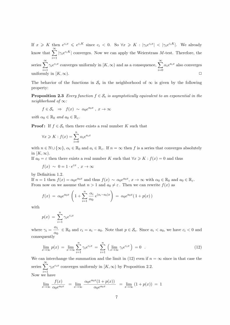
If x > K then ecix 6 eciK since ci < 0. So ∀x > K : |γiecix| < |γieciK |. We already
know that∞∑
i=1
|γieciK | converges. Now we can apply the Weierstrass M -test. Therefore, the
series∞∑
i=1
γiecix converges uniformly in [K,∞) and as a consequence,
∞∑
i=0
αieaix also converges
uniformly in [K,∞). 2
The behavior of the functions in Se in the neighborhood of ∞ is given by the followingproperty:
Proposition 2.3 Every function f ∈ Se is asymptotically equivalent to an exponential in theneighborhood of ∞:
f ∈ Se ⇒ f(x) ∼ α0ea0x , x → ∞
with α0 ∈ R0 and a0 ∈ Rε.
Proof : If f ∈ Se then there exists a real number K such that
∀x > K : f(x) =n∑
i=0
αieaix
with n ∈ N∪{∞}, αi ∈ R0 and ai ∈ Rε. If n = ∞ then f is a series that converges absolutelyin [K,∞).If a0 = ε then there exists a real number K such that ∀x > K : f(x) = 0 and thus
f(x) ∼ 0 = 1 · eεx , x → ∞
by Definition 1.2.If n = 1 then f(x) = α0e
a0x and thus f(x) ∼ α0ea0x, x → ∞ with α0 ∈ R0 and a0 ∈ Rε.
From now on we assume that n > 1 and a0 6= ε . Then we can rewrite f(x) as
f(x) = α0ea0x
(
1 +n∑
i=1
αi
α0e(ai−a0)x
)
= α0ea0x( 1 + p(x) )
with
p(x) =n∑
i=1
γiecix
where γi =αi
α0∈ R0 and ci = ai − a0. Note that p ∈ Se. Since ai < a0, we have ci < 0 and
consequently
limx→∞
p(x) = limx→∞
n∑
i=1
γiecix =
n∑
i=1
(
limx→∞
γiecix)
= 0 . (12)
We can interchange the summation and the limit in (12) even if n = ∞ since in that case the
series∞∑
i=1
γiecix converges uniformly in [K,∞) by Proposition 2.2.
Now we have
limx→∞
f(x)
α0ea0x= lim
x→∞
α0ea0x(1 + p(x))
α0ea0x= lim
x→∞(1 + p(x)) = 1
7
and thus
f(x) ∼ α0ea0x , x → ∞
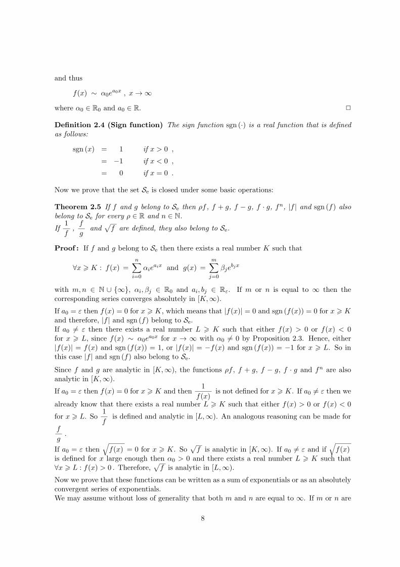
where α0 ∈ R0 and a0 ∈ R. 2
Definition 2.4 (Sign function) The sign function sgn (·) is a real function that is definedas follows:
sgn (x) = 1 if x > 0 ,
= −1 if x < 0 ,
= 0 if x = 0 .
Now we prove that the set Se is closed under some basic operations:
Theorem 2.5 If f and g belong to Se then ρf , f + g, f − g, f · g, fn, |f | and sgn (f) alsobelong to Se for every ρ ∈ R and n ∈ N.
If1
f,f
gand
√
f are defined, they also belong to Se.
Proof : If f and g belong to Se then there exists a real number K such that
∀x > K : f(x) =n∑
i=0
αieaix and g(x) =
m∑
j=0
βjebjx
with m,n ∈ N ∪ {∞}, αi, βj ∈ R0 and ai, bj ∈ Rε. If m or n is equal to ∞ then thecorresponding series converges absolutely in [K,∞).
If a0 = ε then f(x) = 0 for x > K, which means that |f(x)| = 0 and sgn (f(x)) = 0 for x > Kand therefore, |f | and sgn (f) belong to Se.If a0 6= ε then there exists a real number L > K such that either f(x) > 0 or f(x) < 0for x > L, since f(x) ∼ α0e
a0x for x → ∞ with α0 6= 0 by Proposition 2.3. Hence, either|f(x)| = f(x) and sgn (f(x)) = 1, or |f(x)| = −f(x) and sgn (f(x)) = −1 for x > L. So inthis case |f | and sgn (f) also belong to Se.
Since f and g are analytic in [K,∞), the functions ρf , f + g, f − g, f · g and fn are alsoanalytic in [K,∞).
If a0 = ε then f(x) = 0 for x > K and then1
f(x)is not defined for x > K. If a0 6= ε then we
already know that there exists a real number L > K such that either f(x) > 0 or f(x) < 0
for x > L. So1
fis defined and analytic in [L,∞). An analogous reasoning can be made for
f
g.
If a0 = ε then√
f(x) = 0 for x > K. So√
f is analytic in [K,∞). If a0 6= ε and if√
f(x)is defined for x large enough then α0 > 0 and there exists a real number L > K such that∀x > L : f(x) > 0 . Therefore,
√
f is analytic in [L,∞).
Now we prove that these functions can be written as a sum of exponentials or as an absolutelyconvergent series of exponentials.We may assume without loss of generality that both m and n are equal to ∞. If m or n are
8
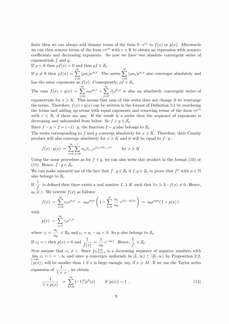
finite then we can always add dummy terms of the form 0 · eεx to f(x) or g(x). Afterwardswe can then remove terms of the form reεx with r ∈ R to obtain an expression with nonzerocoefficients and decreasing exponents. So now we have two absolute convergent series ofexponentials f and g.If ρ = 0 then ρf(x) = 0 and thus ρf ∈ Se.
If ρ 6= 0 then ρf(x) =∞∑
i=0
(ραi)eaix. The series
∞∑
i=0
(ραi)eaix also converges absolutely and
has the same exponents as f(x). Consequently, ρf ∈ Se.
The sum f(x) + g(x) =∞∑
i=0
αieaix +
∞∑
j=0
βjebjx is also an absolutely convergent series of
exponentials for x > K. This means that sum of this series does not change if we rearrangethe terms. Therefore, f(x)+g(x) can be written in the format of Definition 2.1 by reorderingthe terms and adding up terms with equal exponents and removing terms of the form reεx
with r ∈ R, if there are any. If the result is a series then the sequence of exponents isdecreasing and unbounded from below. So f + g ∈ Se.
Since f − g = f + (−1) · g, the function f − g also belongs to Se.
The series corresponding to f and g converge absolutely for x > K. Therefore, their Cauchyproduct will also converge absolutely for x > K and it will be equal to f · g :
f(x) · g(x) =∞∑
i=0
i∑
j=0
αjβi−je(aj+bi−j)x for x > K .
Using the same procedure as for f + g, we can also write this product in the format (10) or(11). Hence, f · g ∈ Se.
We can make repeated use of the fact that f · g ∈ Se if f, g ∈ Se to prove that fn with n ∈ N
also belongs to Se.
If1
fis defined then there exists a real number L > K such that ∀x > L : f(x) 6= 0. Hence,
a0 6= ε. We rewrite f(x) as follows:
f(x) =∞∑
i=0
αieaix = α0e
a0x
(
1 +∞∑
i=1
αi
α0e(ai−a0)x
)
= α0ea0x( 1 + p(x) )
with
p(x) =∞∑
i=1
γiecix
where γi =αi
α0∈ R0 and ci = ai − a0 < 0. So p also belongs to Se.
If c1 = ε then p(x) = 0 and1
f(x)=
1
α0e−a0x. Hence,
1
f∈ Se.
Now assume that c1 6= ε. Since {ci}∞i=1 is a decreasing sequence of negative numbers withlimi→∞
ci = ε = −∞ and since p converges uniformly in [L,∞) ⊂ [K,∞) by Proposition 2.2,
| p(x) | will be smaller than 1 if x is large enough, say, if x > M . If we use the Taylor series
expansion of1
1 + x, we obtain
1
1 + p(x)=
∞∑
k=0
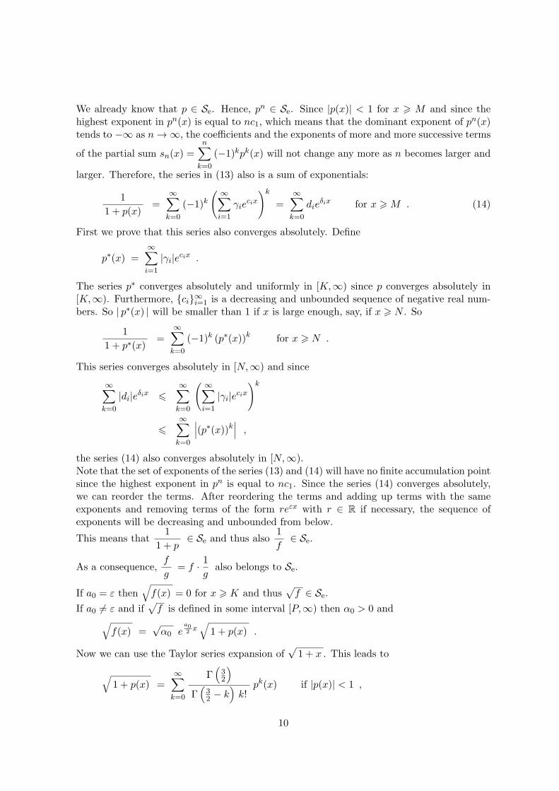
(−1)kpk(x) if |p(x)| < 1 . (13)
9
We already know that p ∈ Se. Hence, pn ∈ Se. Since |p(x)| < 1 for x > M and since thehighest exponent in pn(x) is equal to nc1, which means that the dominant exponent of pn(x)tends to −∞ as n → ∞, the coefficients and the exponents of more and more successive terms
of the partial sum sn(x) =n∑
k=0
(−1)kpk(x) will not change any more as n becomes larger and
larger. Therefore, the series in (13) also is a sum of exponentials:
1
1 + p(x)=
∞∑
k=0
(−1)k(
∞∑
i=1
γiecix
)k
=∞∑
k=0
dieδix for x > M . (14)
First we prove that this series also converges absolutely. Define
p∗(x) =∞∑
i=1
|γi|ecix .
The series p∗ converges absolutely and uniformly in [K,∞) since p converges absolutely in[K,∞). Furthermore, {ci}∞i=1 is a decreasing and unbounded sequence of negative real num-bers. So | p∗(x) | will be smaller than 1 if x is large enough, say, if x > N . So
1
1 + p∗(x)=
∞∑
k=0
(−1)k (p∗(x))k for x > N .
This series converges absolutely in [N,∞) and since
∞∑
k=0
|di|eδix 6
∞∑
k=0
(
∞∑
i=1
|γi|ecix)k
6
∞∑
k=0
∣
∣
∣(p∗(x))k∣
∣
∣ ,
the series (14) also converges absolutely in [N,∞).Note that the set of exponents of the series (13) and (14) will have no finite accumulation pointsince the highest exponent in pn is equal to nc1. Since the series (14) converges absolutely,we can reorder the terms. After reordering the terms and adding up terms with the sameexponents and removing terms of the form reεx with r ∈ R if necessary, the sequence ofexponents will be decreasing and unbounded from below.
This means that1
1 + p∈ Se and thus also
1
f∈ Se.
As a consequence,f
g= f · 1
galso belongs to Se.
If a0 = ε then√
f(x) = 0 for x > K and thus√
f ∈ Se.
If a0 6= ε and if√
f is defined in some interval [P,∞) then α0 > 0 and√
f(x) =√α0 e
a02x√
1 + p(x) .
Now we can use the Taylor series expansion of√1 + x . This leads to
√
1 + p(x) =∞∑
k=0
Γ(
32
)
Γ(
32 − k
)
k!pk(x) if |p(x)| < 1 ,
10
where Γ is the gamma function. If we apply the same reasoning as for1
1 + p, we obtain
√
1 + p ∈ Se and thus also√
f ∈ Se. 2
Now we give an alternative proof for the existence theorem of the max-algebraic SVD:
Theorem 2.6 (Existence of the singular value decomposition in Smax)Let A ∈ S
m×n and let r = min(m,n). Then there exist a max-algebraic diagonal matrixΣ ∈ R
m×nε and matrices U ∈ (S∨)m×m and V ∈ (S∨)n×n such that
A ∇ U ⊗ Σ⊗ V T (15)
with
UT ⊗ U ∇ Em
V T ⊗ V ∇ En
and ‖A‖⊕> σ1 > σ2 > . . . > σr > ε where σi = (Σ)ii.
Every decomposition of the form (15) that satisfies the above conditions is called a max-algebraic singular value decomposition of A.
Proof : If A ∈ Sm×n has entries that are not signed we can always define a signed m by n
matrix A such that
aij = aij if aij is signed,
= |aij |⊕ if aij is not signed.
Since |aij |⊕ = |aij |⊕ for all i, j, we have ‖A‖⊕= ‖A‖
⊕. Furthermore, ∀a, b ∈ S : a ∇ b ⇒
a• ∇ b, which means that A ∇ U ⊗ Σ ⊗ V T would imply A ∇ U ⊗ Σ ⊗ V T . Therefore, it issufficient to prove this theorem for signed matrices A.
So from now on we assume that A is signed. First we define c = ‖A‖⊕.
If c = ε then A = εm×n. If we take U = Em, Σ = εm×n and V = En , we have A =U ⊗ Σ ⊗ V T , UT ⊗ U = Em , V T ⊗ V = En and σ1 = σ2 = . . . = σr = ε = ‖A‖
⊕. So
U ⊗ Σ⊗ V T is a max-algebraic SVD of A.
From now on we assume that c 6= ε. We may also assume without loss of generality thatm 6 n. If m > n then we can apply the subsequent reasoning on AT since A ∇ U ⊗ Σ⊗ V T
if and only if AT ∇ V ⊗ ΣT ⊗ UT . So U ⊗ Σ⊗ V T is a max-algebraic SVD of A if and only
if V ⊗ ΣT ⊗ UT is a max-algebraic SVD of AT .
Now we have to distinguish between two different situations depending on whether or not allthe aij ’s have a finite max-absolute value.
Case 1: all the aij ’s have a finite max-absolute value.
We construct a matrix-valued function A(·) = F(A, ·). Hence, we have aij(s) = γijecijs
for all s ∈ R with γij ∈ R0 and cij = |aij |⊕ ∈ Rε.
We select the coefficients γij such that the generic rank of A(·) ism. This can be effectuatedby choosing the γij ’s such that
rank A(0) = rank Γ = m (16)
11
where (Γ)ij = γij , since the rank of A(·) is constant except in some non-generic pointswhere the rank drops. Therefore, condition (16) ensures that the generic rank of A(·) ism and that A(·) has no singular values that are identically zero.Furthermore, ifm > 1 then we select the γij ’s such that A(s) has no multiple singular valuesexcept maybe in some non-generic points. This condition will guarantee the asymptoticquadratic convergence of Kogbetliantz’s SVD algorithm. Since we are only interested inthe asymptotic behavior of the entries of A(s), we can always add an extra exponential ofthe form δije
dijs with dij < cij to aij(s) such that rank A(0) = rank (Γ +∆) = m if thisshould be necessary to obtain distinct singular values for almost all values of s.Now we define a matrix-valued function B(·) such that B(s) = e−(c+1)sA(s). So
bij(s) = γije−bijs + δije
−fijs for all s ∈ R
with bij = c+ 1− cij > 0 and fij = c+ 1− dij > bij . The entries of B(·) are in Se.
If I ⊂ R then U(s) Ψ(s) V T (s) is a (constant) SVD of B(s) for each s ∈ I if and only ifU(s) Σ(s) V T (s) with Σ(s) = e(c+1)sΨ(s) is a (constant) SVD of A(s) for each s ∈ I.
We shall apply Kogbetliantz’s SVD algorithm [4, 11] on B(·). This algorithm can beconsidered as an extension of Jacobi’s method for the calculation of the eigenvalue decom-position of a symmetric matrix. For a matrix B ∈ R
m×n (with m 6 n) a sequence ofmatrices is generated as follows:
X0 = Im , Y0 = In , S0 = B
Xk = GkXk−1 , Yk = HkYk−1 , Sk = GkSk−1HTk for k = 1, 2, 3, . . .
such that
‖Sk‖offdef=
√
√
√
√
∑
i 6=j
(Sk)2ij
decreases monotonously. So Sk tends more and more to a diagonal matrix as the iterationprocess progresses. If m = n then the orthogonal updating transformations Gk and Hk
are elementary rotations that are chosen such that (Sk)ikjk = (Sk)jkik = 0 for some pair ofindices (ik, jk). As a result we have
‖Sk‖2off = ‖Sk−1‖2off − (Sk−1)2ikjk
− (Sk−1)2jkik
.
If m < n and if m < jk 6 n then only Sikjk is zeroed and only one transformation is applied(the identity matrix is taken for Gk). We shall use the cyclic version of Kogbetliantz’s SVDalgorithm: the indices ik and jk are chosen such that the entries in the upper triangularpart of the Sk’s are selected row by row. If m = n, this yields the following sequence forthe pairs of indices (ik, jk):
If m < n then the last pair of indices of is (m,n). A complete cycle is called a sweep and
corresponds to N =(2n−m− 1)m
2iterations.
Note that
∀k ∈ N : B = XTk Sk Yk .
12
Since Gk and Hk are orthogonal matrices, we have
∀k ∈ N : ‖Sk‖F = ‖B‖F (17)
and
∀k ∈ N : XTk Xk = Im and Y T
k Yk = In .
If we define S = limk→∞
Sk, X = limk→∞
Xk and Y = limk→∞
Yk then S is a diagonal matrix and
X and Y are orthogonal matrices. After applying a permutation such that the diagonalentries of S are ordered we obtain an SVD of B:
B =(
XTP T)
·(
PSP T)
· (PY ) = UΨV T
with U = XTP T , Ψ = PSP T and V = Y TP T and where P is a permutation matrix.The convergence of the cyclic Kogbetliantz algorithm is quadratic for k large enough [15]:
∃K ∈ N such that ∀k > K : ‖Sk+N‖off 6 c ‖Sk‖2off . (18)
The operations used in Kogbetliantz’s SVD algorithm are additions, multiplications, sub-tractions, divisions, square roots, absolute values and sign functions. So if we apply thisalgorithm to a matrix with entries in Se then the entries of all the matrices generatedduring the iteration process also belong to Se by Theorem 2.5.If f , g and h belong to Se, they are asymptotically equivalent to an exponential in theneighborhood of ∞ by Proposition 2.3. So if L is large enough, then f(L) > 0 andg(L) > h(L) imply that ∀s > L : f(s) > 0 and g(s) > h(s). This is one of the reasons thatKogbetliantz’s SVD algorithm also works for matrices with entries in Se instead of in R.Now we apply Kogbetliantz’s SVD algorithm on B(·). Let Sk(·), Xk(·) and Yk(·) be thematrix-valued functions obtained in the kth step of the algorithm. Let Ψk(·), Uk(·) andVk(·) be the permuted versions of Sk(·), Xk(·) and Yk(·) respectively.The exponents of the entries of B(·) are negative and the same holds for the exponents ofthe entries of Sk(·) since ‖Sk(·)‖F = ‖B(·)‖F by (17). Hence, (18) means that the largestoff-diagonal exponent approximately doubles each N steps. Since the Frobenius norm ofSk(·) stays constant during the iteration, the exponents of the updates of the diagonalentries also approximately double each N steps. Therefore, more and more successiveterms of the series of the diagonal entries of Sk(·) stay constant as the iteration processprogresses. This also holds for the series of the entries of Xk(·) and Yk(·).In theory we should run the iteration process forever. However, since we are only interestedin the asymptotic behavior of the singular values and the entries of the singular vectors wecan stop the iteration as soon as the dominant exponents do not change anymore, i.e. aftera finite number of iteration steps.
If U(·) Ψ(·) V T (·) is a path of (approximate) SVDs of B(·) on some interval [L,∞) thatwas obtained by the above procedure, then the entries of U(·), Ψ(·) and V (·) are in Se andU(s) and V (s) are orthogonal for each s ∈ [L,∞).Furthermore, it should be pointed out that we are not really interested in a path of exactSVDs of B(·). Let ∆k(·) be the diagonal matrix-valued function obtained by removing the
13
off-diagonal entries from Ψk(·) after the kth iteration step. If we define the matrix-valuedfunction Ck(·) = Uk(·) ∆k(·) V T
k (·), then we have a path of exact SVDs of C(·) on someinterval [L,∞). This means that we could also stop the iteration process as soon as
bij(s) ∼ cij(s) , s → ∞ for all i, j .
Define a matrix-valued function Σ(·) such that Σ(s) = e(c+1)sΨ(s). Then U(·) Σ(·) V T (·)is a path of (approximate) SVDs of A(·) on [L,∞):
A(s) ∼ U(s) Σ(s) V T (s) , s → ∞ (19)
UT (s) U(s) = Im if s > L (20)
V T (s) V (s) = In if s > L . (21)
So now we have proved that there exists a path of (approximate) SVDs of A(·) for which thesingular values and the entries of the singular vectors belong to Se and are asymptoticallyequivalent to an exponential in the neighborhood of ∞ by Proposition 2.3.If we apply the reverse mapping R, we obtain a max-algebraic SVD of A. Since we haveused numbers instead of parameters for the coefficients of the exponentials in F(A, ·), thecoefficients of the exponentials in the singular values and the entries of the singular vectorsare also numbers. Therefore, the reverse mapping only yields signed results. If we define
Σ = R(
Σ(·))
, U = R(
U(·))
, V = R(
V (·))
and σi = (Σ)ii = R(σi(·)) ,
then Σ is a max-algebraic diagonal matrix and U and V have signed entries. If we applythe reverse mapping R to (19) – (21), we get
A ∇ U ⊗ Σ⊗ V T
UT ⊗ U ∇ Em
V T ⊗ V ∇ En .
The σi(·)’s are positive in [L,∞) and therefore, σi ∈ Rε. Since the σi(·)’s are ordered in[L,∞), their dominant exponentials are also ordered. Hence, σ1 > σ2 > . . . > σr > ε.We have ‖A(s)‖F ∼ γecs, s → ∞ with γ > 0 since c = ‖A‖
⊕is the largest exponent that
appears in the entries of A(·). So R(
‖A(·)‖F)
= c = ‖A‖⊕. If M ∈ R
m×n then
1√n
‖M‖F 6 ‖M‖2 6 ‖M‖F .
Hence,
1√n‖A(s)‖F 6 ‖A(s)‖2 6 ‖A(s)‖F if s > L .
Since σ1(s) ∼ ‖A(s)‖2, s → ∞ and since the mapping R preserves the order, this leadsto ‖A‖
⊕6 σ1 6 ‖A‖
⊕and consequently, σ1 = ‖A‖
⊕.
14
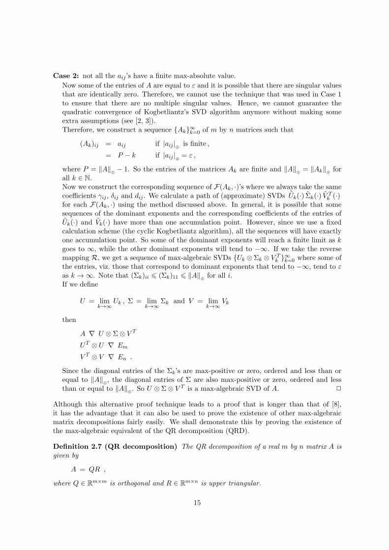
Case 2: not all the aij ’s have a finite max-absolute value.
Now some of the entries of A are equal to ε and it is possible that there are singular valuesthat are identically zero. Therefore, we cannot use the technique that was used in Case 1to ensure that there are no multiple singular values. Hence, we cannot guarantee thequadratic convergence of Kogbetliantz’s SVD algorithm anymore without making someextra assumptions (see [2, 3]).Therefore, we construct a sequence {Ak}∞k=0 of m by n matrices such that
(Ak)ij = aij if |aij |⊕ is finite ,
= P − k if |aij |⊕ = ε ,
where P = ‖A‖⊕− 1. So the entries of the matrices Ak are finite and ‖A‖
⊕= ‖Ak‖⊕
forall k ∈ N.Now we construct the corresponding sequence of F(Ak, ·)’s where we always take the samecoefficients γij , δij and dij . We calculate a path of (approximate) SVDs Uk(·) Σk(·) V T
k (·)for each F(Ak, ·) using the method discussed above. In general, it is possible that somesequences of the dominant exponents and the corresponding coefficients of the entries ofUk(·) and Vk(·) have more than one accumulation point. However, since we use a fixedcalculation scheme (the cyclic Kogbetliantz algorithm), all the sequences will have exactlyone accumulation point. So some of the dominant exponents will reach a finite limit as kgoes to ∞, while the other dominant exponents will tend to −∞. If we take the reversemapping R, we get a sequence of max-algebraic SVDs {Uk ⊗Σk ⊗ V T
k }∞k=0 where some ofthe entries, viz. those that correspond to dominant exponents that tend to −∞, tend to εas k → ∞. Note that (Σk)ii 6 (Σk)11 6 ‖A‖
⊕for all i.
If we define
U = limk→∞
Uk , Σ = limk→∞
Σk and V = limk→∞
Vk
then
A ∇ U ⊗ Σ⊗ V T
UT ⊗ U ∇ Em
V T ⊗ V ∇ En .
Since the diagonal entries of the Σk’s are max-positive or zero, ordered and less than orequal to ‖A‖
⊕, the diagonal entries of Σ are also max-positive or zero, ordered and less
than or equal to ‖A‖⊕. So U ⊗ Σ⊗ V T is a max-algebraic SVD of A. 2
Although this alternative proof technique leads to a proof that is longer than that of [8],it has the advantage that it can also be used to prove the existence of other max-algebraicmatrix decompositions fairly easily. We shall demonstrate this by proving the existence ofthe max-algebraic equivalent of the QR decomposition (QRD).
Definition 2.7 (QR decomposition) The QR decomposition of a real m by n matrix A isgiven by
A = QR ,
where Q ∈ Rm×m is orthogonal and R ∈ R
m×n is upper triangular.
15
Note that ‖A‖F = ‖R‖F since Q is an orthogonal matrix.
Theorem 2.8 If A(·) ∈ (Se)m×n then there exists a path of QR factorizations Q(·) R(·) of
A(·) for which the entries of Q(·) and R(·) also belong to Se.
Proof : We can use Householder or Givens transformations to calculate the QR decomposi-tion of a matrix [10]. If we apply the algorithms in their most elementary form (i.e. withoutthe refinements necessary to avoid overflow and to guarantee numerical stability), we onlyhave to use additions, multiplications, subtractions, divisions and square roots. Hence, theentries of resulting matrices Q(·) and R(·) belong to Se by Theorem 2.5. 2
As a direct consequence we have
Theorem 2.9 (Max-algebraic QR decomposition) If A ∈ Sm×n then there exist a ma-
trix Q ∈ (S∨)m×m and a max-algebraic upper triangular matrix R ∈ (S∨)m×n such that
A ∇ Q⊗R (22)
with
QT ⊗Q ∇ Em
and ‖R‖⊕6 ‖A‖
⊕.
Every decomposition of the form (22) that satisfies the above conditions is called a max-algebraic QR decomposition of A.
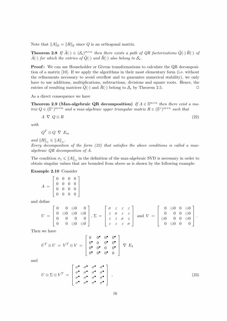
The condition σ1 6 ‖A‖⊕in the definition of the max-algebraic SVD is necessary in order to
obtain singular values that are bounded from above as is shown by the following example:
Example 2.10 Consider
A =
0 0 0 00 0 0 00 0 0 00 0 0 0
and define
U =
0 0 ⊖0 00 ⊖0 ⊖0 ⊖00 0 0 00 0 ⊖0 ⊖0
, Σ =
σ ε ε εε σ ε εε ε σ εε ε ε σ
and V =
0 ⊖0 0 ⊖00 0 0 ⊖0
⊖0 0 0 ⊖00 ⊖0 0 0
.
Then we have
UT ⊗ U = V T ⊗ V =
0 0• 0• 0•
0• 0 0• 0•
0• 0• 0 0•
0• 0• 0• 0
∇ E4
and
U ⊗ Σ⊗ V T =
σ• σ• σ• σ•
σ• σ• σ• σ•
σ• σ• σ• σ•
σ• σ• σ• σ•
, (23)
16
which means that U ⊗ Σ⊗ V T ∇ A for every σ > 0.So if the condition σ1 6 ‖A‖
⊕would not be included in the definition of the max-algebraic
SVD, (23) would be a max-algebraic SVD of A for every σ > 0. 2
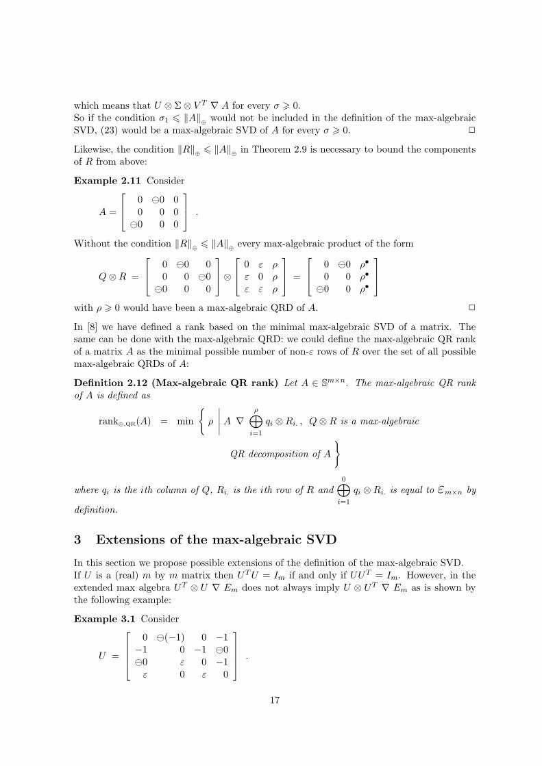
Likewise, the condition ‖R‖⊕6 ‖A‖
⊕in Theorem 2.9 is necessary to bound the components
of R from above:
Example 2.11 Consider
A =
0 ⊖0 00 0 0
⊖0 0 0
.
Without the condition ‖R‖⊕6 ‖A‖
⊕every max-algebraic product of the form
Q⊗R =
0 ⊖0 00 0 ⊖0
⊖0 0 0
⊗
0 ε ρε 0 ρε ε ρ
=
0 ⊖0 ρ•
0 0 ρ•
⊖0 0 ρ•
with ρ > 0 would have been a max-algebraic QRD of A. 2
In [8] we have defined a rank based on the minimal max-algebraic SVD of a matrix. Thesame can be done with the max-algebraic QRD: we could define the max-algebraic QR rankof a matrix A as the minimal possible number of non-ε rows of R over the set of all possiblemax-algebraic QRDs of A:
Definition 2.12 (Max-algebraic QR rank) Let A ∈ Sm×n. The max-algebraic QR rank
of A is defined as
rank⊕,QR(A) = min
{
ρ
∣
∣
∣
∣
∣
A ∇ρ⊕
i=1
qi ⊗Ri. , Q⊗R is a max-algebraic
QR decomposition of A
}
where qi is the ith column of Q, Ri. is the ith row of R and0⊕
i=1
qi ⊗Ri. is equal to εm×n by
definition.
3 Extensions of the max-algebraic SVD
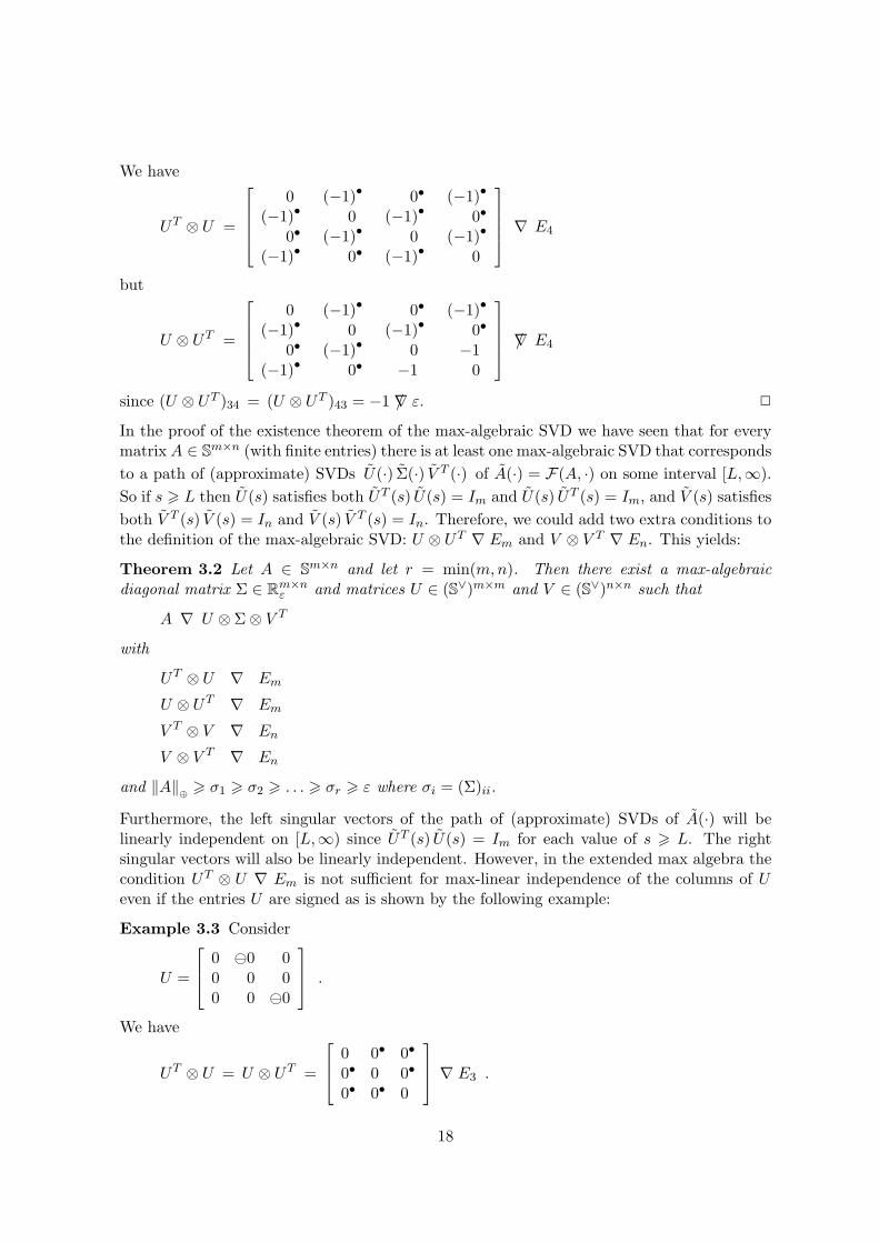
In this section we propose possible extensions of the definition of the max-algebraic SVD.If U is a (real) m by m matrix then UTU = Im if and only if UUT = Im. However, in theextended max algebra UT ⊗ U ∇ Em does not always imply U ⊗ UT ∇ Em as is shown bythe following example:
Example 3.1 Consider
U =
0 ⊖(−1) 0 −1−1 0 −1 ⊖0⊖0 ε 0 −1ε 0 ε 0
.
17
We have
UT ⊗ U =
0 (−1)• 0• (−1)•
(−1)• 0 (−1)• 0•
0• (−1)• 0 (−1)•
(−1)• 0• (−1)• 0
∇ E4
but
U ⊗ UT =
0 (−1)• 0• (−1)•
(−1)• 0 (−1)• 0•
0• (−1)• 0 −1(−1)• 0• −1 0
∇/ E4
since (U ⊗ UT )34 = (U ⊗ UT )43 = −1 ∇/ ε. 2
In the proof of the existence theorem of the max-algebraic SVD we have seen that for everymatrix A ∈ S
m×n (with finite entries) there is at least one max-algebraic SVD that corresponds
to a path of (approximate) SVDs U(·) Σ(·) V T (·) of A(·) = F(A, ·) on some interval [L,∞).
So if s > L then U(s) satisfies both UT (s) U(s) = Im and U(s) UT (s) = Im, and V (s) satisfies
both V T (s) V (s) = In and V (s) V T (s) = In. Therefore, we could add two extra conditions tothe definition of the max-algebraic SVD: U ⊗ UT ∇ Em and V ⊗ V T ∇ En. This yields:
Theorem 3.2 Let A ∈ Sm×n and let r = min(m,n). Then there exist a max-algebraic
diagonal matrix Σ ∈ Rm×nε and matrices U ∈ (S∨)m×m and V ∈ (S∨)n×n such that
A ∇ U ⊗ Σ⊗ V T
with
UT ⊗ U ∇ Em
U ⊗ UT ∇ Em
V T ⊗ V ∇ En
V ⊗ V T ∇ En
and ‖A‖⊕> σ1 > σ2 > . . . > σr > ε where σi = (Σ)ii.
Furthermore, the left singular vectors of the path of (approximate) SVDs of A(·) will belinearly independent on [L,∞) since UT (s) U(s) = Im for each value of s > L. The rightsingular vectors will also be linearly independent. However, in the extended max algebra thecondition UT ⊗ U ∇ Em is not sufficient for max-linear independence of the columns of Ueven if the entries U are signed as is shown by the following example:
Example 3.3 Consider
U =
0 ⊖0 00 0 00 0 ⊖0
.
We have
UT ⊗ U = U ⊗ UT =
0 0• 0•
0• 0 0•
0• 0• 0
∇ E3 .
18
Furthermore, det⊕ U = 0•. So by Theorem 1.10 there exists a signed solution of α1 ⊗ u1 ⊕α2 ⊗ u2 ⊕ α3 ⊗ u3 ∇ ε3×1, viz. α1 = 0, α2 = ⊖0 and α3 = ⊖0. Therefore, the vectors u1, u2and u3 are max-linearly dependent by Definition 1.11. 2
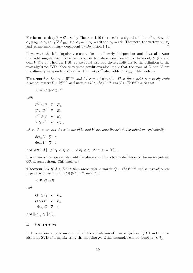
If we want the left singular vectors to be max-linearly independent and if we also wantthe right singular vectors to be max-linearly independent, we should have det⊕ U ∇/ ε anddet⊕ V ∇/ ε by Theorem 1.10. So we could also add these conditions to the definition of themax-algebraic SVD. Note that these conditions also imply that the rows of U and V aremax-linearly independent since det⊕ U = det⊕ UT also holds in Smax. This leads to:
Theorem 3.4 Let A ∈ Sm×n and let r = min(m,n). Then there exist a max-algebraic
diagonal matrix Σ ∈ Rm×nε and matrices U ∈ (S∨)m×m and V ∈ (S∨)n×n such that
A ∇ U ⊗ Σ⊗ V T
with
UT ⊗ U ∇ Em
U ⊗ UT ∇ Em
V T ⊗ V ∇ En
V ⊗ V T ∇ En ,
where the rows and the columns of U and V are max-linearly independent or equivalently
det⊕ U ∇/ ε
det⊕ V ∇/ ε
and with ‖A‖⊕> σ1 > σ2 > . . . > σr > ε, where σi = (Σ)ii.
It is obvious that we can also add the above conditions to the definition of the max-algebraicQR decomposition. This leads to:
Theorem 3.5 If A ∈ Sm×n then there exist a matrix Q ∈ (S∨)m×m and a max-algebraic
upper triangular matrix R ∈ (S∨)m×n such that
A ∇ Q⊗R
with
QT ⊗Q ∇ Em
Q⊗QT ∇ Em
det⊕ Q ∇/ ε
and ‖R‖⊕6 ‖A‖
⊕.
4 Examples
In this section we give an example of the calculation of a max-algebraic QRD and a max-algebraic SVD of a matrix using the mapping F . Other examples can be found in [8, 7].
19
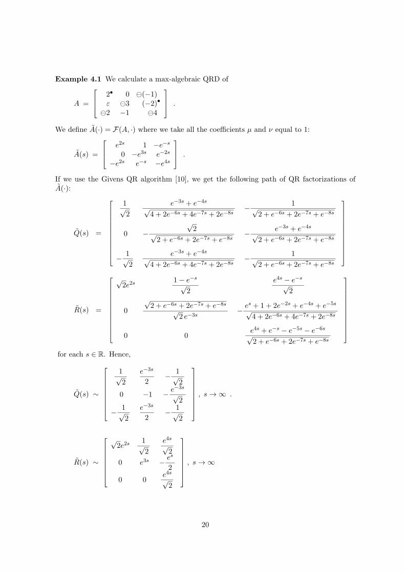
Example 4.1 We calculate a max-algebraic QRD of
A =
2• 0 ⊖(−1)ε ⊖3 (−2)•
⊖2 −1 ⊖4
.
We define A(·) = F(A, ·) where we take all the coefficients µ and ν equal to 1:
A(s) =
e2s 1 −e−s
0 −e3s e−2s
−e2s e−s −e4s
.
If we use the Givens QR algorithm [10], we get the following path of QR factorizations ofA(·):
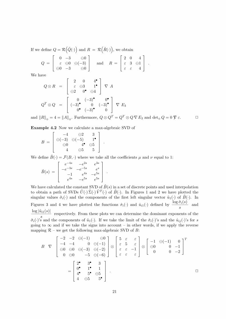
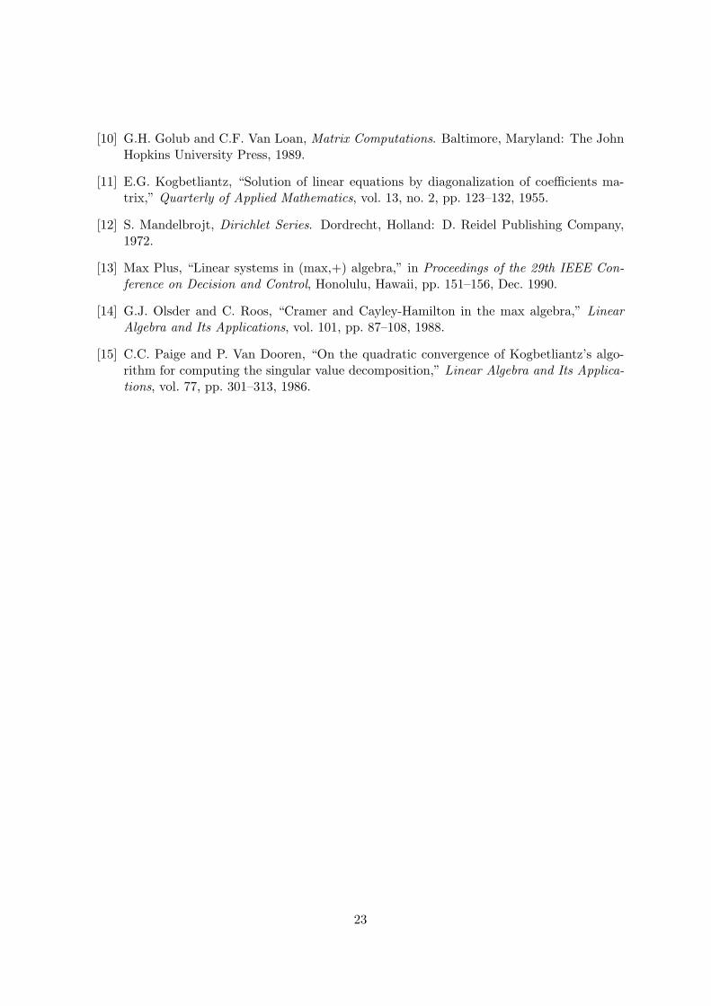
Example 4.2 Now we calculate a max-algebraic SVD of
B =
−4 ⊖2 3⊖(−3) ⊖(−5) 1•
⊖0 4• ⊖54 ⊖5 5
.
We define B(·) = F(B, ·) where we take all the coefficients µ and ν equal to 1:
B(s) =
e−4s −e2s e3s
−e−3s −e−5s es
−1 e4s −e5s
e4s −e5s e5s
.
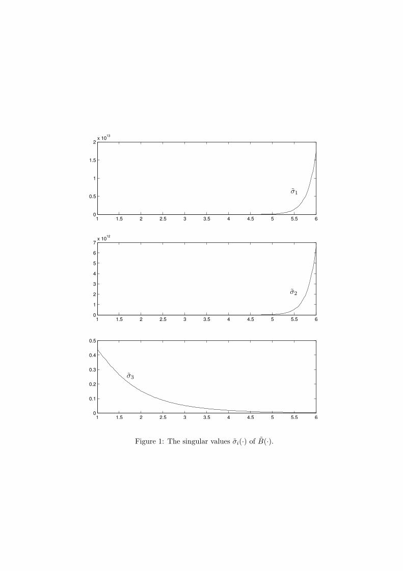
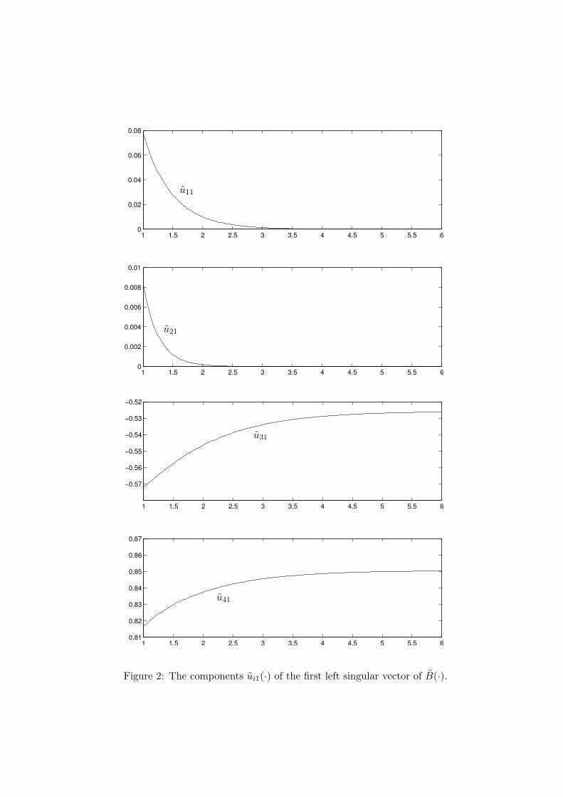
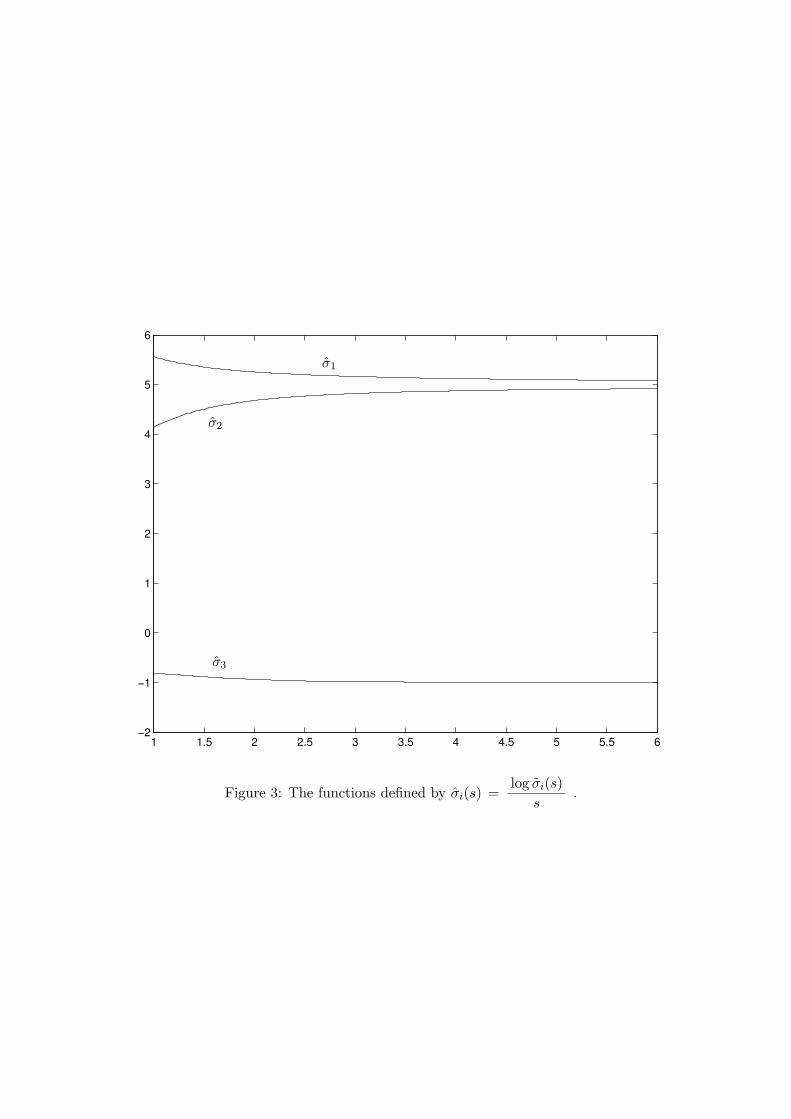
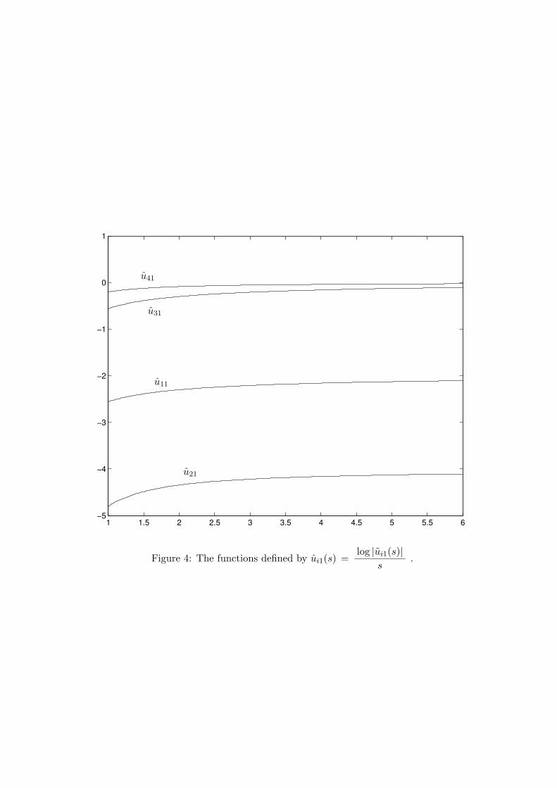
We have calculated the constant SVD of B(s) in a set of discrete points and used interpolationto obtain a path of SVDs U(·) Σ(·) V T (·) of B(·). In Figures 1 and 2 we have plotted thesingular values σi(·) and the components of the first left singular vector u1(·) of B(·). In
Figures 3 and 4 we have plotted the functions σi(·) and ui1(·) defined bylog σi(s)
sand
log |ui1(s)|s
respectively. From these plots we can determine the dominant exponents of the
σi(·)’s and the components of u1(·). If we take the limit of the σi(·)’s and the uij(·)’s for sgoing to ∞ and if we take the signs into account – in other words, if we apply the reversemapping R – we get the following max-algebraic SVD of B:
B ∇
−2 −2 ⊖(−1) ⊖0
−4 −4 0 ⊖(−1)
⊖0 ⊖0 ⊖(−3) ⊖(−2)
0 ⊖0 −5 ⊖(−6)
⊗
5 ε εε 5 εε ε −1ε ε ε
⊗
−1 ⊖(−1) 0⊖0 0 −10 0 −2
T
=
2• 3• 30• 1• 14• 5• ⊖54 ⊖5 5•
. 2
21
5 Conclusions and future research
First we have proved the existence of a kind of singular value decomposition (SVD) in theextended max algebra. Next we have used the same proof technique to prove the existenceof a QR factorization of a matrix in the extended max algebra. It is obvious that this prooftechnique can also be used to prove the existence of max-algebraic equivalents of many othermatrix decompositions from linear algebra: it can easily be adapted to prove the existence ofan LU decomposition of a matrix in the extended max algebra and to prove the existence of aneigenvalue decomposition for symmetric matrices in the extended max algebra (by using theJacobi algorithm for the calculation of the eigenvalue decomposition of a symmetric matrix).We have also discussed some possible extensions of the definition of the max-algebraic SVD.
Topics for future research are: further investigation of the properties of the max-algebraicSVD and the max-algebraic QR decomposition, extension of the proof technique of this paperto prove the existence of other max-algebraic matrix decompositions and investigation ofpossible applications of these matrix decompositions.
References
[1] F. Baccelli, G. Cohen, G.J. Olsder, and J.P. Quadrat, Synchronization and Linearity.New York: John Wiley & Sons, 1992.
[2] Z. Bai, “Note on the quadratic convergence of Kogbetliantz’s algorithm for computingthe singular value decomposition,” Linear Algebra and Its Applications, vol. 104, pp. 131–140, 1988.
[3] J.P. Charlier and P. Van Dooren, “On Kogbetliantz’s SVD algorithm in the presence ofclusters,” Linear Algebra and Its Applications, vol. 95, pp. 135–160, 1987.
[4] J.P. Charlier, M. Vanbegin, and P. Van Dooren, “On efficient implementations of Kog-betliantz’s algorithm for computing the singular value decomposition,” NumerischeMathematik, vol. 52, pp. 279–300, 1988.
[5] G. Cohen, D. Dubois, J.P. Quadrat, and M. Viot, “A linear-system-theoretic view ofdiscrete-event processes and its use for performance evaluation in manufacturing,” IEEETransactions on Automatic Control, vol. 30, no. 3, pp. 210–220, Mar. 1985.
[6] R.A. Cuninghame-Green, Minimax Algebra, vol. 166 of Lecture Notes in Economics andMathematical Systems. Berlin, Germany: Springer-Verlag, 1979.
[7] B. De Schutter and B. De Moor, “The singular value decomposition in the extended maxalgebra is an extended linear complementarity problem,” Tech. rep. 95-07, ESAT-SISTA,K.U.Leuven, Leuven, Belgium, Mar. 1995.
[8] B. De Schutter and B. De Moor, “The singular value decomposition in the extended maxalgebra,” Linear Algebra and Its Applications, vol. 250, pp. 143–176, Jan. 1997.
[9] S. Gaubert, Theorie des Systemes Lineaires dans les Dioıdes. PhD thesis, Ecole NationaleSuperieure des Mines de Paris, France, July 1992.
22
[10] G.H. Golub and C.F. Van Loan, Matrix Computations. Baltimore, Maryland: The JohnHopkins University Press, 1989.
[11] E.G. Kogbetliantz, “Solution of linear equations by diagonalization of coefficients ma-trix,” Quarterly of Applied Mathematics, vol. 13, no. 2, pp. 123–132, 1955.
[12] S. Mandelbrojt, Dirichlet Series. Dordrecht, Holland: D. Reidel Publishing Company,1972.
[13] Max Plus, “Linear systems in (max,+) algebra,” in Proceedings of the 29th IEEE Con-ference on Decision and Control, Honolulu, Hawaii, pp. 151–156, Dec. 1990.
[14] G.J. Olsder and C. Roos, “Cramer and Cayley-Hamilton in the max algebra,” LinearAlgebra and Its Applications, vol. 101, pp. 87–108, 1988.
[15] C.C. Paige and P. Van Dooren, “On the quadratic convergence of Kogbetliantz’s algo-rithm for computing the singular value decomposition,” Linear Algebra and Its Applica-tions, vol. 77, pp. 301–313, 1986.
23
1 1.5 2 2.5 3 3.5 4 4.5 5 5.5 60
0.5
1
1.5
2x 10
13
1 1.5 2 2.5 3 3.5 4 4.5 5 5.5 60
1
2
3
4
5
6
7x 10
12
σ1
σ2
1 1.5 2 2.5 3 3.5 4 4.5 5 5.5 60
0.1
0.2
0.3
0.4
0.5
σ3
Figure 1: The singular values σi(·) of B(·).
1 1.5 2 2.5 3 3.5 4 4.5 5 5.5 60
0.02
0.04
0.06
0.08
1 1.5 2 2.5 3 3.5 4 4.5 5 5.5 60
0.002
0.004
0.006
0.008
0.01
u11
u21
1 1.5 2 2.5 3 3.5 4 4.5 5 5.5 6
−0.57
−0.56
−0.55
−0.54
−0.53
−0.52
1 1.5 2 2.5 3 3.5 4 4.5 5 5.5 60.81
0.82
0.83
0.84
0.85
0.86
0.87
u31
u41
Figure 2: The components ui1(·) of the first left singular vector of B(·).
1 1.5 2 2.5 3 3.5 4 4.5 5 5.5 6−2
−1
0
1
2
3
4
5
6
σ1
σ2
σ3
Figure 3: The functions defined by σi(s) =log σi(s)
s.
1 1.5 2 2.5 3 3.5 4 4.5 5 5.5 6−5
−4
−3
−2
−1
0
1
u11
u21
u31
u41
Figure 4: The functions defined by ui1(s) =log |ui1(s)|