University of Cape Town The Siting of a Wind Turbine using the WA SP Numerical Model and its Validation by Comparison with Field Data JonathanA.N. Denison April 1990 Submitted to the University of Cape Town in partial fulfilment for the degree of Master of Science in Engineering. "'-}i..·--:r-.- .-'"""-:-"'.:"\..:..,..,:-,, The nf C ·r ·,,. "r'\ '1 <'!ven : the to r ::r-., '·: • · · · ' 1 in , · tr,-.. or in part Co:·/··'. ".t · ._y t:, · ·.·)r. ·. ...... . . :. . ' t iti I SUtUn11i:ted to I iiI The the • I
Transcript
Univers
ity of
Cap
e Tow
n
The Siting of a Wind Turbine using the WA SP Numerical Model and its Validation by Comparison with Field Data
JonathanA.N. Denison
April 1990
Submitted to the University of Cape Town in partial fulfilment for the degree of Master of Science in Engineering.
The Univer~:tv nf C ·~,~ ·r ·,,. "r'\ '1 ~t;: bc~n <'!ven : the rir~ht to r ::r-., '·: • · · · ~ ' 1 ·~ -~.; in , · tr,-..
or in part Co:·/··'. ".t · ._y t:, · ·.·)r. ·. ¥~'ftl'J..i1r.-'... ...... ~ . . :. . ' ~ t
iti
I
SUtUn11i:ted to
I iiI
The the
• I
The copyright of this thesis vests in the author. No quotation from it or information derived from it is to be published without full acknowledgement of the source. The thesis is to be used for private study or non-commercial research purposes only.
Published by the University of Cape Town (UCT) in terms of the non-exclusive license granted to UCT by the author.
Univers
ity of
Cap
e Tow
n
Univers
ity of
Cap
e Tow
n
I, Jonathan Anthony Noel Denison, submit this thesis in partial fulfilment of the requirements for the degree of Master of Science in Engineering. I claim that this is my original work and that it has not been submitted in this or in a similar fonn for a degree at any other University.
Univers
ity of
Cap
e Tow
n
Acknowledgements
I would like to acknowledge the assistance and guidance provided by Professor R.K. Dutkiewicz as well as the staff at the Energy Research Institute, University of Cape Town.
The assistance and training in the use ofSACIANT provided by Anne Tregidga of the- Land Swveying Department, UCT is much appreciated. Thanks also to Lize Basson for help with the organisation of information and the final layout
Finally, I would like to thank the N.E.C. for the financial support given thus making the project possible.
6.2 Location of a WECS Site WASP ......... ' .................... 40 6.2.1 of Results ................................... 40 6.2.2 Results ...................................,...42
Turbulence of the Wind Over the :SOl~taIllysber'2 ............. ' ........... 44
Power law exponent (a) variation with season change . . . . . . . . . . . . . . . . . . . . . . . 16 . Power law exponent (a) variation with season change and time of day . . . . . . . . . . 17
The cost of wind generated electricity at nine sites (1983 values, SA c/kWhr) . . . . . . . 18
The cost of electricity in Cape Town from wind, diesel generation and the national grid . . . . .
Average annual velocity and power at the best site . . . . . . . . . . . . . . . . . . . . . . . . . 42
Vlll
1.1 vs. terrain
1.2 (zo) vs. terrain
2.1 annual """ri~nP>,·ri at four coastal
2.2 Power law with season
2.3 Power law variation with season
2.4
2.5 cost
2.6
6.1
6.2
Town
of wind enhancement on the cost of
power at the site
............... 6
............... 7
....................... 11
and time of
.............. 16
Town
17
18
18
.... 18
.... 40
..... 42
Univers
ity of
Cap
e Tow
n
Synopsis
Synopsis
A number of research projects undertaken over the last 10 years have found that Southern Africa has a signficant wind energy resource, which could be exploited to provide wind-generated electricity. An economic analysis was carried out in 1983 and it was found that wind energy was uneconomical at the time, but the results suggest that at locations with higher wind speeds, the cost of wind power would approach the South African grid electricity cost.
The objectives of this study were twofold
The first was to locate sites where the wiiid is enhanced due to orographic forcing, thus having high annual average windspeeds. The WASP numerical model was used to simulate wind speeds over the Soetanysberg, a coastal hill approximately 20 km west of Cape Agulhas. The average annual wind speed was predicted to be 11.4 m/s at 50m a.g.l at this site. This is a 24% increase over the wind measured at the Cape Agulhas lighthouse for the same height The predicted theoretical power of 2019 W/m2
, was more than twice the average power that occurs at the lighthouse.
The second aim was to validate the numerical model. This was achieved by measuring wind speeds, using a TAIA Kite, at a number of prospective sites on the Soetanysberg and at Cape Agulhas. The wind speed values from Cape Agulhas were then useg by the numerical model to make velocity predictions at the sites and these results were compared with the measured values. It was found that the numerical model performed well. 1\vo indicators were used to compare the results; the error of predictions (m) and the correlation coefficient (r). The average error of the predictions was 7%, with a maximum error of 15.4o/o, and it was found that the,model tended to underestimate the wind speed when it erred The measured velocity profile, was correlated with the predicted velocity profile and 'r' was found to range between 0.68 and 0.87 for eight of the nine sites.
It was concluded that the Soetanysberg is an area of high wind energy potential and would be a suitable site for a wind energy conversion system. In addition, the WASP numerical model can be con5idered an accurate method for assessing the wind potential in hilly terrain.
I
lX
was correlated with hPt1""PP'''' 0.68 and 0.87
It was cODlcluded
COllSi(lert:~d an accurate "'",vU"""U terrain.
I
Univers
ity of
Cap
e Tow
n Chapter 1 Introduction to Wind Energy Utilisation
Introduction to Uind Energy Utilisation 1
..
Univers
ity of
Cap
e Tow
n
1.1 Wind Energy in Historical Perspective
Wind has been utilised since ancient times to assist humankind in the menial tasks of life. Its role in water transport and grain processing dates back to the earliest civilisations. The first people to convert the wind into rotational motion were monks from ancient Tibet, " ... who invented the bladed propellor to write down the sacred messages delivered by the wind" ( 1)
-----··-------. --··
Figure 1.1: Dutch Ulindmill
The invention of the multi-bladed American farm windmill (Figure 1.2) in 1850 by Daniel Halliday made life possible in many of the drier parts of the United States. They are still the only factor that stand between farmers and ruin in many areas of Mexica, Brazil, Argentina, Australia and South Africa (2)
Wmdmills (Figure 1.1) were introduced to the Western world around the 12th centwy AD. They played a significant part in the development of Europe, pumping water in Holland and milling elsewhere, up until the birth of steam power in the 1800s.
Figure 1.2 : Multi-bladedAmerican Farm J#ndmill
The generation of electricity from the wind was first demonstrated in America in 1860 (3), but it could not compete with steam-powered electricity and the idea was only taken up on a small scale for remote lqcation power supply.
1.1.1 Wind Energy in the 20th Century
Denmark is one of the world leaders in wind energy utilisation, primarily because there are no coal deposits and limited hydro power resources. By 1890 there were 7000 windmills in operation across the country supplying a quarter of the nation's direct power needs.
At the turn of the century the Danish government embarked on a programme to develop large scale wind-powered electric generators. Power from these Wind Energy Conversion Systems (WE.CS) continued to be fed into the national grid until the last one was closed down in 1968 because the cost of electricity supplied by local wind was twice that of hydro-electric energy imported from Sweden(2) Only experimental turbines up to 200 kW in size remained in operation.
The largest windmill to be built prior to the late 1970s was located on top of Grandpa's Knob in Vermont in the United States of America. It was mounted on a 37m tower and had rotor blades
Introduction to Wind &tergy Utilisation 2
1.1
in water f"r<I,nc1".,...rt
convert the wind ..,." • ..,... ... v. to
1.1: Dutch Windmill
1.2 : Multi-bladedAmerican Farm Windmill
demonstrated in America in 1860 it <:tP·"m .• nnUlprprl "'."' ......... ,,"y and was taken up on a small
1.1.1
to late 19705 was on Vermont in the mClUnroo on a 37m tower and had rotor
Univers
ity of
Cap
e Tow
n
measuring 58m from tip to tip. It generated 1.25 Megawatts (MW) of electrical power in winds of 13 m/s and higher and ran intermittently from 1941to1945 until a blade failure caused it to shut down. The limiting factor was not a lack of technical development, but the disturbed economics due to the Second World War did not permit the system to compete with cheap oil and coal (4)
In the United Kingdom, extensive studies of wind speed and energy potential were made in the mid 50s and 100 kW prototypes were established. The results of these studies showed that winds which were consistently available on the western seaboard and the surrounding islands were capable of supplying substantial amounts of wind-generated electricity.
Major problems with equipment failure were experienced because of cyclical loading and problems associated with turbulence. This forced designers to realise that harnessing the power of the wind was more complicated than had first been believed
In the mid 1960s the French successfully developed two horizontal axis machines in the 1000 kW range. At the same time experimentation on vertical axis conversion systems, most notably the Darrius Rotor, were carried out and several were built and tested(4) Around this time several improvements in the design of wind generators were made in Germany, such as the variable pitch propellor and the use of lightweight composite blades.
Despite the growing international interest and technological developments, wind was generally not considered a major source of electrical power. The traditional sources of electrical power -coal, oil, nuclear and hydro- were well understood, cheap and reliable, which dissuaded decisionmakers from seriously examining other power sources.
1.1.2 The Oil Crisis
In 1973, the oil-producing and exporting countries imposed a global oil embargo which had major repercussions on the world's energy policies. The high price of crude which followed once the embargo was lifted, and the need for strategic self-sufficiency, forced Western governments to focus their interest on alternative energy sources.
In order to stimulate growth and investment in the wind energy industry, some governments took legislative action. The USA, for example, passed new laws whereby the public electricity supply utilities were obliged to buy power from anyone who wanted to sell it Tax concessions were granted to those investing in wind energy development. Those measures precipitated the surge in wind farm growth in the early 1980s.
Additionally, the USA government tendered contracts for the design, construction and testing of turbines of various sizes. These measures stimulated not only the American wind energy industry, but also the Danish, Dutch, Belgian, German and Swiss, as many contracts were taken up by them. At the end of 1986, many of the tax concessions had been withdrawn and investment in wind energy slowed. It seems however, that the industry in the United States has reached a level of maturity capable of surviving with less government support(5)
The rate of growth of Wmd Energy Conversion Systems (WE.CS) usage in Denmark was boosted by large discounts offered on new sales. By 1979 wind turbines provided about 2 Megawatts and, by 1986, the figure was approaching 90 Megawatts.
It is interesting to note that the USA still produces most of the world's wind-generated electricity. The total installed capacity worldwide is about 1500 Megawatts, 90% of which is generated in California.
Introduction to Uind Energy Utilisation 3
loacilng and
1
new anyone who wanted to
Qe1{eHJpInelli. Those measures "",","';r"t,.h·rl
"' .. .uu .... '''' ..... 'y not wind energy UI1LIUI>IU.Y,
as many coDlracts were taken them. tax concessions had been withdrawn and investment in wind that the in the States has a level
It is to note that the total installed \.4 .. 10. ...... ,
Univers
ity of
Cap
e Tow
n
1.1.3 International Co-operation
In order to benefit from international co-operation surrounding the problems of energy supply, the International Fn.ergy Agency (IEA) was formed in 1974. It presently comprises 21 industrial countries - 16 European countri~, as well as Australia, Canada, Japan, New Zealand and the United States. Its objectives are to find ways of reducing dependence on oil and secunng the supply of energy. This is done primarily by cooperation and task-sharing of commonly funded research projects, and by exchanging information on national activities.(6)
In the field of wind energy, the IPA co-ordinate, among other projects, a large scale WE.CS programme. It is an arrangement for information exchange and co-ordination of national activities of WE.CS, 1 MW or larger. The agreement was originally signed by the USA, Sweden, Denmark, the Federal Republic of Germany and Canada The UK and the Netherlands have since joined
IPA research is ongoing and covers the whole field of interest concerned with wind power usage. As far as the future is concerned, the potential of offshore WE.CS is under investigation as the most favourable winds are often found at sea, where the surface friction is lower than on land The wind potential of the North Sea is especially interesting to the European countries. Denmark, the Netherlands, Sweden and the UK are jointly involved in studies there.
In the distant future, some scientists have ideas to haniess the ever constant jet-streams which blow endlessly around the globe at altitudes of 10to15 kilometres. There are four main jet streams which occur where hot and cold a4 masses meet. They are wide and relatively shallow and move slowly at their edges, but the core experiences speeds of up to 500 km/h. It has been proposed that generators could be lifted up to the necessary altitude using balloons and kites, with the tethering cables acting as conductors.(7) ·
Many countries worldwide are beginning to take stock of their wind potential. Italy, China, Ethiopia, Argentina and Austria, among others, have devised centrally directed feasibility studies.(8) South Africa has not shown the same interest in wind energy as the Western world because it has vast coal resources and relaxed air pollution control regulations (9) which make coal fired power stations the most economical option.
Growing awareness in South Africa about the ecological issues of acid rain and the greenhouse effect - which are related to sulphur dioxide, nitrous oxide and carbon dioxide emissions - may result in stricter air pollution control regulations which will have the effect of increasing the cost
· of coal fired electricity. This may lead to a greater interest in wind energy.
Some work has been done to assess the wind energy resource and the possible cost of wind generated electricity in South Africa This has been done in an academic environment, sponsored by the Council for Scientific and Industrial Research (CSIR). Chapter 1\vo gives a critical summary of those studies.
1.2 The Theory of Power from the Wind
The energy in the wind is kinetic energy resulting from the movement of air molecules. The movement is a result of high and low pressure cells created by the unequal heating effect of the sun on the earth.
The kinetic energy (K.E) of a moving mass is defined as: 1 2 K.E = "2 m v [Eq.1]
m =mass v =velocity
Introduction to Hind Energy Utilisation 4
1.1
1
energy in movemeIlt is a on the earth.
321"eelnellt was UllJi!,iUdUY
l:ietmaJ1V alld Canada. The UK alld the
collcemed with wind power usage. most
may lnClreas,iruz the cost
to assess the Africa This has
energy resource and the 1.IV~,')l'JJ'" wind done in all academic em/ln)nIl1eIlt, SjJOflSOired
and Industria11<esearc:h ,-,UQIJ""'" 1\v 0 sum-
The kinetic energy
KE 1m 2
m mass v
of a TTHlfUlriU mass is defined as:
Univers
ity of
Cap
e Tow
n
For a fluid passing through a plane of unit area, per unit time, the mass is given by:
m =pvt [Eq.2] p = air density t =time
Therefore the power in the wind (kinetic energy per unit time) is given by:
P = ( .!. (p v t) v2 ) +t 2
P =-} p v3 [Eq.3]
P =Power
From equation 3 it can be seen that power is proportional to the cube of velocity.
The cubic relationship between the power density of the wind and the wind velocity is of vital importance when siting wind turbines, as a marginal increase in the wind speed will give a significant increase in the available power.
1.2.1 Theoretical Limit of Extractable Power
It is, however, not possible to extract all the kinetic energy from the wind If that were possible, the wind behind the turbine would stop moving, having no kinetic energy. The theoretical maximum extractable power cannot be calculated exactly, as various assumptions have to be made. A theory developed by A Betz assumes an ideal wind rotor (a rotor which is a pure energy converter) shows the maximum extractable power is only 59.3 percent of the theoretical power. This efficiency of 0.593 is known as the Betz limit.
Other studies that take into account the dynamic effect of the wake interaction with the surrounding body of air arrive at a maximum theoretical efficiency of 0.687.
These theoretical limitations on extractable power do not take into account aerodynamic, electrical and mechanical conversion inefficiencies associated with wind power extraction.
1.3 The Wind Velocity Profile
When dealing with the movement of air adjacent to the earth's surface, there is a region of retarded flow called the boundary layer. By day it can be between 1000 and 2000m deep, but by night when the surface cools it can shrink to less than lOOm. The depth of the boundary layer depends on such surface characteristics as topography, type of vegetation, presence of buildings and the thermal state of the air near to the ground (see Figure 1.3 overleaf). Warm air promotes vertical mixing and deepens the boundary layer.
The cubic relationship between power and velocity, explained in section 1.2, means that the estimation of velocity across the area to be swept by the turbine·blade is critical to the predicted power output.
Extrapolation procedures are largely relied on to calculate the change in velocity with height; termed the velocity profile or the wind shear.
· Introduction to 'Wind Energy Utilisation 5
1
1
of area,
m =pvt p t time
power in the wind ,.~~_~._ energy
P= 2
P Power
From equaIJc)n 3 it can be seen power is .."......'I"V\'rhr.""1 to the
a
inte;racllion with
These me.Jrerlcatl1m:ltalJons extractable power do not take into account !>" .. "m;r""""" .... electrical
termed
associated with wind power ........ ,.a .. ""v ...
means that the to
on to calculate in "",1"""", with
Univers
ity of
Cap
e Tow
n
Height (m)
450
Top of wind speed pmme\
100
300-
Figure 1.3: Velocity profile affected by surface features
1.3.1 Velocity-Height Relationship
Percent of wind speed at top of profile
The simplest and most frequently used extrapolation procedure is Hellman's law for determining the vertical profile of the mean wind speed.(11) The relationship between velocity and height is expressed as the following power relationship.
V2 / V1 =[h2 / hir [Eq.4] V1 =mean velocity at height of measurement V2 =mean velocity at extrapolation height hi = height of measurement hz = extrapolation height a = dimensionless exponent
The value of a depends on roughness and abnospheric stability and is therefore site dependent
Generally the exponent is given a value of ~ (0.1429), but as some relationship exists between
roughness and the velocity profile, a relationship between roughness (terrain type) and the exponent can be derived
Terrain Type
sea, snow, sand short grass, crops and rural areas woods, suburbs very rough
Tuble 1.1: Roughness Exponent (a) vs. Terrain 1jlpe
Roughness Coefficient (a)
0.10 - 0.13 0.13 - 0.20 0.20 - 0.27 0.27 - 0.40
The power law with an exponent of~ is used widely in wind energy studies, both in South Africa
(10, 12, 13) and elsewhere ( 14 ).
Introduction to Uind Energy Utilisation 6
1 1
(m)
450
300-
150
1.3: VeUJICHV
nentcan
Terrain
areas
1llble 1.1: r({JIUPri!nf!.'rs E:Xf)(~neJflt (aJ vs. Terrain
The power with an exilOnent
and elsewhere
1.. is 7 .
Percent of wind at top of prOfile
KOiugbnlllss Coefficient
0.10 - 0.13 0.13 - 0.20 0.20 0.27 0.27 - 0.40
wind energy "'.u ..... "'''', in Africa
Univers
ity of
Cap
e Tow
n
/
1.3.2 Logarithmic Relationship
This is another extrapolation procedure which is often used The relationship between velocity and height can be expressed as the following power relationship:
[V2 + V1] = [ln (hi I zo ) +ln (hi I~ )] [F.q.5] V1 =mean velocity at height of measurement V2 = mean velocity at extrapolation height hi = height of measurement h1 = extrapolation height ~ = the surface roughness length
The definition of~ is the height where the mean wind speed becomes zero if the wind profile has a logarithmic variation with height
Terrain Type
water areas sand surfaces snow mown grass farmland with few buildings, trees farmland with closed appearance many trees and/or bushes shelter belts, forests suburbs
Tuble 1.2: Roughness length (zo) vs. terrain type
Roughness Length (zo in m)
0.0001 0.0003 0.001 0.01 0.03 0.1 0.2 0.3 0.4
Le Gowieres (15) suggests that the log relationship yields the best fit for the 30m.to 50m height range, but throughout the boundary layer height the power law is more accurate. De Renzo (16) has found that the log profile is suitable for neutral stability conditions and high wind speeds. One of the most sophisticated numerical models designed specifically for the siting of wind turbines uses the log relationship to extrapolate the velocity profile. (17)
1.4 The Effect of Topographical Features on Wind Speed
When a horizontal windstream passes over hilly terrain, the windstream is channelled and compressed This significantly affects the characteristics of the wind The degree of influence can be classified into four broad areas: ( 18)
• flat or uniform terrain • well rounded hills • mountains and ridges • local wind currents and circulation
The first categ01y is generally well understood and large resources of data are available for this type of terrain. However, it is important to note that sudden changes in roughness, even over relatively uniform terrain, can significantly alter the shape of the velocity profile.
Introduction to Uind Energy Utilisation 7
1
Terrain
water areas
'Illble 1.2: XOLlf!hlteSS
1
• orumtonrn • well rounded
• and •
mean
vs. terrain
becomle5 zero if
0.0001
0.001 0.01
0.1 0.2
0.4
the windstream is channelled and com· the can
Univers
ity of
Cap
e Tow
n
Low well-rounded hills cause winds to overshoot, ie. the wind velocity is forced to increase. As the windstream passes over the hill it is compressed, forcing the same quantity of air through a smaller space - hence increasing the speed. 'Ridges with gentle gradients of this type (15 - 30%) are potentially favourable sites for a wind energy conversion system. ·
------------------Figure 1.4 : Wind flow accelerating over a smooth ridge
Depending on the orientation of the ridge relative to the approaching airstream, a proportion of the wind will be deflected around the ridge and the remainder will be forced over it. For that reason the winds would be enhanced to a maximum if the ridge were oriented perpendicular to the prevailing wind direction.
High mountains and ridges greatly affect the wind shear. Wmds flowing over high mountains are rarely enhanced and are often highly unstable and subject to gustiness. The wind power available, however, is dependent on the shape of the mountain. Abnormalities in the flow, such as lee waves, areas of underspeed and reverse flow are all functions of the shape of the land, most often occurring at ridges with abrupt sides (Figure 1.5).
Figure 1.5: Ridge with abrupt sides causing turbulence
Figure 1.6: Conical hill with reverse flow
Introduction to Wind Energy Utilisation
Mountains with sharp peaks can produce favourable conditions of increased velocity (Figure 1.6). The channelling effect of valleys and canyons is dependent on their direction relative to the prevailing wind Unless there is some constriction in the valley, it has been found that the surrounding ridges will be more likely to enhance the wind
Local wind circulations, such as land and sea breezes, valley and mountain winds, and wind at mountain passes, can also create significantly enhance d situations.
8
Low well-rounded hills cause winds to the windstream passes over the hill it is cOlnDl~es!;ed. smaller space - hence the are polcenUallY IClvouralOle
-- - ------..-----------------------1.4 : nr,'p/,,'riJflna over a smooth
~·~nldrn~ontheuu'~L.=~'ll wind will be Clel1ecled around the the enhanced to a .... o.v ........ ,,.,.,
1.5: CULllilf,l!;' turbulence
Local wind
is forced to increase. As y'''''WUlY of
nT",rhf"nt<: of this
a the over it. For that reason
om~D[e:a rx~rrx~ndllcu1ar to the
and mountain
1.6: Conical hill with mountain passes, can also create '''!,>'Ul'L\.-aJ1UY enhance d situations.
Univers
ity of
Cap
e Tow
n Chapter 2 Research into Wind Energy Potential in Southern Africa
Research into find Energy Potential in Southern.Africa 9
Univers
ity of
Cap
e Tow
n
2.1 Wind Regimes over Southern Africa
2.1.1 Average Wind Speed Records
,..
~·
,..
One of the first assessments of the wind energy potential over South Africa was carried out by Diab.(13) Using the+ power law, all wind speed records around the country were normalised to
lOm.
The data, which was collected from weather stations over South Africa and the 'independent homelands' (Transkei, Ciskei, Bophuthatswana, etc) was incomplete in many cases because recording equipment was not properly maintained, and consequently cannot be used with a high degree of confidence for some locations. The study, however, does provide a good indication of the relative potential of different regions.
Vredendal
6·7 Cape. Columbine
... ... . .. ,,. ,.. ,.. ,.. ,, . I
Figure 2.1: Areas of Southern Africa with mean annual wind speed above 4 mis (taken from (13 ))
Figure 2.1 illustrates, the coastal belt has the highest mean wind speeds and therefore the greatest potential for wind energy utilisation. The inland regions, which are vast in comparison to the coastal belt, hold little potential for electrical power generation at the present level of wind turbine technology, although there is sufficient wind for pumping water and that is utilised extensively.
Research into find Energy Potential, in Southern Africa 10
1
1.1
assessments of the wind energy was out
the + power were llUJILU'''-'11l11Al to
10m.
"'.
,,'
2.1: Areas with mean annual wind above 4
lllustrEltes, the coastal has the and thel'elore the Irre:atest for wind energy utilisation. The inland lI:;;g,lUllli:l,
hold little for IOl" .... Uj' .. ,,'u
Univers
ity of
Cap
e Tow
n
2.1.2 Winds of the Coastal Belt
Following the preliminary screening of climatological data undertaken by Diab, the Cape coastal belt was studied in detail by Jury and Diab.(9)
This region exhibited mean wind speeds exceeding 4m/s at lOm, the lower threshold for electricity generation, thus having some potential for wind energy conversion. Most wind turbines operate in wind velocities between 5 and 20 m/s. Although the calculation of power should be based on wind speed distributions made up of hourly data, rather than mean wind speeds (19), preliminary screening may be done using mean speeds. The approximation of wind power should be within 20% for sites with relatively low percentages of calms and gales.
Coastal belts in general exhibit higher mean wind speeds than the interior for the reason that the roughness of the sea surface is much lower than that of the land(20) Huyeret al. have shown that marine wind velocities are typically 30% higher than those over land The landforms that accelerate the open ocean winds, by compressing the airstream as explained in section 1.4, are those with upward sloping coasts that protrude into the sea - most notably capes.
Jury et al (9), selected and analysed four capes with the highest mean wind speeds. These were Cape Columbine, Cape Point, Cape Agulhas and Cape St Francis.
Cape Columbine
15 20 30
Figure 2.2: Map of Southern Africa with four sites investigated by Jury and Diab (9)
The average annual wind speed at each of these locations is shown in Table 2.1. (13)
Site
Cape Columbine Cape Point Cape Agulhas Cape St Francis
Windspeed (m/s)
6.7 9.7 7.2 6.9
Tuble 2.1: Average annual windspeed at four C<XlStal sites
In comparison with other countries in the world, these sites have average wind speeds that, according to Jury et al, are comparable with some of the best sites in the world This is validated by the fact that most of Denmark experiences mean wind speeds in the 5-6 mis range, the west coast of Britain between 7 and8 m/s (21) and the north of Germany, 7m/s (14).
Research into Ulind Energy Potential in Southern Africa 11
1
Clmmtologl(:al data coastal
capes with the mean wind These were
2.2:
The average annual wind
Site
'Thble 2.1: A.VPl"UUP
and St -I. .. "'.u. ... ".
sites and Diab
at each of these locations is shown in Table 2.1.
coastal sites
6.7 9.7 7.2 6.9
""""'''''PC in have """'r"",,,.
coInp.aralble with some of the best sites in the world This is validated in the 5-6 mls range, the west coast
between 7 and 8 mls
Univers
ity of
Cap
e Tow
n
2.2 Climatological Factors and Electricity Demand
2.2.1 Seasonal Cycles
The mean wind speed provides no information about the seasonal and diurnal amplitudes, which are necessary for matching electricity demand
Seasonal trends in electricity demand for the Western Cape show that peak consumption occurs during the winter months of June and July. The minimum occurs during December (Figure 2.3). This demand cUIVe is related both to air temperature (higher domestic consumption occurs in winter) and industrial activity.
0.95
0.9
0.85
0.8
0.75
0.7 Jan Feb Mar Apr May Jun Jul Aug Sep Oct Nov Dec
Month
Figure 2.3: Monthly variation in the electricity consumption of Cape Town
It was found that sustained high winds occurred at the south coast sites during the spring months of September and October. These westerlies would suitably match the electricity demand (Figure 2.4). The west coast sites are almost directly out of phase with the national demand
Wind Speed (m/s) 9...,-----------------------, 8
7
6
6
4
3
'1.<· . .. "/f\.
2+--~-~-~-~-~-~-~-~-~-~-----1
Jan Feb Mar Apr May Jun Jul Aug Sep Oct Nov Dec
- Alexander Bay
· Cape St. Francie
* Cape Agulhaa
- - - East London
Figure 2.4: Monthly wind speeds for selected sites
Research into Jtlnd Energy Potential, in Southern Africa 12
1
The mean wind mt<>nnaticm about the seasonal and are necessary for matching demand
el~ctnlC1tv demand for the Western The minimum occurs
demand cwve is related both to air tenlpe,rature domestic cOIlSwnption and industrial
Fraction of Annual Peak Load
0.915
0.9
0.815
0.8
0.715
0.7 Jan Feb Mar Apr May Jun Jul Aug Sop Oct Nov Dec
Month
2.3: IlAf,,,',J1/u variation in the P!p,r-rnrln COJ1SUm:tJ'uo'n Town
that <:>u.:!,ldl'''vU
"'''IJL'''lllU''''' and October. These westerlies would ,,,,,'t,,hlu
The west coast sites are almost out of with the national demand
Wind 9
8
7
6
6
4
3
2 Jan Feb Mar Apr May Jun Jul Aug Sap Oot Nov Deo
1
- Alexand", Bay
Cape St. Francie
2.4: Mn.ntn(IJ wind
* Cap" Agulhas
EllIst London
selected sites
I
Univers
ity of
Cap
e Tow
n
2.2.2 ·Daily Cycles
The wind on the west coast has a diurnal (24 hr) peak around 18:00 in both winter and summer. The diurnal minimum occurs at about 06:00 in summer and 10:00 in the winter. The amplitude of the cycle in s~er is about 4m/s in contrast to the winter figure of less than lm/s.
The south coast trends are similar, with the 24 hr peak shifted to 15:00. Data collected by Diab (13) shows a summer amplitude of 2-3 mis and a very flat winter amplitude.
Wind Speed (mis)
··· ... '' /
,' 4
* Cape Agulhaa
2 Cape Town
Port Elizabeth
- Johannesburg
OJ___--1. __ _J_ _ __J __ _J_~-~~~~~~~_J
0 3 6 9 12 15 18 21 24
Time of Day (hrs)
Figure 2.5: Daily wind speed patterns for selected sites
The Electricity Supply Commission (ESKOM), the national electricity utility, has a daily peak electricity demand at 10:00. The 19:00 peak is the major domestic peak and shifts with the time of sunset, whereas the 10:00 peak is industrially related The 24 hour trend in wind speed is well placed to meet the 14:00 demand peak, particularly along the south coast .(9)
Megawatt (Thousands) 18
17
16
15
14
13
- Typical Winter Day
~ Typical Summer Day
2 4 6 8 10 12 14 16 18 20 22 24
Time of Day (hrs)
Figure 2.6: ESKOM demand over a 24 hr period
Research into 'Wind Energy Potential, in Southern Africa 13
The wind on the west coast has a around 18:00 in both winter and summer. The diurnal occurs at about 06:00 in summer and 10:00 in the The of the in summer is in contrast to the winter less
24 hr shifted to 15:00. Data collected shows a summer ~''p~LU~'" and a very flat winter
O~---L--~----~--~---2~~~~~~ o 3 6 9 12 15 18 21 24
Time of
2.5: wind selected sites
(Thousands) 18
17
16
15
14
13
2 4 6 8 10 12 14 16 18 20 22 24
Time of (hrs)
2.6: ESKOM demand over a 24
is well
Univers
ity of
Cap
e Tow
n
The 19:00 electricity demand peak will best be met by sites on the west coast, which show summertime maxima at 17:00 and a low wintertime diurnal range.
The diurnal variation of wind speed is significant in the case where wind-generated electricity would supply settlements which are not connected to the national electricity supply grid If wind-turbines were to feed into the national grid, the diurnal variation would be of little importance until wind energy was to supply some 10% of the total national demand
2.2.3 Wind Speed Distribution
The 'cut-in' speed at which the generator starts to produce electricity is commonly 5 - 7m/s at hub height The 'cut-ouf speed above which the generator is furled or braked is approximately 20m/s. (22) Therefore a wind speed distribution which has a high percentage between 5 - 20 m/s and a low percentage at either end is most suited to energy conversion.
Jury et. al. (9) have found that for south coast sites, the wind speed is not Gaussian about the mean, but is rather skewed towards the lower wind speeds. The 5to10 m/s range contains approximately 40% of the readings. The winter winds are weighted more in this zone than the summer winds
2.3 Cape Agulhas - A Suitable WECS Site
2.3.1 Study of Wind Energy Potential at Cape Agulhas
Botha (10) investigated possible WECS locations across the country, concentrating on wind enhancement due to localised topography.
On examining the daily wind speed duration curves for various sites compiled by the Weather Bureau, it was noted that the winds at Cape Agulhas, the southern most point of Africa, were not only higher in comparison with other sites, but they were more constant with time (Figure 2.4 & 2.5).
The constant nature of the wind speed curve at Cape Agulhas makes it suitable for wind generation. It would be possible to match a turbine's operating curve to the wind speed duration curve in such a way as to utilise a much higher percentage of the winds than would be possible at other sites. The combination of this high utilisation percentage and the high prevailing average wind speed means that the generating capacity of the winds at Cape Agulhas would be significantly higher than at other sites.
2.3.2 Region of Expected Velocity Enhancement
The region consists of low rolling hills up to 300m above sea level. Around Cape Agulhas the hills drop back from the coast and a low flat marshy plain is found Most of the area is undeveloped and cleared for grain and sheep farming. Where natural vegetation exists, it is Fynbos, which is a complex assortment of shrub-like bushes, reeds and flowers. Substantial areas have been invaded by alien vegetation of the wattle family, mainly Port Jackson, Rooikrantz and Longifolia. Jury et.al. (9) found that numerous sites exist that show potential for velocity enhancement due to topographic effects.
On examination of aerial photographs viewed in three dimensions under a stereoscope, the Sandberg hills, just north of the Cape Agulhas lighthouse (Figure 2.7), were seen by Botha as a likely area to give significant velocity enhancement. The Sandberg valley converges from the east and west and
Research into Uind Energy Potential, in Southern.Africa 14
1
locallcln5 across the (,nllntJrv coIlcentr;ltirlg on
uUJ,aU,VLI CUlVes sites VV1U .... '1VU
"'t,uu,,,,,, the southern most
enhancement due to
Univers
ity of
Cap
e Tow
n
the constriction lies in the direction of the prevailing winds. The winds with the highest velocities are the westerlies that occur mainly in winter, and the easterlies that occur mainly in summer.
The Soetanysberg (Figure 2.7) is a hill with gentle sloping sides which could enhance winds to a maximum at the top of the range. The mountain runs from east to west, which means the prevailing winds could easily be deflected around the sides, instead of obtaining the desirable acceleration over the top. Botha decided that the features formed by the Sandberg were more likely to enhance the airflow and this region was chosen for modelling.
Srruisbaai
·.!
Atlantic~ocean ". Indian Ocean I . -·· --· -- -
Figure 2.7: Map of Agulhas region with the Sandberg and the Soetanysberg
2.3.3 Methodology of Botha's Study
Botha's approach was to utilise a numerical model because it was relatively quick and easy to use. The results obtained were validated by comparison with a physical model of the terrain tested in a wind tunnel. It was found that the results from the models correlated and a more detailed analysis, covering all wind directions for more sites, was carried out using only the numerical model.
2.3.4 Results of the Study
The results shown in Appendix I are those representing the annual average energy density (W!m2),
and the annual average velocity of the wind (m/s ), at heights of 20, 50 and lOOm. The values range from 400 W/m2 at 20m above ground level (a.g.1) to a maximum of 1200 W/m2 at lOOm a.g.l. At lOOm a.g.l the theoretical maximum extractable f'wer (which is the energy density multiplied by the Betz limit of 59%) falls to between 240 W/m and 700 W/m2
• ·
Sites are sometimes classified according to the theoretical extractable wind power at 50m a.g.l. The classification is as follows:
• 400 W/m2 - Site of high wind power
• 300 W/m2 - Site of moderate wind power
• 200 W/m2 - Site of marginal wind power
• < 200 W/m2 - Site of low wind power
Research into Wind Energy Potential in Southern.Africa 15
• 400 • 300 • 200 •
the in summer.
with the .)UIZllIJelV and the ."'·O/~tt11'1VSbel
"1"'~"UI\A.I aCCOrdIng to the extractab:le wind power at 50m
Univers
ity of
Cap
e Tow
n
·The maximum extractable wind power at 50m for Cape Agulhas falls within the range of 300 W/m2 and 530 W/m2
• Botha found that the area clearly possesses high wind power potential according to this classification and concluoed that it is a suitable location for a wind energy conversion system.
Recommendations that were made include the following (23):
• The numerical model should be re-run for the Soetanysberg mountain range which lies about 15 km WNW of the Cape Agulhas lighthouse. A comparison with the values obtained for Sandberg would then give the best site in the Agulhas area.
• Vertical velocity profiles should be taken at a few points over the area investigated, to examine the accuracy with which the numerical model predicts vertical velocity profiles.
2.4 The Shape of the Wind Velocity Profile and the Applicability of the ; Power Law
Diab and Garstang (24) studied wind velocities at two sites, namely, St Lucia in Natal, and Koeberg in the Cape. Long term records were available for both sites and their location on the east and west coasts of South Africa would give data that could to some extent be generalised for all coastal areas.
The aim of the study was to determine the controls on the wind field The large scale (or synoptic) controls were derived using discriminant analysis and the mesoscale (local) controls were derived using a numerical model. The interaction of the mesoscale effects and the synoptic scale wind fields were then examined for the purpose of WECS siting.
2.4.1 Findings
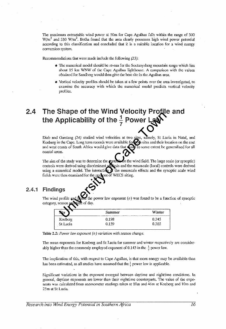
The wind profile and hence the power law exponent (a) was found to be a function of synoptic category, season and time of day.
Site
Koeberg St Lucia
Summer
0.198 0.159
Thble 2.2: Power law exponent (a) variation with season change.
Winter
0.245 0.202
The mean exponents for Koeberg and St Lucia for summer and winter respectively are consider
ably higher than the commonly employed exponent of 0.143 in the .!.. power law. . 7
The implication of this, with respect to Cape Agulhas, is that more energy may be available than has been estimatec,i, as all studies have assumed that the~ power law is applicable.
Significant variations in the exponent emerged between daytime and nighttime conditions. In general, daytime exponents are lower than their nighttime counterparts. The value of the exponents was calculated from anemometer readings taken at lOm and 46m at Koeberg and lOm and 25m at St Lucia
Research into UfndEnergy Potential in SouthernAfrica 16
1
pvf...,,..t,,,hlp wind power at 50m found that the area power 1A',.'-'ll'U<U
""-"l<lUlll;O .... """'.Ull for a wind energy
KecolDIrlendatlorlS that were made
• The nurnenlcal "nv,"".".,ru trlOnOtalln range which lies about 15 km WNW of the """Ulll''''' lilf!hthOllSe. with the values obtame:d. for
• Vertical
The aim of the cotltrols were rlP'·"'~·rI
a numerical modeL The fields were then examined the purpose
The and hence the power law eXlxmenr "<of'p",,",,-,, season and time of
was
Thble 2.2: Power law exl)Onenc (a) variation with season ClIlllI!!e..
to be a
The mean for fi.UIVV""l'.
than the c01DIrlonly p,,,.,n,,,,,,'''' p'''TV'.np"t
summer and winter respec:11
0.143 in the ~ power law.
with to is that more energy may
v<>lUll,au;;'", as all studies have assumed that the ~ power law is ao[)llcable.
are cOIlSider-
v <Uj,a1l,,<::; than
'."/:,"-"'"'''''' variatioIlS in the and conditioIlS. In rt"""hrr,p e;qx)Dents are lower than their The value the expo-
nents was calculated from anemometer taken at 10m and 46m at and 10m and 25m atSt
Univers
ity of
Cap
e Tow
n
Koeberg St Lucia
Day
0.150 0.141
Summer Night
0.246 0.173
Day
0.202 0.177
Thble 2.3: Power law exponent variation with season and time of day
Winter Night
0.286 0.236
Diab concluded that the best estimation of the power law exponent can be achieved by a division of time of day and season for both sites and an added factor of synoptic category for St Lucia
2.5 The Cost of Wind-Generated Electricity in South Africa
The cost of electricity produced by a wind turbine was calculated for various turbines at locations inland and along the coast of South Africa (12) The sites chosen were those where long term wind speed records were available and correspond to the lighthouses along the coast and mainly the airports inland
The purchase cost of the four wind turbines used in the study were taken from a quote from the turbine manufacturers agent in South Africa When this was not possible, the purchase cost was estimated by interpolating between known costs. Transport costs were derived from industry quotes for the cost of transporting the turbine components by sea, rail and road
Installation costs were taken to be 10% of the wind turbine's purchase cost, a figure derived from averaging actual installation costs. Operating and maintenance costs were taken as a fraction of the capital cost This procedure is widely adopted in cost studies and figures of 2 or 3% are used Roberts used a conservative figure of 3%
Although the above procedure follows the pattern of economic studies undertaken by Allen and Bird (23), and South and Templin (26), it is simplistic in the sense that it considers only the installed and operating costs of a WECS. The trend worldwide is to analyse cost in terms of total social cost on a lifecycle basis which means including environmental costs.(51) This would make wind-generated electricity more cost effective than Robert's has calculated
2.5.1 The Cost of Wind Power - Results.
The cheapest energy from the various wind power generating systems considered in Robert's study was 15.6 cents per kilowatt hour from a stand alone system (1983 SA clkWhr). A system which 'stands alone' is one where no energy storage or backup is supplied to supplement power generation when the wind is not blowing. Pumped storage and diesel backup systems were considered, but these raised the cost to 29.7and16.2 c/kWhr respectively.
Robert's results (Table 2.4) show that wind generated power cannot compete in economic terms with conventionally generated power. Grid electricity generated by ESKOM cost 3.47 c/kWhr in 1983, the time of this study. The cost to the consumer was considerably higher, the typical rate being 6.15 c/kWhr, the added amount due to transmission and service costs.
It is important to note that the cost of electricity in remote areas, when connected to the grid, is considerably higher than quoted above due to the high cost of extending transmission wires.
Research into Wind Energy Potential. in Southern Africa 17
Thble
It is irn'l'V\,rt"r,t
Summer
0.177 0.236
law exllOnent variation with season and time
eXIlOnent can be .,,.hip,,,>n
geIleratted {lOwer cannot in economic terms ESKOM cost 3.47
consumer was coIlSldtera,bly traJlSIIUSSlon and service costs.
exl:en1dmg transmission is
Univers
ity of
Cap
e Tow
n
Wind Turbine Wind Speed Energy Cost Station (mis) (c/kWhr)
Port Elizabeth 4.4 15.6 Alexander Bay 4.3 16.0 Cape Town 4.3 16.3 East London 4.3 18.9 Durban 3.2 23.6 Kimberley 3.0 37.6 Johannesburg 3.0 47.2 Pieters burg 2.4 56.8
Tuble 2.4: The cost of wind-generated electricity at nine sites (1983 values, SAcents/kWhr) (27)
Dutkiewicz (50) updated these results to 1989 values and expressed them in USA cents/kWhr. Table 2.5 shows a comparison for Cape Town, one of the more favourable of the sites analysed by Roberts.
Unit Size (kW)
16 265 2000
Cost - USA cents/kWhr Wind Diesel Electricity
14.7 22.7 18.7
29.1 14.5 11.6
8.7 8.7 8.7
Tuble 2.5: Cost of electricity in Cape Town from wind, diesel generation and the national grid (1989 values, USA cents/kWhr) (50)
2.5.2 Sensitivity of Results
In an assessment of the sensitivity of the results, Roberts found these factors of importance:
Enhancement of Wind Speeds
Enhancement of the wind speeds has an inverse linear relationship with the wind energy cost (fable 2.5). A 50% enhancement of the wind speed will produce a 40-50% decrease in the wind energy cost (27) Enhancement of the wind also produces an increase in the reliability of a WECS in meeting a load demand because the shape of the velocity duration curve is changed at the site where enhancement is prevalent
Increase Mean Wind Energy Cost In Wind Speed (c/kWhr) Speed (m/s)
· * A,B,C and Dare the following wind turbines. ref. (28)
A B c D
Model
DVI 15-3 WfS-75 WINDANE29 WINDANE9
Power Law Exponent
Rating (kW)
15 2000 265 16
Type
Darrius Horizontal Horizontal Horizontal
The wind data used by Roberts is recorded by anemometers typically placed at 2, 5 and lOm above ground level. Wind turbine performance curves are functions of the wind speed at the height of the hub of the rotor, which ranged from ll.5m to 80m for the turbines investigated. Roberts used the
t power law to extrapolate the wind speed at hub height. The power law is generally considered as
a conservative measure (23) and, although it may provide reasonable estimates under neutral atmospheric conditions, more power is generally available than would be calculated using an
exponent of+·
The work done by Diab and Garstang (24) showed the exponent to be significantly higher than t for both the east and west coasts of South Africa
Extrapolation of the wind speeds to hub height (taken as 76m) was performed using the power law
with an exponent of 0.15. This is slightly higher than the more often used 0.143 (+).The reason
given is based on information obtained from the Koeberg meteorological tower (24), where an exponent of 0.15 - 0.27 was found to fit, depending on the time of day and season. The use of a
higher exponent than t is valid with a high degree of certainty only for the west coast, due to low
level jet streams induced by transient coastal lows. An exponent of 0.22 would have the effect of increasing the velocity at hub height (80 m) from 9.5 m/s to 11.1 m/s. The corresponding increase in available power would be in the order of 60%.
According to Jury et .. al. (9), the exponent will increase up the west coast and decrease along the south Cape coast due to the destabilising influence of the Cape Agulhas current. At St Lucia on the Natal coast, the exponent was found to range between 0.16 and 0.20. The use of 0.15 is thus considered to be too conservative. The cost of wind-generated electricity as has been calculated by Roberts (12) seems unrealistically high in the light of this, and further investigation into the actual wind profile, under the varying conditions of season and time of day, is warranted.
Reduction of Wind Turbine Costs
The annual cost of ownership and hence the cost of wind power is dependant primarily on the turbine's purchase price. The purchase price is often assumed to reduce as more units are produced, following some 'learning curve' as the development costs are born by a greater amount of turbines. Roberts lists the following- factors that will act against this tendency of cost to reduce with number of twbines manufactured:
• higher design standards • improved safety mechanisms • improved generation systems • higher standards for power quality
The combined effect of these trends leads to uncertainty as to how the cost of turbines will be affected in the future and how this will in turn affect the cost of power generated
Research into Hind Energy Potential, in Southern Africa 19
*
A B C D
and D are the 'VlllVVY'~ wind turbm:es.
Model
DVI 15-3 WfS-75 WINDANE29 WINDANE9
15 2000 265 16
Power Law _ .... _ .. __
work done
at 2, 5 and 10m above at the the
l.A>Lll5""'1.A.I. Roberts used the
"nr,Ul"" the PY,"'npnt to be SlglrnllcarlUy
an
1 1
as was the power law
than the more often used 0.143 ( The reason
on information obtained from the "'''\.J'\A.)'\~."" me:teo.roIQglcal tower (24), where an "'VT",,,.,,,,,.,t of 0.15 - 0.27 was to and season. The use of a
1. is west to 1
eXllOflient will up the west coast and decrease the u='laIJ'lll"lll!:;influence of the current. At St Lucia on the
pVTV\npnt was to range between 0.16 and 0.20. The use 0.15 is thus too conservative. The cost of as has been ................ 0." ...
in the "'""U!5'''<VU into the actual conditions season and time of
Reduction of Wind Turbine Costs
wind power is on the is often assumed to reduce as more units are pro-
..... WlUll"5 curve' as the costs are born amount of that will act this ren(lem-;y
with number of twbines manufactured:
The combined aU (::cte~d in the
these trends leads to ",.",,,,ri.,,
and in turn power gel1lerated.
Univers
ity of
Cap
e Tow
n
At the time of Robert's study it was assumed that all the turbine components would have to be imported Diab (29) has estimated that if all the components, except the blades, were made inside South Africa, this would halve the capital oost. The capital cost could be even further reduced as the technology used overseas for constructing the blades, the spun epoxy graphite process, is now used locally in the boat-building industry. These factors could provide a significant reduction in the estimated cost of wind-generated electricty.
Cost of Grid Electricity
The ability of wind-generated power to compete with grid electricity in the future depends to a large degree on the rate at which utility power cost escalates. Using the rate of increase for the 10 years prior to 1983, and projecting the cost over the life of a wind turbine (20 years), Roberts found that ESKOM power would be well below the cost of wind-generated power. It is important to note, however, that these projections were made before the era of financial sanctions, and the rapid decline of the Rand soon after 1983. The cost of grid electricity has risen sharply as a result, especially the domestic tarriff.
There are also significant implications for remote areas which are some distance from the existing grid The cost of extension of high voltage power lines to isolated villages, clinics, schools and towns is often prohibitively expensive. It is in these areas that wind power may be competitive with grid power.
Three factors thus arise from the sensitivity analysis which would have potential to reduce the calculated cost of wind power significantly:
· • Enhancement of the wind regime will yield higher values of available power than calculated by Roberts.
• The assumption that the~ power law is applicable, yields significantly conservative
velocity estimates
• The capital cost reduction that would be likely to occur if wind tUibines were produced locally
Further investigation into these criteria is required to improve the estimation of the cost of wind-generated electricity in South Africa.
Research into Jttnd Energy Potential in Southern Africa 20
of Grid 11;lf'rtl~lrl
There are
power.
Three factors
• m!1an,ceIIlent
remote areas power
It is in these areas
• The ""~'lll"IJLJlVU that the t power law is alJl.Ju~..aVjl"',
• would be to occnr if
requm:a to
the
turbines were prCKlu<cea
the cost
Univers
ity of
Cap
e Tow
n Chapter 3 The Methodology of the Study
The Methodology of the Study 21
Univers
ity of
Cap
e Tow
n
3.1 Site Selection Procedure .
3.1.1 Regional Analysis
The research into wind energy in South Africa (described in Chapter 1\vo) shows that the coastal belt, in particular the southern and western Cape, exhibit good potential for using wind energy.
\
The Cape Agulhas region was chosen for a model siting study, carried out by Botha in 1988.(10) The series of hills that were modelled and tested showed enhanced wind speeds of 5% to 10% above those measured at the lighthouse. These hills, the Sandberg, rise to a height of 156m above sea level and lie just inland of the village of Cape U Agulhas.
3.1.2 The Soetanysberg - A possible WECS site
Botha recommended that a further study in the Agulhas region be carried out ..
Aerial photographs of the coast east and west of the Sandberg showed that the Soetanysberg, 15 km to the west of Cape Agulhas exhibits good potential for velocity enhancement The smooth rounded shape of the mountain (height =262m) would minimise turbulence and probably create regions of relatively high velocity.
Figure 3.1: Three dimensional projection of the Soetanysberg
It can be seen that the general orientation of the mountain is along an E-W axis. This is the same direction as the prevailing winds (WNW, W, WSW, ENE, E, F.sE). If the wind-stream split around the sides, instead of being forced over the top, little or no enhancement would result. The mountain, however, is approximately ten times wider than it is high and this, combined with the relative smoothness and rounded shape, makes it a good possibility for a WE.CS site.
3.2 Current Site Assessment Techniques
Experience with wind turbines has indicated that one of the most important factors controlling the success or failure of these systems is site selection. The incorrect siting of a wind generator by a few kilometers can drop the performance by 20% of the original expectations. (30)
7he Methodology of the Study 22
1
1.1
1
recommended that a
3.1: Three dirnpr,~irm
It can be seen
is "PlJHJ.lUU''''',l)
relative smoothness and "I"\"nn~'n
wind twbines has mdlCaJted success or failure of few kilc)meters
be carried out.
coastal energy.
the ~ole[aJnvs.oeJrg.
aWECS site.
a
Univers
ity of
Cap
e Tow
n
Operating experience in Altamont Pass, California, shows that energy production drops in the order of 40% are found between rows of turbines 300m apart. Thus it is important to find a suitable site that exhibits the highest wind speeds, relative to the surrounding area. The more accurately the siting can take place, the lower the overall power production costs will be.
A number of site assessment techniques were investigated as possible options to determine the best site in the Agulhas region. These are explained and their relevance to this study is discussed in the following sections 3.2.1to3.2.4.
3.2.1 Ecological Surveys
F.cological swvevs are based on the examination of eolian (wind-blown) landforms or the deformation of vegetation due to the prevailing winds. This method is useful in that it can be used to rate various sites in order of merit, as well as provide direct estimates of the long term mean annual velocity.
Some of the index values that are used to relate deformation to wind speed are easily obtainable.
At Cape Agulhas, however, the ground cover is mainly Fynbos. Analysis of the deformation due to the wind would require special equipment and laboratory testing. Ecological swveys are also not suitable when trying to establish the true enhancement in a small area This method is therefore suitable for obtaining a comparison of various sites, but cannot be used to predict the wind speeds accurately.
Figure 3.2: A wind deformed tree showing the prevailing wind direction
3.2.2 Direct Wind Measurement
The data obtained through direct wind measurement is the most obvious way to assess the wind energy potential of an area
Over large areas, however, it can become a very costly and time-consuming process, but has been used in some investigations (31, 32). To obtain an accurate wind speed distribution, or average annual wind speed, it is necessary to monitor the winds for at least a year.
If long term measurements are not feasible, it is possible to use statistical methods to estimate long term wind speeds at a site, provided there are long term data for another site in the region. (33)
There are various methods that can be used to physically measure the wind velocity. Some of these are outlined below.
Doppler Acoustic Sounders
This is a sophisticated method of sampling wind speeds. A sound wave is transmitted into the atmosphere and reflected back by particles being carried by the wind The doppler shift in the reflected sound wave is used to calculate the
1he Methodology of the Study 23
1
to determine the best IS in the
rate various sites in term mean
values that are
obtlliniIlg a coIlnparis(ln cannot be used to
3.2: A wind nof"""Ylon nN'VlI,llltiIO wind direction
The data obtained thrIDll,!l;h wind measurement is the most vv,"v • ..., way to assess wind energy PU',"'llIL1<U of an area
Over it can become a very and tin:le-(;onsurwng process, but has been To obtain an accurate or average
it is necessary to monitor the winds for at least a year.
If term measurements are not """""UI", term wind at a
There are various methods that can be used to nh1J!':11::a1JlV measure the are outlined below .
...... ," .... '." Acoustic Sounders
This is a 1>UljH"'U"'4L~;U
Some of
Univers
ity of
Cap
e Tow
n
the wind speed The equipment is cumbersome and has to be carried on a motor-vehicle trailer. It can therefore only be used in areas accessible by motorcar. Only two accoustic sounders were to be found in South Africa and neither was easily available.
Tethered Meteorological Balloons
Anemometers with transmitters, or self-recording devices, can be hoisted by a tethered balloon to the height of interest and readings taken. Tethered balloons are used extensively for low velocity sampling, but at wind speeds higher than lOm/s they tend to get drawn down in a lazge arc by the wind The method is unsuitable for wind enetgy studies where the wind speeds of interest are in the 5 to 20 m/s range.
Untethered Meteorological Balloons
This method involves the release of an untethered balloon which is tracked using optical or electronic methods. The rate of ascent, i.e. the vertical component of the tracked velocity, is a function of the relative buoyancy of the balloon to the atmosphere, and can be calculated The horizontal wind speed is then calculated by closing the vector triangle.
Untethered balloons require complex electronic distance measurt'.ment, or at least two observers using trigonometrical surveying techniques to plot the path of ascent. The technique is not well suited to monitoring the velocity gradient above a specific point, as the balloons get blown downwind and away. from the site as they rise. The measurement of gusts (and therefore turbulence) is not possible with this method
Kite Anemometry
The use of kites to raise self-recording meteorological instruments dates back to the turn of the century. Due to the weight of the measuring instruments and either the recording or transmitting device, powerful kites are required The method is generally cumbersome and time-consuming, although compared with balloons, the instrument lifting component is simpler.
A recent development has been the Tethered Aerodynamic Lifting Anemometer (TALA).
The TALA was designed and made as a simple, lightweight, portable alternative of velocity measurement to the methods described above. In principle the system is a small, lightweight kite, attached to a calibrated spring balance with non-stretching kevlar line. The kite is made of JYvek, a plasticised paper. It is manufactured by Dupont and is especially designed for stability in high winds. The design is a small version of the Scott Sled and can be flown in winds from 4 mis to 20 m/s.
The kite itself with tail has been calibrated by the manufacturer in the United States National Bureau of Standards as well as the NASA-Langley wind tunnels. Independent testing has been carried out by a recognised journal (34 ), by flying the kite alongside anemometer masts. The accuracy was found to have an error of 2.5%. The manufacturer claims a 2 % error in both direction and wind speed
TALA Kites were used successfully in the siting of fifteen 600 kW wind turbines on the island of Oahu in Hawaii. The predicted power outputs have been found to correlate closely with the output under operating conditions.
The Methodology of the Study 24
car. was
Tethered etel()rOltlgllCal Balloons
Untethered Me'te(Jlrologi:cal Balloons
then ""-'''WlaL'''''
site as rise. The measurement pos;slble with method.
Kite
IS
A recent ..,lVl-'lll..,lll has Anemometer
The TALA was ae~;IgIlea and made as a measurement to the me:tI1(Xls
attached to a calibrated
manufactured and is in The is a small version of the Scott Sled and can be flown 4 m/s to 20 m/s.
The kite with tail has been calibrated by the manufacturer in the States National Bureau of Standards as well as the wind turl-
has been out a '''''''''Vh'U''~'U alongs;lde anemometer masts. The accuracy was found to have
The manufacturer claims a in both and
TALA Kites were used in the bines on the island of Oahu in Hawaii. The nrp£lIrtp.f1
found to correlate with the
Univers
ity of
Cap
e Tow
n
3.2.3 Numerical Modelling
This method is becoming increasingly popular for screening areas for possible wind turbine sites because of the speed with which the analysis can be carried out All numerical models require historical wind data for at least one site in the region. These are then used to predict wind velocities at any other point with respect to the particular terrain characteristics.
There are two basic types of numerical models, wJrlch can be classified as: • objective-analysis models • primitive equation models
Objective-analysis models use observed wind vectors from a number of stations to interpolate the wind over a region according to the constraints imposed by terrain and the equation of continuity. The model requires a number of simultaneous observations, between 7 and 30. However with insufficient wind field data it contains little to define the flow and performs poorly. (13)
Primitive equation models take account of the mesoscale effects of orography, friction and heating on surface winds and hence are capable of simulating orographic channelling, land and sea breezes and anabatic and katabatic winds. They require very few input specifications and are ideally suited to data sparse regions containing complex topography.(13)
The Energy Research Institute has access to an integrated numerical model designed specifically for the siting of WECS. The programme is made up of five distinct sub-models as follows:
• Roughness Change Model • Shelter Model • Orographic Model • Windatlas Analysis Model • Windatlas Application Model, ·
The programme is called the Wind Atlas Analysis and Application Programme (WASP), and was written by members of the Department of Meteorology and Wind Energy at the Riso National Laboratory in Denmark. It is sponsored by the International Energy Agency and has been verified by field tests carried out by the IEA.(17) It is widely used throughout Europe for the siting of WECS.
3.2.4 Physical Modelling The use of wind tunnels to assess the wind energy potential of an area is an accepted and well-documented technique of analysis. 1\vo approaches can be taken. The one is site-specific, where a physical model of the proposed WECS site is used to find the region of maximum enhancement(35) The other concentrates on generalised hill shapes under various flow conditions, in order to establish generalised solutions for airflow over hills.(36)
3.3 Method Adopted for Site Assessment
The availability of the WASP computer programme, its ease of application and the relatively low cost of using it, made it the obvious choice for analysis. The use of a direct measurement technique (such as anemometers, kites, etc), or of physical modelling would have been more time consuming and expensive.
Chapter Four gives a detailed description of the model and how it was used to analyse the wind patterns in the vicinity of the Soetanysberg.
The Methodology of the Study 25
access to an int!!gr.:lted nmnerlcaJ. WECS. The progrnmme is made up
• Kolugtmess '-',LI£U-'!".v
•
progrnmme is called the Wind Atlas members the Depru1ment
<l1v>r<lt""" in Denmark. It is SpoUSQlred
the WECS.
wind energy of an area is an and Tho can be The one is Sl[f~-s):leC1nc,
Pro1PQsc::d WECS site is used to find the The other concentrates on hill
to establish
GV<lWaJUU..I.J of the WASP progrnmme, its ease of and the "",,,,"v'plu
it, made it the obvious choice for The use of a direct measuremen1."""LUll',!Uv
'-'ll<llA'W Four pattenlS in the
or of have been more time COIISUlntIllg
a detailed d.eS,cn1Pb()n of the model and how it was of the :Sm~tarJlvstlerg
to '"'''' v"r; the wind
Univers
ity of
Cap
e Tow
n
3.3.1 The Need for Validation of the Numerical Model - WASP
The accuracy with which the wind power for a particular site can be predicted depends on how closely the mathematical equations reflect what is actually happening. Experience from windparks elsewhere in the world show that the model predictions of the available energy did not always correlate closely with the values obtained after the turbines had been erected
The investigators of a Greek wind farm park found relative wind speed errors between a wind tunnel model and measurements of 3 to 8%(38) Numerical modelling, used in the same study, produced errors between 4 and 13% Field tests conducted in Denmark on the flow model used by WASP (the BZmodel) have shown a high degree of accuracy.
WASP has previously been compared with a physical model tested in a wind tunnel.(10) The comparison showed that both models predicted wind enhancement to within a few percent of each other. In order to be certain that WASP was being used correctly and that the predicted velocities were accurate, it was necessary to measure wind speeds on site and then compare these with the model.
3.3.2 Method Adopted for On-Site Measurements
The field measurements required for validation, had to include the full range of heights at which WASP predictions would be made. When calculating the predicted power output of a wind turbine, the velocity at the hub height of the blade is used This study, however, is not concerned with any specific turbine, so allowance had to be made for all possible heights of interest The hub height of wind tutbines ranges from lOm tolOOm above the ground The tip of the blades, however, could intersect the air stream up to 150m a.g.l.
The need to validate WASP in this region left few choices of velocity sampling, and it was decided to use the TAIA kite for the field measurements. It was found to be the least expensive, most portable and fastest way of measuring wind velocities in the range required
The experimental method used to collect wind speed data at selected sites on and around the Soetanysberg is described in detail in Chapter Five.
The Methodology of the Study 26
1
WASP has tested a fJ." ...... "'L"' ... wind enhancement to within a
the pr(!(:I1cteXi VC!iOclbes
on the '-llalJl1(;;. Five.
Univers
ity of
Cap
e Tow
n Chapter 4 Siting Analysis Using the Numerical Model - WASP
Siting Analysis using the Numerical Model 27
Univers
ity of
Cap
e Tow
n
4.1 Introduction to WASP
The Wind Atlas Analysis and Application Programme (WASP) is a programme for the horizontal and vertical extrapolation of wind data
In a general way it takes into account the effect of different roughness conditions, sheltering effects due to nearby buildings and other obstacles, and the modification of the wind imposed by specific terrain characteristics. It provides the user with means of correcting the basic meteorological data, as well as offering the tools for detailed siting of wind turbines. It is currently being used in some European countries in their wind energy siting programmes.(17)
WASP requires a detailed description of the following:
• The shape of the topography and coastline surrounding the site in the form of a c,iigitised map.
• The surf ace roughness conditions of the area surrounding the proposed site. • The shape, size and orientation of any obstacles near to the proposed site. • Historical wind data for a point within the digitised area • An operating cwve for a wind turbine if the absolute energy in kW is to be calculated.
When all of this information has been entered into the computer, the wind speed (mis) and energy density (W/m2) at any point is found by specifying the new site (with X and Y co-ordinates) and providing the roughness and obstacle description for the new site. By changing the height of calculation a vertical velocity profile can be obtained for any point within the area.
4.2 Topographical Description
In order to calculate the wind velocity perturbations induced by orographic features such as single hills or more complex terrain, WASP utilizes a modification of the Jackson and Hunt themy for flow over hills, which was developed for the specific purpose of detailed wind generator siting.(39)
The orographic basis for the complex terrain flow model of WASP is a digital height contour map. The terrain described in this may be' real' or an idealised Gaussian hill that can be created by WASP.
The shape of the Soetanysberg was not easily described by a Gaussian hill so a 1:10 000 orthophoto map was traced and digitised. The height of each contour was specified and the X and Y co-ordinates were generated by a digitising tablet at the Department of Land Swveying of the University of Cape Town (UCT). To obtain values from the tablet, a short computer programme had to be written. The map was larger than the digitising tablet so the programme incorporated a routine to adjust for a shifted origin. The programme listing can be found in Appendix II.
WASP specifies a maximum of 10 000 co-ordinate pairs that can be digitised. Only 20m contour inteivals were traced out to prevent the limit being exceeded The area that was digitised was defined by 9800 co-ordinate pairs. These data points were formatted to WASP specifications and stored on floppy disk as well as on the Speny mainframe computer at UCT.
Plots of the digitised points shown in Appendix ill.a, were generated using the Saclant Graphics Package on the mainframe. The contour map of digitised points (Appendix ill.b) compares well with the map produced by the Swveyor General (Appendix m.c) which is conf"mnation that no errors were made in the digitising process.
Siting Analysis using the Nwnerica/, Model 28
1 I .............. ". ........
• map.
The
is a programme
tOJX>graphy and coastline SWTiOUD(Jmg in
a Gaussian bill so a 1:10 000 X and
can 20m contour exc:eeclea. The area was was
tOfiMttl~toWASPs~arl~.ous
mal.ntntme coDlputer at UCf.
Univers
ity of
Cap
e Tow
n
4.3 Roughness Classification
The roughness of the terrain surrounding a site is determined by the size and distribution of 'roughness elements' such as vegetation, built up areas and the soil surface. The geometry and physical characteristics of the various roughness elements are the parameteIS that determine the roughness length zo (zo is the height where the mean wind speed becomes zero if the wind profile has a logarithmic variation with height - see section 1.3.2)
WASP specifies a descriptive and illustrative technique whereby four roughness classes are def med and roughness lengths are attached to these. The descriptions are given below.
Roughness class 0 - Water Areas: the sea, fjords and lakes
Roughness class 1 - Open areas without significant windbreaks. The terrain appears to be very open because there are only very few wind breaks, if any. The terrain is flat or very gently rolling. Single farms and stands of low bushes can be found
Roughness class 2 - Farmland with windbreaks with a mean separation in excess of lOOOm and some built up areas. The terrain is characterised by huge open areas between the many wind
. breaks, giving the landscape an open appearance. The terrain may be flat or strongly undulating. Trees and buildings are common.
Roughness class 3 - Urban districts, forests and farmland with many windbreaks. The farmland is characterised by the many closely spaced windbreaks, the average separation being a few hundred metres. Forests and urban areas also belong to this class.
The description of the terrain and the choice of the roughness lengths is subjective; therefore different results may be obtained by two useIS performing the same analysis. The shape, and to some extent the magnitude, of the velocity gradient depends on the roughness of the surface. The accuracy of the description is therefore important Figure 4.1 shows the effect that changing the roughness length has on the shape and magnitude of the velocity profile.
18
16
14
10
0 20 40 60 80 100 Height a.g.I (m)
Figure 4.1: Effect of roughness length on velocity profiles.
Siting Analysis using the Numerical, Model
- Zo • 0.01
Zo • 0.06
---· Zo • 0.2
a Zo • 0.4
120 140 160
29
Rolllgtlne:ss class 0 - Water Areas: the sea,
18
16
14
12
10
o 20 40 60 80 100 120
Zo • 0.01
Zo·O.OI5
2:0·0.2
Zo • 0.4
140
are
U;U'LUU""U is
160
Univers
ity of
Cap
e Tow
n
On completion of the field tests using the TAI.A kite, it was possible to make the model more accurate by adjusting the roughness descriptions so that it yielded more realistic results. The roughness of the Fynbos, the predominant cover, was taken as 0.04 in the final analysis.
The roughness of the area has to be described for each possible WE.CS site. The point being investigated forms the centre of a circle of 5 - 10 km in diameter. The roughness characteristics of each of the 12 sections within the circle are then described according to the terrain type. Changes of roughness lengths can occur a number of times within a given sector where required
No obstacles were used in the site analysis, since the terrain being investigated was open land with no major obstacles.
4.4 Historical Wind Data
The historical wind data records, recorded by the Weather Bureau at the Cape Agulhas lighthouse, were obtained by Botha in 1988. The records, which spanned six years, were mganised at the time into a format that WASP could use and the same data files were used in this study.
The raw data used by the numerical model requires that an anemometer height be entered in order to establish a reference height for the historical data. The height and also the exact location where the wind speed is measured at Cape Agulhas is questionable.
Diab uses an anemometer height of 5m above ground level and normalises an average wind speed of 6.5 m/s to 7 .2 m/s at lOm above ground level. On visiting the lighthouse at Cape Agulhas in June, 1988 it was found that a new anemometer on a 5m mast, with a tape recording data capture system, had been installed One year later, however, this anemometer was not operational, and according to the lighthouse-keeper, had never been utilised The wind speeds were still being recorded by the lighthouse-keeper using the Beaufort Scale (Appendix IV). Botha states that the Weather Bureau Office at DP Malan Airport in Cape Town periodically cross-check the values recorded by the lighthouse-keeper.
Botha decided to use approximately the same value as Diab calculated as the reference wind speed (ie. 7.2 m/s at lOm above ground level). An anemometer height of 2m was chosen so that WASP yielded the same wind speed at lOm as Diab obtained
On intetviewing the lighthouse-keeper, it was found that the Beaufort Scale was applied to the condition of the sea in the vicinity of the lighthouse and as such all measurements made were relevant to a location about 50m off the shore and not to the location of the anemometer mast just in front of the lighthouse. On this basis analysis of the wind speeds was carried out using a point 50m offshore in a southerly direction as a reference point for the wind data. The reference height was chosen as 2m. This procedure affected the calculation of the 'wind atlas' for the Agulhas region, which is the geostrophic flow calculated by WASP from which the site-specific velocity predictions are made.
It is important to note that while there is uncertainty attached to the true value of the mean wind speed at Cape Agulhas, the frequency at which the wind blows at various sectors is known. The percentage change in the wind speed due to the topography will not be affected by the uncertainty, only the predicted average at that site.
Siting Analysis using the Numerical Model 30
m
the TAlA
the
same as An anemometer
at 10m as Diab obtained
ommolre In a SOllth(~rly \JJ.1~Iu.u was chosen as 2m. This oroced.ure att(~tf:d
which is the flow call~llliltf:d 1-" ......... '-UV1Jl.:> are
'""'~'lI".aLVU was open
there is attiilclllea to the true value of the mean t.",.,."",,, ... , at which the wind at
due to the topograpllY
Univers
ity of
Cap
e Tow
n
4.5 Experimental Procedure Using the Numerical Model , ·
All of the data that the progranime required was stored on disk. A square grid was imposed on the map using the same co-ordinate system as for the digitised map.
The grid points were taken at intervals representing a true distance of 500m apart so that the terrain was described by a total of 250 grid points. The origin of the grid was chosen to lie on the coastline at the following co-ordinates:
Latitude: 34° 46' 03" Longitude: 19° 51' 00"
The borders of the digitised area have ~e following cartesian coordinates:
Western border: Longitude: Eastern border: Longitude:
34° 43' 5" 34° 47' 47"
19° 46' 24" 19° 56' 00"
The digitised map and the wind-data files were then entered into the programme. The site was specified by X and Y co-ordinates and a terrain-roughness file corresponding to the site was entered. By specifying the height above ground level and invoking the calculation procedure, the model calculated the wind speed and energy density for the site. The wind speed and energy density were calculated for 20m, 50m and lOOm above ground level at each site.
In order to improve the resolution in areas where acceleration of the wind stream occured, the grid was refined to a true distance of 250m apart. This enabled the regions of highest wind speed to be located more accurately.
Siting Analysis using the Numerical, Model 31
that the prograDin:le re;quiredwas stored on
The borders
Northern Southern
Eastern
46' 03" 51' 00"
as for the map.
chosen to lie on
dlJ!;lW.ed area have ~e tnll!nwina ....... ,..., ....... c<xm:JJinaites:
43' 5" 47' 47"
46' 24" 56'
Univers
ity of
Cap
e Tow
n
,.
Chapter 5 Validation of WASP by Comparison with Field Data
'
Val.idation of WASP by Comparison with Field Data 32
Univers
ity of
Cap
e Tow
n
5.1 Experimental Method
Predictions from the numerical model (WASP) were compared with actual measurements from the field to obtain an indication of how accurately the model simulates reality.
The procedure that was initially adopted is listed below:
• The wind was to be measured at five points on and around the Soetanysberg.
• Hourly velocity readings were to be obtained from the Cape Agulhas lighthouse anemometer over the time period that the TAIA kite was flown on the Soetanysberg.
• The lighthouse anemometer readings were to be used as input to the numerical model and the predicted values compared with those measured on site.
On arriving at the lighthouse it was found that the rotating cup anemometer on a Sm mast was not working. The lighthouse-keeper, who was in charge of the digital equipment, had no need to repair it. He was certain that the Beaufort Scale which he had been using for the past 35 years was as good as the anemometer which, in his opinion, was badly placed with regard to the lighthouse buildings.
Due to the necessity of obtaining accurate data, a TAI.A kite was used at a position on the coastline due south of the lighthouse to obtain the hourly data to be used as input for WASP. This reference kite was flown at lOm above ground level.
A preliminary analysis of the wind flow over the Soetanysberg was performed using WASP. This yielded certain regions of relatively high wind speed Four points were chosen in these regions as sites for the field tests (Sites A,B,C and D). One other point (Site E) on the coastline towards the western end of the Soetanysberg was also chosen as a site. This allowed for a comparison to be made of a site that was not affected by orographic forcing. The locations of the field-test sites are shown in Figure 5.1.
Site C
N aq:
. Figure 5.1: Map ofthe Soetanysberg with the sites where the 'E4IA Kite was flown
Validation of WASP by Comparison with Field Data 33
1
measurements from
adclpte:d is listed
• The wind was to measured at
• ane-was
real:nns~s were to be used as colnpared with those measured on
to numerical model
cup anemometer on a 5m mast was not
western end made of a site that was not att!!cted
5.1.
:V);'rmrl'\J~'nplrQ with the sites where the 1AIAKite
no to 35 years was as
to
Univers
ity of
Cap
e Tow
n
The field measurements on the Soetanysberg were undertaken using a second TAIA kite. The heights at which wind speeds were sampled were 20, 50, 80, 110 and 150 metres above ground level. Velocity profiles were also measured in front of the lighthouse where the reference TAIA kite was being flown.
The two prevailing wind directions are the easterlies (mainly summer) and the westerlies (mainly winter). The field measurement took place in both of the prevailing winds.
5.2 Instrumentation
The kite anemometer utilises a spring-mounted disc within a 28 mm plexiglass tube moving along a wind speed scale calibrated in miles per hour. The spring is attached to one side of the disc and the kite line to the other. The spring was calibrated each day before and after the measurements were taken, by banging a 500 gram weight and adjusting the scale to read 19.8 mph as recommended by the manufacturer. (40)
The kite line is made from non-stretching Kevlar line which transmits the wind felt by the kite face, without any damping effect. Turbulence is measured very effectively in this way.
The kite altitude was calculated from the corrected line length multiplied by the sine of the elevation angle. The line length was marked on the string and a correction factor of 0.95 was used to account for the catenary sag. The figure of 0.95 was recommended by the manufacturer (41) and used by Daniels. (33) The elevation of the kite was measured using an inclinometer supplied with the system. Since the kites sometimes flew above hills with the measuring unit located downslope or upslope, it was necessary to compensate string length for the height difference.
This was done using the following expression:
H = Cr L [ sina - cosa tanB] [Eq 6] H = height of kite above ground level Cr= catenary sag correction factor ( = 0.95) L = actual line length a = kite angle B = angle to point on hill directly below kite
,, /
/ /
--/
/
,/ L
--
H
Figure 5.2: Ki.te flying above hill, showing variables for height calculation
Validation of WASP by Comparison with Field Data 34
Velocl.'Lv orotilles were
is nOIl-stretC::IWl2 Kevlar Tw:bnllem:e is measured
was done the toU.OWUlIl exr:n:es:sion:
--13
above
'" '" L
--
rI' .... ,.,.,.m below kite
westerlies
H
Univers
ity of
Cap
e Tow
n
5 .. 3 Measurement Procedure
5.3.1 Soetanysberg Readings
The sites were located by using the swvey technique of intersection. The two trig beacons and two markers acted as reference points for the swvey.
Velocity readings were taken at 20, 50, 80, 110 and 150 metres above ground level. Forty readings at 10 second intervals were taken at each level on the ascent as well as the descent of the kite. Due to the twbulence of the wind, the spring and marker disc were constantly moving. To minimise the bias that could occur from visually averaging, the line was 'grabbed' at the exit point of the calibrated tube at the 10-second interval and the reading taken. The average velocity and the standard deviation were calculated and noted before moving to the next height The entire sample took an average 90 minutes to complete. The time of day was noted at the start and finish of each sample.
5.3.2 Lighthouse Readings
The ref cience kite which was flown on the coastline due south of the lighthouse was read using the same 'grab technique' as described in 5.3.1. The height chosen was a constant lOm above ground level. Each hour, 50 readings were taken at 20-second intervals. The average velocity and standard deviation were then calculated.
Validation of WASP by Comparison with Field Data 35
two two smvey.
Univers
ity of
Cap
e Tow
n Chapter 6 Presentation of Results
Presentation of Results 36
Univers
ity of
Cap
e Tow
n
6.1 Comparison of Model Predictions with Observed Values
6.1.1 Presentation of Results
A typical graph of the velocity profiles measured with the TALA kite and predicted using the WASP numerical model is shown in Figure 6.1. The full set of graphs is found in Appendix V.
Figure 6.1: Example of predicted vs observed velocity profile
Velocity profiles were measured at a number of the sites in both west and east wind conditions, while some of the sites were only sampled in one wind direction. Velocity was measured on the ascent and the descent, hence the two points for each height sampled For ease of discussion an abbreviated form of reference will be used to refer to the site and wind of interest. This will be as follows:
• Lw - Coastline due south of lighthouse in a west wind • Le - Coastline due south of lighthouse in an east wind • Aw - Site A, west wind • Ae - Site A, east wind • Bw - Site B, west wind • Be - Site B, east wind • Cw - Site C, west wind (not measured in east wind) • Dw - Site D, west wind (not measured in east wind) • Ee - Site E, east wind (not measured in a west wind)
6.1.2 Statistical Procedure
For each set of data (modelled and obseived velocity profiles), the correlation co-efficient (r) is used as an indicator of how well the obseived and modelled winds agree height for height. In other words, r indicates how well the model predicts the shape of the velocity profile.
The statistic: t = r [ (N-2) I (1-r2) ]0·5
where N is the number of pairs of records used to calculate r, has a student's t-distribution with N-2 degrees of freedom and is used to test the following hypothesis (the statistical procedure of Daniels (43) is used). N =400 for all sites sampled
Presentation of Results 37
1
1
1
1a.-----~----~----~----~----~----~----~-----.
16
14
12
10 "
8
lIghthouae, Westerly
Kite Observations
6~--~--~--~--~--~~~~~~~~ o 20 40 60 80 100 120 140 160
6.1: l!.:Ktl111lJ1 e
the
COIldltlODlS, while
• Lw - '-A/.""uu • ..., due south of liglh.tholliie in a west wind • Le - due south in an east wind
west wind east wind
measUIed in east measured in east
measured in a west
For each set of data and obsetved used as an indicator of how well the obsetved and modelled winds agree
r indicates how well the model the of the "p,,,,..,',",,
The statistic: t = r [ /
where N is the number of of records used to calculate r, has a student's N-2 of freedom and is used to test the
IS N =400 all sites ,,<U,,~."..., .....
Univers
ity of
Cap
e Tow
n
The hypothesis (H1) is: r is significantly greater than zero, thus a one tailed test is used.
Statistical tables were used to give the probability of at-value as great as t. If this probability is named Pr, then for a given number of degrees of freedom, the following limits.can be defined and conclusions made.
• If Pr >0.1, r is not significantly greater than zero (NSG) - reject H1 • If 0.1>Pr>0.01, r is probably significantly greater than zero (PSG) - accept H1
conditionally • If Pr< 0.01 then r is significantly greater than zero (SG) - accept H1 unconditionally
Another measure of accuracy is the parameter m: m = [ 100 (Vo- Vm)] /Vo
where the subscripts o and m denote obsetved and modelled values respectively, and Vis the average velocity. The m parameter is used as a measure of how well the modelled and observed means agree.
6.1.3 Discussion of Results
Visual examination of the velocity profile plots (Appendix V) shows that the modelled and observed winds agree well. The correlation of the profiles (plotted in Figure 6.2) is good except for one site, Ae (Site A, east wind).
Correlation Coefficient (r)
0.8
0.6
0.4
0.2
0 Lw Le Aw Ae Bw Be Cw Ow Ee
Sites Compared
Figure 6.2: Correlation coefficients of observations vs predictions
The reason rat Ae is so low is that the observed values are at some heights above the predicted values and other heights below the predicted values (see Appendix V). If the correlation is performed up to the llOm level, it yields a value of r equal to 0.701, which is good This shows that the shape of measured profile at Ae is modelled well up to llOm, but is not accurate up to 150m. It is noteworthy that although the shape of the modelled profile has a relatively low correlation, the average accuracy of prediction for that site is within 6.5% of the obsetved values. The worst estimate was at the 20m level where the velocity was underestimated by 14.6%
Figure 6.3 shows them parameter averaged over all heights, as well as the greatest value (and therefore worst prediction) at each site. The average error of all sites and all heights was found to be 7.0o/o, with a maximum error of 15.4%.
Presentation of Results 38
1
The hyplOthlesis IS: r IS sl$.!;lmllcarltlv than zero, thus a one tailed test is used.
• If Pr< 0.01 then r is 31!';llUJ'\.4JLlUy
Another measure accuracy is the ",o,,""'rr,pt,>r m:
average means agree.
0.8
0.6
0.4
0.2
o
Correlation Coefficient
m := [100
modelled values res)JeCtlvel V is the well the modelled
shows that the Ill'U'""""",,,,, is
Lw La Aw Aa Bw Be Cw Ow Ee
Sites Compared
6.2: Correlation
the average accuracy The worst estimate was at the 20m level where the
above the pre:dic:ted If the correlation is
This shows
n"""rr,pt,>r "'JPr"""f1 over all as well as the arp,,,tpd value therefore worst at each site. The average error of all sites and all was found to
with a maximum error of
Univers
ity of
Cap
e Tow
n
Error (%)
20
15
10
6
Lw Le Aw
- Maximum Error
~ Average Error
Ae Bw Be Cw Ow Ee Sites Compared
Figure 6.3: Average and maximum prediction error
At all the sites except Aw, the 20m value is underestimated It was thought that this may be due to an error in describing the site roughness, but adjustments in the model had the effect of shifting the whole profile up or down (relative to the observed values), rather than affecting the lower heights only.
Figure 6.4 shows the percentage of modelled winds above or below the measured winds for both the west and east wind conditions. The model results show a consistent underestimation of the velocity when compafed with the east wind measurements. The west wind predictions were however slightly more often overestimated.
(East Wind) (West Wind)
Below 46%
: :. . ·.
~• .. , ·. Above 54%
Figure 6.4: Percentage of predi.cted results below observed values
1bis indicates that the model tends to be on the conservative side when predicting wind velocity.
Presentation of Results 39
Lw Le Aw Ae Bw Be Cw Ow Ee
6.3: AU,,·rnc.p matimum oretUclrlon error
Below 46%
below observed values
This indicates that the model tends to be on the when Drt:dl(WlS! wind
Univers
ity of
Cap
e Tow
n
The shape of the WASP profile is in closest agreement with the modelled profile in the 50 to llOm range. The hypothesis Ho is unconditionally accepted for all sites at the highest degree of significance except at site Ae. Table 6.1 lists the statistics.
Tuble 6.1: Statistics for comparison of observed and predicted values
6.1.4 Comparison with Other Models
A direct comparison of modelled results is frequently not possible due to differences in scale and site specification. 1\vo other model studies, however, will be discussed to compare the quality of the results obtained in this study.
The first is the physical model analysed by Botha (10), where WASP predictions were compared with those of a physical model, for the Agulhas area. He found that WASP predictions correlated well (to within a few percent), with the physical model. Botha summarised his fmdings as follows:
"1he major similarity between the two sets of results is that the order of magnitude ofthepredicted wind enhancement is the same. Both models predict wind speeds in the range of between 85 and 105 percent of the winds measured at the lighthouse. 1he numerical model although indicating a smaller area, also represents the area of maximum enhancement on the slope of the southern ridge." (44)
The second study carried out in Hawaii by Erasmus (45) compared another numerical model with obsetved results. The model was found to be "highly satisfactory in its representation of reality". The error of prediction of the mean wind speed, described by the m-statistic, ranged from between 0.4% to an isolated worst case of 48.4o/o, in that study. The average error was in the order of 10% for most sites.
The results obtained in the abovementioned studies can be compared with the 7.0% average error, and the 15.4% maximum error obtained using WASP.
6.2 Location of a WECS Site using WASP
6.2.1 Presentation of Siting Results The results predicted by WASP for the winds over the Soetanysberg are derived from analysis of the winds measured at the Agulhas Lighthouse over a period of five years. They are displayed in the form of 'contour plots'. The 'contours' represent lines of equal absolute velocity (mis) and equal absolute power (W/m2
"The between the two sets is that the order wind enhancement is the same. Both models 105 winds measured at the IlflJ'1tn,f}U<;;'i!.
smaller area, also rp'f}re.\·d~nl.\· the area
0.4% to an isolated worst case most sites.
The WASP for the winds over the winds measured at the ''''''''"'''"'''' .... ·.5 ... U'O'v'""''' the rep~ent
the 7.0% average error,
Univers
ity of
Cap
e Tow
n
N
1
For the purpose of comparing sites, the velocity and the power relative to the Lighthouse were calculated and plotted as 'contours' and in 3-dimensions (30). The relative velocity is the ratio of the site wind speed at a given height ag.l, divided by the wind speed at the lighthouse for the same height a.g.l. A value of 1.2 means a 20% increase compared with the wind at the lighthouse. The relative power is calculated in a similar manner. The velocity and power 30 projections look similar to the relative velocity and relative power images and are not repeated.
The 30 projections represent exactly what is shown in the 'contour' plots with the Z.axis representing the 'contour' values. A typical' contour' plot and 30 image is shown in Figure 6.5.
1.2~\.4 0 '·2
~~--------,. 1 .0
' . 2.
I. </
Figure 6.5: 1jlpical contour plot and 3D projection (of relative power at H =50 metres above ground level). Note that a non - standard North orientation is used.
Presentation of Results 41
1 (3
N
\ Q)
Univers
ity of
Cap
e Tow
n
The dotted lines on all the 30 projections represent the relative increase in wind speed or power as indicated on the plots. The full results are given in Appendix VI.
The 30 images are all presented from the same view-point With reference to Figure 6.6, the viewpoint has a value of 60 for e and 20 for</> . When looking down, one is looking down on the given image, roughly from the north-east. The X axis lies in an east-west direction.
Figure 6.6: Viewpoint of three dimensional, plots
6.2.2 Discussion of Results
The general trend of wind speeds predicted by WASP is that the wind speed steadily increases as the top of the mountain is approached and reaches a peak at the crest The region of highest wind speed was predicted to occur at a site between the two highest points on the mountain, which are found towards the south-western end Table 6.2 summarises the results for the best site.
Height a.g.I (m)
20 50 100
Enhancement (%)
30 24 22
Velocity {m/s)
10.6 11.4 12.1
Tuble 6.2: Average annual velocity and power at the best site
Power ~/m2>
1750 2019 2277
From the results (Appendix VI) it can be seen that at 50m ag.l there is a curved region approximately 3.5-km long and 1-km wide where the average wind speed is predicted to be greater than lOm/s average. Figure 6.7 is a contour map with the shaded areas representing the sites where the average annual velocity is above 10 and 11 m/s. The best site is also labelled The theoretical power available in this region is 1250 W/m2 and above.
Presentation of Res-ults 42
6.6: l1el>1'1DOlnt
20 50 100
Enbancement
30 24 22
)
1hble 6.2: au"'rn~'" annual "pm.-,m
10.6 11.4 12.1
at the best site
1750 2019 2277
or JXlwer as
Univers
ity of
Cap
e Tow
n IT.@J > 10 ms-'
• >II rn.s-•
0
km
2 3
Figure 6.7: The Soetanysberg with selected velocity contours shaded.
Sites ~e sometimes classified according to the theoretical extractable power, which is the power mulgplied by the Betz limit of 59 percent (46). The following scale of rating is used:
>400 W/m2 - Site of HIGH wind power >300 W/m2 - Site of MODERA'.IE wind power >200 W/m2 - Site of MARGINAL wind power <200 W/m2
- Site of LOW power
The theoretical extractable power of the region previously mentioned is 740 W/m2, and the best site 1180 W/m2 which are both well above this rating scale. The power at the best site at 50m a.g.I is more than twice the average power that occurs at the lighthouse for that same height.
The wind energy study carried out in the nearby Sandberg hills (10) arrived at a best site where the wind was enhanced to a maximum of 10% greater than at the lighthouse. Botha concluded that this site would be suitable for a WE.CS.
In Hawaii, where the trade winds blow off the Pacific Ocean for 70% of the year, a 'wind farm', the largest of its kind, has been erected consisting of fifteen 600 kW turbines. The wind speeds are expected to average from 10 to 10.5 mis at 75m a.g.I for these sites. (47)
In comparison with these sites, the winds that are predicted to occur on the Soetanysberg represent a very suitable site for a WE.CS.
Comparison with other places in the world where wind energy is utilised for electricity generation, gives an idea of the relative wind power available at the Soetanysberg. The cost of the wind energy must be evaluated with reference to the existing electricity generation techniques before a site can be said to be suitable for a wind turbine installation, on an economic basis. The economic study of
Presentation of Results 43
o
6.7: The 8oc~tQlrtystJel'g with selected IJPl,nrllnJ contours shaded.
>400 >300 >200 <200
- Site of HIGH wind power MODERATE wind power
power
is power
1"01",,.1", ... ,,1 extractable power the mentioned is 740 , and the best which are both well above this scale. The power at best site at 50m
is more than twice the average power that occurs at the that same
The wind energy carried out in the wind was enhanced to a maximum of
would be suitable for a WECS.
arrived at a where the IlgllthlJUSe. Botha concluded that this
where the trade winds blow off the Pacific Ocean of the year, a 'wind of its has been erected of fIfteen 600 kW turbines. The wind
pV'''IPrt",11 to average from 10 to 10.5 for these
In 1'1""'""," with these the winds that are ....,.,,-n.,.. .. ,," to occur on the :SOletaJo.ys ...... La,,', .... site for a WECS.
in the world where wind energy is utilised for elel:::tm:lty gel1enlli(]ln, power available at the The cost
must be evaluated to be said to be suitable for a wind turbine J.J.J.»1ca.u,1UIUu.,
Univers
ity of
Cap
e Tow
n
·Roberts (12) discussed in Chapter 2, assumed no enhancement of the wind due to the orography and found that wind energy was at best 4.3 times more costly than power from the grid Those findings will be significantly altered by the siting of a turbine in a position where twice as much power is available, such as on the Soetanysberg. ·
6.3 Turbulence of the Wind over the Soetanysberg
The turbulence intensity factor (Ii) gives an indication of how smooth the wind is at a particular height ag.l and a particular site. Wind turbines experience failures in very turbulent winds due to the vibrational loading that occurs. It will be in the range of 0.0 - 0.2 for low turbulence winds, while turbulent winds will exceed 0.5. (48)
Turbulence Intensity Factor (Ii) :
It =0 /v a =standard deviation v =mean wind speed
[E.q. 7]
The turbulence intensity was recorded at all sites and heights a.g.l both on the Soetanysberg and alongside the coast at the base of the mountain and in front of the Agulhas lighthouse. The turbulence intensity was calculated from the kite observation data. A total of 80 velocity readings were taken at each height
It was found to range between 0.09 and 0.16 for the sites on the Soetanysberg. At the coastline where the boundary layer was just beginning to develop, It ranged from 0.05 to 0.08. The westerly winds were twice as turbulent on average as the easterlies. This is due to the transient coastal low pressure system associated with west winds and the arrival of a cold front which brings squalls and rain. The easterly winds are the result of a more stable, high pressure cell, combined with a local sea breeze during the day.
These findings show that the wind over the hills has a very low turbulence and would therefore be suitable for exploitation using a WE.CS.
Presentation of Results 44
due to the " .. ,.., ...... ""'h,, JXlwer from the
pos,lbCln where twice as much
It =G Iv 7] a =stanoal"O
bas a very
Univers
ity of
Cap
e Tow
n Chapter 7 Conclusions and Recommendations
Com:lusions and Recommendations 45
Univers
ity of
Cap
e Tow
n
7 .1 Conclusions
The correlation of the WASP model predictions with the TAIA kite obseIVed values was good The average error of the model when predicting wind speed is 7 .0% The shape of the velocity profile is best modelled in the 50 to llOm range and the model consistently underestimates the wind speed at the 20m height above ground level for both prevailing wind directions.
The model results show a consistent underestimation of the velocity at all heights when compared with the east wind measurements. The west wind predictions, however, were slightly more often overestimated It is concluded that the model presents a realistic analysis of the wind flowing over the Soetanysberg and, where it errs, it errs on the conseIVative side.
The region of highest wind speed was predicted to occur at a site between the two highest points on the mountain, which are found towards the south-western end The wind speed was predicted to be 11.4 m/s at 50m ag.l. at this site. This is a 24% increase over the wind measured at the Cape Agulhas lighthouse for the same height The predicted theoretical power of 2019 W/m2, was more than twice the average power than that which occurs at the lighthouse.
There is a cUIVed region approximately 3.5 km long and 1 km wide, which surrounds this maximum, where the average wind speed is predicted to be greater than lOm/s average. The theoretical power available in this region is 1250 wtnl' and above. This larger area would be suitable for a wind farm with a number of well spaced tmbines.
Turbulence intensity was recorded at all four sites on the Soetanysberg, alongside the coast at the base of the mountain and in front of the Agulhas lighthouse. The turbulence intensity factor (It) was found to range between 0.09 and 0.16 for the sites on the Soetanysberg. At the coastline, where the boundruy layer was just beginning to develop, It ranged from 0.05 to 0.08. These figures
• represent winds with very low turbulence.
The land use of the region is predominantly farming; the eastern half of the Soetanysberg itself is farmed for its diverse flowers, predominantly proteas, while a small nature reseIVe surrounds the mountain on the eastern, southern and western ends. The visual and audio effect of a possibly large wind tmbine so close to a recreational area and nature haven needs to be established
By considering the wind energy statistics for the Soetanysberg, namely:
• the relatively flat diurnal wind speed cUIVe; • the low tmbulence associated with the areas of increased velocity due to orographic
forcing; • the relatively large region on the mountain where the average wind speed is enhanced to
above lOm/s at 50m ag.l; • the average velocity at the best site of 11.4 m/s at 50m ag.l;
it can be concluded that this area would be a suitable site for a wind turbine.
Conclusions and Reconunendations 46
1
The aroDslst.emooc~resfuILati()n
with east wind measurements. overestimated It is ronc1uded that the :""'~""nv~nPlru
a puo,'" u> J
<A:l.U'u.u.cu area and nature haven needs to be established
• the cwve; • the low turbulence associated with the areas of increased due to nn"l,l'n"o,nhiil"
• on the LU""·""".<Ull the average wind is emLan(::ooto
it can be "...,> ... " .. """ .... that area a sUItable a
Univers
ity of
Cap
e Tow
n
7.2 Recommendations
The following recommendations are made in the light of the worlc done for this project and other work done on the feasibility of wind turbines in South Africa.
Accurate long term wind velocity data should be gathered at the site where the greatest enhancement occurs.
This could be done either by erecting an anemometer on the Soetanysberg, or by gaining access to and repairing the ESKOM anemometer (located at Site E, see Figure 5.1) which has not been operational for the last 18 months. TAIA kite readings could then be taken at selected sites on the Soetanysberg and long term estimates made using the statistical methods outlined by Daniels et al (49).
The manually read spring system on the TAIA kite is not well suited for velocity sampling over long periods and at the very short intervals required for a comprehensive turbulence analysis. Daniels and Oshiro (49,33) have developed an automated system using TAIAkites. It would be advantageous to develop or copy such a design for use in more detailed wind studies.
Other sites in the region that have potential to enhance the wind through orographic forcing should be analysed using WASP. One hill which has a favourable shape is the Buff eljagsberg which is 20km west of the Soetanysberg.
A detailed costing analysis should be carried out, using the wind speeds predicted in this project, or those obtained from an anemometer erected on the Soetanysberg. The theoretical cost of wind generated electricity should not however be the major criterion for establishing the feasibility of a WECS at this stage. It is essential to gain operating experience on an experimental WECS for cost predictions on future turbines to be made accurately.
An environmental impact analysis of WECS in this area should be undertaken.
Conclusions and Recommendations 47
wo~ ~d
Accurate at ".,..,.,h·d enh~cement occurs.
veloc-
tv rultaj;~eollJS to
,va;~lU'.1n)' of a WECS at
An envitrOrnnental ofWECS in area should undertaken.
Univers
ity of
Cap
e Tow
n References
References 48
Univers
ity of
Cap
e Tow
n
References
1 WATSON L, "Heavens Breath: A Natural History of the Wind", Hodder and Stoughten Ltd, London, (1984), p 135
2 WATSON L, "Heavens Breath: A Natural History of the Wind", Hodder and Stoughten Ltd, London, (1984), p 141
3 CHEREMISSINOFF N.P., "Fundamentals ofWmd Energy", Ann Arbor Science PublisherS Inc. , Ann Arbor, Michigan, (1978)
4 ELDRIDGE F.R, "Wmd Machines", second edition, Metrek Division, The .MITRE Corporation, VAN NOSTRAND RElNHOID COMPANY, (1980)
5 O'NEilL B., "The Wmd of Change", New Scientist ,17 March 1988, page 43
6 PERSHAGEN B.,Proc. European Wmd Energy Conference, Hamburg (22-26 October, 1984), Commission of the European Communities, pp 901-906
7 WATSON L, "Heavens Breath: A Natural History of the Wind", Hodder and Stoughten Ltd, London, (1984), p 144
8 BaITA G.,SESTO E, FIORINA M, "Enels Wmd Power Activities", European Wmd Energy Conference, Hamburg (22-26 October, 1984) pp 917-924
9 JURY, M & DIAB, R "Wmd Energy Potential in the Cape Coastal Bele', Department of Oceanography, University of Cape Town, (1988)
10 BOTHA, P. "The Siting of Wmd Turbines", MSc Thesis, Energy Research Institute, University of Cape Town, (1989)
11 BOTHA, P. "The Siting of Wmd Turbines", MSc Thesis, Energy Research Institute, University of Cape Town, (1989), p 11.
12 ROBERTS, G. "The Cost of Wind Energy in South Africa", MSc Thesis, Energy Research Institute, University of Cape Town, (1984)
13 DIAB, RD., "Wind Energy Potential Over South Africa: Fmal Repore', Cooperative Scientific Programme, Council for Scientific and Industrial Research, (1983).
14 JARRAS L., HOFFMANN L, JARASS A and OBERMAIR G, : Wmd Energy. "An Assesment of the Technical and Economic Potential: A case study for the Federal Republic of Germany. Commissioned for the International Energy Agency." Springer-Verlag, New York, (1981).
15 IE GOURIERES D., "Wind Power Plants, Theory and Design", Pergamon Press LTD, Oxford, England, First Edition, (1982)
16 DE RENZO D.J., "Wmd Power, Recent Developments", Noyes Data Corporation, Park Ridge, New Jersey, US.A, (1979)
17 I. TROEN and N.G. MORI'ENSEN, WAsP - Wind Atlas Analysis and Application Program, An Introduction, Department of Meteorology and Wind Energy, Riso National Laboratory, DK-4000 Roskilde, Denmark, (1987)
18 CHEREMISSINOFF N.P., "Fundamentals of Wmd Energy", Ann Arbor Science Publishers Inc., Ann Arbor, Michigan, (1978), p91.
References 49
1
2
3
4
5
6
7
8
9
10
11
12
13
14
15
16
17
18
A Natural p135
"HCl3v,eo.<;Breath: ANatural
Ma.chilCles", second "' ........ v.u,
:orporatlOD, VAN NOS1RAND REINHOLD "A~l.".u.l"lU.'"
JARRAS
"Heavens Breath: ANatural p144
Turbines" , MSc
'{'lIri,",i""''''', MSc
Potlenbal Over
Wind" , Hodder
Wind",
page 43
Wind",
hUriDpe;m Wmd
Ret:lublic of
Pe1flam()n Press
Data COI1)OratiolD,
Univers
ity of
Cap
e Tow
n
19 JUSTUS, C.G., HARGRAVES, W.R, MICKAIL, A and GRABER, D., Methods for estimating wind speed frequency distributions, Joutn. of Appl. Met, 17, 3, 350-353, (1978)
20 HUYER, A, SOBEY, EJ., SMITH, RL, "The Spring Transition in currents over the Oregon shelf', Joum. Geophys. Res., 84, Cll, 6995-7011, (1980)
21 TIIE F.CONOMIST: Windmills face the world 16-22 February, (1985),p 84-85
22 1WIDDEL, J., "A guide to small wind energy conversion systems", Cambridge University Press, Cambridge, (1987), p 5.
23 BarHA, P. "The Siting of Wmd Turbines", MSc Thesis, Energy Research Institute, University of Cape Town, (1989), p72.
24 DIAB, RD., GARS TANG, M, "Assesment of Wmd Power for 1\vo Contrasting Coastlines of ~outh Africa Using a Numerical Model", Journ. of Climate and Applied Meteorology, Vol 23, No 12, (December 1984).
25 AUEN J., BIRD RA, "The Prospects for the Generation of Electricity from Wmd Energy in the United Kingdom", Energy Paper No. 21, U.K. Dept of Energy, London (1977)
26 SOUIH P., RAN GI RS., TEMPLIN RJ., "Operating Experience with the Magdalen Islands Wmd Turbine", Proc. 2nd International Symposium on Wmd Energy Systems, Amsterdam (Oct 3-6, 1978). BHRAFluid Engineering, Cranfield, Bedford, p El-2.
27 ROBERI'S, G. "The Cost of Wind Energy in South Africa", MSc Thesis, Energy Research Institute, University of Cape Town, (1984), p 69.
28 ROBERI'S, G. "The Cost of Wind Energy in South Africa", MSc Thesis, Energy Research Institute, University of Cape Town, (1984), p 33.
29 DIAB, RD., Keynote Address delivered at Power Industry Technology Transfer Conference, Rosheiville, (15-18 May 1989).
'
30 BOTHA, P. "The Siting of Wmd Turbines", MSc Thesis, Energy Research Institute, University of Cape Town, (1989), p 21.
31 USSAMAN, P.B.S., ZAMBRANO, T.G. and WALKER, S.N., "Wind Energy Assessment of the Palm Springs - Whitewater Region, California, U.SA", Paper No B2, 3rd International Symposium on Wind Energy Systems, Copenhagen, Denmark. BHRAFluidEngineering, Cranfield, Bedford, England August26-29, (1980), p91.
32 AMIN, MI., EI..rSAMANOUDY, MA, "Feasibility Study of Wind Energy Utilisation in Saudi Arabia", Journal of Wind Engineering and Industrial Aerodynamics, No 18, Elsevier Science Publishers B.V., Amsterdam, (1985), p 153
33 DANIELS, P.A and OSIDRO, N.E., "Kahuku Kite Wmd Study - 1. Kahuku Beach Boundary Layer", UHMEr 82-01, Dept of Meteorology, University of Hawaii, (1982), p 31.
34 R W.BAKER, RL WHITNEY and E. W.HEWSON, "A Low Level Wmd Measurent Technique -::> for Wind Turbine Generator Siting", Wind Engineering, Volume 3, No 2, pp 107-114, (1979)
35 CHEJN, HC., MERONEY, RN. and SANDBORN, V.A, "Sites forWmdPowerinstallations Physical Modelling of the Wind Field over Kahuku Point, Ohau, Hawaii.", Paper No Bl, 3rd International Symposium on Wind Energy Systems, Copenhagen, Denmark. BHRAFluid Engineering, Cranfield, Bedford, England, August 26-29,(1980), pp 75-90.
Ref erem:es 50
19 Methods for 3, JJ\J'-JJJ.
20 ransltU)fl in currents over the
21 THE ECONOMIST: Willldn:lills 84-85
22
23
24
25 m
27 , MSc p69.
28 I MSc p33.
29
30 ,MSc Research
31
32 UW.l>!l<1I.1Ull in
33 YF _ ..... 1 ... Beach 1-l",,,.,,.II,,,,..,
p31.
34 .... .Ll'r"U.".L:.L'- RL WHITNEY and "A Low Level Wmd Measurent lecllnl1que "") for Wind Thrhine Generator J.:nj!!;ml~en.ng, Volume 3, No 2, pp
36 MERONEY, RN., SANDBORN, V.A, BOUMEESTER, Rand RIDER, M, "Wmd Tunnel Simulation of the Influence of Thro-Dimensional Ridges on the Wind Speed and Twbulence.", Paper No A6, International Symposium on Wmd Energy Systems, Cambridge, England BHRA Fluid Engineering, Cranfield, Bedford, England, (September 7-9 1976), pp 89-104.
37 DIAB, RD., "Wind Energy Potential Over South Africa: F'mal Report'', Cooperative Scientific Programme, Council for Scientific and Industrial Research, (1983), pll
38 G. TSONIS, G. AYERIDffi and G. BFRGFLES, "Experimental and Numerical Simulation of the Wind Field over the Kythonos Wind Parle", Wind Engineering, Volume 11, Number 6, pp 325-333, (1987)
39 I. TROEN and N.G. MORTENSEN, WAsP - Wmd Atlas Analysis and Application Program, An Introduction, Department of Meteorology and Wmd Energy, Riso National Laboratory, DK-4000 Roskilde, Denmark, (1987), p35 .
42 DANIELS, PA and OSHIRO, N.E., "Kahuku Kite Wmd Study - 1. Kahuku Beach Boundary Layer", lJHMEI' 82-01, Dept of Meteorology, University of Hawaii, (1982).
43 ERASMUS, D.A, "The Application of a Wind Flow Model for Complex Terrain Areas on Oahu: A Comparison with Obseivations and Other Models", lJHMEI' 85-01, Dept. of Meteorology, University of Hawaii, Honolulu, Hawaii, (1985), pll.
44 BCITHA, P. "The Siting of Wmd Twbines", MSc Thesis, Energy Research Institute, University of Cape Town, (1989), p46.
45 ERASMUS, DA, "The ApJ)lication of a Wmd Flow Model for Complex Terrain Areas on Oahu: A Comparison with Obseivations and Other Models", lJHMEI' 85-01, Dept. of Meteorology, University of Hawai~ Honolulu, Hawaii, (1985), p13.
46 BCITHA, P. "The Siting of Wmd Twbines", MSc Thesis, Energy Research Institute, University of Cape Town, (1989), p49.
47 DANIELS, PA and OSHIRO, N.E., "Kahuku Kite Wmd Study - IL Kahuku Foothills", lJHMEI' 82-02, Dept. of Meteorology, University of Hawaii, Hawaii, Honolulu, Hawaii, (1982), p 88.
49 DANIELS, P.A and OSHIRO, N.E., "Kahuku Kite Wmd Study - IL Kahuku Foothills", lJHMEI' 82-02, Dept. of Meteorology, University of Hawaii, Hawai~ Honolulu, Hawaii, (1982), p 40 .
50 DurKIEWICZ RK., "Wind Energy Potential in South Africa", Paper delivered at the European Wmd Energy Conference, Glasgow (1989).
51 WIND POWER MONTHLY: Statistics Report, Vol. 5, No. 12,( December 1989), p25.
References 51
36
37
38 G. of Wind
39 I. mOEN" and N.G. An DK-4000
40 Inc. KITE
41 Inc. KITE
42 Beach
43 Areas on
44 Research '-""'''LU'"",
45 Areas on
46 ,."""in .. ,o", MSc Research '-""'''LUI.'',
47
48 Inc. KITE
49
50
51 WIND POWER MONTHLY: 5, No.
Univers
ity of
Cap
e Tow
n Appendices
Appendix! 52
Univers
ity of
Cap
e Tow
n
'
Appendix I
Selected Results of the Wind Energy Study of the Sandberg
N
3 Dimensional projection of the Sandberg
Appendix I 53
\
I
3 VunenslonaJ nrnIPrn.,>" of the SandbeJrg
Univers
ity of
Cap
e Tow
n
Velocity (m/s) He" ht _ ig -50 ma 1 .g.
Appendix! 54
1.1
=50m
Univers
ity of
Cap
e Tow
n
.
. ~ ~: .. ) ,/ \____.,.~ 'oo_ ~-----
/)
Power (W/m2) He" h ig t =50 m a.g.l
Appendix I
700 ----700
55
Power =50m
Univers
ity of
Cap
e Tow
n
Appendix II
Listing of Programme used to Digitise Topographic Map
10 ITHIS PROGRAM WILL HOPEFULLY COLLECT XY DATA OFF THE DIGITSER 20 IAND STORE IT ON A FILE" 30 OPTJON BASE 1 40 PRINTER IS 1 60 PRINT "ENTER THE ORIGIN FROM DIGITSER" 70 BEEP 80 BEEP 90 BEEP 100 PRINT "SET THE BUTTON TO POINT MODE~ 110 PRINT "------------------------~---" 120 ENTER 702 USING "3C1D.D,Xl,#";A,R,V 130 PRINT R,V 140 BEEP 150 PRINT "SET THE BUTTON TO STREAM MODE" 160 PRINT "------------------------------170 INPUT "ENTER THE CONTOUR VALUE FOR THIS FILE" ,H 180 PRINT "READY TO GO ............ START DIGITISING" 181 BEEP 182 BEEP 183 ALLOCATE X1(700l,Y1C700l 190 PRINT "N X Y Z" 200 FOR I=l TO 700 210 N=I 220 ENTER 702 USING "1D,X,2C4D.1D,Xl,1D,X,#";A,X1Cil,Yl(I),D 230 PRINT I,X1<I>,YlCil,H 240 IF D<>8 THEN GOTO 270 250 IF D>2 THEN GOTO 290 260 BEEP 270 NEXT I 280 !*** OUTPUT TO DISC**** 290 INPUT "WHAT IS THE FILE NAME FOR DATA STORAGE" ,File_b$ 291 BEEP 292 BEEP 293 BEEP 294 BEEP 300 Len=CI*20*3/256)+2 310 CREATE ASCII File_b$,Len 320 ASSIGN @Oise TO File b$ 330 FOR I=l TO N -340 IMAGE 6D.1D,60.10,60.10 350 XlCil=XlCil-R 360 Yl(Il=YlCil-V 370 OUTPUT @Disc;Xl<I l,Yl(Il,H 380 NEXT I 390 INPUT "DO YOU WANT TO CONTINUE ?,CY/N)" ,An$ 400 IF An$="Y" THEN 405 405 DEALLOCATE Xl<*l,Yl<*l 406 GOTO 150 410 IF An$="N" THEN 420 415 DEALLOCATE X1C*l,Yl<*l 420 END
WILL HOPEFULLY COLLECT XV DATA OFF THE DI6ITSER IT ON A FILE"
BASE 1 IS 1
"ENTER THE ORIGIN FROM OI6ITSER"
PRINT "SET THE BUTTON TO POINT MODE~ PRINT ,,------------------------~---" ENTER 702 USING "3( 10.D,X),#";A,R,V PRINT R,V BEEP PRINT "SET THE BUTTON TO STREAM MODE" PRINT "------------------------------INPUT "ENTER THE CONTOUR VALUE FOR THIS FILE" H PRINT "READY TO GO ............ START DISITIS! BEEP BEEP ALLOCATE Xl(700),Yl(700) PRINT"N X Y Z" FOR 1=1 TO 700 N=I ENTER 702 USING "ID,X,2(4D.1D,X),lD,X,I";A,X1(Il,Yl(I),D PRINT I,X1<I) Yl0) H IF 0<>8 THEN 2 IF 0)2 THEN GO TO 290 BEEP NEXT I 1*** OUTPUT TO 01 **** INPUT "WHAT IS FILE NAME FOR DATA STORAGE" ,File_b$ BEEP BEEP BEEP BEEP Len=( 1*20*3/256)+2 CREATE ASCII Fil $,Len ASSIGN @Disc TO e_b$ FOR 1=1 TO N IMAGE 60.10,60.10,60.10 Xl ( I )=X 1 ( I )-R Yl (I )=Yl (I )-V OUTPUT @DiscjXl(I),Yl( I) ,H NEXT I INPUT "~O YOU WANT TO CONTINUE ?,(Y/N)" ,Ani IF An$="Y" THEN 405 DEAL Xl ( * ) , Y 1 ( * )
50 IF An$="N" THEN 420 DEALLOCATE Xl(*),Yl<*) END
Univers
ity of
Cap
e Tow
n
Appendix Ill
Maps of the Soetanysberg
ill (a) X-Y Plot of the points digitised
Appendix Ill 57
III
ill X-Y Plot of the
Univers
ity of
Cap
e Tow
n D
ID (b) Contour map of the digitised points using the SACIANT programme
1 Ripples with the appearance of scales are formed but without forming crests.
2. Small wavelets, still short but more pronounced. Crests have a glassy appearance and do not break.
3. Large wavelets. Crests begin to break.Foam of glassy appearance, perhaps scattered with white horses.
4 Small waves, becoming longer. Fairly frequent white horses.
5. Moderate waves, taking a more pronounced long form many white horses are formed
6. Large waves begin to form; the white foam crest are more extensive everywhere· probably with spray.
7. Sea leaps up and white foam from breaking waves begins to be blown in streaks along the direction of the wind
8. Moderately high waves of greater length; edges of crests begin to break into spindrift The foam is blown in well marked streaks along direction of the wind
9. High waves. Dense streaks of foam along the direction of the wind Crests of waves begin to topple, tumble and roll over. Spray may affect visibility.
10. Very high waves with long overhanging crests. The resulting foam in great patches is blown in dense white streaks along the direction of the wind The whole surface of the sea takes a white appearance. The tumbling of the sea becomes heavy and shock-like. Visibility affected
11. Fxceptionally high waves. The sea is completely covered with long white patches of foam lying along the direction of the wind Every-where the edges of the wave crests are blown into froth. Visibility affected
12. The air is filled with foam and spray. Sea completely white with driving spray; visibility very seriously affected
Beaufort Number Land Criterion
0. Smoke rises vertically
1. The wind inclines the smoke but weathercocks do not rotate.
2. The leaves quiver and one can feel the wind blowing on one's face
3. Leaves and little branches move gently.
4. The wind blows dust and leaves onto the roads. Branches move.
5. Little trees begin to sway.
6. Big branches move. Electrical wires vibrate. It becomes difficult to use an umbrella.
7. Trees sway. Walking against the wind becomes unpleasant
8. Little branches break. It is difficult to walk outside.
9. Branches of trees break.
10. Trees are uprooted and roofs are damaged
11. Extensive destruction. Roofs are tom off. Houses are destroyed and so on.
12. (No description)
Appendix IV 65
9.
10.
11.
12.
O.
1.
2.
3.
4.
5.
6.
7.
8.
9.
10.
11.
12.
the roll over.
The weatb,erc:oCl<s do not rotate.
nln'UlII1,(J on one's
""r'<l,nl'h",<! move Leaves and
The dust and leaves onto the roads. Branches move.
to sway.
bel:Dlloes dI11tlcuLlt to use an WilUlI;;ua.
Trees sway.
braJllchles break. It is UU.''',-''LL' to
Branches trees
Trees are are daIn3,!!:ed.
Univers
ity of
Cap
e Tow
n
. Appendix V
Velocity Profiles of. Predicted and Observed Values
Appendix V
VELOCITY PROFILE COMPARISON Lighthouse - East Wind