The Solow Growth Model

Martin Ellison, Hilary Term 2017

2Solow growth model

Builds on the production model by adding a theory of capital accumulation

• Was developed in the mid-1950s by Robert Solow of MIT

• Was the basis for the Nobel Prize he received in 1987

Additions / differences with the model

• Capital stock is no longer exogenous

• Capital stock is now “endogenised”

• The accumulation of capital is a possible engine of long run growth

3Setting up the model

Start with the production model

• Add an equation describing the accumulation of capital over time

The production function

• Cobb-Douglas

• Constant returns to scale in capital and labour

• Exponent of 1/3 on K

Variables are time subscripted (t):

Output can be used for consumption or investment:

This is the resource constraint

• Assuming no imports, exports or government

𝑌𝑌𝑡𝑡 = 𝐹𝐹 𝐾𝐾𝑡𝑡 , 𝐿𝐿𝑡𝑡 = �̅�𝐴𝐾𝐾𝑡𝑡1/3𝐿𝐿𝑡𝑡

2/3

𝐶𝐶𝑡𝑡 + 𝐼𝐼𝑡𝑡 = 𝑌𝑌𝑡𝑡Consumption Investment Output

4Capital accumulation

Goods invested for the future determine the accumulation of capital

Capital accumulation equation:

Depreciation rate

• The amount of capital that wears out each period

• Mathematically must be between 0 and 1 in this setting

• Often viewed as approximated 10 percent

• �̅�𝑑 = 0.10

𝐾𝐾𝑡𝑡+1 = 𝐾𝐾𝑡𝑡 + 𝐼𝐼𝑡𝑡 − �̅�𝑑𝐾𝐾𝑡𝑡

Next year’s capital

This year’s capital

Investment Depreciation rate

5Change in capital stock

Change in capital stock defined as ∆𝐾𝐾𝑡𝑡+1≡ 𝐾𝐾𝑡𝑡+1 − 𝐾𝐾𝑡𝑡 thus

The change in the stock of capital is investment less the capital that depreciates in production

∆𝐾𝐾𝑡𝑡+1= 𝐼𝐼𝑡𝑡 − �̅�𝑑𝐾𝐾𝑡𝑡

To understand capital accumulation, we must assume the economy begins with a certain amount of capital 𝐾𝐾0

• Suppose 𝐾𝐾0=1,000

• and �̅�𝑑=0.10

6Investment and Labour

Agents consumer a fraction of output and invest the rest

Therefore consumption is the share of output not invested

To keep things simple, labour demand and supply not included

The amount of labour in the economy is given exogenously at a constant level

𝐼𝐼𝑡𝑡 = �̅�𝑠𝑌𝑌𝑡𝑡

Fraction invested

𝐶𝐶𝑡𝑡 = (1 − �̅�𝑠)𝑌𝑌𝑡𝑡

𝐿𝐿𝑡𝑡 = �𝐿𝐿

Unknowns / endogenous variables: 𝑌𝑌𝑡𝑡,𝐾𝐾𝑡𝑡 , 𝐿𝐿𝑡𝑡 ,𝐶𝐶𝑡𝑡, 𝐼𝐼𝑡𝑡, parameters �̅�𝐴, �̅�𝑠, �̅�𝑑, �𝐿𝐿,𝐾𝐾0

Differences between Solow and production models:

• Dynamics of capital accumulation added

• Left out capital and labour markets, along with their prices

Summary of the Solow model7

Relationship Equation

Production function 𝑌𝑌𝑡𝑡 = �̅�𝐴𝐾𝐾𝑡𝑡1/3𝐿𝐿𝑡𝑡

2/3

Capital accumulation ∆𝐾𝐾𝑡𝑡+1= 𝐼𝐼𝑡𝑡 − �̅�𝑑𝐾𝐾𝑡𝑡Labour supply 𝐿𝐿𝑡𝑡 = �𝐿𝐿Resource constraint 𝐶𝐶𝑡𝑡 + 𝐼𝐼𝑡𝑡 = 𝑌𝑌𝑡𝑡Allocation of resources 𝐼𝐼𝑡𝑡 = �̅�𝑠𝑌𝑌𝑡𝑡

8Putting labour and capital markets back in

If we added equations for the wage and rental rate of capital:

• The MPL and MPK would pin them down

• Omitting them changes nothing

The real interest rate

• The amount a person can earn by saving one unit of output for a year

• Or, the amount a person must pay to borrow one unit of output for a year

• Measured in constant £, not nominal £

A unit of investment becomes a unit of capital

• The return on saving must equal the rental price of capital

• The real interest rate equals the rental rate of capital, which equals the MPK

𝑑𝑑𝐹𝐹 𝐾𝐾, 𝐿𝐿𝑑𝑑𝐾𝐾

− �̅�𝑑 ≡ 𝑀𝑀𝑀𝑀𝐾𝐾 = 𝑟𝑟𝑑𝑑𝐹𝐹 𝐾𝐾, 𝐿𝐿

𝑑𝑑𝐿𝐿≡ 𝑀𝑀𝑀𝑀𝐿𝐿 = 𝑤𝑤

Depreciation now gets subtracted

9Solving the Solow model

The model needs to be solved at every point in time, which cannot be done algebraically

Two ways to make progress

• Show a graphical solution

• Solve the model in the long run

We start by combining equations to go as far as we can with algebra

Combine the investment allocation and capital allocation equation

Substitute the fixed amount of labour into the production function

We have reduced the system into two equations and two unknowns 𝑌𝑌𝑡𝑡,𝐾𝐾𝑡𝑡

∆𝐾𝐾𝑡𝑡+1= �̅�𝑠𝑌𝑌𝑡𝑡 − �̅�𝑑𝐾𝐾𝑡𝑡Gross

investment= - Depreciation Net

investment

𝑌𝑌𝑡𝑡 = �̅�𝐴𝐾𝐾𝑡𝑡1/3�𝐿𝐿2/3

Plots the two terms that govern the change in the capital stock

Gross investment is the production function scaled by the investment rate

10The Solow diagram

�̅�𝑠𝑌𝑌𝑡𝑡 �̅�𝑑𝐾𝐾𝑡𝑡

Grossinvestment

Depreciation

�̅�𝑠𝑌𝑌𝑡𝑡 = �̅�𝑠�̅�𝐴𝐾𝐾𝑡𝑡1/3�𝐿𝐿2/3

11Using the Solow diagram

If the amount of investment is greater than the amount of depreciation the capital stock will increase until investment equals depreciation

• here, the change in capital is equal to 0

• the capital stock will stay at this value of capital forever

• this is called the steady state

If depreciation is greater than investment, the economy converges to the same steady state as above

Dynamics of the model

• When not in steady state, the economy exhibits a movement of capital towards the steady state

• At the rest point of the economy, all endogenous variables are steady

• Transition dynamics take the economy from its initial level of capital to the steady state

As K moves to its steady state by transition dynamics, output will also move to its steady state

Consumption can also be seen in the diagram since it is the difference between output and investment

Output and consumption in the Solow diagram12

𝑌𝑌𝑡𝑡 = �̅�𝐴𝐾𝐾𝑡𝑡1/3�𝐿𝐿2/3

𝐶𝐶𝑡𝑡 = 𝑌𝑌𝑡𝑡 − 𝐼𝐼𝑡𝑡

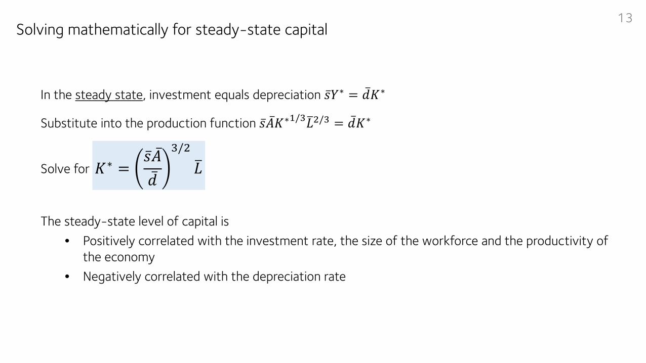
In the steady state, investment equals depreciation �̅�𝑠𝑌𝑌∗ = �̅�𝑑𝐾𝐾∗

Substitute into the production function �̅�𝑠�̅�𝐴𝐾𝐾∗1/3�𝐿𝐿2/3 = �̅�𝑑𝐾𝐾∗

Solve for

The steady-state level of capital is

• Positively correlated with the investment rate, the size of the workforce and the productivity of the economy

• Negatively correlated with the depreciation rate

Solving mathematically for steady-state capital13

𝐾𝐾∗ =�̅�𝑠�̅�𝐴�̅�𝑑

3/2�𝐿𝐿

Plug 𝐾𝐾∗ into the production function to get

• Higher steady-state production caused by higher productivity and investment rate

• Lower steady-state production caused by faster depreciation

Divide both sides by labour to get output per person (y) in steady state

Note the exponent on productivity is different here (3/2) than in the production model (1)

• Higher productivity has additional effects in the Solow model by leading the economy to accumulate more capital

Solving mathematically for steady-state output14

𝑌𝑌∗ =�̅�𝑠�̅�𝑑

1/2�̅�𝐴3/2�𝐿𝐿

𝑦𝑦∗ ≡𝑌𝑌∗

𝐿𝐿∗=

�̅�𝑠�̅�𝑑

1/2�̅�𝐴3/2

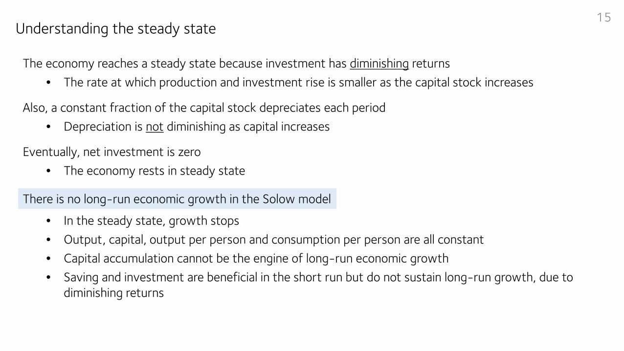
Understanding the steady state15

The economy reaches a steady state because investment has diminishing returns

• The rate at which production and investment rise is smaller as the capital stock increases

Also, a constant fraction of the capital stock depreciates each period

• Depreciation is not diminishing as capital increases

Eventually, net investment is zero

• The economy rests in steady state

• In the steady state, growth stops

• Output, capital, output per person and consumption per person are all constant

• Capital accumulation cannot be the engine of long-run economic growth

• Saving and investment are beneficial in the short run but do not sustain long-run growth, due to diminishing returns

There is no long-run economic growth in the Solow model

Experiments in the Solow model - an increase in �̅�𝑠16

Suppose the investment rate increases permanently for exogenous reasons

• The investment curve �̅�𝑠𝑌𝑌 → �̅�𝑠′𝑌𝑌rotates upwards

• The depreciations curve �̅�𝑑𝐾𝐾 remains unchanged

• The capital stock increases by transition dynamics to reach the new steady state because investment exceeds depreciation

• The new steady state �̅�𝑠′𝑌𝑌 =�̅�𝑑𝐾𝐾 is located to the right

�̅�𝑠 → �̅�𝑠′

17What happens to output in response to the increase in the investment rate?

The rise in investment leads capital to accumulate over time

This higher capital causes output to rise as well

Output increases from its initial steady-state level 𝑌𝑌∗ to the new steady state 𝑌𝑌∗∗

Experiments in the Solow model - an increase in �̅�𝑑18

Suppose the depreciation rate is exogenously shocked to a higher rate

• The depreciations curve �̅�𝑑𝐾𝐾 rotates upwards

• The investment curve �̅�𝑠𝑌𝑌 → �̅�𝑠′𝑌𝑌remains unchanged

• The capital stock declines by transition dynamics to reach the new steady state because depreciation exceeds investment

• The new steady state �̅�𝑠′𝑌𝑌 =�̅�𝑑𝐾𝐾 is located to the left

�̅�𝑑 → �̅�𝑑′

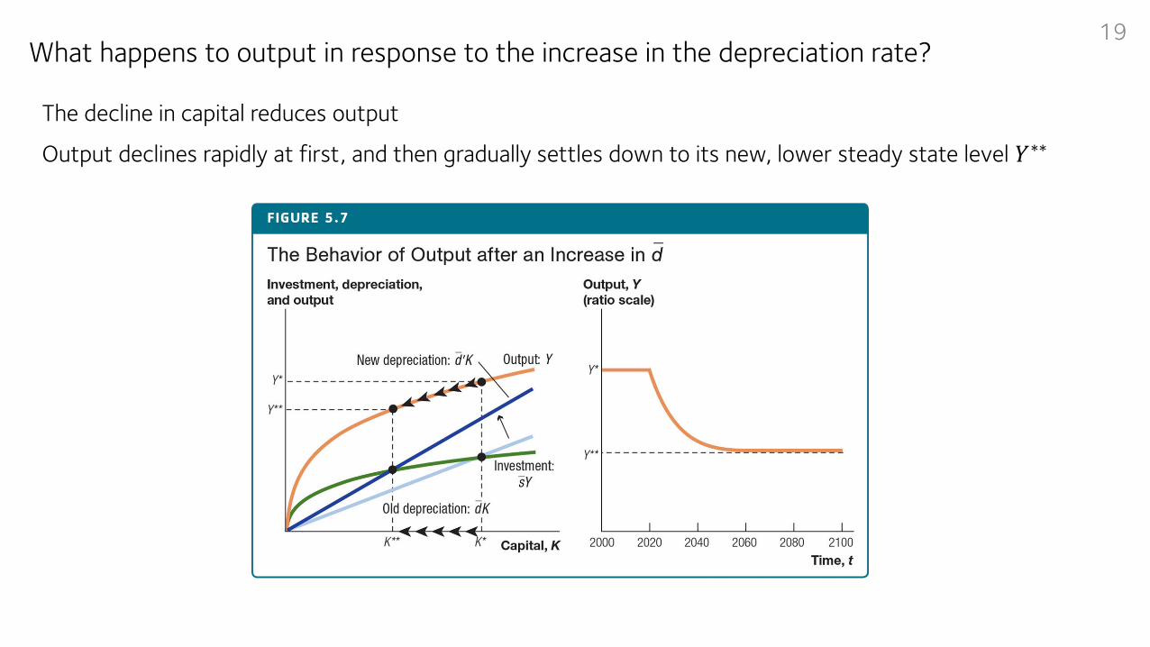
19What happens to output in response to the increase in the depreciation rate?

The decline in capital reduces output

Output declines rapidly at first, and then gradually settles down to its new, lower steady state level 𝑌𝑌∗∗

Next lecture20

Look at data through the lens of the Solow growth model

Ideas as a source of economic growth