The solution of high dimensional elliptic PDEs with random...

The solution of high dimensional elliptic PDEswith random data

Ivan Graham, University of Bath, UK.

Joint work with:

Frances Kuo, Ian Sloan (New South Wales)Dirk Nuyens (Leuven)Rob Scheichl (Bath)

CUHK April 2016

High dimensional Problems: PDE with random data

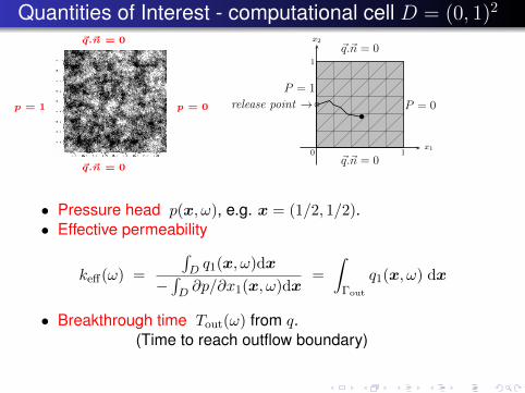
• Many problems involve PDEs with spatially varying datawhich is subject to uncertainty.

Example: groundwater flow in rock underground.

• Uncertainty enters the PDE through its coefficients. (randomfields). The quantity of interest: is a random number or fieldderived from the PDE solution.

Examples: (i) pressure in medium, (ii) effective permeability,(iii) breakthrough time of a pollution plume .

• Typical Computational Goal: expected value of quantity ofinterest.

This is the Forward problem of uncertainty quantification

Some ingredients

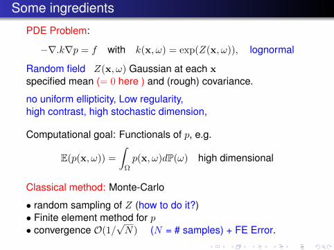
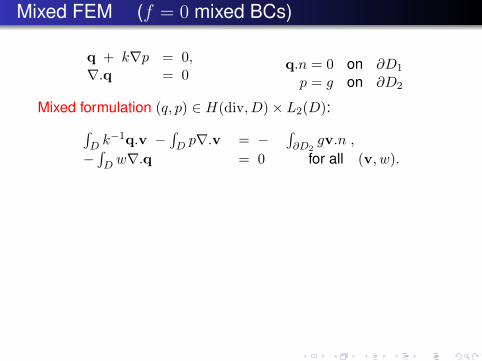
PDE Problem:

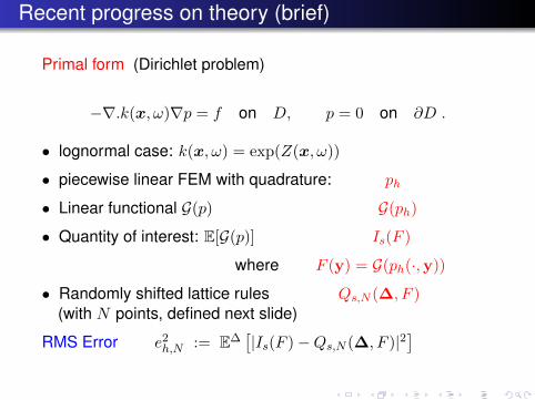
−∇.k∇p = f with k(x, ω) = exp(Z(x, ω)), lognormal

Random field Z(x, ω) Gaussian at each xspecified mean (= 0 here ) and (rough) covariance.

no uniform ellipticity, Low regularity,high contrast, high stochastic dimension,

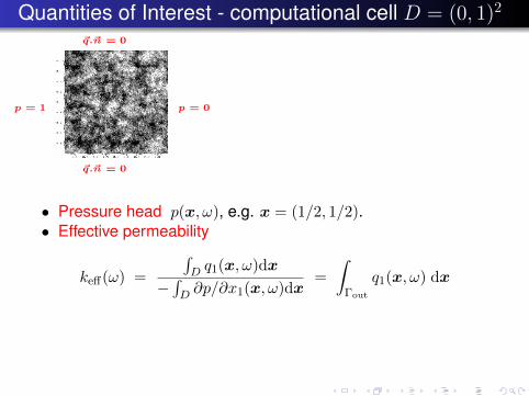
Computational goal: Functionals of p, e.g.

E(p(x, ω)) =

∫Ωp(x, ω)dP(ω) high dimensional

Classical method: Monte-Carlo

• random sampling of Z (how to do it?)• Finite element method for p• convergence O(1/

√N) (N = # samples) + FE Error.

Outline of talk

Part I: Algorithm: circulant embedding with Quasi-Monte Carlo

IGG, Kuo, Nuyens, Scheichl, Sloan JCP 2011

Part II: Rigorous error estimates

IGG, Kuo, Nicholls, Scheichl, Schwab, SloanNumer Math 2014

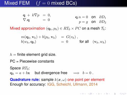
IGG, Scheichl, UllmannStochastic PDE: Analysis and Computation 2014

IGG, Kuo, Nuyens, Scheichl, Sloan in preparation 2016

Gaussian Random Fields (more generally)

PDE Problem:

−∇.k∇p = f + Boundary conditions k = exp(Z)

Covariance function: (centred) stationary field:

E[Z(x, ·)Z(y, ·)] = ρ(x− y), ρ positive definite

Examples:ρ(x− y) = σ2 exp

(− ‖x− y‖/λ

)“exponential”.

ρ(x− y) = σ2 exp(− ‖x− y‖2/λ

)“Gaussian”.

σ2 = variance , λ = lengthscale

The Matern family: ρ = ρβ, β ∈ [1/2,∞).Limiting cases: exponential (β = 1/2), Gaussian (β =∞).

Gaussian Random Fields (more generally)

Loss of uniform ellipticity and boundedness: for all ε > 0:

min[P(k(x, ·) < ε), P(k(x, ·)) > ε−1)] > 0

Mild smoothness condition on ρ(0):Karhunen-Loeve (KL) Expansion: (a.s. convergence)

Z(x, ω) =

∞∑j=1

√µjξj(x)Yj(ω) Yj ∼ N(0, 1)

(ξj , µj) eigenpairs of covariance operator with kernel ρ(x− y).

Kolmogorov’s theorem: With probability 1,k(x, ω) ∈ Ct(D), with t ∈ [0, β)

In fact, for all q ∈ (1,∞),• k ∈ Lq(Ω, Ct(D)),• and ‖p‖Lq(Ω,H1

0 (D)) ≤ ‖a−1min‖Lq(Ω)‖f‖H−1 (Dirichlet problem).

Non-smooth fields : a typical realization (exponential)

λ - “frequency”: Finite element accuracy requires h ≈ λ/10

σ2 - “amplitude”:

maxx k(x, ω)

minx k(x, ω)∼ exp(σ) high contrast

Mixed FEM (f = 0 mixed BCs)

q + k∇p = 0,∇.q = 0

q.n = 0 on ∂D1

p = g on ∂D2

Mixed formulation (q, p) ∈ H(div, D)× L2(D):∫D k−1q.v −

∫D p∇.v = −

∫∂D2

gv.n ,

−∫D w∇.q = 0 for all (v, w).

h = finite element grid size.

PC = Piecewise constants

Space RT0:qh = a + bx but divergence free =⇒ b = 0 .

Quadrature rule: sample k(x, ω) one point per elementEnough for accuracy:IGG, Scheichl, Ullmann,2015


q + k∇p = 0,∇.q = 0

q.n = 0 on ∂D1

p = g on ∂D2

Mixed formulation (q, p) ∈ H(div, D)× L2(D):

m(q,v) + b(p,v) = G(v) ,b(w,q) = 0 for all (v, w).






q + k∇p = 0,∇.q = 0

q.n = 0 on ∂D1

p = g on ∂D2

Mixed approximation (qh, ph) ∈ RT0 × PC on a mesh Th:

m(qh,vh) + b(ph,vh) = G(vh) ,b(wh,qh) = 0 for all (vh, wh)






q + k∇p = 0,∇.q = 0

q.n = 0 on ∂D1

p = g on ∂D2





Space RT0:qh = a+ bx but divergence free =⇒ b = 0 .


q + k∇p = 0,∇.q = 0

q.n = 0 on ∂D1

p = g on ∂D2





Space RT0:qh = a+ bx but divergence free =⇒ b = 0 .

Quadrature rule: sample k(x, ω) one point per elementEnough for accuracy: IGG, Scheichl, Ullmann, 2014

Quantities of Interest - computational cell D = (0, 1)2

p = 1 p = 0

~q.~n = 0

~q.~n = 0

1

• Pressure head p(x, ω), e.g. x = (1/2, 1/2).• Effective permeability

keff(ω) =

∫D q1(x, ω)dx

−∫D ∂p/∂x1(x, ω)dx

=

∫Γout

q1(x, ω) dx


p = 1 p = 0

~q.~n = 0

~q.~n = 0

1

0

1

1x1

x2

P = 1

P = 0

~q.~n = 0

~q.~n = 0

release point →•

1


keff(ω) =

∫D q1(x, ω)dx

−∫D ∂p/∂x1(x, ω)dx

=

∫Γout

q1(x, ω) dx

• Breakthrough time Tout(ω) from q.(Time to reach outflow boundary)


p = 1 p = 0

~q.~n = 0

~q.~n = 0

1

0

1

1x1

x2

P = 1

P = 0

~q.~n = 0

~q.~n = 0

release point →•

1


keff(ω) =

∫D q1(x, ω)dx

−∫D ∂p/∂x1(x, ω)dx

=

∫Γout

q1(x, ω) dx

• Breakthrough time Tout(ω) from q.(Time to reach outflow boundary)

• General format: find E[G(p,q)] - some functional G(p,q).

Sampling by K-L truncation : the effect of lengthscale

Z(x, ω) =

∞∑j=1

√µjξj(x)Yj(ω)

exponential covariance in 1D

log log plot of µj for 1 ≤ j ≤ 500:

100 101 102 103

10−6

10−5

10−4

10−3

10−2

10−1

100

Plateau before decay starts

λ = 1λ = 0.1λ = 0.01

An extreme eigenvalue solverchallenge!

Avoiding KL truncation: discretize first in space

Approximation of E[G(p)] by E[G(ph)] (focus on pressure)

FEM + quadrature requires random vectorZ := Z(xi) at M quadrature points

Covariance Matrix: Ri,j = ρ(xi − xj) M ×M

Seek matrix decomposition:

R = BB> (*)

where B is M × s, s ≥M .

Then (finite “discrete KL” expansion)

Z(ω) = BY (ω), where Y ∼ N(0, 1)s i.i.d.

BecauseE[ZZ>] = E[BYY>B>] = BB> = R

M ∼ h−d and so s very large so (*) expensive(?), but....

Sampling via Circulant Embedding

For

not restrictive︷︸︸︷uniform grids and stationary fields: R is block Toeplitz

Embed R into C - block circulant s× s (Typically s ∼ (2d)M )

0 0.5 1 1.5 2 2.5 30.2

0.3

0.4

0.5

0.6

0.7

0.8

0.9

1

C =

[R AAT B

]

(Cheap) Factorization: C = FΛFH (by FFT)implies Real Factorization: C = BBT (provided diag(Λ) ≥ 0)

E[G(p)] ≈∫RsF (y)

s∏j=1

φ(yj)dy, F (y) = G(ph(·,y))

=

∫[0,1]s

F (Φ−1s (v))dv =: Is(F ) .

φ(y) = exp(−y2/2)/√

2π, Φ−1s = inv. cum. normal

FEM (h) + high dimensional integration (?)

Integration over [0, 1]s (very large s): QMC methods

∫[0,1]s

f(z) dz ≈ 1

N

N∑k=1

f(z(k))

Monte Carlo methodz(k) random uniformO(N−1/2) convergenceorder of variables irrelevant

Quasi-Monte Carlo methodz(k) deterministicclose to O(N−1) convergenceorder of variables very important

64 random points

••

•

••

•

•

•

•

•

•

•••

•

•• •

•

•

•

•

•

•

•

•

•

•

•

•

•

•

•••

•

•

••

•

•

••

• ••

••

•

••

••

••

•

•

•

•

•

•

••

•

64 Sobol′ points•

•

•

•

•

•

•

••

•

•

•

•

•

•

•

•

•

•

•

•

•

•

••

•

•

•

•

•

•

•

•

•

•

•

•

•

•

••

•

•

•

•

•

•

•

•

•

•

•

•

•

•

••

•

•

•

•

•

•

•

64 lattice points•

•

•

•

•

•

•

•

•

•

•

•

•

•

•

•

•

•

•

•

•

•

•

•

•

•

•

•

•

•

•

•

•

•

•

•

•

•

•

•

•

•

•

•

•

•

•

•

•

•

•

•

•

•

•

•

•

•

•

•

•

•

•

•

1

Numerical Results

Covariance

r(x,y) = σ2 exp(− ‖x− y‖1/λ

).

( ‖ · ‖2 similar).

Case 1 Case 2 Case 3 Case 4 Case 5

σ2 = 1 σ2 = 1 σ2 = 1 σ2 = 3 σ2 = 3λ = 1 λ = 0.3 λ = 0.1 λ = 1 λ = 0.1

FEM: Uniform grid h = 1/m on (0, 1)2, M ∼ m2.

Sampling: circulant embedding via FFT (dimension s ≥ 4M )

High dimensional integration: QMC with N Sobol’ points

Algorithm profile

Time (sec) for N = 1000, CASE 1:

percentages in red, orders in blue

m s Setup InvN FFT AMG TOT33 4.1 (+3) 0.00 1.0 17 0.22 4 4.5 76 5.965 1.7 (+4) 0.01 3.9 17 1.2 5 16.5 75 22

129 6.6 (+4) 0.06 15 16 5.1 6 67 73 92257 2.6 (+5) 0.15 62 16 31 8 290 73 400513 1.0 (+6) 0.6 258 15 145 8 1280 73 1750

m2 m2 m2 m2 logm ∼ m2 ∼ m2

InvN = Inversion of cumulative normal

AMG = Algebraic Multigrid = Fast system solver

Algorithm profile

Time (sec) for N = 1000, CASE 1:

percentages in red, orders in blue

m s Setup InvN FFT AMG TOT33 4.1 (+3) 0.00 1.0 17 0.22 4 4.5 76 5.965 1.7 (+4) 0.01 3.9 17 1.2 5 16.5 75 22

129 6.6 (+4) 0.06 15 16 5.1 6 67 73 92257 2.6 (+5) 0.15 62 16 31 8 290 73 400513 1.0 (+6) 0.6 258 15 145 8 1280 73 1750

m2 m2 m2 m2 logm ∼ m2 ∼ m2

InvN = Inversion of cumulative normal

AMG = Algebraic Multigrid = Fast system solver

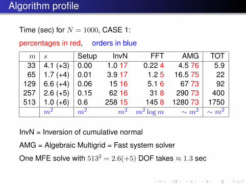
One MFE solve with 5132 = 2.6(+5) DOF takes ≈ 1.3 sec

Standard deviation of mean pressure

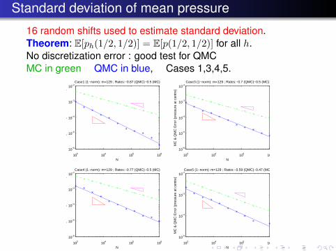
16 random shifts used to estimate standard deviation.Theorem: E[ph(1/2, 1/2)] = E[p(1/2, 1/2)] for all h.No discretization error : good test for QMCMC in green QMC in blue, Cases 1,3,4,5.

103 104 105 106

10−6

10−5

10−4

10−3

10−2

N

MC

& Q

MC

Err

or (

pres

sure

at c

entr

e)

Case1 (1−norm): m=129 ; Rates:−0.87 (QMC)−0.5 (MC)

103 104 105 10

10−6

10−5

10−4

10−3

10−2

N

MC

& Q

MC

Err

or (

pres

sure

at c

entr

e)


103 104 105 106

10−6

10−5

10−4

10−3

10−2

N

MC

& Q

MC

Err

or (

pres

sure

at c

entr

e)


103 104 105 10

10−5

10−4

10−3

10−2

N

MC

& Q

MC

Err

or (

pres

sure

at c

entr

e)Case5 (1−norm): m=129 ; Rates:−0.59 (QMC)−0.47 (MC)

Dimension independence of QMC (and MC)

Standard deviation of mean pressure, Case 4:as m(= 1/h) (and hence s) increasesMC in green QMC in blue

103 104 105 106

10−6

10−5

10−4

10−3

10−2

N

MC

& Q

MC

Err

or (

pres

sure

at c

entr

e)


103 104 105 10

10−6

10−5

10−4

10−3

10−2

N

MC

& Q

MC

Err

or (

pres

sure

at c

entr

e)


103 104 105 106

10−6

10−5

10−4

10−3

10−2

N

MC

& Q

MC

Err

or (

pres

sure

at c

entr

e)


103 104 105 10

10−6

10−5

10−4

10−3

10−2

N

MC

& Q

MC

Err

or (

pres

sure

at c

entr

e)


Effective permeability keff

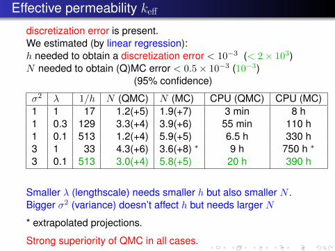
discretization error is present.We estimated (by linear regression):h needed to obtain a discretization error < 10−3 (< 2× 103)N needed to obtain (Q)MC error < 0.5× 10−3 (10−3)

(95% confidence)

σ2 λ 1/h N (QMC) N (MC) CPU (QMC) CPU (MC)1 1 17 1.2(+5) 1.9(+7) 3 min 8 h1 0.3 129 3.3(+4) 3.9(+6) 55 min 110 h1 0.1 513 1.2(+4) 5.9(+5) 6.5 h 330 h3 1 33 4.3(+6) 3.6(+8) ∗ 9 h 750 h ∗

3 0.1 513 3.0(+4) 5.8(+5) 20 h 390 h

Smaller λ (lengthscale) needs smaller h but also smaller N .Bigger σ2 (variance) doesn’t affect h but needs larger N

* extrapolated projections.

Strong superiority of QMC in all cases.

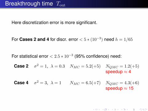
Breakthrough time Tout

Here discretization error is more significant.

For Cases 2 and 4 for discr. error < 5 ∗ (10−3) need h = 1/65

For statistical error < 2.5 ∗ 10−3 (95% confidence) need:

Case 2 σ2 = 1, λ = 0.3 NMC = 5.2(+5) NQMC = 1.2(+5)speedup ≈ 4

Case 4 σ2 = 3, λ = 1 NMC = 6.5(+7) NQMC = 4.3(+6)speedup ≈ 15

Breakthrough time, Cases 1-4

103 104 105 106

10−4

10−3

10−2

10−1

N

MC

& Q

MC

Err

or (

exit

time)


103 104 105 106

10−4

10−3

10−2

10−1

N

MC

& Q

MC

Err

or (

exit

time)


103 104 105 106

10−4

10−3

10−2

10−1

N

MC

& Q

MC

Err

or (

exit

time)


103 104 105 106

10−3

10−2

10−1

100

N

MC

& Q

MC

Err

or (

exit

time)


MC in green QMC in blue

QMC still superior but rate 1/N is now missing.

Recent progress on theory (brief)

Primal form (Dirichlet problem)

−∇.k(x, ω)∇p = f on D, p = 0 on ∂D .

• lognormal case: k(x, ω) = exp(Z(x, ω))

• piecewise linear FEM with quadrature: ph

• Linear functional G(p) G(ph)

• Quantity of interest: E[G(p)] Is(F )

where F (y) = G(ph(·,y))

• Randomly shifted lattice rules Qs,N (∆, F )(with N points, defined next slide)

RMS Error e2h,N := E∆

[|Is(F )−Qs,N (∆, F )|2

]

Some QMC Theory (Lattice rules)

Is(F ) :=

∫RsF (y)

∏φ(yj)dy =

∫[0,1]s

F (Φ−1s (z))dz

Qs,N (∆;F ) :=1

N

N∑i=1

F

(Φ−1s

(frac

(i z

N+ ∆

)))generating vector: z ∈ Ns, 1 ≤ zj ≤ N − 1random shift ∆ ∈ [0, 1]s uniformly distributed.

Weighted Sobolev norm: ‖F‖2s,γ :=∑

u⊆1:s1γuJu(F )2

where Ju(F )2 =∫R|u|

(∫Rs−|u|

∂|u|F

∂yu(yu;y1:s\u)

∏j∈1:s\u

φ(yj) dy1:s\u

)2∏j∈u

ψ2j (yj) dyu

γu - controls relative importance of the derivatives

ψj(yj) = exp(−αj |yj |) - controls behaviour as |y| → ∞

QMC Theory...

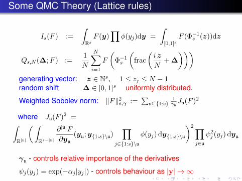
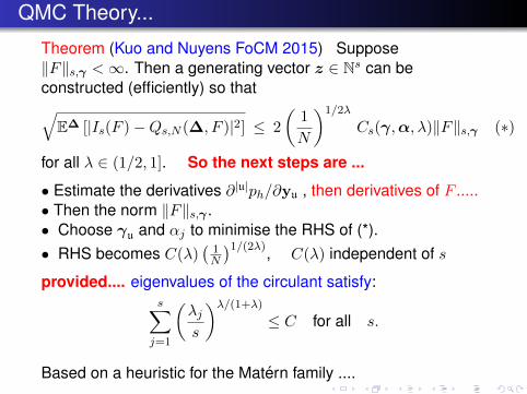
Theorem (Kuo and Nuyens FoCM 2015) Suppose‖F‖s,γ <∞. Then a generating vector z ∈ Ns can beconstructed (efficiently) so that√

E∆ [|Is(F )−Qs,N (∆, F )|2] ≤ 2

(1

N

)1/2λ

Cs(γ,α, λ)‖F‖s,γ (∗)

for all λ ∈ (1/2, 1]. So the next steps are ...

• Estimate the derivatives ∂|u|ph/∂yu , then derivatives of F .....• Then the norm ‖F‖s,γ .• Choose γu and αj to minimise the RHS of (*).• RHS becomes C(λ)

(1N

)1/(2λ), C(λ) independent of s

provided.... eigenvalues of the circulant satisfy:s∑j=1

(λjs

)λ/(1+λ)

≤ C for all s.

Based on a heuristic for the Matern family ....

Rates for the Matern class

• Dimension independent rate O(

1N−(1−δ)

)δ arbitrarily small, if

ν > 2.

• Dimension independent rate at least O(

1N

)1/2 if ν > 1

Heuristic assumes eigenvalues of the circulant approacheigenvalues of the corresponding periodic covariance integraloperator.

Conclusion:

For Matern parameter ν large enough, combined FE and QMCerror:√

E∆ [|E[G(p)]−Qs,N (∆,G(ph))|2] ≤ C[h2 +N−(1−δ)].

with δ arbitrarily close to 0 independent of dimension s.

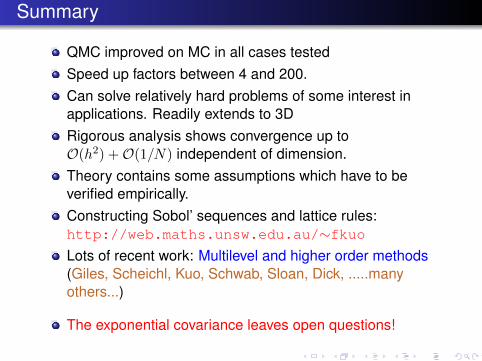
Summary

QMC improved on MC in all cases testedSpeed up factors between 4 and 200.Can solve relatively hard problems of some interest inapplications. Readily extends to 3DRigorous analysis shows convergence up toO(h2) +O(1/N) independent of dimension.Theory contains some assumptions which have to beverified empirically.Constructing Sobol’ sequences and lattice rules:http://web.maths.unsw.edu.au/∼fkuoLots of recent work: Multilevel and higher order methods(Giles, Scheichl, Kuo, Schwab, Sloan, Dick, .....manyothers...)

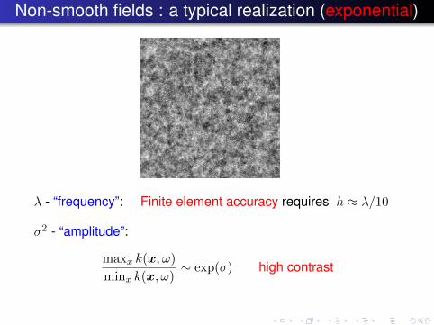
The exponential covariance leaves open questions!

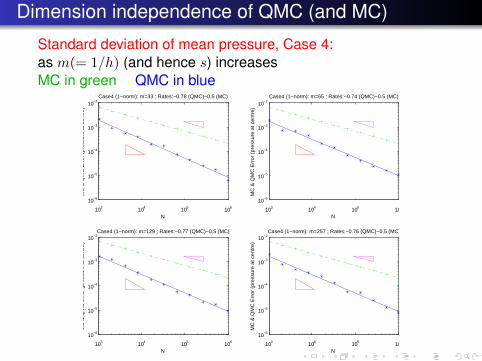
Dimension independence of QMC (and MC)

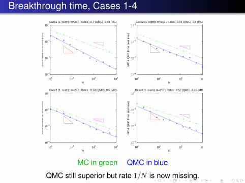
Standard deviation of mean pressure, Case 4:as m(= 1/h) (and hence s) increasesMC in green QMC in blue

103 104 105 106

10−6

10−5

10−4

10−3

10−2

N

MC

& Q

MC

Err

or (

pres

sure

at c

entr

e)


103 104 105 10

10−6

10−5

10−4

10−3

10−2

N

MC

& Q

MC

Err

or (

pres

sure

at c

entr

e)


103 104 105 106

10−6

10−5

10−4

10−3

10−2

N

MC

& Q

MC

Err

or (

pres

sure

at c

entr

e)


103 104 105 10

10−6

10−5

10−4

10−3

10−2

N

MC

& Q

MC

Err

or (

pres

sure

at c

entr

e)


Date post:	08-Jun-2018
Category:	Documents
Upload:	dokhanh
View:	217 times
Download:	0 times

The solution of high dimensional elliptic PDEs with random...

Documents