The spatial scale of habitat selection by red deer

James A. Schaefer, Nicolas Morellet, Dominique Pepin, and Helene Verheyden

Abstract: Accounting for spatial scale is essential for understanding habitat selection, but few studies have used spa-tial statistics to reveal the characteristic scale at which organisms respond to their environment. We studied habitatselection by GPS-tracked red deer (Cervus elaphus L., 1758) in the Pyrenees Mountains, France, by applying a geo-statistical model that compares autocorrelation of a resource between used and available sites to uncover the scaleat which animals assess habitat. Using an artificial landscape, we demonstrated that the model can handle discretehabitat classes. Based on conventional hierarchical analysis, deer selected for open habitat, especially meadow, andavoided coniferous forest, more strongly at the coarse level of the home range than GPS locations. Home ranges ex-hibited generally lower autocorrelation in elevation and meadow habitat than random locations within the populationrange, indicative of preference for high habitat heterogeneity. Mean maximum discrepancy in autocorrelation, whichwas more pronounced at the level of the home range than GPS locations, occurred at 830 m for meadow habitatand at 1511 m for elevation, suggesting that red deer responded to their environment at this scale. Our study dem-onstrates how spatial statistics can serve as an instructive complement to conventional approaches to habitat selec-tion.

Resume : L’etude de l’echelle spatiale est essentielle pour comprendre la selection de l’habitat, mais peu d’etudesont utilise des statistiques spatiales pour reveler l’echelle caracteristique a laquelle un organisme repond a son envi-ronnement. Nous avons etudie la selection de l’habitat par des cerfs rouges (Cervus elaphus L., 1758) suivis parGPS dans les montagnes pyreneennes, en France, en appliquant un modele geostatistique, qui compare l’autocorre-lation d’une ressource entre les sites utilises et disponibles pour decouvrir l’echelle a laquelle les animaux evaluentleur habitat. A partir d’un paysage artificiel, nous demontrons que ce modele peut etre generalise pour traiter desclasses discretes d’habitat. D’apres une analyse hierarchique conventionnelle, les cerfs selectionnent un habitat ouvert,plus particulierement les prairies, et evitent les forets de coniferes, de facon plus marquee au niveau plus grossierdu domaine vital que celui des localisations GPS. Les domaines revelent generalement une plus faible autocorrela-tion pour l’altitude et l’habitat prairie que les localisations aleatoires dans le domaine populationnel, revelateur d’unepreference pour une forte heterogeneite d’habitats. L’ecart moyen maximum d’autocorrelation, plus prononce al’echelle du domaine individuel que des localisations GPS, est de 830 m pour l’habitat prairie et de 1511 m pourl’altitude, ce qui laisse croire que le cerf reagit a son environnement a cette echelle. Notre etude demontre commentles statistiques spatiales peuvent servir de complement instructif aux approches conventionnelles de selection del’habitat.

Introduction

Spatial scale has become a prominent feature in the studyof habitat selection (Johnson 1980; Senft et al. 1987; Boyce2006). Because inferences about habitat selection are oftensensitive to scale, investigations now commonly span sev-eral levels of analysis, between the grain of the individualanimal location and the extent of a species range. The bene-fits of a multiscale framework are many — for example, byhelping to overcome arbitrary notions of availability(Schaefer and Messier 1995), facilitating comparisons acrossspecies (Ihl and Klein 2001; Jenkins et al. 2007), and poten-tially revealing the most significant population limiting fac-tors (Rettie and Messier 2000).

While a hierarchical approach is informative, determiningthe explicit scales at which animals select resources, in unitsof area or distance, is still desirable. The ‘‘characteristic

scale’’ at which organisms react to their environment is es-sential for understanding patterns of species occupancy andresponses to landscape change (Olden et al. 2004), and suchscales may not be intuitive. Mule deer (Odocoileus hemio-nus (Rafinesque, 1817)), for instance, appear to assess theirsurroundings well beyond the home range when establishinga home range (Bowyer and Kie 2006).

Spatial statistics are the basis of a recent geostatisticalmodel to detect these scales (Mayor et al. 2007; Schaeferand Mayor 2007). The premise of the model is that habitatselection may be regarded as a shift, often a reduction, inthe variance of resources or conditions. By comparing thespatial structure of a resource at sites used by an organismand the general environment, the scale of perception is re-vealed — the point of maximum divergence in either semi-variance or spatial autocorrelation. In studies of habitatselection, geostatistics have been applied to describe the

Received 14 April 2008. Accepted 3 October 2008. Published on the NRC Research Press Web site at cjz.nrc.ca on 18 November 2008.

J.A. Schaefer.1 Biology Department, Trent University, 1600 West Bank Drive, Peterborough, ON K9J 7B8, Canada.N. Morellet, D. Pepin, and H. Verheyden. Institut National de la Recherche Agronomique – Comportement et Ecologie de la FauneSauvage, chemin de Borde Rouge-Auzeville, B.P. 52627, F 31326 Castanet-Tolosan CEDEX, France.

1Corresponding author (e-mail: jschaefer@trentu.ca).

1337

Can. J. Zool. 86: 1337–1345 (2008) doi:10.1139/Z08-122 # 2008 NRC Canada

distribution of resources within a study area (e.g., Meiseland Turner 1998; Boyce et al. 2003) but not to examine‘‘used’’ vs. ‘‘available’’ sites. This is the key comparisonthat may reveal the extent of organism response to the envi-ronment (Schaefer and Mayor 2007).

The geostatistical model is appropriate when a resource istreated as a continuous variable. Although spatial statisticshave been used to reveal the patterns of binary landscapes(Carpenter and Chaney 1983; Dale and Blundon 1990), it isunclear whether the model can accommodate discrete habitatclasses, a common circumstance when habitats are mappedby remote-sensing (Table 1).

Here, we explored the application of this geostatisticalmodel of habitat selection to GPS-tracked red deer (Cervuselaphus L., 1758) in the Pyrenees Mountains in southwest-ern France (Fig. 1). First, we tested the model using an arti-ficial landscape categorized into discrete habitat types. Weshow that the model is capable of uncovering scales ofselection when habitats are viewed under a binary classifica-tion. Second, we used the model to study habitat selectionby red deer. From GPS tracking of 11 individuals, we ana-

lysed the patterns of habitat selection based on a conven-tional approach of use vs. availability (Thomas and Taylor1990) at three hierarchical levels: population range, homeranges, and GPS locations. Then, using two habitat features(meadow and elevation), we used the geostatistical model touncover the explicit scales at which these animals assesstheir montane environment.

Materials and methods

Test of the model with discrete habitatsWe followed the general approach of Schaefer and Mayor

(2007) to explore the suitability of the geostatistical modelusing strict binary habitat classes. First, we built a toroidallandscape of 500 sites with variable levels of a resource us-ing the logistic equation with a stochastic variable (x) to setthe resource abundance (y) at each site:

½1� yiþ1 ¼ yier½1�ðyi=KÞ�þx

where yi+1 is the resource level in the adjacent cell, yi is theresource level in the ith site, e is base of the natural loga-

Table 1. Habitat classes and characteristics in the study area in the Pyrenees Mountains, France.

Habitat type Code Floristic attributesMeadow MEAD Grasses and forbsBirch margin BIRCH Betula pubescens, myrtle blueberries (Vaccinium myrtillus L.), grassesJuniper grassland JUNIP Grasses, Juniperus communis, Calluna vulgaris, Vaccinium spp.Oak forest OAK Quercus sp.Other moorland OTHER Pteridium aquilinum, Rhododendron ferrugineumDeciduous forest DECID Quercus sp., common hazel (Corylus avellana L.), sweet chestnut (Castanea sativa Mill.),

Fagus sylvaticaHeather moorland HEATH Calluna spp., grasses, Vaccinium spp.Mountain pasture PAST Grasses and forbs, Calluna spp., Vaccinium spp.Coniferous forest CONIF Abies alba, Fagus sylvatica

Fig. 1. Population range (broken line) and home ranges (solid lines) for red deer (Cervus elaphus) in the Pyrenees Mountains (arrow in theinset map), France.

1338 Can. J. Zool. Vol. 86, 2008

# 2008 NRC Canada

rithm, r is the exponential rate of change, K is the stableequilibrium point, and x is a normally distributed randomvariate with a mean of 0 and a standard deviation of 0.2.We set r to 0.1 and both y1 and K to 100.

We then populated this landscape with animals that se-lected sites based on the surrounding neighbourhood, i.e.,the distance from that site to the most distant site ofperception. The neighbourhood extended in both direc-

tions. A site was used if its resource abundance exceededthe neighbourhood mean. We ran the model with neigh-bourhoods of 5, 10, and 20 units. For each neighbourhood,the model was run 100 times on the same series of land-scapes.

To fit this continuous landscape into a binary classifica-tion, we categorized the value at each site to either 0 or 1based on whether its resource level was above or below the

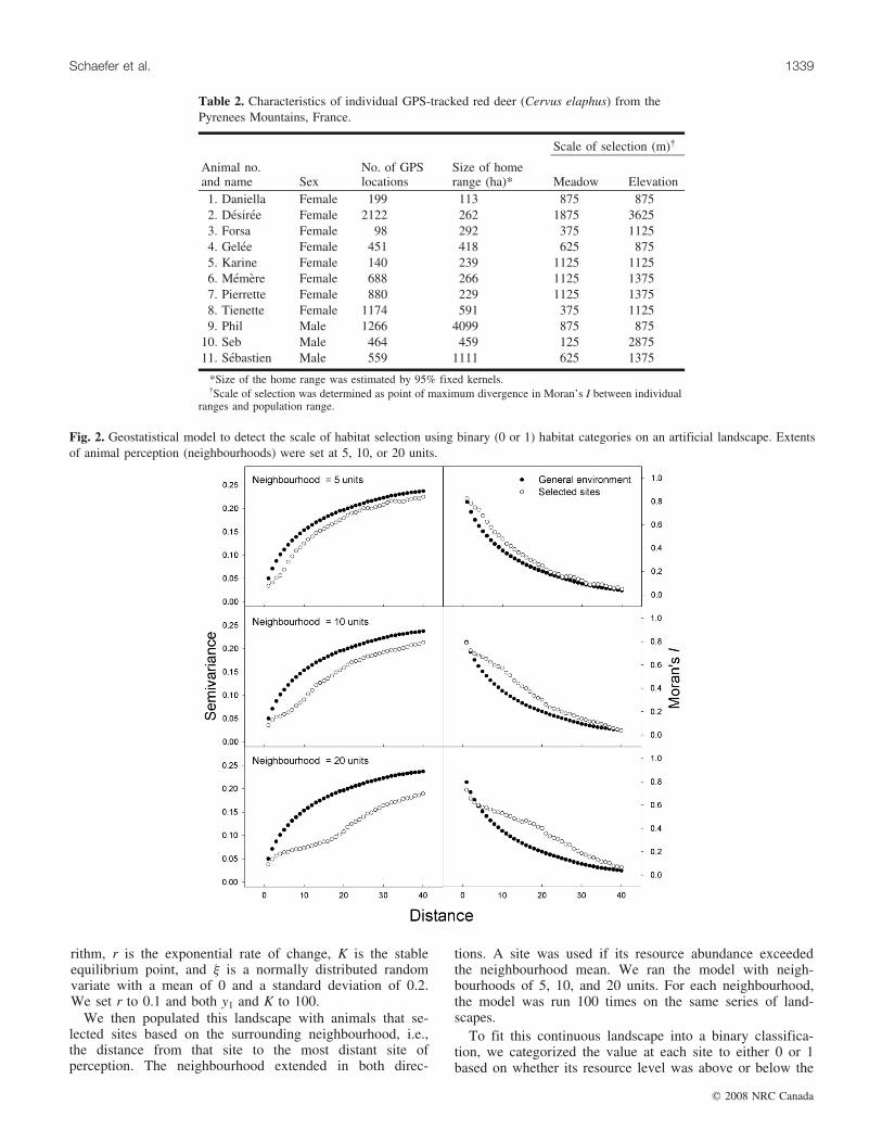
Table 2. Characteristics of individual GPS-tracked red deer (Cervus elaphus) from thePyrenees Mountains, France.

Scale of selection (m){

Animal no.and name Sex

No. of GPSlocations

Size of homerange (ha)* Meadow Elevation

1. Daniella Female 199 113 875 8752. Desiree Female 2122 262 1875 36253. Forsa Female 98 292 375 11254. Gelee Female 451 418 625 8755. Karine Female 140 239 1125 11256. Memere Female 688 266 1125 13757. Pierrette Female 880 229 1125 13758. Tienette Female 1174 591 375 11259. Phil Male 1266 4099 875 875

10. Seb Male 464 459 125 287511. Sebastien Male 559 1111 625 1375

*Size of the home range was estimated by 95% fixed kernels.{Scale of selection was determined as point of maximum divergence in Moran’s I between individual

ranges and population range.

Fig. 2. Geostatistical model to detect the scale of habitat selection using binary (0 or 1) habitat categories on an artificial landscape. Extentsof animal perception (neighbourhoods) were set at 5, 10, or 20 units.

Schaefer et al. 1339

# 2008 NRC Canada

mean across the entire landscape, i.e., yi = 0 (if yi > y) oryi = 1 (if yi < y). We also explored the effect of misclassifi-cation of the landscape by altering the classification crite-rion to four other values (y + 1 SD, y + 0.5 SD, y – 0.5SD, and y – 1 SD). The neighbourhood was set at 10 units.

We constructed variograms (semivariance vs. lag dis-tance) and correlograms (Moran’s I vs. lag distance) be-tween all possible pairs of sites, separately for the generalenvironment (all sites) and used sites. The semivariance (g)at some distance (h) is half the sum of the squared differ-ence between pairs (Meisel and Turner 1998):

½2� byðhÞ ¼ 1

2nðhÞXn

i¼1

ðyi � yiþhÞ2

where y is the value of the variable at the ith and (i + h)thsites and n(h) is the number of pairs of sampling locationsseparated by distance h. The value is divided by 2 becausethe summation from 1 to n sampling locations considerseach pair twice in the calculation.

Moran’s I was computed for each distance class, d(Legendre and Legendre 1998):

½3� IðdÞ ¼1W

Pnh¼1

Pni¼1

whiðyh � yÞðyi � yÞ

1n

Pni¼1

ðyi � yÞ2

where whi is 1 when sites h and i are at the distance d andwhi is 0 otherwise. W is the sum of whi for each distanceclass. Moran’s I usually varies between +1 and –1; positivevalues denote positive autocorrelation and negative valuesrepresent negative autocorrelation.

Habitat selection by red deerThe field data were derived from a 180 km2 study area in

the Pyrenees Mountains, southwestern France. Elevationranged between 800 and 2200 m above sea level. Vegetationconsisted mostly of meadows in the bottom of the valleyand, as elevation increased, grassland with common juniper

Fig. 3. Geostatistical model to detect the scale of habitat selection using binary (0 or 1) habitat categories on an artificial landscape.Misclassification of habitat was varied from the mean plus 1 standard deviation (SD) to the mean minus 1 SD. Extent of animal perceptionwas set at 10 units.

1340 Can. J. Zool. Vol. 86, 2008

# 2008 NRC Canada

(Juniperus communis L.) or bracken fern (Pteridium aquili-num (L.) Kuhn), heather moorland (Calluna vulgaris (L.)Hull), and mountain pasture at the top. Coniferous (silverfir, Abies alba Miller) or mixed coniferous forest (withEuropean beech, Fagus sylvatica L.) occurred on hillyslopes especially in north and west faces with margin ofbirch (Betula pubescens Ehrh.) and, in the upper elevations,patches of alpine rose (Rhododendron ferrugineum L.).Deciduous forest dominated by oaks (genus Quercus L.) oc-curred on east and south slopes at low elevation.

Habitats were delineated from SPOT satellite imagery,October 2001, in 20 m � 20 m pixels. The area was sub-jected to a supervised maximum likelihood classificationrecognizing nine vegetation categories (Table 1). To definethese classes, we used existing information supplementedwith field observations. These data included forest mapsfrom the Inventaire Forestier National and from the OfficeNational des Forets, data on habitats grazed by livestock

from the Service d’Utilite Agricole Inter-chambres d’Agri-culture Pyrenees, and a bear habitat map from the OfficeNational de la Chasse et de la Faune Sauvage. We refinedsome broad habitat classes based on vegetation compositionand physionomy. From field surveys, we constructed a‘‘training map’’ of homogeneous habitat patches (forest onsunlight, forest on shadow, open on sunlight, open onshadow) of a trichromic SPOT image covering the studyarea. The four classifications were done to disentangle simi-lar trichromic responses to some forest and green meadowpatches and to shadow. The habitat map was validated usingextended patches of the training map and up to 1000 recordsof vegetation biomass and cover from the field.

Eleven adult deer (8 females, 3 males) were fitted withGPS radio collars (Table 2), programmed to record locationsevery 3 h, with a precision of <30 m. These animals weretreated under authorization certificate no. 31-265, in accord-ance with guidelines from the Canadian Council on AnimalCare. Data were collected from November 2002 to April2004. Elevation was determined from topographic maps.Owing to transmitter malfunctions and mortality of four ani-mals in February and March 2003, there was substantialindividual variation in the duration of tracking (2–12 months)and the number of GPS locations (100 to >2100). Oursample size did not afford the opportunity to investigatevariations owing to sex, time of day, or season, which canbe appreciable for this species (Boyce et al. 2003;McCorquodale 2003).

We conducted analysis of habitat selection at two levels.Home ranges (minimum convex polygon (MCP) aroundeach animal’s GPS locations) were compared with the popu-lation range (MCP surrounding all GPS locations from allindividuals together; Fig. 1); GPS locations were comparedwith home ranges. For each habitat type (Table 1), we com-puted percent use minus percent available (Thomas and Tay-lor 1990), where availability was denoted as the adjacent,higher level in this hierarchy (Schaefer and Messier 1995).We also tested for selection of forest by combining treedhabitats (birch margin, oak, deciduous, and coniferous for-ests) into one. We assesed significance with one samplet tests under the null hypothesis that the mean of percentuse minus percent available was zero.

We applied the geostatistical model, using correlograms,on two variables (meadow and elevation), both of which areimportant to deer (Albon and Langvatn 1992; Mysterud etal. 2001, 2002). Meadow was treated as a binary variable(i.e., meadow = 1; all other habitats = 0). Plots of Moran’sI vs. distance were computed among all possible pairs ofGPS locations, and compared with 5000 random locationsin each home range, as well as 5000 random points withinthe overall population range. Distance classes were set at250 m intervals, to a maximum of 4000 m, the midpoints ofwhich were used in subsequent analyses. Computations wereconducted in SAM verion 1.1 (Rangel et al. 2006) and STA-TISTICA version 7.0 (StatSoft Inc., Tulsa, Oklahoma,USA).

Results

Test of the model with discrete habitatsIn general, variograms and correlograms were effective in

Fig. 4. Use and availability of nine habitat types by red deer(Cervus elaphus) in the Pyrenees Mountains. Availability wasbased on the adjacent, broader scale (i.e., GPS locations vs. homerange, home ranges vs. population range). Each datum representsone animal. Means significantly different from zero are indicatedby * (P < 0.05) or ** (P < 0.01). Habitat codes from Table 1.

Schaefer et al. 1341

# 2008 NRC Canada

uncovering the scale of selection when the simulated land-scape was viewed in a binary classification. In this artificialenvironment when neighbourhoods were set at 5, 10, and 20units, variograms diverged most strongly at scales of 4, 9,and 16 units, whereas for correlograms it was 4, 10, and 18units, respectively (Fig. 2).

The misclassification of habitat only slightly obscured theoutcome of the model (Fig. 3). The neighbourhood of 10units was faithfully displayed as the maximum discrepancyin variograms and correlograms when the classification cri-terion was close to the resource mean (i.e., ±0.5 SD). Whenthe classification diverged even more strongly from themean, (i.e., ±1 SD), the point of divergence became onlyslightly less accurate (range = 8–12 units), but the ability todiscern the peak difference became somewhat more difficult(Fig. 3).

Habitat selection by red deerDeer selected most strongly at the level of the home range

(Fig. 4); they preferred some open habitats (meadow, birchmargin, and juniper), whereas pasture and especially conif-erous forests were avoided. GPS locations differed littlefrom the composition of the home ranges, with the excep-tion of modest avoidance of deciduous forests (t[10] = 2.27,

P = 0.047; Fig. 4). Similarly, when we combined forestedhabitats into one category, deer showed marginal avoidanceof forests at the home range (t[10] = 2.05, P = 0.067) but notat the level of GPS locations (t[10] = 1.42, P = 0.19).

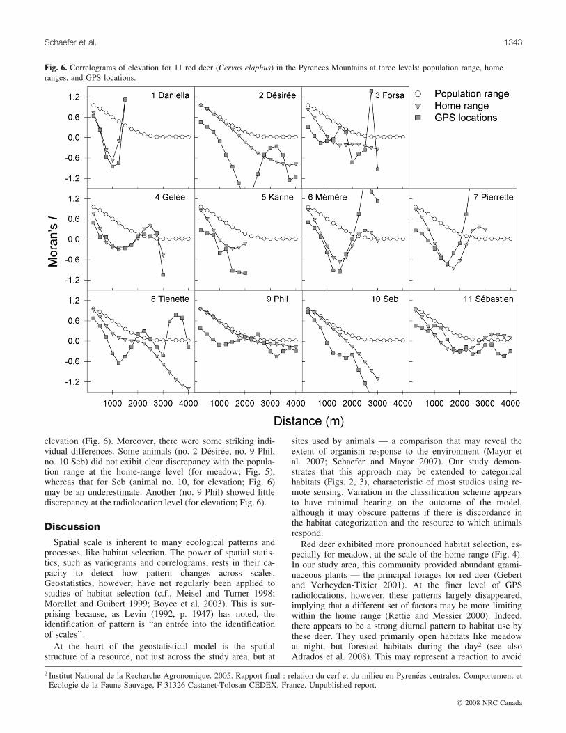
Moran’s I was lower at sites used by deer than in the gen-eral environment (Figs. 5, 6) for both elevation andmeadow, both at the home range and radiolocation level.This indicated greater habitat heterogeneity in sites used byred deer compared with their surroundings. Based on thepoint of maximum discrepancy in Moran’s I between thehome ranges and the population range, deer responded totheir habitat at the scale of several hundred metres: 830 m(±146 SE) for meadow (Fig. 5) and 1511 m (±270 SE) forelevation (Fig. 6; Table 2). The scales of response to theenvironment, determined by the model, were not predictablefrom home-range size quantified using a 95% kernel estima-tor; there was no significant correlation between them(meadow: r = –0.064, P = 0.852; elevation: r = –0.235, P =0.487).

The model was sensitive to the level of comparison.Based on the point of maximum discrepancy in Moran’s Ibetween GPS locations and population range, deer re-sponded at a similar but slightly finer scale: 625 m(±126 SE) for meadow (Fig. 5) and 943 m (±143 SE) for

Fig. 5. Correlograms of meadow habitat for 11 red deer (Cervus elaphus) in the Pyrenees Mountains at three levels: population range, homeranges, and GPS locations.

1342 Can. J. Zool. Vol. 86, 2008

# 2008 NRC Canada

elevation (Fig. 6). Moreover, there were some striking indi-vidual differences. Some animals (no. 2 Desiree, no. 9 Phil,no. 10 Seb) did not exibit clear discrepancy with the popula-tion range at the home-range level (for meadow; Fig. 5),whereas that for Seb (animal no. 10, for elevation; Fig. 6)may be an underestimate. Another (no. 9 Phil) showed littlediscrepancy at the radiolocation level (for elevation; Fig. 6).

Discussion

Spatial scale is inherent to many ecological patterns andprocesses, like habitat selection. The power of spatial statis-tics, such as variograms and correlograms, rests in their ca-pacity to detect how pattern changes across scales.Geostatistics, however, have not regularly been applied tostudies of habitat selection (c.f., Meisel and Turner 1998;Morellet and Guibert 1999; Boyce et al. 2003). This is sur-prising because, as Levin (1992, p. 1947) has noted, theidentification of pattern is ‘‘an entree into the identificationof scales’’.

At the heart of the geostatistical model is the spatialstructure of a resource, not just across the study area, but at

sites used by animals — a comparison that may reveal theextent of organism response to the environment (Mayor etal. 2007; Schaefer and Mayor 2007). Our study demon-strates that this approach may be extended to categoricalhabitats (Figs. 2, 3), characteristic of most studies using re-mote sensing. Variation in the classification scheme appearsto have minimal bearing on the outcome of the model,although it may obscure patterns if there is discordance inthe habitat categorization and the resource to which animalsrespond.

Red deer exhibited more pronounced habitat selection, es-pecially for meadow, at the scale of the home range (Fig. 4).In our study area, this community provided abundant grami-naceous plants — the principal forages for red deer (Gebertand Verheyden-Tixier 2001). At the finer level of GPSradiolocations, however, these patterns largely disappeared,implying that a different set of factors may be more limitingwithin the home range (Rettie and Messier 2000). Indeed,there appears to be a strong diurnal pattern to habitat use bythese deer. They used primarily open habitats like meadowat night, but forested habitats during the day2 (see alsoAdrados et al. 2008). This may represent a reaction to avoid

Fig. 6. Correlograms of elevation for 11 red deer (Cervus elaphus) in the Pyrenees Mountains at three levels: population range, homeranges, and GPS locations.

2 Institut National de la Recherche Agronomique. 2005. Rapport final : relation du cerf et du milieu en Pyrenees centrales. Comportement etEcologie de la Faune Sauvage, F 31326 Castanet-Tolosan CEDEX, France. Unpublished report.

Schaefer et al. 1343

# 2008 NRC Canada

daytime human activities (Morgantini and Hudson 1979;Morellet et al. 1996).

This heterogeneity in habitat selection may have ac-counted for the consistent pattern in the correlograms — thelower than expected autocorrelation across both variablesand nearly all scales (Figs. 5, 6). Thus, by choosing habitats,red deer experienced heightened variance in conditionscompared with the general environment. Such a pattern isindicative of selection for complementary resources(Schaefer and Mayor 2007), a feature that would not havebeen readily evident without the geostatistical model. In-deed, a preference for high diversity in vegetation andtopography is characteristic of red deer (also known as wa-piti in North America) in montane environments (Albon andLangvatn 1992; Morellet and Guibert 1999; Mysterud et al.2001; Boyce et al. 2003; Sawyer et al. 2007; Hebblewhite etal. 2008). Unfortunately, our data were insufficient to con-struct separate correlograms for daytime and nightime GPSlocations to explore patterns at a finer temporal resolution;we were also unable to explore sex-related differences thatcan be considerable in this dimorphic species (Clutton-Brock et al. 1987).

The correlograms, comparing the home ranges andpopulation range, suggest rather consistent scales (830 m(±146 SE) for meadow and 1511 m (±270 SE) for elevation;Figs. 5, 6) at which red deer responded to their surroundings,despite some appreciable individual variation (Table 2).Schaefer and Mayor (2007) hypothesized that these scalesmay be indicative of an animal’s perceptual range. Theseresults are remarkably similar to the movement patterns ofwapiti in the Rocky Mountains of Alberta. Using first-passagetime analysis, Frair et al. (2005) uncovered movementscales of 550–1650 m, nonlinearly correlated to the patchsize of cutover forest within the home range. Among otherungulates, moose (Alces alces (L., 1758)) appear to reactto the environment over the scale of a few kilometres(Maier et al. 2005), whereas for migratory caribou the ex-tent of response to winter food was approximately 13 km(Mayor et al. 2007). The biological basis for these varia-tions is unclear. More comparisons across species andacross environments will be needed before the underlyingcauses can be better understood.

The model is in need of further exploration. For example,it is not yet clear what set of observations (e.g., radio-locations, home ranges) represent an appropriate level of‘‘use’’. Indeed, when GPS locations (rather than homeranges) were compared with the population range, scales ofselection by deer appeared somewhat finer (200–500 mless). We surmise that the hierarchical level where animalsexhibit the most pronounced selection (in our study, thehome range; Fig. 4) will be most informative. More simula-tions with the model would be informative — in particular,by manipulating the hierarchical levels at which resourcesare most strongly selected.

Scale now predominates in studies of habitat selection.Following Mayor et al. (2007), we suggest that it may bevaluable to distinguish between two complementary no-tions of spatial scale: relative, organism-defined levelssuch as feeding patch, home range, or species range(Johnson 1980; Meyer and Thuiller 2006), and absolute,strictly spatial measures of distance or area. Levels such

as home range, while offering a consistent entity to com-pare study areas and species, may vary dramatically insize. As noted by Bowyer and Kie (2006) and underscoredby our study, there is no necessary link between the two.We believe increased attention to scaling may lead to ageneral theory of how organisms respond to their environ-ment.

AcknowledgementsThis study was supported by Federations Departementales

et Regionale des chasseurs, Office National de la Chasse etde la Faune Sauvage, Office National des Forets, and CentreRegional de la Propriete Forestiere. The European Unionand the Conseil Regional de Midi-Pyrenees gave financialsupport for this study. J.A.S. was assisted by a DiscoveryGrant from the Natural Sciences and Engineering ResearchCouncil of Canada; he is grateful for the hospitality from leLaboratoire Comportement et Ecologie de la Faune Sauvage,Institut National de la Recherche Agronomique, during hissabbatical visit.

ReferencesAdrados, C., Baltzinger, C., Janeau, G., and Pepin, D. 2008. Red

deer Cervus elaphus resting place characteristics obtained fromdifferential GPS data in a forest habitat. Eur. J. Wildl. Res. 54:487–494. doi:10.1007/s10344-008-0174-y.

Albon, S.D., and Langvatn, R. 1992. Plant phenology and the ben-efits of migration in a temperate ungulate. Oikos, 65: 502–513.doi:10.2307/3545568.

Bowyer, R.T., and Kie, J.G. 2006. Effects of scale on interpretinglife-history characteristics of ungulates and carnivores. Divers.Distrib. 12: 244–257. doi:10.1111/j.1366-9516.2006.00247.x.

Boyce, M.S. 2006. Scale for resource selection functions. Divers.Distrib. 12: 269–276. doi:10.1111/j.1366-9516.2006.00243.x.

Boyce, M.S., Mao, J.S., Merrill, E.H., Fortin, D., Turner, M.G.,Fryxell, J., and Turchin, P. 2003. Scale and heterogeneity in ha-bitat selection by elk in Yellowstone National Park. Ecoscience,10: 421–431.

Carpenter, S.R., and Chaney, J.E. 1983. Scale of spatial pattern:four methods compared. Vegetatio, 53: 153–160.

Clutton-Brock, T.H., Iason, G.R., and Guinness, F.E. 1987. Sexualsegregation and density-related changes in habitat use in maleand female red deer (Cervus elaphus). J. Zool. (Lond.), 211:275–289.

Dale, M.R.T., and Blundon, D.J. 1990. Quadrat variance analysisand pattern development during primary succession. J. Veg. Sci.1: 153–164. doi:10.2307/3235654.

Frair, J.L., Merrill, E.H., Visscher, D.R., Fortin, D., Beyer, H.L.,and Morales, J.M. 2005. Scales of movement by elk (Cervuselaphus) in response to heterogeneity in forage resources andpredation risk. Landsc. Ecol. 20: 273–287. doi:10.1007/s10980-005-2075-8.

Gebert, C., and Verheyden-Tixier, H. 2001. Variations of diet com-position of red deer (Cervus elaphus L.) in Europe. MammalRev. 31: 189–201. doi:10.1046/j.1365-2907.2001.00090.x.

Hebblewhite, M., Merrill, E., and McDermid, G. 2008. A multi-scale test of the forage maturation hypothesis in a partiallymigratory ungulate population. Ecol. Monogr. 78: 141–166.doi:10.1890/06-1708.1.

Ihl, C., and Klein, D.R. 2001. Habitat and diet selection by musk-oxen and reindeer in western Alaska. J. Wildl. Manage. 65:964–972. doi:10.2307/3803045.

1344 Can. J. Zool. Vol. 86, 2008

# 2008 NRC Canada

Jenkins, D.A., Schaefer, J.A., Rosatte, R., Bellhouse, T., Hamr, J.,and Mallory, F.F. 2007. Winter resource selection of reintroducedelk and sympatric white-tailed deer at multiple spatial scales. J.Mammal. 88: 614–624. doi:10.1644/06-MAMM-A-010R1.1.

Johnson, D.H. 1980. The comparison of usage and availabilitymeasurements for evaluating resource preference. Ecology, 61:65–71. doi:10.2307/1937156.

Legendre, P., and Legendre, L. 1998. Numerical ecology. 2nd ed.Elsevier, New York.

Levin, S.A. 1992. The problem of pattern and scale in ecology.Ecology, 73: 1943–1967. doi:10.2307/1941447.

Maier, J.A.K., Hoef, J.M.V., McGuire, A.D., Bowyer, R.T., Saper-stein, L., and Maier, H.A. 2005. Distribution and density ofmoose in relation to landscape characteristics: effects of scale.Can. J. For. Res. 35: 2233–2243. doi:10.1139/x05-123.

Mayor, S.J., Schaefer, J.A., Schneider, D.C., and Mahoney, S.P.2007. Spectrum of selection: new approaches to detecting thescale-dependent response to habitat. Ecology, 88: 1634–1640.doi:10.1890/06-1672.1. PMID:17645009.

McCorquodale, S.M. 2003. Sex-specific movements and habitat useby elk in the Cascade Range of Washington. J. Wildl. Manage.67: 729–741. doi:10.2307/3802679.

Meisel, J.E., and Turner, M.G. 1998. Scale detection in real and ar-tificial landscapes using semivariance analysis. Landsc. Ecol.13: 347–362.

Meyer, C.B., and Thuiller, W. 2006. Accuracy of resource selectionfunctions across spatial scales. Divers. Distrib. 12: 288–297.doi:10.1111/j.1366-9516.2006.00241.x.

Morellet, N., and Guibert, B. 1999. Spatial heterogeneity of winterforest resources used by deer. For. Ecol. Manage. 123: 11–20.doi:10.1016/S0378-1127(99)00007-9.

Morellet, N., Guibert, B., Klein, F., and Demolis, C. 1996. Utilisa-tion de l’habitat forestier par le cerf (Cervus elaphus) dans lemassif d’Is-sur-tille (Cote-d’Or). Gibier Faune Sauvage, 13:1477–1493.

Morgantini, L.E., and Hudson, R.J. 1979. Human disturbance andhabitat selection in elk. In North America elk: ecology, behaviorand managment. Edited by M.S. Boyce and L.D. Hayden-Wing.University of Wyoming, Laramie. pp. 132–139.

Mysterud, A., Langvatn, R., Yoccoz, N.G., and Stenseth, N.C.2001. Plant phenology, migration and geographical variation inbody weight of a large herbivore: the effect of a variable topo-graphy. J. Anim. Ecol. 70: 915–923. doi:10.1046/j.0021-8790.2001.00559.x.

Mysterud, A., Langvatn, R., Yoccoz, N.G., and Stenseth, N.C.2002. Large-scale habitat variability, delayed density effectsand red deer populations in Norway. J. Anim. Ecol. 71: 569–580. doi:10.1046/j.1365-2656.2002.00622.x.

Olden, J.D., Schooley, R.L., Monroe, J.B., and Poff, N.L. 2004.Context-dependent perceptual ranges and their relevance to ani-mal movements in landscapes. J. Anim. Ecol. 73: 1190–1194.doi:10.1111/j.0021-8790.2004.00889.x.

Rangel, T.F.L.V.B., Diniz-Filho, J.A.F., and Bini, L.M. 2006. To-wards an integrated computational tool for spatial analysis inmacroecology and biogeography. Glob. Ecol. Biogeogr. 15:321–327. doi:10.1111/j.1466-822X.2006.00237.x.

Rettie, W.J., and Messier, F. 2000. Hierarchical habitat selection bywoodland caribou: its relationship to limiting factors. Ecogra-phy, 23: 466–478. doi:10.1034/j.1600-0587.2000.230409.x.

Sawyer, H., Nielson, R.M., Lindzey, F.G., Keith, L., Powell, J.H.,and Abraham, A.A. 2007. Habitat selection of Rocky Mountainelk in a nonforested environment. J. Wildl. Manage. 71: 868–874. doi:10.2193/2006-131.

Schaefer, J.A., and Mayor, S.J. 2007. Geostatistics reveal the scaleof habitat selection. Ecol. Model. 209: 401–406. doi:10.1016/j.ecolmodel.2007.06.009.

Schaefer, J.A., and Messier, F. 1995. Habitat selection as a hierar-chy: the spatial scales of winter foraging by muskoxen. Ecogra-phy, 18: 333–344. doi:10.1111/j.1600-0587.1995.tb00136.x.

Senft, R.L., Coughenour, M.B., Bailey, D.W., Rittenhouse, L.R.,Sala, O.E., and Swift, D.M. 1987. Large herbivore foraging andecological hierarchies. Bioscience, 37: 789–799. doi:10.2307/1310545.

Thomas, D.L., and Taylor, E.J. 1990. Study designs and tests forcomparing resource use and availability. J. Wildl. Manage. 54:322–330. doi:10.2307/3809050.

Schaefer et al. 1345

# 2008 NRC Canada