The Spherical Harmonics Expansion Method for Assessing Hot ... · The Spherical Harmonics Expansion...

The Spherical Harmonics Expansion Method

for Assessing Hot Carrier Degradation

Markus Bina and Karl Rupp

Abstract An overview of recent developments for solving the Boltzmann transport

equation for semiconductors in a deterministic manner using spherical harmonics

expansions is given. The method is an attractive alternative to the Monte Carlo

method, since it does not suffer from inherent stochastic limitations such as the

difficulty of resolving small currents, excessive execution times, or the inability to

deal with rare events such as tunneling or low-frequency noise. In particular, the

method allows for a resolution of the high-energy tail of the distribution function

free from stochastic noise, which makes it very attractive for hot carrier degradation.

We review recent improvements to the method and compare results obtained for a

250 nm and a 25 nm MOSFET, demonstrating the importance of electron-electron

scattering in scaled-down devices.

1 Introduction

Previous chapters in this book, most notably Chaps. 5 and 8 [1,2], already discussed

in detail how high electric fields, as they are common in the pinch-off region of

a MOSFET, lead to an acceleration of a substantial number of carriers to high

kinetic energies. In particular, a few carriers may even reach energies up to several

electron Volts, which is sufficient for breaking atomic bonds or for surpassing the

energy barrier of the gate oxide. Damage caused to the crystal lattice by such

highly energetic carriers can be irreversible, hence these so-called hot carriers are

of utmost interest for the study of device degradation phenomena. Assuming that

a stationary distribution of carriers f .x; "; t/ with respect to the spatial location

x as well as energy " and time t is known, the study of hot carrier degradation

(HCD) is primarily interested in the so-called high-energy tail of the carrier energy

distribution [3], i.e. the distribution of carriers at high kinetic energies. Modeling the

M. Bina • K. Rupp (�)

Institute for Microelectronics, TU Wien, Gußhausstraße 27–29, 1040 Wien, Austria

e-mail: [email protected]; [email protected]

© Springer International Publishing Switzerland 2015

T. Grasser (ed.), Hot Carrier Degradation in Semiconductor Devices,

DOI 10.1007/978-3-319-08994-2__6

197

198 M. Bina and K. Rupp

10−25

10−20

10−15

10−10

10−5

100

105

1010

0 1 2 3 4 5

f( ε

),S(ε

)(a.u

.)

ε (eV)

AI

S(ε)

fn(ε)

10−25

10−20

10−15

10−10

10−5

100

105

1010

0 1 2 3 4 5

f(ε

),S(ε

)(a.u

.)

ε (eV)

AI

S(ε)

fp(ε)

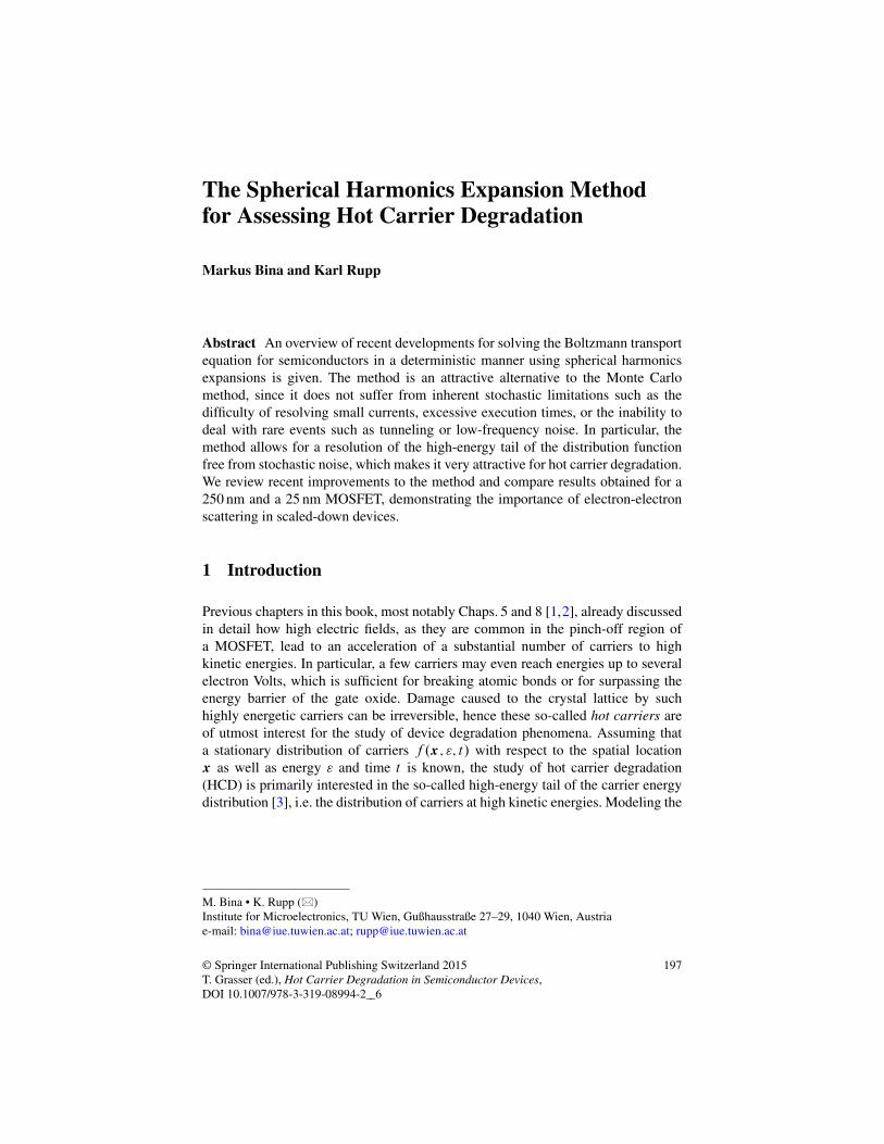
Fig. 1 Exemplary distribution functions and acceleration integrals (shaded area) for electrons

(left) and holes (right) in the middle of an artificial short channel (25 nm) n-channel MOSFET.

The importance of the high-energy tail due to the rapid increase in the collision cross section S."/

for the calculation of the acceleration integral is readily visible

eventual damage caused by a carrier at energy " through a so-called capture cross

section S."/, the total rate G.x; t / is obtained from the acceleration integral (AI)

G.x; t / �

Z 1

0

f .x; "; t/S."/ d":

Typically, the capture cross section is assumed to vanish below a certain threshold

energy "th:

G.x; t / �

Z 1

"th

f .x; "; t/S."/ d"; (1)

Although secondary carrier generation requires a kinetic energy of the primary

particle above the band gap energy, "th generally takes values below the band gap

energy to include effects other than secondary carrier generation. Above "th, the

capture cross section S."/ grows quickly [4]. Thus, the distribution function needs

to be computed accurately at higher energies, which mandates the consideration

of appropriate scattering mechanisms [3, 5] including carrier-carrier scattering and

impact ionization [5,6] (cf. Fig. 1). The remainder of this chapter will thus focus on

the accurate computation of the carrier distribution function, whereas more elaborate

studies of HCD based on the availability of the high-energy tail of the distribution

function can be found especially in Chaps. 5, 7, 10, and 13 [1, 2, 7, 8].

The governing equation for the aforementioned carrier distribution function,

the Boltzmann Transport Equation (BTE), is discussed in Sect. 2. A deterministic

solution method by means of spherical harmonics expansions is then presented in

Sect. 3. The various physical input quantities such as the band structure and the

scattering mechanisms are discussed in detail in Sect. 4. Then, Sect. 5 presents HCD

simulation results for an n-channel MOSFET. A discussion of not only technical

aspects in making the SHE method more accessible to the HCD community is given

in Sect. 6. Finally, this chapter closes with a conclusion in Sect. 7.

The SHE Method for Assessing Hot Carrier Degradation 199

2 The Boltzmann Transport Equation

The BTE describes the carrier transport subject to the collision-less, free flight in

response to an external force, as well as scattering with other carriers or the crystal

lattice. The free flight of charge carriers in the lattice is described by the equations

of motion (Newton’s law)

„@tk0 D F and @tx D v; (2)

where the relation p D „k0 coupling the momentum p with the wave vector

k0 is employed. The collisions between carriers and the lattice is described by

quantum mechanical perturbation theory (Fermi’s Golden Rule). It has to be

noted that in the classical framework of the BTE, where Heisenberg’s uncertainty

principle is neglected, both position and momentum of each carrier can be tracked

precisely. However, tracking each particle individually in a classical approach is

computationally infeasible, therefore the spatial and temporal evolution of particles

is condensed into an ensemble distribution function f .x;k0; t /, which is defined

such that

dN D2

.2�/3f d3x d3k0 (3)

is the number of carriers in the infinitesimal small volume d3x d3k0 in the six-

dimensional phase-space at time t . Without going into the details of the derivation,

the so-defined distribution function obeys the BTE

@f

@tC v · rxf C

1

„F · rk0f D Qff g C �; (4)

where v denotes the group velocity,

F D �rx.q C "b/ (5)

is the force due to the electrostatic potential , the particle charge q (negative for

electrons, positive for holes), and the band edge minimum "b. Qff g refers to the

scattering operator and � models the generation and recombination of carriers.

Magnetic fields can also be included in a straight-forward manner [9], yet will

not be considered further in this work. In principle, a BTE needs to be solved for

each valley and each carrier type (electrons and holes), where interactions occur

through inter-valley scattering and generation-recombination processes. For the sake

of simplicity and better readability, the subsequent discussion assumes a single

valley for a single carrier type unless noted otherwise and arguments are suppressed

whenever appropriate. Since the electrostatic potential is needed in order to

compute the force exerted on each charge carrier, one needs to solve Poisson’s


equation and the BTE for electrons and holes self-consistently. The full system of

equations thus reads

r · .".x/r / D jqj.n � p C C/;

@tfn C vn · rxf

n C „�1F · rkfn

„ ƒ‚ …

DLnff ng

D Qnff ng � �nff n; f pg;

@tfp C vp · rxf

p � „�1F · rkfp

„ ƒ‚ …

DLpff pg

D Qpff pg � �pff n; f pg;

(6)

where f n and f p denote the electron and hole distribution functions, n and p are

the electron and hole concentrations, respectively, and C accounts for fixed charges

such as the doping. Ln and Lp are the so-called free streaming operators for electrons

and holes, describing the free flight of carriers.

Without further approximations, each BTE has to be solved in three spatial

and three phase space dimensions as well as time. As a consequence, a direct

discretization of the full system in such a high-dimensional space results in

prohibitive memory requirements and execution times for most applications. Thus,

further approximations or alternative discretization schemes have to be employed.

The numerical solution of (6) is traditionally approached by using the Monte

Carlo method [10], which is computationally- and time-intensive, particularly when

the high-energy tails of the distribution function have to be resolved in detail [11].

As a consequence, first results obtained using the Monte Carlo method for a long-

channel MOSFET were reported only recently [4]. Therefore, simplified models

not relying on solution of the BTE have been developed in the meanwhile [12, 13],

some of which are discussed in Chaps. 5, 6, 11, and 13 in this book [1, 7, 8, 14].

Moreover, the inherent stochastic noise in the high-energy tail of the distribution

function computed by the Monte Carlo method may introduce significant errors to

the computed rates.

3 Spherical Harmonics Expansion

Macroscopic models obtained from moments of the distribution function are only

poorly suited for research on HCD, because the distribution function is no longer

accessible directly and has to be recovered through assumptions and approxima-

tions. On the other hand, for the reasons discussed in the previous section the

Monte Carlo method suffers from limitations inherent to its stochastic nature when

applied to the study of HCD. Here we consider the spherical harmonics expansion

(SHE) method, which is a deterministic spectral method for solving the BTE and

consequently free of stochastic noise. A resolution of the distribution function over

a virtually arbitrary scale is possible, rendering the method very attractive for HCD.


In the SHE method, the distribution function is expanded into spherical harmon-

ics Y l;m, where the series is truncated at a maximum expansion order lmax [15, 16].

This is motivated by the fact that the distribution of carriers in equilibrium is spheri-

cally symmetric and can thus, unlike moment-based methods, be represented exactly

by a zeroth-order expansion. Moreover, dispersion relations of semiconductors,

particularly silicon, are in good approximation spherical after a suitable scaling of

the principal axes of the phase space. More precisely, the elliptical valleys in silicon

are mapped onto spherical ones using the Herring-Vogt transform [17] (for each

valley)

OT D

0

@

Tx 0 0

0 Ty 0

0 0 Tz

1

A

from the original k0 space to the transformed space via k D OTk0. Consequently,

the partial derivatives in the BTE (4) need to take this transformation into account,

resulting in

@f

@tC OT v · rxf C

1

„OTF · rkf D Qff g (7)

for the Herring-Vogt-transformed case.

A SHE can in principle be carried out for either constant modulus k D kkk of the

transformed wave vector, or for constant kinetic energy ". An expansion with respect

to energy has several advantages: For example, the distribution function is isotropic

on equienergy surfaces in equilibrium and many scattering rates are a function of

energy [18]. Thus, the spherical coordinates .k; �; '/ in k-space are mapped onto

spherical coordinates ."; �; '/ in energy space, where we keep the angles unchanged

and require the mapping to be unique in both directions [19]. Such a one-to-one

mapping is naturally fulfilled for parabolic and nonparabolic models, but not for a

full-band model. However, we will see in Sect. 4.1 that the requirement of a one-to-

one mapping can be relaxed substantially, allowing for the consideration of a broad

range of full-band effects.

An arbitrary function u can be expanded in energy space with spherical coordi-

nates ."; �; '/ as

u.x;k."; �; '/; t/ D

1X

lD0

lX

mD�l

ul;m.x; "; t/Yl;m; (8)

where Y l;m are the orthonormal, real-valued spherical harmonics on the unit sphere.

Conversely, for any given function u on the unit sphere, the expansion coefficient

ul;m is obtained from a projection onto the respective spherical harmonic:

ul;m D

Z

@˝

uY l;m d˝ (9)


Here, ˝ denotes the unit sphere and d˝ D sin � d� d'. The description of the

BTE in k-space requires a projection of a function u to be applied over the whole

Brillouin zone B for a given energy " as

1

.2�/3

Z

B

ı." � ".k//Y l;mu dk; (10)

resulting after a change to spherical variables in

Z

@˝

Y l;muZ."; �; '/ d˝; (11)

where the generalized density of states Z is obtained from the Jacobian of the

coordinate transformation as

Z."; �; '/ Dk2

.2�/3@k

@": (12)

This generalized density of states differs from the conventional density of states by

a factor of 4� , which is obtained in the spherically symmetric case by an integration

over the angles � and '. The important detail in (11) is the generalized density

of states entering the integrand in the course of the projection. If it is taken to be

spherically symmetric, i.e. Z."; �; '/ D Z."/, then (9) and (11) differ only by

a constant factor for a fixed kinetic energy ". On the other hand, a full angular

dependence of Z will lead to unrelated expansion coefficients obtained from (9)

and (11) in general.

Since the distribution function f is a-priori unknown and only known to

fulfill the BTE, a system of equations for the expansion coefficients needs to be

derived from the BTE. This system is obtained by projecting (7) onto the spherical

harmonics Y l;m. For details of the derivation we refer to the literature [18] and

directly state the resulting set of equations:

@gl;m

@[email protected] · Oj l;m/

@"C rx · Oj l;m � OTF · � l;m D Ql;mfgg; (13)

where we set g WD f Z motivated by (11), Oj is the generalized current density

given by

Oj l;m D

Z

@˝

OT vgY l;m d˝; (14)

and

� l;m D

Z

@˝

g

„k

�@Y l;m

@�e� C

1

sin �

@Y l;m

@'e'

�

d˝ (15)


with unit vectors e� and e' in the spherical coordinate system for the � and '

directions, respectively. The projected scattering operatorQl;mfgg will be discussed

below. To better expose the structure of the equations, we combine rx and @=@" to

yield a divergence in .x; "/-space:

@gl;m

@tC rx;" · Qj l;m � OTF · � l;m D Ql;m; (16)

with

Qj l;m D

Oj l;mF · Oj l;m

!

: (17)

Similar to numerical solution techniques based on Fourier series, we substitute a

SHE truncated at finite expansion order l 0max for g as

g �

l 0maxX

l 0D0

l 0X

m0D�l 0

gl 0;m0Y l0;m0

: (18)

As indicated in Fig. 2, values between one and five are common choices for l 0max for

practical purposes. For a more compact notation we employ Einstein’s summation

convention for repeated upper and lower indices to write

Oj l;m D Ovl0;m0

l;m gl 0;m0 ; (19)

� l;m D �l 0;m0

l;m gl 0;m0 ; (20)

with

Ovl0;m0

l;m D

Z

@˝

OT vY l0;m0

Y l;m d˝; (21)

�l 0;m0

l;m D

Z

@˝

Y l0;m0

„k

�@Y l;m

@�e� C

1

sin �

@Y l;m

@'e'

�

d˝: (22)

After splitting the scattering operator into in-scattering and out-scattering contribu-

tions via Qfgg DP

�Q�fggin �Q�fggout for each scattering process identified by

�, a projection and insertion of (18) results in

@gl;m

@tC rx;" · Qj

l 0;m0

l;m gl 0;m0 � F · �l 0;m0

l;m gl 0;m0

DX

�

�

QinIl 0;m0

�Il;m gl 0;m0.x; "� „!�; t / �QoutIl 0;m0

�Il;m gl 0;m0

�

; (23)


10−2

10−1

100

101

1 2 3 4 5 6 7 8 9

Rel

ati

ve

Err

or

(per

cent)

Expansion Order L

Fig. 2 Comparison of the relative error in the collector current of a silicon-germanium heterojunc-

tion bipolar transistor for different SHE orders [20]. First-order expansions show an error of 10 %

compared to an eleventh-order expansion, which may be unacceptable for scaled-down devices

where the (possibly vanishing) inelastic energy transfer involved in the scattering

process identified by � is „!�. Equation (23) defines a system of .lmax C1/2 coupled

first-order partial differential equations with shifted arguments " � „!� for the

in-scattering term to be solved in order to determine the unknown expansion coef-

ficients gl;m. The system is posed in the five-dimensional .x; "; t/-space rather than

the seven-dimensional .x;k; t /-space of the BTE, hence reducing the computational

burden substantially. Moreover, for stationary simulations the solution space reduces

to four dimensions (or three and two dimensions for two- or one-dimensional device

simulations, respectively). This reduction of dimensionality of the computational

domain makes the SHE method particularly attractive.

3.1 Boundary Conditions

The system of equations (23) needs to be supplemented with suitable boundary

conditions in order to fully specify the equation system. At non-contact bound-

aries, homogeneous Neumann boundary conditions are applied just like for the

drift-diffusion system. Similarly, homogeneous Neumann boundary conditions are

applied at the energy boundaries " D 0 and " D "max, if the considered kinetic

energy range for the simulation is limited by some maximum kinetic energy "max.

Scattering processes with initial or final energy outside the considered energy range,

including scatter events to or from the band gap, are suppressed. Early publications


imposed Maxwell–Boltzmann distributions f eq via Dirichlet boundary conditions

of the form

fl;m."/ D

(

f eq WD M exp�

� "kBT

�

; l D m D 0;

0 otherwise:(24)

at the contacts, where kB is the Boltzmann constant, T denotes temperature, and

M is a suitable normalization factor in order to obtain the correct contact carrier

density. While such a thermal equilibrium assumption is reasonable at the inflow

contacts, it leads to boundary layers at the outflow-contact at higher bias [21],

forcing a heated carrier distribution to thermal equilibrium. This deficiency is

addressed by a generation/recombination process with rate

l;m D �gl;m �Zl;mf

eq

l;m

�0; (25)

where Zl;m is the spherical harmonics expansion coefficient of the generalized

density of states, feq

l;m is the .l;m/-th expansion coefficient of the equilibrium

(Maxwell–Boltzmann) distribution as in (24), and �0 is the recombination time

[18, 21]. Here, �0 provides control over the difference between thermal equilibrium

and the computed solution. In the limit �0 ! 0 the Dirichlet boundary condition

(24) is recovered. Practical values for �0 are in the femtosecond range.

A parameter-free improvement of (25) was introduced by Hong et al. [9], where

a surface generation rate of the form

s.k0/ D ��

f eq1Œ0;1/.� OT v · n/C f 1Œ0;1/. OT v · n/

�OT v · n (26)

with outward pointing unit normal vector n at the contact and the Heaviside step

function 1Œ0;1/ was proposed. Here, the first term describes carriers in thermal

equilibrium entering the device ( OT v to point into the device), while the second

term describes the annihilation of heated carriers leaving the device. Such a

boundary condition corresponds to a thermal bath contact as used in Monte Carlo

simulations [10].

3.2 Stabilization and H-Transform

The partial derivatives with respect to the spatial variable x as well as the kinetic

energy " in (23) describe the motion of carriers in free flight. In the absence of

scattering mechanisms, carriers solely gain or lose kinetic energy in reaction to

the force term F , hence the trajectories of carriers in free flight in .x; "/-space

mirror the potential profile throughout the device. Regular discretizations with

respect to the kinetic energy " are unable to trace these trajectories accurately, hence


numerical instabilities show up if no special measures are applied. Rahmat et al.

used a semi-empirical upwind-scheme to stabilize the equations for the simulation

of devices in the micrometer regime [22]. Jungemann et al. applied the maximum

entropy dissipation scheme (MEDS) [23] and obtained good numerical stability

for devices of about 100 nm length. As ballistic transport becomes increasingly

dominant for smaller devices, the so-called H -transformation [24] was considered

in addition to MEDS in [9] and due to its superior numerical stability used in all

subsequent publications. The essence of the H -transformation is to apply a change

of coordinates from kinetic energy " to total energyH D "�q .x/, through which

the derivative with respect to energy in (23) vanishes and one obtains

@gl;m

@tC rx · Oj

l 0;m0

l;m gl 0;m0 � OTF · �l 0;m0

l;m gl 0;m0

DX

�

�

QinIl 0;m0

�Il;m gl 0;m0.x;H � „!�; t / �QoutIl 0;m0

�Il;m gl 0;m0

�

: (27)

For simplicity the variable names were reused, even though all quantities are now

a function of .x;H; t/ instead of .x; "; t/. Carrier trajectories are now given by

constant total energyH and are well resolved when using a regular grid with respect

to the total energy coordinate, cf. Fig. 3. The price to pay for the high numerical

stability is the dependence of the band edge on the potential, hence the simulation

regions for the conduction and valence bands need to be recomputed after each

change of the potential. MEDS applied to the H -transformed equations results in

the multiplication of the equations by a constant, hence can be omitted. On the other

hand, a scaling of the equations in accordance to MEDS results in an M-matrix

property of the system matrix for a first-order SHE method, which simplifies the

solution process and ensures positivity of the solution [9].

Forbidden

H

x

Trajectories

Fig. 3 TheH -transformation results in carrier trajectories under free flight to be given by constant

total energy H . Scattering mechanisms couple the individual trajectories. The shape of the band

edge is determined by the material configuration and the electrostatic potential


4 Physics

During the presentation of the SHE method in Sect. 3 a discussion of additional

material-specific properties or physical details has been set aside wherever possible.

However, such details are essential for predictive device simulation, yet require a

careful analysis to match the underlying material well. In this section we discuss

these details in more depth. Because of its high technological relevance, results are

primarily given for silicon.

4.1 Band Structure

From the dispersion relation ".k/ one can fully describe the ballistic transport of

carriers in a device. More precisely, both the group velocity rx"=„ and the density

of states (12) are directly obtained. During the derivation of the SHE method we

have required that the mapping from " to k is one-to-one, hence the term 1=.„k/

in (27) can be evaluated directly. For the common analytical band structure models,

namely the parabolic band structure

"parabolic.k/ D„2k2

2m�(28)

with effective mass m� and the non-parabolic modification [25, 26]

"0.1C ˛"0/ D„2k2

2m�(29)

these one-to-one mappings are obtained directly. Similarly, the dispersion relation

can be inverted for each band of the many-band model for silicon [27]. These

models typically reproduce the density of states as well as the group velocity fairly

well at energies below 1 eV, but fail to provide good approximations at higher

energies. Thus, they are generally not suitable to assess hot carrier degradation,

where energies above 1 eV are common.

A better approximation of the dispersion relation can in principle be obtained

from a SHE of the inverse dispersion relation

k."; �; '/ D

lkmaxX

lD0

lX

mD�l

kl;mYl;m (30)

for some maximum expansion order lkmax. Such an approach was pursued by Kosina

et al. [19] for the valence band up to an energy of 1.27 eV and later refined by Pham

et al. [28]. Subsequently, a fitted band structure based on the SHE of the conduction


band has also been developed [29]. However, a systematic error cannot be avoided

because of the requirement of a one-to-one-mapping between the kinetic energy "

and the modulus of the wave vector k.

Vecchi et al. [30] found that the equations for a first-order SHE can be recast such

that the term � l;m as defined in (15) does not contribute, hence the explicit one-to-

one mapping is no longer necessary after the projection. Thus, even though such a

one-to-one mapping is formally required for the derivation of the SHE method, one

can directly use full-band data for the modulus of the wave-vector and the density

of states in the final equations. Jin et al. [31] extended this approach to arbitrary-

order expansions by observing that under the assumption of spherically symmetric

dispersion relations one can rewrite

2Z

„kD@vZ

@"(31)

and reuse this to eliminate the explicit dependence on k in (15). With this and the

direct use of full-band data for v and Z as depicted in Fig. 4, good agreement with

results from full-band Monte Carlo simulations was obtained. As a consequence, the

extended Vecchi model is also well-suited for the study of HCD. Hong et al. [16]

proposed a further refinement of this approach in order to eliminate or reduce the

remaining systematic differences in the band description. The key of the derivation

is to postpone the isotropic valley approximation in the approaches by Vecchi et al.

and Jin et al. until the last stage of the model derivation. While the first conduction

band is treated rigorously for increased accuracy, higher conduction bands are

approximated using the isotropic model, leading to a slight overall improvement

in accuracy.

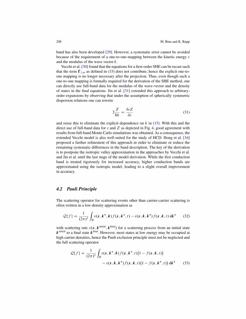
4.2 Pauli Principle

The scattering operator for scattering events other than carrier-carrier scattering is

often written in a low-density approximation as

Qff g D1

.2�/3

Z

B

s.x;k�;k/f .x;k�; t / � s.x;k;k�/f .x;k; t / dk� (32)

with scattering rate s.x;kinitial;kfinal/ for a scattering process from an initial state

kinitial to a final state kfinal. However, most states at low energy may be occupied at

high carrier densities, hence the Pauli exclusion principle must not be neglected and

the full scattering operator

Qff g D1

.2�/3

Z

B

s.x;k�;k/f .x;k�; t /�

1 � f .x;k; t /�

� s.x;k;k�/f .x;k; t /�

1 � f .x;k�; t /�

dk� (33)


0

0.5

1

1.5

2

2.5

3

0 0.5 1 1.5 2 2.5 3 3.5 4

DO

S(1

022

eV−

1cm

−3)

Energy (eV)

ParabolicModena

Many-BandFitted-Band

Full-Band

0

0.5

1

1.5

2

2.5

0 0.5 1 1.5 2 2.5 3 3.5 4

Vel

oci

ty(1

08

cm/s)

Energy (eV)

ParabolicModena

Many-BandFitted-Band

Full-Band

Fig. 4 Comparison of the density of states Z and the group velocity v for different dispersion

relations commonly used with the SHE method

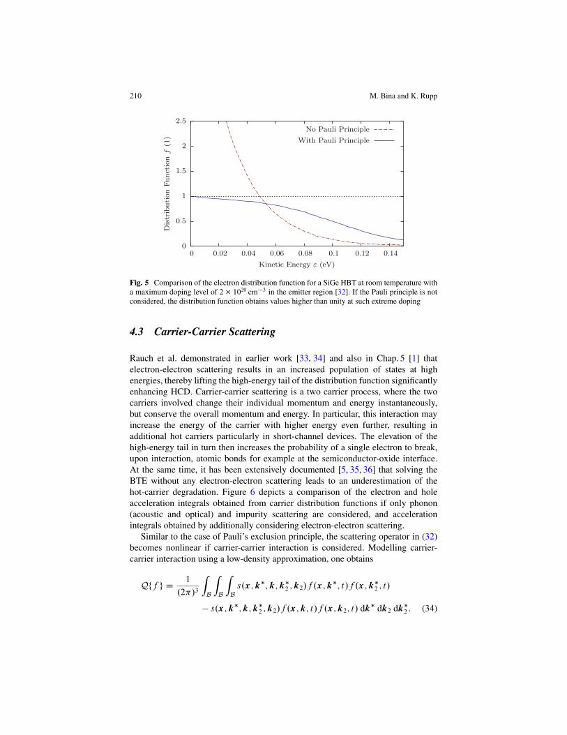
needs to be considered, cf. Fig. 5. As a consequence, the system of SHE equations

becomes nonlinear, which, however, is usually not a concern for self-consistent

simulations, because the SHE equations are already coupled nonlinearly to the

Poisson equation. Hong et al. investigated the influence of Pauli’s exclusion

principle and found a notable difference for doping concentrations only above

1018 cm�3, where the fit factor for impurity scattering needs to be modified in order

to reproduce the Caughey-Thomas expression for the mobility [32].


0

0.5

1

1.5

2

2.5

0 0.02 0.04 0.06 0.08 0.1 0.12 0.14

Dis

trib

ution

Funct

ion

f(1

)

Kinetic Energy ε (eV)

No Pauli Principle

With Pauli Principle

Fig. 5 Comparison of the electron distribution function for a SiGe HBT at room temperature with

a maximum doping level of 2 � 1020 cm�3 in the emitter region [32]. If the Pauli principle is not

considered, the distribution function obtains values higher than unity at such extreme doping

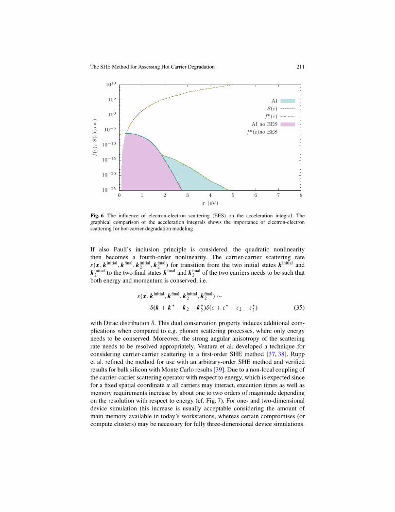
4.3 Carrier-Carrier Scattering

Rauch et al. demonstrated in earlier work [33, 34] and also in Chap. 5 [1] that

electron-electron scattering results in an increased population of states at high

energies, thereby lifting the high-energy tail of the distribution function significantly

enhancing HCD. Carrier-carrier scattering is a two carrier process, where the two

carriers involved change their individual momentum and energy instantaneously,

but conserve the overall momentum and energy. In particular, this interaction may

increase the energy of the carrier with higher energy even further, resulting in

additional hot carriers particularly in short-channel devices. The elevation of the

high-energy tail in turn then increases the probability of a single electron to break,

upon interaction, atomic bonds for example at the semiconductor-oxide interface.

At the same time, it has been extensively documented [5, 35, 36] that solving the

BTE without any electron-electron scattering leads to an underestimation of the

hot-carrier degradation. Figure 6 depicts a comparison of the electron and hole

acceleration integrals obtained from carrier distribution functions if only phonon

(acoustic and optical) and impurity scattering are considered, and acceleration

integrals obtained by additionally considering electron-electron scattering.

Similar to the case of Pauli’s exclusion principle, the scattering operator in (32)

becomes nonlinear if carrier-carrier interaction is considered. Modelling carrier-

carrier interaction using a low-density approximation, one obtains

Qff g D1

.2�/3

Z

B

Z

B

Z

B

s.x;k�;k;k�2 ;k2/f .x;k

�; t /f .x;k�2 ; t /

� s.x;k�;k;k�2 ;k2/f .x;k; t /f .x;k2; t / dk� dk2 dk�

2 : (34)


10−25

10−20

10−15

10−10

10−5

100

105

1010

0 1 2 3 4 5 6 7 8

f(ε

),S(ε

)(a.u

.)

ε (eV)

AI

S(ε)

fn(ε)

AI no EES

fn(ε)no EES

Fig. 6 The influence of electron-electron scattering (EES) on the acceleration integral. The

graphical comparison of the acceleration integrals shows the importance of electron-electron

scattering for hot-carrier degradation modeling

If also Pauli’s inclusion principle is considered, the quadratic nonlinearity

then becomes a fourth-order nonlinearity. The carrier-carrier scattering rate

s.x;kinitial;kfinal;kinitial2 ;kfinal

2 / for transition from the two initial states kinitial and

kinitial2 to the two final states kfinal and kfinal

2 of the two carriers needs to be such that

both energy and momentum is conserved, i.e.

s.x;kinitial;kfinal;kinitial2 ;kfinal

2 / �

ı.k C k� � k2 � k�2 /ı."C "� � "2 � "�

2 / (35)

with Dirac distribution ı. This dual conservation property induces additional com-

plications when compared to e.g. phonon scattering processes, where only energy

needs to be conserved. Moreover, the strong angular anisotropy of the scattering

rate needs to be resolved appropriately. Ventura et al. developed a technique for

considering carrier-carrier scattering in a first-order SHE method [37, 38]. Rupp

et al. refined the method for use with an arbitrary-order SHE method and verified

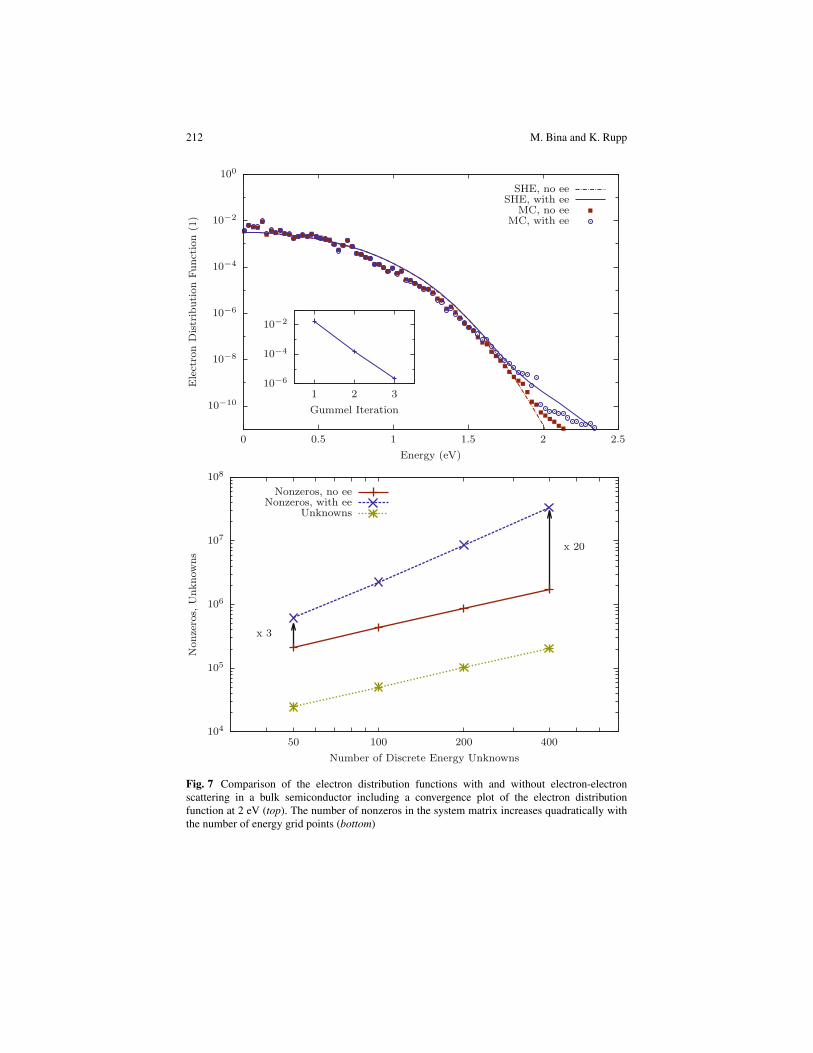
results for bulk silicon with Monte Carlo results [39]. Due to a non-local coupling of

the carrier-carrier scattering operator with respect to energy, which is expected since

for a fixed spatial coordinate x all carriers may interact, execution times as well as

memory requirements increase by about one to two orders of magnitude depending

on the resolution with respect to energy (cf. Fig. 7). For one- and two-dimensional

device simulation this increase is usually acceptable considering the amount of

main memory available in today’s workstations, whereas certain compromises (or

compute clusters) may be necessary for fully three-dimensional device simulations.


10−10

10−8

10−6

10−4

10−2

100

0 0.5 1 1.5 2 2.5

Ele

ctro

nD

istr

ibution

Funct

ion

(1)

Energy (eV)

10−6

10−4

10−2

1 2 3

Gummel Iteration

SHE, no eeSHE, with ee

MC, no eeMC, with ee

104

105

106

107

108

50 100 200 400

Nonze

ros,

Unknow

ns

Number of Discrete Energy Unknowns

x 3

x 20

Nonzeros, no eeNonzeros, with ee

Unknowns

Fig. 7 Comparison of the electron distribution functions with and without electron-electron

scattering in a bulk semiconductor including a convergence plot of the electron distribution

function at 2 eV (top). The number of nonzeros in the system matrix increases quadratically with

the number of energy grid points (bottom)


1 2

r12

r21

neutral

Ener

gy

EC

EV

ET

Gn

Gp

Rn

Rp

negative

∂tfT = (1 − fT)r21 − fTr12

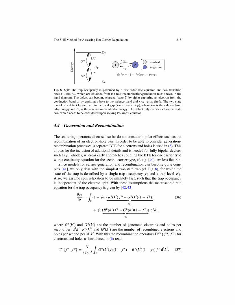
Fig. 8 Left: The trap occupancy is governed by a first-order rate equation and two transition

rates r12 and r21, which are obtained from the four recombination/generation rates shown in the

band diagram. The defect can become charged (state 2) by either capturing an electron from the

conduction band or by emitting a hole to the valence band and vice versa. Right: The two state

model of a defect located within the band gap (EV < ET < EC), where EV is the valence band

edge energy and EC is the conduction band edge energy. The defect only carries a charge in state

two, which needs to be considered upon solving Poisson’s equation

4.4 Generation and Recombination

The scattering operators discussed so far do not consider bipolar effects such as the

recombination of an electron-hole pair. In order to be able to consider generation-

recombination processes, a separate BTE for electrons and holes is used in (6). This

allows for the inclusion of additional details and is needed for fully bipolar devices

such as pn-diodes, whereas early approaches coupling the BTE for one carrier type

with a continuity equation for the second carrier type, cf. e.g. [40], are less flexible.

Since models for carrier generation and recombination can become quite com-

plex [41], we only deal with the simplest two-state trap (cf. Fig. 8), for which the

state of the trap is described by a single trap occupancy fT and a trap level ET.

Also, we assume spin relaxation to be infinitely fast, such that the trap occupancy

is independent of the electron spin. With these assumptions the macroscopic rate

equation for the trap occupancy is given by [42, 43]

@fT

@tD

Z

B

.1 � fT/ .Rn.k0/f n �Gp.k0/.1 � f p//

„ ƒ‚ …

r21

(36)

C fT .Rp.k0/f n �Gn.k0/.1 � f n//

„ ƒ‚ …

r12

d3k0;

where Gn.k0/ and Gp.k0/ are the number of generated electrons and holes per

second per d3k0, Rn.k0/ and Rp.k0/ are the number of recombined electrons and

holes per second per d3k0. With this the recombination operators �p=nff n; f pg for

electrons and holes as introduced in (6) read

�nff n; f pg DNT

.2�/3

Z

B

Gn.k0/fT.1 � f n/ �Rn.k0/.1 � fT/fn d3k0; (37)


�pff n; f pg DNT

.2�/3

Z

B

Gp.k0/.1 � fT/.1 � f p/ �Rp.k0/fTfp d3k0; (38)

where NT is the trap concentration. The recombination rates for electrons and holes

are [43, 44]

Rn.k0/ D �nvn.k0/ and Rp.k0/ D �pvp.k0/; (39)

where �n and �p are experimentally determined capture cross sections and vn and

vp are reaction velocities for electrons and holes, respectively. From the principle of

detailed balance [42, 44] the generation rates are found as

Gn.k0/ D �nvn.k0/ exp

�ET �E.k/

kBT

�

; (40)

Gp.k0/ D �pvp.k0/ exp

�E.k0/ �ET

kBT

�

: (41)

The expansion into spherical harmonics of equations (37) and (38) utilizing the

H-transform results in

�nff n; f pgl;m D NTZn.H/

�

Gn.H/fT.1 � f nl;m/

�Rn.H/.1

Y0;0� fT/f

nl;m

�

/ıl;0ıl;m; (42)

�nff n; f pgl;m D NTZp.H/

�

Gp.H/.1

Y0;0� fT/.1 � f

p

l;m/

�Rp.H/fTfp

l;m

�

ıl;0ıl;m: (43)

With this the full bipolar system is defined. For further results obtained for a

pn-diode we refer the reader to the work by Rupp et al. [45].

5 Hot Carrier Modeling Using the Spherical Harmonics

Expansion Method

In this section we demonstrate time-efficient SHE solutions of the bipolar BTE,

which are then applied to the investigation of HCD in n-channel MOSFETs.

Detailed results in a full HCD context have already been presented in Chap. 8 [2],

hence we merely supplement the results already given there. We solve (6) self-

consistently on unstructured grids using the free open-source, higher-order spherical

harmonics expansion simulator ViennaSHE [45–47]. Full-band effects in silicon are

accounted for using the method suggested by Jin et al. [31]. The scattering mecha-

nisms considered are acoustical and optical phonon scattering, impurity scattering,


impact ionization [10] with secondary carrier generation, and electron-electron

scattering [39]. To assess the damage caused by hot carriers, the acceleration integral

from (1) is recast as

G.xit; t / D

Z 1

"th

f .xit; "; t/S."/ d" D �0

Z 1

"th

f ."/Z."/

�" � "th

1 eV

�p

vg."/

„ ƒ‚ …

DS."/=�0

d";

(44)

and evaluated for electrons and holes along the gate oxide interface at xit. Here, �0 is

the capture cross section, p D 11 is used for a multi-particle process, whereas p D 1

is taken for a single particle process,Z.�/ denotes the density of states (DOS), vg.�/

is the group velocity, and " is the kinetic energy [48, 49]. The acceleration integral

is the kernel of the hot carrier degradation model and is used to describe single-

and multiple-carrier bond dissociation processes [48,50,51]. To simulate the device

degradation in terms of a relative decrease in Id; lin, we use the acceleration integrals

for electrons and holes in our detailed degradation model [51]. Using this approach,

two two-dimensional n-channel MOSFETs with 250 and 25 nm channel lengths

subjected to hot carrier stress at high oxide (� 8 MV=cm) and lateral electric fields

(� 1 MV=cm) are investigated to assess the numerical and physical properties of

the distribution function and the acceleration integral. Interface states generated

at the semiconductor-oxide interface during HCD disturb the electrostatics of the

device and affect the carrier mobility. To incorporate these effects in a self-consistent

manner, the acceleration integral was evaluated and used within our degradation

model [51] to calculate the interface state density Nit at each simulation step.

Additionally, Nit was used for the self-consistent treatment of trapped charges in

every step.

5.1 Evaluation of Computational Costs

In order to show the impact and the relative computational effort of the various

degrees of sophistication, the ‘conventional’ BTE with impurity and phonon

scattering was used as an initial guess for the subsequent simulations. To achieve

accurate and deterministic solutions of the BTE under high-field conditions, the

distribution function was first obtained for low-field conditions, considering only

phonon and impurity scattering. The obtained solution was in a second step used as

an initial guess for the device simulation under high-field conditions, considering

only phonon and impurity scattering. In a third step, these results were used to

solve the BTE under high-field conditions including electron-electron scattering

and impact ionization scattering. Using this procedure, the total simulation time

and memory usage was minimized.

The computational cost in terms of execution time is depicted in Fig. 9, while

memory requirements are shown in Fig. 10. All simulations have been performed


0

20

40

60

80

100

W/o EES and II EES II and EES Total

Sim

ula

tion

Tim

e(m

in) Results from ’W/o EES and II’

used as Initial Guess

L = 250 nmL = 25 nm

Fig. 9 The time needed to compute the distribution functions for two different device lengths L

and the total simulation time. It can be seen that the simulation times without electron-electron

scattering (EES) and impact ionization (II) scattering are larger than for those for additionally

considering EES and II scattering

1

2

3

4

5

6

7

8

9

10

11

12

W/o EES and II EES II and EES

Mem

ory

Usa

ge(G

B)

L = 250 nmL = 25 nm

Fig. 10 The total random access memory used for each case. Whilst the simulations incorporating

only phonon and impurity scattering took longer than the incremental others, they required

considerably less memory (cf. Fig. 9). The most memory was needed for the long channel device

(L D 250 nm), since more mesh points had to be used. Using electron-electron scattering (EES)

results in a significantly higher memory consumption, which is due to the additional coupling

introduced by the non-linear EES operator. In contrast, impact ionization (II) scattering does not

have a notable influence on the simulation time

using all six cores of an AMD Phenom II X6 1090T Processor with a total memory

of 12 GB. From a productivity point of view it is important to emphasize that the

simulation results are obtained within minutes, whereas conventional Monte Carlo

simulations may take up to several orders of magnitude longer.


10−8

10−6

10−4

10−2

100

102

104

106

108

1010

0 50 100 150 200 250

G(a

.u.)

x (nm)

Spacer

Spacer

L = 250 nm

From Source to Drain

I

IEES

IEES, II

Fig. 11 Plot of the acceleration integrals along the gate oxide interface from source to drain for

electrons (blue) and holes (red), computed from a bipolar solution of the BTE comparing phonon

and impurity scattering, impact ionization (II) scattering, and electron-electron scattering (EES) in

a 250 nm n-channel device under hot-carrier stress

10−8

10−6

10−4

10−2

100

102

104

106

108

1010

0 5 10 15 20 25

G(a

.u.)

x (nm)

Spacer

Spacer

L = 25 nm

From Source to Drain

I

IEES

IEES, II

Fig. 12 The acceleration integrals along the gate oxide interface from the source to drain for

electrons (blue) and holes (red) in a 25 nm n-channel device. The influence of electron-electron

scattering (EES) on the acceleration integral (AI) as compared to the AIs for the long channel

device (cf. Fig. 11) is much more significant, whilst the influence of impact ionization (II) is small

5.2 Evaluation of Computational Results

For the short channel device (25 nm) the shift caused by electron-electron scattering

and shown in Fig. 11 is significantly higher close to the source as compared to the

long channel MOSFET (cf. Fig. 12). Impact ionization causes a dramatic increase

in the acceleration integral for electrons in the long channel device (cf. Fig. 11) near

the drain and a slight increase of the a for holes near the source. Since there is not

enough room for the carriers to lose the attained kinetic energy through scattering


processes in the short channel device, a slight increase of the acceleration integral

for electrons near the source and no increase in the acceleration integral for holes is

observed. It is interesting to note that when comparing the case of impact ionization

with electron-electron scattering with the case where impact ionization was not

considered, no further increase in the acceleration integral for electrons close to

the drain is obtained in the short channel device (cf. Fig. 12). This can be attributed

to the short channel, which does not allow the carriers to gain sufficient energy, and

a loss in kinetic energy through electron-electron scattering near the drain.

6 Available Implementations of the SHE Method

From the discussion and results presented in this chapter the SHE method has to

be seen as a major enabler for future, refined research and developments in HCD.

However, when comparing the SHE method with the established drift-diffusion

model or the Monte Carlo method, the substantially higher complexity, both in terms

of the underlying mathematical algorithms and the physical details, are a substantial

hindrance for wide-spread adoption.

Commercial implementations of selected features of the SHE method are

available from Synopsys [52] and Global TCAD Solutions [53]. The closed-source

nature of these software packages is only poorly suited for stimulating further

research on the SHE method because implementation details are not accessible.

For the same reason, they only provide limited extensibility. To mitigate these

problems, our work on the simulator ViennaSHE [54] is freely accessible as open

source software under a permissive MIT/X11 license. In addition to regular releases,

the developer repository is publicly accessible via the web-based hosting service

GitHub [55], simplifying the ability to provide feedback or even code contributions

substantially.

7 Conclusion

The SHE method is attractive for the study of hot carrier degradation, since it

allows for the computation of deterministic solutions of the BTE over many orders

of magnitude and free from stochastic noise. Important details such as impact

ionization and carrier-carrier scattering can be included at a high level of detail,

while simulation times are only in the order of minutes or hours.

Acknowledgements The authors wish to thank P. Palestri and A. Zaka for providing Monte Carlo

data for carrier-carrier scattering. Support by the Austrian Science Fund (FWF), grant P23598, is

gratefully acknowledged.


References

1. S.E. Rauch, F. Guarin, The energy driven hot carrier model, in Hot Carrier Degradation in

Semiconductor Devices, ed. by T. Grasser. (Springer, Cham, 2014)

2. S. Tyaginov, Physics-based modeling of hot-carrier degradation, in Hot Carrier Degradation

in Semiconductor Devices, ed. by T. Grasser. (Springer, Cham, 2014)

3. S. Tyaginov, I. Starkov, C. Jungemann, H. Enichlmair, J. Park, T. Grasser, in Proceedings of

ESSDERC, pp. 151–154 (2011)

4. S. Tyaginov, I. Starkov, O. Triebl, J. Cervenka, C. Jungemann, S. Carniello, J. Park,

H. Enichlmair, M. Karner, C. Kernstock, E. Seebacher, R. Minixhofer, H. Ceric, T. Grasser,

in Proceedings of IPFA, pp. 1–5 (2010)

5. M. Bina, K. Rupp, S. Tyaginov, O. Triebl, T. Grasser, in IEEE International Electron Devices

Meeting (IEDM), pp. 30.5.1–30.5.4 (2012)

6. W. McMahon, A. Haggag, K. Hess, IEEE Trans. Nanotechnol. 2(1), 33 (2003)

7. A. Zaka, P. Palestri, Q. Rafhay, R. Clerc, D. Rideau, L. Selmi, Semi-analytic modeling for

hot carriers in electron devices, in Hot Carrier Degradation in Semiconductor Devices, ed. by

T. Grasser. (Springer, Cham, 2014)

8. S. Reggiani, G. Barone, E. Gnani, A. Gnudi, G. Baccarani, S. Poli, R. Wise, M.Y. Chuang,

W. Tian, S. Pendharkar, M. Denison, Characterization and modeling of high-voltage LDMOS

transistors, in Hot Carrier Degradation in Semiconductor Devices, ed. by T. Grasser. (Springer,

Cham, 2014)

9. S.M. Hong, C. Jungemann, J. Comput. Electron. 8, 225 (2009)

10. C. Jungemann, B. Meinerzhagen, Hierarchical Device Simulation. Computational Microelec-

tronics (Springer, Wien, 2003)

11. B. Meinerzhagen, A. Pham, S.M. Hong, C. Jungemann, in International Conference on

Simulation of Semiconductor Processes and Devices (SISPAD), pp. 293–296 (2010)

12. A. Bravaix, C. Guerin, V. Huard, D. Roy, J. Roux, E. Vincent, in IEEE International Reliability

Physics Symposium, pp. 531–548 (2009)

13. C. Guerin, V. Huard, A. Bravaix, J. Appl. Phys. 105(11), 114513 (2009)

14. A. Bravaix, V. Huard, F. Cacho, X. Federspiel, D. Roy, Hot-carrier degradation in decananome-

ter CMOS nodes: from an energy driven to a unified current degradation modeling by multiple

carrier degradation process, in Hot Carrier Degradation in Semiconductor Devices, ed. by

T. Grasser. (Springer, Cham, 2014)

15. N. Goldsman, C. Lin, Z. Han, C. Huang, Superlattices Microstruct. 27, 159 (2000)

16. S. Hong, A. Pham, C. Jungemann, Deterministic Solvers for the Boltzmann Transport Equation

(Springer, Wien, 2011)

17. C. Herring, E. Vogt, Phys. Rev. 101(3), 944 (1956)

18. C. Jungemann, A.T. Pham, B. Meinerzhagen, C. Ringhofer, M. Bollhöfer, J. Appl. Phys.

100(2), 024502 (2006)

19. H. Kosina, M. Harrer, P. Vogl, S. Selberherr, in Proceedings of SISDEP, pp. 396–399 (1995)

20. S.M. Hong, C. Jungemann, in Proceedings of ESSDERC, pp. 170–173 (2008)

21. D. Schroeder, D. Ventura, A. Gnudi, G. Baccarani, Electron. Lett. 28(11), 995 (1992)

22. K. Rahmat, J. White, D.A. Antoniadis, IEEE Trans. Comput. Aided Des. Integr. Circuits Syst.

15(10), 1181 (1996)

23. C. Ringhofer, Trans. Theory Stat. Phys. 31, 431 (2002)

24. A. Gnudi, D. Ventura, G. Baccarani, F. Odeh, Solid State Electron. 36(4), 575 (1993)

25. R. Brunetti, C. Jacoboni, F. Nava, L. Reggiani, G. Bosman, R. Zijlstra, J. Appl. Phys. 52(11),

6713 (1981)

26. C. Jacoboni, P. Lugli, The Monte Carlo Method for Semiconductor Device Simulation

(Springer, Wien, 1989)

27. R. Brunetti, Solid State Electron. 32, 1663 (1989)

28. A.T. Pham, C. Jungemann, B. Meinerzhagen, in Proceedings of SISPAD, pp. 361–364 (2006)

29. G. Matz, S.M. Hong, C. Jungemann, in Proceedings of SISPAD, pp. 167–170 (2010)


30. M.C. Vecchi, D. Ventura, A. Gnudi, G. Baccarani, in Proceedings of NUPAD, pp. 55–58 (1994)

31. J. Seonghoon, S. Hong, C. Jungemann, IEEE Trans. Electron Devices 58(5), 1287 (2011)

32. S.M. Hong, C. Jungemann, in Proceedings of SISPAD, pp. 135–138 (2010)

33. S. Rauch, F. Guarin, G. La Rosa, IEEE Electron Devices Lett. 19(12), 463 (1998)

34. S. Rauch, G. La Rosa, F. Guarin, IEEE Trans Devices Mater. Reliab. 1(2), 113 (2001)

35. A. Zaka, P. Palestri, Q. Rafhay, R. Clerc, M. Iellina, D. Rideau, C. Tavernier, G. Pananakakis,

H. Jaouen, L. Selmi, IEEE Trans. Electron Devices 59(4), 983 (2012)

36. S. Tyaginov, M. Bina, F. Jacopo, D. Osintsev, Y. Wimmer, B. Kaczer, T. Grasser, in IEEE

International Integrated Reliability Workshop Final Report (2013)

37. A. Ventura, D. Gnudi, , G. Baccarani, in Proceedings of SISDEP, pp. 161–164 (1993)

38. D. Ventura, A. Gnudi, G. Baccarani, F. Odeh, Appl. Math. Lett. 5(3), 85 (1992)

39. K. Rupp, P.W. Lagger, T. Grasser, A. Jungel, in Proceedings of IWCE, pp. 1–4 (2012)

40. H. Lin, N. Goldsman, I.D. Mayergoyz, in Proceedings of IWCE, pp. 143–146 (1992)

41. T. Grasser, Microelectron. Reliab. 52(1), 39 (2012)

42. O. Madelung, Introduction to Solid-State Theory. Springer Series in Solid-State Sciences

(Springer, New York, 1996)

43. A. Piazza, C. Korman, A. Jaradeh, IEEE Trans. Comput. Aided Des. Integr. Circuits Syst.

18(12), 1730 (1999)

44. W. Shockley, W.T. Read, Phys. Rev. 87, 835 (1952)

45. K. Rupp, C. Jungemann, M. Bina, A. Jüngel, T. Grasser, in Proceedings of SISPAD, pp. 19–22

(2012)

46. K. Rupp, T. Grasser, A. Jüngel, in IEDM Technical Digest (2011)

47. K. Rupp, T. Grasser, A. Jüngel, in Proceedings of SISPAD, pp. 151–155 (2011)

48. W. McMahon, A. Haggaag, K. Hess, IEEE Trans. Nanotechnol. 2(1), 33 (2003)

49. S. Tyaginov, I. Starkov, H. Enichlmair, J. Park, C. Jungemann, T. Grasser, ECS Trans. 35(4),

321–352 (2011). Online: http://ecst.ecsdl.org/content/35/4/321.abstract

50. A. Bravaix, V. Huard, in European Symposium on the Reliability of Electron Devices (2010)

51. S. Tyaginov, I. Starkov, O. Triebl, H. Enichlmair, C. Jungemann, J. Park, H. Ceric, T. Grasser,

in Proceedings of SISPAD, pp. 123–126 (2011)

52. Synopsys Inc. Online: http://www.synopsys.com/

53. Global TCAD Solutions. Online: http://www.globaltcad.com/

54. ViennaSHE Device Simulator. Online: http://viennashe.sourceforge.net/

55. ViennaSHE Developer Repositories. Online: http://github.com/viennashe/

Date post:	16-Apr-2020
Category:	Documents
Upload:	others
View:	15 times
Download:	0 times

The Spherical Harmonics Expansion Method for Assessing Hot ... · The Spherical Harmonics Expansion...

Documents