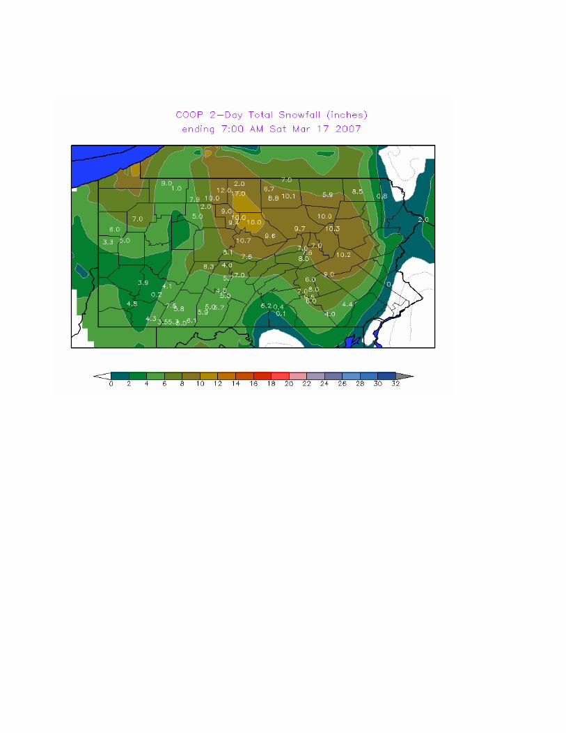
The St Patrick’s Snow Storm of 16-17 March 2007 By

Richard H. Grumm National Weather Service Office State College PA 16803

1. INTRODUCTION A complex March snowstorm struck the eastern United States on 16-17 March 2007. This storm came on the heals of a brief March warm spell and rain event which had produce flooding from Pennsylvania northward into New England. Flooding began on the 15th and was on-going in many locations as the snow began. Snow fall totals ranged from a few inches in Ohio, Maryland, and along the coast to around 2 feet in east-central New York State (Fig. 1). Snow fall in Pennsylvania was heavier from central sections eastward into New Jersey. There were reports of a much as 18 inches of snow in isolated parts of central Pennsylvania. The highest spotter report was 18 inches in northeast Pennsylvania. The Catskills of east-central New York received the most snow with many locations reporting 20-24 inches of snowfall. Snowfall was lower in New England and along the coast. The coastal plain saw periods of freezing rain and ice pellets which limited snowfall over Long Island and southeastern New England. The extent of the snowfall and amounts rank this as a major snow storm and likely the second largest snowstorm of the winter of 2006-2007. The Valentines Day storm affected a larger area and produced upwards to 3 feet of snowfall in New York State.

This storm was relatively well forecast by the NCEP deterministic models and the NCEP ensemble prediction systems. A key caveat being that the potential for snow was in the global ensemble forecast system (GEFS) 3-5 days in advance. However, a well defined cyclone and potential major East Coast storm (ECWS: Hirsch et al 2001) did not appear in the Global Forecast System until the forecasts issued at 1200 UTC 15 March, not surprisingly, the GEFS also began to show a major ECWS at this time. The operational North American Mesoscale Model (NAM) and the short-range ensemble forecast system converged on this storm slower than the global-based system. Thus, in the 1-2 day time range, the storm was a success. In the longer ranges, though snow was in the envelope of solutions, it was not particularly well forecast. Part of this paper will be devoted to forecasts at longer ranges and a terse comparisons in the critical period of 18 to 36 hours before the event. Approximately 36 to 48 hours before the onset of the snow, the guidance began to show a deep cyclone, and anomalous easterly winds at 850 hPa. The easterly wind anomalies have been shown to be critical signal in major ECWS (Stuart and Grumm 2006). Overall, short-range forecasts indicated a major winter storm 24 hours in advance. The highly anomalous low-level jet forecast north of the cyclone raised concerns for 1 to 2 feet of snow potential. The exact location of this band was not clear cut.

Figure 2 NAM 00-hour forecasts initialzied at 0000 UTC 16 March 2007 showing a) mean sea level pressure (hPa) and anomalies (shaded), b) 850 hPa temperatures (C ) and anomalies, c) 850 hPa winds and u-wind anomalies, and d) 850 hPa winds and v-wind anomalies. Anomalies are in standard deviations from the 30 year normals.

Thus, the deterministic models and the EPS showed the potential for banding a concentrated area of heavier snowfall. Another forecast issue was precipitation type. Forecasts from 1200 UTC 15 March 2007 in the GFS and GEFS suggested the rain snow line would push well into Maryland. This raised the potential for heavy snowfall in southern Pennsylvania and central Maryland. The SREF and NAM initially were not as aggressive with the southward surge of cold air. This created precipitation type

issues from south-central Pennsylvania northeastward into southern New England. In addition to the precipitation type issues was snow to liquid ratios. In regions of Pennsylvania, were all EPS members showed snow, the temperatures through most of the storm did not favor dendritic crystals. The 850 and 700 hPa temperatures were forecast to remain in the -4 to -9C range through most of the storm. I most areas, snow to water ratios were biased toward a more traditional

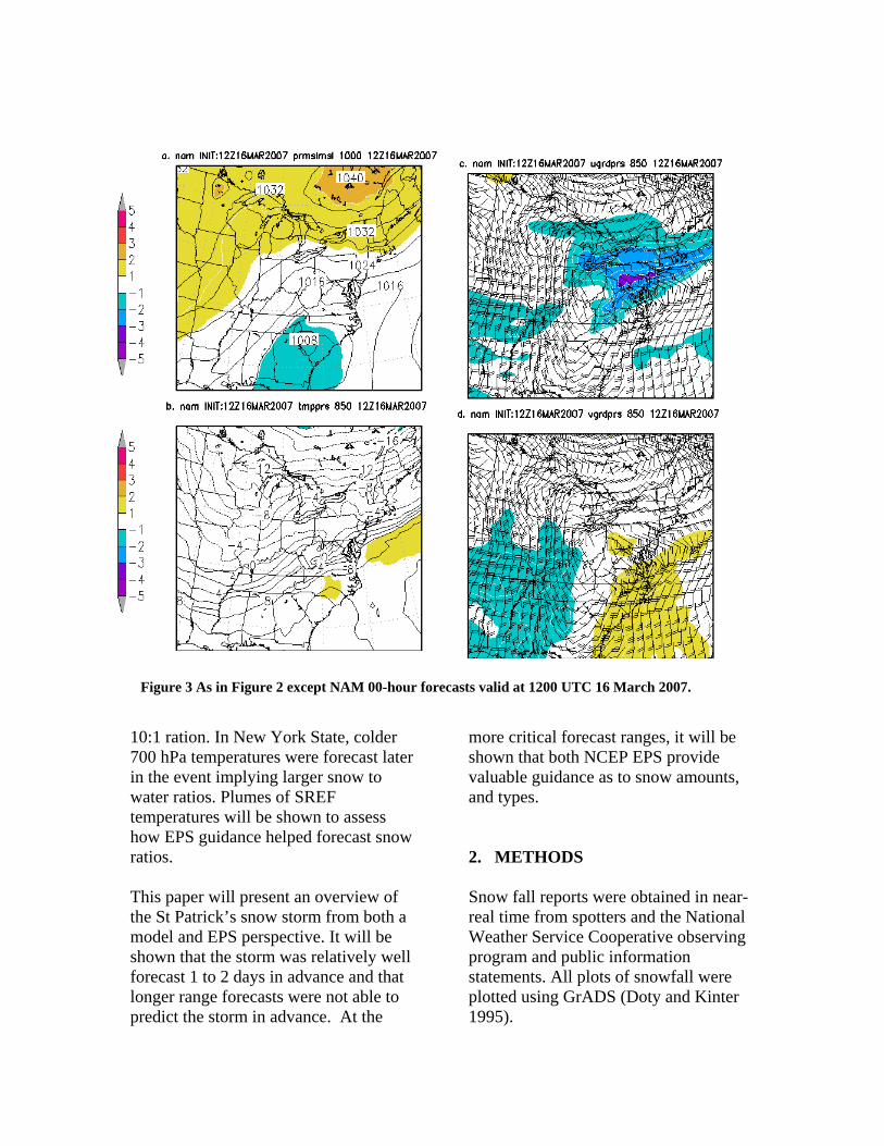
Figure 3 As in Figure 2 except NAM 00-hour forecasts valid at 1200 UTC 16 March 2007.

10:1 ration. In New York State, colder 700 hPa temperatures were forecast later in the event implying larger snow to water ratios. Plumes of SREF temperatures will be shown to assess how EPS guidance helped forecast snow ratios. This paper will present an overview of the St Patrick’s snow storm from both a model and EPS perspective. It will be shown that the storm was relatively well forecast 1 to 2 days in advance and that longer range forecasts were not able to predict the storm in advance. At the

more critical forecast ranges, it will be shown that both NCEP EPS provide valuable guidance as to snow amounts, and types. 2. METHODS Snow fall reports were obtained in near-real time from spotters and the National Weather Service Cooperative observing program and public information statements. All plots of snowfall were plotted using GrADS (Doty and Kinter 1995).

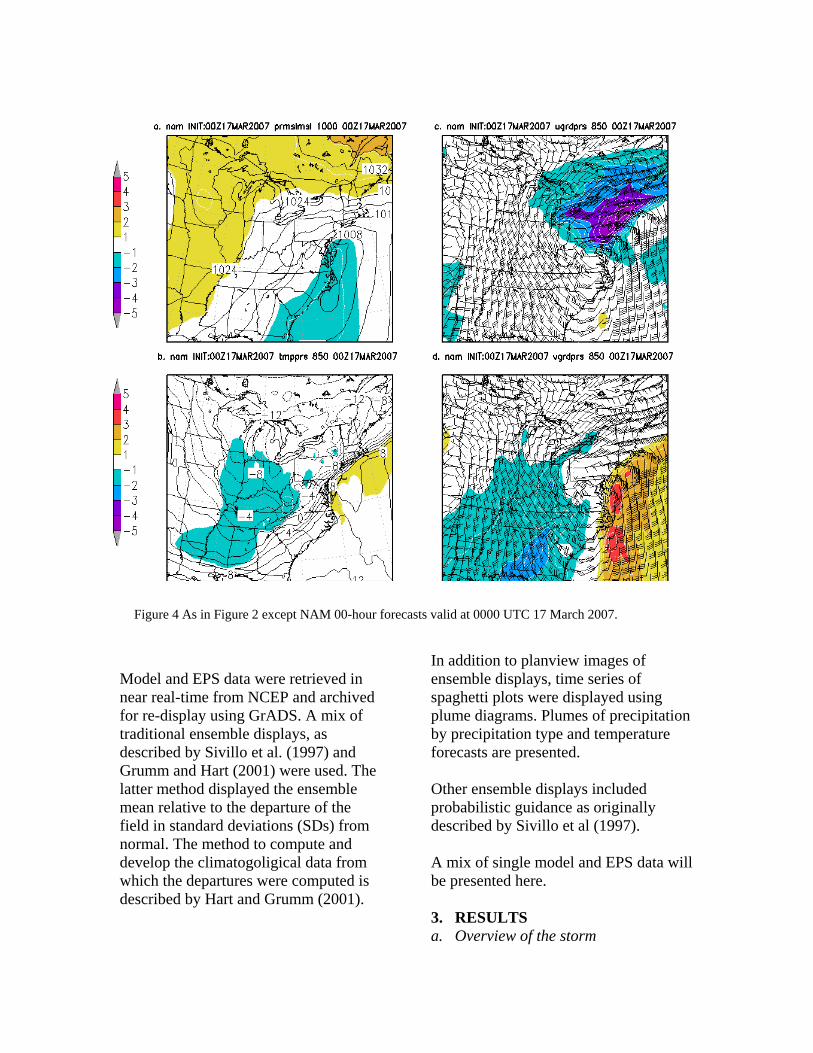
Figure 4 As in Figure 2 except NAM 00-hour forecasts valid at 0000 UTC 17 March 2007.

Model and EPS data were retrieved in near real-time from NCEP and archived for re-display using GrADS. A mix of traditional ensemble displays, as described by Sivillo et al. (1997) and Grumm and Hart (2001) were used. The latter method displayed the ensemble mean relative to the departure of the field in standard deviations (SDs) from normal. The method to compute and develop the climatogoligical data from which the departures were computed is described by Hart and Grumm (2001).

In addition to planview images of ensemble displays, time series of spaghetti plots were displayed using plume diagrams. Plumes of precipitation by precipitation type and temperature forecasts are presented. Other ensemble displays included probabilistic guidance as originally described by Sivillo et al (1997). A mix of single model and EPS data will be presented here. 3. RESULTS a. Overview of the storm

Figure 5 As in Figure 2 except NAM 00-hour forecasts valid at 1200 UTC 17 March 2007.

A large surface anticyclone pushed a cold front into the Mid-Atlantic region on the 15th. In many locations the rain turned to snow as the cold air pushed southward. The surface features, 850 hPa temperatures, and 850 hPa winds at 16/0000 UTC are shown in Figure 2. A strong surface anticyclone with mean sea level pressure values near 1032 hPa were over the lakes. The 850 hPa cold front extended from near Cape Cod westward into Tennessee. A strong easterly wind and anomaly had developed over the

Midwest with anomalies on the order of -2.5SDs below normal. By 16/1200 UTC the NAM analysis showed (Fig. 3) a weak surface cyclone over the Carolina’s and a massive anticyclone just north of New England. The 850 hPa cold front had pushed into the southeastern United States. Some classic cold-air damming features were present in the isotherms and pressure fields. Notable the cool surge over the Appalachians and ridging along the coastal plain. North of the cyclone, a strong easterly jet was present with

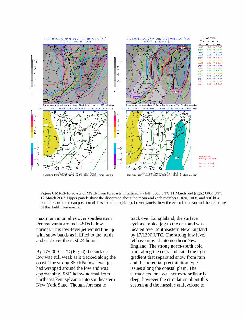
Figure 6 MREF forecasts of MSLP from forecasts initialized at (left) 0000 UTC 11 March and (right) 0000 UTC 12 March 2007. Upper panels show the dispersion about the mean and each members 1020, 1008, and 996 hPa contours and the mean position of these contours (black). Lower panels show the ensemble mean and the departure of this field from normal.

maximum anomalies over southeastern Pennsylvania around -4SDs below normal. This low-level jet would line up with snow bands as it lifted to the north and east over the next 24 hours. By 17/0000 UTC (Fig. 4) the surface low was still weak as it tracked along the coast. The strong 850 hPa low-level jet had wrapped around the low and was approaching -5SD below normal from northeast Pennsylvania into southeastern New York State. Though forecast to

track over Long Island, the surface cyclone took a jog to the east and was located over southeastern New England by 17/1200 UTC. The strong low level jet have moved into northern New England. The strong north-south cold front along the coast indicated the tight gradient that separated snow from rain and the potential precipitation type issues along the coastal plain. The surface cyclone was not extraordinarily deep; however the circulation about this system and the massive anticyclone to

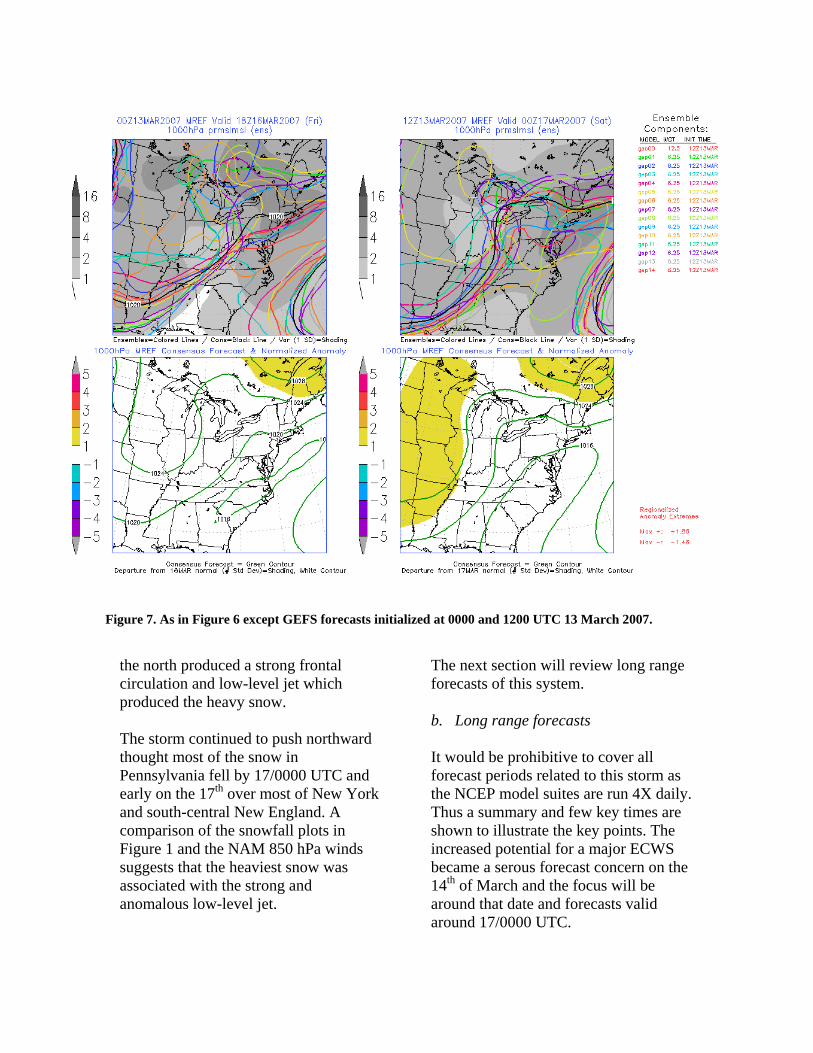
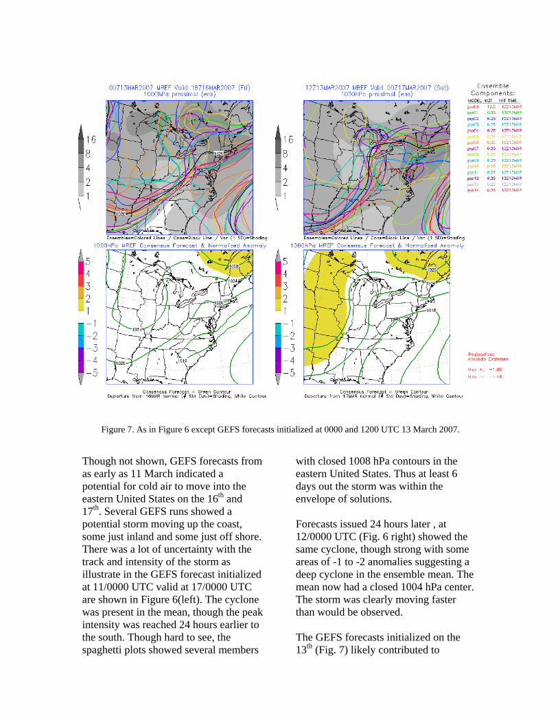
Figure 7. As in Figure 6 except GEFS forecasts initialized at 0000 and 1200 UTC 13 March 2007.

the north produced a strong frontal circulation and low-level jet which produced the heavy snow. The storm continued to push northward thought most of the snow in Pennsylvania fell by 17/0000 UTC and early on the 17th over most of New York and south-central New England. A comparison of the snowfall plots in Figure 1 and the NAM 850 hPa winds suggests that the heaviest snow was associated with the strong and anomalous low-level jet.

The next section will review long range forecasts of this system. b. Long range forecasts It would be prohibitive to cover all forecast periods related to this storm as the NCEP model suites are run 4X daily. Thus a summary and few key times are shown to illustrate the key points. The increased potential for a major ECWS became a serous forecast concern on the 14th of March and the focus will be around that date and forecasts valid around 17/0000 UTC.

Figure 7. As in Figure 6 except GEFS forecasts initialized at 0000 and 1200 UTC 13 March 2007.

Though not shown, GEFS forecasts from as early as 11 March indicated a potential for cold air to move into the eastern United States on the 16th and 17th. Several GEFS runs showed a potential storm moving up the coast, some just inland and some just off shore. There was a lot of uncertainty with the track and intensity of the storm as illustrate in the GEFS forecast initialized at 11/0000 UTC valid at 17/0000 UTC are shown in Figure 6(left). The cyclone was present in the mean, though the peak intensity was reached 24 hours earlier to the south. Though hard to see, the spaghetti plots showed several members

with closed 1008 hPa contours in the eastern United States. Thus at least 6 days out the storm was within the envelope of solutions. Forecasts issued 24 hours later , at 12/0000 UTC (Fig. 6 right) showed the same cyclone, though strong with some areas of -1 to -2 anomalies suggesting a deep cyclone in the ensemble mean. The mean now had a closed 1004 hPa center. The storm was clearly moving faster than would be observed. The GEFS forecasts initialized on the 13th (Fig. 7) likely contributed to

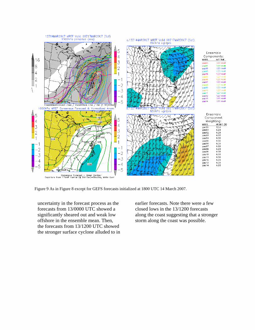
Figure 9 As in Figure 8 except for GEFS forecasts initialized at 1800 UTC 14 March 2007.

uncertainty in the forecast process as the forecasts from 13/0000 UTC showed a significantly sheared out and weak low offshore in the ensemble mean. Then, the forecasts from 13/1200 UTC showed the stronger surface cyclone alluded to in

earlier forecasts. Note there were a few closed lows in the 13/1200 forecasts along the coast suggesting that a stronger storm along the coast was possible.

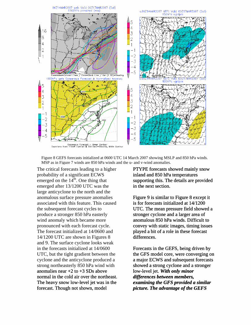
Figure 8 GEFS forecasts initialized at 0600 UTC 14 March 2007 showing MSLP and 850 hPa winds. MSP as in Figure 7 winds are 850 hPa winds and the u- and v-wind anomalies.

The critical forecasts leading to a higher probability of a significant ECWS emerged on the 14th. One thing that emerged after 13/1200 UTC was the large anticyclone to the north and the anomalous surface pressure anomalies associated with this feature. This caused the subsequent forecast cycles to produce a stronger 850 hPa easterly wind anomaly which became more pronounced with each forecast cycle. The forecast initialized at 14/0600 and 14/1200 UTC are shown in Figures 8 and 9. The surface cyclone looks weak in the forecasts initialized at 14/0600 UTC, but the tight gradient between the cyclone and the anticyclone produced a strong northeasterly 850 hPa wind with anomalies near +2 to +3 SDs above normal in the cold air over the northeast. The heavy snow low-level jet was in the forecast. Though not shown, model

PTYPE forecasts showed mainly snow inland and 850 hPa temperatures supporting this. The details are provided in the next section.

anomalies near +2 to +3 SDs above normal in the cold air over the northeast. The heavy snow low-level jet was in the forecast. Though not shown, model

PTYPE forecasts showed mainly snow inland and 850 hPa temperatures supporting this. The details are provided in the next section. Figure 9 is similar to Figure 8 except it is for forecasts initialized at 14/1200 UTC. The mean pressure field showed a stronger cyclone and a larger area of anomalous 850 hPa winds. Difficult to convey with static images, timing issues played a bit of a role in these forecast differences.

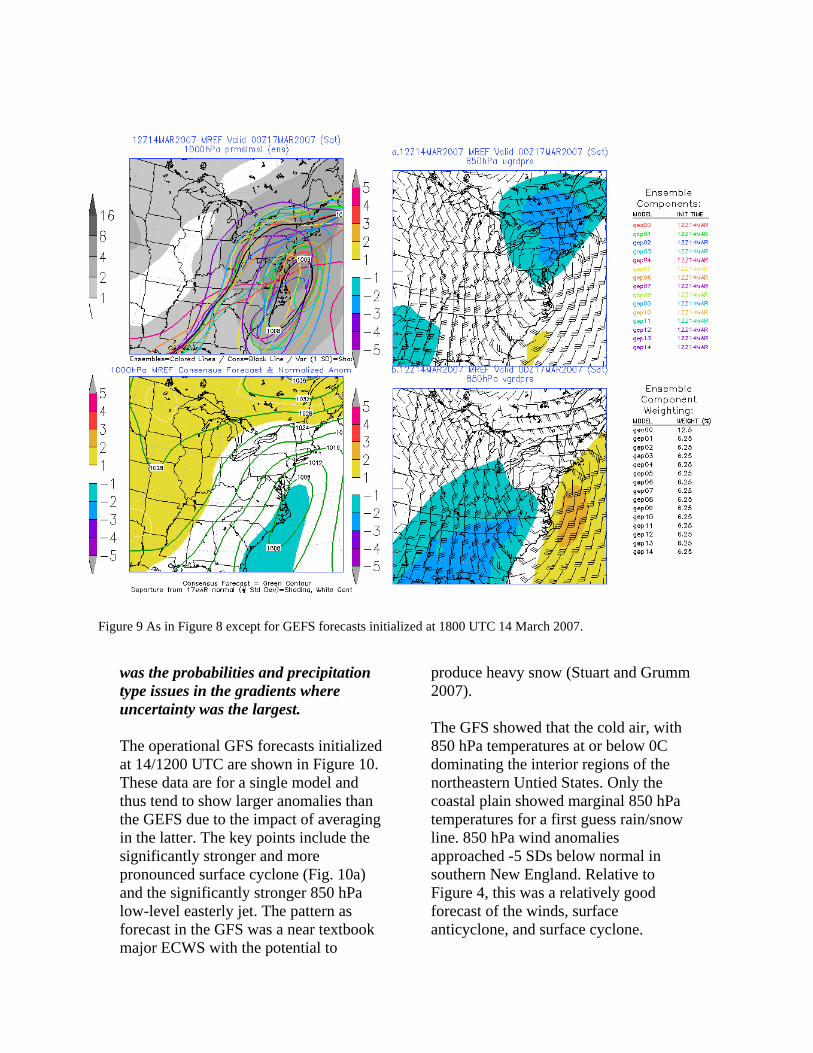
Figure 9 is similar to Figure 8 except it is for forecasts initialized at 14/1200 UTC. The mean pressure field showed a stronger cyclone and a larger area of anomalous 850 hPa winds. Difficult to convey with static images, timing issues played a bit of a role in these forecast differences. Forecasts in the GEFS, being driven by the GFS model core, were converging on a major ECWS and subsequent forecasts showed a strong cyclone and a stronger low-level jet. With only minor differences between members, examining the GFS provided a similar picture. The advantage of the GEFS

Forecasts in the GEFS, being driven by the GFS model core, were converging on a major ECWS and subsequent forecasts showed a strong cyclone and a stronger low-level jet. With only minor differences between members, examining the GFS provided a similar picture. The advantage of the GEFS

Figure 9 As in Figure 8 except for GEFS forecasts initialized at 1800 UTC 14 March 2007.

was the probabilities and precipitation type issues in the gradients where uncertainty was the largest. The operational GFS forecasts initialized at 14/1200 UTC are shown in Figure 10. These data are for a single model and thus tend to show larger anomalies than the GEFS due to the impact of averaging in the latter. The key points include the significantly stronger and more pronounced surface cyclone (Fig. 10a) and the significantly stronger 850 hPa low-level easterly jet. The pattern as forecast in the GFS was a near textbook major ECWS with the potential to

produce heavy snow (Stuart and Grumm 2007). The GFS showed that the cold air, with 850 hPa temperatures at or below 0C dominating the interior regions of the northeastern Untied States. Only the coastal plain showed marginal 850 hPa temperatures for a first guess rain/snow line. 850 hPa wind anomalies approached -5 SDs below normal in southern New England. Relative to Figure 4, this was a relatively good forecast of the winds, surface anticyclone, and surface cyclone.

Figure 10 GFS forecasts initialized at 1200 UTC 14 March 2007 valid at 0000 UTC 17 March 2007 showing a) MSLP and anomalies, b) 850 hPa temperatures and anomalies, c) 850 hPa winds and u-wind anomalies, and d) 850 hPa winds and v-wind anomalies.

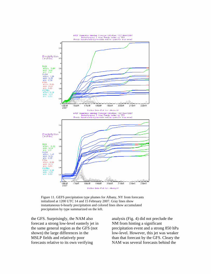
Not surprisingly the model PTYPE showed snow over interior regions and heavy snow at that. A GEFS based plume for Albany New York (Fig. 11) put the snow forecast in perspective. Most members showed snow on the 16th and 17th with the mean near 1.12 of the QPF falling as snow and a few members showing over 2.0 inches of the QPF falling as snow. The GFS and its ensemble spawn, the GEFS, honed in nicely on the storm and were consistent. Had the focus of all

forecasts been on the GFS/GEFS from 14/1200 UTC higher confidence forecasts with better lead-times could have been produced. Lingering uncertainty with the NAM and SREF impacted the forecasts as shown in the next section. c. Short range forecasts The NAM forecasts initialized at 14/1200 UTC valid at 17/0000 UTC is shown in Figure 12. These data imply a weaker cyclone than that produced by

Figure 11. GEFS precipitation type plumes for Albany, NY from forecasts initialized at 1200 UTC 14 and 15 February 2007. Gray lines show instantaneous 6-hourly precipitation and colored lines show accumulated precipitation by type summarized on the left.

the GFS. Surprisingly, the NAM also forecast a strong low-level easterly jet in the same general region as the GFS (not shown) the large differences in the MSLP fields and relatively poor forecasts relative to its own verifying

analysis (Fig. 4) did not preclude the NM from hinting a significant precipitation event and a strong 850 hPa low-level. However, this jet was weaker than that forecast by the GFS. Cleary the NAM was several forecasts behind the

Figure 12 NAM forecasts initialized at 1200 and 1800 UTC 14 March showing forecasts valid at 0000 UTC 17 March of top panels MSLP and lower panels 850 hPa temperatures.

GFS and GEFS in predicting this storm and the NAM is an essential component of the SREF which was equally slow at converging on the solution of a major ECWS. The SREF and NAM did not converge on a solution like the GFS and GEFF until the 15th of March. Figures 13 and 14 show SREF forecasts of MSLP and 850 hPa winds valid at 17/0000 UTC from forecasts initialized at 15/0300 and 15/0900 UTC. The SREF was slowly converging on the solution alluded to by the GFS/GEFS on the 14th with a stronger 850 hPa low-level easterly jet and a more defined surface cyclone and anticyclone. It is unclear

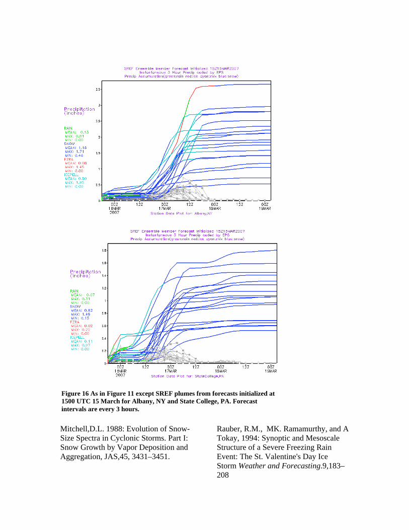
why the SREF and NAM took so long to arrive at these forecasts. By forecasts issued at 15/1500 UTC the SREF appeared to a firm grasp on the storm and the potential for a highly anomalous 850 hPa easterly jet. A series of these forecasts is shown in Figure 15. The SREF forecasts were coming in line with the GFS and GEFS forecasts (not shown). Plumes for Albany, NY and State College, PA are shown in Figure 16. These data show that both locations were forecast to see a mean QPF of around 1.12 and 0.82 inches of liquid which

would fall as snow. State College received about 8 inches of snow locally and about 0.75 inches of liquid equivalent. The Albany area received 11 to 15 inches of snow. Interestingly, after the cold frontal precipitation on the 15th, snow was the only concern at State College with the ECWS on the 16th and 17th. The SREF, unlike the GEFS, had some PTYPE issues at Albany. PTYPE issues would be of concern in the State College forecast area in the southeastern regions. For other forecast offices this problem persisted from Philadelphia, across Long Island and into southern New England. In the coastal plain region, the SREF forecasts were warmer than the GEFS forecasts. As an example, at Middletown, PA (KMDT) the GEFS indicated mainly snow, in fact for the event on the 17th the GEFS showed only snow or ice pellets. The rain was forecast earlier with the event ending on the 15th. Despite the differences, the mean amount of QPF to fall as snow was about the same. But the colder GFS forecast a higher probability of snow and ice pellets than did the SREF, which had several warm members forecasting rain. This precipitation type issue could be shown for many other locations. d. Snow bands Figure 18 shows select composite radar images of the snowbands late on the 16th and 17th. These data show that the intense bands with the strong low-level easterly wind anomalies were well forecast. The anticipated concentrated areas of 1 to 2 feet of snow fell in close proximity to the highly anomalous low-

level 850 hPa jet as shown in the NAM 00-hour forecasts in Figure 2-5. 4. CONCLUSIONS From a short-term forecasting perspective, a well forecast ECWS struck the Mid-Atlantic and Northeastern United States on 16-17 March 2007. The “St Patrick’s” storm of 2007 shared many characteristics common to ECWS. The key feature, with storms producing snowfall in the 1 to 2 foot range includes an anomalous low-level jet. As shown in the NAM analyses, this storm packed a very strong low-level jet which approached -5SD’s below normal at times. The details on the strong low-level jet and the significant ECWS were initially not well forecast by the NAM and SREF relative to the GFS/GEFS. Not all ECWS require an anomalously deep surface cyclone. Similar to the Presidents Weekend storm of February 2003, this event was not associated with a particularly strong and anomalous surface cyclone. The deep cyclone with the Valentine’s Day storm of February 2007 might offer a contrasting event as it was associated with a deep surface cyclone. This storm was driven by a modest surface cyclone and a massive anticyclone to the north. This led to a strong baroclinic zone and very anomalous easterly flow on the cold side of the cyclone. As shown, the region of intense and overall, most significant snowfall was associated with this easterly wind anomaly. Easterly wind anomalies continue to provide useful guidance in anticipating areas of banding and potentially heavy snow fall as indicated by Stuart and Grumm (2007).

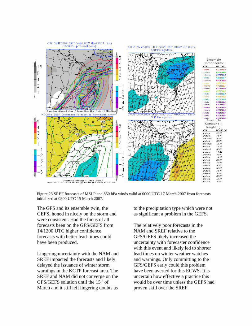
Figure 23 SREF forecasts of MSLP and 850 hPa winds valid at 0000 UTC 17 March 2007 from forecasts initialized at 0300 UTC 15 March 2007.

The GFS and its ensemble twin, the GEFS, honed in nicely on the storm and were consistent. Had the focus of all forecasts been on the GFS/GEFS from 14/1200 UTC higher confidence forecasts with better lead-times could have been produced. Lingering uncertainty with the NAM and SREF impacted the forecasts and likely delayed the issuance of winter storm warnings in the KCTP forecast area. The SREF and NAM did not converge on the GFS/GEFS solution until the 15th of March and it still left lingering doubts as

to the precipitation type which were not as significant a problem in the GEFS. The relatively poor forecasts in the NAM and SREF relative to the GFS/GEFS likely increased the uncertainty with forecaster confidence with this event and likely led to shorter lead times on winter weather watches and warnings. Only committing to the GFS/GEFS early could this problem have been averted for this ECWS. It is uncertain how effective a practice this would be over time unless the GEFS had proven skill over the SREF.

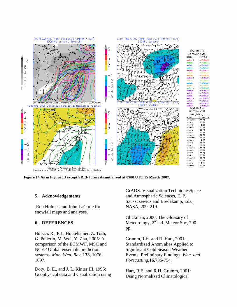
Figure 14 As in Figure 13 except SREF forecasts initialized at 0900 UTC 15 March 2007.

5. Acknowledgements Ron Holmes and John LaCorte for snowfall maps and analyses. 6. REFERENCES Buizza, R., P.L. Houtekamer, Z. Toth, G. Pellerin, M. Wei, Y. Zhu, 2005: A comparison of the ECMWF, MSC and NCEP Global ensemble prediction systems. Mon. Wea. Rev. 133, 1076-1097. Doty, B. E., and J. L. Kinter III, 1995: Geophysical data and visualization using

GrADS. Visualization TechniquesSpace and Atmospheric Sciences, E. P. Szuszczewicz and Bredekamp, Eds., NASA, 209–219. Glickman, 2000: The Glossary of Meteorology, 2nd ed. Meteor.Soc, 790 pp. Grumm,R.H. and R. Hart, 2001: Standardized Anom alies Applied to Significant Cold Season Weather Events: Preliminary Findings. Wea. and Forecasting,16,736-754. Hart, R.E. and R.H. Grumm, 2001: Using Normalized Climatological

Anomalies to Rank Synoptic-Scale Events Objectively. Mon. Wea. Rev.,129,2426-2442. Hirsch,M.eE.,A.T.DeGaetano, and S.J.

Colucci 2001: An East Coast Winter storm climatology. J.Climate,15,882--899.

Colucci 2001: An East Coast Winter storm climatology. J.Climate,15,882--899. Hutchinson, T.A. 1995: An analysis of the NMC’s nested grib model forecasts of Albert Clippers. Wea. Forecasting,10,632-641.

Kocin, P. J., and L. W. Uccellini, 1990: Snowstorms along the Northeastern Coast of the United States: 1955–1985. Meteor. Monogr., No. 44, Amer. Meteor. Soc., 280 pp.

Kocin, P. J., and L. W. Uccellini, 1990: Snowstorms along the Northeastern Coast of the United States: 1955–1985. Meteor. Monogr., No. 44, Amer. Meteor. Soc., 280 pp.

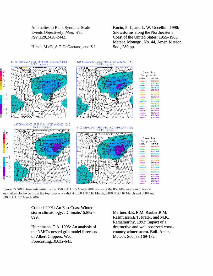
Figure 35 SREF forecasts initialized at 1500 UTC 15 March 2007 showing the 850 hPa winds and U-wind anomalies clockwise from the top forecasts valid at 1800 UTC 16 March, 2100 UTC 16 March and 0000 and 0300 UTC 17 March 2007.

Martner,B.E, R.M. Rauber,R.M. Rasmussen,E.T. Prater, and M.K. Ramamurthy, 1992: Impact of a destructive and well observed cross-country winter storm. Bull. Amer. Meteor. Soc.,73,169-172.

Martner,B.E, R.M. Rauber,R.M. Rasmussen,E.T. Prater, and M.K. Ramamurthy, 1992: Impact of a destructive and well observed cross-country winter storm. Bull. Amer. Meteor. Soc.,73,169-172.

Hutchinson, T.A. 1995: An analysis of the NMC’s nested grib model forecasts of Albert Clippers. Wea. Forecasting,10,632-641.

Figure 16 As in Figure 11 except SREF plumes from forecasts initialized at 1500 UTC 15 March for Albany, NY and State College, PA. Forecast intervals are every 3 hours.

Mitchell,D.L. 1988: Evolution of Snow-Size Spectra in Cyclonic Storms. Part I: Snow Growth by Vapor Deposition and Aggregation, JAS,45, 3431–3451.

Rauber, R.M., MK. Ramamurthy, and A Tokay, 1994: Synoptic and Mesoscale Structure of a Severe Freezing Rain Event: The St. Valentine's Day Ice Storm Weather and Forecasting.9,183–208

Root,B., P Knight,G.Young, S. Greybush,R.Grumm, and R.Holmes, and J.Ross: A Fingerprinting Technique for Major Weather Events. Jour. of Applied Meteorology and Climatology. To appear 2007.

J.Ross: A Fingerprinting Technique for Major Weather Events. Jour. of Applied Meteorology and Climatology. To appear 2007.

Figure 17 Plume diagrams for Harrisburg/Middletown PA. Upper panel shows the 1500 UTC SRF forecast and the lower panel shows the 1200 UTC GEFS forecasts.

Thomas, B.C. and J. Martin 2006: A synoptic climatology and composite analysis of the Alberta Clipper.Wea. Fore.’ Sivillo, S.K,J.E. Ahlquist, and Z. Toth,1997: An ensemble forecasting primer. Wea. Forecasting.,12, 809-818

Thomas, B.C. and J. Martin 2006: A synoptic climatology and composite analysis of the Alberta Clipper.Wea. Fore.’

Sivillo, S.K,J.E. Ahlquist, and Z. Toth,1997: An ensemble forecasting primer. Wea. Forecasting.,12, 809-818

Stensrud D. J., H. E. Brooks, J. Du, M. S. Tracton, and E. Rogers, 1999:

Using Ensembles for Short-Range Forecasting, Mon. Wea. Rev., 127, 433- 446.

Figure 4 Snow fall reports from 17 and 18 March most of the snow fell from late on the 16th into the 17th in New England. Due to UTC times the snow was on the 16th and 17th.

Stewart,R.E. 1992:Precipitation Types in the Transition Region of Winter Storms,BAMS,73,287-296.

Stuart,N.A and R.H. Grumm 2006: Using Wind Anomalies to Forecast East Coast Winter Storms.Wea. and Forecasting,21,952-968. Toth, Z., and Kalnay, E., 1997: Ensemble forecasting at NCEP and the breeding method. Mon. Wea. Rev., 125, 3297-3319. Toth, Z., E. Kalnay, S. M. Tracton, R. Wobus and J. Irwin, 1997: A synoptic evaluation of the NCEP ensemble. Weather and Forecasting, 12, 140-153.

Figure 18. Select composite radar images showing the precipitation shield on 16-17 March at a) 2038 UTC and b) 2228 UTC 16 March and c) 0218 UTC 17 March 2007.