1 THE STOCKHOLM TOLL : AN ECONOMIC EVALUATION 1 Rémy Prud’homme and Pierre Kopp 2 September 7, 2006 Abstract – The Stockholm toll causes, as predicted by theory, a reduction in traffic, leading to increased speeds, and to time gains for remaining car-users. These gains, calculated to be about +110 M. SEK per year, appear to be modest, much lower than similar gains estimated in London, because congestion was moderate and reducing it to its optimal level, which is what the toll achieves, does not represent large increases in speed. The toll also causes environmental benefits, for an estimated +102 M SEK per year. On the other hand, the toll causes a loss for evicted car-users, for about -66 M. SEK per year. A major cost is the implementation cost, about half the cost experienced in London, but nevertheless high at about -730 M SEK per year. Finally, the toll made it necessary in order to accommodate modal shifters to increase public transport supply, at a cost of - 580 M SEK per year, although this increase in public transport supply was not sufficient to prevent a deterioration in service quality tentatively estimated to be above 200 M SEK per year. Overall, costs outweigh the very real benefits of the toll by more than one billion SEK per year. For an urban toll to produce net benefits, it seems that three conditions are required: a relatively high degree of congestion, a reasonably cheap implementation system, and a public transport system with a low marginal cost. 1 This research was made possible by a grant from the research fund (PREDIT) of the French ministry of Transportation. It also benefited from technical assistance from the Swedish Institute for Transport and Communications Analysis (SIKA). The authors are grateful to both entities for their help. They particularly wish to thank Rickard Wall, of SIKA, and Mats Tjernkvist, of Vagverket Konsult, for their kind help. Obviously, our analysis and conclusions do not commit PREDIT or SIKA. 2 Respectively Professor emeritus, University Paris XII and Professor, University Paris I (Sorbonne)
Transcript
1
THE STOCKHOLM TOLL : AN ECONOMIC EVALUATION1
Rémy Prud’homme and Pierre Kopp2
September 7, 2006
Abstract – The Stockholm toll causes, as predicted by theory, a reduction in traffic, leading to increased speeds, and to time gains for remaining car-users. These gains, calculated to be about +110 M. SEK per year, appear to be modest, much lower than similar gains estimated in London, because congestion was moderate and reducing it to its optimal level, which is what the toll achieves, does not represent large increases in speed. The toll also causes environmental benefits, for an estimated +102 M SEK per year. On the other hand, the toll causes a loss for evicted car-users, for about -66 M. SEK per year. A major cost is the implementation cost, about half the cost experienced in London, but nevertheless high at about -730 M SEK per year. Finally, the toll made it necessary in order to accommodate modal shifters to increase public transport supply, at a cost of -580 M SEK per year, although this increase in public transport supply was not sufficient to prevent a deterioration in service quality tentatively estimated to be above 200 M SEK per year. Overall, costs outweigh the very real benefits of the toll by more than one billion SEK per year. For an urban toll to produce net benefits, it seems that three conditions are required: a relatively high degree of congestion, a reasonably cheap implementation system, and a public transport system with a low marginal cost.
1 This research was made possible by a grant from the research fund (PREDIT) of the French ministry of Transportation. It also benefited from technical assistance from the Swedish Institute for Transport and Communications Analysis (SIKA). The authors are grateful to both entities for their help. They particularly wish to thank Rickard Wall, of SIKA, and Mats Tjernkvist, of Vagverket Konsult, for their kind help. Obviously, our analysis and conclusions do not commit PREDIT or SIKA. 2 Respectively Professor emeritus, University Paris XII and Professor, University Paris I (Sorbonne)
2
I – Introduction
On January 2006, the municipality of Stockholm introduced a charge or toll to enter the city center. The main purpose of the charge is to reduce congestion on the radials leading to this center, and within it. The toll is a trial, established for a seven months period, to be followed by a referendum on its continuation. Transport economists worldwide are of course very much interested by this experiment, which is accompanied by an important monitoring, data gathering, and evaluation process. This paper, by independent academics, is a modest addition to this on-going evaluation. It is based on a simple model of congestion and congestion pricing (Prud’homme 1999) already used by the authors to evaluate the London congestion charge (Prud’homme & Bocarejo, 2004), and modified to suit the Stockholm case.
The toll system has been abundantly described, and need not to be presented here. However, a few words on the transport context might be useful. This context is summarized in Table 1 below, that provides relevant data for trips in the Stockholm county (which can be taken as a proxy for the Stockholm agglomeration) and for the trips affected directly and indirectly by the toll: trips within the tolled zone, and trips between the periphery and the tolled zone.
3
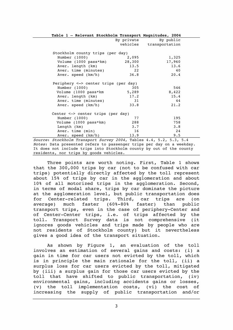
Table 1 – Relevant Stockholm Transport Magnitudes, 2004 By private By public
vehicles transportation Stockholm county trips (per day) Number (1000) 2,095 1,325 Volume (1000 pass*km) 28,300 17,960 Aver. length (km) 13.5 13.6 Aver. time (minutes) 22 40 Aver. speed (km/h) 36.8 20.4 Periphery <—> center trips (per day) Number (1000) 305 546 Volume (1000 pass*km 5,289 8,422 Aver. length (km) 17.2 15.4 Aver. time (minutes) 31 44 Aver. speed (km/h) 33.8 21.2 Center <—> center trips (per day) Number (1000) 77 195 Volume (1000 pass*km) 288 758 Length (km) 3.7 3.8 Aver. time (min) 16 24 Aver. speed (km/h) 13.9 9.5
Source: Stockholm Transport Survey 2004, Tables 4.4, 5.2, 5.3, 5.4 Notes: Data presented refers to passenger trips per day on a weekday. It does not include trips into Stockholm county by out of the county residents, nor trips by goods vehicles.
Three points are worth noting. First, Table 1 shows that the 300,000 trips by car (not to be confused with car trips) potentially directly affected by the toll represent about 15% of trips by car in the agglomeration and about 10% of all motorized trips in the agglomeration. Second, in terms of modal share, trips by car dominate the picture at the agglomeration level, but public transportation does for Center-related trips. Third, car trips are (on average) much faster (60%-80% faster) than public transport trips, even in the case of periphery-Center and of Center-Center trips, i.e. of trips affected by the toll. Transport Survey data is not comprehensive (it ignores goods vehicles and trips made by people who are not residents of Stockholm county) but it nevertheless gives a good idea of the transport situation.
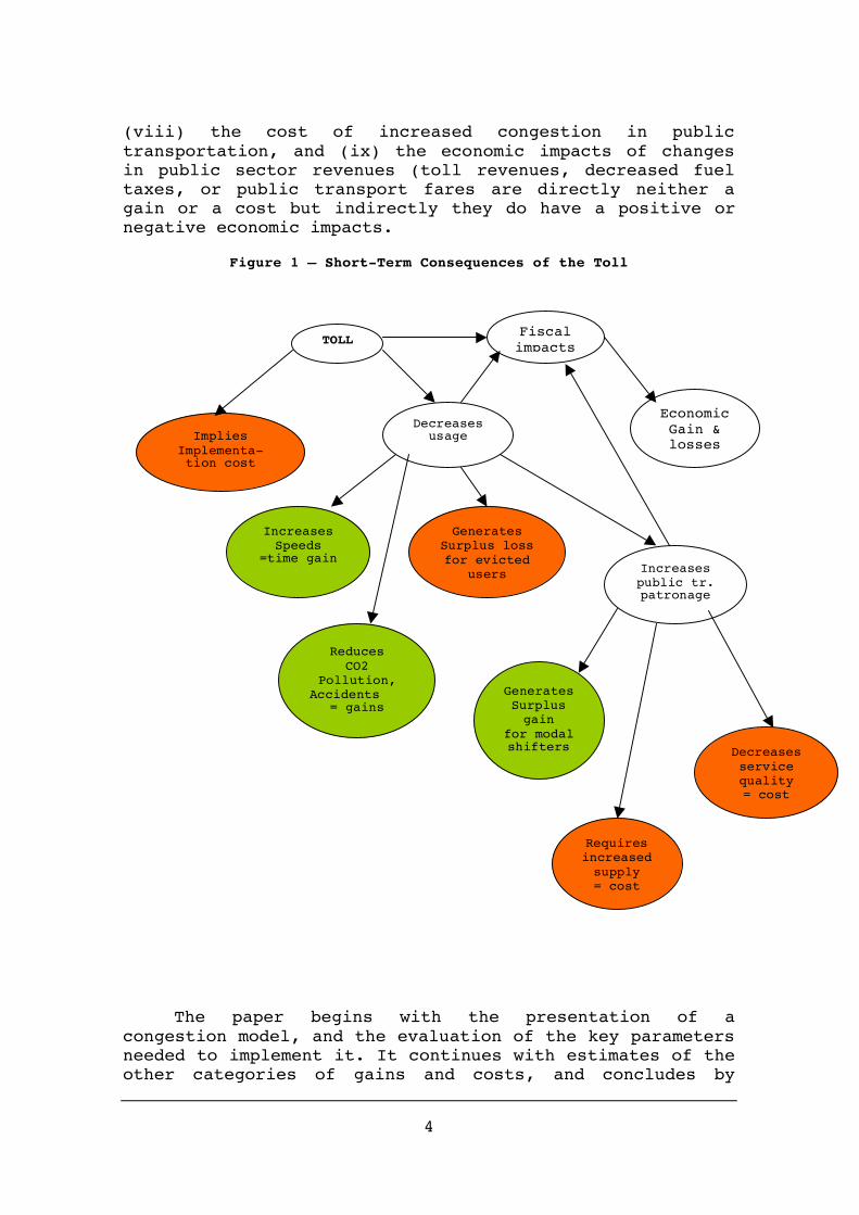
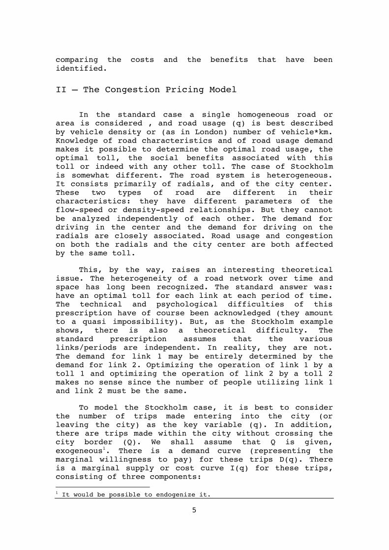
As shown by Figure 1, an evaluation of the toll involves an estimation of several gains and costs: (i) a gain in time for car users not evicted by the toll, which is in principle the main rationale for the toll, (ii) a surplus loss for car users evicted by the toll, mitigated by (iii) a surplus gain for those car users evicted by the toll that have shifted to public transportation, (iv) environmental gains, including accidents gains or losses, (v) the toll implementation costs, (vi) the cost of increasing the supply of public transportation and/or
4
(viii) the cost of increased congestion in public transportation, and (ix) the economic impacts of changes in public sector revenues (toll revenues, decreased fuel taxes, or public transport fares are directly neither a gain or a cost but indirectly they do have a positive or negative economic impacts.
Figure 1 – Short-Term Consequences of the Toll
The paper begins with the presentation of a congestion model, and the evaluation of the key parameters needed to implement it. It continues with estimates of the other categories of gains and costs, and concludes by
TOLL
Implies Implementa-tion cost
Decreases usage
Increases Speeds
=time gain
Reduces CO2
Pollution, Accidents
= gains
Generates Surplus loss for evicted
users Increases public tr. patronage
Generates Surplus gain
for modal shifters Decreases
service quality = cost
Requires increased supply = cost
Fiscal impacts
Economic Gain & losses
5
comparing the costs and the benefits that have been identified.
II – The Congestion Pricing Model
In the standard case a single homogeneous road or area is considered , and road usage (q) is best described by vehicle density or (as in London) number of vehicle*km. Knowledge of road characteristics and of road usage demand makes it possible to determine the optimal road usage, the optimal toll, the social benefits associated with this toll or indeed with any other toll. The case of Stockholm is somewhat different. The road system is heterogeneous. It consists primarily of radials, and of the city center. These two types of road are different in their characteristics: they have different parameters of the flow-speed or density-speed relationships. But they cannot be analyzed independently of each other. The demand for driving in the center and the demand for driving on the radials are closely associated. Road usage and congestion on both the radials and the city center are both affected by the same toll.
This, by the way, raises an interesting theoretical issue. The heterogeneity of a road network over time and space has long been recognized. The standard answer was: have an optimal toll for each link at each period of time. The technical and psychological difficulties of this prescription have of course been acknowledged (they amount to a quasi impossibility). But, as the Stockholm example shows, there is also a theoretical difficulty. The standard prescription assumes that the various links/periods are independent. In reality, they are not. The demand for link 1 may be entirely determined by the demand for link 2. Optimizing the operation of link 1 by a toll 1 and optimizing the operation of link 2 by a toll 2 makes no sense since the number of people utilizing link 1 and link 2 must be the same.
To model the Stockholm case, it is best to consider the number of trips made entering into the city (or leaving the city) as the key variable (q). In addition, there are trips made within the city without crossing the city border (Q). We shall assume that Q is given, exogeneous1. There is a demand curve (representing the marginal willingness to pay) for these trips D(q). There is a marginal supply or cost curve I(q) for these trips, consisting of three components: 1 It would be possible to endogenize it.
6
- a fixed cost C (fuel cost, depreciation, etc.); since this cost element is not affected by the toll it will be ignored in most of the analyses.
- a time cost cr(q) for the time spent on the radial. With τ the value of time, Sr the speed on the radial, w the average occupancy of cars and Lr the average length of radial trips affected by congestion, we have:
cr(q) = Lr*w*τ/Sr(q)
- a time cost cc(q) for the time spent in the center. With τ the value of time, Sc the speed on the radial, w the average occupancy of cars, and Lc the average length of trips in the center, we have:
cc(q) = Lc*w*τ/[Sc(q+Q)]
Hence:
I(q) = Lr*w*τ/Sr(q) + Lc*w*τ/[Sr(q+Q)]
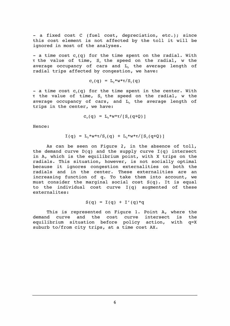
As can be seen on Figure 2, in the absence of toll, the demand curve D(q) and the supply curve I(q) intersect in A, which is the equilibrium point, with X trips on the radials. This situation, however, is not socially optimal because it ignores congestion externalities on both the radials and in the center. These externalities are an increasing function of q. To take them into account, we must consider the marginal social cost S(q). It is equal to the individual cost curve I(q) augmented of these externalites:
S(q) = I(q) + I’(q)*q
This is represented on Figure 1. Point A, where the demand curve and the cost curve intersect is the equilibrium situation before policy action, with q=X suburb to/from city trips, at a time cost AX.
7
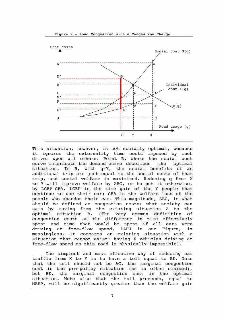
Figure 2 – Road Congestion with a Congestion Charge Unit costs Social cost S(q) N C M’ B’ M B Individual cost I(q) L H G A N’ B’’ P E F D(q) P’ E’ J H Road usage (q) Y’ Y X
This situation, however, is not socially optimal, because it ignores the externality time costs imposed by each driver upon all others. Point B, where the social cost curve intersects the demand curve describes the optimal situation. In B, with q=Y, the social benefits of an additional trip are just equal to the social costs of that trip, and social welfare is maximized. Reducing q from X to Y will improve welfare by ABC, or to put it otherwise, by LGEP-GBA. LGEP is the time gain of the Y people that continue to use their car; GBA is the welfare loss of the people who abandon their car. This magnitude, ABC, is what should be defined as congestion costs: what society can gain by moving from the existing situation A to the optimal situation B. (The very common definition of congestion costs as the difference in time effectively spent and time that would be spent if all cars were driving at free-flow speed, LAHJ in our Figure, is meaningless. It compares an existing situation with a situation that cannot exist: having X vehicles driving at free-flow speed on this road is physically impossible).
The simplest and most effective way of reducing car traffic from X to Y is to have a toll equal to BE. Note that the toll should not be AC, the marginal congestion cost in the pre-policy situation (as is often claimed), but BE, the marginal congestion cost in the optimal situation. Note also that the toll proceeds, equal to MBEP, will be significantly greater than the welfare gain
8
LGEP-GPA. To achieve a welfare gain of 100, a toll of 400 or more may be required.
The Stockholm toll certainly reduces road usage. But we cannot know before hand if it reduces it to the socially optimal level. The toll is likely to be lower or higher than the optimal toll. It will reduce road usage to Y’, with Y’ to the right or to the left of Y. In that case, the potential welfare gain will be reduced (by B’BB’’). Finding out whether the toll level is too high or too low (relative to the optimal toll) is one of the objective of the study.
For the analyst, the beauty of the Stockholm experiment is that it makes it possible to estimate the demand curve D(q). We know one point of this curve, point A, the equilibrium situation before the toll. We can know a second point of this curve, point B’, the equilibrium situation created by the toll. The quantity of trips entering the city after the toll, Y’, is recorded. The average toll can be deducted. It is added to the cost of the trip for q=Y’. Point B’ can therefore be determined. Having two points of D(q), it is easy to determine the equation of this demand curve.
Equipped with I(q), S(q) and D(q), we can easily calculate all the magnitudes we are interested in. We can determine point B, the socially optimum situation, with Y the socially optimal number of trips entering the city —what should be the policy goal. We can determine BE the optimal toll, and compare it with B’E’ the actual toll, and find out whether the present toll is too low or too high. We can also determine ABC-B’BB”” the social gain generated by the toll. This social gain is also equal to the time gained by non evicted car users, LHE’P’ minus the surplus loss of evicted car users HB’A.
III – Values of Key Parameters
To conduct the analysis, we need numbers on several key magnitudes that describe the Stockholm situation.
Number of trips q and Q
Trips into the city and out of the city q — We have data on the number of vehicles entering the city Center, and leaving the city Center, for “spring” 2005, and for May and April 2006, per day per periods of 15 minutes. This data is reported in Table 2.
9
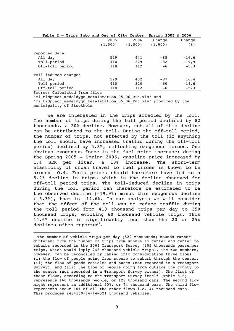
Table 2 – Trips Into and Out of City Center, Spring 2005 & 2006 2005 2006 Change Change (1,000) (1,000) (1,000) (%) Reported data: All day 529 441 -88 -16.6 Toll-period 410 329 -82 -19,9 Off-toll period 118 112 -6 -5.3 Toll induced changes All day 529 432 -87 16.4 Toll period 410 320 -60 -14.6 Off-toll period 118 112 -6 -5.3 Source: Calculated from files “mi_tidpunct_medeldygn_betalstation_05_06_Rin.xls” and “mi_tidpunct_medeldygn_betalstation_05_06_Rut.xls” produced by the municipality of Stockholm
We are interested in the trips affected by the toll. The number of trips during the toll period declined by 82 thousands, a 20% decline. However, not all of this decline can be attributed to the toll. During the off-toll period, the number of trips, not affected by the toll (if anything the toll should have increased traffic during the off-toll period) declined by 5.3%, reflecting exogenous forces. One obvious exogenous force is the fuel price increase: during the Spring 2005 – Spring 2006, gasoline price increased by 1.4 SEK per liter, a 13% increase. The short-term elasticity of urban travel to fuel prices is known to be around –O.4. Fuels prices should therefore have led to a 5.2% decline in trips, which is the decline observed for off-toll period trips. The toll-induced decline in trips during the toll period can therefore be estimated to be the observed decline (-19.9%) minus this exogenous decline (-5.3%), that is -14.6%. In our analysis we will consider that the effect of the toll was to reduce traffic during the toll period from 410 thousand trips per day to 350 thousand trips, evicting 60 thousand vehicle trips. This 14.6% decline is significantly less than the 20 or 25% declines often reported1. 1 The number of vehicle trips per day (529 thousands) sounds rather different from the number of trips from suburb to center and center to suburbs recorded in the 2004 Transport Survey (305 thousands passenger trips, which would imply 243 thousand vehicle trips). The two numbers, however, can be reconciled by taking into consideration three flows : (i) the flow of people going from suburb to suburb through the center, (ii) the flow of goods vehicles and buses (not recorded in a Transport Survey), and (iii) the flow of people going from outside the county to the center (not recorded in a Transport Survey either). The first of these flows, according to the Transport Survey itself (Table 5.6) represents 160 thousands people, or 128 thousand cars. The second flow might represent an additional 20%, or 74 thousand cars. The third flow represents about 10% of all the other flows i.e. 44 thousand cars. This produces 243+160+74+44=521 thousand vehicles.
10
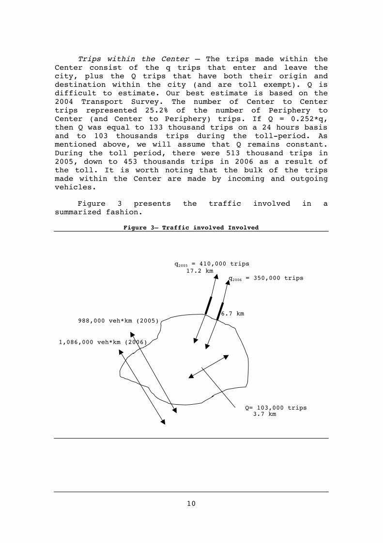
Trips within the Center — The trips made within the Center consist of the q trips that enter and leave the city, plus the Q trips that have both their origin and destination within the city (and are toll exempt). Q is difficult to estimate. Our best estimate is based on the 2004 Transport Survey. The number of Center to Center trips represented 25.2% of the number of Periphery to Center (and Center to Periphery) trips. If Q = 0.252*q, then Q was equal to 133 thousand trips on a 24 hours basis and to 103 thousands trips during the toll-period. As mentioned above, we will assume that Q remains constant. During the toll period, there were 513 thousand trips in 2005, down to 453 thousands trips in 2006 as a result of the toll. It is worth noting that the bulk of the trips made within the Center are made by incoming and outgoing vehicles.
Figure 3 presents the traffic involved in a summarized fashion.
Trips in the Center – The Transport Survey indicates the length of center to center car trips: 3.7 km. This is slightly longer than the 3.3 km radius of the charged zone. We will assume that 3.7 km is also the average length of trips made in the center by vehicles coming from outside the center.
Periphery-Center trips — It is more difficult to estimate the length of the part of radial trips affected by the charge, the part on which traffic declined and speed increased. According to the Transport Survey, the average length of periphery to center trips is 17 km. Substracting 3.7 km driven within the city, we are left with 13.3 km on radials. However, a substantial part of this mileage is done on non-congested arterial roads not affected by the toll, as a mere look at the maps showing changes in travel time by road sections will show. We will assume that 50% of these 13.3 km drive is affected by the toll, or 6.7 km. This is probably an overestimate1.
These estimates make it possible to produce Table 3 that shows the amount of traffic affected by the toll, in different ways. The q trips entering and leaving the Center are affected in terms of number and of speed, although the impact of the toll on speed is not the same on the radials and in the Center. The Q trips from Center to Center, that do not pay the toll, are affected in terms of speed.
1Data produced by a transport model suggests a shorter length. Traffic volumes (in vehicle*km) declined in the county by 435 thousand vehicles*km. Substracting the 266 thousand veh*km decline that took place in the charged zone, we are left with a decline of 169 thousand veh*km in the rest of the county. Most of that decline took place on the radials. Since traffic on these radials declined by 38 thousand vehicles, this would suggest an average length of about 4.4 km, or 2.2 km per trip. But this number is most probably an underestimate. The decline in traffic on the radials must have been compensated in part by increases in other parts of the country. The decline in traffic volume on the radials would therefore be greater, and so would the average length.
12
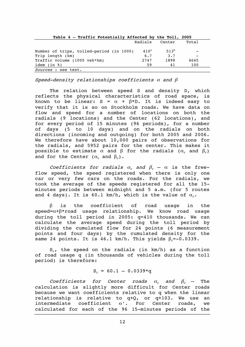
Table 4 – Traffic Potentially Affected by the Toll, 2005 Radials Center Total Number of trips, tolled-period (in 1000) 410a 513b - Trip length (km) 6.7 3.7 - Traffic volume (1000 veh*km) 2747 1898 4645 idem (in %) 59 41 100 Sources : see text.
Speed-density relationships coefficients α and β
The relation between speed S and density D, which reflects the physical characteristics of road space, is known to be linear: S = α + β*D. It is indeed easy to verify that it is so on Stockholm roads. We have data on flow and speed for a number of locations on both the radials (9 locations) and the Center (62 locations), and for every period of 15 minutes (96 periods), for a number of days (5 to 10 days) and on the radials on both directions (incoming and outgoing) for both 2005 and 2006. We therefore have about 10,000 pairs of observations for the radials, and 5952 pairs for the center. This makes it possible to estimate α and β for the radials (αr and βr) and for the Center (αc and βc).
Coefficients for radials αr and βr — α is the free-flow speed, the speed registered when there is only one car or very few cars on the roads. For the radials, we took the average of the speeds registered for all the 15-minutes periods between midnight and 5 a.m. (for 5 routes and 4 days). It is 60.1 km/h, which is the value of αr.
β is the coefficient of road usage in the speed=α+β*road usage relationship. We know road usage during the toll period in 2005: q=410 thousands. We can calculate the average speed during the toll period by dividing the cumulated flow for 24 points (6 measurement points and four days) by the cumulated density for the same 24 points. It is 46.1 km/h. This yields βr=-0.0339.
Sr, the speed on the radials (in km/h) as a function of road usage q (in thousands of vehicles during the toll period) is therefore:
Sr = 60.1 – 0.0339*q
Coefficients for Center roads αc and βc — The calculation is slightly more difficult for Center roads because we want coefficients relative to q when the linear relationship is relative to q+Q, or q+103. We use an intermediate coefficient α’. For Center roads, we calculated for each of the 96 15-minutes periods of the
13
day the average flow, average speed, and average density at 62 measurement points, then regressed speed as a function of density, then took the intercept of the regression. It is α’ and equal to 46.5 km/h.
The average speed on these roads is calculated as the cumulated flow during the toll period for our 62 points divided by the corresponding cumulated density. It is equal to 37.15 km/h. βc is extracted from 37.15=α’+βr*513. It is equal to -0.01823. Replacing 513 by q+103, we have 37.15=αc-0.01823*(q+103), which yields αc=43.3. Sc, speed in the Center as a function of road usage q (in thousands of vehicles during toll period) is therefore:
Sc = 43.3 – 0.01823*q
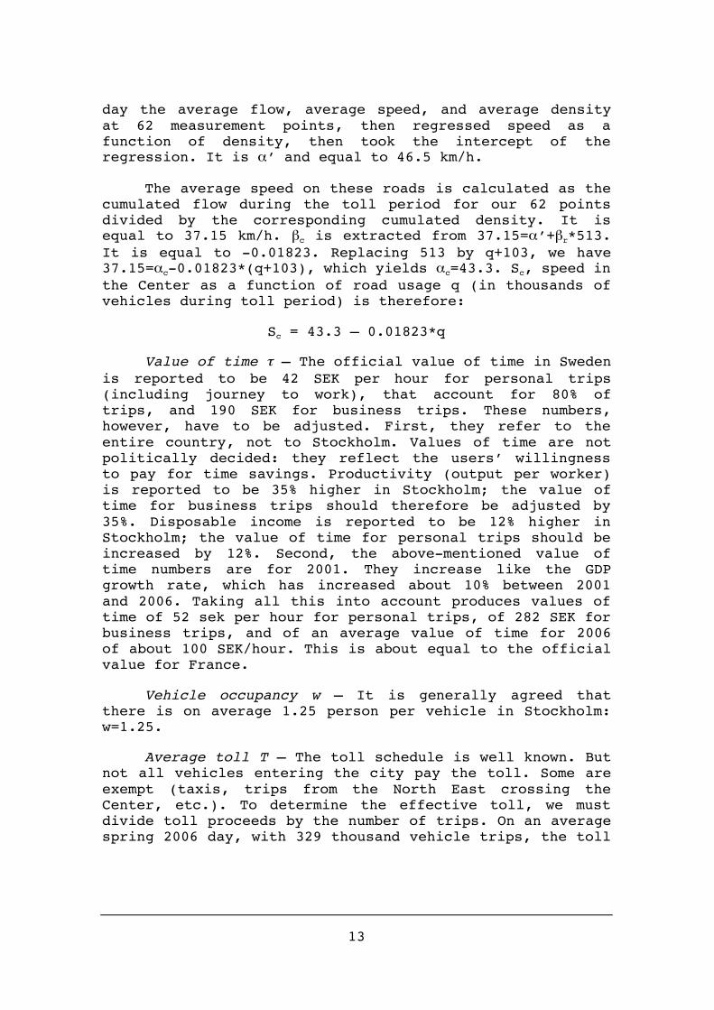
Value of time τ — The official value of time in Sweden is reported to be 42 SEK per hour for personal trips (including journey to work), that account for 80% of trips, and 190 SEK for business trips. These numbers, however, have to be adjusted. First, they refer to the entire country, not to Stockholm. Values of time are not politically decided: they reflect the users’ willingness to pay for time savings. Productivity (output per worker) is reported to be 35% higher in Stockholm; the value of time for business trips should therefore be adjusted by 35%. Disposable income is reported to be 12% higher in Stockholm; the value of time for personal trips should be increased by 12%. Second, the above-mentioned value of time numbers are for 2001. They increase like the GDP growth rate, which has increased about 10% between 2001 and 2006. Taking all this into account produces values of time of 52 sek per hour for personal trips, of 282 SEK for business trips, and of an average value of time for 2006 of about 100 SEK/hour. This is about equal to the official value for France.
Vehicle occupancy w – It is generally agreed that there is on average 1.25 person per vehicle in Stockholm: w=1.25.
Average toll T – The toll schedule is well known. But not all vehicles entering the city pay the toll. Some are exempt (taxis, trips from the North East crossing the Center, etc.). To determine the effective toll, we must divide toll proceeds by the number of trips. On an average spring 2006 day, with 329 thousand vehicle trips, the toll
14
proceeds were 3.18 M SEK/day. This amounts to 9.7 SEK per trip on average1.
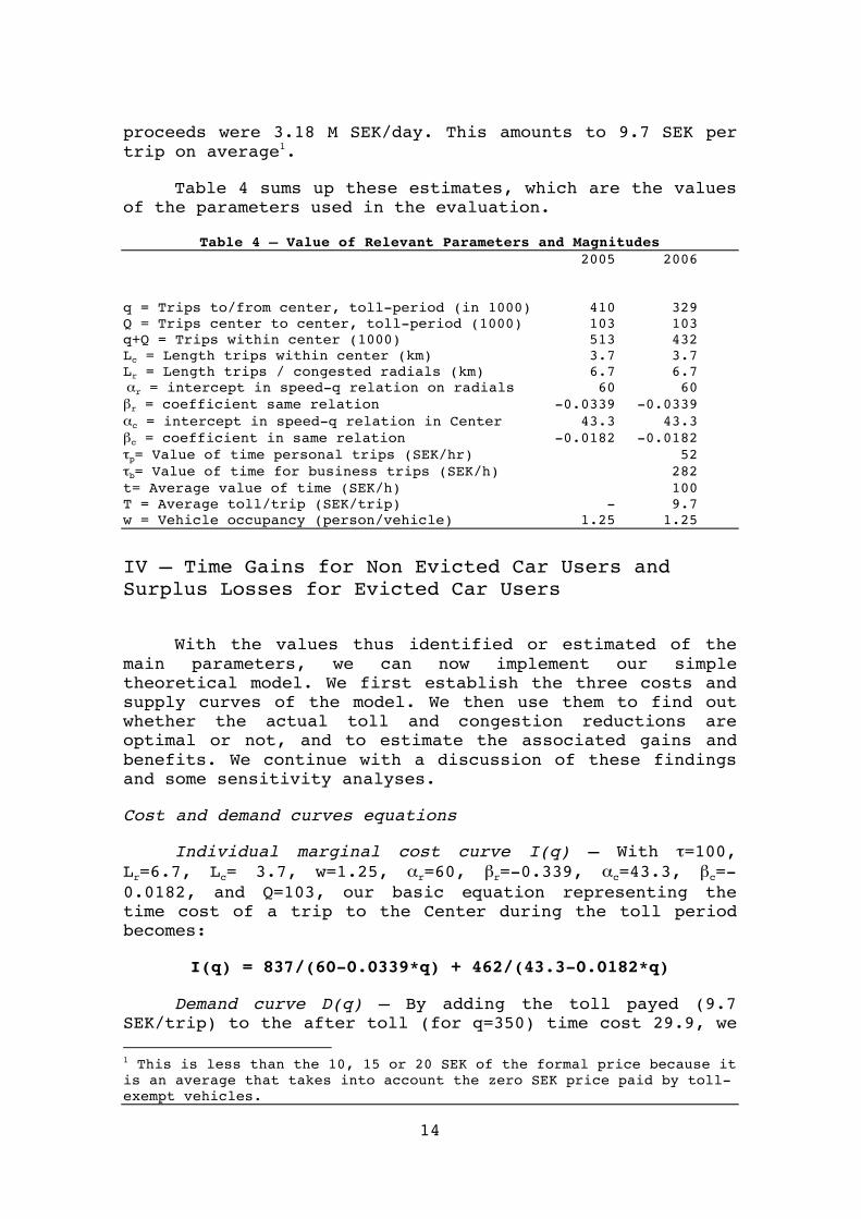
Table 4 sums up these estimates, which are the values of the parameters used in the evaluation.
Table 4 – Value of Relevant Parameters and Magnitudes 2005 2006 q = Trips to/from center, toll-period (in 1000) 410 329 Q = Trips center to center, toll-period (1000) 103 103 q+Q = Trips within center (1000) 513 432 Lc = Length trips within center (km) 3.7 3.7 Lr = Length trips / congested radials (km) 6.7 6.7 αr = intercept in speed-q relation on radials 60 60 βr = coefficient same relation -0.0339 -0.0339 αc = intercept in speed-q relation in Center 43.3 43.3 βc = coefficient in same relation -0.0182 -0.0182 τp= Value of time personal trips (SEK/hr) 52 τb= Value of time for business trips (SEK/h) 282 t= Average value of time (SEK/h) 100 T = Average toll/trip (SEK/trip) - 9.7 w = Vehicle occupancy (person/vehicle) 1.25 1.25
IV – Time Gains for Non Evicted Car Users and Surplus Losses for Evicted Car Users
With the values thus identified or estimated of the main parameters, we can now implement our simple theoretical model. We first establish the three costs and supply curves of the model. We then use them to find out whether the actual toll and congestion reductions are optimal or not, and to estimate the associated gains and benefits. We continue with a discussion of these findings and some sensitivity analyses.
Cost and demand curves equations
Individual marginal cost curve I(q) — With τ=100, Lr=6.7, Lc= 3.7, w=1.25, αr=60, βr=-0.339, αc=43.3, βc=-0.0182, and Q=103, our basic equation representing the time cost of a trip to the Center during the toll period becomes:
I(q) = 837/(60-0.0339*q) + 462/(43.3-0.0182*q)
Demand curve D(q) — By adding the toll payed (9.7 SEK/trip) to the after toll (for q=350) time cost 29.9, we 1 This is less than the 10, 15 or 20 SEK of the formal price because it is an average that takes into account the zero SEK price paid by toll-exempt vehicles.
15
obtain the price paid by users after toll: 39.6 SEK per trip. This defines the coordinates of point B’ (350, 39.6). We already have the coordinates of point A (410, 31.8). Points A and B’ are two points of the demand curve. Its equation is:
D(q) = 89.51 – 0.1425*q
Social cost curve S(q) — The social cost curve S(q) is equal to the individual cost curve plus the derivative of this individual cost curve multiplied by the number of trips. Note that for the part of the equation that measures social cost in the Center, the relevant « number of trips » (that multiples the derivative) is not q, but q+Q. An additional trip to the Center slows down not only the q vehicles driving to/from the Center, but also the Q vehicles driving from the Center to the Center. The resulting equation of S(q) is a bit long, but can easily be handled with a spread sheet :
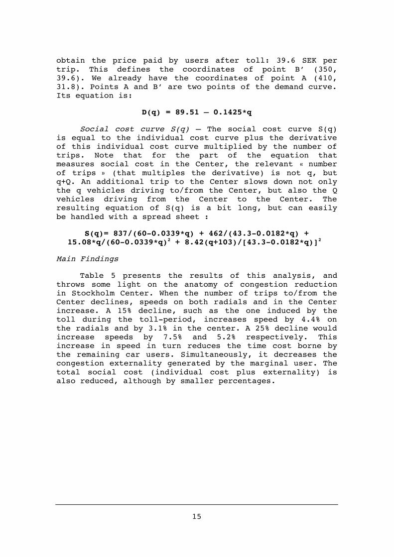
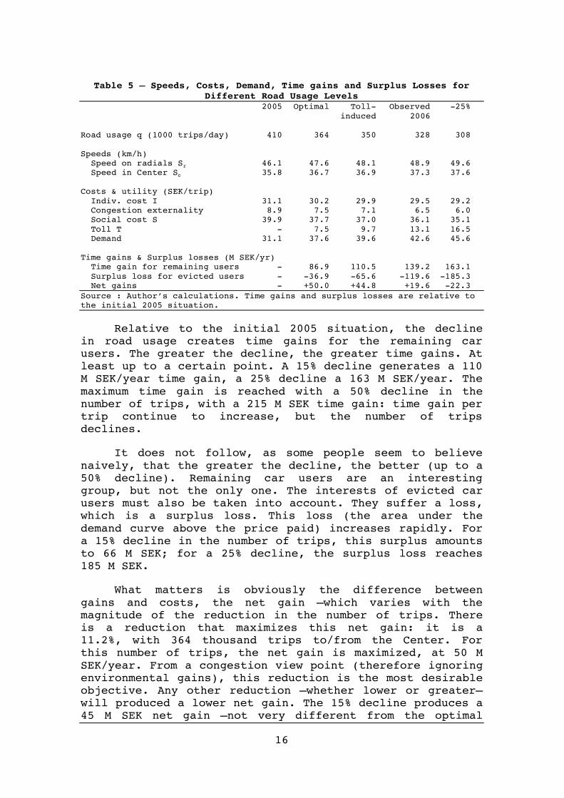
Table 5 presents the results of this analysis, and throws some light on the anatomy of congestion reduction in Stockholm Center. When the number of trips to/from the Center declines, speeds on both radials and in the Center increase. A 15% decline, such as the one induced by the toll during the toll-period, increases speed by 4.4% on the radials and by 3.1% in the center. A 25% decline would increase speeds by 7.5% and 5.2% respectively. This increase in speed in turn reduces the time cost borne by the remaining car users. Simultaneously, it decreases the congestion externality generated by the marginal user. The total social cost (individual cost plus externality) is also reduced, although by smaller percentages.
16
Table 5 – Speeds, Costs, Demand, Time gains and Surplus Losses for Different Road Usage Levels
2005 Optimal Toll- Observed -25% induced 2006 Road usage q (1000 trips/day) 410 364 350 328 308 Speeds (km/h) Speed on radials Sr 46.1 47.6 48.1 48.9 49.6 Speed in Center Sc 35.8 36.7 36.9 37.3 37.6 Costs & utility (SEK/trip) Indiv. cost I 31.1 30.2 29.9 29.5 29.2 Congestion externality 8.9 7.5 7.1 6.5 6.0 Social cost S 39.9 37.7 37.0 36.1 35.1 Toll T - 7.5 9.7 13.1 16.5 Demand 31.1 37.6 39.6 42.6 45.6 Time gains & Surplus losses (M SEK/yr) Time gain for remaining users - 86.9 110.5 139.2 163.1 Surplus loss for evicted users - -36.9 -65.6 -119.6 -185.3 Net gains - +50.0 +44.8 +19.6 -22.3 Source : Author’s calculations. Time gains and surplus losses are relative to the initial 2005 situation.
Relative to the initial 2005 situation, the decline in road usage creates time gains for the remaining car users. The greater the decline, the greater time gains. At least up to a certain point. A 15% decline generates a 110 M SEK/year time gain, a 25% decline a 163 M SEK/year. The maximum time gain is reached with a 50% decline in the number of trips, with a 215 M SEK time gain: time gain per trip continue to increase, but the number of trips declines.
It does not follow, as some people seem to believe naively, that the greater the decline, the better (up to a 50% decline). Remaining car users are an interesting group, but not the only one. The interests of evicted car users must also be taken into account. They suffer a loss, which is a surplus loss. This loss (the area under the demand curve above the price paid) increases rapidly. For a 15% decline in the number of trips, this surplus amounts to 66 M SEK; for a 25% decline, the surplus loss reaches 185 M SEK.
What matters is obviously the difference between gains and costs, the net gain —which varies with the magnitude of the reduction in the number of trips. There is a reduction that maximizes this net gain: it is a 11.2%, with 364 thousand trips to/from the Center. For this number of trips, the net gain is maximized, at 50 M SEK/year. From a congestion view point (therefore ignoring environmental gains), this reduction is the most desirable objective. Any other reduction —whether lower or greater— will produced a lower net gain. The 15% decline produces a 45 M SEK net gain —not very different from the optimal
17
decline. A 20% decline, to 329 thousands trips, produces a 20 M SEK net gain. A 25% decline, to 308 thousands trips, even produces a net loss of 22 M SEK: the surplus loss for evicted car users is then greater than the time gain for remaining car users.
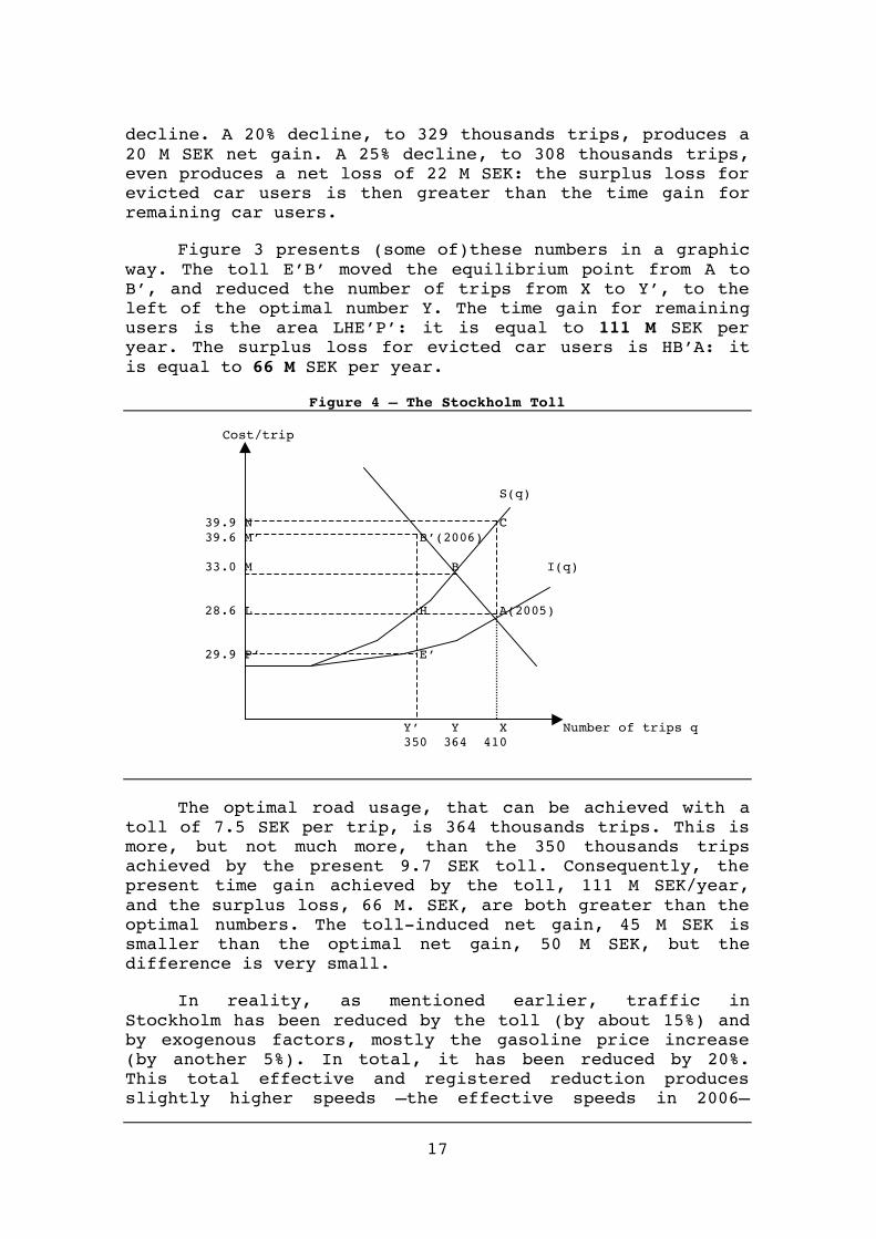
Figure 3 presents (some of)these numbers in a graphic way. The toll E’B’ moved the equilibrium point from A to B’, and reduced the number of trips from X to Y’, to the left of the optimal number Y. The time gain for remaining users is the area LHE’P’: it is equal to 111 M SEK per year. The surplus loss for evicted car users is HB’A: it is equal to 66 M SEK per year.
Figure 4 – The Stockholm Toll Cost/trip S(q) 39.9 N C 39.6 M’ B’(2006) 33.0 M B I(q) 28.6 L H A(2005) 29.9 P’ E’ Y’ Y X Number of trips q 350 364 410
The optimal road usage, that can be achieved with a toll of 7.5 SEK per trip, is 364 thousands trips. This is more, but not much more, than the 350 thousands trips achieved by the present 9.7 SEK toll. Consequently, the present time gain achieved by the toll, 111 M SEK/year, and the surplus loss, 66 M. SEK, are both greater than the optimal numbers. The toll-induced net gain, 45 M SEK is smaller than the optimal net gain, 50 M SEK, but the difference is very small.
In reality, as mentioned earlier, traffic in Stockholm has been reduced by the toll (by about 15%) and by exogenous factors, mostly the gasoline price increase (by another 5%). In total, it has been reduced by 20%. This total effective and registered reduction produces slightly higher speeds —the effective speeds in 2006—
18
higher time gains (139 M SEK) but also higher surplus loss (120 M SEK) and in the end a lower net gain of about 20 M SEK per year.
This analysis refers to the main impact of the toll upon traffic congestion. To be complete two additional impacts must be discussed, and estimated.
Time Loss Associated to Traffic Diversion to the Essingeleden and Södra Länken Highway.
To avoid the toll, some of the vehicles that were entering the Center in 2005 are now by passing the Center and using the non-tolled Essingeleden and Södra Länken bypass, thereby increasing traffic and lowering speeds (relative to what would have happened in the absence of toll) and causing time losses. This appears very clearly on the maps depicting changes in travel time presented in Stocholmsforöket 2006 (p. 7).
Between 2005 and 2006, traffic did increase on the ring road. This increase varies from one section of the road to another. The best estimate available, in terms of vehicle-km, puts this increase at 9.9%, from 988,000 to 1086,000. In a context of declining road traffic in the entire county, it is reasonable to assume that this increase consists of traffic discouraged by the toll. One could even think that the toll-induced traffic is more important because of the exogenous (fuel price increases) decline in road traffic in the county. To be on the safe side, we will retain this 9.9% increase.
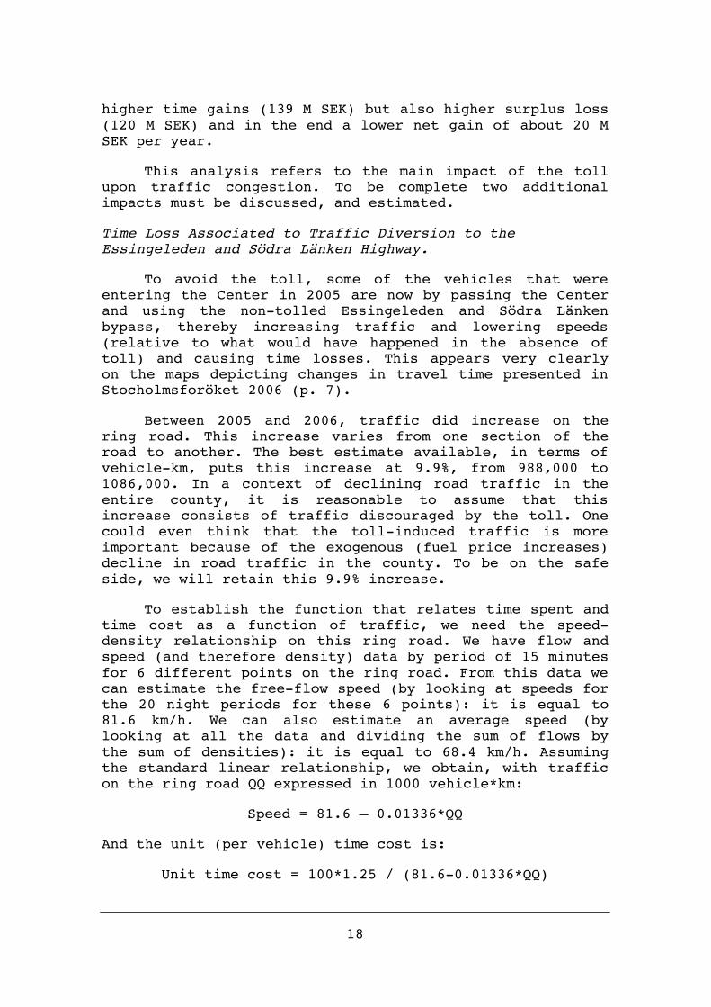
To establish the function that relates time spent and time cost as a function of traffic, we need the speed-density relationship on this ring road. We have flow and speed (and therefore density) data by period of 15 minutes for 6 different points on the ring road. From this data we can estimate the free-flow speed (by looking at speeds for the 20 night periods for these 6 points): it is equal to 81.6 km/h. We can also estimate an average speed (by looking at all the data and dividing the sum of flows by the sum of densities): it is equal to 68.4 km/h. Assuming the standard linear relationship, we obtain, with traffic on the ring road QQ expressed in 1000 vehicle*km:
Speed = 81.6 – 0.01336*QQ
And the unit (per vehicle) time cost is:
Unit time cost = 100*1.25 / (81.6-0.01336*QQ)
19
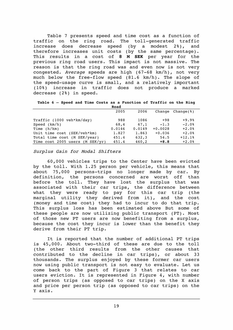
Table 7 presents speed and time cost as a function of traffic on the ring road. The toll-generated traffic increase does decrease speed (by a modest 2%), and therefore increases unit costs (by the same percentage). This results in a cost of 8 M SEK per year for the previous ring road users. This impact is not massive. The reason is that the ring road was and even now is not very congested. Average speeds are high (67-68 km/h), not very much below the free-flow speed (81.6 km/h). The slope of the speed-usage curve is small, and a relatively important (10%) increase in traffic does not produce a marked decrease (2%) in speed.
Table 6 – Speed and Time Costs as a Function of Traffic on the Ring Road
2005 2006 Change Change(%) Traffic (1000 veh*km/day) 988 1086 +98 +9.9% Speed (km/h) 68,4 67,1 -1.3 -2.0% Time (h/km) 0.0146 0.0149 +0.0028 +2.0% Unit time cost (SEK/veh*km) 1.827 1.863 +0.036 +2.0% Total time cost (M SEK/year) 451.4 632,3 54.5 +12.1% Time cost 2005 users (M SEK/yr) 451.4 460,2 +8.8 +2.0%
Surplus Gain for Modal Shifters
60,000 vehicles trips to the Center have been evicted by the toll. With 1.25 person per vehicle, this means that about 75,000 persons-trips no longer made by car. By definition, the persons concerned are worst off than before the toll. They have lost the surplus that was associated with their car trips, the difference between what they were ready to pay for this car trip (the marginal utility they derived from it), and the cost (money and time cost) they had to incur to do that trip. This surplus loss has been estimated above But some of these people are now utilizing public transport (PT). Most of those new PT users are now benefiting from a surplus, because the cost they incur is lower than the benefit they derive from their PT trip.
It is reported that the number of additional PT trips is 45,000. About two-third of these are due to the toll (the other third results from the other causes that contributed to the decline in car trips), or about 33 thousands. The surplus enjoyed by these former car users now using public transport is not easy to evaluate. Let us come back to the part of Figure 3 that relates to car users eviction. It is represented in Figure 4, with number of person trips (as opposed to car trips) on the X axis and price per person trip (as opposed to car trips) on the Y axis.
20
Figure 5 – Gains and Losses for Evicted Car Users Price per person trip 31.7 N’ B’ 28.7 I K 24.9 L H J A Y’ Z X Person trips (q°) 438 471 513
The number of person-trips by car has been reduced by 75 thousands as a result of an increase in price of 6.8 SEK per trip. Let us assume that the people who shifted to public transportation are those who enjoyed the greatest car transportation surplus (amongst evicted people), because the marginal utility of their trips was greatest. They are the Y’Z people (or rather trips) on Figure 3. We can look at the B’A curve as the demand curve for public transport of evicted people. HJ (or Y’Z) persons pay a HI price for public transport. They enjoy a IB’K surplus. This surplus amounts to 12.4 M SEK per year.
Discussion
The time loss on the ring road (-12 M SEK) and the surplus gain of modal shifters (+12 M SEK) do not add much to the timegains (+111 M SEK) and welfare losses (-66) of the core analysis. How robust are these numbers? A sensitivity analysis and a consistency check with the implied demand elasticity provide partial answers.
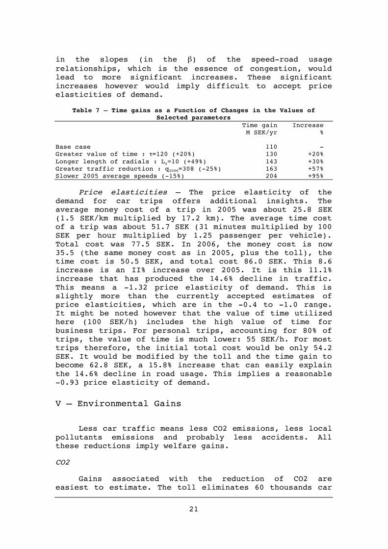
Sensitivity analysis – For some of the parameters of the model, the values utilized, as they appear in Table 4, are at times somewhat questionable. We calculated the sensitivity of the model to changes in these values, limiting ourselves to changes that would increase the value of the time gains. The results of this exercise are presented in Table n. They are rather reassuring. A higher value of time, or a longer length of the radials affected by improve speed, or a greater reduction of traffic into/out of the Center would indeed increase the time gains. But they would do so in modest proportions. Changes
21
in the slopes (in the β) of the speed-road usage relationships, which is the essence of congestion, would lead to more significant increases. These significant increases however would imply difficult to accept price elasticities of demand.
Table 7 – Time gains as a Function of Changes in the Values of Selected parameters
Time gain Increase M SEK/yr % Base case 110 - Greater value of time : τ=120 (+20%) 130 +20% Longer length of radials : Lr=10 (+49%) 143 +30% Greater traffic reduction : q2006=308 (-25%) 163 +57% Slower 2005 average speeds (-15%) 204 +95%
Price elasticities – The price elasticity of the demand for car trips offers additional insights. The average money cost of a trip in 2005 was about 25.8 SEK (1.5 SEK/km multiplied by 17.2 km). The average time cost of a trip was about 51.7 SEK (31 minutes multiplied by 100 SEK per hour multiplied by 1.25 passenger per vehicle). Total cost was 77.5 SEK. In 2006, the money cost is now 35.5 (the same money cost as in 2005, plus the toll), the time cost is 50.5 SEK, and total cost 86.0 SEK. This 8.6 increase is an II% increase over 2005. It is this 11.1% increase that has produced the 14.6% decline in traffic. This means a -1.32 price elasticity of demand. This is slightly more than the currently accepted estimates of price elasticities, which are in the -0.4 to -1.0 range. It might be noted however that the value of time utilized here (100 SEK/h) includes the high value of time for business trips. For personal trips, accounting for 80% of trips, the value of time is much lower: 55 SEK/h. For most trips therefore, the initial total cost would be only 54.2 SEK. It would be modified by the toll and the time gain to become 62.8 SEK, a 15.8% increase that can easily explain the 14.6% decline in road usage. This implies a reasonable -0.93 price elasticity of demand.
V – Environmental Gains
Less car traffic means less CO2 emissions, less local pollutants emissions and probably less accidents. All these reductions imply welfare gains.
CO2
Gains associated with the reduction of CO2 are easiest to estimate. The toll eliminates 60 thousands car
22
trips of 17.2 km (See Table 1) between the periphery and the Center. It saves 1.03 M vehicle*km/day. This is a serious overevaluation because it assumes that the toll did not induce more or longer trips in the rest of the agglomeration. Assuming an average consumption of 0.1 liters per km, and knowing that 1 liter of fuel consumed produces 2.35 kg of CO2, the toll led to a reduction of 300,000 kg, or 342 tons of CO2. There is a European market on which CO2 emissions rights are exchanged at a price. The present market price (see www.point.carbon.com) is 16.6 €, or 166 SEK per ton. The value of CO2 reductions is 10 M SEK per year1.
Air pollution
Gains associated with the reduction of local pollutants (NOx, particulates, etc.) are more difficult to estimate. Emissions were reduced like traffic: by about 15%. Air pollution costs were reduced by about this percentage. But we have no estimate of air pollution costs in 2005. We shall use the French official value that estimates the marginal cost of local air pollution created by one vehicle*km driven in “dense urban area”2 at 0.029 € or 0.29 SEK. The toll induced reduction of 1.03 M vehicle*km is therefore associated with a gain of 74.7 M SEK per year3.
Accidents
The impact of the toll on accidents is twofold. On the one hand, there are less vehicle*km driven, and therefore a lower probability of accidents. This factor would account for a 15% reduction in accidents.
On the other hand, these vehicles are driven at higher speeds, which increases the probability and seriousness of accidents per vehicle*km. The relationship usually accepted (which is based on a Swedish study) is the following. With s1 and s2 the speed in 1 and 2, the number of accidents is multiplied by (s2/s1)λ with λ=2 for accidents, λ=3 for serious accidents and λ=4 for 1 The Evaluation report (Stockholmsforsöket 2006 p. 119) values reductions in CO2 emissions at 64 M SEK/year. This is probably because it uses a value of the ton of CO2 much higher than the one presently found on the market. 2 Ministère de l’Equipement, Instruction-cadre relative aux méthodes d’évaluation économique des grands projets d’infrastructures de transport, 25.3.2004, Annex I p. 5. Dense urban area is defined as an area with a density higher than 420 inhabitants/km2. The density of the Stockholm « metropolitan area » is 498 inh./km2. 3 The Evaluation report (Stockholmsforsöket 2006 p. 119) values reductions in air pollution emissions at 22 M SEK/year.
23
fatalities. The changes in speed arrived at in this study imply for the part of trips on the radials increases of 9% for accidents at large, of 14% for serious accidents and of 19% for fatalities; for the part of trips in the Center, the increases are respectively 6%, 9% and 13%. On average this is about 8% for accidents, 12% for serious accidents and 17% for fatalities. Note that greater increases in speed would produce much higher increases in accident rates.
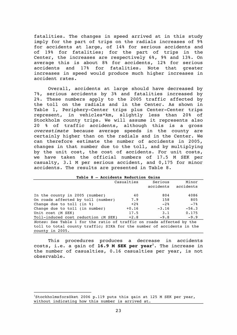
Overall, accidents at large should have decreased by 7%, serious accidents by 3% and fatalities increased by 2%. These numbers apply to the 2005 traffic affected by the toll on the radials and in the Center. As shown in Table 1, Periphery-Center trips plus Center-Center trips represent, in vehicles*km, slightly less than 20% of Stockholm county trips. We will assume it represents also 20 % of traffic accidents, although this is a gross overestimate because average speeds in the county are certainly higher than on the radials and in the Center. We can therefore estimate the number of accidents in 2005, changes in that number due to the toll, and by multiplying by the unit cost, the cost of accidents. For unit costs, we have taken the official numbers of 17.5 M SEK per casualty, 3.1 M per serious accident, and 0,175 for minor accidents. The results are presented in Table 8.
Table 8 – Accidents Reduction Gains Casualties Serious Minor accidents accidents In the county in 2005 (number) 40 804 4086 On roads affected by toll (number) 7.9 158 805 Change due to toll (in %) +2% -2% -7% Change due to toll (in number) +0.16 -3.16 -56.3 Unit cost (M SEK) 17.5 3.1 0.175 Toll-induced cost reduction (M SEK) +2.8 -9.8 -9.9 Notes: See Table 1 for the ratio of traffic on roads affected by the toll to total county traffic; SIKA for the number of accidents in the county in 2005.
This procedures produces a decrease in accidents costs, i.e. a gain of 16.9 M SEK per year1. The increase in the number of casualties, 0.16 casualties per year, is not observable.
1Stockholmsforsöket 2006 p.119 puts this gain at 125 M SEK per year, without indicating how this number is arrived at.
24
VI – Toll Implementation Costs
The cost of the toll should in principle be easy to determine because the toll conception, development and implementation has been contracted out by the National Road Administration to IBM, a private company. Only a few elements of the cost have been paid directly by the National Road Administration (some infrastructure investments for 94 M SEK, prosecution costs for 15 M SEK, tax administration expenditures for 24 M SEK) or by the municipality of Stockholm (information costs for 80 M SEK). There are several difficulties, however. The contract with IBM, for 1880 M SEK was for the seven months period of the trial. It included initial investments and operation costs for that period. It appears that operation costs, presently estimated at about 25 M SEK per month, are declining regularly; operation costs of the first months included software developments that could and should be considered as investments. “Regular” operation costs —what it would cost to run the system on a regular basis— are not known, but are certainly lower. They are officially estimated to be 17.5 M SEK per month. This estimate, which would be used by the National Road Administration in renegotiating a contract with IBM, may well be on the low side. Let us assume a regular operation cost of 20 M SEK per month. The difference between the amount paid to IBM and seven times this monthly operation cost can be assumed to be the investment made by IBM. It is equal to 1880-7*20 = 1740 M SEK. To this amount should be added the toll-related additional road expenditure of 94 M SEK.
Investment cost = IBM contract – regular operation costs for 7 months + additional investments
The cost of the Stockholm toll must therefore be estimated on the basis of an investment of 1830 M SEK1 and of a yearly operation cost of 240 M SEK (12*20). The yearly cost, the one that is of interest to us, consists of operation costs, plus amortization of the capital invested, plus the opportunity cost of this capital, plus the marginal cost of the public funds invested.
Amortization - Over what period should this investment be amortized? It consists of hardware 1 This may be an underestimate. Some reports put additional charge system costs for the Road Administration (including the investments taken into account here) at 300 MSEK, for the Municipality of Stockholm at 300 MSEK, and for Q-Free the enterprise that provides transponders at 140 MSEK.
25
(transponders, cameras, lasers, computers, gantries) that has a relatively short life, and of software (computer programmes, design, knowledge, system manuals) that has also a relatively short life. Five to seven years might be a good bet. Let us assume 6 years.
Opportunity cost of capital - The opportunity cost of capital —the fact that the public funds invested in the toll would have produced utility had they been invested in other areas, such as research for instance— must be at least 5%.
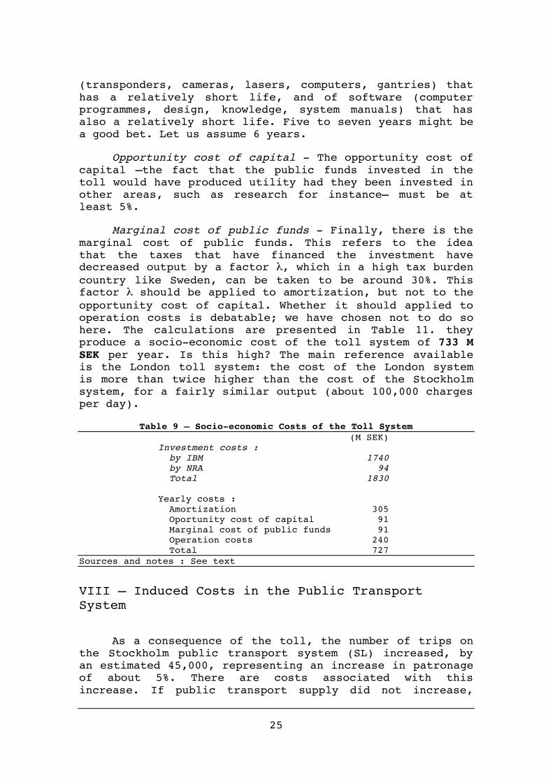
Marginal cost of public funds - Finally, there is the marginal cost of public funds. This refers to the idea that the taxes that have financed the investment have decreased output by a factor λ, which in a high tax burden country like Sweden, can be taken to be around 30%. This factor λ should be applied to amortization, but not to the opportunity cost of capital. Whether it should applied to operation costs is debatable; we have chosen not to do so here. The calculations are presented in Table 11. they produce a socio-economic cost of the toll system of 733 M SEK per year. Is this high? The main reference available is the London toll system: the cost of the London system is more than twice higher than the cost of the Stockholm system, for a fairly similar output (about 100,000 charges per day).
Table 9 – Socio-economic Costs of the Toll System (M SEK) Investment costs : by IBM 1740 by NRA 94 Total 1830 Yearly costs : Amortization 305 Oportunity cost of capital 91 Marginal cost of public funds 91 Operation costs 240 Total 727 Sources and notes : See text
VIII – Induced Costs in the Public Transport System
As a consequence of the toll, the number of trips on the Stockholm public transport system (SL) increased, by an estimated 45,000, representing an increase in patronage of about 5%. There are costs associated with this increase. If public transport supply did not increase,
26
public transport congestion increased: the ratio of demand to supply, an indicator of public transport quality, deteriorated, inflicting a cost upon the many public transport users. If public transport supply increased, this was done at a cost. It seems that both phenomena took place in Stockholm.
Cost of increase in public transport supply
It is very difficult to increase public transport supply in Stockholm, for technical and economic reason. The only significant increase introduced in conjunction with the toll was the purchase of about 200 buses put on service on 16 suburban lines at peak hours. This introduction took place in August 2005. It is reported that the associated investment amounts to 580 M SEK, and that associated yearly operation costs amount to 341 M SEK. Table 10 presents these costs on a yearly basis. The cost of increased bus supply is estimated at 508 M SEK per year.
Table 10 – Socio Economic Costs of Increased Public Transport Supply M SEK Investment costs 580 Yearly costs: Amortizationa 106 Opportunity cost of capital 29 Marginal cost of public fund 32 Operation costs 341 Total 508 Notes: aover 5 years. b5% if investment cost. c30% of amortization costs
Cost of increased congestion in public transport
In spite of this increase in public transport supply, it appears that travel conditions in public transport deteriorated somewhat. Punctuality declined by about 5% in the subway and in commuter rail services (Stockholmsfosöket 2006 p. 51). Cancellations of scheduled subway and commuter trains increased. The proportion of standing passengers increased in the underground (+2 percentage points), in suburban trains (+2 percentage points), in inner city bus services (+ 1 percentage point) but decreased (-1 percentage point) in commuter trains (ibidem). Public transport ability to keep on time was also poorer in Spring 2006 than in Spring 2005.Overall, the proportion of public transport passengers who are satisfied decreased from 66% in Spring 2005 to 61% in Spring 2006 (ibidem).
27
We cannot be sure that this decrease in quality level is the result of the increased public transport patronage brought about by the toll. However, it is obvious that there must a causal link between more people and less quality. This link is the form taken by congestion in public transportation. With scheduled trips, additional patronage results in lower service quality, or to put it otherwise, in higher non monetary costs.
It is difficult to put a money value on these costs. We can nevertheless offer the following estimate. For SL, the Stockholm public transport company, if the value of time of people seated in public transport is 1, the value of time of people standing in buses is 2, the value of time of people standing in railways in moderate congestion is 1.5 and in severe congestion is 2. According to the Transport Survey, the average duration of public transport trips is 40 minutes. Assuming that one fourth of this time is access and waiting time, time spent in public transport is on average 30 minutes. The total amount of time spent in public transportation is about 662,000 h per day (1,325 thousands trips of 30 minutes each). A 1.34 percentage point increase1 in the number of standing travelers represents 8,900 hours of additional standing per day. Valued at 100 SEK per hour, this amounts to 222 M SEK per year. This is a fragile estimate, but it gives an order of magnitude of the welfare loss caused by increased congestion in public transportation.
VIII — Economic Impacts of Changes in Public Revenues
Toll proceeds – In principle, and contrary to what some commentators believe, the money raised as toll payment, which amounts to 792 M SEK per year, should be ignored. This amount is neither a gain nor a cost. It is a transfer. It is money taken out of the pocket of car users, which obviously decreases their welfare, and welfare in general. But it is money that increases the revenues of public bodies, and that will supposedly be spent usefully (for transportation purposes or not, it does not really matters) and will therefore increase welfare by the same amount. The two welfare changes cancel each other. It would be a mistake to count as a benefit the useful actions that will be financed by this payment, while ignoring the cost borne by those who pay the toll. 1 This is the average of changes in the various public transport means (underground, buses, etx.) weighted by the importance of « boardings » on each of these means.
28
It would equally be a mistake to count as a cost the toll paid by car users while ignoring the welfare benefits the toll payments will finance. Both must be counted, or more simply, ignored.
However, it can be argued that this money, which accrues to the national Treasury, is much less distortionary than ordinary taxes. As a matter of fact, it is not distortionary at all, since it modifies behaviors in a desirable direction. It is therefore justified to apply the marginal cost of public funds to toll proceeds, and to count 234 M SEK (792x30%) as a social benefit.
Fuel taxes — A similar issue arises with respect to the reduction in fuels taxes brought by the toll. We estimated the fuel consumption reduction to be 103 M liters per year. With taxes of about 7 SEK per liter, this is a tax loss of 70 M SEK per year for the Treasury. Fuels taxes are not distortionary, and they are likely to be replaced by more distortionary taxes. We can therefore apply the marginal cost of public funds to this amount and count 21 M SEK per year as a social cost.
Public transport fares – Public transport users pay about half operation costs, and this applies also to the additional passengers generated by the toll, for about 170 M SEK per year. It has been argued that these fares decrease the need for public subsidies and the marginal cost of public funds that come with them, and that 30% of these 170 M. SEK should be counted as a social benefit. This would be true if we had added a marginal cost of public funds to the operation costs. But since we did not do so, there is no reason to count the marginal cost of public funds as a benefit.
IX - Costs and Gains Compared
Table n summarize our findings. It shows that costs outweight benefits by more than one billion SEK per year. These numbers are estimates of the yearly socio-economic gains and costs associated with the toll. They tell what a toll like the one introduced in Stockholm would cause in a city like Stockholm on yearly basis. There is no attempt to figure out what the seven months experiment would cost if it were to be terminated after the experimentation period. There is no attempt either to figure out what it would cost per year to continue the operation of the toll, taking investments made as sink costs and ignoring them.
29
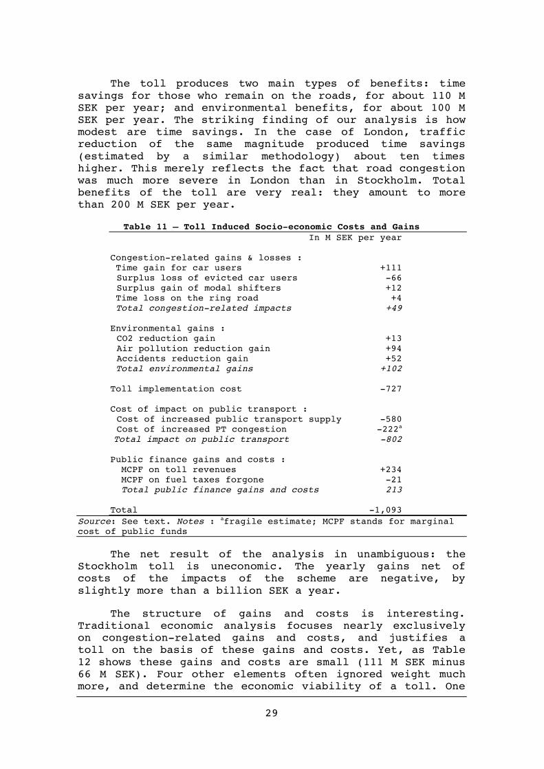
The toll produces two main types of benefits: time savings for those who remain on the roads, for about 110 M SEK per year; and environmental benefits, for about 100 M SEK per year. The striking finding of our analysis is how modest are time savings. In the case of London, traffic reduction of the same magnitude produced time savings (estimated by a similar methodology) about ten times higher. This merely reflects the fact that road congestion was much more severe in London than in Stockholm. Total benefits of the toll are very real: they amount to more than 200 M SEK per year.
Table 11 – Toll Induced Socio-economic Costs and Gains In M SEK per year Congestion-related gains & losses : Time gain for car users +111 Surplus loss of evicted car users -66 Surplus gain of modal shifters +12 Time loss on the ring road +4 Total congestion-related impacts +49 Environmental gains : CO2 reduction gain +13 Air pollution reduction gain +94 Accidents reduction gain +52 Total environmental gains +102 Toll implementation cost -727 Cost of impact on public transport : Cost of increased public transport supply -580 Cost of increased PT congestion -222a
Total impact on public transport -802 Public finance gains and costs : MCPF on toll revenues +234 MCPF on fuel taxes forgone -21 Total public finance gains and costs 213 Total -1,093
Source: See text. Notes : afragile estimate; MCPF stands for marginal cost of public funds
The net result of the analysis in unambiguous: the Stockholm toll is uneconomic. The yearly gains net of costs of the impacts of the scheme are negative, by slightly more than a billion SEK a year.
The structure of gains and costs is interesting. Traditional economic analysis focuses nearly exclusively on congestion-related gains and costs, and justifies a toll on the basis of these gains and costs. Yet, as Table 12 shows these gains and costs are small (111 M SEK minus 66 M SEK). Four other elements often ignored weight much more, and determine the economic viability of a toll. One
30
is environmental costs, for about 100 M SEK. A second relates to the implementation costs of the toll system, for more than 700 M SEK. Economists tend to assume away this “transaction costs”, as if imposing a toll was costless: it is not. The fact that this cost will most probably decline over time with technical progress does not make it possible to ignore that in the Stockholm experiment, this cost is very high. A third item, also usually neglected in theoretical analysis, consists of the economic costs imposed by modal shifters upon the public transportation system. In Stockholm, it amounts to about 800 M SEK per year, including a questionable estimate of the welfare loss associated with a degradation of public transport quality. A fourth item is linked to the toll proceeds. These proceeds are directly neither a gain or a cost, but assuming they reduce taxes, the marginal cost of public funds forgone is a gain, for more than 200 M SEK.
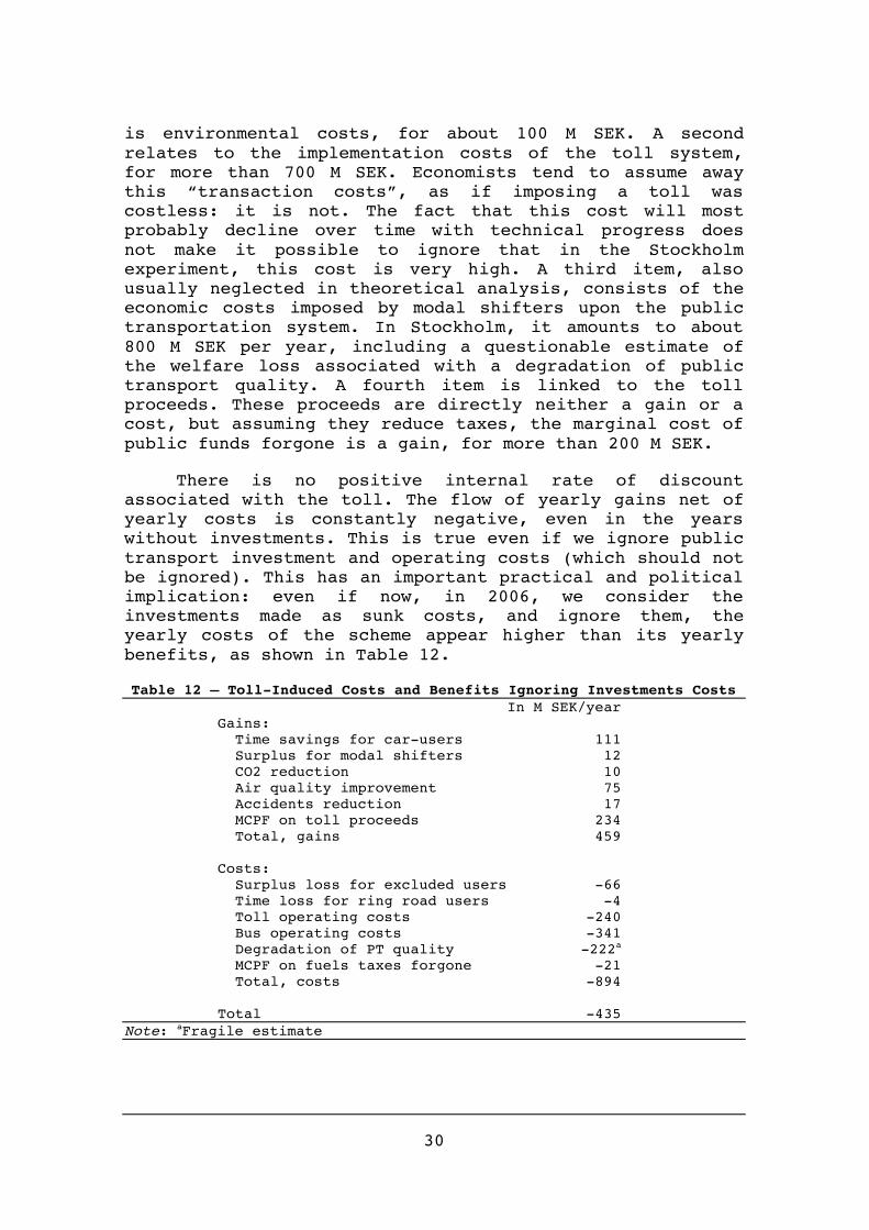
There is no positive internal rate of discount associated with the toll. The flow of yearly gains net of yearly costs is constantly negative, even in the years without investments. This is true even if we ignore public transport investment and operating costs (which should not be ignored). This has an important practical and political implication: even if now, in 2006, we consider the investments made as sunk costs, and ignore them, the yearly costs of the scheme appear higher than its yearly benefits, as shown in Table 12.
Table 12 – Toll-Induced Costs and Benefits Ignoring Investments Costs In M SEK/year Gains: Time savings for car-users 111 Surplus for modal shifters 12 CO2 reduction 10 Air quality improvement 75 Accidents reduction 17 MCPF on toll proceeds 234 Total, gains 459 Costs: Surplus loss for excluded users -66 Time loss for ring road users -4 Toll operating costs -240 Bus operating costs -341 Degradation of PT quality -222a MCPF on fuels taxes forgone -21 Total, costs -894 Total -435 Note: aFragile estimate
31
X — Conclusions
Our analysis remains provisional and tentative. Much work remains to be done. Many of the numbers we use, on traffic reductions, on speeds, on public transport supply costs, on accidents costs, etc. are relatively fragile, and will be improved in the coming months, when all the data collected has been processed. An effort should be made to try and evaluate the cost of a deterioration of service levels in public transportation. One could also try to distinguish between peak and non-peak periods. It would also be important to try to assess the distribution of the various gains and costs amongst different income groups or different geographical areas. It must also be clear that we have only focused on short-terms effects, deliberately ignoring the impacts the toll might have on location patterns. In spite of all these shortcomings, our analysis authorizes some conclusions.
The Stockholm toll experiment offers a unique occasion to evaluate an important policy instrument, and one that justly receives a great deal of attention. In theory, a toll is fully justified to reduce road transport externalities in an urban area to an optimal level. The analysis shows that it does so indeed in Stockholm —and that theory is right. Traffic was reduced by the toll, speeds were increased, and time was saved. The analysis also shows that the toll level chosen is too high, and overreduces car traffic, but this is not very important. More important is the fact that the costs generated by the toll in the case of Stockholm happen to be much higher than the time benefits of the toll. Even if we add, on the benefit side, environmental gains, and the marginal cost of public funds on toll proceeds, total costs are at least three times higher than benefits. Stockholm would have been be much better off —by more than one billion SEK per year— without the toll.
The question asked to the residents of Stockholm is different. It is whether the experiment, now that costly investments have been made, should be continued or terminated. The answer could be “yes”, even though the answer to the question about the economic justification of the toll is “no”. Consider a bridge costing 1,000 to build, 5 per year to operate and maintain, and producing a social utility of 20 per year. Building such a bridge is a waste of scarce social resources and an obvious mistake. But blowing it up once it is built would also be an obvious mistake.
32
Table 12, however, suggests that this is not the case in Stockholm. Even if investment costs are ignored, yearly costs outweight yearly gains. The operation costs of the toll (240 M SEK), the operating costs of the buses (340 M SEK) and the welfare loss associated with the degradation of public transport service quality (220 M SEK) are much greater than the gain in time and in environmental benefits. The difference, however, is not as large as in the “full” case (with investment costs included).
This, by the way, casts a doubt on the nature and meaning of the vote. The vote is presented as a test of people’s attitude relative to urban tolling. A “yes”, it is claimed, will mean that the electorate —the final judge— is in favor of tolls; a “no” that it is against it. This sounds simple and democratic. In reality, it is not. The vote is loaded with at three or four mismatches or ambiguities.
The first one, just mentioned, is about time. On the one hand, the vote is presented as a vote on the toll, or on the toll experiment, in general, as if the decision contemplated was to have a toll or not. But on the other hand, it is presented as (and in reality it is) a vote on the continuation of an existing toll, and voters are invited to ignore the “sunk” investment costs, which happen to be the main part of the toll costs. How will vote someone who is against the toll but is in favor of its continuation? And how will his vote be interpreted? There is an element of arms twisting in deciding first on an investment and then asking the electorate whether this investment should be used or destroyed.
The second one is about space. In a democratic, decentralized setting, the voters should be those who enjoy the benefits and bear the costs, and know better than anybody else what is good or bad for them. This is not what we have in Stockholm. Most of the gains (time gains, environmental gains1) and some of the costs accrue to Stockholm municipality residents, whereas most of the costs are borne by the Swedish national taxpayer (the heavy initial investment cost and a significant share of operation costs), and by residents living outside the Stockholm municipality (welfare loss of evicted car users). Think of a toll area resident who benefits from the toll, but finds it a waste of scarce national public finance resources. Will he vote a selfish “yes” or an altruistic “no”? And how will his vote be interpreted?
1Except for CO2 reduction gains.
33
A third ambiguity has to do the perimeter of the issue submitted to the vote. Is it about the toll, or is it about a combination of toll and public transportation? In principle, a toll has its justification in itself: it reduces traffic and congestion to an optimal level, improving overall welfare. In practice, however, it is difficult to divorce the toll from public transport policies. It is not done in the case of Stockholm. Public transport supply improvements have been made (even if they have apparently been insufficient), and it is stated or suggested that they are “financed” by the toll. This statement (or suggestion) is unjustified. Public revenues are obviously fungible, and the additional revenues provided by the toll could have been used for any other purpose. Increasing public transport supply may well be the best use that can be made of additional public revenues. Or not. This is an interesting debate, and one on which the views of the electorate can usefully be asked. But it is completely distinct from the nature of the tax that is producing these additional revenues.
Another ambiguity is political. The referendum on the toll will be coupled with —and therefore “polluted” by— political elections. Political parties happen to be sharply divided on the toll, with some parties asking voters to say “yes” and other parties asking voters to say “no”. It will be difficult for someone who is against the toll and simultaneously for a party that favors the toll to vote “no” (and vice-versa). Many people will be torn between their party loyalty and their views on the toll.
The present analysis has been static. The gap we find between costs and gains would be reduced if traffic —and in the absence of a toll, congestion— were to increase, and could quickly be reversed. Annex A explores this dynamics. A 30% increase in demand, generated by a 3% growth rate over 10 years or a 2% growth rate over 15 years, would produce, with an optimal toll of 10.3 SEK per trip, a net gain of 145 M SEK (230 M SEK in time gain minus an 85 M SEK in surplus loss). Over time, the value of time would also increase, increasing further this congestion gain. In addition, environmental gains would also increase. So would toll proceeds, and the associated marginal cost of public funds saved. By 2020, the toll would probably be generating social benefits, although much would depend upon the marginal cost of public transportation supply.
Presently, however, the Stockholm experiment does not appear economically justified, and can be considered as a waste of scarce resources. This negative conclusion does
34
not necessarily condemn the idea of urban toll. Our appraisal help understand the conditions required for an urban toll to be really welfare improving.
A first condition is severity of road congestion. In an urban area with very severe traffic conditions, widespread congestion and very low speeds, the benefits of reducing congestion to its optimal level will be much greater. The comparison of London and Stockholm is illustrative in this regard. The benefits achieved by reducing traffic by about 15% are about ten times larger in London than in Stockholm —simply because London was much more congested than Stockholm.
A second condition is low implementation costs. Collecting tolls from millions of car drivers (the number in both Stockholm and London is about 40 million operations per year), checking or double-checking, pursuing delinquents, etc. is necessarily costly. Undoubtedly, technical progress and experience will drive these costs down, perhaps very rapidly. Already, Stockholm costs are about half London costs. For the time being, they nevertheless, even in Stockholm, remain high.
A third condition is cheap public transportation. Evicting car users might be desirable from an environmental and congestion viewpoint. But some of the evicted car users (about half in the case of Stockholm) will shift to public transportation. This will either deteriorate conditions in public transportation or require an increase in public transportation supply (or both, as in the case of Stockholm). The cost of these two outcomes —the marginal cost of public transportation— will vary greatly from city to city. The lower they are, the more attractive the toll. These costs happens to be high in the case of Stockholm.
It appears that these conditions were not fully met in the case of Stockholm. There must be, or there will be in the future, places where they are met, and where an urban toll would be better justified than in Stockholm to-day.
References
Booz Allen Hamilton. 2003. Transport Demand Elasticities Study. Canberra Department of Urban Services (www.actpla.act.gov.au/plandev/transport/ACTElasticityStudy_FinalReport.pdf).
Litman, Todd. 2006. Transportation Elasticities How Prices and Other Factors Affect Travel Behavior. Victoria Transport Policy Institute. 62p. (www.vtpi.org/elasticities.pdf)
Prud’homme, Rémy & Juan Pablo Bocarejo. 2005. « The London Congestion Charge : A Tentative Economic Appraisal ». Transport Policy, vol.12, n° 3, pp. 279-88.
Prud'homme, Rémy. 1999. "Les coûts de la congestion dans la région parisienne". Revue d'Economie Politique. 109 (4), Juillet août 1999, pp. 426-441.
Stockholmsforsöket. 2006. Facts and Results from the Stockholm Trial First version June 2006. 128p
Annex A — When will a Toll Become Justified in Stockholm ? A Dynamic Analysis of Congestion in Stockholm
Our analysis of congestion and congestion reduction has been static. But the model used can also be utilized in a dynamic fashion, to explore what would (or will) happen if and when the demand for road usage in Stockholm increases.
An increase in demand caused by non-price reasons, such as an increase in total population or activity in the Center, or an increase in income, or an increased preference for car travel, or a deterioration of public transport conditions, etc. will lead to a shift of the demand curve to the right (as opposed to the shift on the demand curve induced by a toll).
36
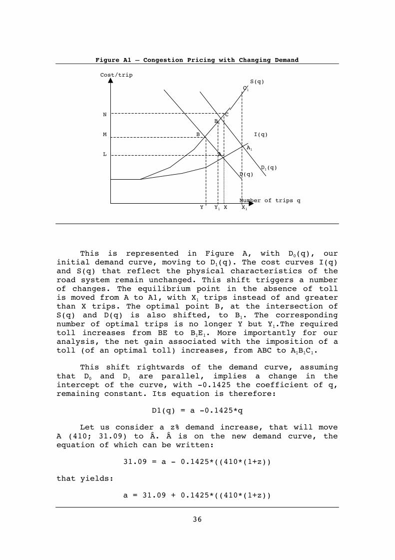
Figure A1 – Congestion Pricing with Changing Demand Cost/trip S(q) C1 N C B1 M B I(q) A1 L A D1(q) D(q) Number of trips q Y Y1 X X1
This is represented in Figure A, with D0(q), our initial demand curve, moving to D1(q). The cost curves I(q) and S(q) that reflect the physical characteristics of the road system remain unchanged. This shift triggers a number of changes. The equilibrium point in the absence of toll is moved from A to A1, with X1 trips instead of and greater than X trips. The optimal point B, at the intersection of S(q) and D(q) is also shifted, to B1. The corresponding number of optimal trips is no longer Y but Y1.The required toll increases from BE to B1E1. More importantly for our analysis, the net gain associated with the imposition of a toll (of an optimal toll) increases, from ABC to A1B1C1.
This shift rightwards of the demand curve, assuming that D0 and D1 are parallel, implies a change in the intercept of the curve, with -0.1425 the coefficient of q, remaining constant. Its equation is therefore:
D1(q) = a -0.1425*q
Let us consider a z% demand increase, that will move A (410; 31.09) to Â. Â is on the new demand curve, the equation of which can be written:
31.09 = a - 0.1425*((410*(1+z))
that yields:
a = 31.09 + 0.1425*((410*(1+z))
37
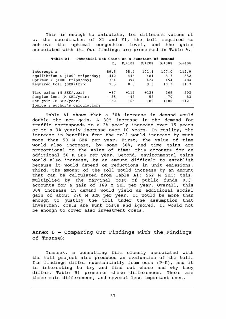
This is enough to calculate, for different values of z, the coordinates of X1 and Y1, the toll required to achieve the optimal congestion level, and the gains associated with it. Our findings are presented in Table A.
Table A1 – Potential Net Gains as a Function of Demand D0 D0+10% D0+20% D0+30% D0+40% Intercept a 89.5 95.4 101.1 107.0 112.9 Equilibrium X (1000 trips/day) 410 446 481 517 552 Optimum Y (1000 trips/day) 364 394 424 454 484 Required toll (SEK/trip) 7.5 8.5 9.3 10.3 11.3 Time gains (M SEK/year) +87 +112 +138 169 203 Surplus loss (M SEL/year) -35 -48 -58 -70 -83 Net gain (M SEK/year) +50 +65 +80 +100 +121 Source : author’s calculations
Table A1 shows that a 30% increase in demand would double the net gain. A 30% increase in the demand for traffic corresponds to a 2% yearly increase over 15 years or to a 3% yearly increase over 10 years. In reality, the increase in benefits from the toll would increase by much more than 50 M SEK per year. First, the value of time would also increase, by some 30%, and time gains are proportional to the value of time: this accounts for an additional 50 M SEK per year. Second, environmental gains would also increase, by an amount difficult to establish because it would depend on reductions in unit emissions. Third, the amount of the toll would increase by an amount that can be calculated from Table A1: 562 M SEK; this, multiplied by the marginal cost of public funds 0.3, accounts for a gain of 169 M SEK per year. Overall, this 30% increase in demand would yield an additional social gain of about 270 M SEK per year. It would be more than enough to justify the toll under the assumption that investment costs are sunk costs and ignored. It would not be enough to cover also investment costs.
Annex B – Comparing Our Findings with the Findings of Transek
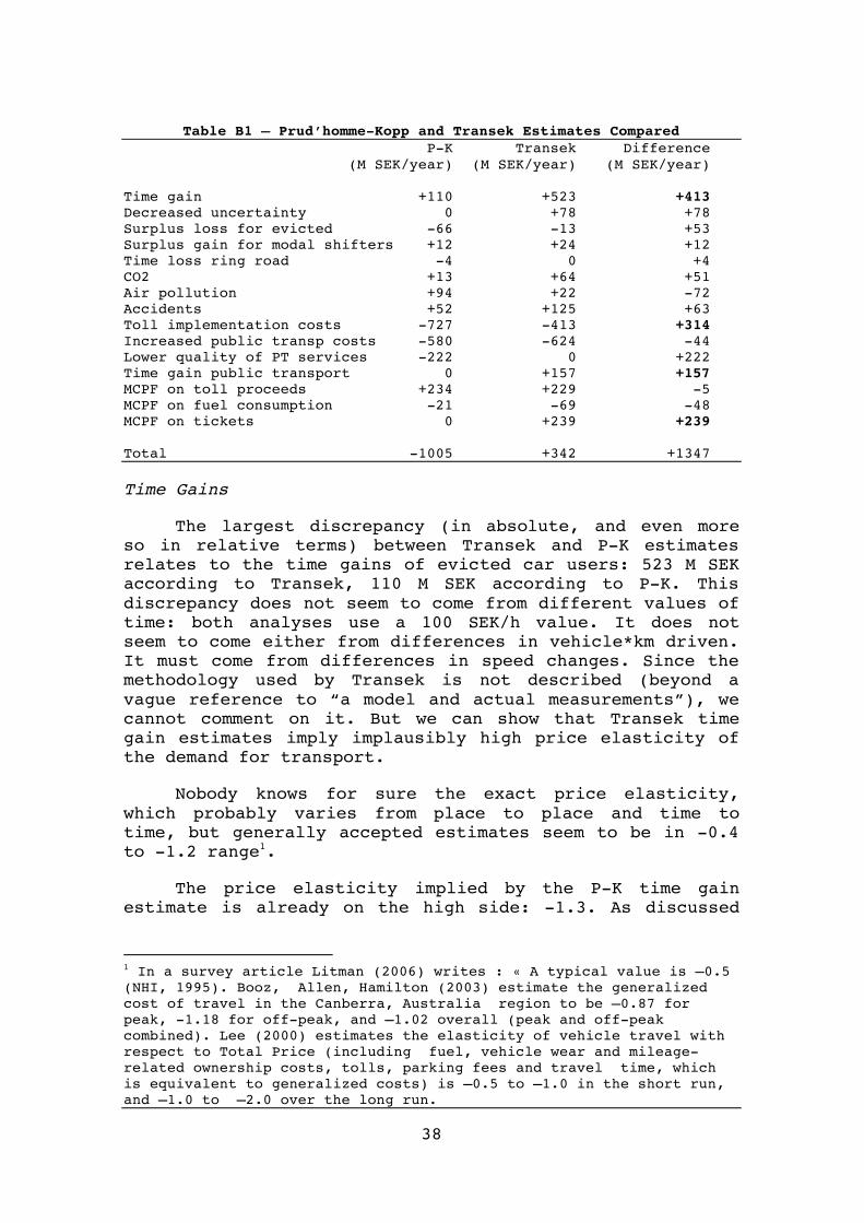
Transek, a consulting firm closely associated with the toll project also produced an evaluation of the toll. Its findings differ substantially from ours (P-K), and it is interesting to try and find out where and why they differ. Table B1 presents these differences. There are three main differences, and several less important ones.
38
Table B1 – Prud’homme-Kopp and Transek Estimates Compared P-K Transek Difference (M SEK/year) (M SEK/year) (M SEK/year) Time gain +110 +523 +413 Decreased uncertainty 0 +78 +78 Surplus loss for evicted -66 -13 +53 Surplus gain for modal shifters +12 +24 +12 Time loss ring road -4 0 +4 CO2 +13 +64 +51 Air pollution +94 +22 -72 Accidents +52 +125 +63 Toll implementation costs -727 -413 +314 Increased public transp costs -580 -624 -44 Lower quality of PT services -222 0 +222 Time gain public transport 0 +157 +157 MCPF on toll proceeds +234 +229 -5 MCPF on fuel consumption -21 -69 -48 MCPF on tickets 0 +239 +239 Total -1005 +342 +1347
Time Gains
The largest discrepancy (in absolute, and even more so in relative terms) between Transek and P-K estimates relates to the time gains of evicted car users: 523 M SEK according to Transek, 110 M SEK according to P-K. This discrepancy does not seem to come from different values of time: both analyses use a 100 SEK/h value. It does not seem to come either from differences in vehicle*km driven. It must come from differences in speed changes. Since the methodology used by Transek is not described (beyond a vague reference to “a model and actual measurements”), we cannot comment on it. But we can show that Transek time gain estimates imply implausibly high price elasticity of the demand for transport.
Nobody knows for sure the exact price elasticity, which probably varies from place to place and time to time, but generally accepted estimates seem to be in -0.4 to -1.2 range1.
The price elasticity implied by the P-K time gain estimate is already on the high side: -1.3. As discussed
1 In a survey article Litman (2006) writes : « A typical value is –0.5 (NHI, 1995). Booz, Allen, Hamilton (2003) estimate the generalized cost of travel in the Canberra, Australia region to be –0.87 for peak, -1.18 for off-peak, and –1.02 overall (peak and off-peak combined). Lee (2000) estimates the elasticity of vehicle travel with respect to Total Price (including fuel, vehicle wear and mileage-related ownership costs, tolls, parking fees and travel time, which is equivalent to generalized costs) is –0.5 to –1.0 in the short run, and –1.0 to –2.0 over the long run.
39
in the text, if we use the value of time for private car users, this price elasticity is reduced to -0.9.
If the value of time gains generated by the toll is 523 M SEK, as estimated by Transek, then the toll-generated additional cost or price to users is 270 M SEK per year. It is equal to 3.3 SEK per trip. This represents 4.2% of the average generalized cost of a trip. It is difficult to believe that such a small price increase could generate the 19.8% decline in car usage assumed by Transek. It would imply a –4.7 price elasticity of car transportation, well beyond commonly accepted values of short-term (and even long-term) elasticities. Actually, things are even worst than that. Transek estimates the gain of more predictable car trips at 78 M SEK per year. This is to be added to the 523 M SEK per year time gain. It yields a 2.3 SEK per trip price increase (toll minus gain), representing a relative increase of the average trip of about 3%. For this (net) price increase to reduce car usage by nearly 20%, a -6.6 price elasticity would be required.
Toll Implementation Cost
The second largest difference relates to toll implementation costs: 727 M in P-K, 413 M in Transek. There is a broad agreement on the magnitude of investment costs and of operating costs (1,830 M SEK for investments, and 240 M SEK for yearly operating costs). The disagreement is on the treatment of investment costs.
Transek assumes that the investment should be amortized on a 40 years period, or to put it otherwise, that no additional investment would be required by the operation of the toll in the next 40 years. The required hardware repairs and replacement and software modifications would be covered by the operation costs.
P-K, by contrast, treat this investment the way an ordinary industrial or commercial enterprise would treat it, and amortize it over a much shorter period. Considering the mix of computer-type material (usually amortized over a 3 years period) and more standard material (amortized over a 10 years period), they adopted a 6 years amortization period. We asked Vinci, an important French group operating toll facilities in many countries, what their amortization practices —sanctioned by chartered accountants, tax administrations and regulatory agencies in these many countries— are: the answer was 6-7 years. We also tried to find out what Capita, the private company that operates the London toll
40
does. It seems that it initially used a 5 years depreciation period, later changed into a 7 years period.
Public Transport Gains/Costs
The third largest discrepancy between P-K and Transek comes from the public transport additional fares, which are counted as a benefit by Transek, for 239 M SEK per year. Fares may be a gain for the public transport company, but they are a cost to fare payers: they are not an economic gain to society, a decrease in the consumption of scarce economic resources or an increase in consumer’s satisfaction. What is an economic gain is the consumer’s surplus of the modal shifters, estimated elsewhere by Transek and by P-K (these estimates differ but they are small).
Transek also counts as a gain the time saved by public transport users, for 157 M SEK per year. In principle, this would be acceptable. In practice, it is questionable. This gain could only concern bus transportation, as opposed to train and subway transportation, and bus transportation is not the main part of public transportation. Since the toll increased speeds on the roads, buses should be driving faster, and bus users gaining time. It is probably modest, because SL did not change its bus schedules, and because much of the time spent by bus users in buses is spent in buses slowing down, stopping and accelerating, so that they do not benefit much from increased flow traffic. In London, Transport for London estimated that bus speed increases were about half car speed increases (which were much more important than in Stockholm). Stockholmsforsöket (2006, p. 49-50) reports and provides a map showing that “average [bus] speeds throughout most of the trunk road network during the peak morning hour from 7.30-8.30 is unchanged or has improved/deteriorated by a maximum of one km/hour”.
Evaluating the impact of a toll on public transportation is part of the evaluation of a toll. Some (about half in the case of Stockholm) of the evicted car users shift to public transportation. If the supply of public transportation remains constant, this will result in a deterioration of service quality that has a cost (difficult to estimate, but potentially significant: the deterioration may be small, but the number of public transport users suffering from it is large). If the supply of public transportation is increased, so as to keep service levels constant, this will be done at a cost. There is obviously a relationship between these two types of costs: the greater the cost of increased supply, the
41
lower the cost of deterioration (which might even become negative, i.e. reflect an improvement in service quality), and there must be an optimal combination of the two. In the case of Stockholm, we know that there has been an increase in transport supply that took the form of an additional 200 buses, at a cost and that there has been an overall deterioration of service levels.
Transek completely ignores this overall deterioration, but values the welfare gain generated by the additional 200 buses, and deducts this value from the cost of supplying these 200 buses. This is assuming away the toll. If there had been no toll, the 200 buses would indeed have generated a welfare gain for their users. SL surveys would show an increase in satisfaction levels, and in the ratios of standing travelers. But there has been a toll, that generated modal shifters, increased pressure on the system, and led to a clear deterioration of service levels. We do not deny the welfare gain produced by the additional buses, but remark that it must have been more than compensated by the welfare loss experienced in the rest of the system. The net impact of additional buses and modal shifting on public transport users surplus has been negative: Transek procedure turns it into something positive !
P-K are aware that their estimate of this net negative impact is fragile —and they state it. But there is no doubt that it is negative. And a fragile estimate is probably closer to the truth that a zero estimate.