J . Fluid Mech. (1981), vol. 113, p p 75-90

Printed in Great Britain 75

The structure of a separating turbulent boundary layer. Part 3. Transverse velocity measurements

By K. SHILOH,? B. G. SHIVAPRASAD A N D R. L. SIMPSON

Southern Methodist University, Dallas, Texas 75275

(Received 19 August 1980 and in revised form 16 March 1981)

Simpson, Chew & Shivaprasad (1981 a , b) describe many experimentally determined features of a separating turbulent boundary layer. For the same flow, experimental results for the transverse velocity component are presented here. A specially designed directionally sensitive laser anemometer was constructed and used to make measure- ments in the separated region. Cross-wire hot-wire anemometer measurements were obtained upstream of separation and in the outer region of the separated flow and are in good agreement with the laser anemometer results.

It was found that wI2 = v t2 in the outer 90 yo of the shear layer both upstream and downstream of separation. Features of wI2 profiles in the backflow are related to features of the streamwise velocity component. This behaviour is consistent with the large-scale-structures flow model of a separating boundary layer presented by Simpson et al. (1981a, b ) .

Large-scale structures supply the mean streamwise backflow. These large-scale structures also transport the turbulence energy to the backflow from the outer flow by turbulent diffusion since advection and production of turbulence kinetic energy are negligible there compared with the dissipation rate. Because of continuity require- ments fluid motions toward the wall must be deflected and contribute to streamwise and transverse motions near the wall.

1. Introduction Simpson et al. (198la, b ) presented experimental results for a nominally two-

dimensional separating turbulent boundary layer for an airfoil-type flow in which the flow was accelerated and then decelerated until separation. Upstream of separation single- and cross-wire hot-wire anemometer measurement results were presented. Measurements were obtained in the separated zone with a directionally sensitive laser-anemometer system for mean velocities U and 77 and characteristics of the fluctuation velocities u and v: u2, v2, -uV, u3, v3, u4, v4, the fraction of time that the flow moves downstream y1,?,, fraction of time that the flow moves away from the wall ypr, and u spectra.

For the same flow this paper presents experimental results along the tunnel centre- line for the transverse mean velocity W and characteristics of the transverse fluctua- tion velocity w: w2, w3 and 2. A specially designed, directionally-sensitive laser

t Permanent address : Israel Atomic Energy Commission, Soreq Nuclear Research Couter,

- - - - - -

- -

Yavne, Israel 70600.

76 K . Shiloh, B. G . Shivaprasad and R. L. Simpson

anemometer was constructed and used to make measurements in the separated region. Cross-wire hot-wire anemometer measurements were obtained upstream of separation and in the outer region of the separated flow. The next section describes this experimental equipment. Section 3 describes the experimental results and 9 4 discusses the meaning of these results. Section 5 presents thc implications of these results on our understJanding of the nature of the instantaneous velocity W ( = W + w ) in a separating turbulent boundary layer.

2. Experimental equipment Simpson et al. (1981a, b) used and decribe in some detail the same wind tunnel,

boundary-layer control system, and test flow as used in the current series of experi- ments. The description of these aspects will not be repeated here since the results presented here supplement the earlier results. I n other words, all three papers are required to obtain all of the measurement results on the test flow.

The same hot-wire anemometers and electronics as used by Simpson et al. (1981 a, b) were used in this research. However, the probe and the alignment technique required for satisfactory W measurements are sufficiently different to warrant further dis- cussion. An entirely new laser-anemometer optical arrangement was required to measure W, as described below.

2.1. Hot-wire anemometer probe The hot-wire probe was a standard TSI Model 1248-T1.5 end-flow miniature cross- wire probe. Each wire is inclined a t 45" to its sensor supports. I n use one wire is sensi- tive to u + w fluctuations while the other is sensitive to u - w. The probe stem or the 0.06 in. outside diameter stainless-steel tube containing the sensor supports was mounted perpendicular to the probe holder and permitted measurements as close as 0.05 in. from the surface. The two platinum-plated tungsten-wire sensors, 0-00015 in. diameter and 0.05 in. long, are only 0.02 in. apart, which produces less effect of large streamwise velocity gradients on the measurements than wider spacings. Each linearized calibration had a small deviation from a straight line, with a product moment correlation coefficient (Bragg 1974) in excess of 0.9999. The slopes of each calibration were repeatable within k 4 % over the entire series of experiments.

A TSI Model 1015C Correlator was used to add and subtract instantaneously the linearized u + w and u - w signals obtained from the two wires. Two Analog Devices AD533JH four-quadrant multipliers were used, one in the squaring mode and the other in the multiplying mode to obtain u2, w2, ( U + W ) ~ , ( u - w ) ~ , w3 and w4. The nonlinearity error for the multipliers was approximately & 2 yo of the full-scale output voltage of 10 V2. The time-averaging was done using true-integrating voltmeters consisting of a voltage-controlled oscillator (Tektronics FG501 and Wavetek Model 131) and a digital frequency counter (Tektronics DC 503 Universal Counter and Anadex CF-600). Measurements with the true-integrating voltmeters were repeatable within k 1 %. The overall frequency response of the hot-wire anemo- meter and its associated instrumentation was flat up to 7.5 kHz.

To align the sensors properly with respect t o the probe holder, the plane formed by the probe stem and the probe holder was mounted perpendicular to the calibrator flow. The probe stem was rotated within the hole in tjhe probe holder until the voltages

Structure of a separating turbulent boundary layer. Part 3 77

obtained from both wires were a minimum. Thus, both wires were inclined a t 45" to the calibration flow direction. The set-screw was tightened to lock the probe stem to the probe holder in that position. This process ensured that each wire was in the xz plane when the probe holder was aligned with the y direction.

To ensure that the probe stem axis and hence the planes containing the two wires are parallel t o the 2 axis in the test flow, the probe was mounted in the wind tunnel such that the sensors were close to the bottom test wall. Since the bottom wall was a highly polished wooden surface the reflected image of the probe stem was visible to the naked eye. The probe holder fixed to the traversing mechanism was rotated about the z axis auch that the stem and its image were visibly parallel. Finally, to ensure that both the wires were inclined to the x direction a t 45", the probe was moved to the free stream and the probe holder was rotated about the y axis until the velocities obtained from the individual signals and the sum of the two signals were within 1 % of one another .

I n summary, the uncertainties for the hot-wire measurements due to all of these sources are: U , k 3 %; u2, k 8.2 %; 2, k 12.5 %; skewness factor X,, 2 0.1; flatness factor Fw, k 1.0; - UUI, k 1 (ft s - ~ ) ~ . Measurements in the separated region were con- fined to regions where the instantaneous flow direction made an angle less than 45" with the mean flow direction.

A motorized traversing mechanism as described by Strickland & Simpson (1973) was used for traversing the X-wire probe across the boundary layer. It had a probe positioning uncertainty of 2 0.001 in. In addition, a cathetometer was used to locate the probe sensor near the wall within an uncertainty of approximately k 0.002 in.

-

2.2. Laser anemometer The basic requirements of a W component laser anemometer are that it be direction- ally sensitive, that it have high y-direction spatial resolution, and that i t have high enough signal-to-noise ratio and signal data rate to produce well-defined velocity probability histograms. Ideally one would like to add the W component measuring system to the existing $2 and V measuring system described by Simpson & Chew (1979) and Simpson et al. (1981 a ) and use the same optical window in the wind tunnel as used for 92 and Y measurements.

This is only possible using a reference beam approach where the incident laser beam is parallel to the Wdirection. Orloff & Logan (1973) and Kreid & Grams (1976) have developed such confocal backscattering reference beam anemometers. However, they require an etalon to increase the coherence length of the laser and a good optical table for precise alignment of the received signal and the reference beam.

A second approach is a dual beam system where the incident laser beams enter through the wind-tunnel bottom and form real fringes that are perpendicular to the W direction. This approach has all of the advantages of a fringe system over a reference beam system; it permits a large received signal aperture, produces higher signal-to- noise ratio (SNR) signals for sparse seeding, does not require critical beam alignment to obtain good signals, does not require an etalon as long as incident beam paths are equal, and does not require a high quality optical table. Figure 1 is a schematic diagram of this approach, which was used to obtain the results presented here.

The length of the signal-producing focal volume was too long to obtain the required y-direction spatial resolution using forward or back scattering. Thus, the signal was

78 K . Shiloh, B. G. Shivaprasad and R. L. Simpson

FIGURE 1 . Schematic diagram of the side view of the fringe-type laser anemometer used to measure W. A , aperture, slit or iris; B, Bragg cell; F , 0.488 mm wavelength filter; Li, lenses; M , , adjustable mirrors; M,, beam folding mirrors; 0, optical flat; P , photomultiplier; S, sampling volume; W , wind-tiinnel windows.

collected at right angles to the incident beams as shown in figure 1 . The photo- multiplier tube aperture was opened enough to obtain signals from only a small portion of the focal volume height.

Since the measuring volume in this optical arrangement is governed by the focal volume diameter, primary consideration in the optical system design was given to obtain a focal volume diameter that produced good SNR signals a t a sufficiently high rate. Too large a focal volume diameter produces too low SNR signals owing t o laser power limitations. On the other hand, too small a focal volume diameter produces too low a signal data rate owing to a too small number of particles in the focal volume. An intermediate diameter was selected that produced both a high SNR and a good signal data rate. As shown in figure 1, lenses L, and L, and the final focusing lens L, were used to determine the beam diameter and to produce parallel ray beams that crossed a t the focal volume. This produced parallel fringes without requiring that the two beams cross at their waists as in the case of converging-ray beams. The Bragg cell split the initial laser beam into two equal power beams with one frequency shifted 24.55 MHz. This produced fringes that moved through the focal volume a t the Bragg- shifted frequency and made the laser anemometer directionally sensitive. In other words, W motions in one direction produced signals greater than the Bragg frequency while Wmotions in the other direction produced signals less than the Bragg frequency.

Aside from the mirrors that manipulate the laser beams, the only other important component in the incident beams system is the optical flat. As shown in figure 1, rotation of the optical flat about the vertical axis permits sensitive streamwise adjust- ment of one of the incident laser beams so that the plane of the laser beams can be aligned with the $bT velocity component. Proper alignment is achieyed when W is repeat ably zero well within the experimental uncertainty.

The signal-receiving lens L,, photomultiplier tube, and interference filter are the

Structure of a separating turbulent boundary layer. Part 3 79

same as used by Simpson & Chew (1979) and Simpson et al. ( 1 981 a ) . A slit or an iris diaphragm was used as the aperture. Near the wall where aU/ay is large, the dioctyl phthalate smoke particle coilcentration is sufficiently high that a horizontal slit of height 0.01 in. provides a good signal data rate and good spatial resolution. Farther away from the wall the smoke concentration is lower and aU/ay is lower so that the iris with up to 0.08 in. opening can be used.

Signal processing was by fast-sweep-rate sampling spectrum analysis, with the same equipment as described by Simpson & Barr (1975) and Simpson & Chew (1979) and used by Simpson et al. (1981 a) . The output voltage from the signal processor was fed to a probability analyser where a velocity probability histogram was obtained. W , w2, w3, w4, and the fraction of time that the W flow is positive, yPw, can be obtained from each histogram. As pointed out by Simpson & Chew (1979) and Simpson et al. (1981 a ) , the equal-time-interval sampling by the probability analyser of the sample- and-hold signal processor output voltage results in a true-time-averaged histogram shape rather than an average over the number of signals obtained.

The signal must be distinguishable above the wideband noise level for detection. The discrimination level must be above the highest noise level present in the range of Doppler frequencies for the turbulence present. Since the signal is processed in the frequency domain, the signal-to-wideband-noise ratio need not be as good as signals processed in the time domain with counters. A resolution bandwidth of 1 to 3 yo of the frequency analyser dispersion and a sweep rate between 200 and 1000 Hz was used. The sweep rate was set equal to the sampling rate of the probability analyser. For most of these experiments, the discrimination level was set at 8 dB, permitting a data signal rate of 100-200 Hz.

The 1 ,um dioctyl phthalate particles follow the highly turbulent oscillations found in separated regions (Simpson & Chew 1979). It is, of course, impossible to seed a highly turbulent flow in any prescribed manner. This is not really important since equal- time-interval sampling by the probability analyser produces a histogram that is independent of the particle concentration. Based on the estimates given by Echols & Young (1963) there are about 131 000 particles per cubic inch.

At this concentration the number of particles in the volume a t any time varies between 0.13 when using the slit aperture to 0.9 for the iris aperture. These conditions correspond to the loss of signal or dropout 87 or 10 % of the time, respectively. These results are consistent with the observation that a t a 1000 Hz sweep rate the data rate is only 200 Hz to 300 Hz, i.e. signals only occur 20 to 30 yo of the time.

The major source of uncertainty in these measurements is the drift of the spectrum analyser. The influence of this drift on the results calculated from histograms was examined using actual histograms and assuming a flat distribution for the drift. The drift had little practical effect on the variance 2 while the skewness and flatness factors tended to approach Gaussian values.

Other factors produced minor uncertainties. The uncertainty in the angle between the two laser beams and the uncertainty in the spectrum analyser frequency-to- voltage calibration produce an uncertainty of & 2 yo in the instantaneous velocity. Velocity gradients across the focal volume produce a broadening in the histogram of about 0.25 ft2 s - ~ .

I n summary, taking into account all of these sources of uncertainty, the maximum uncertainties for the laser anemometer results reported here are: W , 5 1.5 f t s-l;

---

80

(w2)*, k 0.5 f t s-l; S,, 0.2; F,, k 1.0. The distance of the measurement volume from the test wall is about f 0.002 in. uncertain while the movement of the traversing apparatus is about k 0.001 in. uncertain. These uncertainty estimates are con- sistent with the observed scatter in the results presented in $ 3 below.

K . Shiloh, B. C. Shivaprasad and R. L. Simpson -

3. Experimental! results Representative measurements of W-related quantities were obtained in the several

regions of this flow. Hot-wire anemometer measurements were obtained near the beginning of the adverse pressure gradient region near 64in. Laser and hot-wire anemometer measurement's were obtained a t 115 in. just upstream of the beginning of intermittent separation and at 126 in. in the intermittent separation region. Measurements near 138 in. were obtained for a low mean backflow while those a t 160 and 173 in. are for the well-developed backflow region. These results are tabulated in the appendix of Shiloh, Shivaprasad & Simpson (1980) and are on the magnetic tape with the data of Simpson et al. (1981 a, b).

3.1. Mean velocity results Mean velocities in the longitudinal direction U were measured as a by-product during the measurement of W turbulence quantities with the cross-wire probe. These results agree with the measurements of Simpson et al. (1981a) within the uncertainties of both sets of data.

The angle between the free-stream flow direction and the tunnel centre-line was measured by the hot-wire and laser anemometers. The free-stream flow moved slightly across the tunnel toward the optics. Only downstream of 150 in. was W greater than the W measurement uncertainty. Within the boundary-layer flow W varied randomly about zero within the measurement uncertainties up to the 138 in. location. Down- stream W/Um increased with distance to 0.04 a t 173 in., with an uncertainty of & 0.03.

3.2. Turbulence results The turbulent intensities in the longitudinal direction u'/Um were also obtained as a by-product during the hot-wire measurements. The discrepancy between these data and the Simpson et al. (1981 a ) data lies within the uncertainties a t all stations except the downstream-most one at 173a in. Nevertheless, this general agreement between the two sets of data instills confidence in these hot-wire measurements.

Shiloh et al. (1980) give the lateral turbulent intensity profiles at all the stations using both the laser and the hot-wire anemometers. I n general, the two sets of data agree with one another within their total uncertainty limits a t most locations. How- ever, at 173f in. the agreement is not satisfactory. Still, the good agreement for most of the stations with the established hot-wire technique gives confidence in the dual beam technique of measurement of w' with the laser anemometer.

3.3. Skewness andJEatness factor results Shiloh et al. (1980) give the distributions of the flatness F, and skewness S, factors upstream of separation. There is agreement, between the laser and hot-wire anemo- meter results within the uncertainties. Near the wall F, rises substantially above the

Structure of a separating turbulent boundary layer. Part 3

8 -

6 -

< 4 -

2 -

81

$

2

+ e B 2$

fi

B $ . B B .

I I

0.2

0: 0-

-0.2

-4.4-

-0.6

-0.8

0.4 + e

$ b d

- .. .. $ . B $3 * + fi ~*~b$gg$$&$pp . a B 2 B,"

cr .. c m - $ $+&

% m S . -

G I I I 1 1 1 1 1 1 1 1 I I I

.

Gaussian value of 3, as was the case for ql and F, reported by Simpson et al. (1 98 1 a ) S, is nearly independent of distance from the wall and is slightly positive, although it is within the experimental uncertainty of being zero for a two-dimensional mean flow.

Figures 2 and 3 show the laser-anemometer results downstream of separation. These figures also show the results of Wygnanski & Fiedler (1970) for the low-velocity side of a plane mixing layer. As in the case of the u and v fluctuations (Simpson et al. 1981b) these two types of flow have similar distributions for X, and F,. Also as in the case of t,he u and v fluctuations, X, and Fw tend to achieve profile similarity from

82 K . Shiloh, B. G. Shivaprasad and R. L. Simpson

( a )

O m

0.01 5 x = 125.95 in.

I = 63.81 in. I 0.005

oO.OO1 0.01 0.1 0.3 0.5 0.7 0.9 1.1

Y 16

0.025 0 . 0 3 ~

Y 16

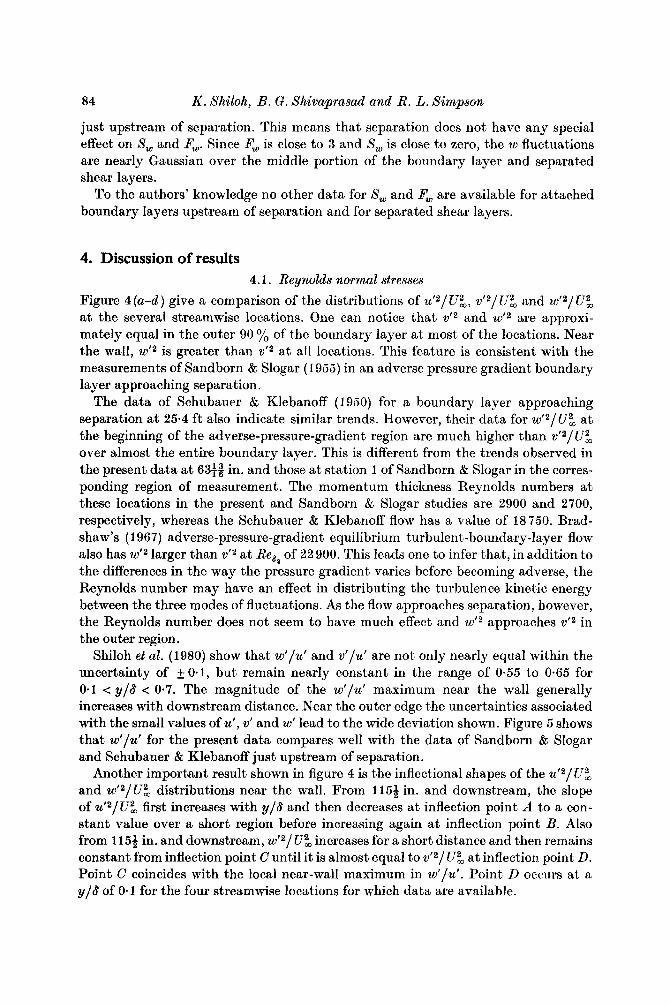
FIGURE 4. Reynolds-normal-stresses distributions ( a ) for several values of z; (b ) for z = 138.7 in.; (c) for z = 160.3 in.; and ( d ) for z = 173.3 in. Simpson et al. (1981a): gS, U ' ~ / U ; ; A, v'"/J;. Q, w f Z / U ~ . Note the log-linear abscissa.

Structure of a separating turbulent boundary layer. Part 3

0.035

0.03

0.025

' 3k

83

-

-

-

0.04 ( d )

B

B

0

B

B

Gb G O , Q b

.1 0.3 0.5 0.7 0.9 Y 16

1

FIGURE 4c, d . For legend see p. 82.

84 K . Shiloh, B. G . Shivaprasad and R. L. Simpson

just upstream of separation. This means that separation does not have any special effect on S, and F,. Since F, is close to 3 and S, is close to zero, the w fluctuations are nearly Gaussian over t,he middle portion of the boundary layer and separated shear layers.

To the authors' knowledge no other data for S, and Fw are available for attached boundary layers upstream of separation and for separated shear layers.

4. Discussion of results 4.1. Reynolds normal stresses

Figure 4(a-d) give a comparison of the distributions of uf2/UuZ,, vf2/UuZ, and w f 2 / l g at the several streamwise locations. One can notice that v ' ~ and wf2 are approxi- mately equal in the outer 90 % of the boundary layer at most of the locations. Near the wall, wf2 is greater than v f 2 a t all locations. This feature is consistent with the measurements of Sandborn & Slogar (1 955) in an adverse pressure gradient boundary layer approaching separation.

The data of Schubauer & Klebanoff (1950) for a boundary layer approaching separation at 25.4 f t also indicate similar trends. However, their data for wt2/ U2, a t the beginning of the adverse-pressure-gradient region are much higher than vf2/ U: over almost the entire boundary layer. This is different from the trends observed in the present data a t 63+$ in. and those at station 1 of Sandborn & Slogar in the corres- ponding region of measurement. The momentum thickness Reynolds numbers at these locations in the present and Sandborn & Slogar studies are 2900 and 2700, respectively, whereas the Schubauer & Klebanoff flow has a value of 18750. Brad- shaw's (1 967) adverse-pressure-gradient equilibrium turbulent-boundary-layer flow also has wI2 larger than v f 2 at Res, of 22 900. This leads one to infer that, in addition to the differences in the way the pressure gradient varies before becoming adverse, the Reynolds number may have an effect in distributing the turbulence kinetic energy between the three modes of fluctuations. As the flow approaches separation, however, the Reynolds number does not seem to have much effect and wt2 approaches vf2 in the outer region.

Shiloh et al. (1980) show that wf/u ' and v f / u f are not only nearly equal within the uncertainty of k0.1, but remain nearly constant in the range of 0.55 to 0.65 for 0.1 c y/S c 0.7. The magnitude of the w' /u f maximum near the wall generally increases with downstream distance. Near the outer edge the uncertainties associated with the small values of u', vf and wf lead to the wide deviation shown. Figure 5 shows that w'/u' for the present data compares well with the data of Sandborn & Slogar and Schubauer & Klebanoff just upstream of separation.

Another important result shown in figure 4 is the inflectional shapes of the u12/U: and wf2/Uu", distributions near the wall. From 115i in. and downstream, the slope of uf2/Uu", first increases with y/6 and then decreases at inflection point A to a con- stant value over a short region before increasing again at inflection point B. Also from 1154 in. and downstream, wI2/ U: increases for a short distance and then remains constant from inflection point C until it is almost equal to vf2/UuZ, at inflection point D. Point C coincides with the local near-wall maximum in w'/u'. Point D occiirs at a y/6 of 0.1 for the four streamwise locations for which data are available.

Structure of a separating turbulent boundary layer. Part 3 85

t A

v

FIGURE 5. w'/u' upstream from detachment. 0, 115.5 in. 0 , Sandborn & Slogar (1955), station 4. Schubaner & Klebanoff (1950): A, 24.3 ft; A, 25.4 ft. Note the log-linear abscissa.

Points C and D also have special significance in regard to profiles of @-related data from Simpson et al. (1981a, b ) . Figure 3 in Simpson et al. (1981a) shows that, down- stream of fully developed separation, point C corresponds closely to the position of minimum mean velocity U . Point D occurs at a slightly higher velocity. Figure 5 in Simpson et al. (1981 a) and Shiloh et al. (1980) show that point C closely corresponds to the minima in the upstream-downstream intermittency ypu and the intermittency of the flow away from the wall ypv. Figure 1 in Simpson et al. (1981 b) shows that points C and D lie on opposite sides of the hump in the flatness factor Fu. The hump itself shows that relatively large u fluctuations occur infrequently in this region, indicating the intermittent passage of very-high- and very-low-velocity fluid with respect to the mean velocity.

Figure 13(c) in Simpson et al. (1981a) shows no special significance for points C and D in - UV/u'v' profiles downstream of separation, except that they lie in the region of increasing correlation of Reynolds-shear-stress-producing u' and v' motions. Point A seems to be near where - UV is first significantly greater than zero.

Figure 13 in Simpson et al. (1981 b) shows the turbulence-energy balance at 156# in, No significant turbulent energy production occurs closer to the wall than point D. The next section relates the near-wall data to the turbulence-energy dissipation rate.

4.2. Turbulence-energy dissipation rate near the wall Some insight about the turbulence-energy balance near the wall can be gained by relating the measured near-wall structure to the turbulence-energy dissipation rate. From the continuity equation and the no-slip condition at the wall, the equations for the velocity fluctuations nearest the wall

u = aly+azy2+.. . , v = b&+ ..., w = ~ ~ ~ + + ~ ~ 2 + . . . (1 )

86 K . Shiloh, B. G. Shivaprasad and R. L. Simpson

Location (in.) sS/UL x 103 ( E / Y ) x 10-7 s2

1384 3.6 4.6 3.7 2.3 4.2 2.3 173&

1166 4.2 23

16@4

TABLE 1. Estimated turbulence-energy dissipation rate a t the wall.

can be written, where a,, a2, b,, c1 and c2 are functions of time. After squaring each side of each equation and time-averaging the result, one obtains

u2 =a!y2+2aIa2y3+a~g4+ ..., v2 = b%y4+ ..., w2= c ] y + 2 c ~ y 3 + c ~ y 4 + . . . . ( 2 )

At the wall and very close to the wall, the mean turbulence-energy dissipation rate

- - - - - - - -

can be expressed as (Rotta 1962)

Using equations ( 1 ) in equation (3) produces -- - -

E/v = (a! + c2) + 4(a,a2 + c1 c2) y + . . . , (4)

3 and cTcan be estimated from equations ( 2 ) and the measured G a n d 3 data, while ala2 and clcz are much more difficult to estimate.

Table 1 presents the results at the wall for the four locations at which Z d a t a are available. While €81 U3, is approximately constant within the k 20 yo experimental uncertainty, c / v at the wall decreases by an order of magnitude over the region of separation.

Figure 13 of Simpson et al. (198lb) shows all of the non-dimensional turbulence- energy-balance terms for a separated flow location except the dissipation rate and the diffusion near the wall. e8/U3, is much larger nearest the wall than the advection and turbulence-energy production terms, so the turbulence-energy diffusion rate near the wall must be equally large for an energy balance. This result confirms the suggestion by Simpson et al. (1981 b ) that turbulence energy is transported to the backflow region by diffusion where it is dissipated.

- -

4.3. Influence of w’ on Reynolds-stresses correlations Several turbulence correlations involving wI2 were examined by Simpson et al. (1980) €or this separating turbulent boundary layer. However at that time they made the assumption that wf2 = 4(uf2+vf2) , which East & Sawyer (1979) had made, in order to evaluate 9”. The present data show that wf2 = v f2 , which is used here.

Figure 6 gives the distributions of - iZ/T across the boundary layer for the several streamwise stations at which wf2data are available. The peaks in the p= ( u f 2 + v’2+ w‘2)

profiles closely coincide with the peaks in the - iZ profiles shown in figure 8 of Simpson et al. (1981 a ) since - remains flat in the middle part of the boundary layer with an uncertainty of k 0-01. The distribution given by Bradshaw (1967) for a zero pres- sure gradient boundary layer is also plotted as a solid line in the figure. One can notice

Structure of a separating turbulent boundary layer. Part 3

0.15

N

2 9 0.1 l

0.05

0 -

87

O n n O -

-

0 o 0

x o - x u @

0 X 0

w ' u ) 6 1 1 5 ' I " I I I I

-- FIGURE 6. Turbulence-energy correlation-coefficient - uv/q2 distributions using the u ' ~ , v'2 and -&data of Simpson et al. ( 1 9 8 1 ~ ) and present w ' ~ data: n, 63.8in.; m, 115.5; 0 , 126.0; X , 138.7; a, 160.3. - , Bradshaw ( 1967) zero-pressure-gradient flow. Note the log-linear abscissa.

y/Sat F from - F from x location equation - -uv Ca - equation - -

(in.) of max.-uv (5) !z2 c2 P 4 4 ( 9) 115.5 0.246 1.22 0 .117 0.4 1.23 0.151 2.65 1.26 138.67 0.455 1.69 0.090 0.49 0.98 0.173 2.86 1.56 160.33 0.633 1.45 0.089 0.4 1.41 0.141 2.86 1-56

TABLE 2. Parameters computed to account for the effect of normal stresses on some turbulence correlations.

good agreement between Bradshaw's distribution and the present data a t the 63.81 in. station, which is far upstream of the regions of strong adverse pressure gradients and separation.

in the vicinity of separation and downstream is smaller than upstream and has no universal distribution. This reduction in - uV/q can be accounted for by the fact that normal-stresses, turbulence-energy production as well as shear- stress, turbulence-energy production are responsible for the magnitude of 2. It is the purpose of this section to account for this reduction in the value of - Ti512 from 0.15 to 0.09. Results for the three streamwise locations with available w'2 data are given in table 2.

The value of -

The ratio of total turbulence-energy production to shear-stress production is

88 I<. Shiloh, B. G . Shivaprasad and R. L. Simpson

Using this factor evaluated at the maximum shearing-stress location, the correlation for - U./? can be modified to

( 6 ) (-U./?) F p = A , = 0.15.

Table 2 indicates an average value of about 1-25 for p instead of 1-33 obtained by Simpson et al. (1980).

a t the maximum shearing-stress location by

Collins & Simpson (1978) related uf2 and vT to

c, 4,. ( 7 )

2 Q IF*

u12 - v'2 =

The present-flow data fit the following expression better :

(8) U 1 2 - V f 2 = c 2 .

Table 2 indicates an average value of 0.43 for C,, instead of 0.37 obtained by Simpson et al. (1980).

The deviation of this average value from the individual C, values is within the experimental uncertainty of -i. 26% involved in its evaluation.

Using equations ( 5 ) , ( 6 ) and ( 8 ) with a p of 1.25, one obtains

Using tabulated values for A , and C, obtained from equations (6) and ( 8 ) , respectively, the ratio C, /A , was computed and is given in table 2. An average value is 2.79 with an uncertainty of 0.17 instead of 2.5 as reported by Simpson et al. (1980). As shown in table 2, F values calculated from ( 9 ) using this average value agree within the experi- mental uncertainty of -i. 14% with F values derived directly from (5).

5. Conclusions - the nature of Win a separating turbulent boundary layer The results presented here for W-related quantities supplement the measurements

of % and V related quantities reported by Simpson et al. (1981a, b ) . The physical interpretation of these results is consistent with those earlier results. It was suggested that downstream of fully developed separation the mean backflow could be divided into three layers: a viscous layer nearest the wall that is dominated by the turbulent flow unsteadiness but with little Reynolds-shearing-stress effect; a rather flat inter- mediate layer that seems to act as an overlap region between the viseous wall and outer regions; and the outer backflow region that is really part of the large-scaled outer-region

For reference the most important results from the present data are summarized below.

( 1 ) wI2 = vf2 in the outer 90 yo of the shear layer upstream and downstream of separation.

( 2 ) Inflection points in the uI2 and w f 2 distributions seem to have some significance. The ut2 inflection point nearest the wall in the backflow is near the zero - UV location and the outer edge of the viscous layer. The wI2 inflection point nearest the wall in the backflow appears to coincide with the positions of minimum mean velocity U , mini- mum upstream-downstream intermit>tency y,,,, and minimum ypv intermittency of

jlow.

Structure of a separating turbulent boundary layer. Part 3 89

the flow away from the wall. F, is greater than 3 between the wall and this inflection point and is about 3 farther from the wall. Between this wl2 inflection point and the next one, which bracket the overlap region, wf2 is about constant and Fu has a local maximum. No significant turbulence energy production occurs closer to the wall than this second wf2 inflection point.

(3) The turbulence-energy dissipation rate at the wall, as deduced by uf2 and w‘2

data near the wall, is much larger than the advection and turbulence-energy produc- tion rate in the backflow, so turbulence-energy diffusion must be equally large to balance the dissipation rate.

(4) - G/q and (u12-v’2)/T are substantially lower downstream from separation than for the upstream attached flow. This can be explained by normal stresses effects, which account for one-third of the turbulence-energy production of 5

( 5 ) While the mean test flow is not perfectly two-dimensional, the basic nature of a mean two-dimensional separating flow is illustrated since the streamwise flow is the main source of momentum and kinetic energy. The mean crossflow W is only a little larger than the measurement uncertainty. S,, the skewness for w, is about zero within the measurement uncertainty, as it should be €or a mean two-dimensional flow.

Clearly, the behaviour of Wrelated quantities is closely connected to the behaviour of 92 and 9”- related quantities. As mentioned by Simpson et al. (1981 b ) the backflow is supplied locally by outer region large-scale structures, at least for cases where the thickness of the mean backflow region is small compared with the shear-layer thick- ness. As a large structure of the order of S in height and width supplies fluid toward the wall in the separated region, v fluctuations decrease and are exactly zero on the wall. Because of continuity requirements the fluid must be deflected and contribute to u and w fluctuations. Thus u‘ and w‘ are a little greater due to this wall effect than they would be with large-scale-structure effects alone. This explains why u’ and w’ distributions have the inflection points near the wall. No plausible explanation of these data appears possible when the mean backflow is required to come from far downstream.

This work was supported by Project SQUID, an Office of Naval Research Program.

REFERENCES

BRADSHAW, P. 1967 J . Fluid Mech. 29, 625-645. BRAGG, G. M. 1974 Principles of Experimentation and Measurement. Prentice-Hall. COLLINS, M. A. & SIMPSON, R . L. 1978 A.I .A.A. J . 16, 291-292. EAST, L. F. & SAWYER, W. G. 1979 Proc. NATO-AGARD Fluid Dynamics Symp. ECHOLS, W. H. & YOUNG, J. A. 1963 Naval Res. Lab. Rep, no. 5929. KLINE, S. J. & MCCLINTOCK, F. A. 1953 Mech. Engng 75, 3-8. KREID, D. K. & GRAMS, G. W. 1976 Applied Optics 15, 14-16. ORLOFF, K. L. & LOGAN, S. E. 1973 Applied Optics 12, 2477-2481. ROTTA, J. C. 1962 Prog. Aero. Sci. 2, 1-219. SANDBORN, V. A. & SLOGAR, R. S. 1955 N.A.C.A. Tech. Note 3264. SCHUBAUER, G. F. & KLEBANOFF, P. S. 1950 N.A.C.A. Tech. Note 2133. SHILOH, K., SHIVAPRASAD, B. G. & SIMPSON, R. L.

SIMPSON, R. L. & BARR, P. W. 1975 Rev. Sci. Instrum. 46, 835-837.

1980 Project SQUID Rep. SMU-5-PU. (To appear aa DTIC or NTIS Report.)

90

SIMPSON, R. L. & CHEW, Y.-T. 1979 Laeer Velocimetry and Particlesizing (ed. H. D. Thompson

SIMPSON, R. L., CHEW, Y.-T. & SHTVAPRASAD, B. G. 1980 Project SQUID Rep. 5MU-4-PU.

SIMPSON, R. L., CHEW, Y.-T. & SHIVAPRASAD, B. G. 1981a J . Fluid Mech. 113, 23-51. SIMPSON, R. L., CHEW, Y.-T. & SHIVAPRASAD, B. G. 1981b J . Fluid Mech. 113, 53-73. SIMPSON, R. L. & COLLINS, M. A. 1978 A.I.A.A.J. 16, 289-290. SIMPSON, R. L., STRICKLAND, J. H. & BARR, P. W . 1977 J . Fluid Mech. 79, 553-594. STRICKLAND, J. H. & SIMPSON, R. L. 1973 Rep. WT-2, Thermal and Fluid Sciences Center,

WYQNANSKI, I. & FIEDLER, H. E. 1970 J . Fluid Mech. 41, 327-361.

K . Shiloh, B. G . Xhivaprasad and R. L. Sirnpson

& W. H. Stevenson), pp. 179-196. Hemisphere.

(To appear as DTIC or NTIS Report).

Southern Methodist Univ. Rep. WT-2; also AD-771170/8GA.