The Structure of an Acid Moorland Pond Community Author(s): David Griffiths Source: Journal of Animal Ecology, Vol. 42, No. 2 (Jun., 1973), pp. 263-283 Published by: British Ecological Society Stable URL: http://www.jstor.org/stable/3284 . Accessed: 01/05/2014 20:24 Your use of the JSTOR archive indicates your acceptance of the Terms & Conditions of Use, available at . http://www.jstor.org/page/info/about/policies/terms.jsp . JSTOR is a not-for-profit service that helps scholars, researchers, and students discover, use, and build upon a wide range of content in a trusted digital archive. We use information technology and tools to increase productivity and facilitate new forms of scholarship. For more information about JSTOR, please contact [email protected]. . British Ecological Society is collaborating with JSTOR to digitize, preserve and extend access to Journal of Animal Ecology. http://www.jstor.org This content downloaded from 62.122.77.75 on Thu, 1 May 2014 20:24:53 PM All use subject to JSTOR Terms and Conditions
Transcript
The Structure of an Acid Moorland Pond CommunityAuthor(s): David GriffithsSource: Journal of Animal Ecology, Vol. 42, No. 2 (Jun., 1973), pp. 263-283Published by: British Ecological SocietyStable URL: http://www.jstor.org/stable/3284 .
Accessed: 01/05/2014 20:24
Your use of the JSTOR archive indicates your acceptance of the Terms & Conditions of Use, available at .http://www.jstor.org/page/info/about/policies/terms.jsp
.JSTOR is a not-for-profit service that helps scholars, researchers, and students discover, use, and build upon a wide range ofcontent in a trusted digital archive. We use information technology and tools to increase productivity and facilitate new formsof scholarship. For more information about JSTOR, please contact [email protected].
.
British Ecological Society is collaborating with JSTOR to digitize, preserve and extend access to Journal ofAnimal Ecology.
http://www.jstor.org
This content downloaded from 62.122.77.75 on Thu, 1 May 2014 20:24:53 PMAll use subject to JSTOR Terms and Conditions
Zoology Department, University College of S. Wales and Monmouthshire
INTRODUCTION
The many studies of communities (sensu Elton 1966) in aquatic habitats show a great diversity of approach, ranging from the analysis of collections of species (for example the papers of Berg (1938) and Macan (1949)) to the integrated energetics studies of, for example, Odum (1957) and Tilly (1968). However, in most of these studies little attention has been paid to the interactions between species, surely the major determinant of com- munity organization. This paper is concerned mainly with the spatial relations between the plants and animals comprising an acid moorland pond community, while a second paper (Griffiths 1973) considers the factors influencing the food of the animals in that community.
STUDY AREA
Pen-ffordd-goch pond (Nat. Grid Ref. SO 2510) is situated near Blaenavon in Mon- mouthshire, on the north-west slope of a moorland hillside at a height of 465 m. The pond and five of the six feeder streams are artificial, the water body having acted as a reservoir for an iron foundry which was in production until the end of the last century. The outline of the pond and the associated streams are shown in Fig. 1(a). The north-west side was. formed by damming and consists of a wall built on a rocky substratum, while the other side is bounded by a deep layer of peat, the substratum consisting of gravel. The pond has an area of 3 81 ha and a maximum depth of about 3 m. The water was poor in ions (0.38 mEq/l) and very acid (pH 4-4 on 19 January 1968). In calculating the ionic concentration allowance was made for the effect of acidity (Sjors 1950).
The shaded areas in Fig. l(a) indicate where rooted vegetation was found. In most of these areas the vegetation was sparse and the substratum rocky, but the two main areas lay on mud. The vegetation on the south-east side consisted of a dense Sphagnum growth which was silted up, and this was bounded by a narrow band of Glyceria. Most of the rooted vegetation was found at the south end of the pond and it is this area which is shown in greater detail in Fig. l(b). Juncus bulbosus L., Potamogeton polygonifolius Pourr. and occasional patches of Callitriche sp. were found in the shallow water up to a depth of 0 3 m. Clumps of Juncus effusus L. were interspersed amongst this vegetation in several places. All these species are characteristic of acid conditions. In the deeper water Glyceriafluitans (L.)R.Br. was the dominant plant, though Sphagnum subsecundum Nees was found throughout. At the south end a layer of very fine mud (15-20 cm deep) lay on a concrete base. The two unshaded areas in Fig. 1(b) are clear of vegetation and have a gravel base with no mud.
* Present address: Zoology Department, Fourah Bay College, University of Sierra Leone, Freetown, Sierra Leone.
This content downloaded from 62.122.77.75 on Thu, 1 May 2014 20:24:53 PMAll use subject to JSTOR Terms and Conditions
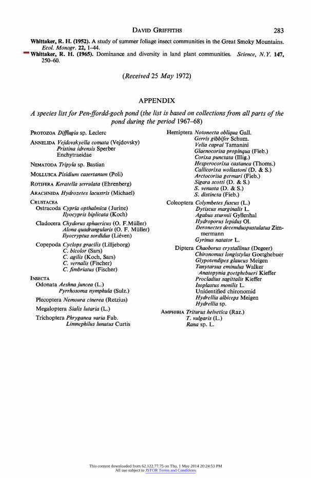
Oblique tow-net samples (using a pond net of mouth diameter 21 cm and with 24 meshes/cm) were taken on a number of occasions from the open water but very few ani- mals were ever caught (a few individuals of Chydorus), suggesting that the fauna is restricted to the vegetated areas. The species collected over a 2-year period are listed in the appendix. Compared with other upland ponds examined (Laurie 1942; Macan 1949) there are some notable absences. No leeches, hydracarine mites, gastropod molluscs, Gammarus, mayflies or fish were found. The total number of species was fifty-four, compared to the 100 and 115 found by Laurie and Macan respectively.
N
(a) 5 *
ifluyceri l flifons - Potamoqeton po/ygonifo/ius
I0 loo t |IIduncus bulbosus 1100 f
- effusus
(b)
l~~~~~~~~~Oft
FIG. 1. (a) Outline map of Pen-ffordd-goch pond and the associated streams. The vegetated areas are shaded. The region indicated by the arrow is shown in greater detail in (b).
(b) The distribution of the vegetation in the sample area.
METHODS
Samples were taken with a metal box designed to enclose a vertical column of water and the surface layer of the substratum. With this device I could take samples of plants and animals quantitatively and fairly unselectively, the animals ranging in size from ento- mostracans to full grown dragonfly larvae. Table 1 shows the densities of some of the larger animals as estimated by net sampling and by using the sampler. The agreement is reasonable in most cases.
This content downloaded from 62.122.77.75 on Thu, 1 May 2014 20:24:53 PMAll use subject to JSTOR Terms and Conditions
Table 1. The mean number of individuals of the larger species expressed per 225 cm2 (cross-sectional area of the sampler) caught by the sampler and by standard net sweeps in the two plant zones (in 1967 each standard net sweep covered an area of approximately
4500 cm2 and in 1968 6300 cm2)
Glyceria zone samples Juncus-Potamogeton zone samples Net 1967$ Net 1968 Sampler 1967 Net 1967$ Net 1968 Sampler 1967
* P<0'05 for means between plant zones (t-test). t P<0 05 for means estimates within plant zones. $ The densities of only three species were recorded in the 1967 net collections.
Samples were taken at 3-ft intervals along six lines laid down as shown in Fig. 2. Many samples were collected and those analysed were taken randomly from the ones collected in each vegetational zone (defined later). While not sampling the area in a random manner this approach was adopted for practical reasons. Samples were collected in spring and autumn. The spring samples were taken primarily to test the efficiency and ease of use of the sampler, and to develop procedures for the extraction of the animals.
On collection, the samples, consisting of a mixture of mud, plant material and animals, were preserved in Pampel's fluid, and sorted in two operations, a purely physical sorting followed by chemical separation. Each sample was washed through four filters of decreasing mesh size. The first two retained the larger animals (and some small ones) which were identified and counted, and the plant material which was classified (to species,
A B C D E
FIG. 2. The lines along which samples were taken and the positions of the samples analysed. Sampling lines A-E were 10 ft (305 m) apart.
D
This content downloaded from 62.122.77.75 on Thu, 1 May 2014 20:24:53 PMAll use subject to JSTOR Terms and Conditions
and to coarse and medium debris), dried, and weighed. The contents of the last two filters, consisting of fine debris, gravel particles and animals, were subsampled. One-quarter (excluding the gravel) was dried for 24 h at 105? C and weighed, and one-quarter used to estimate the numbers of animals. These were separated from the gravel and debris by (1) a benzene separation technique (Salt & Hollick 1944) followed by (2) sugar flotation. By this stage most species had been removed from the debris and remaining individuals, mainly oligochaetes, were estimated by further subsampling and counting.
The dry weights of animals were determined by drying individuals or groups of indi- viduals at 1050 C for 24 h. Some loss of volatile, especially lipid, constituents occurs at this temperature, but their dry weight contribution is small (Southwood 1966). The biomass of the species in each sample was calculated by multiplying the obtained dry weight by the appropriate factor.
RESULTS
The composition of the samples
The flora As mentioned earlier and illustrated in Fig. 1 there was a clear difference in the distri-
bution of the plant species; Juncus and Potamogeton were found mainly in the shallow water and Glyceria mainly in the deeper water. These two areas of vegetation will be referred to as zones. The difference between the zones was obvious to an observer but differences in the composition of the vegetation within the zones were less obvious. The percentage similarity coefficient (PSC), was used to detect differences in the composition of the plants and animals in the samples (Whittaker 1952). Values of the coefficient vary from 000, if the samples have no species in common, to 100% if the samples are identical in composition. The PSG was calculated for each pair of samples and the values entered in a trellis diagram, the samples showing the greatest similarity placed together (Macfadyen 1954). The identification of groups, which is subjective, is presented visually. In Fig. 3, for example, the arrangement of the samples has been mirrored on the other side of the diagonal, the degree of similarity between samples being indicated by the intensity of the shading.
The dry weights of plant material were used to calculate PSC values. The living plant material was divided into species, and the dead material divided on the basis of particle size. The debris retained by filter 3 was judged to be similar in appearance and compo- sition in both plant zones but that retained by filter I appeared different. However, the results are not seriously affected if the material retained by filter 1 is judged to be similar in both zones.
The results are in complete agreement with the direct observation that there are two distinct vegetational zones, the samples which form one group (D6-D3 in Fig. 3) having been collected in the Glyceria zone while the remaining samples were collected in the Juncus-Potamogeton zone. There are suggestions of two further groups within each major grouping. Thus samples D6-B7 (group 1) show some differences from samples E4-D3 (group 2) and likewise samples F7-B2 (group 3) and Cl-Dl (group 4) differ. Table 2 shows the mean percentage composition (and the corresponding standard errors) of the plants for each group of samples. There are no significant differences in the percentage composition of groups 3 and 4 but groups I and 2 differ in the percentages of Sphagnum, Glyceria, coarse and fine debris (the tests for differences between means were carried out on percentages transformed to arcsins to normalize the distributions). An explanation
This content downloaded from 62.122.77.75 on Thu, 1 May 2014 20:24:53 PMAll use subject to JSTOR Terms and Conditions
FIG. 3. Trellis diagram showing the degree of similarity between samples, based on the percentage composition of the plants in the samples. See text for further explanation.
of these differences is given later. The absence of significant differences between groups 3 and 4 is because of similarity of composition and is not due to large standard errors making distinction between the two groups difficult.
When a rank correlation between the order of samples along the side of the trellis diagram and the depth of water is calculated, a significant association is found (using Kendall's rank correlation coefficient P = 0001), i.e. the composition of the vegetation
Table 2. The mean percentage composition of the vegetation for the four groups of samples showing compositional differences in the trellis diagram
FIG. 4. Trellis diagrams showing the degree of similarity between samples, based on the percentage composition of the animals in the samples in terms of (a) numbers and (b)
biomass.
This content downloaded from 62.122.77.75 on Thu, 1 May 2014 20:24:53 PMAll use subject to JSTOR Terms and Conditions
changes with depth, group 4 samples coming from the shallowest water and group 1 from the deepest.
The fauna Trellis diagrams were also constructed using the faunal fractions of the samples. The
composition of the samples was determined using both numbers of individuals and bio- mass. By using biomass data any discontinuities in the distributions of rare but large animals such as Sialis and Pisidium can be considered. In Fig. 4 only the shaded portions of the diagrams are shown.
No division of the samples into major groups is possible and the order of samples along the sides of the diagrams also differs from that in Fig. 3. There is a general trend of decreasing similarity between samples and a just significant correlation between the order of the samples along the sides of the diagram and the depth of the water when numbers are used. Hence although the vegetation in the shallower water is more uniform in com- position the animals in this area show the greater variation in relative abundance. The absence of discontinuities between the samples collected from the two zones further suggests that the composition of the vegetation has little effect on the overall composition of the fauna. In fact some samples from the shallow water zone, e.g. D2, more closely resemble those from the Glyceria zone than do others which were collected in that zone, e.g. D3.
The distribution of individual species
A number of measures of the dispersion of individuals have been devised, Morisita's 13 index being used here (Morisita 1959). An index value of 10 is obtained when the distribution is random, a value > I 0 when it is aggregated, and a value < I 0 when the distribution is regular. The greater the deviation from I 0 the larger is the departure from a random distribution. As Baroni-Urbani (1969) has correctly pointed out it is not pos- sible to test the significance of an 13 value < I 0 using the formula provided by Morisita (though Baroni-Urbani quoted the formula incorrectly). In the few cases where 13 values smaller than unity were obtained their significance was assessed by the variance/mean ratio test.
The dispersion pattern detected by sampling depends on sample size. For practical reasons a single sampling unit was chosen. The effect of this decision on the results ob- tained will be considered in the discussion.
Dispersion patterns of the animals The Ib values for some of the more common animals have been calculated for each of
the sample groups noted earlier and for all samples combined (Table 3). With one exception all of the species have aggregated distributions. The Ib values for the group 'All samples' are generally higher than those for the separate, smaller groupings. Because of the larger area considered in the former case the environment is more likely to appear heterogeneous to a species and hence higher 16 values are to be expected. For example, the mean number of Ilyocryptus per group of samples varied from 0 to 161. The exception to these results, Sialis, is of considerable interest. The species appears randomly dispersed in the four sample groups and in three of these groups the index is below one, suggesting regular distributions. When tested by the variance/mean ratio the individuals in the group 1 samples are found to be regularly dispersed (probability of randomness 001) but the dispersion of the individuals in the group 3 and 4 samples is not significantly different
This content downloaded from 62.122.77.75 on Thu, 1 May 2014 20:24:53 PMAll use subject to JSTOR Terms and Conditions
* Not significantly different from random (P>0 05). t In this group of samples the species is regularly dispersed as assessed by the variance-
mean ratio test.
from random. Regular distributions have been infrequently demonstrated in nature among invertebrates and are usually interpreted as being indicative of competitive interactions.
The samples were divided into two, those collected in each zone, to reduce the effect of environmental heterogeneity, and 16 values recalculated. The use of zones for the calculations seems legitimate as it is a natural division to adopt. Any further subdivision, e.g. groups 1-4 described earlier would, given the small number of samples, possibly have affected the stability of the index (the index shows little variation when 8 or more
Table 4. The dispersion pattern (16) values, mean numbers and mean biomass per sample for the species collected in the Glyceria and Juncus-Potamogeton zones
Glyceria zone samples* Juncus-Potamogeton zone samples Id Mean number/ Mean biomass/ 1( Mean number/ Mean biomass/
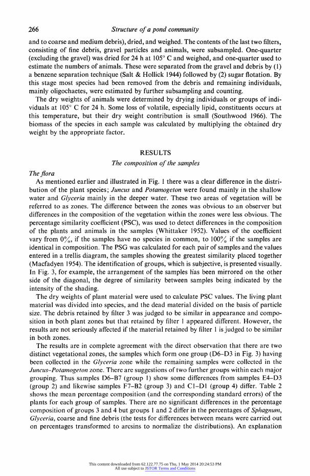
FIG. 5. The relationship between the degree of aggregation (16) and the log mean abundance (in terms of numbers and biomass respectively) of the species found in the Glyceria zone
samples (a and b) and in the Juncuts-Potamogeton zone samples (c and d).
This content downloaded from 62.122.77.75 on Thu, 1 May 2014 20:24:53 PMAll use subject to JSTOR Terms and Conditions
samples are used). Sample D3 was omitted from consideration because of the low level of similarity this sample showed with the others in terms of faunistic composition (Fig. 4). Both of the above decisions were made a priori and resulted in improved correlations.
The 13 values for the samples from the two zones are shown in Table 4 along with the mean numbers and biomass of each species in these zones. Hairston (1959) found an inverse correlation between the abundance of a species and the degree of aggregation of that species and these results agree with that finding (Fig. 5). In both zones biomass gives a better fit than numbers (also logarithmic plots of abundance give better correla- tions than linear ones). There is a better correlation between the variables in the Juncus- Potamogeton zone but in the light of the findings of the previous section it is not clear why this should be so. These results support the earlier conclusion that the dispersion patterns are mainly reflecting environmental heterogeneity with the more common animals finding more of the environment suitable for them than the rare ones (as evi- denced by their more nearly random distribution patterns).
Table 5. The mean weights, variances and variancelmean ratios of the vegetation in the plant zonest
Glyceria zone samples Juncus-Potamogeton zone samples Mean weight Variance Variance/ Mean weight Variance Variance/
* P<0.05. t A variance/mean ratio of 1 indicates a random distribution. The significance of the difference between
the ratio and 1 was assessed by the t-test.
The pond net collections of the larger animals (Table 1) show a number of significant differences in the densities of the animals in the shallow and deep water. From this table and from other collections Limnephilus, Hydroporus, and Corixa were shown to be restricted to the shallow water zone though the reasons for the restrictions are not known.
Dispersion patterns of the plants Morisita's index was unsuitable for measuring the dispersion patterns of the plant
material because of its dependence on discrete variables, while only weight estimates were available for the plants. Instead the variance/mean ratio test was used (Table 5). Most of the plant material was randomly distributed, the one exception, the fine debris in the shallow water, being aggregated.
Associations between species
Kendall's rank correlation coefficient was used to calculate the degree of association between variables, i.e. the weights of plant material and the numbers of animals. This coefficient considers only the rank, i.e. the order, of a set of measurements and makes no assumptions as to.the distribution of the variables. Kendall (1962) shows how to calculate
This content downloaded from 62.122.77.75 on Thu, 1 May 2014 20:24:53 PMAll use subject to JSTOR Terms and Conditions
the coefficient tau. The results, however, are not expressed in terms of tau but of S where, in the absence of tied rankings,
2S tau =
n(n - 1)
The maximum value of S, i.e. a perfect correlation, is given by n(n-1)/2 where n is the number of samples. In the following section the correlations are expressed in terms of the statistic S primarily because the level of significance of the correlation is determined solely by S and the value of tau largely by S.
Correlations between organisms in the Glyceria zone are dealt with first and then the procedure repeated for the Juncus-Potamogeton zone.
Glyceria zone Values of S for the plant material are given in Table 6. About 90%0 of the plant material
in the samples is debris (see Table 2), and this has arisen from the Glyceria and Sphagnum,
Table 6. Associations (as measured by the statistic S) between the plants and plant materialfound in the Glyceria zone samples
u u , , U | E :
22* 9 22* 6 -2 8 Sphagnum 8 23* -3 -15 8 Glyceria
10 0 0 6 Juncus 11 3 27* Coarse debris
32* 29* Medium debris 21* Fine debris
Coarse and medium debris
Smax = 5
* Correlation significant at 500
level.
Juncus bulbosus forming a very small percentage of the plant material. There are significant positive correlations between the amounts of Glyceria and Sphagnum and the amount of coarse debris, and an almost significant negative correlation between the weight of Gly- ceria and the weight of fine debris. These associations probably reflect the pattern of breakdown of the two species. The coarse debris can be regarded as the first stage in the decay of dead vegetation and hence would be expected to be found adjacent to the living plants (as supported by the significant positive correlation between the two). As time passes the debris becomes more finely broken up and is found principally between indi- vidual plants.
At this point it is of interest to return to the differences noted between the samples forming groups 1 and 2 (Table 2). The Glyceria appeared denser in the deeper water (from which the group 1 samples were collected) and hence group 1 samples are more likely to have enclosed individual plants and group 2 samples to have been taken between plants. This would explain why group 1 samples had significantly more Glyceria, Sphagnum and coarse debris and significantly less fine debris than group 2 samples.
This content downloaded from 62.122.77.75 on Thu, 1 May 2014 20:24:53 PMAll use subject to JSTOR Terms and Conditions
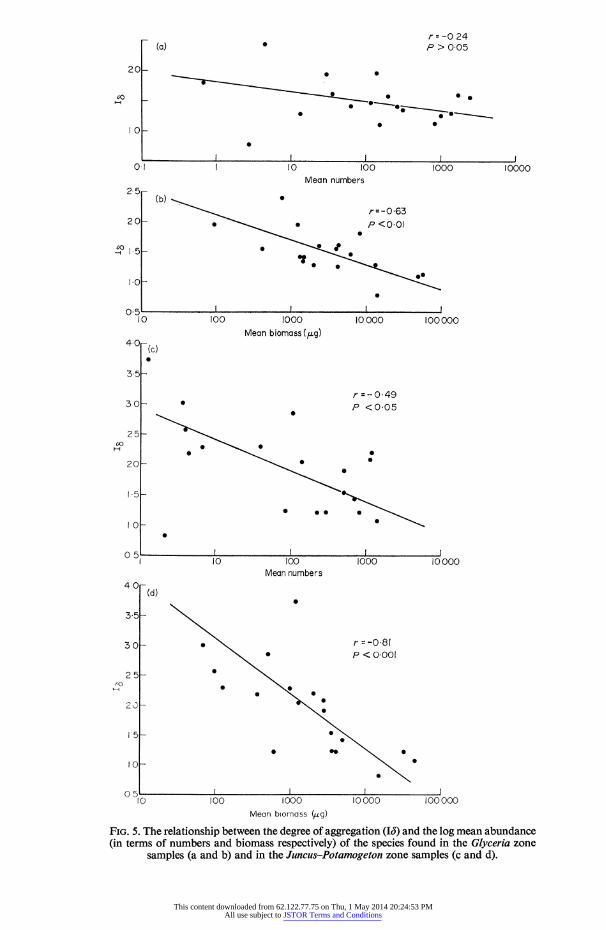
There are few significant correlations between the numbers of each animal species and the weights of plant material but the figures do show interesting trends (Table 7). For example, the numbers of Hydrozetes were correlated with the weight of Glyceria and to a lesser extent with the weight of Sphagnum (the animals were observed crawling over the Glyceria). Bearing in mind the general plan of the vegetation one sees that as the distance from the Glyceria plants increases then the correlations decrease; negative associations were noted between Hydrozetes and the two finest grades of debris. One can therefore use both the significant correlations and the observed trends in the coefficient to deter- mine the location of different species, though clearly the use of trends results in only a very approximate localization.
Table 7. Associations (as measured by the statistic S) between the animals and plants found in the Glyceria zone samples
The majority of the twenty-one species investigated showed some degree of association with the Glyceria and/or Sphagnum. The reverse trend was much less common and only one species, the tube dwelling chironomid larva Chironomus, showed any tendency to- wards living in the fine debris. Chydorus, Ilyocryptus, and Cyclops gracilis were associated with the depth of water rather than with any other factor while some species showed no positive trends.
Values of the coefficient between animal species were also calculated and these values entered into a trellis diagram. The animals formed three rather indistinct groups (Table 8), i.e. it was not possible in some instances to tell if a species belonged to one or other of of the groups. Two groups, found at the ends of the diagonal, are characterized by positive
This content downloaded from 62.122.77.75 on Thu, 1 May 2014 20:24:53 PMAll use subject to JSTOR Terms and Conditions
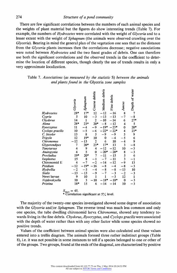
Table 9. Associations (as measured by the statistic S) between the plants and plant materialfound in the Juncus-Potamogeton zone samples
q
10 9 -11 19* 19* Sphagnum -2 -12 2 -2 Glyceria
0 16* 15* Juncus -8 -6 Potamogeton
24* Medium debris Fine debris
* mCorrelation significant at 5% level.
correlations while the third shows mainly negative ones. One of the positive correlation groups is composed of species which were found on or about the Glyceria plants while the other is composed of species observed to be living around the vegetation on the mud surface. The third group consists of species found mainly in between individual plants, associated with the fine debris. Hence these results parallel those obtained above. For example, both Alona and Procladius are significantly associated with the GlIyceria and also show a significant positive correlation with each other.
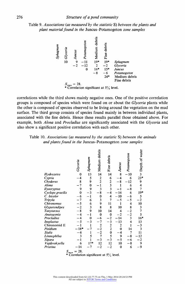
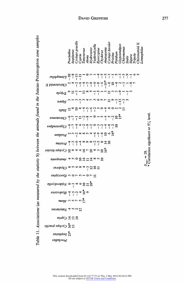
Table 10. Associations (as measured by the statistic S) between the animals and plants found in the Juncus-Potamogeton zone samples
Juncus-Potamogeton zone The procedure was repeated for the samples from the shallow water zone. Correlations
between plants are listed in Table 9. The arrangement differs from that noted in the Gly- ceria zone, there being no indication of the pattern of breakdown noted for that zone. Correlations between plants and animals are shown in Table 10. There are few significant correlations and again trends in the degree of association can be seen. The results are even less decisive than those from the Glyceria zone but the majority of species are associated with the Spagnum, medium debris, fine debris, Juncus complex. Coupled with a large number of negative associations with the sparse Glyceria this suggests that the complex is fulfilling a similar role to that played by the Glyceria in the deep water zone, i.e. the vegetation is functioning as a substratum. Again the correlations between animals (Table 11) parallel the results obtained between animals and plants.
DISCUSSION
Species distributions
The dispersion pattern of a species is affected by a number of factors listed as follows. (a) It has already been shown that commonness implies a less aggregated dispersion
pattern than rareness. (b) Elton (1966) has suggested that an inverse pyramid of habitats exists, i.e. that herbi-
vores are more or less restricted to the vicinity of their food plants while carnivores will be found feeding over a wider area. Tilly (1968) found some evidence for a similar proposal and suggested that carnivores need to be more evenly spaced to reduce the possibility of cannibalism. The results from the Glyceria zone neither confirm or contra- dict these suggestions. However, comparison of the regression lines of the carnivores and the detritus feeders/herbivores from the Juncus-Potamogeton zone showed that, although the slopes of both lines were similar, that of the carnivores was below that of the detritus feeders (although not significantly different from it), i.e. there was a tendency for the carnivores to be more regularly dispersed.
(c) Individuals of a species are often responsive to the presence of adjacent individuals and adjust their relative positions accordingly. The regular distributions of many species of bird pairs during the breeding season is a well-known example and Sialis in group 1 samples seems likely to be a further instance.
The large cross-sectional area of the sampler resulted in a type (a/b) pattern (above) being detected in the majority of cases. It seems likely that a type (c) pattern will be found if the mean number of individuals per sample is in the range 1-5. For most species sampling on such a small scale is not possible.
The data of Table 7 were examined for evidence of differences in the horizontal dis- tributions of ecologically closed related species, i.e. possible competitors. Of the three cladoceran species only one, Alona, showed a significant association with the vegetation, while the other two species were separated vertically, Ilyocryptus living at the mud surface and Chydorus living in the open water near the Glyceria leaves. Differences can also be seen in the distributions of the copepods, chironomids, and annelids. Values of the correlation coefficient between possible competitors were mostly small and in no instances were large negative correlations found, i.e. evidence of species exclusion.
Species abundances A number of authors have derived models to predict the relative abundances of species
This content downloaded from 62.122.77.75 on Thu, 1 May 2014 20:24:53 PMAll use subject to JSTOR Terms and Conditions
I I I I I III I I I I I I I I 4 8 12 16 20 24 28 32
Ranked sPecles abundances FIG. 6. Importance value curves for the animals collected in the pond. (a) Importance values expressed in terms of numbers. The line was fitted from the geometric series. (b) Im- portance values expressed in terms of biomasses. The lines represent the geometric series
(A), the lognormal distribution (B), and the MacArthur broken stick model (C).
+2 _
100 -~~~~~~~~~~~~~~~
1 10 100 1000 10000 100000
E~~~~~~~~~ 0-10~~~~~~~
cr~~~~~~
0
Mean body dry weights (,ug)
FIG. 7. A rankit test for lognormality in the distribution of dry body weights of animals from the pond (the line was fitted by eye).
This content downloaded from 62.122.77.75 on Thu, 1 May 2014 20:24:53 PMAll use subject to JSTOR Terms and Conditions
in a community. Whittaker (1965) represented these models on importance value curves, importance values being measured in numbers, biomass, etc., and being plotted on a logarithmic scale against rank. In Fig. 6(a) importance is measured in numbers. The points clearly fall along a straight line, i.e. the abundances are described by a geometric series. The results are replotted in Fig. 6(b) in terms of biomasses (the loss of two species is because no biomass data were available for these species). Three lines are shown, generated by the geometric series (A), the lognormal distribution (B), and the Mac- Arthur broken stick model (C). The second of these models best describes the data. The biomass data are the numerical data multiplied by the mean size of each species. Hence the change from a geometric series to an approximately lognormal distribution must be a reflection of the size distribution of the species. In Fig. 7 the logarithms of species mean body weights (as a measure of size) are plotted in a rankit diagram as a test for lognormality (Bliss 1967). Most of the points fall along a straight line (fitted by eye), approximating a lognormal size distribution. The departure of the smaller species from the line indicates skewness, a feature also found by Hemmingsen (1934) and Schoener & Janzen (1968) in their studies on body size. Whittaker examined a number of plant communities and found that the three models applied in different situations. The geo- metric series best fitted communities from severe environments and with few species while the lognormal was more characteristic of rich communities, i.e. those with many species. If similar generalizations are to be looked for in animal assemblages it is neces- sary to use just one measure of importance as Whittaker did since, as shown above, different measures from one community fit different models. Numerical data seem to provide the best measure. Consider two communities, one of which is best described by the geometric series and the other by the lognormal distribution when numerical data are used. If the weights of species comprising communities are lognormally distributed then, when one considers biomass data, both communities will be described by the log- normal distribution, i.e. the product of a lognormal distribution and a geometric series is a lognormal distribution (see above) and the product of two lognormal distributions is also a lognormal distribution. From a knowledge of the location of the pond one would expect the geometric series to be the most appropriate if the generalization were true.
The numbers of individuals found have thus far been expressed in terms of sample units. Converting these to numbers/M2 (by multiplying by 44.4) gives an average value of 338 000. This value is considerably higher than any other published figure for the numbers of benthic animals, most falling in the range 1000-20 000 individuals per square metre. Omitting Chydorus and Cyclops gracilis, which are perhaps not truly benthic, only reduces the figure to 190 000/M2. These high numbers can be partly explained by the relatively high efficiency of the sampling and sorting techniques.
Detritus and the functioning of the community
Darnell (1964), Minshall (1967), Carlson (1968), and Tilly (1968) have demonstrated the importance of detritus in a variety of aquatic ecosystems. This study also indicates the considerable role played by detritus in the functioning of the community. In the spring collection 67.5% of the animals were found to be feeding on detritus and only 900 on plants (900 could not be assigned to any trophic level because of lack of data) while in October 88% were feeding principally on detritus, the only animal shown to be entirely herbivorous being Limnephilus. The Hydrellia larvae, however, are probably herbivores. The detritus feeders comprised 7300 of the total standing crop in terms of dry weight with the exclusively detritus-feeding Pisidium, Pristina, and Vejdovskyella
This content downloaded from 62.122.77.75 on Thu, 1 May 2014 20:24:53 PMAll use subject to JSTOR Terms and Conditions
comprising 65% of the standing crop. These three species probably play a major rOle in community metabolism and their ecology differs from that of the other species found in the pond. Both Pisidium and Pristina in the shallow water and Pisidium in the deeper water were found mainly between the clumps of vegetation, associated with the fine debris. Since most species were associated with the vegetation this helps to explain the apparently low predation levels to which these detritivores were subject. Pisidium, for example, was found only in the guts of newt larvae in April while the oligochaetes were eaten by several predator species though Sialis was the only major one at the times investigated. Sialis was also found between the vegetation, further indicating the relative isolation of a major trophic pathway. In contrast Egglishaw (1964) showed that about 7000 of the species in the stream he studied were associated with the detritus, though in this instance no higher plants were present.
The detritus in the pond is probably autochthonous in origin (I discovered no terres- trial vegetation in my samples) and probably comes largely from the breakdown of the Glyceria plants (though epiphytic algae could also be important). Of the macrophytic vegetation only Sphagnum was eaten and then only by a few uncommon species. Hence the vegetation in Pen-ffordd-goch pond can be seen to have two major roles. It functions as a source of detritus, apparently the most important community food, and it also acts as a substratum for the majority of the animals. Considering this the absence of any sharp faunal changes associated with the vegetational discontinuities is easily understood. Gajevskaja (1958, 1969) has considered the importance of macrophytic vegetation as a food source in freshwater habitats. In her 1958 paper she concluded that it was of little direct importance, this frequently being due to the presence of protective devices, e.g. hard siliceous coverings. However, in her more recent publication, based on a compre- hensive survey of the literature, she concludes that rooted vegetation is eaten by many animals and is an important direct source of food in many aquatic habitats. A number of authors have found no evidence of vegetation acting as a major direct food source and the sharp disagreement over the importance of macrophytic vegetation suggests a real difference between aquatic habitats in the role played by these plants.
ACKNOWLEDGMENTS
I wish to thank Professor J. Brough for provision of facilities in the Department and Dr B. W. Staddon for help and encouragement throughout the investigation. I am grateful to Dr Staddon and Dr H. S. Horn for many helpful comments on the manuscript. The following were kind enough to provide taxonomic assistance: B. H. Cogan, J. W. Coles, S. P. Dance, J. R. Etherington, P. Freeman, A. M. Hutson, D. Macfarlane, K. G. McKen- zie, R. W. Sims, and P. F. Williams. This work was carried out whilst in receipt of a S.R.C. research studentship, and was part of a Ph.D. research project.
SUMMARY
(1) The spatial relations of the plants and animals comprising an acid moorland pond community were investigated.
(2) Of the plant species Juncus and Potamogeton were found in the shallow water and Glyceria in the deeper water.
(3) There was no obvious difference in the fauna of the two zones and no sharp change in faunal composition corresponding with the floral change.
E
This content downloaded from 62.122.77.75 on Thu, 1 May 2014 20:24:53 PMAll use subject to JSTOR Terms and Conditions
(4) All the animals, except Sialis, had aggregated distributions. This was due to environmental heterogeneity, some areas being more suitable for a species than others.
(5) An inverse relationship between the abundances of the animals (in terms of bio- mass) and the degree of aggregation was demonstrated for the animals from each zone.
(6) The associations between plants, plants and animals, and between animals were measured by a rank correlation coefficient. In the Glyceria zone the majority of the ani- mals were associated with the plants.
(7) In the Juncus-Potamogeton zone the majority of the animals were associated with the Sphagnum/debris/Juncus complex.
(8) Species abundances are compared with various models, the best fit being given by the geometric series. The species size distribution is approximately lognormal.
(9) The majority of the animals in the pond were feeding on detritus, very little living vegetation being eaten.
(10) The rooted vegetation is probably the major source of detritus in the community.
REFERENCES
Baroni-Urbani, C. (1969). Ant communities of the high-altitude Appennine grasslands. Ecology, 50, 488-92.
Berg, K. (1938). Studies on the bottom animals of Esrom Lake. K. danske Vidensk. Selsk. Skr., Ser. 9, 8, 1-255.
Bliss, C. I. (1967). Statistics in Biology, Vol. 1. McGraw-Hill, New York. Carlson, C. A. (1968). Summer bottom fauna of the Mississippi River, above dam 19, Keokuk, Iowa.
Ecology, 49, 162-9. Darnell, R. M. (1964). Organic detritus in relation to secondary production in aquatic communities.
Verh. int. Verein. theor. angew. Limnol. 15, 462-70. Elton, C. S. (1966). The Pattern of Animal Communities. Methuen, London. Egglishaw, H. J. (1964). The distributional relationship between the bottom fauna and plant detritus in
streams. J. Anim. Ecol. 33, 463-76. Gajevskaja, N. S. (1958). Le role de groupes principaux de la flore aquatique dans les cycles trophiques
des differents bassins d'eau douce. Verh. int. Verein. theor. angew. Limnol. 13, 350-62. Gajevskaja, N. S. (1969). The Role of Higher Aquatic Plants in the Nutrition of the Animals of Fresh-water
Basins. (Translated from the Russian by D. G. Maitland Muller). Boston Spa. Griffiths, D. (1973). The food of animals in an acid moorland pond. J. Anim. Ecol. 42, 285-93. Hairston, N. G. (1959). Species abundance and community organization. Ecology, 40, 404-16. Hemmingsen, A. M. (1934). A statistical analysis of the differences in body size of related species.
Vidensk. Meddr dansk naturh. Foren. 98, 125-60. Kendall, M. G. (1962). Rank Correlation Methods, 3rd end. Griffin, London. Laurie, E. M. 0. (1942). The fauna of an upland pond and its inflowing stream at Ystumtuen, North
Cardiganshire, Wales. J. Anim. Ecol. 11, 165-81. Macan, T. T. (1949). Survey of a moorland fishpond. J. Anim. Ecol. 18, 160-86. Macfadyen, A. (1954). The invertebrate fauna of Jan Mayen Island (East Greenland). J. Anim. Ecol.
23, 261-97. Minshall, G. W. (1967). Role of allochthonous detritus in the trophic structure of a woodland springbrook
community. Ecology, 48, 139-49. Morisita, M. (1959). Measuring of the dispersion of individuals and analysis of the distributional patterns.
Mem. Fac. Sci. Kyushu Univ. Ser. E (Biol.), 2, 215-35. Odum, H. T. (1957). Trophic structure and productivity of Silver Springs, Florida. Ecol. Monogr. 27,
55-112. Salt, G. & Hollick, F. S. J. (1944). Studies of wireworm populations. 1. A census of wireworms in pasture.
Ann. appl. Biol. 31, 52-64. Schoener, T. W. & Janzen, D. H. (1968). Notes on environmental determinants of tropical versus tem-
perate insect size patterns. Am. Nat. 102, 207-24. Sjors, H. (1950). On the relation between vegetation and electrolytes in North Swedish mire waters.
Oikos, 2, 241-58. Southwood, T. R. E. (1966). Ecological Methods, with Special Reference to the Study of Insect Populations.
Methuen, London. Tilly, L. J. (1968). The structure and dynamics of Cone Spring. Ecol. Monogr. 38, 169-97.
This content downloaded from 62.122.77.75 on Thu, 1 May 2014 20:24:53 PMAll use subject to JSTOR Terms and Conditions
Copepoda Cyclops gracilis (Lilljeborg) C. bicolor (Sars) C. agilis (Koch, Sars) C. vernalis (Fischer) C. fimbriatus (Fischer)
INSECTA Odonata Aeshnajuncea (L.)
Pyrrhosoma nymphula (Sulz.)
Plecoptera Nemoura cinerea (Retzius)
Megaloptera Sialis lutaria (L.)
Trichoptera Phryganea varia Fab. Limnephilus lunatus Curtis
Hemiptera Notonecta obliqua Gall. Gerris gibbifer Schum. Velia caprai Tamanini Glaenocorisa propinqua (Fieb.) Corixa punctata (Illig.) Hesperocorixa castanea (Thoms.) Callicorixa wollastoni (D. & S.) Arctocorisa germari (Fieb.) Sigara scotti (D. & S.) S. venusta (D. & S.) S. distincta (Fieb.)