THE STRUCTURE OF INDIRECT TAXATION AND ECONOMIC...

Journal of Public Economics 1 (1972) 97-l 19.0 North-Holland Publishing Company

THE STRUCTURE OF INDIRECT TAXATION

AND ECONOMIC EFFICIENCY *

A.B. ATKINSON and J.E. STIGLITZ

University of Essex, Colchester, England and Yale University, New Haven, U.S.A.

First version received October 197 1, revised version received November 197 1

The recent literature on indirect taxation has been characterised by

two disjoint strands. On the one hand, there are the advocates of the

replacement of differentiated indirect taxes by a uniform tax on all

commodities (such as a value added tax). Their case is based in part on

administrative simplicity, but rests largely on the belief that a uniform

tax is more conducive to economic efficiency. On the other hand, there

is the literature on “optimal commodity taxation” arguing that dif-

ferent commodities ought to be taxed at different rates, since this re-

duces the dead weight loss. This line of argument, which was first put

forward by Ramsey (1927) and later extended by Samuelson (195 l),

has been the subject of a number of recent papers. ’ Although both ad-

vocates and critics of differentiated indirect taxes have been primarily

concerned with economic efficiency, the debate has never really been

joined: each side has discussed the issue as though the other did not

exist. The results of Ramsey have been ignored or dismissed as being of

little practical significance (cf. Prest, 1967 and Musgrave, 1959). On the

other hand, the recent studies in optimal taxation have made little at-

* The authors are grateful to J.A.Mirrlees for his very helpful comments on an earlier version

of this paper. It has also benefitted a great deal from comments made at seminars at the univer-

sities of Essex, Kent, Southampton, York, University College, London and Nuffield College, Oxford. Stiglitz’s research was supported under grants from the Ford Foundation and the Na-

tional Science Foundation. * The revival of interest in this area owes much to the paper by Diamond and Mirrlees

(1971); see also Stiglitz and Dasgupta (1971), Dixit (1970) and Lerner (1970).

98 A.B. .4 tkinson, J.E. Stiglitz, Indirect taxatiorz and economic efficiency

tempt to relate their findings to the conventional views - to show to

what extent they are simply alternative forms of conventional maxims

for the design of the tax system and to what extent they are in fact con-

tradictory.

The purpose of this paper is to present a new formulation of the op-

timal tax problem which gives more insight into the structure of the so-

lution and provides more easily interpreted results. Using this formula-

tion, we try to clarify the relationship between the results on optimal

taxation and the conventional wisdom, making clear where and under

what conditions they are in agreement. Moreover, using this new ap-

proach it is possible to calculate the optimal tax structure corresponding

to empirically estimated demand function, and some numerical results

are presented.

1. The conventional wisdom

A number of criteria for evaluating alternative tax structures have

been proposed: (a) efficiency; (b) equity; (c) administrative simplicity;

(d) flexibility (usefulness for stabilization policies). This paper focuses

primarily on the first of these considerations, since it is the efficiency

aspects that have received most attention. The analysis does, however,

have important implications for the conflict between efficiency and

equity and these are discussed briefly in the final section. (In a sequel

to this paper, the distributional arguments and the relationship between

direct and indirect taxation are examined in more detail.) The last two

considerations - administrative simplicity and flexibility - are not dis-

cussed, but it should be emphasised that this does not imply that in our

judgment these other effects are not of importance. Against any gains

from differentiation on the first two accounts must be set some judg-

ment of the political ’ and economic benefits to be had from the sim-

pler administrative structure associated with uniform taxes.

’ In particular, once the principle of differentiation is accepted, the tax system may be sub- jected to the pressures of special interest groups; each group would argue that special conside-

rations dictate that the tax on its commodity (its factor use) be lowered. The tax structure even-

tually emerging might well be based as much on relative strengths of these-pressure groups as on

relative dead weight losses.

A.B. Atkinson, J.E. Stiglitz, Indirect taxation and economic efficiency 99

Price to the consumer

I \ ,

Ax Quanti tY

Fig. 1.

The conventional analysis of the efficiency arguments presented in

most textbooks is based on a partial equilibrium model of a single mar-

ket (see fig. 1). As a result of the tax at rate t, the supply curve shifts

up from SS to S’S’. The tax revenue is AP’CB. The excess loss of con-

sumer surplus is PP’F and of producer surplus is PCF. The total dead-

weight loss for a given revenue (R) may be approximated for small

taxes by (see Bishop, 1968, p. 211)

R2

2qx (; + t) ’

where ed and E, denote the elasticities of demand and supply, and qx

denotes expenditure on the commodity. From this are derived the fol-

lowing maxims: to minimise distortion we should tax those goods which

100 A.B. Atkinson, J.E. Stiglitz, Indirect taxation and economic efficiency

(i) have a low price elasticity of demand, (ii) have a low price elasticity

of supply, (iii) form an important part of people’s budgets. 3 This geometric analysis gives somewhat similar results to those reach-

ed by Ramsey in one of the special cases he considered. The relation-

ship between them has, however, been obscured by the confusion in

much of the literature of two different questions:

(a) If taxes can only be imposed on one commodity (or a subset of com-

modities), which should be chosen? This is in effect the question con-

sidered by Hicks.

(b) If there is more than one taxable commodity, what should be the

relative tax rates on different commodities? This is the question con-

sidered by Ramsey.

In the former case, we wish to tax the commodity for which the dead

weight loss is lowest for a given revenue, and here maxims (i)-(iii) apply.

In the Ramsey case, we wish to minimize the total dead weight loss over

all taxable commodities, so that for each commodity the marginal dead

weight loss associated with raising a marginal dollar of tax revenue must

be the same. In the case of a perfectly elastic supply this requires (for

small taxes)

‘i -E’d = constant for all commodities i = 1, . . . . n , 4i

or that the (advalorem) tax rates be inversely proportional to the elasti-

city of demand in each industry. (Note that in this case the importance

of the good in consumers’ budgets is not relevant.) It is on the Ram-

sey question that we focus in this paper.

This partial equilibrium analysis is clearly unsatisfactory in view of

3 The following passage from Hicks (1968) perhaps comes closest to giving a fair representation of the conventional wisdom: “for a given revenue the loss of surplus will be larger, the

larger is the elasticity of demand or supply; if either is completely inelastic the loss of surplus falls to zero, and there is no tendency to substitute any other good for the taxed commodity,

the outlay tax becomes equivalent to a lump sum taken from the taxpayer . . . in all ordinary cir- cumstances, however, there will be some loss of surplus. This loss will also vary (this time inversely) with the amount spent on the article, i.e. its importance in consumption. For to raise a

given revenue from an “unimportant” commodity, very high rates of tax may be required; with

any normal elasticity of demand or supply the loss of surplus will be severe” (p. 149).


the restrictive assumptions on which it is based. In particular, it requires

(a) the absence of income effects, and (b) the independence of demand

functions. There has therefore been considerable scepticism about its

applicability. Prest (1967), for example, dismisses the Ramsey results

with the comment that “such restrictive assumptions have to be made

in order to derive a solution, that they appear to have little practical

significance” (although he offers nothing in its place). In contrast to

the restrictive partial equilibrium analysis, the results of Ramsey, Sa-

muelson, Boiteux (1951) (and more recently Diamond and Mirrlees) are

in many respects more general. In particular, they have led to the im-

portant finding that the optimal tax structure requires that (for infinite-

simal taxes) the compensated demand for each good be reduced by the

same proportion. 4 However, while this provides considerable insight

into the form of the solution, it does not yield any simple qualitative

propositions about the optimal tax structure. It does not, for example,

suggest which goods should be taxed more heavily - or indeed whether

a differentiated tax structure is in fact optimal. Moreover, it does not

readily permit the calculation of optimal rates of taxation on the basis

of empirically estimated demand functions.

The aim of this paper is to derive results midway in generality be-

tween those obtained from partial equilibrium analysis and the Ramsey-

Samuelson results. The results we derive allow straightforward state-

ments to be made in the case where all consumers are identical about

the effect of efficiency considerations on the structure of indirect taxa-

tion and facilitate the estimation of the optimal tax structure. The basic

model is described in the next section; the central results are set out in

section 3; and the implications are discussed in the remainder of the

paper.

2. The model

2.1. Assumptions about production In this paper we focus on the role of demand factors in determining

the optimal structure of indirect taxation, and therefore make the sim-

4 From what it would have been had producer prices been charged. This result is still de- pendent on certain restrictive assumptions: e.g. constant returns to scale in the private sector.


plest possible assumptions about production. Most importantly, we as-

sume constant returns to scale, which precludes any discussion of the

role of supply elasticities. ’ For ease of exposition, it is also assumed

that producer prices are fixed for all commodities and labour (the only

factor supplied by households), although the results in no way depend

on this assumption. Writing qi for the consumer price of good i, pi for

the producer price, we have qi = pi + ti. 6 We assume without 10~s of ge-

nerality that one good (leisure) is not taxed and that the wage is unity.

2.2. Assumptions about consumption A consumer is assumed to maximise a function U(x, L) subject to the

budget constraint

n

C qiXi = L ) i= 1

(2.1)

where L is the amount of labour supplied and Xi is the amount of the

consumption good purchased. Writing CY for the marginal utility of in-

come, this gives the first-order conditions

Ui = (Y qi i= 1, . . . . n (2.2a)

-uL =a. (2.2b)

2.3. Social welfare function The general assumption made is that the government maximises

a social welfare function which is individualistic and impersonal:

W[iY, uz, u3, . ..) Urn ] where Uk is the utility of the kth man. How-

ever, in order to focus on the efficiency aspects, we assume here that all consumers are identical, which means that we can consider the welfare

of a ‘representative’ individual:

U(x, L) .

’ For a discussion of the role of supply considerations, see Stiglitz and Dasgupta (1971) 6 We shall assume that these producer prices correctly reflect social costs, i.e. there are no

externalities or “imperfections of competition”.

A.B. Atkinson, J.E. Stiglitz, Indirect taxation and economic e,fficiency 103

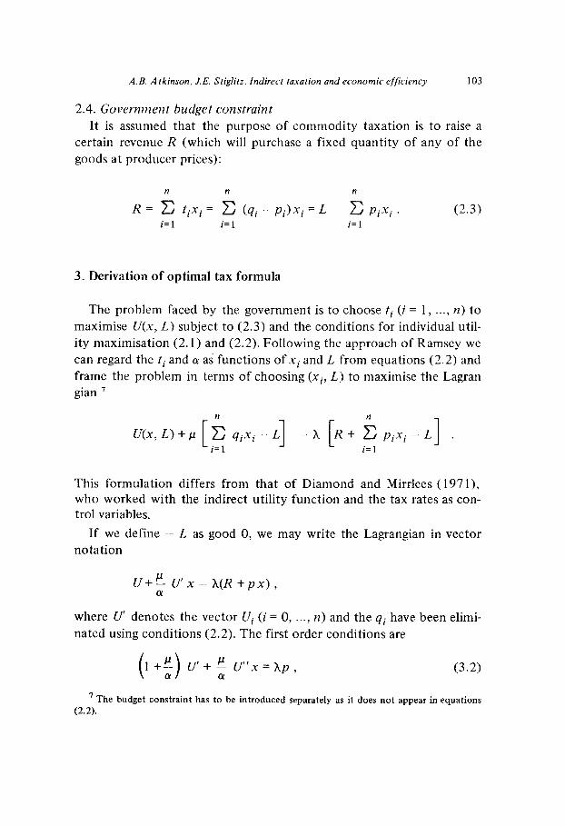
2.4. Government budget constraint

It is assumed that the purpose of commodity taxation is to raise a

certain revenue R (which will purchase a fixed quantity of any of the

goods at producer prices):

n n n

R = C tiXi = C (qi - pi)Xi = L - C PiXi .

i=l i=l i=l

(2.3)

3. Derivation of optimal tax formula

The problem faced by the government is to choose ti (i = 1, . . . . n) to

maximise U(x, L) subject to (2.3) and the conditions for individual util-

ity maximisation (2.1) and (2.2). Following the approach of Ramsey we

can regard the ti and CY as functions of xi and L from equations (2.2) and

frame the problem in terms of choosing (Xi, L) to maximise the Lagran gian I

U(X, L)+P C qixi- L [ i:, ] -x [R+ iPixihL] ’

This formulation differs from that of Diamond and Mirrlees (197 l), who worked with the indirect utility function and the tax rates as con- trol variables.

If we define - L as good 0, we may write the Lagrangian in vector

notation

U+b U’x-X(R+px),

where U’ denotes the vector Ui (i = 0, . . . . n) and the qi have been elimi-

nated using conditions (2.2). The first order conditions are

(3.2)

7 The budget constraint has to be introduced separately as it does not appear in equations (2.2).


where U” denotes the matrix Uii (i, j = 0, . . . . n). Let us define

n (- uik>xi Hk= c

i=O ‘k ’

i.e. Hk is the sum of the elasticities of the marginal utility of xk with

respect to each of the commodities. Then the first-order condition can

be written as

4k[“+/-dl -Hk)l =A& k = 0, . . . . n . (3.3)

But from the normalisation to = 0,

X-a P= ___

l-He (3.4)

so that the optimal tax rates tz as :I percentage of consumer prices are

characterised by ’

t* k _ X-cx Hk-@

Pk +$ x 1-e * (3.5)

While this equation does not in general provide an explicit formula for

the optimal tax rate (since the Hk depend on the tax rates), it does al-

low us to draw a number of conclusions about the optimal structure of

taxation. The implications of equation (3.5) will be the subject of the

remainder of the paper. 9

8 It can be seen that the assumption of fixed producer prices does not affect this result: if the government revenue constraint were replaced by a production constraint F(x) = 0, the analysis would go through as before with Fi replacing pi. Since Fi is homogeneous of degree zero, equation (3.2) is unaffected.

9 Equation (3.5) can also be obtained from the results of Samuelson, Diamond and Mirrlees by inverting their formulae (see the appendix).


4. Implications of basic optimal tax formula - uniform taxation?

One of the main questions of policy importance is whether or not a

uniform structure of taxation would be desirable. I0 From equation

(3.5) we can determine the conditions under which efficiency conside-

rations would require a uniform tax. It is in fact immediately clear that

a suflicient condition for t* - t* k - ,. all k, j 2 1 is that the indifference map

be homothetic; i.e. all the indifference curves are identical in shape; they

are simply radial “blow-ups” of any given indifference curve. To see

this, observe that if the indifference map is homothetic, there exists a

representation of the indifference map which is homogeneous of degree

one in all arguments together. Thus Ui is homogeneous of degree zero,

i.e. Ci uikxi = 0 = Hk all k.

Homotheticity of the entire indifference map is not, however, neces-

sary for the optimal tax to be uniform. Let us consider first the case

where the marginal utility of leisure is independent of the consumption

of every commodity. Then t$ = t,? all k, j 2 1 implies either -H’o = 00 or

that Hk = Hi. The first condition means that

or that the elasticity of marginal utility of labour is infinite, which im-

plies a completely inelastic supply of labour. The implications of the

second condition can be seen as follows: differentiate the first order

conditions and budget constraint (2.1) and (2.2), to obtain

-u,, u,, . . . -41

u21 u,, . . . 32

I-41 -q2 . . . 0

%

dx2

da

0

0

=

-dE

lo From this point we set pi = 1 alJ i (without loss of generality), so that uniform taxation implies fi = y, k, j > 1.


n -ukiXi

where E = c qiXi = total expenditure; defining Hki = ___ uk

we obtain i=l

(by appropriate normalisation)

H,, H,, . . . 1

H21 H,, . . . 1 (4.1)

-41x1 q2x2... 0 1

Denote by D the determinant of the matrix of coefficients of the left

hand side of (4.1). Then,

0 42 H,, . . . 1 H,, 0 H,, . . . 1

0 H22 H,, - . . . 1 H,, 0 H,, . . . 1

1 q2x.2 : . . . 0 qlxl 1 : . . . 0

= (-1)”

(I

- (-1)”

= (-1)”

H,, H,, . . . 1

H22 H23 ... 1 + Hz, H23 . . . 1

. . . . . . . . . .

H,, + H,, H,, . . . 1

Hz2 + H2r Hz3 . . . 1

Ht2 + HII Hts ..* CiHri 1 = 0,

Hz2 + H2r Hz3 ... ;I;iH,i 1

(since Hk = ~:Hki), i.e. we require equal, and hence unitary, expenditure elasticities of all commodities. If U, # 0 for some i, then ti may equal

ti even without unitary expenditure elasticities. The effects of the in-


teractions among the commodities directly may just be offset by the

interactions between the commodities and leisure. (This is illustrated in

a three commodity example given in section 8.)

In this section we have examined the conditions under which the op-

timal tax structure will be uniform. It is clear that there is no presump-

tion that these conditions are likely to obtain and in the following sec-

tions we examine how the optimal tax rates depend on the characteris-

tics of different commodities.

5. Implications of optimal tax formula - two polar cases

We now show how the results of Ramsey and others can be obtained

as polar cases of formula (3.5). Assume first that there is constant mar-

ginal disutility of labour. Then f’@ = 0 and the optimal tax is given by

t* k x-a ----z -- 1+t/$ x

Hk . (5.1)

If in addition we assume that Uii = 0 (i # i), we can see that Hk is inver-

sely proportional to the elasticity of demand. *l We have, therefore, ob-

tained the Ramsey result that the optimal taxes should be inversely pro-

portional to the price elasticity of demand.

On the other hand, if we suppose that (-Ho) tends to infinity, which

corresponds to the case of a completely inelastic supply of labour, then

$/cl + t,$) __~ =

Hk/(-@) + 1 ~ 1 ____

t:/(l + t$> HI/(-@) + 1 ’

i.e. uniform rate of tax on all goods. Since a uniform rate of tax on all

goods is equivalent to a tax on labour alone, this corresponds to the

conventional prescription that where there is a factor which is comple-

tely inelastically supplied, this should bear all the tax.

l1 From differentiating the first-order conditions, we obtain Ui$aXi/aqi) = OL (since OL is constant), so Hk = (l/e:).

108 A.B. Atkinson, J.E. Stiglitz. Indirect taxation and economic efficiency

Our formula (3.5) can be seen therefore as the kind of “weighted

average” that Lemer (1970) has suggested might exist. There are two

“extreme” optimal tax systems: the uniform tax and taxes proportional

to I@. Where between these two extremes the optimal tax system lies

will depend on (--I@).

6. Implications of optimal tax formulae - direct additivity and strong separability

The formulation of the optimal tax in equation (3.5) suggests a spe-

cial case which allows easily interpreted results to be obtained: direct

additivity of the utility function. This implies that there exists some

monotonic transformation of the utility function such that Uii = 0 for

i # j: i.e. Hk may be written

(which is invariant with respect to monotonic transformations of the

utility function). I2

By differentiating equations (2.2), we can see that this is inversely proportional to the income elasticity of demand for good k (see Hout-

hakker, 1960):

1 axk -1 aa --..---= -- xk am 01 am ’

Moreover, if we assume that U, < 0 for all i = 0, . . . . ~1, it follows that

h > ar if a positive revenue is to be raised. I3 We have therefore the use-

” In the general case, replace CJ by V(U), so that Vi = GUI and VQ = V’UQ + ~‘UiU~ then

(- vik)xi (-uik)xi ’ zi ~

‘k = % -

4 - ~ZiUixi,

but the second term disappears (using the budget constraint), establishing that Hk is invariant.

t 3 Since Hk > 0 and HO < 0, so that the tax rates are all positive of A > (Y, negative if A< a. For discussion of these restrictions, see Green (196 1).

A.B. Atkinson, J. E. Stiglitz, Indirect taxation and economic efficiency 109

ful result that when the utility function is directly additive, the optimal tax rate depends inversely on the income elasticity of demand. This

clearly has important implications for the conflict between equity and

efficiency which are discussed further below.

Examples of the solution for directly additive functions are:

Example I. The direct addilog function

Wx,L)=(L -ok + 1 _pi i=l x, 1 ;: ,1-b >

pi>O, i= l,..., n.

In the case pi = p, i = 1, . . . . n this has unitary expenditure elasticities, and

we can deduce that the optimal tax system is proportional. In the more

general case where the pi are different, the tax rate will increase with pi.

Example 2. Stone-Gear-y utility function

n

V(~) + C pi lOg(Xi - Ci) . Cipi = 1 i=l

This function was considered by Diamond and Mirrlees ( 197 l), but they

were unable to say more than that the optimal tax would not be uni-

form. Using the approach adopted here, we can see that

Hk= xk = total expenditure on good k

cxk - ck) “luxury” expenditure on good k ’

This suggests that the optimal tax will be high on those goods which

are basically necessities and low on luxury goods.

Direct additivity is a restrictive assumption. It is, however, considera-

bly less restrictive than the assumptions required for partial equilibrium

analysis to be valid (for He # 0, direct additivity does not imply zero

cross-price effects). Moreover, there are some grounds for believing that


direct additivity is reasonably consistent with empirical evidence on

demand - at least for broad commodity groups.

In view of the fact that additivity is undoubtedly more appealing at

the level of broad commodity groups than of individual commodities, it

is perhaps best to interpret our results in this way. Suppose that the uti-

lity function is strongly separable:

U(x) = F[U’(x’) + U2(x2) + . . . ] )

where xi denotes a subset of commodities Xi1 , Xi2, . . . . Then the optimal

tax rates taking the commodity groups as a whole (regarding them as a

composite commodity) are given by (3.5). It seems likely for adminis-

trative or other reasons that commodities would in fact have to be

grouped for tax purposes, although the-groups would not necessarily

coincide with the subgroups xi. Where this does not apply, we can regard

the determination of the-optimal tax structure as a two-stage process:

what should be the relative taxes within a group, and what should be

the average tax rates between groups? We may note that where there

are only two goods in a subgroup xi, the relative tax rates depend sim-

ply on the relative expenditure elasticities: from the first order condi-

tions

T- 41 42 1

I 1

H21 H22 1

qlXl1 q2x21 O

d lnxll

d lnx21

d lnol

0

1. 0 >

El

where El is the total expenditure on the group of commodities. Thus

d lnxrr d In x21 ~_~

a1 G2 1 = Hl2 - H22 +Hll - H21

=Hl -Hz,

(since H’ = H,, + H,,, etc.).

A.B. Atkinson, J.E. Stigiitz, Indirect taxation and economic efficiency 111

7. Applications of additivity and separability: savings and risk-taking

In this section we discuss briefly two cases where the direct additivity

results seem particularly applicable.

7.1, Taxation of savings Suppose that lifetime utility for the representative individual is given

by the sum of instantaneous utility from con+sumption xi in period i (regarded as a composite good) and the disutility of effort from work-

ing in period 0:

n

‘CL,) + C u(Xi) . i=l

We can deduce that when the elasticity of marginal utility is constant,

the optimal tax is a uniform tax on consumption in all periods. If the

elasticity of marginal utility rises as consumption rises, and if the opti-

mal plan involves a rising level of consumption (as it will if there is a

positive interest rate and no time discounting), the optimal tax rate will

be higher on consumption at later dates - a uniform consumption tax

would need to be supplemented by a tax on interest. (This case is one

in which consumption today is a luxury good and savings a necessity.)

If, on the other hand, the elasticity of marginal utility falls with rising

consumption, a uniform consumption tax should be supplemented by a

subsidy on interest. If further we add a term in bequests, then the opti-

mal tax will be higher on bequests than on consumption only if be-

quests are a necessity (i.e. the proportion of wealth allocated to bequests

falls as wealth increases).

7.2. Risk-taking Suppose that a person earns L in period 0, and saves this for con-

sumption in the next period. He allocates an amount z1 to a safe asset

(yielding r with certainty) and z2 to a risky asset yielding an uncertain

pattern of returns g. His income in state 8 is

Y(tI)=(l +E>z2 +(l +r)z1.


His expected utility is

T/(L) +EU(Y) .

Although the utility function is additive in Y, it is not additive in zr and

z2. It is, however, separable between z1 and z2 on the one hand and L on the other, and we can apply the result given in the previous section.

Thus we obtain the interesting result that optimal taxation requires

that the risky industry be taxed at a higher or lower rate than the safe

as the expenditure elasticity of demand for the risky industry is less

than or greater than unity. This result may be reinterpreted in terms of

properties of the utility function: the risky industry should be taxed at

a higher or lower rate than the safe as there is increasing or decreasing

relative risk aversion. If and only if there is constant relative risk aversion ought we to tax both industries at the same rate. ’ 4

8. Complementarity with leisure and the optimal tax structure

While direct additivity may seem reasonable for broad commodity

groups, it may be less appealing to assume that the marginal utility of

leisure is independent of the consumption of different goods. Moreover,

it has commonly been suggested that the degree of complementarity

with leisure is one determinant of the optimal tax structure. Prest, for

example, says that:

“indirect taxes on commodities which do not soak up a large fraction of the expenditure from

marginal earnings (i.e. commodities not highly competitive with leisure . ..) earn higher marks

than those which do. Ideally, one would like to tax those goods which are in joint demand with

leisure, i.e. where the elasticity of demand for leisure is negative with respect to their price”

(1967, p. 376).

l4 For a more extensive discussion of the taxation of safe and risky industries, see Stiglitz

(1970). Unfortunately, these appealing results carry over to cases with more than one risky asset only in those situations where the portfolio separation theorem obtains (see Cass and Stiglitz,

1971).

A.B. Atkinson. J.E. Stiglitz, Indirect taxation and economic efficiency 113

In order to explore the dependence of the optimal tax rate on the

degree of complementarity with leisure we consider a model with 3

goods - 2 consumption goods and the (untaxed) factor labour. This

model has earlier been discussed by Corlett and Hague (1953) and

Harberger (1964); however, they carried out their analysis in terms of

the properties of the demand functions rather than of the utility func-

tion. Following the same procedure as in section 4, we can write (where

I denotes unearned income and good zero is taken as leisure (- L))

D d log x1 d log x2

CU - aI

40 Ho2 1

40 42 1

H20 H22 1

H,,@ 1

40 If’ 1

H,, H2 1

Ho0 Ho1 1

40 41 1

H20 H21 1

where D > 0 from second-order conditions. From this it follows that

(H’ -@)=(H2_@) crl’ -H@3 _ H20 - Ho0 3

d log x1 d log x2

1 dl - dZ * (8.1) From (3.5) we can see that the relative optimal tax rates depend on

Hk - Ho, so that (8.1) allows us to deduce the conditions under which

the tax rates will be higher on one good than on another.

Equation (8.1) tells us that when we relax the assumption of direct

additivity the optimal tax rate depends not only on the difference in the

income elasticities but also on whether HI0 3 H,,. This can be inter-

preted as follows: H, is the elasticity of the marginal utility of good i with respect to an increase in leisure. If this is high, the good can be said

to be complementary with leisure, and according to (8.1) the tax rate

114 A.B. Atkinson, J.E. Stiglitz, Indirect taxation and economic ejyiciency

on this good should cet. par. be high. If the marginal utility of tennis

racquets increases proportionately more with a rise in leisure than the

marginal utility of food, then the former should be taxed more heavily.”

The notion of complementarity introduced in the previous paragraph

follows that of Edgeworth and Pareto and differs from the more usual

Hicksian definition, which is framed in terms of the compensated elas-

ticity of demand. l6 In the present 3 good model, we can see that (de-

fining qii = qiSii/Xi where S, is the Slutsky term)

HlO Hll

H20 H21

(-X0 UO, -X1 Ul

HOI H’ 1

Ho2 H2 1

(-x&i) 0 0

= (-U,x,)(H' -H2).

This gives the result reached by Corlett and Hague, Harberger and others,

that the good with the highest cross elasticity with labour will be

taxed less heavily; i.e. we should tax more heavily goods which are com-

plementary with leisure. It is important, however, to emphasise that it

has nothing to do with leisure per se. The general principle is that if we

have one untaxed good, we should tax more heavily that good most

complementary with it, since it is a way of indirectly “taxing” the un-

taxed good. It just happens that we are here assuming that leisure is un-

taxed.

l5 Thus, for example, it is a sufficient condition for the optimal tax to be uniform for the

income elasticities to be identical and for Hlo = H20 However, this is not necessary and we

may have ‘i = ‘5 when the income elasticity of 1 is higher than that of 2, but HI0 is greater

than H20. As we noted earlier, homotheticity is not required for taxes to be uniform. I6 Although it should be noted that in the form used here (Ho1 2 Ho2), it is invariant with

respect to monotonic transformations of II

A.B. Atkinson. LE. Sfiglitz, Indirect taxation and economic efficiency 115

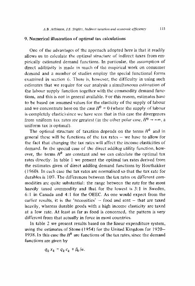
9. Numerical illustration of optimal tax calculations

One of the advantages of the approach adopted here is that it readily

allows us to calculate the optimal structure of indirect taxes from em-

pirically estimated demand functions. In particular, the assumption of

direct additivity is made in much of the empirical work on consumer

demand and a number of studies employ the special functional forms

examined in section 6. There is, however, the difficulty in using such

estimates that we require for our analysis a simultaneous estimation of

the labour supply function together with the commodity demand func-

tions, and this is not in general available. For this reason, estimates have

to be based on assumed values for the elasticity of the supply of labour

and we concentrate here on the case @ = 0 (where the supply of labour

is completely elastic) since we have seen that in this case the divergences

from uniform tax rates are greatest (in the other polar case, Ho + -00, a

uniform tax is optimal).

The optimal structure of taxation depends on the terms Hk and in

general these will be functions of the tax rates - we have to allow for

the fact that changing the tax rates will affect the income elasticities of

demand. In the special case of the direct addilog utility function, how-

ever, the terms Hk are constant and we can calculate the optimal tzx

rates directly. In table 1 we present the optimal tax rates derived from

the estimates given of direct addilog demand functions by Houthakker

(1960). In each case the tax rates are normalised so that the tax rate for

durables is 10%. The differences between the tax rates on different com-

modities are quite substantial: the range between the rate for the most

heavily taxed commodity and that for the lowest is 3: 1 in Sweden,

6: 1 in Canada and 4: 1 for the OEEC. As one would expect from the

earlier results, it is the ‘necessities’ - food and rent - that are taxed

heavily, whereas durable goods with a high income elasticity are taxed

at a low rate. At least as far as food is concerned, the pattern is very

different from that actually in force in most countries.

In table 2 we present results based on the linear expenditure system,

using the estimates of Stone (1954) for the United Kingdom for 1920-

1938. In this case the Hk are functions of the tax rates, since the demand

functions are given by

qkxk = qkck + @c/“.

116 A.B. Atkinson. J.E. Stiglitz, Indirect taxation and economic efficiency

Table 1

Optimal tax structure: direct addilog function.

Ad valorem tax rates (%) Sweden Canada O.E.E.C.

Food 29.6 21.4 26.9

Clothing 25.6 5.5 18.8 Rent 27.8 30.9 40.0 Durables 10.0 10.0 10.0 Other goods 29.6 31.3 24.4

Source: Calculations based on weighted mean estimates given in Houthakker (1960), table 2.

However, in the case where @ = 0, a is independent of the tax rate

and equation (3.5) reduces to the quadratic

This determines the optimal ad valorem tax rates fz (= 1 - (Pk/qk)),

and sample calculations are given in table 2 for a range of values of

Table 2

Optimal tax structure: linear expenditure system.

h/a = Ad valorem tax rates (%)

1.025 1.05 1.075

Commodity groups (1) Meat, fish, dairy products and fats 11.1 27.8 63.2 (2) Fruits and vegetables 8.2 18.6 33.4 (3) Drink and tobacco 10.1 24.1 48.5 (4) Household running expenses 5.3 11.4 18.2 (5) Durable goods 5.6 11.8 19.0 (6) Other goods and services 6.2 13.4 22.0

Notes: (a) Based on estimates given by Stone (1954), table 1 of ck, pk and l/o (= total expenditure

minus ‘committed’ expenditure).

(b) Relationship between producer and consumer prices based on that for 1938 as obtained

from National Income and Expenditure (1947). Groups (1) and (2) were combined for this purpose.

(c) Group (4) includes rent, fuel and light, non-durable household goods and domestic service.

Group (5) includes clothing, household durables, vehicles, transport .and communication

services,


X/a (reflecting different levels of revenue). (The sources of the estimates

of ck, ok, pk and 1 /a are described in the notes to table 2.) Again the

range of tax rates is wide and food (although not in this case housing) is

taxed much more heavily than durables.

It should be emphasised that these calculations are presented only to

illustrate the application of the theoretical approach developed in the

earlier sections. The use of alternative specifications of the demand

equations, or of alternative estimates of the same forms, may well give

rather different results.

10. Concluding comments

The principal conclusion we have reached is that if direct additivity

is a reasonable assumption for broad commodity groups, then the op-

timal structure of taxation from an efficiency viewpoint is one that

taxes more heavily goods which have a low income elasticity of demand.

This result generalises the conventional wisdom based on partial equi-

librium analysis, which can be obtained as a special case where the

supply of labour becomes completely elastic. Moreover, in terms of the

debate about the introduction of a uniform system of indirect taxes

referred to at the beginning of the paper, we have seen that there is no

general presumption in favour of uniform taxation on grounds of allo-

cative efficiency.

The analysis suggests two important areas for further research, which

we plan to examine in a sequel to the paper. Firstly, although we have

shown that uniform taxation cannot be justified by appeal to conside-

rations of allocative efficiency, it may still be true that the welfare loss

involved in using uniform rather than optimal taxes may be small. Se-

condly, the conclusion that goods with a low income elasticity should

be taxed heavily brings out very sharply the conflict between equity and

efficiency considerations. The recognition of equity objectives would

be expected to lead to important modifications of the conclusions. I7

” One important contribution of Diamond and Mirrlees (1971) is to extend the Ramsey- Samuelson analysis to the many-consumer case: however, like the analysis for the single consu-

mer, it does not readily allow conclusions to be drawn about which goods should be taxed more heavily.


Appendix

Equation (3.5) can be written

t$=ciqkCIHk +C,Uk,

x-a 1 where C, = ___

-Ho h-a 1

aX ___ C,= __-_ __ _ 1 --Ho’ 1-P x (y

SO

p-c k

C.U. x.-l-c 1 I lk I u 2 k

and

0 = - Cl pi UiXl .

These equations can be written

(t*, 0) = V(- qx, C,)’ )

where ’ denotes the transposition and

Hence (-4, X, C,) = V-‘(t*, 0).

But

where Sii denote the Slutsky terms. We thus obtain by inverting (3.5)

the familiar result

cisik ti = - Cl IC, Xk

obtained by Samuelson (195 1): the compensated demand for each good

should be reduced by the same proportion (for infinitesimal taxes).


References

Bishop, R.L., 1968, The effects of specific and ad valorem taxes, Quarterly Journal of Econo- mics 82, 198-218.

Boiteux, M., 195 1, Le ‘revenue distribuable’ et les pertes economiques, Econometrica 19, 112 - 33.

Cass, D. and J.E. Stiglitz, 1971, The structure of preferences and wealth effects in portfolio allocation, mimeo.

Corlett, W.J. and D.C. Hague, 1953, Complementarity and the excess burden of taxation, Review of Economic Studies 21, 21-30.

Diamond, P.A. and J.A. Mirrlees, 1971, Optimal taxation and public production, American Eco- nomic Review 61,8-27 and 261-278.

Dixit, A.K., 1970, On the optimum structure of commodity taxes, American Economic Review 60, 295-301.

Green, H.A.J., 1961, Direct additivity and consumers’ behaviour, Oxford Economic Papers 13, 132-136.

Harberger, A.C., 1964, Taxation, resource allocation, and welfare, in: The role of direct and indirect taxes in the federal revenue system (Princeton University Press).

Hicks, U.K. 1968, Public finance, 3rd ed. (London and New York, Cambridge University Press) . Houthakker, H.S., 1960, Additive preferences, Econometrica 28, 244-257.

Lerner, A.P., 1970, On optimal taxes with an untaxable sector, American Economic Review 60, 284-294.

Musgrave, R.A., 1959, The theory of public finance (New York, McGraw-Hill).

1947, National income and expenditure of the United Kingdom 1938 to 1946, H.M.S.O. Cmnd. 7099.

Prest, A.R., 1967, Public finance in theory and practice, 3rd ed. (Weidenfeld and Nicolson).

Ramsey, F.P., 1927, A contribution to the theory of taxation, Economic Journal 37, 47-61.

Samuelson, P.A., 1951, Memorandum for U.S. Treasury, unpublished.

Stiglitz, J.E. and P.S. Dasgupta, 1971. Differential taxation, public goods, and economic efficiency, Review of Economic Studies 38, 151-174.

Stiglitz, J.E., 1970, Taxation, risk taking, and the allocation of investment in a competitive economy, in: Jensen, M. (ed.), Studies in the theory of capital markets (forthcoming)

Stone, R., 1954, Linear expenditure systems and demand analysis: an application to the pattern of British demand, Economic Journal 64, 5 11-27.

Date post:	24-Jul-2018
Category:	Documents
Upload:	doandieu
View:	214 times
Download:	0 times

THE STRUCTURE OF INDIRECT TAXATION AND ECONOMIC...

Documents