The Structure of International Futures (IFs)

The Structure of International Futures (IFs)

Barry B. Hughes

with Anwar Hossain

Mohammod Irfan

Version 1.0. Feedback on this living document will be much appreciated.

Graduate School of International Studies University of Denver

May, 2004

Structure of IFs V1_0.doc

The Structure of International Futures (IFs )

Table of Contents

1. What Motivates International Futures (IFs)?.............................................................. 1 2. Basic Design Considerations ...................................................................................... 5

2.1 General Design Characteristics or Parameters.................................................... 5 2.2 Components of the Global System ..................................................................... 8 2.3 Philosophical Approach to Model Development.............................................. 10 2.4 Implementation Issues ...................................................................................... 13

3. Demographics ........................................................................................................... 15 3.1 Accounting System Elements: Stocks and Flows............................................ 16 3.2 Dominant Relationships.................................................................................... 18 3.3 Dynamics and Goal-Seeking............................................................................. 21

4. Economics................................................................................................................. 23 4.1 Production of Goods and Services.................................................................... 24 4.2 The Goods and Services Market ....................................................................... 28 4.3 The Social Accounting Matrix.......................................................................... 31

5. Energy....................................................................................................................... 41 5.1 Energy Resources.............................................................................................. 41 5.2 Energy Production ............................................................................................ 44 5.3 Energy Markets................................................................................................. 46

6. Agriculture ................................................................................................................ 57 6.1 Land Use ........................................................................................................... 57 6.2 Agricultural Production .................................................................................... 61 6.3 The Food and Agricultural Markets.................................................................. 64

7. The Environment ...................................................................................................... 67 7.1 Carbon Dioxide in IFs....................................................................................... 67 7.2 Water in IFs....................................................................................................... 69

8. Socio-Political Systems ................................................................................................ 72 8.1 Values and Culture............................................................................................ 74 8.2 Life Conditions ................................................................................................. 78 8.3 Socio-Political Processes and Institutions: Democratization............................ 81 8.4 Socio-Political Processes and Institutions: State Failure ................................. 85 8.5 Global Politics................................................................................................... 89

9. Conclusions................................................................................................................... 94 Bibliography ..................................................................................................................... 95

Structure of IFs V1_0.doc ii

Abstract

This paper provides a basic survey of the structure of the International Futures (IFs) modeling system. It touches briefly on motivation, purposes, and design considerations that have given rise to the IFs system and directed its evolution. It then provides a basic introduction to each of the component submodels of IFs, directing interested readers to more information as desired.

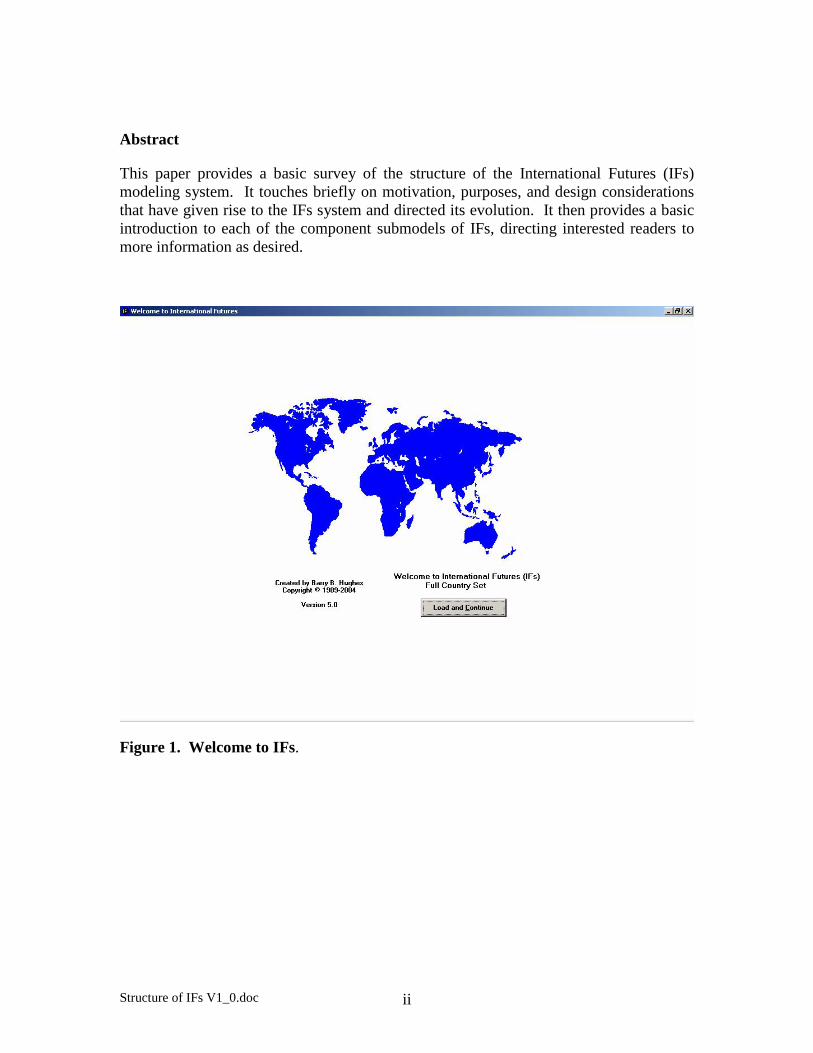
Figure 1. Welcome to IFs.

Structure of IFs V1_0.doc 1

1. What Motivates International Futures (IFs)?

International Futures (IFs) is a large-scale integrated global modeling system.1 The broad purpose of the International Futures (IFs) modeling system is to serve as a thinking tool for the analysis of near through long-term country-specific, regional, and global futures across multiple, interacting issue areas.

More specifically, IFs is a thinking tool, allowing variable time horizons up to 100 years, for exploring human leverage with respect to pursuit of key goals in the face of great uncertainty. The goals around which IFs was designed fall generally into three categories, as indicated by the figure below.

Human Development Humans as Individuals

Social Capacity for Fairness/Peace Humans with Each Other

Sustainable Material Well-Being Humans with the Environment

Figure 1.1 Goal Categories Motivating the Design and Use of IFs

The uncertainties of our future fall more or less into two primary categories. First, there are a substantial number of global transitions or transformations that we see on the horizon and that we pretty definitively know are coming. The uncertainties concern their timing and the dynamics of their unfolding. Global transformations and human leverage with respect to their management are special focal points for design of IFs, because such transformations almost invariably present special opportunities and challenges relative to more linear development patterns. The nearly certain transformations include:

Population aging, which offers opportunities for demographic dividends in the development process and for reduction of youth bulges, while posing great challenges for pension systems.

1 Current funding for IFs is coming from the National Intelligence Center and from Frederick S. Pardee. Recent developments to International Futures have been funded in substantial part by the TERRA project of the European Commission, by the Strategic Assessments Group of the U.S. Central Intelligence Agency, and by the RAND Frederick S. Pardee Center for Longer Range Global Policy and the Future of the Human Condition. In addition, the European Union Center at the University of Michigan has provided support for enhancing the user interface and ease of use of the IFs system. None of these institutions bears any responsibility for the analysis presented here, but their support has been greatly appreciated. Thanks also to the National Science Foundation, the Cleveland Foundation, the Exxon Education Foundation, the Kettering Family Foundation, the Pacific Cultural Foundation, the United States Institute of Peace, and General Motors for funding that contributed to earlier generations of IFs. Also of great importance, IFs owes much to the large number of students, instructors, and analysts who have used the system over many years and provided much appreciated advice for enhancement (some are identified in the Help system). The project also owes great appreciation to Anwar Hossain, Mohammod Irfan, and José Solórzano for data, modeling, and programming support within the most recent model generation, as well as to earlier student participants in the project (see again the Help system).


Movement of most of the world’s population from poverty to middle class and even higher income levels, which offers opportunities to meet targets such as the Millennium Development Goals with respect to human capabilities and well-being, but which will present large numbers of challenges including addressing the African development crisis/poverty trap.

Transition from fossil fuels to other energy forms, with substantial environmental benefits accompanying the transition but major challenges in structuring new energy systems to satisfying growing energy demands and to avoid substantial supply shocks and crises.

Democratization and broader socio-political development of most of the world’s peoples, which offers humans much more control of their destinies, but which will give rise during the transition to substantial social instability and value clash.

Adoption of environmentally sustainable life-styles and economic practices, which offers the possibility of reversing deforestation and addressing other environmental deterioration, but which also runs substantial risk of failing to come soon enough to avoid a number of environmental catastrophes including large-scale species loss, water crises, and global warming.

Power shift from Northern to Southern countries, which holds out the probability of redressing global imbalances that began arising early in the colonial and industrial eras, but which also means that the US and other currently more developed countries will experience power transitions to China, India, and other developing countries.

These and other major transformations of our world are highly probable in the current century and several are clearly underway. Doing nothing pro-actively will not stop most of them, and caution in action may in some cases be the best approach, but inattention puts at risk our ability to anticipate what have been called “inevitable surprises” with respect to the transitions and would forgo many opportunities to manage the transformations as successfully as possible.2 In a world where the magnitude of environmental impact by humans and the destructive power of their weapons systems have both risen dramatically, conscious attention to managing transformations appears especially desirable. The possibility of overshoot and collapse dynamics, especially around energy and environmental systems, makes a strong case for pro-active approaches on many issues.

The second class of uncertainties are the true wild cards: events or developments, some of which we might be able to name and place on a large list, but about which we have considerably less insight. They include breakthrough technologies, environmental tipping points, wars, and plagues. 2 Peter Schwarz (2003) has written of inevitable surprises. More generally, Pierre Wack (1985a, 1985b) and the Shell Scenario Group have emphasized the importance of understanding change, rebuilding mental models, and focusing attention on managing uncertainty while pursuing opportunity.


IFs assists with:

Understanding the state of the world and the manner in which the future appears to be unfolding

o Identifying tensions and inconsistencies that suggest political, economic and environmental risk in the near and middle term (a “watch list” functionality)

o Exploring longer-term trends and considering where they might be taking us

o Learning about the dynamics of global systems

Thinking about the future we want to see

o Clarifying goals/priorities

o Developing alternative scenarios (if-then statements) about the future, both with respect to the major transitions and possible wild card events

o Investigating the leverage various agent-classes may have in shaping the future and developing robust strategies for pursuing our preferred futures

A number of assumptions underlie the development of IFs. First, issues touching human development systems are growing in scope and scale as human interaction and human impact on the broader environment grow. This does not mean the issues are necessarily becoming more fundamentally insurmountable than in past eras. But it does mean that attention to the issues must have a global perspective, as well as local and regional ones.

Second, goals and priorities for human systems are becoming clearer and are more frequently and consistently enunciated. For instance, the UN Millennium Summit and the 2002 conference in Johannesburg (UNDP 2001: 21-24; UNDP 2002: 13-33) set specific goals for 2015 that include many focusing on the human condition. Such goals are increasingly guiding a sense of collective human opportunity and responsibility. Also, our ability to measure the human condition relative to these and other goals has improved enormously in recent years with advances in data and measurement.

Third, understanding of the dynamics of human systems is growing rapidly. As discussed later, IFs development has roots that go back to the 1970s. Understandings of the systems included in the IFs model are remarkably more sophisticated now than they were then.

Fourth, and derivatively, the domain of human choice and action is broadening. The reason for the creation of IFs is to help in thinking about such intervention and its consequences.

IFs is heavily data-based and also deeply rooted in theory. It represents major agent-classes (households, governments, firms) interacting in a variety of global structures (demographic, economic, social, and environmental). The system draws upon standard approaches to modeling specific issue areas whenever possible, extending those as necessary and integrating them across issue areas.


The menu-driven interface of the International Futures software system allows display of results from the base case and from alternative scenarios over time horizons from 2000 up to 2100. It provides tables, standard graphical formats, and a basic Geographic Information System (GIS) or mapping capability. It also provides specialized display formats for age-cohort demographic structures and social accounting matrices.

The system facilitates scenario development via a scenario-tree that simplifies changes in framing assumptions, wild-card event introductions, and agent-class interventions. Scenarios can be saved for development and refinement over time. Standard framing scenarios, such as those from the third study of the Intergovernmental Panel on Climate Change (IPCC), are available.

The modeling system also provides access to an extensive database for longitudinal and cross-sectional analysis. Insofar as possible, data represent 164 countries since 1960. In addition to providing a basis for developing formulations within the model, the database facilitates comparison of data with “historic forecasts” over the 1960-2000 period.

The remainder of this document provides additional information on the modeling system. By far the most extensive documentation is, however, available in the Help system of IFs itself. That includes full documentation through causal diagrams, equations, and computer code. See http://www.du.edu/~bhughes/ifs.html for access to the model.

http://www.du.edu/~bhughes/ifs.html


2. Basic Design Considerations

Given the goals of understanding human development systems and investigating the potential for human choice within them, how can we represent such systems in a formal, computer-based model such as International Futures (IFs)?

The answer to that question has at least four parts:

Identification of a basic set of design characteristics or parameters with respect to the model and the interface in which it is used.

Selection of the components of global systems that should be placed into submodels or modules of the total representation

Specification of a philosophical approach to representation of those global systems and their interaction that is theoretically-sound and also useful for analysis purposes

Determination of the technical approach to model development

The remainder of this chapter will consider each aspect of model development in turn.

2.1 General Design Characteristics or Parameters

The first set of four design parameter decisions concerns the model (M1-M4). The second concerns the interface (I1-I4).

M1. Geographic Representation. The most recent versions of IFs represent 164 countries individually, allowing the user to aggregate countries into flexibly-defined groupings of countries for display and analysis.

Most global models have represented at most 10-20 subregions of the world, some of which might be larger countries (like China or the United States). Initially, IFs took the same route, and the student edition of IFs continues to represent only 14 separate regions so as to minimize complexity of interaction and maximize model run speed.

Over time, however, the project has assembled a large associated database in support of IFs. That database now represents 164 countries for as many of the years as possible since 1960; the project has plans to move to 182 countries. It became obvious in the early 1990s that it was no longer productive to update periodically the initial conditions of the model through traditional manual processes, even with spreadsheets. Each time the base year of a large model is updated, such processes can absorb huge amounts of time. Early in that decade the IFs project developed what it calls a “pre-processor,” that takes data from the raw database and uses algorithms and functions to prepare a new set of initial conditions for the model. Thus when the data became available for 2000 and were in the database, the preprocessor was used to move the base year of the model forward without a great deal of effort.


A side benefit of the preprocessor is that the aggregation rules built into it for creating regions of the model could accommodate different regionalizations quite easily. Initially, IFs offered flexible aggregation in up to 20 different regions defined by the user. Then the project moved the limit up to 60 regions, and most recently it has removed the limit. At the same time, however, as the number of regions and countries expanded, it became increasingly important to allow the user to group regions and/or countries for display and analysis. The grouping system is now fully flexible as well.

M2. Issue-Area Representation. IFs represents demographic, economic, energy, food, environmental, and socio-political systems and subsystems, with extensive linkages among them and technological change occurring across all systems. The next section of this chapter will provide an overview of those systems.

IFs began with demographic, economic, energy and food systems, following in the footsteps of earlier world modeling. Over time, somewhat more substantial representation of environmental systems has come into being and technological change has been introduced as a distributed element across other subsystems.

Most importantly and distinctively relative to other world models, domestic and international socio-political representations have grown over time and have become quite substantial components of the IFs modeling system.

M3. Time Horizon. IFs allows model runs and analysis through 2100, but also allows users to shorten the horizon as desired.

It is difficult to look at important global transitions, such as those unfolding in demography, in energy and, hopefully, in the human relationship to the environment, without looking out to the end of the twenty-first century. At the same time, there are increasingly large numbers of users of the system for whom long-term analysis is a more traditional 10-20 years.

M4. Data and Theory Foundations. IFs uses an extensive database with several hundred series. It also draws heavily theory across the issue areas it represents.

Although short-term forecasts can rely heavily on extrapolation, that is obviously not possible in mid- and longer-term forecasting. The old saying that “a trend is a trend is a trend until it bends” is of special significance for longer-term forecasting, which must represent non-linear and non-extrapolative behavior. The third section of this chapter will return to the philosophy of the IFs project with respect to structural representations.

I1. Availability. Turning from the model proper to the interface and use of the model, the IFs project has long made the model readily available to multiple users.

The importance of accessibility of a model to users should not be underestimated. Most world models have either been unavailable outside of the projects that developed them or have become available only after the projects ended. The first versions of IFs were made available to students and professors in about 1980 on mainframe computers, and the first versions of IFs on microcomputers, with a menu interface, became widely available in


early 1990. Over the intervening period, the feedback provided by users has strongly shaped the development of the model. Although it would be ideal in the future of the project to involve users directly in ongoing model development, responsiveness to their suggestions for improvement of model and interface provides a tremendous base of ideas and incentives for improvements.

I2. User Friendliness. Availability is necessary, but insufficient. The IFs project has continued to make intervention in model assumptions easier, relying on a menu-driven graphical user interface in recent years.

The first generation of IFs, like most previous world models, was command driven. Users faced a cursor on a nearly blank screen and needed to understand the basic commands and the names of variables in order to do anything. When IFs moved to microcomputers it developed a menu-based system of the type familiar to MS Windows users. Although this system still requires too many clicks to achieve many of its functions, it has continued to evolve and to become simpler to use, even as functionality became richer. For instance, there is an extensive, context-sensitive Help system. There is no other world model with the availability and ease of use that IFs offers.

I3. Interventions and Scenario Development. User friendliness is also insufficient. IFs offers users a variety of tools for changing assumptions of the model and developing new scenarios. Among these tools is a growing library of pre-packaged scenarios.

Even quite early versions of IFs provided the ability to change any parameter or initial condition and to do so with time-varying specificity, if desired. The most recent versions have developed two important additional features. One is the scenario tree, allowing the user to explore for relevant interventions without knowing or searching for variable names. The second is the capability of saving and retrieving simple or complex scenarios, either those developed by others or those developed or modified by individual users.

I4. Transparency and Openness. Although the IFs project has not yet done enough in this arena, the in-system documentation of structures and formulations is extensive and readily available. Increasingly also, the user can change formulations, making the model somewhat more open.

Standard advice in forecasting is to use simple rather than complex models, in part because the user is often hard-pressed to understand the behavior of more complex ones, giving them a black-box character. That is good advice, except that long-term, multi-issue global models cannot possibly follow it. The alternative is to strive for transparency and openness in other ways. With respect to transparency, IFs does so by putting detailed causal diagrams, equations, and even the computer code itself into the Help system. Increasingly, the project has developed techniques to make the portions of these specific to particular parameters and variables available to users on demand. With respect to openness, IFs has always made it possible to change parameters on demand. More recently, it has made many of its bi-variate formulations available for change as desired by the user. Most recently it has begun to extend that capability to multi-variate


formulations. Ideally, users should be able to append their own modules to IFs or even to replace modules of IFs with their own structures. Such a vision is some considerable distance from current reality.

The last chapter of this report will return to some of these basic design parameters/characteristics in the form of a discussion of visions for the future of world modeling.

2.2 Components of the Global System

This section turns to the coverage of issue areas within the global system and to the general shape of modules within IFs. Figure 2.1 shows the major conceptual blocks of the International Futures system. The elements of the technology block are, in fact, scattered throughout the model. The arrows and named linkages between blocks are illustrative, by no means exhaustive.

Economic

Socio-Political

Population

Agriculture Energy

EnvironmentalResources and

Quality

International Politcal

Labor

Demand, Supply,Prices, Investment

Resource Use,Carbon Production

Land Use,Water

GovernmentExpenditures

Conflict/CooperationStability/Instability

FoodDemand

Income Networking

Technology

May 2002

Figure 2.1 An Overview of International Futures (IFs)

The population module:

represents 22 age-sex cohorts to age 100+ in a standard cohort-component system structure

calculates change in cohort-specific fertility of households in response to income, and income distribution


calculates change in mortality rates in response to income, income distribution, and assumptions about technological change affecting mortality

computes average life expectancy at birth, literacy rate, and overall measures of human development (HDI) and physical quality of life

represents migration shows HIV/AIDS includes a newly developing submodel of formal education across primary,

secondary, and tertiary levels

The economic module:

represents the economy in six sectors: agriculture, materials, energy, industry, services, and ICT (other sectors could be configured, using raw data from the GTAP project)

computes and uses input-output matrices that change dynamically with development level

is a general equilibrium-seeking model that does not assume exact equilibrium will exist in any given year; rather it uses inventories as buffer stocks and to provide price signals so that the model chases equilibrium over time

contains a Cobb-Douglas production function that (following insights of Solow and Romer) endogenously represents contributions to growth in multifactor productivity from R&D, education, worker health, economic policies (“freedom”), and energy prices (the “quality” of capital)

uses a Linear Expenditure System to represent changing consumption patterns utilizes a "pooled" rather than the bilateral trade approach for international trade has been imbedded in a social accounting matrix (SAM) envelope that ties

economic production and consumption to intra-actor financial flows

The agricultural module:

represents production, consumption and trade of crops and meat; it also carries ocean fish catch and aquaculture in less detail

maintains land use in crop, grazing, forest, urban, and "other" categories represents demand for food, for livestock feed, and for industrial use of

agricultural products is a partial equilibrium model in which food stocks buffer imbalances between

production and consumption and determine price changes overrides the agricultural sector in the economic module unless the user chooses

otherwise

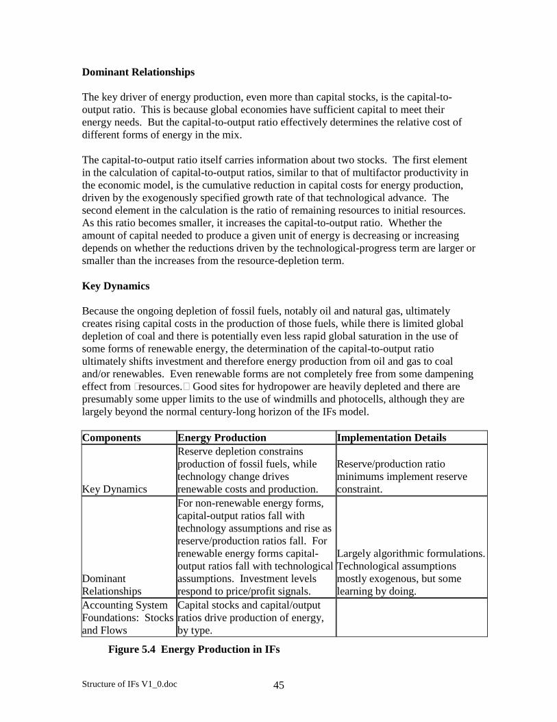
The energy module:

portrays production of six energy types: oil, gas, coal, nuclear, hydroelectric, and other renewable energy forms

represents consumption and trade of energy in the aggregate represents known reserves and ultimate resources of the fossil fuels portrays changing capital costs of each energy type with technological change as

well as with draw-downs of resources


is a partial equilibrium model in which energy stocks buffer imbalances between production and consumption and determine price changes

overrides the energy sector in the economic module unless the user chooses otherwise

The socio-political sub-module:

represents fiscal policy through taxing and spending decisions shows six categories of government spending: military, health, education, R&D,

foreign aid, and a residual category represents changes in social conditions of individuals (like fertility rates or

literacy levels), attitudes of individuals (such as the level of materialism/postmaterialism of a society from the World Values Survey), and the social organization of people (such as the status of women)

represents the evolution of democracy represents the prospects for state instability or failure

The international political sub-module:

traces changes in power balances across states and regions allows exploration of changes in the level of interstate threat

The environmental module:

allows tracking of remaining resources of fossil fuels, of the area of forested land, of water usage, and of atmospheric carbon dioxide emissions

provides a display interface for the user that builds upon the Advanced Sustainability Analysis system of the Finland Futures Research Centre (FFRC), Kaivo-oja, Luukhanen, and Malaska (2002)

The implicit technology module:

is distributed throughout the overall model allows changes in assumptions about rates of technological advance in

agriculture, energy, and the broader economy explicitly represents the extent of electronic networking of individuals in societies is tied to the governmental spending model with respect to R&D spending

2.3 Philosophical Approach to Model Development

The representation of global systems, such as those identified above, benefits from a philosophical understanding of the character of those systems and our ability to represent them. The approach of IFs builds on basic propositions:

Global human systems consist of classes of agents and larger structures within which those agents interact. Among key agent classes of interest, in part because they can be the target of policy interventions, are households, firms, and governments. They also increasingly include intergovernmental organizations (IGOs) and non-governmental organizations (NGOs).


Many, although not all, of the structures within which humans interact involve stocks and flows of elements such as people, goods and services, money, materials, and knowledge.

Many of the primary or dominant relationships in global systems determine flows, because those flows reshape structures over time. Clearly, some flows are more important than others and require particular attention.3

Human systems are dynamic, making it important to represent key dynamics of human systems that are equilibrating or that create disequilibrium.

No straitjacket should be imposed on the representation of human systems. For instance, many processes are very difficult to represent in terms of agent-classes and benefit from representation in terms of more aggregate processes of change.

Consider, for instance, the representation of demographic systems. It is possible simply to extrapolate population or to represent population as a growth process with a constant or variable growth rate. Many models take such approaches.

Demographers have, however, developed representations of human populations that illustrate the above propositions. They typically represent the structures through age-sex cohort distributions of population (stocks) with births, deaths, and migration (flows) changing those stocks over time. Households are key agents that make decisions to have children or to emigrate. Although fertility and mortality patterns can create rough equilibrium within societies, there are key dynamics around each that very often lead to disequilibrium.

Similarly, households, firms, and governments interact in larger economic and socio-economic systems or structures. A model can represent the behavior of households with respect to use of time for employment and leisure, the use of income for consumption and savings, and the specifics of consumption decisions across possible goods and services. It can represent the decisions of firms with respect to re-investment or distribution of earnings. Markets are key structures that integrate such activities, and IFs represents the equilibrating mechanisms of markets in goods and services.

In addition, however, there are many non-market socio-economic interactions. IFs increasingly represents the behavior of governments with respect to search for income and targeting of transfers and expenditures, domestically and across country borders, in interaction with other agents including households, firms, and international financial institutions (IFIs). Social Accounting Matrices (SAMs) are structural forms that integrate representation of non-market based financial transfers among such agents with

3 Mihajlo Mesarovic made clear the importance of emphasizing dominant relationships in the course of the TERRA project and during the development of IFs for TERRA. At the same time, however, attention to dominant relations without rooting that attention in a representation of stocks and flows and without attention to system dynamics can lead to focus on unconstrained behaviour and to conclusions about disequilibrium/imbalances that would not be warranted in the context of a more complete analysis.


exchanges in a market system. IFs uses a SAM structure to account for inter-agent flows generally. Financial asset and debt stocks, and not just flows, are also important to maintain as part of this structural system, because they both make possible and motivate behavior of agent-classes.

Further, governments interact with each other in larger inter-state systems that frame the pursuit of security and cooperative interaction. Potential behavioral elements include spending on the military, joining of alliances, or even the development of new institutions. One typical approach to representing such structures is via action-reaction dynamics that are sensitive to power relationships across the actors within them. IFs represents changing power structures, domestic democracy level, and interstate threat.

Still further, human actor classes interact with each other and the broader environment. In so doing, important behavior includes technological innovation and use, as well as resource extraction and emissions release. The structures of IFs within which all of these occur include a mixture of fixed constraints (for instance, non-renewable resources), uncertain opportunities for technological change in economic processes, and systems of material flows.

Components Explanation Implications (Good; Bad)

Key Dynamics Equilibrium-seeking and disequilibrium-causing

Non-linear behavior producible; Analysis and tuning necessary

Dominant Relationships

Agent-class behavior by households, governments, firms when possible; aggregate when not

Leverage points accessible; Eclectic, evolving formulations necessary (estimations, stylized facts, algorithmic)

Accounting System Foundations: Stocks and Flows

Population; Land; Capital; Goods/Services; Assets/Liabilities; Materials; Knowledge

Intervention consequences meaningfully tracked;

Data/structure intensive

Figure 2.2 The Philosophical Foundations of International Futures (IFs)

Figure 2.2 summarizes the philosophic foundations and approach of IFs, as discussed above. It also draws some implications concerning the IFs approach. For instance, the representation of stocks and flows provides accounting structures that are very important in tracing immediate and longer-term consequences of interventions. Thus a government transfer payment from one type of household to another has consequences in terms of other flows and underlying stocks (such as government debt). At the same time, however, such stock and flow structures are very data and structure intensive.

Similarly, a positive implication of a focus on dominant relationships, particularly those that can be represented in terms of agent-class behavior, is that leverage points become


available for exploration of policy interventions. A negative implication is those dominant relations often require complex representation – it is often easier to think about humans following algorithms or rules than to think about them behaving according to estimated equations.4

With respect to key dynamics, the benefit of representing them is the ability to capture the non-linearities that obviously characterize long-term global systems. A related complication is that dynamic systems within models inevitably require that the modeler return again and again to analysis and adjustment of their behavior.

In summary, International Futures (IFs) has foundations that rest in (1) classes of agents and their behavior and (2) the structures and dynamic systems through which those classes of agents interact. IFs is not agent-based in the sense of models that represent individual micro-agents following rules and generating structures through their behavior. Instead, as indicated, IFs instead represents both existing macro-agent classes and existing structures (with complex historic path dependencies), attempting to represent some elements of how behavior of those agents can change and how the structures can evolve.5

2.4 Implementation Issues

Although it has become less common, the traditional question asked of a modeler often was “what kind of modeling do you do?” The correct answers were generally assumed to be econometrics, systems dynamics, or some form of optimization (linear programming). In recent years the set of correct answers has been expanded to include agent-based modeling or more macro/structural approaches. “Eclectic” has not generally been considered a correct answer. Yet the best description of the IFs approach is probably “structure-based, (increasingly) agent-class driven, dynamic modeling.” Although IFs is not an econometric model, it does rely heavily on data and uses estimation of relationships quite heavily. Although IFs is not a systems dynamics model, it pays careful attention to stocks, flows and the dynamics that their interactions set up. The reader of this document will find that IFs represents global processes in terms of both nested and overlapping systems. That is, in some cases systems (such as the representation of fossil fuel resource discovery and use) are fully nested in larger systems (such as the broader energy model). In other cases systems are

4 Agent-based modelling is correct in emphasizing such rules. Agent-class behaviour cannot rely solely on rules, but can be attentive to them as well as to the representation of macro patterns of behaviour. As modelling moves towards more algorithmic representation of agent-class behaviour, structural modelling may also begin to see emergent properties from that behaviour.

5 Philosophically, this approach rejects the premise that all model structures must be built up from micro-agent interaction. Although micro-agent modeling is laudable in more narrowly-focused models, global systems and structures are far too numerous and well-developed for such efforts to succeed across the breadth of concerns in IFs, at least given contemporary modeling capabilities.


overlapping or intersecting, such as the economic and socio-political systems.6 And although IFs is far from an optimization structure, it pays much attention to the appropriate desire of those studying complex systems to explore for strategies that improve futures. Finally, while IFs increasingly attempts to build relationships around agent-classes and rules of agent behavior, it is definitely not micro-agent based. Other common questions asked of modelers is “do you use differential or difference equations?” and “what kind of closure do you use?” IFs uses difference equations, with a recursive structure and 1-year time steps. Although differential equations with simultaneous solution (using explicit closure rules) may be more mathematically sophisticated than recursive difference equations, it is not clear that simultaneous differential approaches actually introduce more accuracy or real-world verisimilitude. For example, it is not clear that the precise equilibria to which they can give rise exist in the real world; the premise of IFs is that in most systems, agents are “chasing equilibrium” over time, a process that suggests that modeling the pursuit of equilibrium within recursive systems may be more nearly comparable to reality. Solution techniques for differential equations in large-scale models nearly always involve computational intensity that greatly slow down the exploration of model behavior under alternative interventions. That leads to a third question that ought to be asked of modelers even more often than it is: “how easy is it to intervene in your model and explore the implications of such intervention?” In the case of IFs, the extensive interface makes that much easier than in most models. And the widespread availability of the system is an additional advantage of real importance.

This chapter has addressed basic design considerations at a general level. The next chapters turn to the structure of the model and will thereby elaborate the introduction provided here.

6 Advice was once common to make all systems in some way hierarchical, if not in authority, at least in logic. IFs has chosen not to follow that advice, because systems are simply not always hierarchical.


3. Demographics

The demographic submodel of IFs uses the standard cohort-component methodology of larger-scale demographic forecasting systems like those of the United Nations and the U.S. Census Bureau. Specifically, IFs represents the stocks of population in each geographic unit with a standard age-sex distribution, distinguishing females and males across 22 cohorts (infants, five-year intervals up to age 99, and those aged 100 or over). The model uses an age-specific distribution of fertility and an age-sex specific distribution of mortality to calculate annual births and deaths (population flows). It also calculates age-sex specific migration.

The dominant relationships of the demographic submodel are those that determine the flows, namely relationships that specify fertility, mortality (including swings in mortality related to the HIV/AIDS epidemic), and migration. The single most important relationship of the demographic model is almost certainly the representation of total fertility rate, which is imposed on the fertility distribution to calculate annual births. The calculations of life expectancy and of excess deaths from AIDS are also of considerable importance, but changes in longevity, except those that affect people before child-bearing years, typically have less impact on long-term demographic patterns than do changes in numbers of births.

Contemporary societies pay attention to demographic totals and distributions and there has been clear goal-seeking behavior in many countries with respect to fertility reduction. Although there is now considerable discussion with respect to the problems associated with below-replacement fertility, it is not clear that societies will be able to pursue any kind of population equilibrium in the longer term. Moreover, it is not clear what equilibrium levels would be pursued. Thus the model incorporates only very weakly goal-seeking long-term dynamics.

The figure below summarizes these basic characteristics of the demographic submodel. The rest of this chapter elaborates key elements of it and the Help system of IFs provides full detail.


Components Demographics Implementation Details

Key Dynamics and Goal-Seeking

No equilibration stabilizes population. Long-term fertility rates, life expectancy, and peaks of HIV/AIDS are uncertain.

Base patterns adjusted to UN forecasts; scenarios used for uncertain patterns.


Fertility rate primary. Life expectancy secondary. Migration tertiary. HIV/AIDS a wildcard.

Fertility and mortality (life expectancy) are cross-sectionally estimated functions with additional time-shift terms. HIV/AIDS is algorithmic, using approach of UNAIDS.


Cohort-component age-sex structure with births, deaths, migration.

22 age-sex cohorts to age 100+. Separate age-sex, fertility and mortality distributions.

Figure 3.1 The Basic Structures of Demographics in IFs

3.1 Accounting System Elements: Stocks and Flows

The stocks of International Futures are people, by age and sex. Figures 3.2 and 3.3 show examples of the standard age-sex distributions that track these, aggregated for non-OECD and OECD countries. IFs produces such distributions by country and aggregated region or country grouping and across time, for the base case and for any desired scenario. It also produces distributions of fertility and mortality. The processes of determining births and deaths and of advancing the population distribution across time are essential core structures for the IFs demographic representation.


Population Distribution for non-OECD in Year 2000[Base Case]

Males

Females

Population in Millions

0- 4

5- 9

10- 14

15- 19

20- 24

25- 29

30- 34

35- 39

40- 44

45- 49

50- 54

55- 59

60- 64

65- 69

70- 74

75- 79

80- 84

85- 89

90- 94

95- 99

100+

Figure 3.2 An Age-Sex Distribution from IFs for non-OECD Countries

Population Distribution for OECD in Year 2000 [BaseCase]

Males

Females

Population in Millions

0- 4

5- 9

10- 14

15- 19

20- 24

25- 29

30- 34

35- 39

40- 44

45- 49

50- 54

55- 59

60- 64

65- 69

70- 74

75- 79

80- 84

85- 89

90- 94

95- 99

100+

Figure 3.3 An Age-Sex Distribution from IFs for non-OECD Countries


3.2 Dominant Relationships

As indicated above, the key relationship in the demographic model is probably that which determines the total fertility rate. Among the variables that are most often suggested to be important in that determination are the GDP per capita, levels of education (especially for females) and contraception use or family planning program strength more generally.

Using data from the IFs database, the cross-sectional relationship between such factors and fertility can be examined. Table 3.1 shows several alternative estimations of that relationship based on data as near as possible to the year 2000 (although some analysts would call those estimations “models,” we reserve that word here for dynamic systems. Estimations 1a through 1c all begin with logged GDP per capita at purchasing power parity (PPP). That variable by itself explains 56% of the variation in the total fertility rate (TFR) across countries in 2000. When the average years of total education for people 25-years old or older are added, the variation explained exceeds 76%, and the rate of contraception use increases it still further (but with a reduction in T-scores and significance probabilities below desired levels).

Estimations 2a through 2c begin with years of education. Estimations 2a and 2b contrast the explanatory power of female education alone with that of education for the entire population, and it is the latter which gives the higher adjusted r-squared. Adding contraception use to education years produces an explained variation of 82%, a remarkably high number.

Which estimation should IFs use? The easy answer would be estimation 2c. Not only does it produce the highest level of variance explained, but it also relies on two variables that both offer immediate leverage for policy interventions intended to influence fertility.

Estimation Adjusted

R-squared GDP per

capita (PPP) Education

Years Total Education

Years Female Contraception

Use 1a 0.560 -13.96 (log)

1b 0.763 -6.97 (log) -2.27

(p<.024)

1c 0.789 -1.42 (log) -1.41

(p<.165) -5.76

2a 0.649 -11.91 2b 0.713 -16.25 (log) 2c 0.824 -4.94 (log) -7.27

Table 3.1 Estimations for Explaining Total Fertility Rates (values in variable cells are T-scores)

But modeling is an art, not a science and the easy answer is not always the best. The education model within IFs is still under development (by Mohammod T. Irfan) and is not yet as solid in its own forecasts as desired. Thus selecting an estimation like 2b or 2c, based heavily on it, has some real disadvantages that may disappear as the model is further developed. At the time of this writing, the estimation used was 1b, giving dominant driving power to GDP per capita and secondary influence to education. The


IFs system represents this particular relationship, however, and an increasing numbers of others as a multivariate function accessible to the user, so that the variables included and the character of the formulation can be changed.

Another complicated issue in modeling that requires judgment rather than strict attention to r-squared and significance levels is the handling of important driver variables that do not make statistical cuts. Clearly, for example, in spite of the significance levels for model 1b, both estimations 1c and 2c suggest that contraception use may be important in forecasting fertility. One approach to handling such drivers is not to include them in the basic formulation, but to add them to an extended formulation in a more algorithmic or rule-based fashion (trying to use good judgment and common sense). Thus in the implementation of the basic estimation 1b in IFs, the relationship has been extended by a formulation that incorporates the apparent rate of reduction of fertility for each percentage point rise in contraception use, controlling for level of GDP per capita; since GDP per capita and contraception use are highly correlated, the implementation calculates expected contraception use at a given level of GDP per capita, and shifts fertility as use deviates from that expected level. The extension of the basic formulation can be turned off by a model user.

In addition, actual fertility data for countries often deviates from the rate that would be calculated from estimation 1b, with or without extension. It makes no sense to forecast a value of fertility for a country in the year 2000 that differs from actual data. Thus the implementation of the formulation computes a shift factor in the initial year that represents the deviation of the formula’s computation from data and applies that shift over time. As in this instance, IFs often allows the shift factor to decay over a long period of time, moving computed values towards those of the formulation.

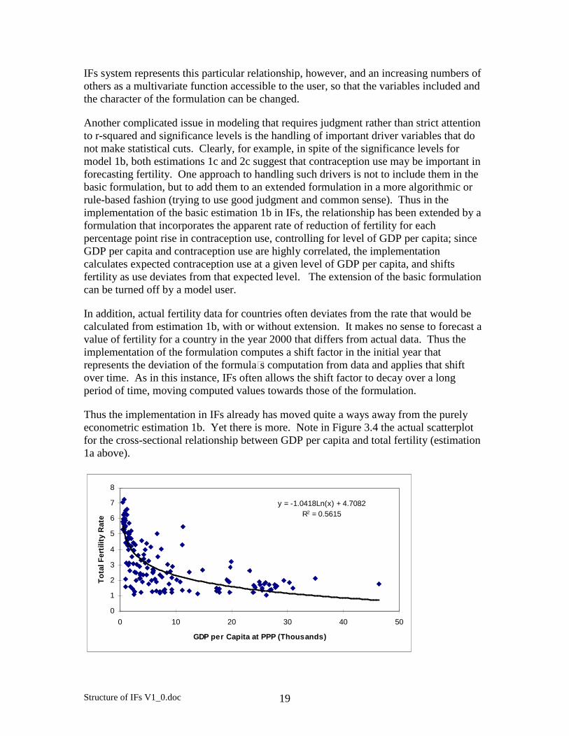
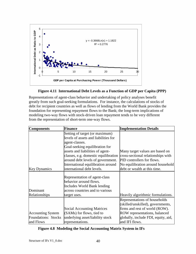
Thus the implementation in IFs already has moved quite a ways away from the purely econometric estimation 1b. Yet there is more. Note in Figure 3.4 the actual scatterplot for the cross-sectional relationship between GDP per capita and total fertility (estimation 1a above).

y = -1.0418Ln(x) + 4.7082R2 = 0.5615

0

1

2

3

4

5

6

7

8

0 10 20 30 40 50

GDP per Capita at PPP (Thousands)

To

tal F

erti

lity

Rat

e


Figure 3.4 Cross-Sectional Estimation of Fertility from GDP per Capita

Figure 3.5 shows that same relationship at three points in time: 1960, 1980, and 1998. It is obvious in Figure 3.5 that a downward shift in fertility at all levels of GDP per capita has occurred over time. Part of this could be a result of rising education levels and/or contraception use, factors picked up in estimations 1b and 1c. But it is likely that most of it is not a function of those other variables. For one thing, those variables themselves are highly correlated with GDP per capita – what is being picked up in estimations 1b and 1c is the impact of deviation in education and contraception around what would be expected at particular levels of GDP per capita.

GDP/Capita (PPP) VersusTotal Fertility Rate (1960)



0.00

1.22

2.44

3.66

4.88

6.10

0 10 20 30 40

Figure 3.5 Comparative Cross-Sectional Estimations of Fertility

What then has caused the downward shift of the function over time? Two reasonable hypotheses are improvements in contraceptive technology (making it easier to use, more effective, and cheaper) and the global regime around family planning, in which the idea has spread over time that family planning is acceptable practice, good for families and countries. Neither of these two hypotheses is easy to quantify or translate into estimated coefficients for forecasting.

Rather than leave the downward shift of the curve out of the formulation of the relationship, however, a time dependent-factor was added on top of the formulation described above. How big should that shift be in the future? Almost certainly it should be smaller than in the past and should decay over time because of obvious saturation effects. In practice the factor was determined in IFs partly by a process of what is called tuning, the adjustment of the factor so as to produce a base case forecast that is not far from the median-variant forecast of the UN in its most recent release.

The point of describing this complicated and somewhat messy process of implementing a key relationship in IFs is to show that the formulation of this and other dominant relationships in IFs is not, and cannot be a simple process of statistical estimation, and that it must most often combine estimation with insight and common sense in a formulation that takes on a kind of algorithmic (logical procedure) character. Insofar as possible, all such relationships ought also to be transparent to model users and changeable by them.


Life expectancy in IFs does not affect the long-term model dynamics as much as fertility, but is still an important function. IFs again computes a basic formulation from cross-sectional analysis against GDP per capita, and again the r-squared is high. In forecasting long-term life expectancy there clearly are two additional and interacting factors that need consideration. The first is advance in medical technology, which has steadily added years of average life expectancy in countries independently of GDP per capita. The second is the uncertainty of experts with respect to the genetic potential for continuing that addition of years. IFs once again has added a time dependent-factor on top of the basic estimation. It was tuned so as to provide expansions of life expectancy comparable to those forecast by the UN over the first half of the century. There are, however, futurists who anticipate much greater extensions of life expectancy with new insight into genetics. IFs relies upon scenarios to introduce such assumptions.

A fully separate representation of HIV/AIDS lets model users easily alter patterns of the epidemic’s unfolding. The basic representation identifies an estimate of the year for each country in which the epidemic will peak and the rate of infection that will characterize the peak year (using UN AIDS estimates for both, when available). Infection rates grow with a gradually saturating pattern from initial conditions to the peak year and then decay slowly from the peak.

Migration is a third flow of population into and out of country-specific stocks. The base formulation in IFs relies on UN estimates of rates of migration, which are in turn heavily built on data from recent years. Such rates cannot, however, be used without change across the century. Thus IFs arbitrarily introduces two basic constraints upon the rates over time. First, because large population movements have not been historically sustainable over long periods of time, the maximum inflow or outflow of population is reduced over about 20 years to one percent of a country’s population. Second, because it has almost always been rapidly growing populations that have provided the bulk of immigrants, the rate of outflow is reduced if it would result in an absolute population decline of more than 0.5%.

In the representation of inter-country flows of any kind, the sum across countries of calculations of flows out will seldom be exactly identical to the calculations of flows in. In most such cases IFs relies on a simple reconciliation process to maintain global balances. It calculations the sum of outflows and the sum of inflows, averages the two to determine the global flow to be used, and then normalizes country-specific values to that global value. This is the procedure used for migration. As is almost always the case, the interface allows the user to intervene to change patterns from those of the basic formulation.

3.3 Dynamics and Goal-Seeking

The latter part of the discussion above around the formulation for fertility began to move logically into a discussion of long-term dynamics of the demographic module. A key question in long-term population forecasting surrounds the rate of fertility in countries where it has dropped significantly below replacement fertility or may do so. Will it stay well below replacement level or will it rise again towards, to, or above it? Long-term UN


high, median, and low scenarios explicitly specify values that range from ¼ child above to ¼ child below replacement.

Such specification, which essentially builds in long-term behavior rather than computing it in some way, is the correct way to proceed. Long-term modelers must “own” long-term dynamics. That is, they must understand them, control them, and let users change them, not simply look at the result of complex formulations and report them to the world.

With respect to IFs and the time horizon of the 21st century, a conscious decision was made not to force long-term total fertility rates towards replacement fertility, but to let those rates fall towards and below replacement for currently developing countries and to begin bringing them back up towards but not to replacement as the century proceeds (the extent of approach towards replacement is controlled by an exogenously accessible parameter). One key aspect of this specification is that for most of the forecast horizon developing countries continue to exhibit fertility declines, while currently more developed countries begin to exhibit fertility increases, leading to some degree of convergence of the rates in the two country sets.


4. Economics The economic structure of IFs combines the features of dynamic computable general equilibrium models (CGEs) with the representations of social accounting matrices (SAMs). IFs models the economies for each of its geographic countries/regions in terms of six sectors (agriculture, energy, primary materials, manufactures, services, and ICT) and two household types (unskilled and skilled). The model uses Cobb-Douglas production functions with endogenous representation of change in multifactor productivity and linear expenditure system (LES) functions for change in household consumption patterns. Production, consumption, and exchange of goods and services come together in the representation of a market for goods and services that relies on changes in inventory stocks and price signals to pursue equilibrium over time. The SAM structure adds government revenue and spending decisions to the household and firm-based agent-class structure of the goods and services market. The SAM also maintains consistency in all inter-agent flows, including those with the rest of the world and across all countries/regions of the world. IFs uses a pooled rather than dyadic or bilateral representation of trade and other inter-country flows including foreign aid and foreign direct investment. Further, the SAM tracks assets and liabilities of governments and other agents as stocks, linking the levels of those stocks to behavioral representations of flows. IFs represents the agricultural and energy sectors of the model with physical or bottom-up, partial equilibrium modules, to be discussed in subsequent chapters. Monetary values calculated from the physical values of the partial equilibrium models enter into and override those of appropriate sector of the multi-sector economic model. As in other areas of IFs, the economic model can usefully be understood in terms of (1) accounting foundations that represent stocks and flows in a manner that facilitates tracking of the impact of interventions, including behavior of agent classes, (2) the formulations of dominant relationships that determine behavior, and (3) approach to key dynamics that characterize the integrated system. It is, however, difficult to conceptualize the full economic model at one time, even using this organizational hierarchy. It is useful to present the full economic model in three steps. The first step considers the production of goods and services. In many respects this remains the dynamic core of the economic model because it determines the growth rate and size of the economy in the long run. The second step broadens attention to the larger goods and services market, which incorporates consumption and exchange, as well as production. The third step expands attention further to the full social accounting system, with financial exchanges among agent classes and across geographic units. Obviously, the full economic model is tightly integrated across the three levels of presentation: for instance, spending by governments on education affects production of goods and services.


The rest of this chapter considers each of these elements in turn.

4.1 Production of Goods and Services

Accounting System Elements: Stocks and Flows IFs uses a Cobb-Douglas production function with disembodied technology/human capital maintained as multifactor productivity. Capital stocks are maintained by economic sector, but not by vintage, and capital stocks are not substitutable across sectors. Capital depreciates over time and the flow of new investment, driven by domestic savings and inflows from abroad augments it. Labor is driven primarily by the size and age structure of the population and by participation rate, with change in female participation rates treated explicitly. Like capital and labor, multifactor productivity has the character of a stock, augmented or decreased by an endogenously computed annual change. Dominant Relationships The character of the production function and the relationships around the growth or decline of capital and labor stocks are important relationships and the Help system of the model fully describes them. Because it has been shown repeatedly since Solow’s original residual analysis that technical progress normally accounts for 50 percent or more of growth, the key relationship in terms of the long-term dynamics of the model is the growth of multifactor productivity.

Solow (1956) recognized that the then-standard Cobb-Douglas production function with a constant scaling coefficient in front of the capital and labor terms was inadequate, because the expansion of capital stock and labor supply cannot account for most economic growth. It became standard practice to represent an exogenously specified growth of technology term in front of the capital and labor terms as "disembodied" technological progress (Allen, 1968: Chapter 13). Romer (1994) began to show the value of unpacking such a term and specifying its elements in the model, thereby endogenously representing this otherwise very large residual, which we can understand to represent the growth of productivity.

In IFs that total endogenous productivity growth factor (TEF) is the accumulation over time of annual values of growth in multifactor productivity (MFPGRO). There are many components contributing to growth of productivity, and there is a vast literature around them. See, for example, Barro and Sala-i-Martin (1999) for theoretical and empirical treatment of productivity drivers; also see Barro (1997) for empirical analysis or McMahon (1999) for a focus on education.

Recognizing the importance of endogenizing productivity, there was a fundamental choice to make in the development of IFs. One option was to keep the multi-factor productivity representation very simple, perhaps to restrict it to one or two key drivers, and to estimate the endogenization as carefully as possible. Suggestions included


focusing on the availability/price of energy and the growth in electronic networking and the knowledge society.

A second option was to develop a representation that included many more factors known or strongly suspected to influence productivity and to attempt a more stylistic and algorithmic representation of the function, using empirical research to aid the effort when possible. The advantages of the second approach include creating a model that is much more responsive to a wide range of policy levers over the long term. The disadvantages include some inevitable complications with respect to overlap and redundancy of factor representation, as well as some considerable complexity of presentation.

Because IFs is a policy-oriented thinking tool and because many forces clearly to affect productivity, the second approach was adopted, and the production function has become an element of the model that will be subject to regular revision and enhancement. Those who want more detail and equations should turn to the Help system of the model or to Hughes and Anwar (September 2003). Here we summarize the production function formulation for productivity growth.

IFs groups the many drivers of multifactor productivity into five categories, recognizing that even the categories overlap somewhat. The base category is one that represents the elements of a convergence theory, with less developed countries gradually catching up with more developed ones. The four other categories incorporate factors that can either retard or accelerate such convergence, transforming the overall formulation into one of conditional convergence.

0. The convergence base. The base rate of multifactor productivity growth is the sum of the growth rate for technological advance or knowledge creation of a technological leader in the global system and a convergence premium that is specific to each country/region. The basic concept is that it can be easier for less developed countries to adopt existing technology than for leading countries to develop it (assuming some basic threshold of development has been crossed). The base rate for the leader remains an unexplained residual in the otherwise endogenous representation of MFP, but that has the value of making it available to model users to represent, if desired, technological cycles over time (e.g. Kondratief waves).

1. Knowledge creation and diffusion. On top of the foundation, changes in the R&D spending, computed from government spending on R&D as a portion of total government spending contribute to knowledge creation, notably in the more developed countries (Globerman 2000 reviewed empirical work on the private and social returns to R&D spending and found them to be in the 30-40% range; see also Griffith, Redding, and Van Reenen 2000). Many factors undoubtedly contribute to knowledge diffusion. For instance, growth in electronic and related networking should contribute to diffusion, in spite of the fact that empirical basis for estimating that contribution is skimpy.

2. Human capital quality. This term has two components, one from changes in educational spending and the other from changes in health expenditure, both relative to GDP. Barro and Sala-i-Martin (1999: 433) estimate that a 1.5% increase in government


expenditures on education translates into approximately a 0.3% increase in annual economic growth.

3. Social capital quality. There is also an addition to growth that can come from change in the level of economic freedom; the value of the parameter was estimated in a cross-sectional relationship of change in GDP level from 1985 to 1995 with the level of economic freedom. Barro places great emphasis in his estimation work on the “rule of law” and it may be desirable to substitute such a concept in the future.

4. Physical capital quality. Robert Ayres7 has correctly emphasized the close relationship between energy supply availability and economic growth. For instance, a rapid increase in world energy prices essentially makes much capital stock less valuable. IFs uses world energy price relative to world energy prices in the previous year to compute an energy price term.

All of the adjustment terms (for R&D expenditures, human capital quality, and so on) are computed on an additive basis–that is, they are computed as adjustments to underlying patterns and can be added to compute the overall productivity growth rate. They are all applied to the potential value added in each sector. The user can in scenarios add a further exogenous growth factor, by country or region.8

Key Dynamics The long-term behavioral dynamics of this portion of the economic model are those of a positive feedback loop. Although growth in the labor force is subject to the growth of population and can even decline, both capital stock and multifactor productivity essentially grow like compound interest. No representation in IFs leads to saturation of growth.

7 Personal interaction in the course of the TERRA project.

8 Although it is better to have multiple drivers of productivity than not to have them, the productivity function of IFs still leaves much to be desired, perhaps especially the largely linear returns to increments in the various drivers. Anyone involved in development knows that it is an art, not a science, and that recipes that promote a single driver, whether education, health, governance, R&D or whatever, have never been fully satisfactory. Easterly (2001) reviewed many such single-factor recipes and found them wanting, in part because of his focus on them individually. In a lecture many years ago, Charles Lindblom (see 1959) reported tongue-in-cheek on a house search by his wife and him in which they assigned points to fireplaces, extra cabinet space, windows, and so on; they gave up the method when they realized that a greenhouse had scored the highest. Similarly, development efforts focusing on any one driving factor alone cannot be successful, in part because there is a need for balance across efforts and there will be decreasing marginal returns for factors, such as “too much” higher education, that get out of balance with other elements in an integrated development recipe. IFs needs to consider moving to a formulation that recognizes basic patterns of balance at different development levels, in much the same way as Chenery described patterns of structural transformation in the development process. The formulation should probably provide variable returns to increments of factors that generate productivity depending on how close their levels are to those in balanced patterns of development.


For some users of the model this characteristic of the model is potentially a weakness in thinking about the very long term, perhaps even in thinking about the 21st century, because many normative scenarios of environmental sustainability emphasize changes in values and lifestyles that would cause household consumption to stabilize and at least implicitly assume that production would therefore similarly stabilize (consider, for instance, the Great Transition scenario of the Global Scenario Group; Raskin, et al. 2000). As we shall see in the next section of this chapter, the broader market in which production is imbedded is represented as an equilibrium-seeking interaction of supply and demand sides. Should the demand side no longer grow, while productivity continued to grow on the supply side, the current production representation would lead to the gradual elimination of the need for human labor (robotic production?) and, even less plausibly, of capital. In fact, it is difficult to conceive of technological progress and productivity advance coming to a halt by the end of the century, even if consumers stopped seeking additional material goods. A more appropriate approach to representing such a scenario is probably to focus on continuing dematerialization of production processes and increasing immaterialization of incremental consumption; that form of scenario for environmental sustainability can largely be handled with current model structures. Another important element of the dynamics of the production representation, rooted in its treatment of inter-country technology diffusion, is a process of slow and somewhat conditional convergence in economic levels of what are now often called the global North and South. This dynamic pattern may be controversial for some theorists who understand the global system to be one of indefinite and even increasing inequality. Hughes (2004) discusses the base case pattern and compares it with other forecasts.


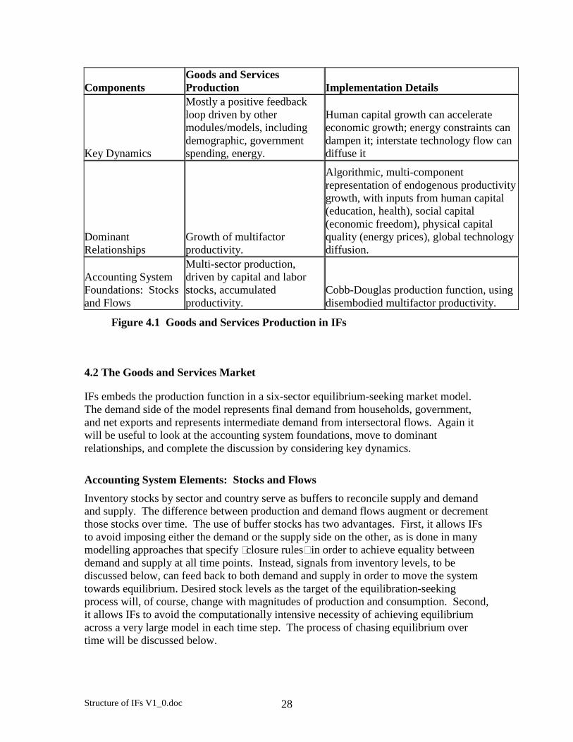
Components Goods and Services Production Implementation Details

Key Dynamics

Mostly a positive feedback loop driven by other modules/models, including demographic, government spending, energy.

Human capital growth can accelerate economic growth; energy constraints can dampen it; interstate technology flow can diffuse it


Growth of multifactor productivity.

Algorithmic, multi-component representation of endogenous productivity growth, with inputs from human capital (education, health), social capital (economic freedom), physical capital quality (energy prices), global technology diffusion.


Multi-sector production, driven by capital and labor stocks, accumulated productivity.

Cobb-Douglas production function, using disembodied multifactor productivity.

Figure 4.1 Goods and Services Production in IFs

4.2 The Goods and Services Market

IFs embeds the production function in a six-sector equilibrium-seeking market model. The demand side of the model represents final demand from households, government, and net exports and represents intermediate demand from intersectoral flows. Again it will be useful to look at the accounting system foundations, move to dominant relationships, and complete the discussion by considering key dynamics.

Accounting System Elements: Stocks and Flows

Inventory stocks by sector and country serve as buffers to reconcile supply and demand and supply. The difference between production and demand flows augment or decrement those stocks over time. The use of buffer stocks has two advantages. First, it allows IFs to avoid imposing either the demand or the supply side on the other, as is done in many modelling approaches that specify “closure rules” in order to achieve equality between demand and supply at all time points. Instead, signals from inventory levels, to be discussed below, can feed back to both demand and supply in order to move the system towards equilibrium. Desired stock levels as the target of the equilibration-seeking process will, of course, change with magnitudes of production and consumption. Second, it allows IFs to avoid the computationally intensive necessity of achieving equilibrium across a very large model in each time step. The process of chasing equilibrium over time will be discussed below.


Dominant Relationships The importance of the production function has already been emphasized, and it is no less important in the larger equilibrium-seeking goods and service market representation than in the production sub-system itself. What other relationships are most important in the goods and service market? With respect to the values that motivate the model, including the pursuit of human development, fairness within social relations and therefore some measure of equity, and environmental sustainability, and with respect to the long-term dynamics of the model, the most important relationships are those around consumption by government and especially households. Total household consumption is tied directly to income, which is in turn based on labor earnings, returns on capital, and transfer payments (all of which will be discussed in connection with the social accounting matrix). Ideally IFs should represent consumption based on something like the permanent income hypothesis, linking it to age structures as well as income. At this point it does not do so. Perhaps even more importantly for long-term analysis, it would be useful to step back from a focus on consumption to a focus on broader household utility, including time budgets that recognize trade-offs between employment and leisure. IFs does not currently have such a representation, but should develop one. The model does make the household division of income between consumption and savings responsive to an interest rate index, which is in turn responsive to the overall balance between production and consumption sides of the model. This formulation allows household consumption to adjust somewhat with, for example, the increasing share of government in most economies, to be discussed below. Consumption by sector is also an important relationship, in part because it determines the balance between more and less materially intensive sectors. IFs uses a linear expenditure system (LES) formulation that recognizes in the Engel parameters the distinctions between inferior and superior goods and relies on those parameters to shift household consumption away from food and manufactures and towards services with higher income.9 IFs has a formulation for governmental demand that recognizes Wagner’s Law, the propensity for the size of government as a share of the economy to grow over time. The foundation of the formulation is a cross-sectionally estimated relationship between GDP per capita (PPP) and government share of the economy. There has, however, been an upward shift of that function over time and IFs adds such a shift to the representation.

9 Although this is a standard approach, it may be that for longer-term modeling it would be useful to consider more of a goal-seeking formulation, representing target distributions of consumption across sectors at different income levels. The disadvantages of relying on a fixed coefficient-driven system like the LES for long-term modeling are that they may not be very transparent or even stable in their behavior as the system moves a long distance from initial conditions.


The formulation has a cap built in to protect the system from government take-over of the entire economy, but a more sophisticated saturation of government share would be desirable. With respect to intersectoral flows or intermediate demand, IFs uses a dynamic mechanism to change technological matrices with GDP per capita level and therefore to represent the impact on intermediate demand of changing technological levels with development. It bases those shifts on a set of technological matrices at different levels of development that come from data of the late 1990s. Thus the model does not capture the inevitable advance of production technology over time by positing future technological matrices. Doing so would be a potentially important step in showing dematerialization. With respect to total demand placed upon sectors of production, however, the shift of technology over time is relatively insignificant compared to the impact of total household and government consumption and the sectoral constitution of them. Many, if not most multi-country economic models represent trade bilaterally, but IFs uses a pooled approach. The bilateral representations, using something like an Armington formulation to build in inter-country biases and inertia in their change, can be valuable for models in which trade flows are used as a foundation for inter-country political relationships or in which they substantially affect development prospects. IFs looks to overall levels of trade as portions of the economy and to trade balances for the primary effects in both of these areas. The use of pooled trade is computationally very efficient. Key Dynamics The pursuit of equilibrium significantly drives the shorter-term dynamics of the model. As indicated earlier, the economic sub-model makes no attempt through iteration or simultaneous solution to obtain exact equilibrium at any time point. Kornai (1971) and others have, of course, argued that real world economic systems are not in exact equilibrium at any time point, in spite of the convenience of such assumptions for much of economic analysis. Moreover, the SARUM global model (Systems Analysis Research Unit, 1977) and GLOBUS (Hughes, 1987) use buffer systems similar to that of IFs with the model "chasing" equilibrium over time.

The central equilibrium problem that the module must address is maintaining balance between supply and demand in each of the sectors of the model. IFs relies on two principal mechanisms to assure equilibrium in each sector: price-driven changes, mediated by elasticities, in domestic demand and trade; and stock-driven changes in investment by destination (so as to avoid a 2-year time delay in the response of investment and because of its recursive structure, IFs uses stocks instead of prices to drive changes in investment patterns).

Equilibrium-seeking mechanisms within IFs, including these two, are normally handled by an adjustment mechanism that is sometimes called a PID controller. A PID-driven adjustment process responds proportionately to the integral of the error (the stock discrepancy) and to the derivative of the error (the change in stock term). For more information about PID controllers, which come from engineering, see the books by


Chang (1961) and by Mishkin and Braun (1961). An early version of this adjustment mechanism was developed by Thomas Shook for the Mesarovic-Pestel modeling project.

The production function and the rates of growth it generates are the primary drivers of the longer-term dynamics of the goods and services market. Consumption patterns influence these dynamics at the margin, as sectoral shifts occur. These shifts can even lead to some degree of immaterialization of consumption over time (as demand shifts from manufactures to services) and therefore to some reduction in material intensities of economies. Yet the income of households is fundamentally tied to the value added by labor in production, and therefore total consumption derives essentially from the production function. The representation of broader household utility, introducing more trade-off between work and leisure, would add an additional element of impact on long-term dynamics from the consumption side; yet given the relatively small contribution of labor to the total production function, even that representation would largely leave the accumulation of technical change and of capital stock in charge of long-term economic model dynamics.

Components Goods and Services Markets Implementation Details

Key Dynamics

Dynamic computable general equilibrium model (CGE) structure pursues target inventory levels; changes in prices provide signals to production, consumption, trade, and investment.

Equilibration uses PID controller and is not tuned to create standard cycles.


Production from detailed formulation. Total government and household spending tied to income levels. Sectoral consumption function is price responsive. Trade is price, exchange-rate responsive.

Division of consumption uses LES. Trade uses pooled, not dyadic approach.


Multi-sector supply and demand, using inventories as balancing stocks; production and imports increment stocks while consumption and exports decrement them.

Six sectors using dynamic IO matrix.

Figure 4.2 Goods and Services Markets in IFs

4.3 The Social Accounting Matrix

Just as the production function is imbedded in the representation of the goods and services market, the goods and services market is imbedded in the larger system of the social accounting matrix. The social accounting matrix (SAM) tracks and dynamically represents the financial stocks (assets and liabilities) and flows associated with key agent-


classes. The SAM makes it possible to investigate the impact of domestic and interstate financial transfers and opens us many lines of analysis. For example, the SAM representation ties spending on pensions to the aging of the population; representation of the inherent trade-offs between government transfers related to aging and those related to other welfare concerns has implications for income distribution. Similarly, relationships within the SAM facilitate analyses around issues such as those of the Millennium Development Goals, including poverty reduction and the potential importance of a global compact. Accounting System Foundations: Stocks and Flows Figure 4.3, from IFs, shows the general character of the Social Accounting Matrix. Richard Stone is the acknowledged father of social accounting matrices, which emerged from his participation in setting up the first systems of national accounts or SNA (see Pesaran and Harcourt 1999 on Stone’s work and Stone 1986). Many others have pushed the concepts and use of SAMs forward, including Pyatt (Pyatt and Round 1985), Khan (1998) and Thorbecke (2001). It is fitting that the 1993 revision of the System of National Accounts by the United Nations has begun explicitly to move the SNA into the world of SAMs.

Figure 4.3 The Rolled-Up Social Accounting Matrix of Flows in IFs: Flows

Many of the cells in the matrix above are roll-ups or aggregates of more detailed elaborations within the SAM. For instance, the matrix in Figure 4.4 shows the detail of intersectoral flows that lies below the cell in the upper left of Figure 4.3.


Figure 4.4 A Disaggreated Cell of the Rolled-Up SAM

What the SAM adds to the goods and service market is addition of representation of financial flows among agent classes to those directly tied to the production, exchange, and consumption of goods and services. In Figure 4.3, the first column and the first row are financial flows already in the goods and services market. For instance, the two cells identified as flows to firms and households from sectors are the value added to production by firms and households (the sum of which is GDP) and are the financial return to those agent classes from the production activity. Similarly, the flows from government to sectors are the direct purchases of goods and services by government. The remaining cells are additions by the SAM to goods and service markets and are mostly flows among agent classes. For instance, governments receive taxes from households and firms, make transfer payments back to households, pay interest on debts to the rest of the world or provide foreign aid to other countries, etc. It is the tracking of these additional financial flows, many of which are essential to understanding the leverage that human action has with respect to changing patterns of growth or affecting income distributions, that the SAM adds. The approach of IFs with respect to SAMS builds on earlier work, but also extends that work on five fronts (with substantial work yet to be done on most fronts):

The universality of the SAM representation. Most SAMS are for a single country or a small number of countries or regions within them. IFs has created a procedure for constructing relatively highly aggregated SAMs from available data for 164 different countries, relying upon estimated relationships to fill sometimes extensive holes in the available data. Jansen and Vos (1997: 400-416) refer to such aggregated systems as using a “Macroeconomic Social Accounting Framework.” Each SAM has an identical structure and they can therefore be easily compared or even aggregated (for regions of the world).

The connecting of the universal set of SAMs through representation of the global financial system. Most SAMs treat the rest of the world as a residual category, unconnected to anything else. Because IFs contains SAMs for all countries, it is important that the rest-of –the-world categories are mutually


consistent. Thus exports and imports, foreign direct investment inflows and outflows, government borrowing and lending, and many other inter-country flows must be balanced and consistent.

The representation of stocks as well as flows (see Figure 4.5). Both domestically and internationally, many flows are related to stocks. For instance, foreign direct investment inflows augment or reduce stocks of existing investment. The total debt of governments affects government taxation and spending, just as the wealth of households affects their spending (and, were time budgets added for households, might affect decisions about work versus leisure). Representing these stocks is therefore important from the point of view of understanding long-term dynamics of the system because such stocks, also including aggregate levels of portfolio investment, IMF credits, World Bank loans, reserve holdings, and domestic capital stock invested in various sectors, generate flows that affect the future. Specifically, the stocks of assets and liabilities will help drive the behavior of agent classes in shaping the flow matrix. The representation of stocks within IFs is not yet very fully developed (although it is more extensive than indicated in Figure 4.5).

Embedding the SAM structure within a long-term global model. The economic module of IFs has many of the characteristics of a typical CGE, but the representation of stocks and related agent-class driven behavior in a consciously long-term structure introduces a quite different approach to dynamics. Instead of elasticities or multipliers on various terms in the SAM, IFs seeks to build agent-class behavior that often is algorithmic rather than automatic. To clarify this distinction with an example, instead of representing a fixed set of coefficients that determine how an infusion of additional resources to a government would be spent, IFs increasingly attempts partially to endogenize such coefficients, linking them to such longer-term dynamics as those around levels of government debt and changing age-structure of the population. Much of this kind of representation is in very basic form at this stage of model development, but the foundation is in place.

The inclusion of a number of other submodels relevant to the analysis of longer-term forecasts. As discussed above, efforts have been made to provide a dynamic base for demographic and economic drivers of the IFs model such that forecasts can be made well into the 21st century. In addition the partial equilibrium models for agriculture and energy, to be discussed in subsequent chapters, are linked into the overall economic model.


Figure 4.5 The Social Accounting Matrix System in IFs: Stocks


The dominant relationships of the SAM system are those that describe basic patterns, always changeable by users, of the flows from and to agent classes. For instance, Figures 4.6 and 4.7 show typical base-line patterns for change in public pension transfers/spending and direct government consumption (health, education, military, etc.) as a function of GDP per capita. These are bases for formulations of such transfers and spending that have considerably more complexity. For instance, pension spending is tied to the growth of the aged population and military spending is responsive to an action-reaction dynamic with other countries.


y = 2.8424Ln(x) + 0.5227R2 = 0.5335

-4

-2

0

2

4

6

8

10

12

14

16

0 10 20 30 40 50

GDP/Capita (PPP) in $1,000

Pu

blic

Pen

sio

n S

pen

din

g a

s P

erce

nt

of

GD

P

Figure 4.6 Government Spending on Pensions as Function of GDP/capita (PPP)

y = 1.8509Ln(x) + 12.697R2 = 0.1277

0

10

20

30

40

50

60

0 10 20 30 40 50

GDP/Capita (PPP) in $1,000

Go

vern

men

t C

on

sum

pti

on

as

Per

cen

t o

f G

DP

Figure 4.7 Government Consumption Share as Function of GDP/capita (PPP)

Figure 4.8 shows the basis for representation of flows from another agent, specifically lending from the World Bank. Again, there are substantial additional elements of the full formulation, including those that tie global totals of Bank lending to the asset base of the institution.


y = 28.669x-1.4303

R2 = 0.5868

0

20

40

60

80

100

120

0 10 20 30 40 50

GDP per Capita at PPP, Thousand Dollars

WB

Lo

ans

Rec

eive

d, P

erce

nt

of

GD

P

Figure 4.8 World Bank Lending as a Function of GDP per Capita

In addition to an extensive representation of the relationships behind intra-country flows such as those from and to government and of flows around the World Bank, there are extensive interstate flows such as foreign direct investment (FDI), portfolio investment and worker remittances. It is important, however, to understand that IFs is not intended to be a model of shorter-term financial systems in which such overshoots or collapses will occur, but rather of longer-term patterns and unfoldings. The latter orientation frames the way in which IFs represents actor-class behaviour, as illustrated by FDI.

Firms are primarily in charge on both ends of foreign direct investment. In general, of course, the pattern is likely to be that firms direct FDI from relatively capital-rich countries to relatively capital-poor ones. Figure 4.7 below reinforces that presumption by showing the patterns found in the IFs database (using FDI flow data from the World Bank’s World Development Indicators). The less steeply-sloped line is the relationship between GDP per capita at PPP and the inflows of FDI as a percentage of GDP. The more steeply-sloped line is the relationship between GDP per capita at PPP and the outflows of FDI as a percentage of GDP. Both lines are upward sloping and, in fact, countries are simultaneously larger sources and targets of investment, even relative to GDP, as they develop. Yet, roughly speaking, countries are net recipients until GDP per capita is somewhat above $20,000 and net sources thereafter.

IFs recognizes that these patterns will not be universal. Thus the algorithm that determines investment outflows is one that builds in the historic pattern of an FDI source, but that assumes convergence over long periods of time, such as a century, towards the generic pattern. The same is true for recipients. It would probably be reasonable to posit that both lines would shift to the right over time as the average per capita levels of global GDP increase, although such a presumption does not exist in the model at this time.


GDP/Capita (PPP) Versus FDIStock Inflows Over GDP (2000)

GDP/Capita (PPP) Versus FDIStock Outflows Over GDP(2000)

0.0

0.1

0.2

0.3

0.4

0.5

0 10 20 30 40

Figure 4.9 FDI Inflows and Outflows as a Function of GDP per Capita

In addition to the relative behavior of firms in states across the system, another behavioral issue is the overall pattern of increase or decrease in FDI flows relative to the size of the global economy. Over the last several decades FDI has grown steadily as a portion of the global capital stock and global economy. Economic historians are, however, quick to point out that the turn of the 20th century was a period of enhanced globalization of capital, and that those flows then retreated for most of the 20th century before advancing again. And this century has already seen retreats relative to the year 2000. Thus the base case presumption built into IFs, based roughly on patterns of the late 1990s, is of growth in FDI flows at a rate that exceeds economic growth but that convergences towards GDP growth by 2010.

These relationships around the SAM are only very selectively illustrative. See Hughes and Hossain 2003b for full elaboration of the SAM.

Key Dynamics

In contrast to the production function and even to the representation of consumption, specific relationships in the social accounting matrix often do not to have large direct implications for the longer-term dynamics of the model. In fact, many of them will, via transfers, primarily shift well-being across actor classes. Yet any such shifts will, of course, affect dynamics in part through the impact they might have on productivity. For instance, shifts of government spending to education and health will have such affects; movements of funds from more to less developed countries will influence growth prospects in each. Some productivity-path effects, such as increased spending on R&D, could potentially be quite large.

Because the earlier discussion elaborated the production-function linked dynamics, this discussion will focus on dynamics more specific to the SAM. Most of those help maintain accounting balances and thereby constrain interactions of agent classes and financial trade-offs faced by them. Not surprisingly, the key function of Social ACCOUNTING Matrices is accounting, not dynamics. Most of the dynamics specific to the SAM are goal-seeking or equilibrating, and implementation of them uses the PID controller mechanism described earlier for the goods and services market. Specifically,


many of the relationships set target values for dynamics around asset and liability levels, often represented as a portion of GDP.

For instance, Figure 4.10 shows a cross-sectional relationship of government debt level as a portion of GDP as a function of the per capita level of GDP. The relationship is very weak, but provides a benchmark for long-term levels of debt. IFs actually uses the lower of initial debt ratios and the value from the function as the long-term target level for specific countries. When debt exceeds the target level, expenditures are cut and revenues rise.

y = -15.289Ln(x) + 83.955R2 = 0.1794

0

50

100

150

200

250

300

0 10 20 30 40 50

GDP per Capita at PPP (Thousand Dollars)

Go

vern

men

t D

ebt

as P

erce

nt

of

GD

P

Figure 4.10 Government Debt Levels as a Function of GDP per Capita (PPP)

One of the most important fiscal constraints for many countries is that around the stock of international debt, as affected by the flows in current account balances. Figure 4.11 shows another cross-sectional relationship that provides a general long-term constraining target level for external debt within IFs.


y = -0.3668Ln(x) + 1.1822R2 = 0.2776

-1

0

1

2

3

4

5

0 5 10 15 20 25 30

GDP per Capita at Purchasing Pow er (Thousand Dollars)

Inte

rnat

ion

al D

ebt

as R

atio

to

GD

P

Figure 4.11 International Debt Levels as a Function of GDP per Capita (PPP)

Representations of agent-class behavior and undertaking of policy analyses benefit greatly from such goal-seeking formulations. For instance, the calculations of stocks of debt for recipient countries as well as flows of lending from the World Bank provides the foundation for representing repayment flows to the Bank; the long-term implications of modeling two-way flows with stock-driven loan repayment tends to be very different from the representation of short-term one-way flows. Components Finance Implementation Details

Key Dynamics

Setting of target (or maximum) levels of assets and liabilities for agent-classes. Goal-seeking equilibration for assets and liabilities of agent-classes, e.g. domestic equilibration around debt levels of government. International equilibration around international debt levels.

Many target values are based on cross-sectional relationships with PID controllers for flows. No equilibration around household debt or wealth at this time.


Representation of agent-class behavior around flows. Includes World Bank lending across countries and to various target uses. Heavily algorithmic formulations.


Social Accounting Matrices (SAMs) for flows, tied to underlying asset/liability stock representations.

Representations of households (skilled/unskilled), governments, firms and rest of world (ROW). ROW representations, balanced globally, include FDI, equity, aid, and IFI flows.

Figure 4.8 Modeling the Social Accounting Matrix System in IFs


5. Energy The energy submodel of IFs is a dynamic, partial equilibrium-seeking model that represents resources, production, consumption and trade of energy in physical units and computes monetary values that are needed to link such calculations to the monetary representations in the general equilibrium-seeking economic model. IFs models the energy production systems for each of its geographic countries/regions in terms of resources and production of oil, natural gas, coal, hydroelectric power, nuclear, other renewable, and unconventional or synthetic hydrocarbons. The model uses production functions that depend on capital and technological sophistication, but not labor. The demand side computes aggregate energy demand as a function of GDP levels and prices. Energy trade is modeled via a pooled formulation of total energy, rather than bilaterally or by energy type. Production, consumption, and exchange of energy come together in the representation of an energy market that relies on changes in inventory stocks and price signals to pursue equilibrium over time. The energy model can usefully be understood in terms of (1) accounting foundations that represent stocks, with particular attention to energy resources and reserves, and flows, (2) the formulations of dominant relationships that determine behavior, and (3) approaches to key dynamics that characterize the integrated system. As in the discussion of the economic model, it is useful to build up to the full energy model in three steps. The first step considers fossil fuel energy resources. The second step broadens attention to production of energy. The third step broadens attention further to the consumption and exchange of energy, that is to a full partial equilibrium market for energy. The rest of this chapter considers each of these elements in turn.

5.1 Energy Resources

Accounting System Foundations: Stocks and Flows The forms of energy that are dominant today and that will most likely dominate energy supply for a few more decades are fossil fuels. It is impossible to think seriously about the long-term future of fossil fuels in the energy system without thinking about the resource base. What is often called the McKelvey Box is an excellent conceptual scheme for understanding energy resources such as those of oil, natural gas, and coal. It uses two dimensions, discovered/undiscovered and commercial/sub-commercial to distinguish reserves (the discovered and commercial) as a subset of in-earth resources. The argument is that different price levels and extraction technologies interact to determine what is commercial.


The U.S. Geological Survey, where Vincent McKelvey was director from 1971 to 1978, now uses a version that the contemporary energy industry and IFs have adopted. Reserves are essentially the same concept (discovered and commercially viable today), but there are two different concepts, corresponding to the two dimensions, that increment the potential stocks available for production over time. The first is undiscovered resources and the second is potential reserve growth (expansion of the commercially viable share of currently discovered resources). Periodic assessments by the USGS (most recently in 2000) provide analyses by basin and country of undiscovered resources of oil, gas, and natural gas liquids with different probability levels of their ultimate discovery. Outside of the U.S., however, they do not provide country-specific estimates of potential reserve growth, providing only a global estimate.10 IFs therefore aggregates the two reserve-expansion categories (quadrants 2 and 3 in Figure 5.1) into a single category of total potential resources, encompassing known and viable reserves (quadrant 1) as a subcategory. There are two key flows associated with this conceptualization of two stocks, reserve increase via discovery or reserve growth (movement from quadrants 2 or 3 into quadrant 1) and production, which decrements reserves from quadrant 1. Discovered Undiscovered (often

estimated with different probabilities of discovery, such as 95%, average estimate, 5%.

Commercially Viable 1. Reserves – discovered and commercially viable with current prices and technology

2. Source of new discoveries that are commercially viable

Not Viable (sometimes subcategorized as marginal and sub-marginal)

3. Source of reserve growth – discovered earlier, but added to reserves because of new technology or price changes

Figure 5.1 McKelvey’s Box of Reserve/Resource Classifications as Conceputalized in IFs.

10 In private conversation with Ronald Charpentier of the USGS Assessment Team, he affirmed that a reasonable way in which to divide the global estimate of potential reserve growth across countries was in the same proportions as undiscovered resources. Although the approach of the World Energy Council with respect to coal resource data is not quite as elaborate, it may be the best available and those data are being used by IFs with the same general conceptual and modeling approach.


Dominant Relationships The key relationships with respect to flows are, as indicated, production and reserve discovery/growth. Both are critical to long-term dynamics. The next section treats production. Discoveries/reserve growth are forecast by a relationship that sets global discovery/reserve growth rates, and rate of change in those rates, so as to generate roughly the recent reserve expansion/contraction pattern globally. Country-specific portions of the global discoveries/reserve growth are allocated proportionally to countries based on their share of potential global discovery/reserve growth. As cumulative discoveries/reserve growth approach the maximum potential discoveries/reserve growth, the global rate is dampened. Except in countries/regions that have reserve levels that are already significantly constraining production (like the U.S. oil reserves), the model is not highly sensitive to this particular set of dynamics, but rather to the total estimates of potential discoveries/reserve growth. The more critical relationship is the production function itself, to which the discussion will soon turn. Key Dynamics The representation of stocks and flows of resources described above, in combination with the production function to be elaborated below, produces over time another famous pattern, the Hubbert’s (sometimes Hubbert) Curve of resource production. M. King Hubbert, while a geologist at Shell Oil in 1956, argued that the life-cycle production patterns for limited resources resembled the bell-shaped curve in Figure 5.2

Figure 5.2 Hubbert’s Curve. From Energy and Power, A Scientific American Book, 1971, pg 39; downloaded from http://www.hubbertpeak.com/hubbert/.

http://www.hubbertpeak.com/hubbert/energypower/


The total area under the bell-shaped curve cannot exceed the ultimately discoverable and producible resource base and the key debate about dynamics around oil and natural gas concerns how fast the curve will rise and when the peak will occur. Hubbert’s approach gained a great deal of credibility when he forecast that the U.S. would reach the top of its own production curve for the lower 48 states in 1970, a prediction that was almost exactly correct. The portrayal of the global curve in Figure 5.2, released in 1971, was obviously much further from the mark and their remains substantial debate about when the global peak will be reached (reviewed in Hughes 2004, March)

Components Energy Resources Implementation Details

Key Dynamics

Resource exhaustion ultimately constrains replenishment of fossil fuel reserves.


Rates of discovery and rates of production.

Algorithmic formulations determine discovery rates and larger module determines production.


Non-renewable resources use "McKelvey's Box" with discoveries/extensions increasing reserves (a stock) and production decrementing them. Fossil fuels are oil, gas, coal.

Figure 5.3 Energy Resources in IFs

5.2 Energy Production

Accounting System Foundations: Stocks and Flows IFs uses a production function for energy that involves capital stock invested and a capital-to-output ratio (the former, divided by the latter, determines energy production in physical units, namely billion barrels of oil equivalent). Capital stocks are maintained by energy type, including renewable sources, but not by vintage, and capital stocks are not substitutable across energy types. Capital depreciates over time and the flow of new investment, allocated to the energy sector based in part on prices relative to costs (profits), are further allocated to capital by energy type in the same way. A second stock-like variable in the energy model is analogous to multifactor productivity in the economic model. It is the contribution of technology via the reduction of capital costs per unit of energy output. In contrast to the broader economic model, however, the rate of technological advance for each energy type is specified exogenously.


Dominant Relationships The key driver of energy production, even more than capital stocks, is the capital-to-output ratio. This is because global economies have sufficient capital to meet their energy needs. But the capital-to-output ratio effectively determines the relative cost of different forms of energy in the mix. The capital-to-output ratio itself carries information about two stocks. The first element in the calculation of capital-to-output ratios, similar to that of multifactor productivity in the economic model, is the cumulative reduction in capital costs for energy production, driven by the exogenously specified growth rate of that technological advance. The second element in the calculation is the ratio of remaining resources to initial resources. As this ratio becomes smaller, it increases the capital-to-output ratio. Whether the amount of capital needed to produce a given unit of energy is decreasing or increasing depends on whether the reductions driven by the technological-progress term are larger or smaller than the increases from the resource-depletion term. Key Dynamics Because the ongoing depletion of fossil fuels, notably oil and natural gas, ultimately creates rising capital costs in the production of those fuels, while there is limited global depletion of coal and there is potentially even less rapid global saturation in the use of some forms of renewable energy, the determination of the capital-to-output ratio ultimately shifts investment and therefore energy production from oil and gas to coal and/or renewables. Even renewable forms are not completely free from some dampening effect from “resources.” Good sites for hydropower are heavily depleted and there are presumably some upper limits to the use of windmills and photocells, although they are largely beyond the normal century-long horizon of the IFs model. Components Energy Production Implementation Details

Key Dynamics

Reserve depletion constrains production of fossil fuels, while technology change drives renewable costs and production.

Reserve/production ratio minimums implement reserve constraint.


For non-renewable energy forms, capital-output ratios fall with technology assumptions and rise as reserve/production ratios fall. For renewable energy forms capital-output ratios fall with technological assumptions. Investment levels respond to price/profit signals.

Largely algorithmic formulations. Technological assumptions mostly exogenous, but some learning by doing.


Capital stocks and capital/output ratios drive production of energy, by type.

Figure 5.4 Energy Production in IFs


5.3 Energy Markets

IFs embeds the energy production function in an equilibrium-seeking energy market model. The demand side of the model represents total demand of country-wide economies in physical energy units. The market model also represents exports and imports of energy, again in physical units (in a pooled approach not specific to energy type). The discussion will once again look at the accounting system foundations, move to dominant relationships, and complete the discussion by considering key dynamics.


Inventory stocks of energy by country, in physical units, serve as buffers to reconcile supply and demand. The difference between production and demand flows augment or decrement those stocks over time. The use of buffer stocks has the same advantages as in the economic model. First, it allows IFs to avoid imposing either the demand or the supply side on the other. That is, signals from inventory levels can feed back to both demand and supply in order to move the system towards equilibrium. Desired stock levels will, of course, change with levels of production and consumption. Second, it allows IFs to avoid the computationally intensive necessity of achieving equilibrium across the model in each time step.

Dominant Relationships In more substantially-elaborated energy models, energy demand is normally differentiated across at least industrial, residential, and transportation final uses. Within those categories of use models often make a distinction with respect to energy preferences (currently, transportation use demands primarily gasoline). Energy models also often differentiate between primary energy types (like oil, nuclear, or hydroelectric power) and intermediate forms such as electricity and the emergent hydrogen carrier. In IFs the demand side of the model has been greatly simplified to a single computation of total energy demand, to be compared to the sum of energy supplies from various forms. Energy trade is similarly simplified to billion barrels of oil equivalent, regardless of energy form. It is therefore not surprising that, beyond the production function described above, the dominant relationship in the representation of the energy market is the aggregate demand function. In IFs the size of GDP is the key driver of that function, with prices also entering into the formulation. The key difficulty with formulating this relationship is that estimation-based relationships are not very convincing. There is, for instance, a reasonable hypothesis in the literature that energy demand per unit of GDP follows a pattern called the environmental Kuznets curve (an inverted U-shaped curve that Kuznets first popularized when examining income distribution) as countries develop economically. According to this hypothesis, as


countries begin to develop economically, energy use per unit of the economy rises at first and then declines. The foundation of the hypothesis generally is the notion that economies go through an energy-intensive, relatively highly polluting industrial phase and then move into less energy intensive services.11 Figure 5.5 uses cross-sectional energy data to examine that hypothesis and shows that there is some evidence for it, but not a great deal. Moreover, the right-hand tail of the estimated relationship drops below zero, making it rather difficult to use in forecasting. Most importantly, however, this curve is purely an artifact of the inclusion in the analysis of a number of developing countries for which missing data (nulls) were treated as zero (no energy consumption). Such treatment is obviously inappropriate.

y = -9E-06x2 + 0.0002x + 0.0033R2 = 0.0349

-0.01

-0.005

0

0.005

0.01

0.015

0.02

0.025

0.03

0 10 20 30 40 50


En

erg

y C

on

sum

pti

on

per

Do

llar

of

GD

P (

BB

OE

)

Figure 5.5 Energy Consumption Intensity as a Function of GDP per Capita (The Kuznets Curve) – Data from 1995.

Figures 5.6-5.8 move to more serious analysis of energy data, omitting null values. They show relationships between GDP per capita and energy use per unit of GDP in, respectively, transportation, residential, and industrial applications. Note that the best fitting curve for transportation applications is a power curve, while those for residential and industrial applications are exponential. All these are downward sloping across all levels of GDP per capita, contradicting the notion of the Kuznets curve.

11 An accessible review is by Lizzie Candia, “Does the Environmental Kuznets Curve Explain How a Growing Economy Can Achieve Better Environmental Quality?” at http://www.dundee.ac.uk/cepmlp/car/html/car7_article8.pdf. She cites G. Grossman and A. Krueger, “Economic Growth and the Environment, “ Quarterly Journal of Economics 110, 353-377 (1995).


y = 0.0008x-0.2458

R2 = 0.182

0

0.0005

0.001

0.0015

0.002

0.0025

0.003

0.0035

0 10 20 30 40 50


Tra

nsp

ort

atio

n E

ner

gy

Use

per

GD

P

Un

it (

BB

OE

/Bill

ion

Do

llars

)

Figure 5.6 Transportation Energy Consumption Intensity as a Function of GDP per Capita – Data from 1999.

y = 0.0013e-0.0867x

R2 = 0.4122

0

0.002

0.004

0.006

0.008

0.01

0.012

0.014

0.016

0 10 20 30 40 50


Res

iden

tial

En

erg

y C

on

sum

pti

on

p

er U

nit

of

GD

P (

BB

OE

/Bill

ion

Do

llars

)

Figure 5.7 Residential Energy Consumption Intensity as a Function of GDP per Capita – Data from 1999.


y = 0.0009e-0.0356x

R2 = 0.1236

0

0.002

0.004

0.006

0.008

0.01

0.012

0.014

0.016

0 10 20 30 40 50


Ind

ust

rial

En

erg

y C

on

sum

pti

on

per

G

DP

Un

it (

BB

OE

/Bill

ion

Do

llars

)

Figure 5.8 Industrial Energy Consumption Intensity as a Function of GDP per Capita – Data from 1999.

In Figures 5.9 and 5.10, the analysis returns to energy use summed across use categories and the figures show, respectively, power and exponential formulations. Interestingly, the estimation summed across the three usage categories is stronger than that within any of the three, providing some additional support for the model’s reliance on aggregated energy demand.

y = 0.0051x-0.5189

R2 = 0.4487

0

0.002

0.004

0.006

0.008

0.01

0.012

0.014

0.016

0.018

0.02

0 10 20 30 40 50


Su

mm

ed U

se b

y T

ype

per

GD

P U

nit

(B

BO

E/B

illio

n D

olla

rs)

Figure 5.9 Summed Transportation, Residential, and Industrial Energy Consumption Intensity as Power Function of GDP per Capita – Data from 1999.


y = 0.0036e-0.0575x

R2 = 0.443

0

0.002

0.004

0.006

0.008

0.01

0.012

0.014

0.016

0.018

0.02

0 10 20 30 40 50


Su

mm

ed U

se b

y T

ype

per

GD

P U

nit

(B

BO

E/B

illio

n D

olla

rs)

Figure 5.10 Summed Transportation, Residential, and Industrial Energy Consumption Intensity as Exponential Function of GDP per Capita – Data from 1999.

The power formulation has a slightly (trivially) higher r-squared. The exponential formulation does not, however, have the steep downward slope on the left-hand tail. Because data for developing countries are not always trustworthy, there is an argument to be made for not building such a steep slope into our formulation based on the impact of a small handful of relationship outliers. At the same time, however, the power curve has a much flatter shape above $30,000 per capita. Experience based on testing the exponential curve in the model shows that the substantial rate of decline leads to rates of decrease in energy demand that are totally inconsistent with historic experience. In short, the power curve appears to be better for higher levels of GDP per capita, while the exponential curve appears better for lower levels of GDP per capita.

Under such circumstances, what is a modeler to do? One option is to use a combination of the two. Figure 5.11 shows a simple version of what is called a table function, a function constructed via linear segments in order to provide the rough shape of a function that is not easy to specify analytically. The pattern in Figure 5.11 has an initial segment that is something of a compromise between the power and exponential formulations and a secondary segment that is closer to the power formulation. IFs uses this basic approach for the representation of energy demand, but because of the special importance of this function, it is available for change by the user.


GDP/Capita (PPP) VersusEnergy Demand per GDPDollar (1995)

0.000

0.001

0.002

0.004

0.005

0.006

0 20 40 60 80 100

Figure 5.11 A Table Function for Energy Demand

There is another possible approach to forecasting of energy demand to which IFs could possibly switch and which is used by Shell (2001) in some of its forecasting. That is to look at per capita energy demand as a function of GDP per capita, as in Figure 5.12. The per-capita approach is used in forecasting food/calorie consumption, to be described in the next chapter. The r-squared is not as high, but the form of the function is somewhat better behaved.

y = -3E-05x2 + 0.0024x - 0.0012R2 = 0.3829

-0.05

0

0.05

0.1

0.15

0.2

0.25

0 10 20 30 40 50


To

tal C

om

mer

cial

En

erg

y C

on

sum

pti

on

per

Cap

ita

(199

5)

Figure 5.12 Energy Demand per Capita as Function of GDP per Capita

Continuing with the current formulation, however, we also know that prices should affect energy demand. Cross-sectional estimation is not, however, very helpful. For instance, adding gasoline prices to estimation of the above relationships between GDP per capita and transportation energy use does not statistically improve the relationship. Yet analysis in the 1970s and 1980s, when world energy prices rose sharply and then fell, definitively showed that the demand elasticity effects were larger than expected and, in fact, demand proved more responsive than did supply. IFs adds an energy price elasticity to the demand relationship drawing upon other studies and tuning of behavior to parameterize it.


Still further, we know that there has been a long-term decrease in energy demand per unit of GDP related to technological improvements. Nakiãenoviã, Grübler, and McDonald (1998: 6) suggest that the historic pattern is for annual declines of 1% in the growth of energy demand relative to GDP. They use a range of 0.8% to 1.4% for their forecasts and a similar practice has appeared in the simulations of Shell, the International Energy Agency, and essentially all other forecasting groups of note in the energy area. The IFs model includes a parameter of technological advance reducing energy demand in the formulation that adds to the above income and price terms, essentially completing the current formulation of energy demand. Using this complete formulation, the forecasts of the IFs base case prove very comparable to those of other energy analysts (Hughes March 2004). Yet this, like all dominant relationships in the model, deserves regular attention. In particular, there is reason to question the proposition that energy demand will tend to grow at about 1% a year less than the GDP. Figure 5.13 shows that energy demand was growing in near lock-step with GDP in the U.S. from 1960 until the first oil shock of the 1970s. Since that time, the ratio has declined at a rate closer to 2% per year.12 In short, many of the formulations used by forecasters could be failing to truly distinguish price and price-independent technology effects.

1.0

1.1

1.2

1.3

1.4

1.5

1.6

1.7

1.8

1.9

2.0

2.1

Energy Demand per Unit of GDPUnited States

Year

19621966

19701974

19781982

19861990

19941998

Figure 5.13 Energy Demand per Unit of GDP in the U.S. Barrels of Oil Equivalent per Thousand Constant Dollars.

Figure 5.14 shows a similar pattern for OECD countries generally since 1971. But surprisingly, the pattern for non-OECD countries is very different, showing a marked

12 The energy data used in this figure and the others in this set come to the IFs project from the International Energy Agency via the World Resource Institute’s Earth Trends dataset.


increase in energy intensity of those economies. The two groupings together give rise to a global pattern of near stability in energy intensity.

0.0

0.5

1.0

1.5

2.0

2.5

3.0

3.5

Energy Demand per Unit of GDPNon-OECD Countries, OECD Countries, and the World

Year

19731976

19791982

19851988

19911994

1997

non-OECD OECD World

Figure 5.14 Energy Demand per Unit of GDP in OECD and non-OECD countries and in the World. Barrels of Oil Equivalent per Thousand Constant Dollars.

It is important to point out immediately that much of the energy data for non-OECD countries is quite poor, especially that which has been built up as the sum of transportation, industrial, and residential consumption, as these series have. Note in Figure 5.15 that the sequences for China and India, two critical countries, have major transients that carry forward to the non-OECD totals, above. Specifically, there are huge jumps in all types of energy consumption in China in 1980, in Chinese residential use in 1994, and in India industrial use in 1994. [Anwar – we need to work on the data here; such transients should not be affecting our analysis.]


1

2

3

4

5

6

7

8

9

10

11

12

Energy Demand per Unit of GDPChina and India

Year

19721975

19781981

19841987

19901993

19961999

China India

Figure 5.15 Energy Demand per Unit of GDP in China and India. Barrels of Oil Equivalent per Thousand Constant Dollars.

These statistical anomalies make Figures 5.16 and 5.17 questionable, but they are still provocative and deserve attention. Figure 5.16 shows three cross-sectional relationships like those of Figure 5.9, linking GDP per capita cross-sectionally to energy demand around the world with power functions in each of three years (1971, 1985, and 1999). Figure 5.17 does the same, using exponential functions.13 In both cases, the implication is that energy demand per unit of GDP has fallen over time in rich countries, but risen in poor ones. In these figures, India and China are only two points.

GDP/Capita (PPP) VersusEnergy Demand per GDPDollar (1971 Power)



0.0000

0.0008

0.0016

0.0024

0.0032

0.0040

0 10 20 30 40

Figure 5.16 Cross-Sectional Relationships Between GDP per Capita and Energy Intensity at Three Different Time Points: Power Functions.

13 Over time the relationships have tightened, probably indicating better data, as well as more globalized markets in energy and production technology. The r-squareds for the power relationship grew from 0.04 in 1971 to 0.14 in 1985 to 0.44 in 1999. Those with the exponential function grew from 0.04 to 0.20 to 0.44.


GDP/Capita (PPP) VersusEnergy Demand per GDPDollar (1971 Exponential)



0.0000

0.0007

0.0013

0.0020

0.0026

0.0033

0 10 20 30 40

Figure 5.17 Cross-Sectional Relationships Between GDP per Capita and Energy Intensity at Three Different Time Points: Exponential Functions.

So is it possible that the spread of industrialization globally has, in fact, shifted energy demand away from developed countries and towards developing ones, with some reduction in energy intensities occurring for OECD countries but not for non-OECD countries? If so, the presumption of 1% global improvement in energy efficiencies will need to be reviewed again when this dominant dynamic is revisited. [Anwar: we need to add a good series of total energy demand to the dataset – the one we took earlier from a WDI CD for total commercial energy consumption, through 1995, has many zeros in it – obviously energy demand cannot be 0. Let’s look to both WDI and WRI for options. We also need to look to other modeling/estimation efforts for their analyses of energy demand elasticities – probably build a table.] Key Dynamics The pursuit of equilibrium significantly drives the shorter-term dynamics of the energy model. Like the economic model, the energy model makes no attempt through iteration or simultaneous solution to obtain exact equilibrium at any time point. And as in that model the primary mechanisms for pursuing equilibrium are changes in relative energy prices, with feedback to the demand side directly and to the supply side through shifts of investment levels and patterns. PID controllers smooth the adjustment processes. Both production side and demand side influence the long-term dynamics of the module in important ways. Because demand price-elasticities and changes in efficiency in energy use are both substantial, they can shape long-term behaviour of the energy system as much as do production technologies. As indicated earlier, the production side determines the rate of movement from oil and natural gas to other energy forms and the production side therefore greatly influences overall price levels. There are several key linkages between the energy model and the broader economic model with its energy sector. The sum of energy production in the model is used to compute the gross production of the energy sector in the broader model, and both export and import levels similarly feed back to the economic model. Also, the changes in price levels in the energy model, linked as they are to changing cost structures, feed back to relative price changes in the economic model, as do inventory levels (stocks). Those help


give signals in the investment allocation of the economic model, providing the share of investment in energy back to the energy model where it is allocated across production types. Components Energy Markets Details

Key Dynamics

Short-term dynamics preserve balance between demand and supply; long-term dynamics can move relative prices, driven by a combination of supply- and demand-side forces.

Buffer stocks allow the system to chase equilibrium and provide signals to supply and demand sides. Physical production, consumption and trade override monetary calculations in economic goods and services model, which provides investment to energy model.


Production from its own module. Demand responds to economy size, income levels, and price signals. Trade responds to local demand/supply imbalances and price signals.

Trade is responsive to prices and algorithmic in balancing global exports and imports.


Inventory stocks drive price changes and signals for equilibration.

Multi-energy-type model with production capacities by energy type and aggregated energy demand and trade. Fossil fuels are oil, gas, coal. Renewables are nuclear, hydro, and other renewables.

Figure 5.18 Energy Markets in IFs.


6. Agriculture The agricultural submodel of IFs is a dynamic, partial equilibrium-seeking model that represents land use, yield and production, consumption and trade of agricultural commodities for food and non-food use in physical units and computes monetary values that are needed to link such calculations to the monetary representations in the general equilibrium-seeking economic model. For each of its geographic countries/regions IFs represents land devoted to crops, grazing, forest, urban or other built uses, and an other/residual category. IFs models the agricultural production systems of crops and meat/fish. The agricultural model uses production functions that depend on land, capital, labor and technological sophistication. The demand side computes aggregate calorie demand as a function of population, GDP/capita levels and prices. Production, consumption, and exchange of agricultural commodities come together in a market representation that relies on changes in inventory stocks and price signals to pursue equilibrium over time. It is useful to portray the agricultural model in three steps. The first step involves consideration of land use. The second step broadens attention to production of agricultural commodities. The third step broadens attention further to the consumption and exchange of agricultural commodities, that is to a full partial equilibrium market. The rest of this chapter considers each of these elements in turn, looking in each case at accounting foundations, dominant relationships, and key dynamics.

6.1 Land Use

Until roughly the 1950s, most expansion of agricultural production globally was tied to expansion of area cultivated. Since that time, most production growth has come from rising yields per hectare of land. Nonetheless, changing land area remains of critical importance to the food system. Land use, especially contraction or expansion of forest area in trade off with crop and grazing land, is also a critical element of environmental systems, to be discussed in the next section of this report. Accounting System Foundations: Stocks and Flows The United Nations Food and Agricultural Organization (FAO) is the primary source of nearly every type of data related to agricultural systems. With respect to land use, it provides time series data on the portions of each country’s land in arable and permanent cropland (also tracking the two components separately), in permanent pasture, in forests and woodlands, and in other use. Another series tracks irrigated agricultural area. Somewhat surprisingly, the FAO has not historically tracked urban and built land as a portion of the “other use” category. Because movement of land from other categories to that one is one of the important dynamics of human land use systems, the IFs project uses data from the World Resources Institute Earthtrends project to separate out urban and built land from the broader “other” category (see Loveland et al 2000). To summarize,


the land categories in IFs are cropland, grazing land (permanent pasture), forest (with woodlands), urban (and built), and other. Over time the stocks of land in each category can shift significantly as hectares of land flow to other uses. The primary flows in recent decades have been into cropland, grazing area, and urban/built area, and out of forests, cropland, and grazing area. Dominant Relationships There are two dominant relationships in the determination of movement/flows of land from one use to another. The first is growth in urban/built usage of land and the second is conversion of land from other uses into cropland. This discussion focuses on the first of the two. Figures 6.1, 6.2 and 6.3 show three forms of estimated relationship between GDP per capita at purchasing power parity and the amount of land per capita in urban or built-up use.

y = 0.0039x + 0.021R2 = 0.1961

0

0.05

0.1

0.15

0.2

0.25

0.3

0.35

0 5 10 15 20 25 30 35 40

GDP per Capita in 1993 at PPP (Thousand Dollars)

Urb

an a

nd

Bu

ilt L

and

in 1

993

(Hec

tare

s p

er C

apit

a)

Figure 6.1 Urban and Built-up Land per Capita as a Linear Function of GDP per Capita at PPP

The linear function not only has a somewhat lower r-squared than the other two, but appears to have more upward slope at higher levels of GDP per capita than is justified by the spread of points above $10,000 per capita. The upward slope is clearly imparted by the cluster of points below $10,000 per capita.


y = 0.0283Ln(x) + 0.01R2 = 0.2247

-0.1

-0.05

0

0.05

0.1

0.15

0.2

0.25

0.3

0.35

0 5 10 15 20 25 30 35 40


Urb

an a

nd

Bu

ilt L

and

in 1

993

(Hec

tare

s p

er C

apit

a)

Figure 6.2 Urban and Built-up Land per Capita as a Logarithmic Function of GDP per Capita at PPP

The logarithmic function has behavior above $10,000 per capita that is reasonable, but is unacceptable below about $3,000 per capita because it suggests negative land use at the very bottom of the range.

y = 3E-06x3 - 0.0003x2 + 0.0098x + 0.0061R2 = 0.232

0

0.05

0.1

0.15

0.2

0.25

0.3

0.35

0 5 10 15 20 25 30 35 40


Urb

an a

nd

Bu

ilt L

and

in 1

993

(Hec

tare

s p

er C

apit

a)

Figure 6.3 Urban and Built-up Land per Capita as an Exponential Function of GDP per Capita at PPP

The exponential function behaves quite nicely at the bottom end of the range, does not look too bad at the upper end, and has the highest r-squared. One might be tempted to use it. But like many exponential functions with second and third order terms, it begins to be quirky outside of the estimated range, notably above $50,000 per capita, and is therefore not really suitable for century-long forecasting. The IFs project is now using the linear function below $1,920 and the logarithmic function above that level, which is where the two functions intersect. It would perhaps be


better to use the exponential function for the bottom range, but it is harder to recompute the intersection point when new data leads to re-evaluation. Another important formulaic decision was to use the spliced function only to compute the change in urban and built-up land. Obviously the spread of points around all three estimated relationships is very wide, and IFs uses the actual urban and built land data for initial conditions of specific countries, across which land use patterns vary widely. Still another important issue was where to acquire the urban and built land. Although it is often argued that such land comes disproportionately from cropland (humans often build, for instance, in river valleys), IFs now takes such land from all other categories proportionately. It would require a much more extensive database of land use, probably with a Geographic Information System-based model, to determine actual origins with real accuracy. The second dominant relationship around land use is the conversion of land into and out of the cropland and grazing categories with agricultural use. Because agricultural land requires investment to establish and maintain that use of it, IFs represents agricultural land very much like a capital stock. Total agricultural investment can be directed into either development/maintenance of agricultural land or more intensive use of it (machinery, etc.) in order to raise yields. IFs shifts investment at the margin based on the relative return to incremental land or land-use intensification. Rates of return to intensification depend on the yield function, to be discussed in the next section. Rates of return to incremental land investment depend fundamentally on the potential availability of additional agricultural land – IFs looks to the forest category for that availability and increases conversion costs as forests decline. Once the calculation of investment in agricultural land is made, the model compares it with the amount of investment calculated to be needed simply to maintain the current stock of such land in the face of annual depreciation of the implicit capital invested in it. The difference between investment and depreciation levels determines whether land used for agriculture will grow or shrink, and the cost of land development per hectare determines the amount of growth or decline. In short, the representation of this relationship in IFs is fundamentally algorithmic, rather than being based heavily on estimations. It is a simple and certainly not a totally satisfactory representation. For instance, the representation lumps crop and grazing land together in determining the growth and decline of agricultural land and juxtaposes them collectively with forest land – ideally the two should have distinct dynamics and even trade-offs of their own. More work could productively be directed into this area, but IFs has not historically found other models of land use that could serve as strong foundations for such effort.14

14 That may be changing. See Masui, et al (2001) for information about land use modeling for the IPCC. IIASA has also instituted a land use project (http://www.iiasa.ac.at/Research/LUC/).


Key Dynamics The above discussion of dominant relationships has indicated the key shorter-term dynamics of land use modeling in IFs. A focal point for examining the implications of that modeling is long-term patterns of deforestation and reforestation, to which the environmental chapter of this report will return. In the base case of IFs (Hughes March 2004) the pattern of that long-term dynamic is for deforestation to be reversed in mid-century and for reforestation to occur late in the 21st century. The pattern is determined primarily by the interaction of population and calorie demand growth, on one hand, and yield levels per hectare of land; the greater uncertainties, to be discussed in the next section, probably center on yields.

Components Land Use Details

Key Dynamics

Cropland costs increase as more is developed. Long-term shifts occur between forest and crop/grazing land.

Forest land area is derivative from agricultural and urban use patterns.


Increased urban/developed land driven by population, income. Development/loss of crop land driven by investment in agriculture and relative costs of increased yield and land conversion. Algorithmic formulations


Total land allocated across categories.

Categories are crop, grazing, forest, urban/developed, other.

Figure 6.4 Land Use in IFs

6.2 Agricultural Production

Accounting System Foundations: Stocks and Flows IFs represents the production of crops and meat/fish, without further disaggregation of that production (FAO data provide much more extensive disaggregation and the most useful extension of the IFs representation would probably be to extract cereals from total crops). Meat production depends heavily upon a representation of livestock herd size (a stock). The flows, slaughter rate and herd growth rates, vary with price signals that help the supply/demand system to chase equilibrium over time. The meat production side of IFs is thus quite simple. The representation of fish production in IFs is even simpler. It, too, could and ideally should be based on stocks and flows. For instance, oceanic fish stocks and even stocks of fish in aquaculture could be represented, allowing full tracking of the possible affects of


overfishing. At this point, however, the representation of oceanic fish catch levels and division across producing countries is entirely exogenous, as is aquaculture production. The representation of crop production in IFs is more fully developed. Crop production is a product of land under cultivation, as discussed above, and yield per hectare. IFs uses a production function for yield that involves capital stock and a disembodied technology/human technological advance. Labor supply nominally enters into the calculation, but the submodel has elaborated no equilibrium dynamics around labor and simply uses a fixed coefficient. The production function is thus similar to that of the energy model. Agricultural capital depreciates over time and new investment is allocated within the economic model to the agricultural sector, based primarily on relative prices determined in the agricultural model. Inside the agricultural model that investment is dynamically divided between land and capital as discussed above. Like capital, technological advance in yields per hectare has the character of a stock, augmented or decreased in a process that is partly exogenous and partly endogenous. Advance in yield levels is the dominant relationship of the production side of the agricultural model and merits special attention. Dominant Relationships The yield function dominates the behavior of the production side of the submodel, and it arguably is the most important equation in the agricultural model more generally. The heavily algorithmic specification of it within IFs is relatively simple; beyond capital accumulation, two terms drive it. The first of the two terms is technological advance, which grows almost entirely via an exogenously specified growth in multifactor productivity (the same base term used in the economic model). The second term is a saturation multiplier that represents the affect of approaching some ultimate upper limit on yield, if only that determined by photosynthetic input. Yield growth follows the pattern of a saturating exponential function as yield approaches the specified limit. It is important to note that the return to additional investment in crop production obviously drops as the saturation effect grows. As discussed in connection with land representation, such decline in economic return, all else being equal, will shift investment from agricultural capital to land. A final important term in agricultural production is a representation of the food lost between production and use (in fields, storage, etc.). These rates are quite high for the least economically developed countries and decline with development and the enhancement of infrastructure (roads to market, exchange systems), storage (rodent protection and refrigeration), etc. The function below was determined in consultation with experts in agricultural development and is subject to change by the user.


GDP/Capita VersusAgricultural Loss

0.00

0.10

0.19

0.29

0.38

0.48

0 5 10 15 20 25 30

Figure 6.5 Food Loss After Production

Key Dynamics The discussion of yield has already sketched the key dynamic on the production side of the model. Yield will grow with technological advance and capital investment, but ultimately slowly saturate. Total production will grow or shrink with that yield and with land devoted to crops, which is, of course, also ultimately limited. Whether the limits will cause relative agricultural prices to rise or the advance of technology will cause them to fall depends on the balance of production against the demand side of the model, to which we now turn. Components Agricultural Production Implementation Details

Key Dynamics

Maximum yield specification constrains yield, while technology change drives it upward.

Ideally should tie maximum yields to biological (photosynthetic) maximums.


Short-term production responds to profit signals dependent on equilibrating prices relative to production costs. Investment levels respond to price/profit signals.

Largely algorithmic formulations. Technological assumptions exogenous.


Capital stocks, agricultural labor supply, and technology drive crop yields. Livestock herds drive meat production.

Yield has Cobb-Douglas form with accumulated, disembodied technology term. Total production requires multiplication by land.

Figure 6.6 Agricultural Production in IFs


6.3 The Food and Agricultural Markets

IFs embeds the agricultural production function in an equilibrium-seeking agricultural commodity market model. The demand side of the model distinguishes human direct demand for crops and meat/fish, demand for animal feed, and industrial demand for agricultural production, in physical units (million metric tons). The market model also represents exports and imports of crops and meat, again in physical units within a pooled approach. The discussion will once again look at the accounting system foundations, move to dominant relationships, and complete the discussion by considering key dynamics.


Inventory stocks of crops and meat by country, in physical units, serve as buffers to reconcile supply and demand. The difference between production and demand flows augment or decrement those stocks over time. The use of buffer stocks has the same advantages as in the economic and energy models, allowing IFs to avoid imposing either the demand or the supply side on the other and simplifying computation relative to achieving precise equilibrium at all time points.

Dominant Relationships The production function (already discussed) and the demand equations are the key relationships of the market module for agriculture. The demand side is driven heavily by cross-sectionally estimated functions of per capita calorie consumption and meat consumption as functions of GDP per capita at PPP. Both of the basic relationships are quite strong (see Figures 6.7 and 6.8). On top of these functions is a price elasticity term, with the elasticities determined by judgment from literature and model behavior. Also of importance, initial country-specific deviations from the cross-sectional relationship between food demand and GDP per capita are allowed to decay only gradually over time, because they may carry additional information about cultural factors or income distributions.


y = 366.91Ln(x) + 2172.6R2 = 0.6872

0

500

1000

1500

2000

2500

3000

3500

4000

0 10 20 30 40 50


Cal

ori

e C

on

sum

pti

on

Per

Cap

ita

(Kilo

calo

ries

per

Day

)

Figure 6.7 Calorie Consumption as a Function of GDP per Capita (1999)

y = 0.0111x0.6358

R2 = 0.6998

0

0.02

0.04

0.06

0.08

0.1

0.12

0.14

0.16

0 10 20 30 40 50


Mea

t C

on

sum

pti

on

per

Cap

ita

(An

nu

al T

on

s p

er C

apit

a)

Figure 6.8 Meat Consumption as a Function of GDP per Capita (2000)

Demand for feed grains is determined algorithmically from size of livestock herds relative to the grain-equivalent capacity of grazing land. Industrial demand for crop production again draws on a cross-sectionally estimated function. Key Dynamics The short-term dynamics of the food and agricultural model are driven by the search for equilibration in crops and meat/fish, within and across countries. Trade serves an equilibration role also, and is driven by changes in incomes and relative prices.


The key long-term dynamics, which are not equilibrium-seeking, are a function of the interplay between the supply and demand sides of the model. Different assumptions about technologies and limits to yield, in interaction with different population and demand levels, can cause long-term food prices to rise and/or fall. There are several key linkages between the agricultural model and the broader economic model with its agriculture sector, essentially identical to those linking the energy and economic models. The sum in physical terms of agricultural production, multiplied by prices, is used to compute the gross production of the agricultural sector in the broader model, and both export and import levels similarly feed back to the economic model. Also, the changes in price levels in the agricultural model, linked as they are to changing cost structures, feed back to relative price changes in the economic model, as do inventory levels (stocks). Price and stock levels help give signals in the investment allocation of the economic model, providing the share of investment in agriculture back to the agricultural model, where it is allocated between land and capital. Components Food/Agriculture Markets Details

Key Dynamics

Short-term dynamics pursue balance between demand and supply. Long-term dynamics can move relative prices, depending on supply and demand forces.

Buffer stocks aid equilibration. Physical production, consumption and trade override monetary calculations in goods and services sub-model.


Production from its own module. Demand responds to population size, income levels, and price signals. Trade responds to local demand/supply imbalances and price signals.

Demand for food ultimately derived from calorie demand. Per capita calorie demand related to GDP per capita by cross-sectional estimation and is also price responsive. Some calories from meat, also related to GDP per capita, but additionally to initial (cultural) patterns.


Multiple types of food type with production capacities, demand, and trade by type. Inventory stocks drive price changes and signals for equilibration.

Crops and meat are primary distinction, but fish also tracked.

Figure 6.9 The Agricultural Market in IFs


7. The Environment The environmental “model” of IFs is not extensive and is fundamentally tied to and therefore largely embedded in other models. Yet it does treat several important global environmental issues. One is deforestation, already discussed in connection with land use formations of the agricultural model. A second is depletion of fossil fuel resources, already discussed in connection with the energy model. There are two further issues covered: the production and atmospheric accumulation of carbon dioxide and the use of freshwater relative to resources. This chapter explains the approach within IFs to both of those.

7.1 Carbon Dioxide in IFs

Carbon dioxide is produced in several ways and moves throughout the global biological and physical systems in increasingly well-understood fashion. Again, stock-and-flow accounting is a useful place to begin. Accounting System Foundations: Stocks and Flows

Figure 7.1 Carbon Stocks and Flows. Source: Woods Hole Web Site at http://www.whrc.org/science/carbon/carbon.htm. Its citation is “from Schimel, et al. 1995. CO2 and the carbon cycle. In: Climate Change 1994. Cambridge University Press: Cambridge, UK.” Figure 7.1 shows a representation of the major global stocks and flows of carbon dioxide. The primary stocks are in the oceans, the biosphere (vegetation and soils), and the

http://www.whrc.org/science/carbon/carbon.htm


atmosphere. There are several flows that are not human determined (among levels of the ocean, plant respiration and decay, movement into soils and sediments). The key flows that are human determined result from changing land use and emissions from fossil fuels and cement. The only stock that IFs represents is the atmospheric one. IFs includes exogenously specified representation of the natural flows between atmosphere and other stocks. The key endogenous representations are of flows produced from the use of fossil fuels and from changing land use. Dominant Relationships The dominant relationships in the IFs representation of carbon dioxide are flows from fossil fuels and deforestation. The energy and agricultural models of IFs, respectively, determine the underlying drivers of those flows. The production levels for oil, natural gas, and coal determine the emissions of carbon dioxide from the energy system; relatively standard coefficients specify the emissions of the different fossil fuel forms per unit of energy. IFs does not model the emissions from cement production separately, but rather scales fossil fuel emissions so that contemporary emissions levels from that source are covered. Forecasts based on such scaling will be somewhat, but not significantly off the mark over time. The movement of land into and out of forest is used by IFs to determine the amount of release or absorption of carbon from land use change. A coefficient converts change in the hectares of forest area into net release or absorption of carbon dioxide. There are two known sources of possible error in the approach. First, there may be in reality some difference in the magnitudes of carbon dioxide involved in deforestation (especially from primeval forests) and reforestation (especially to plantations). This error may cause some downward bias in the forecast of atmospheric carbon dioxide. Second, movement of land into and out of forest is not the only land use change that can cause changes in carbon emissions; it is, however, the dominant one. There is some contention concerning the magnitudes of flows between the atmosphere, on one hand, and oceans and land systems, on the other. IFs addresses this by parametrically setting a net flow from the atmosphere to oceans and letting the user change this for analysis purposes. Key Dynamics Although humans are clearly beginning to monitor atmospheric carbon and, to a limited degree, to control emissions, IFs does not build any goal-seeking or equilibrium specification into its formulation for atmospheric carbon dioxide. Attention to appropriate target levels is left for the model user and to scenario analysis. Thus the levels (stock) in the atmosphere will rise or fall depending upon the balances across flows from fossil fuel burning, from deforestation, and from the natural processes of exchange


among ocean, atmosphere, and vegetation/land. Because the annual natural flows from atmosphere to ocean, in particular, are significant, the behavior over time is determined largely by whether that outflow is smaller or larger than the human-driven flows from carbon fuels and net forestation. At the beginning of the twenty-first century there is a substantial net inflow to the atmosphere, but scenarios of the model often lead to net reforestation near mid century and sharply decreasing fossil fuel use in late century. Thus stabilization and even reduction of atmospheric carbon is possible, depending upon scenario assumptions.

Components Environment: CO2 Details

Key Dynamics Fully determined by accounting calculations.


Flows of CO2 from carbon fuels and de/reforestation.

Energy submodel determines fossil fuel use and land module of agricultural submodel determines forest changes.


Atmospheric CO2 stock is augmented or decremented by releases from fossil fuel use, deforestation, and uptake by oceans/land.

Figure 7.2 Carbon Dioxide in IFs

7.2 Water in IFs

The representation of global water systems is very new in IFs and not at all fully elaborated. It should be considered a system in development. Accounting System Foundations: Stocks and Flows The global water systems, like others we have discussed, have stock and flow foundations. Oceans, lakes, snow pack, glaciers, and aquifers constitute stocks. Evaporation, rain/snow, and stream flow are flows, as is the human use of water. IFs represents only the flow of human use and does not maintain and track any stock. IFs also incorporates a data-based parameter indicating the magnitude of renewable water resources by country/region. It is therefore possible to compare forecasts of human use with that parameter, which presumably represents a combination of stocks, such as lakes or reservoirs, and flows. The database of IFs holds a substantial number of series on water systems, both for further analysis by users and as a basis for potential future model development.


Dominant Relationships The formulation determining rate of human water use is the dominant relationship in the model. Agricultural use, notably irrigation, dominates water use. Figures 7.3 and 7.4 show the relationships of water withdrawals/use per capita with cereal production per capita and total agricultural production per capita, respectively. In each there is the general upward slope that one would expect, but the relationships are weak, because the extent of irrigation within agricultural production of countries varies so greatly.15 IFs uses the stronger relationship to drive change in water usage, tying each country’s initial water use to data when available.

y = 0.4536x + 0.3799R2 = 0.0607

0

0.5

1

1.5

2

2.5

3

3.5

4

4.5

5

0 0.5 1 1.5 2

Cereal Production per Capita (Tons)

Wat

er W

ith

dra

wal

s/U

se p

er C

apit

a (C

ub

ic K

ilom

eter

s/M

illio

n)

Figure 7.3 Water Use as a Function of Cereal Production (Assorted Years of Water Use)

y = 0.2302x + 0.3848R2 = 0.0246

0

0.5

1

1.5

2

2.5

3

3.5

4

4.5

5

0 0.5 1 1.5 2 2.5

Agricultural Production per Capita (Tons)

Wat

er W

ith

dra

wal

s/U

se p

er C

apit

a

(Cu

bic

Kilo

met

ers/

Mill

ion

)

Figure 7.4 Water Use as a Function of Total Agricultural Production (Assorted Years of Water Use)

15 A regression of water use against total agricultural production (summing cereals, vegetables, roots and tubers, and fruits and melons) produces an even weaker relationship.


There is basis in the available data for extension of the water model. For instance, Figure 7.5 shows the relationship between GDP per capita and the share of water use that is industrial.

y = 1.5821x + 5.0944R2 = 0.3951

0

10

20

30

40

50

60

70

80

90

100

0 10 20 30 40 50

GDP per Capita at PPP (Thousdand Dollars)

Per

cen

t o

f W

ater

Use

Wh

ich

Is

Ind

ust

rial

Figure 7.5 GDP per Capita and Industrial Water Use Share Key Dynamics In the simple water module of IFs, agricultural production drives water use. There is no equilibrium representation and, in fact, no representation yet of any kind for the balance between demand and supply. Components Environment: Water Details

Key Dynamics

There are none - feedbacks from a comparison of water demand with freshwater supply (exogenously given) could be developed.


Agricultural production and GDP/capita level determine water demand.


There is no stock accounting of water, but there could/should be one involving aquifers.

Figure 7.6 Water in IFs


8. Socio-Political Systems Most of the models within the IFs modeling system have benefited from being able to draw upon the insights of other modeling efforts. Even if, in contrast with physics, there is not exactly a “standard model” for economics or energy, there are relatively standard approaches to identifying key elements of the systems and thinking about their relationships. It is probably safe to say that there isn’t an identifiable set of standard approaches to modeling socio-political systems. There is not even a consensual image of what we mean by the socio-political system. Socio-political modeling has been for the most part quite narrowly focused on identifying historic relationships within a specific aspect of that system or systems. There has been remarkably little forecasting. Within the IFs project a conceptualization of the socio-political domain has gradually emerged – like many other areas of IFs, it is very much a work in progress, as well as a working model. The socio-political system in IFs has four key elements:

1. Culture and values: human values, beliefs, and behavioral orientations. Broadly speaking, these are cultural foundations that change slowly, but that do change, both as a result of changing internal conditions and in interaction with other cultures.

2. The life conditions of individuals. Income, literacy rates and life expectancy

illustrate such conditions and are among the most important, collectively represented in the human development index (HDI). Distributions are as important as average levels.

3. Social and political structures and processes, both informal and formal. The

informal side includes the extent and character of elements ranging from family structure to civil society, while the formal side includes the governance structures and character, including the level of democratization and the political-economic character of the system (e.g., the extent of market orientation, sometimes called “economic freedom”).

4. The international political system. This includes state-to-state relationships

involving power, threat, conflict and cooperation. It also includes the global interactions among and across agents such as individuals, nongovernmental organizations, and intergovernmental organizations.

The above elements of the social fabric16 are highly interactive. They may be difficult to define and measure, and the theories with respect to their dynamics and interactions may be highly contentious, but they provide some basis for thinking about socio-political futures.

16 The late Robert Pestel was the first to introduce the IFs project to the intriguing concept of “social fabric,” and we have been trying ever since to figure out how to conceptualize and operationalize that.


Figure 8.1 Socio-Political Conceptualization in IFs Figure 8.1 portrays the conceptualization that is guiding IFs development. The figure cannot capture all the patterns of interaction among the four foundational elements and does not, for example, suggest the important involvement of non-state actors in the global system. By no means all elements shown in Figure 8.1 now have representations within IFs. Yet the IFs representations have become quite extensive. The purpose of this chapter is to provide an introduction to them and to help the reader understand also some of the linkages between the socio-political representation and the models of demographic, economic, and environmental systems discussed in previous chapters. Once again, the reader interested in more detail should turn to the Help system of IFs itself for elaboration


of structures, equations, and the computer code. The sections of this chapter will more or less coincide with the four blocks of the system shown above.

8.1 Values and Culture

The utility of conceptualization of key systems in terms of three levels, accounting systems, dominant relationships, and key dynamics begins to weaken somewhat as we turn to socio-political systems. Analysts have not generally characterized the subsystems in terms of stocks and flows in accounting systems. Yet stocks and flows can be thought about in terms of people, materials, energy, and ideas, and we should not restrict ideas to those around economic value (essential in the financial system to represent assets, liabilities, income, spending, etc.), but extend our conceptualization of ideas much further. The language and conceptualization around memes, introduced in 1976 by Richard Dawkins (1989), suggests that these basic building blocks of our minds and cultures, which we can roughly label our ideas, exist as stocks that have rapid flow rates via development, diffusion, combination, and even death. Thus there is, at least in our discussion of values and culture, some important basic for maintaining the three-level conceptualization, and the rest of this section will use it. Accounting System Foundations: Stocks and Flows The first need is for some kind of operationalizable conceptualization of culture and values. Ronald Inglehart and the World Value Survey (WVS) have provided a very useful typology, firmly rooted in data (Inglehart 1997; Inglehart et al. 2004). Undertaking and then analyzing surveys from four waves and across more than 60 societies, that project has identified two unrelated (orthogonal) dimensions that organize a large portion of human values around socio-political phenomena. The first is traditionalism/secular-rationalism and the second is survival/self-expression. Humans seem to move across these values structures with economic and broader development, moving first to modernism and then to a post-modern value structure. Thus the project has gone beyond measuring value levels (stocks) to understanding changes (flows). Moreover, many specific values, such as orientations toward democracy, women in the work place, and consumerism correlate highly with these dimensions in fact, the dimensions grow out of such specific values. Therefore the data and conceptualization offer the hope of understanding continuity and change not just in broader characterizations of cultures, but in specific values that will be related to agent-class behaviour. It might be possible to build culture/value structures on the literatures that have grown up around Culture Wars (Hunter 1991) or the “Clash of Civilizations” (Huntington 1991). The domestic culture wars literature focuses heavily, however, on the same conflict of values that is captured by the traditional/secular-rational dimension. And the literature on civilizational clash, identifying a mixture of regional (African) and religion-based (Confucian) cultural regions, does not offer the same richness and precision in characterization of the ideas that underlie culture as do the WVS dimensions and associated specific value positions. At the same time, however, the arguments around


clash of civilizations have moved into the territory of the interaction of memes across geography in a way that the WVS project has not often done. Dominant Relations IFs has adopted the WVS conceptualization and data. The challenges are how the project can attempt to forecast value change and also develop forward linkages between cultural/value orientations and other model variables. The basic analysis coming from the WVS is clear and can be, again, tied to the stock and flow conceptualization. Forecasting values benefits from consciously recognizing that values (1) have deep roots in cultural regions and thus have a strong path-dependent, stock-like foundation, and (2) nonetheless change over time, especially with economic growth and restructuring. These elements have been explored and forecasts have even been generated by Inglehart and Baker 2000, Hughes and Inglehart 2001, and Inglehart (and Welzel?) 2004. With respect to cultural roots or path-dependency, when previous studies of a country are available, values from the most recent study prove the strongest predictor of values in at least the near future. If previous studies do not exist, then the cultural region of the country, and when applicable the historic experience of years under communism, in combination with the level of the GDP per capita and the basic sectoral structure of the economy, are the best predictors. The cultural regions mapped in the World Value Survey are not very different from those of Huntington, but the WVS has been able, using its two dimensions, to identify the actual value differences across regions. With respect to the change in values, the work has shown that changing level of GDP per capita and changes in the shares of industry and services in the economy are strong predictors. Such work has been the basis for the representation of value change in IFs. Initial conditions for the two values dimensions in IFs are based on data when available and look to cultural regions and economic levels/structures when they are not. The forecasting formulation in IFs has, however, differed somewhat from the analysis coming most directly from the WVS project. Instead of looking to changes in the GDP per capita and structure of the economy, the IFs project has begun to develop a theoretical perspective that suggests the importance of three sets of drivers and associated dynamics of value change:

Change in GDP per capita and economic structure. Both levels and short-range changes in these variables (leading, for instance, to periods of higher unemployment) do have measurable impacts on values because they change the life conditions within society.

Intergenerational dynamics and cohort structures. Analysis from the WVS project, as well as more general literature on values (such as that on identification with political parties), have indicated that socio-political value orientations are


quite malleable during the period of their formation (roughly the teens and 20s for most people), but do not change much as people age. Thus cohorts of population, often shaped by similar experiences like depressions and wars, tend to carry values over time as they age.

Intercultural interaction. As suggested by the literature on the clash of cultures or civilizations, such interactions minimally make value differences obvious and salient. There is reason to believe, however, that there will be processes of cultural diffusion and of reaction, narrowing and widening cultural differences respectively, as a result of interaction.

The current formulation in IFs incorporates dynamics only from the first two of the three elements. In fact, there are currently two alternative formulations (chosen by the user with a parameter). The first formulation drives change in values within countries, regardless of age structure, by changes in GDP per capita. The second and default formulation, drives change only in the youngest age cohort by the level of GDP per capita, advancing the value structures of the older cohorts across time without change.17 There are enough historic data from previous waves that these formulations could be subject to empirical examination against historic patterns of change. The current formulation in IFs is, however, more than 4 years old and is in need of revision more generally, particularly in light of the recent availability of data from the 4th wave of the WVS. As the reformulation occurs, the third element above, intercultural interaction, will be considered carefully for inclusion. Figure 8.2 suggests one reason for doing so. On a global basis in the 1990s, the GDPs per capita of economically developing countries went up at about the same rate as those of the more developed countries. To the degree that economic change drives value change (the first of the three driver sets listed above), we would expect that value change would be comparable in both sets of countries over that period. In fact, given globalization and the interaction of cultures globally through movement of people, goods, and ideas, we might expect that there would have been an accelerated change in developing countries towards convergence with developed countries. Yet Figure 8.2 shows that neither presumption is correct. Whereas values in countries with GDPs per capita above $10,000 have shifted relatively towards greater self-expression, values in countries with GDPs per capita below that level have, on average, shifted towards greater emphasis on survival. In short, the values of rich and poor globally seem to have diverged, not moved in parallel or converged. The same phenomenon is apparent with respect to traditional/secular-rational values, although the r-squared is only 0.122 in that case, as it is for materialism/post-materialism. It appears that there may be some kind of global dynamic that needs to be captured in our formulation for forecasting. One reasonable hypothesis might be that the demonstration effects of globalization processes have shown the world’s poor how far they are materially from the rich and changed their orientation on survival issues accordingly

17 Although Inglehart (1997) has discussed the cohort phenomenon, he has also argued that the country-specific population sample sizes are too small to permit the desired statistical analysis of it.


(neither the North-South income gap nor intra-country distributions changed very much over that decade, so perceptual drivers are more likely than real economic ones). Trade openness, if added to the relationship in Figure 8.2, does not prove significant, suggesting that the demonstration effects, if there, have other drivers. In general, this appears a productive area for further study.

y = 0.0348x - 0.4334R2 = 0.4302

-1.5

-1

-0.5

0

0.5

1

1.5

0 10 20 30 40 50


Ch

ang

e in

Su

rviv

al/S

elf-

Exp

ress

sio

n

(Wav

e 4

min

us

Wav

e 2)

Figure 8.2 Change in Factor Loads on Survival/Self-Expression Between Waves 2 and 4 as a Function of GDP per Capita (PPP) in 2000. Among dominant relationships, it could also be very useful to look at forward linkages of value change to other variables in the model. Analysis within the project explored, for instance, the relationship between values on the traditional/secular-rational dimension and fertility rates. Although the first-order relationship is relatively strong, once GDP per capita and education levels of the society are put into the equation, the value dimension drops out. Another project analysis has looked at the role of values on the survival/self-expression dimension in driving democratization. Here some relationship does appear important, and the discussion will return to it later. Key Dynamics The current forecasts within IFs show a gradual movement around the globe to cultural orientations more rooted in secular/rational and self-expression values. Those are driven by economic growth. Yet the discussion above suggests the need for more attention to differential patterns of change around the world and to interactions among cultural groupings. Attention to the literatures on globalization and on civilizational clash may be important here. Huntington sees the possibility of coalition-like groupings of civilizations (for instance, “the West versus the Rest” and “the Confucian-Islamic Connection”) that have more to do with an overlay of power balancing and perhaps even action-reaction dynamics than with the progressive change along dimensions of values that the WVS normally portrays. The civilization-based literature is, however, very short on forecasting relative to elaboration of possibilities, lacking even a general statement as


to whether inter-cultural value differences are likely to become more or less pronounced over the coming decades. Components. Values/Culture Details

Key Dynamics Change tends to be mostly monotonic and gradual


Value change is driven by GDP per capita.

Cross-sectional estimations are used and inertial elements are represented.


Cultural value patterns of older generations are treated as relatively stable stocks and values formed by the coming-of-age generation are a flow.

Two orthogonal value dimensions and one aggregate dimension of the WVS project are used. In estimating values for non-surveyed states, cultural region is used along with GDP/capita and economic structure.

Figure 8.3 Culture and Values in IFs

8.2 Life Conditions

Most of the variables dealing with life conditions are computed in other models of IFs, not in the socio-political model. For instance, the population model provides life expectancy. The economic model provides level of GDP per capita and information about its distribution. At some point the stock matrix of the SAM structure will also be expanded to track net wealth of households. The key life-condition variables determined in the socio-political model proper are education level and the human development index, an aggregate of three life-condition specifications. This section will focus on education. A full sub-model is well under development (by Mohammod T. Irfan), and this section reports on its current status. That model represents students within primary, secondary, and tertiary education, also tracking the cohorts of population with each type of education over time. The model links education spending to the survival and graduation rates for each level of education. The information in the model allows the computation of two important indicators of educational level within countries, literacy rates and the average number of years of education achieved by people 25 years of age and older. Average years of education is an increasingly important variable within IFs, having important forward linkages to fertility rates, economic productivity, democratization, and state failure.


Accounting System Foundations: Stocks and Flows Because of the full population model within IFs, which maintains population by age cohorts, the education model is able to use a similar cohort-based structure. Specifically, the model tracks the number of students at each year of primary, secondary and tertiary education. The model also tracks educational attainment by cohort as the population ages. The model does not yet distinguish these stocks by sex, but that extension is underway. Differentiation by sex is important, for instance, for using the model to examine the Millennium Development Goals, which call for universal primary education of both women and men. Nor does the model track informal or life-long learning/education. That would be a much harder addition, but it is under consideration. Dominant Relationships Arguably the most important relationship for the education model is actually that which determines the level of total spending on education, a relationship that is not actually in the education model. In fact, that determination is made in two steps in two separate locations within IFs. The first step is the determination of total government spending in the social accounting matrix of the economic model. That relationship was discussed briefly earlier. It ties spending levels to the initial spending level as a portion of GDP (for instance, Anglo-American patterns differ from those of continental European countries at the same level of development), but changes patterns over time as GDP per capita grows or shrinks and in dynamic interaction with government revenues (some developing countries with large external infusions of resources can run higher expenditure levels that others). The allocation of total governmental spending to spending by destination categories is not now adequately dynamic. Military spending is responsive to action-reaction dynamics. But other spending destinations are fixed in proportion to total spending unless users specify otherwise. It would be useful to analyze, for example, the changes that normally occur in education’s share as countries develop economically. Another spending issue that would be useful to analyze is the level and changing pattern of private spending. At this point IFs does not separately represent private educational or health spending. Once education expenditures reach the education model, they are divided by level of education and interact with costs of education, which vary by country and educational level, to determine the number of potential students who can be educated. The divisions by level and the costs of education have been built into formulations that are responsive both to initial conditions of countries and typical cross-sectionally estimated changes in patterns with economic development. For instance, Figure 8.4 shows typical spending levels at the three levels of education as a function of GDP per capita. [Mohammod: please check this; it is surprising and unlikely that secondary spending is so far below primary.]


GDP/Capita (PPP) VersusPrimary Expenditures/Student(1995)

GDP/Capita (PPP) VersusSecondaryExpenditures/Student (1995)

GDP/Capita (PPP) VersusTertiary Expenditures/Student(1995)

0.0

1381.8

2763.7

4145.5

5527.3

6909.2

0 10 20 30 40

Figure 8.4 Education Spending per Student as a Function of GDP per Capita Key Dynamics The dynamics of the education model are not goal-seeking, but instead are driven primarily by demographics, spending levels and cost structures. For most countries in most years this leads to a pattern of rising educational attainment levels as indicated both by literacy rates (roughly equal to primary completion rates) and average education years of the adult population. Both literacy and average education years are saturating variables, although average education years has much more head-room because education can run for up to 13 years across all three levels. Nonetheless, for the purposes of longer-term forecasting the saturating character of these measures raises important questions. Will global educate truly effectively reach a relatively fixed maximum? Or will formal education years or the reliance on life-long learning effectively raise the maximum? Or will quality changes make years of education a less important measure? Components Education Details

Key Dynamics

Similar to population dynamics, but driven heavily by governmental spending on education. Education at each of three levels and overall saturates with economic development.


Incremental educational years as functions primarily of educational expenditures.

Basic educational expenditures and drop-out rates are estimated cross-sectionally.


Stocks of the educated, by years of education, parallel age-sex distribution of population; incremental flows are based on year of education and decremental flows are driven by deaths.

Gender differentiations are being added.

Figure 8.5 Education in IFs


Human Development Because life expectancy and GDP per capita are available from other models, the computation of literacy rates in the education model allows the computation of the Human Development Index (HDI) of the United Nations Development Program. That is a fairly straight-forward calculation, although issues of saturation again arise, both for selected components of the measure and for the measure as a whole. Because of those issues, IFs computes alternative measures of HDI, specifically the current UNDP formulation, a formulation that raises the fixed maximums that the UNDP puts into the formulation to levels that avoid the reaching of values of “1.0” before the end of the 21st century, and a formulation that computes a measure relative to “best performance” in the global system at any point in time.

Components Human Development Details

Key Dynamics That of underlying indicator components

Dominant Relationships Standard index calculation

Components for index come from assorted sub-models.


Derivative from life expectancy, education, GDP per capita. Only education is directly stock-based.

IFs computes alternative formulations because values on the standard formulation can exceed 1.0 before century end.

Figure 8.6 Human Development Index in IFs

8.3 Socio-Political Processes and Institutions: Democratization

Turning to processes and institutions, the category is exceptionally rich with possible variables for representation. For instance, IFs has variables representing democratization (Polity project measure), Freedom (Freedom House measure), Economic Freedom (Frasier International measure), government spending by destination, corruption (Transparency International Measure), and state failure (Gurr/State Failure Project measure). Several of those, including corruption, are quite simple functions of GDP per capita at PPP. Two very important ones with more complex representations are those of democratization and state failure. This section treats the former and the next section returns to the latter. Both of the variables could conceivably be represented in terms of stocks and flows; it is well-known that persistence of democracy reduces chances of loss of it and that persistence of state-failure sets up patterns that reinforce it. Although IFs builds in a path dependency or stock-like element to the forecasting of both, by using historic data and using formulations that forecast changes, the fundamental approach does not really have stock-and-flow characteristics. We therefore jump directly to dominant relationship representations.


Dominant Relationships The IFs project has identified three levels of analysis for factors that could affect democratic change: systemic, regional, and domestic. At each of the three levels there are multiple factors that may affect democracy within states. At the system level we identify three:

systemic leadership impetus. It is often suggested that the United States and other developed countries can affect democratization in less developed countries, either positively or negatively.

snowballing of democracy (Huntington 1991). The wave character of democratization suggests that there may be an internal dynamic, a self-reinforcing positive feedback loop of the process globally, partially independent of other forces that act on the process. Such a conclusion is consistent with the fact that idea spread. Global regime development appears to influence many types of social change (Hughes 2001).

miscellaneous other forces. Historic analysis would identify world war, economic depression, and other factors to explain the global pattern of democratization, especially the surge or retreat of waves.

At the regional level we can also identify three prospective drivers:

world average effects. It is possible that the world average exerts a pull-effect on states around the world (for instance, increasing globalization could lead to homogenization of a wide variety of social structures around the world).

swing states effects. Some states within regions quite probably affect/lead others (obviously the former Soviet Union was a prime example of such a swing state within its sphere of influence, but there is reason to believe in lesser and less coercive effects elsewhere).

regional average. States within a region possibly affect each other more generally, such that “swing states” are moved by regional patterns and are not simply movers of them.

At the domestic level we can also identify three categories of factors in particular:

GDP per capita. This variable correlates highly with almost all measures of social condition; GDP provides the resources for democratization and other social change.

values/culture. Values clearly do differ across countries and regions of the world and almost certainly affect propensity to democratize.

education levels. Years of education correlate highly with democratization, even with GDP per capita in the formulation.

The Help system documents the algorithmic formulation that combines effects from all three of these levels. In normal usage of IFs without substantial scenario intervention,


however, the dominant elements are the ones from the domestic level of change. This discussion will focus on that level, but provide some information about the systemic wave level as well. Estimations at the regional level have not provided convincing evidence of the importance of such elements. As is often the case with socio-economic variables of many kinds, the potential driver variable that best correlates with them is GDP per capita (at PPP); the form of the relationship that fits best is logarithmic (saturating). Figure 8.7 shows the cross-sectionally estimated relationships in three different years: 1960 (the end of wave 2 by many estimates), 1977 (the end of the second down-turn and shortly before wave 3), and 1999 (a recent year well into wave 3). The r-squareds range from 0.19 to 0.26, not bad in social-scientific analysis.

GDP/Capita (PPP) VersusDemocracy - Autoc, Politymeasure (1960)



0.0

4.1

8.2

12.3

16.4

20.6

0 10 20 30 40 50

Figure 8.7 Democracy (Polity) as a Function of Constant Levels of GDP per Capita at PPP. The important piece of information from Figure 8.7 is that waves do seem to make a difference, and a substantial one at that, namely about 6 points on the 20-point Polity scale. Analysis elsewhere in the IFs project (Hughes March 2004), however, suggests the entry into the global system of many newly independent former colonies was perhaps even a better explanation for the seeming downturn in democracy in the 1960s and 1970s. Thus the IFs forecasting formulation only turns on a largely exogenously-determined global wave effect when users choose to do so through scenarios. Instead of building in either waves or regional effects, which have proven even more difficult to empirically validate, IFs now uses a formulation that adds the survival/self-expression dimension to GDP per capita (see Figure 8.8) and thereby increases the adjusted r-squared of the relationship to 0.32. Two competing relationships replace the survival/self-expression variable with either education years or an Islamic cultural region dummy. Both are also quite strong statistically, and the user of the model can choose among them based on theoretical predispositions or other empirical information.


Figure 8.8 Democracy (Polity) as a Function of Constant Levels of GDP per Capita at PPP and of Survival/Self-Expression Values. Key Dynamics The dynamics around democracy are not explicitly goal-driven in IFs, although the key domestic drivers (GDP per capita, values, and education) suggest that there is an underlying agent-class process that may have goal-seeking elements. In this area of the model it is probably premature to represent households and other actors as agent classes that determine governance, but it is something that would be quite interesting in the future of world modeling. Thus the dynamics within IFs are driven now by the economic and value variables of the formulation, which in the base case and most scenarios means that democratization is an ongoing process in the global system through the century.


Components Democracy Details

Key Dynamics

Determined by underlying variables, all of which tend to change slowly and usually monotonically. Democracy saturates because of scales used.


Democracy driven by some combination of GDP/capita, survival/self-expression, and education years.

Uses both Polity and Freedom House measures of democracy. Estimations are cross-sectional.


Not stock based, but path-dependent initial conditions are represented in the formulation.

Figure 8.9 Democracy in IFs.

8.4 Socio-Political Processes and Institutions: State Failure

It is important to consider the stability of government as well as its character. Forecasts of democracy levels actually carry considerable information about stability, because it has been shown often that changes of government form most often occur when countries are passing through the middle of the ranges on scales of democracy, the phase of partial or unconsolidated democracy. In addition to that information, the IFs project decided to take advantage of the State Failure Project’s extensive database and analysis and to build a formulation around the concept of state failure. That has been an effort involving considerable complication, however, in trying to specify dominant relationships. Although IFs does not use an explicit stock-and-flow representation, it uses one that implicitly has some characteristics of one. Specfically, it does not forecast discrete state failure events; predicting state failure in country X in 2012 should have no credibility. Instead, it forecasts an annual probability of state failure. Because the formulation, as with democracy, builds on a value tied to historic rates of failure, and forecasts change in the probability, it implicitly has a kind of stock-and-flow character. Dominant Relationships Although the State Failure Project has built an incredibly impressive database and undertaken very extensive analysis to build models that explain state failure historically, there has been a reluctance to use the models for forecasts of state failure in future years. The IFs project has attempted to do just that. The global model created by the project has a small number of important driver variables (Goldstone, et al., 2000: vi-vii). Analysis found that partial democracies are seven times as likely to fail as autocracies or democracies. It found that low levels of material well-being (measured by normed infant mortality) doubled the incidence of failure, as did low levels of trade openness (exports plus imports over GDP), and as did major civil conflicts in two or more neighboring states. The important African-specific analysis found that


almost all partial democracies failed and that democracies were five times as likely to fail as autocracies. It found that failure increased two-to-five times with low trade openness, ethnic discrimination, new or entrenched leaders (versus those in office for a more intermediate period of five to 14 years), and unbalanced growth (defined as high urbanization and low GDP/capita levels). The problem of building these findings into a computer forecasting system is two-fold. First, most of the drivers change quite slowly – this would suggest small shifts in probabilities of events over time, whereas the historic data suggest rather rapid year-to-year changes. Second, most drivers are changing in a direction that would suggest lower or unchanging frequency of state failure over time in Sub-Saharan Africa (a region of special interest for forecasting), while the data and simple extrapolations suggest increasing frequency. So how has the IFs project proceeded? First, it has paid very considerable attention to the apparent trend of state failure in the database and to the relationship between forecasts that would use the trend only and forecasts that would be produced by more complex formulations, like those of the State Failure Project. For example, Figure 8.10 shows historic data and simple forecast for all state failure events combined/consolidated, focusing on Sub-Saharan Africa.

0.10

0.15

0.20

0.25

0.30

0.35

Consolidated State Failure Events in Sub-Saharan AfricaRate per Year of New and Continuing Events

Year1970 1976 1982 1988 1994 2000 2005 2011 2017 2023

Afr-SubSahar Afr-SubSahar-Trend/R(SQR) = 0.1429

Figure 8.10 Consolidated State Failure Events in Sub-Saharan Africa: Data and a Simple Extrapolation Forecast. Second, and on the advice of Ted Robert Gurr, the primary developer of the conceptualization and force behind the event database, IFs collapses the four categories of state failure into two, identifying them as instability and internal war, respectively. The instability category contains abrupt regime change and the internal war category contains the other three event types: revolutionary wars, ethnic wars, and genocides and politicides.


Third, the IFs project undertook its own analysis of the drivers of state failure, looking both at statistical results and at the behaviour of the formulations when used for forecasting, comparing that behaviour with simple extrapolation (for more on this, see Hughes March 2004). With respect to instability, the formulation now used within IFs only includes infant mortality, the driver found most important in the State Failure Project.18 In the statistical analysis of the IFs project, which has been considerably less sophisticated than the large-scale and sharply focused State Failure Project, the other drivers discussed above did not prove statistically significant. It is also important to note that the IFs project found that average years of education of a population, a variable not earlier used by the State Failure Project, nearly had a significance level for inclusion (p< .05). Were it added to the formulation, it would have led to a forecast of declining levels of state failure, because the continent is making progress on education. With a formulation tied only to infant mortality, the IFs project base case indicates a less pessimistic forecast than does the simple extrapolation, but one in which failure probabilities stay quite high. A small formulation change to add education years would actually bend the curve of the forecast down. Thus the IFs project must re-iterate the high levels of forecasting uncertainty in this issue area.19 In the formulation for internal war in IFs, trade openness proved statistically significant in addition to infant mortality. The base case forecast of internal war probability for Sub-Saharan Africa (see Figure 8.11), either as an initial or continuing event, is very high (basically one chance in five for each country-year), due in large part to the use of initial conditions based on historic patterns. That rate drops ever so slightly before slightly rising again into the peak years of the HIV/AIDS epidemic; it then begins to fall again. The rates in Southern Africa are lower, but still very high (about one chance of failure in seven country-years).

18Infant mortality correlates very highly with GDP per capita, and when GDP per capita is added to the formulation, normed infant mortality drops out. Normed infant mortality was retained instead of GDP per capita, because (a) it more easily and often shows deterioration and (b) it offers a point of policy leverage.

19 Another issue is the foundational or base probability in 2000. IFs uses the recent historic period as a statistical “prior” for forecasts. Some analysts prefer an approach that calculates values without such a prior.


0.10

0.12

0.14

0.16

0.18

0.20

0.22

0.24

State Failure Through Internal War: IFs Base Case

Annual Pro

bability

Year

20002001

20022003

20042005

20062007

20082009

20102011

20122013

20142015

20162017

20182019

2020

(Afr-SubSahar) (Afr-Southern)

Figure 8.11 IFs Base Case Forecasts of State Failure Events Through Internal War, Sub-Saharan Africa and Southern Africa. To repeat, this area of forecasting is unusually difficult, and it is easy to understand why most analysts decline to make forecasts. The IFs formulations and forecasts around state failure should be treated with special caution. It is probably best for most purposes in assessing prospects for instability and state failure not to look at forecasts of probabilities like those above, but to look directly at a wide range of drivers, including those discussed here but adding factors such as youth bulges, AIDS death rates, etc. In short, a better approach is probably a watch list of danger signals, coupled with judgment informed by area-specific expertise. Key Dynamics As indicated above, the formulations in IFs and alternatives based even more directly on the findings of the State Failure Project, would produce behavior that changes very slowly over time. This is presumably appropriate because IFs provides probabilistic forecasts, not point forecasts of event/non-event. One could overlay the probabilistic forecasts of IFs with a random-number generator and attain point forecasts. But in the absence of representation of trigger events such as bad or irrational decisions by leaders not yet even in place, such forecasts would truly be random and would not be meaningful.


Components State Failure Details

Key Dynamics

That of underlying drivers, mostly slowly, often monotonically changing.


State failure, by type, is a function of some combination of infant mortality, democracy, trade openness, education levels, and GDP per capita.

Cross-sectional estimation with attention to longitudinal historic patterns was used.


No stock character, but formulation uses initial values as inertial foundation for change.

Figure 8.12 State Failure in IFs

8.5 Global Politics

As with democracy, state failure, and other socio-political elements, the place to begin thinking about the representation of international relations is with the conceptualization. Ideally, a model should represent all systems in a manner that is fundamentally faithful to the theories and concepts that analysts find most useful with respect to the system and to the data that are available. As with state failure, the IFs conceptualization uses a probabilistic measure, in this case a threat variable that is rooted in the probability of interstate conflict within any dyad or pair of states. Again IFs draws upon historic patterns for initial conditions, building in a stock-and-flow or path-dependent formulation. The formulation focuses on change in probabilities of conflict. The empirical foundation for initial conditions and much of the formulation is the militarized interstate dispute data set. Dominant Relationships What should drive forecasts of changes in probabilities of interstate conflict? Social science is actually more likely to generate socio-political forecasts within world views or paradigmatic perspectives than within its more scientific, ostensibly paradigm-free work.20 Consider, for instance, the division between realist and liberal (sometimes called liberal-internationalist or even idealist) orientations. Realists generally foresee continuing roles for power and force by traditional states. Liberals are likely to foresee the growth of roles for non-state actors, such as NGOs and INGOs, as well as greater use of soft power and multilateralism rather than force and especially unilateral force by

20 An exception is the GLOBUS project (Bremer 1987). That project created a world model heavily focused on socio-political dimensions. It had the capability of making forecasts, but did not tend to produce many (see Bremer and Hughes 1990 for one attempt).


states. In particular, liberals are likely to point to the prospects for democratization and to the theory around democratic peace, as an important driver of future conflict levels Both perspectives rather naturally give rise to forecasts, albeit highly general. Those of the realists rely on changing global power configurations and phenomena such as power transitions in global and regional leadership. Those of liberals around democracy rely on understandings of how countries at different levels of democratization interact. In IFs we have built a foundation for forecasting global politics that draws jointly on these two theoretical traditions. The formulation for democratization was discussed earlier. Thus we need to do three additional things in this section. The first is to develop a formulation for power. The second is to relate both power and democracy to behaviour of actors in the system, notably propensity for conflict. The third is to look beyond these drivers for others, such as trade relations, that may affect conflict probabilities. The power measures from the Correlates of War (COW) project influence most operationalizations. COW efforts weight, most often equally, three dimensions of state power: demographics, economics, and military capabilities (Ray 1987). Power measures are traditionally expressed as a portion of systemic power, often restricting the system to a somewhat arbitrarily defined set of great powers. IFs uses such a measure, but computes power for states as portions of the global total. For many years IFs operationalized demographics with total population, economics with GDP at exchange rates, and military capabilities with rather crude measures of military power (conventional and nuclear). But the appropriate components of the power index are highly contentious. For example, some argue that an equal weight on population overweights it, and that population should perhaps even be considered a burden. Others look to GDP at purchasing power instead of exchange rates. Evan Hillebrand (then of the CIA’s Strategic Assessments Group) has argued that, in the modern era, technology is a critical element of power, and that GDP per capita (weighted by GDP) can serve as a rough proxy of technological sophistication. That is, a country with a large GDP spread across a large population is unlikely to have the technological sophistication of a country with the same GDP, but a higher GDP per capita.

As a result of such input, we have enhanced the power representation within IFs by creating a vector of potential contributions to power and allowing the user to weight those contributions themselves. There are nine possible contributions: population, GDP at purchasing power parity (PPP), GDP at exchange rates, GDP times GDP per capita at PPP (to represent technological sophistication), GDP times GDP per capita at exchange rates, government spending, military spending, conventional power (an accumulation of past spending), nuclear power (roughly represented in terms of warhead numbers). Paul Herman of the CIA’s Strategic Assessment Group, in consultation with Evan Hillebrand, was instrumental in developing the weightings used most recently as the default. Population enters with a weight of 0.8, slightly underweighting it by traditional standards. GDP at PPP enters with a weight of 1.1, slightly overweighting it. In addition, however, GDPPC at PPP (weighted by GDP) enters as the proxy for the technological capability


discussed earlier, with a weight of 0.3. Finally, military spending enters with a weight of 0.9. A major reason for underweighting it is the inclusion of technological capability, so important in today’s military capability.

The contribution of power to potential conflict is well accepted. There are three major ways in which analysts tend to explain the relationship (Hughes 2002b elaborates this discussion). The first is in terms of the absolute power of the actors, in particular whether they are great or major powers in the global system. It is widely accepted that great powers have historically been more conflict-prone than other systemic actors. In fact, analysts of conflict often make a distinction between two types of dyads, calling one of them politically-relevant, conferring that label when the countries are contiguous or when one or both is a great power. Politically-relevant dyads constitute only about 1/8 of all dyads, but account for approximately 75% of Militarized Interstate Disputes or MIDs (Bennett and Stam, manuscript 2001: 86; see 2003 for final publication).

The second way in which power is normally related to conflict is in terms of the relative power of the actors or alliances in a dyadic relationship. Prominent among explanations of conflict involving relative power is the theory of power transition (see Tammen et al, 2000). This theory suggests that there is a range in the ratio of power between a leading state in the system (global or regional) and a challenging state in which the potential for conflict rises sharply. That range is roughly between 0.8 to 1.2. Complicating matters, there is a theoretical tradition that argues that a power balance is conducive to less conflict between states. Bennett and Stam (2001: 164) conclude, however, that “our findings clearly fit with the growing consensus that power preponderance and not power balance helps to prevent the initiation and escalation of conflict.”

The third way in which power tends to enter the explanation of potential conflict is in terms of the systemic configuration of power. Some see the importance of this configuration in terms of whether it is bipolar or multipolar (Singer, Bremer, and Stuckey 1972). Others see it in terms of whether the overall systemic concentration of power is high or low (Mansfield 1994). Like Mansfield, Bennett and Stam also investigated this factor. Like him, they found systemic concentration to be a very strong predictor of conflict, one of the strongest of the factors they investigated.

There is also quite widespread, although not universal agreement that level of democracy affects the potential for conflict between states (Ray 1995: Oneal and Russett 1997). Analysis increasingly partitions the effect into two pieces. The first is the level of democracy of the interacting states, often represented in terms of the democracy level in the less democratic of the pair. More democratic pairs experience less conflict. The second is the political distance between the interacting states; reduced difference in political regime reduces conflict.

Moving beyond power and democracy, the preponderance of empirical analysis supports the proposition that trade relationships reduce conflict, contributing with joint democracy to enhanced peace among states in the manner that Kant posited long ago. Most of the studies focus on trade specific to the dyad, generally using dyadic trade over GDP as a measure of trade dependence, and often focusing on the less dependent of the two trading


partners (Oneal and Russett 1997). Bennett and Stam (2003) support the general tendency of these conclusions.

International Futures (IFs) does not now represent dyadic trade. In light of some controversy over the impact of dyadic trade, failure to represent this variable may not be so serious. Moreover, Bennett and Stam found that there is considerable interaction between democracy (and alliance, to be discussed below) and trade. We may therefore be picking up part of the effect in our representation of democracy.

There is, however, another approach. Mansfield (1994) found that the systemic level of trade over GDP is inversely related to war. In fact, he found a strong relationship. It makes sense for us to represent a relationship of this type in our forecasting, if only as a scenario development tool for users of the model who believe trade relationships to be important.

There are many other important factors that potentially affect the potential for disputes among countries. Among these are territorial or other resource disputes, which theoretically can be resolved, and which can also arise very quickly. We looked to Huth (1996) for some insight and data here.

In looking at all of this work on the foundations of conflict, how does one pull it together? The preferred approach of many in the field of international relations is to do an estimation of all of the factors and develop the best fitting relationship. As noted earlier, however, such relationships are then hardly ever used for forecasting.

Our approach has been the more algorithmic one seen elsewhere in IFs. Specifically, we have looked for what economists call “stylized facts.” How much is the probability of conflict increased with territorial disputes or in a power transition? How much is it reduced by joint democracy? Using such information from many studies, and from some research done specifically for IFs or advice given to the project by some of the above scholars,21 the project made judgments about the stylized facts with respect to each of these drivers (again see Hughes 2000b for their compilation). Each dyad of states was assigned a conflict probability initial condition or prior based on historic patterns. with declining weight placed on older data; Crescenzi helped prepare these using his method (Crescenzi and Enterline 2001), akin to the process of exponential smoothing often used in forecasting. Then a formulation based on the stylized facts and driven by other variables in IFs was introduced for the forecasting of a change in the probability of threat.

Some readers more familiar with simultaneous multivariate analysis may find a number the more algorithmic approach to formulation somewhat disconcerting. Yet stylized facts are order of magnitude relationships, put together on the basis of multiple studies, in order to be able to make reasonable statements about absolute and relative strength of variables. They are transparent and easily changeable. That is the spirit in which we have proceeded here. 21 IFs received help from Doug Lemke, Mark Crescenzi, Paul Senese, Stuart Bremer, and Edward Mansfield; Bennett and Stam graciously a pre-publication manuscript.


Key Dynamics

As with state failure, the formulations in IFs, based heavily on variables that change relatively slowly, produce behavior that changes very slowly over time, but in very non-linear fashion over long periods. As a general rule, democratization of the global system tends to lead to decline in threat or conflict probabilities for most countries, but changing power balances affect dyads differently and increase conflict probabilities within some. At a dyad-specific level, probabilities for conflict in dyads characterized by high levels in the early 21st century, such as the historic Cold Ward dyads, tend to decline over time. The dyads where conflict probabilities increase are primarily those driven globally or regionally by power transitions. Again IFs provides probabilistic forecasts, not point forecasts of event/non-event. The results are meant to be suggestive, not to be predictive. Components Interstate Threat Details

Key Dynamics That of underlying drivers, mostly slowly changing.


Interstate threat driven by contiguity, power relationships, democracy levels, alliance patterns, territorial dispute existence, trade levels.

An algorithmic formulation is based on stylized facts from other estimations, buttressed by some estimations for the project.


No stock character, but formulation uses initial values as inertial foundation for change.

Figure 8.13 International Relations in IFs


9. Conclusions This document is one of a collection of reports from the IFs project, some of which provide model description or documentation and others of which provide analysis. See the Help system of IFs for more detail and see the project’s web site (http://www.du.edu/~bhughes/ifswelcome.html) for a list of other documents available to download. The purpose of this specific document has been to provide integrated and substantial documentation of the overall model structure without going into equations, details of algorithms, or extended empirical foundations. All of that further detail is, however, available in the Help system of the model itself, and that is also downloadable with the model from the IFs web site. All models, as simplifications of reality will always be works in progress. Perhaps world models, because of the extent of their coverage and the fundamental hubris of the attempt, will always be even more tentative works in progress than are other models. Yet the first chapter of this report said that the motivating purpose of the IFs system was to create a thinking tool for global futures. The construction of the system itself, with its attempts to formalize what is known about global change and to recognize what is unknown, is in a narrow sense accomplishment of that basic purpose. If the modeling effort has been done with sufficient care and imagination, and if documents like this one and the computer system itself help others explore alternative futures, then the purpose will have been accomplished in a broader sense. The reader, ideally through use of the model itself, will need judge whether that is the case. This paper can perhaps best end with an invitation to explore the model.

http://www.du.edu/~bhughes/ifswelcome.html


Bibliography

Allen, R. G. D. 1968. Macro-Economic Theory: A Mathematical Treatment. New York: St. Martin's Press.

Barro, Robert J. 1997. Determinants of Economic Growth: A Cross-Country Empirical Study. Cambridge: MIT Press.

Barro, Robert J. and Xavier Sala-i-Martin. 1999. Economic Growth. Cambridge: MIT Press.

Bennett, D. Scott and Allan C. Stam. 2003. The Behavioral Origins of War: Cumulation and Limits to Knowledge in Understanding Conflict. Ann Arbor: University of Michigan Press. Analysis in this paper used a 2001 working manuscript, courtesy of Scott Bennett.

Bremer, Stuart A., ed. 1987. The GLOBUS Model: Computer Simulation of World-wide Political and Economic Developments. Boulder, CO: Westview Press.

Bremer, Stuart A. and Barry B. Hughes. 1990. Disarmament and Development: A Design for the Future? Englewood Cliffs: Prentice-Hall.

Chenery, Hollis. 1979. Structural Change and Development Policy. Baltimore: Johns Hopkins University Press.

Crescenzi, Mark J.C. and Andrew J. Enterline. 2001. “Time Remembered: A Dynamic Model of Interstate Interaction,” International Studies Quarterly 45, no. 3 (September): 409-431.

Dawkins, Richard. 1989. The Selfish Gene, 2nd edition. Oxford: Oxford University Press.

Directorate of Intelligence, Office of Transnational Issues, Strategic Assessments Group. 2001 (February). The Global Economy in the Long Term. Washington, D.C.: Office of Transnational Issues.

Duchin, Faye. 1998. Structural Economics: Measuring Change in Technology, Lifestyles, and the Environment. Washington, D.C.: Island Press.

Easterly, William. 2001. The Elusive Quest for Growth: Economists’ Adventures and Misadventures in the Tropics. Cambridge: The MIT Press.

Globerman, Steven. 2000 (May). Linkages Between Technological Change and Productivity Growth. Industry Canada Research Publications Program: Occasional Paper 23.

Goldstone, Jack A., Ted Robert Gurr, Barbara Harff, Marc Levy, Monty G. Marshall, Robert H. Bates, David L. Epstein, Colin H. Kahl, Pamela T. Surko, John C.


Ulfelder, Jr., and Alan N. Unger. 2000 (September 30). State Failure Task Force Report: Phase III Findings. McLean Virginia: Science Applications. See http://www.cidcm.umd.edu/inscr/stfail/; February 5, 2004.

Griffith, Rachel, Stephen Redding, and John Van Reenen. 2000. Mapping the Two Faces of R&D: Productivity Growth in a Panel of OECD Industries. Institute for Fiscal Studies (January)

Hammond, Allen. 1998. Which World? Scenarios for the 21st Century. Washington, D.C.: Island Press.

Herrera, Amilcar O., et al. 1976. Catastrophe or New Society? A Latin American World Model. Ottawa: International Development Research Centre.

Hughes, Barry B. 1980. World Modeling. Lexington, Mass: Lexington Books.

Hughes, Barry B. 1987. "Domestic Economic Processes," in Stuart A. Bremer, ed., The Globus Model: Computer Simulation of Worldwide Political Economic Development (Frankfurt and Boulder: Campus and Westview), pp. 39-158.

Hughes, Barry B. 1997. “Rough Road Ahead: Global Transformations in the 21st Century,” Futures Research Quarterly 13, No. 2 (Summer): 83-107.

Hughes, Barry B. 1999. International Futures: Choices in the Face of Uncertainty, 3rd ed. Boulder, Co: Westview Press.

Hughes, Barry B. 2001. “Global Social Transformation: The Sweet Spot, the Steady Slog, and the Systemic Shift,” Economic Development and Cultural Change 49, No. 2 (January): 423-458.

Hughes, Barry B. 2002. “Sustainability Analysis Using the International Futures (IFs) Modeling System,” prepared for a “conversation on sustainability…” sponsored by the Initiative for Science and Technology for Sustainability, the Global Scenario Group of the Stockholm Environmental Institute, and the project on Systems of Integrated Research, Assessment, and Decision Support for Global Environmental Change (SIRAD) at Harvard University. Boston, July 11-13, 2002.

Hughes, Barry B. 2002b (August). “Threats and Opportunities: International Futures for the Strategic Assessments Group” University of Denver, unpublished manuscript.

Hughes, Barry B. and Anwar Hossain. 2003 (July). IFs for RAND Pardee: Report on Work for the Global Social Safety Net Project. University of Denver, unpublished manuscript.

Hughes, Barry B. and Anwar Hossain. 2003b (September). Long-Term Socio-Economic Modeling: With Universal, Globally-Integrated Social Accounting Matrices

http://www.cidcm.umd.edu/inscr/stfail/


(SAMs) in a General Equilibrium Model Structure. University of Denver, unpublished manuscript.

Hughes, Barry B. 2004 (March). The Base Case of International Futures (IFs): Comparison with Other Forecasts. Report of the IFs project for the National Intelligence Council and other use. University of Denver, unpublished manuscript.

Hunter, James D. 1991. Culture Wars: The Struggle to Define America. New York: Basic Books.

Huntington, Samuel P. 1991. The Third Wave: Democratization in the Late Twentieth Century. Norman: University of Oklahoma Press.

Huntington, Samuel P. 1993. “The Clash of Civilizations,” Foreign Affairs 72 (3): 22-49.

Huth, Paul. 1996. Standing Your Ground: Territorial Disputes and International Conflict. Ann Arbor, MI: University of Michigan Press.

Inglehart, Ronald. 1997. Modernization and Postmodernization. Princeton: Princeton University Press.

Inglehart, Ronald and Wayne E. Baker. 2000. “Modernization, Cultural Change, and the Persistence of Traditional Values,” American Sociological Review 65 (February): 19-51.

Inglehart, Ronald and Barry B. Hughes. 2001. “Using Modernization Theory and Cultural Theory to Predict the Responses of Publics Not Yet Surveyed.” University of Michigan and University of Denver: unpublished working manuscript.

Inglehart, Ronald. 2004a. Miguel Basañez, Jaime Díez-Medrano, Loek Halman and Ruud Luijkx (ed.) Human Beliefs and values. A cross-cultural sourcebook based on the 1999-2002 values surveys Siglo XXI Editores.

Inglehart, Ronald 2004b. [Need citation of work with Welzel on value forecasting, etc.]

Jansen, Karel and Rob Vos, eds. 1997. External Finance and Adjustment: Failure and Success in the Developing World. London: Macmillan Press Ltd.

Kaivo-oja, Jari, Jyrki Luukhanen, and Pentti Malaska (2002). “Methodology for the Analysis of Critical Industrial Ecology Trends: an Advanced Sustainability Analaysis of the Finnish Economy.” Turku, Finland: Finland Futures Research Centre, unpublished manuscript.

Khan, Haider A. 1998. Technology, Development and Democracy. Northhampton, Mass: Edward Elgar Publishing Co.


Kornai, J. 1971. Anti-Equilibrium. Amsterdam: North Holland.

Kaivo-oja, Jari, Jyrki Luukhanen, and Pentti Malaska (2002). “Methodology for the Analysis of Critical Industrial Ecology Trends: an Advanced Sustainability Analaysis of the Finnish Economy.” Turku, Finland: Finland Futures Research Centre, unpublished manuscript.

Kemp-Benedict, Eric, Charles Heaps, Paul Raskin. 2002 (March). Global Scenario Group Futures: Technical Notes. Boston: Stockholm Environmental Institute, Tellus Institute. PoleStar Series Report no. 9.

Leontief, Wassily, Anne Carter and Peter Petri. 1977. The Future of the World Economy. New York: Oxford University Press.

Lindblom, Charles E. 1959. “The Science of Muddling Through,” Public Administration Review 39: 517-526.

Loveland, T.R., Reed, B.C., J.F., Brown, J.F., Ohlen, D.O., Zhu, Z., Yang, L. Merchant. J. 2000. Global Land Cover Characteristics Database V 2.0. http://edcdaac.usgs.gov/glcc/globdoc2_0.html

Mansfield, Edward D. 1994. Power, Trade, and War. Princeton: Princeton University Press.

Masui, Toshihiko, Yuzuru Matsuoka, Tsuneyuki Morita, Mikiko Kainuma, and Kiyoshi Takahasi. 2001. “Development of Land Use Model for IPCC New Emission Scenarios (SRES).” In T. Matsuno and H. Kida, eds., Present and Future of Modeling Global Environmental Change: Towards Integrated Modeling. See http://www.terrapub.co.jp/e-library/toyota/pdf/441.pdf.

McMahon, Walter W. 1999. Education and Development: Measuring the Social Benefits. Oxford: Oxford University Press.

Mesarovic, Mihajlo D. and Eduard Pestel. 1974. Mankind at the Turning Point. New York: E.P. Dutton & Co.

Nakiãenoviã, Nebojša, Arnulf Grübler, and Alan McDonald, eds. 1998. Global Energy Perspectives. Cambridge: Cambridge University Press. See http://www.worldenergy.org/wec-geis/publications/reports/etwan/supporting_publications/annex_2_chap1.asp; January 8, 2003.

Oneal, John R. and Bruce M. Russett. 1997. The Classical Liberals were Right: Democracy, Interdependence, and Conflict, 1950-1985. International Studies Quarterly 41, no. 2 (June): 267-294.

Pesaran, M. Hashem and G. C. Harcourt. 1999. Life and Work of John Richard Nicholas Stone. Available at http://www.econ.cam.ac.uk/faculty/pesaran/stone.pdf.

http://edcdaac.usgs.gov/glcc/globdoc2_0.html

http://www.terrapub.co.jp/e-library/toyota/pdf/441.pdf

http://www.worldenergy.org/wec-geis/publications/reports/etwan/supporting_publications/annex_2_chap1.asp


Pritchett, Lant. 1999 (December 21). “Where Has all the Education Gone?” World Bank paper.

Pyatt, G. and J.I. Round, eds. 1985. Social Accounting Matrices: A Basis for Planning. Washington, D.C.: The World Bank.

Raskin, Paul, et al. 2000. Great Transition: The Promise and Lure of the Times Ahead. Boston: Stockholm Environment Institute, 2002. See http://www.tellus.org/seib/publications/Great_Transitions.pdf; February 15, 2004.

Ray, James Lee. 1987. Global Politics, 3rd edition. Boston: Houghton Mifflin.

Ray, James Lee. 1995. Democracy and International Conflict. Columbia: University of South Carolina Press.

Romer, Paul. 1994. “The Origins of Endogenous Growth.” Journal of Economic Perspectives 8, no. 1 (Winter): 3-22.

Rudman, Warren and Gary Hart. 1999. The World Coming. Washington, D.C.: The United States Commission on National Security/21st Century.

Saaty, Thomas L. 1996. The Analytic Network Process: Decision Making with Dependence and Feedback. Pittsburgh: RWS Publications.

Schwartz, Peter. 2003. Inevitable Surprises. New York: Gotham Books.

Shell International (2001, updating work of 1995). Energy Needs, Choices and Possibilities: Scenarios to 2050. See http://www-static.shell.com/static/royal-en/downloads/scenarios.pdf; January 30, 2004, 33 pages. E-reserves

Singer, J. David, Stuart Bremer, and John Stuckey. 1972. “Capability Distribution, Uncertainty, and Major Power Wars, 1820-1965.” In Bruce Russett, ed., Peace, War, and Numbers. Beverly Hills: Sage.

Solow, Robert M. 1957. “Technology Change and the Aggregate Production Function,” Review of Economics and Statistics 39: 312-320. This was the Nobel Memorial Lecture of 1984.

Stone, Richard. 1986. “The Accounts of Society,” Journal of Applied Econometrics 1, no. 1 (January): 5-28.

Systems Analysis Research Unit (SARU). 1977. SARUM 76 Global Modeling Project. Departments of the Environment and Transport, 2 Marsham Street, London, 3WIP 3EB.

Tammen, Ronald L, Jacek Kugler, Douglas Lemke, Allan C. Stam III, Carole Alsharabati, Mark Andrew Abdollahian, Brian Efird, and A.F.K. Organski. 2000. Power Transitions: Strategies for the 21st Century. New York: Chatham House Publishers.

http://www.tellus.org/seib/publications/Great_Transitions.pdf

http://www-static.shell.com/static/royal-en/downloads/scenarios.pdf

http://www-static.shell.com/static/royal-en/downloads/scenarios.pdf


Thorbecke, Erik. 2001. “The Social Accounting Matrix: Deterministic or Stochastic Concept?”, paper prepared for a conference in honor of Graham Pyatt's retirement, at the Institute of Social Studies, The Hague, Netherlands (November 29 and 30). Available at http://people.cornell.edu/pages/et17/etpapers.html.

United Nations Development Programme (UNDP). 2001. Human Development Report 2001: Making New Technologies Work for Human Development. New York: Oxford University Press.

Wack, Pierre. 1985a (September-October). “Scenarios: Uncharted Waters Ahead,” Harvard Business Review, pp. 73-89.

Wack, Pierre. 1985b (November-December). “Scenarios: Shooting the Rapids,” Harvard

Business Review, pp. 139-150.

Waltz, Kenneth N. 1959. Man, the State, and War: A Theoretical Analysis. New York: Columbia University Press.

Date post:	23-Dec-2021
Category:	Documents
Upload:	others
View:	2 times
Download:	0 times

The Structure of International Futures (IFs)

Documents