October 30, 2000

The sub-optimality of the Friedman rule and the optimum quantity of money BEATRIX PAAL STANFORD UNIVERSITY beatrix.paal@stanford.edu

Department of Economics, Landau Building Stanford University, Stanford CA 94305-6072

phone: (650) 724 4903 fax: (650) 725 5702

BRUCE D. SMITH UNIVERSITY OF TEXAS -- AUSTIN bsmith@eco.utexas.edu

Department of Economics University of Texas, Austin TX 78712

phone: (512) 475 8548 fax: (512) 471-3510

Abstract According to the logic of the Friedman rule, the opportunity cost of holding money faced by private agents should equal the social cost of creating additional fiat money. Thus nominal rates of interest should be zero. This logic has been shown to be correct in a number of contexts, with and without various distortions.

In practice, however, economies that have confronted very low nominal rates of interest over extended periods have been viewed as performing very poorly rather than as performing very well. Examples include the U.S. during the Great Depression, or Japan during the last decade. Indeed economies experiencing low nominal interest rates have often suffered severe and long-lasting recessions. This observation suggests that the logic of the Friedman rule needs to be reassessed.

We consider the possibility that low nominal rates of interest imply that fiat money is a good asset. As a result, agents are induced to hold an excessive amount of savings in the form of money, and a sub-optimal amount of savings in other, more productive forms. Hence low nominal interest rates can lead to low rates of investment and, in an endogenous growth model, to low rates of real growth. This is a cost of following the Friedman rule. Benefits of following the Friedman rule include the possibility that banks will provide considerable liquidity, reducing the cost of transactions that require cash. With this trade-off, we describe conditions under which the Friedman rule is and is not optimal.

Finally, our model predicts that excessively high rates of inflation, and nominal rates of interest, are detrimental to growth. This implication of the model, which is consistent with observation, in turn implies that there is a nominal rate of interest that maximizes an economy’s real growth rate. We characterize this interest rate, and we describe when it is and is not optimal to drive the nominal rate of interest to its growth maximizing level.

1

I.I.I.I. IntroductionIntroductionIntroductionIntroduction

The logic of the Friedman rule is very compelling. When nominal rates of interest are positive, individual agents perceive an opportunity cost to holding outside money. And yet, in a fiat money system, outside money is free to create from society’s perspective. Hence a necessary condition for optimality is that nominal rates of interest be zero. This logic, on the other hand, need not be correct in an economy where other distortions are present. Nonetheless, the Friedman rule has been shown to be optimal in monetary economies with monopolistic competition (Ireland, 1996) and, under certain circumstances, in a variety of monetary economies where the government levies other distorting taxes (Kimbrough, 1986; Chari, Christiano, and Kehoe, 1996; Correia and Teles, 1996). In short, in a number of theoretical contexts, there seems to be a strong presumption that monetary policy should drive nominal rates of interest to zero.1 This theoretical optimality of the Friedman rule does not sit well with actual experience, however. In practice, economies that have had nominal rates of interest at or near zero have been viewed as performing quite badly, rather than performing quite well. Indeed, typical experiences with very low nominal rates of interest—like those of the U.S. during the Great Depression, or of Japan today—have been that low nominal interest rates are associated with severe and long-lasting recessions. This disparity between theory and experience seems to call strongly for a re-evaluation of the optimality of the Friedman rule. Simple reflection suggests an obvious potential problem with that rule. When the nominal rate of interest is zero, outside money becomes a very good asset. Hence banks—or potential lenders in general—may be tempted to hold relatively large amounts of money and to make relatively few loans. If this is the case, then

1 Bryant and Wallace (1984) have demonstrated that, when a government must finance a deficit via a combination of borrowing and money creation, it may be better to issue interest-bearing debt and non-interest bearing currency than to issue only perfectly divisible, non-interest bearing currency. However, in the Bryant-Wallace set-up, full optimality requires that all agents hold only a single kind of debt issued in a minimum denomination. In other words, Bryant and Wallace do not provide a complete rationale for the co-existence of money with assets that dominate it in rate of return. Smith (1991) and Woodford (1994) consider environments where the Friedman rule is optimal, but certain methods of implementing it lead to indeterminacies and excessive economic volatility. This line of argument suggests at least the potential for a “tension” between the determinacy and efficiency of equilibrium under a Friedman rule. Williamson (1996) examines an economy with sequential markets and preference shocks in which the Friedman rule is not optimal. However, in his environment the presence of preference shocks, along with the sequential opening of markets, is a necessary condition for the Friedman rule not to be optimal.

2

low nominal rates of interest will be associated with low rates of investment, and low real rates of growth.2 And, in fact, low levels of bank lending for investment purposes seem to have been a prominent feature of the Great Depression in the U.S., and are a prominent feature of the current Japanese situation.3 Our purpose in the present paper is to pursue this line of reasoning. To do so, we consider a monetary growth model with financial intermediaries. Spatial separation and limited communication create a transactions role for currency in the model, so that agents are willing to hold outside money even if it is dominated in rate of return. In addition, idiosyncratic shocks to agents’ “liquidity preferences” create a role for banks to provide insurance against these shocks. In this model, the provision of insurance by banks requires them to hold cash reserves. In addition, banks make loans that fund investments in physical capital. The optimal allocation of bank portfolios between reserves and capital depends on the nominal rate of interest. When the nominal rate is positive, banks perceive an opportunity cost of holding reserves. Under a standard assumption on preferences, the higher the nominal rate of interest, the more banks economize on reserve holdings. And, the more banks economize on reserve holdings, the less insurance against liquidity preference shocks they provide. This interference with insurance provision represents a distortion that arises in our model from a failure to follow the Friedman rule. It is the case, however, that when the nominal rate of interest is low, and banks hold relatively high levels of reserves, they also fund relatively little investment in physical capital. We consider an endogenous growth model, so that low investment rates translate into low rates of real growth. This constitutes a cost of low nominal interest rates. And, as in the U.S. experience during the Depression or the Japanese experience today, low nominal interest rates are associated with low levels of bank lending to finance capital investment and with low (possibly negative) real growth rates. The optimal level of the nominal rate of interest in our economy is determined by trading off the benefits of bank liquidity provision (insurance) against higher rates of real growth. When the Friedman rule implies a sufficiently low real growth rate, the government will not want to follow it. Instead, a benevolent government will raise the rate of money growth in order to raise nominal interest rates, and to stimulate long-run real growth.

2 See King and Levine (1993a,b) or Levine, Loayza, and Beck (2000) for evidence that bank lending to the private sector is a strong predictor of future growth performance. 3 Indeed Keynes argued that money was such a good asset during the Depression that the government should actively increase the cost of holding it. Keynes proposed that this be done by means other than raising the nominal rate of interest. See, for instance, his “stamped money” proposal in “The General Theory.”

3

There is, of course, a natural limit on the extent to which money creation can be used to stimulate growth. Considerable evidence (Bullard and Keating, 1995; Khan and Senhadji, 2000) suggests that, when the rate of inflation or money creation is fairly low, modest (permanent) increases in it are conducive to higher long-run rates of real growth. However, once the long-run rate of inflation or the rate of money growth exceeds some threshold level, further increases in it actually cause growth to decline. A model that can be used to evaluate the Friedman rule, and the optimal quantity of money, should be consistent with this evidence. Our analysis enables us to state conditions under which, at low initial rates of money growth (low initial nominal interest rates), modest increases in the rate of money creation will increase the rate of real growth. When this transpires, we are also able to state conditions under which the Friedman rule is not optimal. These conditions imply that monetary policy should be used to raise the nominal rate of interest above zero as a method of stimulating growth. However, our model also has the feature that, once the rate of money creation exceeds some threshold level, further increases in it interfere with rather than promote growth. Not surprisingly, it is never optimal for the government to raise the money growth rate to the point where inflation is high enough to inhibit growth. Finally, we provide conditions under which the optimal rate of money creation maximizes the real growth rate, as well as conditions under which the optimal rate of money creation is below the growth maximizing level. Throughout the analysis, we focus our attention on an economy where the government has no revenue needs. Much of the literature that is critical of the Friedman rule, beginning with Phelps (1973),4 focuses on the possibility that the inflation tax is part of an optimal tax system. By considering a government that has no revenue needs, we abstract from this issue, and instead focus on the pure allocative consequences of positive nominal interest rates. Additionally, some of the literature on the sub-optimality of the Friedman rule (Levine, 1991; Wallace, 2000) has focused on the possibility that money creation is used to fund desirable programs: often programs that provide insurance against a sequence of adverse shocks. By contrast, in our model, a failure to follow the Friedman rule actually interferes with insurance provision. We think these observations make it clear that the potential sub-optimality of the Friedman rule in our environment is a pure consequence of the implications of this rule for bank portfolio allocations. The remainder of the paper proceeds as follows. Section II describes the economic environment, while section III considers the savings behavior of young agents, the behavior of banks, and the nature of factor market transactions. Section IV discusses a full general

4 See also Kimbrough (1986), Guidotti and Vegh (1993), Correia and Teles (1996), Chari, Christiano, and Kehoe (1996), or Mulligan and Sala-I-Martin (1997).

4

equilibrium when nominal rates of interest are and are not positive, and section V examines when the Friedman rule is and is not optimal from a welfare perspective. Some concluding remarks are offered in section VI.

II.II.II.II. The Basic EnvironmentThe Basic EnvironmentThe Basic EnvironmentThe Basic Environment

A. Production and Preferences

We consider a discrete time economy, with time indexed by t=0, 1, …, The economy is populated by an infinite sequence of two period lived, overlapping generations. In addition, there are two distinct locations (islands), which are described in more detail below. At each date a new generation is born on each island, consisting of a continuum of agents with unit mass. In every period there is a single final good produced using capital and labor as factors of production. Let Kt denote the capital input, let Lt denote the labor input, and let kt denote the capital-labor ratio of a representative producer at time t. In addition, let tk denote the aggregate, economy-wide average capital-labor ratio. We wish to allow for endogenous growth. To do so, we adopt the simplest possible specification of technology that is consistent with sustained growth: the externalities in production formulation of Shell (1966) and Romer (1986).5 We therefore assume that the output of a representative firm at t is

α−αα−≡= 11),,( ttttttt LKkAkLKFY ,

with α∈(0,1). Each individual producer takes tk as given. Finally, we assume that capital depreciates at the rate δ∈[0,1]. There are two primary assets that agents in this economy can hold. One is physical capital. One unit of the final good set aside at date t can be converted into one unit of capital at t+1,6 and, once it has been used in the production process, one unit of undepreciated capital can always be converted into one unit of consumption. The second asset is fiat money. We let the nominal per capita supply of fiat money in each location at time t be denoted by Mt. This money stock grows at the exogenously selected gross rate σ, so that tt MM σ=+1 , with M-1>0

5 There are many other specifications of technology that effectively make aggregate production linear in the aggregate capital stock. Any of these would deliver results analogous to those reported here. 6 We describe the exact process of physical capital accumulation in more detail below.

5

being a given initial condition. Throughout, we assume that money is injected into or withdrawn from the economy via lump-sum transfers to young agents.7 All young agents are endowed with a single unit of labor, which they supply inelastically. They have no other endowments in any period. With respect to preferences, let

tt cc 21 and denote the first and second period consumption of a representative agent born at date t. Then we assume that this agent has preferences represented by the utility function

ρ−ρ−

ρ−ρ−θ += 1

2111

1121 ),( tttt ccccu ,

with θ≥0, and ρ∈(0,1).8 Finally, the initial old are endowed with the initial per capita capital stock, k0, and the initial per capita money supply, M-1.

B. Transactions with Spatial Separation and Limited Communication

At the beginning of each period, every individual is assigned to one of the two locations. These locations are physically separate, and at this point there is no communication between them. As a result, trade occurs autarkically within each island. The timing of events within period t is as follows. First, firms rent capital and labor and produce the final good. Final goods and undepreciated capital can either be consumed or be used to produce future capital. Young agents receive wage income, which they allocate between consumption and savings. All savings are ultimately used for the accumulation of capital and the accumulation of money balances. The production of future capital requires the services of a young agent. Thus any resources devoted to capital investments must be allocated to young agents in the form of loans. After production occurs, and after savings have been allocated between capital investments and cash balances, a fraction π∈(0,1) of young agents is selected at random to be “moved” to the other location. The relocation probability π is known at the beginning of each period, and each agent understands that he has a probability π of being relocated. However, the specific identities of the agents who are to be relocated are not known until after consumption has occurred and portfolios have been allocated. The significance of this stochastic relocation is as follows. Except when agents are moving between locations, no interlocation communication is possible. Hence relocated agents cannot pay for consumption using checks or other privately issued claims on agents (banks) in their location of origin. In addition, the relocation of agents 7 This method of injecting money implies that monetary policy works, in part, by affecting the supply of credit. In our view, the connection between monetary policy and credit market conditions is underemphasized in the monetary theory literature. 8 The reasons for restricting ρ to be less than one, and the consequences of relaxing this restriction are described below.

6

occurs after goods have been consumed at t, and after capital investment occurs. Thus relocated agents have two options. One is that they can obtain currency in order to finance consumption in their new location.9 The other is that they may “scrap” any capital investments, and carry the proceeds with them to their new location. We assume that one unit of capital investment scrapped at t yields r>0 units of consumption at t+1. We will want to think of r as being fairly small, so that scrapping a capital investment is a poor option. The essence of these assumptions is that relocated agents may have to liquidate higher yielding assets (claims to future capital income) in order to acquire currency or other low yielding assets. If this is the case, stochastic relocations act like “liquidity preference shocks” that force unfavorable portfolio reallocations. As in Diamond and Dybvig (1983), agents will wish to be insured against such shocks. This insurance can be efficiently provided by banks that take deposits, hold reserves, and make loans to young agents who produce future capital.10 The behavior of these banks is described in detail in Section III. When agents discover that they are to be relocated, they liquidate any other assets they are holding and convert the proceeds into assets that can be carried to their new location. If they wish to make cash withdrawals from a bank, first they must discharge their obligation to any bank they borrowed from by turning over control of the capital good that they produced using their loans. If cash withdrawal is not an attractive option, agents might perceive an incentive to simply scrap the capital investment project that they were in charge of and carry the proceeds to the new location. In this case they cannot withdraw additional funds.11 In contrast, agents who are not relocated are not constrained in their transactions by limitations on communication. Thus they need not withdraw from banks or scrap capital in order to consume; they can pay for consumption goods when old with checks or other credit instruments. In effect, the model provides a physical story about why some purchases are made with cash, while others are made with credit. The timing of events is summarized in Figure 1. The next section provides details on the nature of intermediation and exchange.

9 This use of currency in a model of spatial separation and limited communication closely follows Townsend (1987), Mitsui and Watanabe (1989), Hornstein and Krusell (1993) and, most specifically, Champ, Smith and Williamson (1996), and Schreft and Smith (1997, 1998). 10 For a comparison of alternative methods of providing insurance in this set-up, see Greenwood and Smith (1997). 11 In effect, deposits serve as collateral.

7

III.III.III.III. TransactionsTransactionsTransactionsTransactions

A. Goods and Factor Markets

The exchange of capital and labor occurs within each individual location at the beginning of each period. Markets in capital and labor are competitive, implying that all factors are paid their marginal products. Thus, if wt is the time t real wage rate and rt is the time t capital rental rate, it follows that (1) AkLKFr tttt α== ),,(1 ; t≥0,

(2) ttttt AkkLKFw )1(),,(2 α−== ; t≥0,

where the second equality in equations (1) and (2) uses the form of the production function and the equilibrium condition tt kk = . Given our assumptions on capital depreciation, agents who hold capital earn the gross real return RARt ≡δ−+α= 1 between periods t and t+1. When final goods are produced, they are either saved (converted into capital), or consumed. Goods are sold in competitive markets that operate within each location at each date. The dollar price at which goods are sold at t is denoted by pt.

B. Government Transfers

As already noted, the government accomplishes any changes in the money stock by making lump-sum transfers to young agents. If we let τt denote the transfer received by a young agent at t, then the government budget constraint requires that

(3) tt

ttt m

pMM ⋅

σ−σ=−=τ − 11 ; t≥0,

where mt denotes the equilibrium stock of real money balances outstanding at t.

C. Banks and Savings Behavior

Young agents at t earn the real wage wt. In addition, they receive the lump-sum transfer τt. Some portion of this young period income is saved and, as in Diamond and Dybvig (1983), all savings will be intermediated. Intermediaries operate by announcing a deposit return schedule, denoted by ),( t

mt dd . Here m

td and dt represent the gross real rate of interest paid on deposits between dates t and t+1 to agents who are relocated and to those who are not. The determination of these deposit rates of interest is described in more detail below. However, before discussing how deposit rates of interest are determined, it is necessary to describe the savings behavior of young agents.

8

1. Savings Behavior

Suppose that a young agent at t goes to a bank offering the deposit return schedule ),( t

mt dd . Then, if the agent receives a wage income of wt and a transfer of τt, and if the agent

saves st, his expected utility is given by the expression12

( ) ( ) ( )

π−+π+−τ+ ρ−ρ−ρ−

ρ−ρ−

ρ−θ 111

111

1 )1( tmttttt ddssw .

The agent maximizes his expected utility by the choice of st. As a result, the optimal savings behavior of a young agent at t is described by

(4) [ ] ( )

[ ]≡

π−+πθ+

τ+π−+πθ= ρρ−ρ−ρ−

ρρ−ρ−ρ−

1111

1111

))(1()(1

))(1()(

tmt

tttmt

t

dd

wdds

[ ] ( )tttmt wdd τ+

π−+πθ+

−ρ−ρ−ρ−ρ

11111 ))(1()(1 .

It is easy to verify that, when savings behavior is governed by (4), the expected utility of a young agent at t is

( ) ( ) [ ]ρ

ρρ−ρ−ρ−ρ−

ρ−θ

π−+πθ+τ+≡τ+

11111

1 ))(1()(1 ; , tmtttttt

mt ddwwddV

2. Banks

Since all savings are intermediated, all capital investments are financed through bank loans and the entire stock of money is held as bank reserves. As noted above, capital earns the gross real return R which is also the gross real rate of interest on loans. The gross real return on currency between t and t+1 is pt/pt+1. Banks behave competitively in asset markets in the sense that they take the real returns on these primary assets as given. Let zt denote a representative bank’s (per depositor) holdings of real balances, and let it denote the bank’s (per depositor) investment in physical capital (loans). When agents deposit their time t savings, st, banks face the balance sheet constraint (5) zt + it ≤ st; t ≥ 0.

12 The agent’s second period consumption is m

tdts in the event that he is relocated and it is ( )tdts if he is not.

9

In deposit markets banks are Nash competitors: they announce gross real rates of return paid on deposits to agents who withdraw “early” (agents who move), and to agents who do not. These announcements of t

mt dd and are made taking the deposit returns offered by

other banks, as well as the savings behavior of young agents, as given. If agents who are relocated are given currency to make purchases, then the bank’s payments to them are constrained by its holdings of cash reserves. In particular, since the gross real return on currency is pt/pt+1, banks face the constraint

(6) ( )1+

⋅−≤⋅πt

tttt

mt p

pbzsd ; t ≥ 0,

where bt is the real value of cash reserves that the bank carries between t and t+1. Agents who are not relocated, on the other hand, can be paid out of any remaining income on bank assets. Consequently,

(7) 1

)1(+

+≤⋅π−t

ttttt p

pbRisd ; t ≥ 0,

is the constraint on payments made to agents who are not relocated. The constraints (5)–(7) are predicated on the notion that it is not optimal for the consumption of relocated agents to be funded by liquidating capital investments. This requires that the return on currency exceed the return obtained by scrapping capital investments. Thus, throughout we consider equilibria with

(8) rpp

t

t ≥+1

; t ≥ 0,

since in the opposite case money is not valued. In addition, capital investments by banks must be made in the form of loans to young agents, whose efforts are required to convert current resources into future capital. We assume that these loans are made in a pro rata fashion to young agents at each date. Thus, each agent receives a loan of it at t. Since relocated agents have the option of scrapping capital and carrying the proceeds to their new location, these agents will repay their loans and make cash withdrawals from banks iff the payoff associated with doing so exceeds the payoff obtained by scrapping capital and consuming the proceeds at t+1. The associated incentive compatibility constraint requires that

(9) ttmt risd ≥ ; t ≥ 0.

We assume that there is free entry into the activity of banking. In addition, we assume that all young agents simply make a deposit with a bank that offers them their most preferred deposit return schedule. Then it is easy to verify that, in a Nash equilibrium, competition among banks for depositors implies that the values ,m

td dt, zt, and it must be

10

chosen to maximize the expected utility of a representative depositor, ( )tttmt wddV τ+;, , subject

to the constraints (5)–(7), (9), zt ≥ 0, it ≥ 0, and bt ≥ 0.13 The nature of the solution to the bank’s problem depends on whether or not the incentive constraint (9) is binding, and on whether or not banks perceive a positive opportunity cost of holding reserves. In particular, define the gross nominal rate of interest It in the conventional way; ( )ttt ppRI 1+≡ . Then the solution to the bank’s problem can differ, depending on whether It>1 or It =1 holds. We now consider each case in turn.

2.1 Bank Behavior with Positive Nominal Interest Rates )1( >tI and a Non-binding Incentive Constraint

When nominal rates of interest are positive, banks perceive an opportunity cost of carrying reserves between periods. Therefore, since their withdrawal demand is perfectly predictable,14 banks will never choose to do so; that is, bt=0 will hold. In addition, if we define ttt sz≡γ to be the reserve-deposit ratio of a representative bank, it is easy to verify that the optimal choice of γt satisfies

(10) ( ) ( )ttt II γ≡

ππ−+=γ

−ρρ− 1111 ,

as long as this choice does not violate (9). It follows, then, that ( ) )()(1 tttt wIi τ+⋅γ−= . In addition, the values m

td and dt are given by (6) and (7) at equality (and with bt=0). For future reference, it will be useful to note that γ(1)=π. In addition, the assumption that ρ∈(0,1) implies that γ′(I)<0 is satisfied.15 Finally, it is easy to verify that positive nominal interest rates render it sub-optimal for banks to provide complete insurance against the event of a relocation. In other words, when It > 1, t

mt dd < will obtain. The absence of complete insurance against

the event of a relocation is a consequence of the fact that relocated agents must be given currency, and that positive nominal interest rates cause agents to regard holding currency as involving an opportunity cost. The resulting failure of agents to be fully insured against the event of a relocation is a distortion induced by a failure to follow the Friedman rule.

13 Identical results would be obtained if the intermediary was regarded as a coalition of young agents formed at each date. 14 See Champ, Smith, and Williamson (1996) for an analysis of stochastic withdrawal demand in this context. 15 If ρ≥1 holds, then the income effects associated with a change in the nominal interest rate dominate substitution effects, and the bank’s optimal reserve-deposit ratio will be an increasing function of the rate of interest. We comment below on how this would affect our analysis. However, clearly γ′<0 is the intuitively more appealing case.

11

It remains to state conditions under which the incentive constraint does not bind in the bank’s problem. Equations (6), (7), and (10) imply that (9) is satisfied at t iff

(11) ( ))(1)(t

t

t IrI

RI γ−≥π

γ ,

where equation (11) uses the fact that ttt IRpp ≡+1 . Equation (10) implies that (11) has the equivalent representation

(11′) ( ) Ir

RIt ˆ1

≡

π−≤

ρ.

When (11′) holds — that is, when IIt ˆ≤ — banks face a non-binding incentive constraint.16 It will be useful for future reference to describe the savings behavior, and the expected utility of young agents when banks behave optimally, and when the incentive constraint (9) does not bind. To do so, we begin by noting that, when banks do behave optimally,

( )ttmt IRId πγ= )( and ( ) )1()(1 π−γ−= tt IRd both hold. Next, define the function ξ by

( ) ρ−ρ−

π−γ−π−+

πγπ≡ξ

11

1)(1)1()()( IR

IRII .

The function ξ describes how well the bank insures depositors against relocation risk when there are no binding incentive constraints. Finally note that, when banks behave optimally, equation (4) implies that

)()(1

111 t

ttt

t IIw

s η≡ξθ+

=τ+ ρ−ρ ,

so that η(It) is the equilibrium savings rate of young agents. It is easy to verify that

)()1()()( I

III γρ−−=

ξξ′

and

( ))(1)(1)()( II

III η−⋅γ

ρρ−−=

ηη′

both hold. Using what we know about the equilibrium values of m

td and td , along with the definitions of ξ and η, it is easy to show that the maximized value of a young agent’s expected utility at t is given by

16 Note that 1ˆ>I , so that for low values of the nominal interest rate the incentive constraint is never binding. In addition, it is easy to see that equation (8) has the equivalent representation It<R/r. We make the assumption that rRI <ˆ , which is equivalent to )1()1( ρ−ρπ−< Rr . When this condition holds, the constraint (9) is not binding when ]ˆ,1[ IIt ∈ , and it is binding when ],ˆ( rRIIt ∈ . For

),(ˆ ∞∈ rRI , a monetary equilibrium does not exist.

12

( ) ( )[ ] ≡ξθ+τ+=

τ+

π−γ−

πγ ρρρ−ρ−

ρ−θ 111

1)(1)( ;

1)(1 ,)(

tttttt

t

t IwwIRIIRV

( ) ρ−ρ−ρ−θ η−τ+ )(1)( 1

1 ttt Iw ; IIt ˆ1 ≤< .

2.2 Bank Behavior with Positive Nominal Interest Rates )1( >tI and a Binding Incentive Constraint

We now describe what happens when (11′) is not satisfied. As before, let ttt sz≡γ be the bank’s reserve-deposit ratio. Since (6) and (7) must hold with equality in equilibrium, it is easy to verify that the incentive constraint (9) reduces to (12) ( ) ( )tttt rpp γ−≥πγ + 11 .

When IIt ˆ≥ , (12) holds as an equality. It is then straightforward to show that the bank’s optimal reserve-deposit ratio is given by

(13) ( )tt

t IrIR γ≡

π

+=γ−

~11

,

where (13) again uses the identity ttt IRpp ≡+1 . Note that )(~1)(~)(~tttt IIII γ−=γγ′ ,

implying that 0)(~ >γ′ tI holds. When the incentive compatibility condition (9) binds in the banks’ problem, banks must ration credit in order to prevent agents from defaulting on loans. This rationing of credit will be required whenever the nominal rate of interest is sufficiently high, signaling a high rate of inflation. Under these circumstances the return on currency is so low that relocated agents, if they received an unrestricted credit allocation, would prefer scrapping capital and defaulting on loans instead of withdrawing currency and carrying it with them to their new location. In order to overcome this moral hazard problem, banks restrict the size of the loans that they make. By doing so, they prevent agents who default (scrap capital) from obtaining excessively high levels of future consumption. Moreover, the higher the nominal rate of interest (the rate of inflation) the more severely banks will have to ration credit. As a result, as the nominal rate of interest increases, banks make fewer rather than more loans (hold more rather than fewer reserves). Thus, for IIt ˆ> , 0)(~ >γ′ tI .17 When the bank’s reserve-deposit ratio satisfies (13), equations (7) and (9) imply that ( ))(~1 t

mt Ird γ−= , while ( ) )1()(~1 π−γ−= tt IRd . Then, for IIt ˆ≥ , define the function ξ~

by

17 The notion that higher rates of inflation may make credit rationing more severe is also pursued by Azariadis and Smith (1996) and Boyd and Smith (1998).

13

( )[ ] ( ) ( )[ ] ρ−ρρ− γ−π−+γ−π≡ξ 11 )(~11)(~1)(~ttt IRIrI .

As before, the function ξ~ describes how well banks insure agents against relocation risk when the incentive constraint (9) is binding. Repeating the same sequence of steps as previously, it is easy to check that the savings behavior of a young agent at t obeys

)(~)(~1

111 t

ttt

t IIw

s η≡ξθ+

=τ+ ρ−ρ ,

so that )(~tIη is the savings rate of young agents when incentive constraints bind on banks’

behavior. And,

)(~)1()(~1

)(~)1(

)(~)(~

II

IIIII γρ−−=

γ−γ′ρ−−=

ξξ′

and

( )( ) ( ))(~1)(~1

~~

IIIII η−γ

ρρ−−=

ηη′

both hold. Finally, when the incentive constraint binds in the bank’s problem, the maximized expected utility of a young agent at t is

( ) ( )( ) ≡ξθ+τ+=

τ+

π−γ−

πγ ρρρ−ρ−

ρ−θ 111

1 )(1)( ;1

)(~1,)(~ttttt

t

t

t IwwIRIIRV

( ) ρ−ρ−ρ−θ η−τ+ )(~1)( 1

1 ttt Iw .

For future reference, define the function γ by

ˆfor )(~ˆ1for )(

)(~),(max)(ˆ

≤<γ≤≤γ

≡γγ≡γrR

tt

ttttt III

IIIIII .

Then the optimal reserve-deposit ratio of a representative bank is given by )(ˆ tIγ . Analogously, we define the functions ξ and η by

>ξ≤ξ≡ξ

IIIIIII ˆ);(~ˆ);()(ˆ

and

>η≤η≡η

IIIIIII ˆ);(~ˆ);()(ˆ .

These functions describe the equilibrium allocation of relocation risk, and the equilibrium savings rate — taking full account of whether or not incentive constraints are binding — when nominal rates of interest are positive.

14

2.3 Bank Behavior with Zero Nominal Interest Rates )1( =tI When the nominal rate of interest is zero, there is no opportunity cost to carrying reserves between periods. Hence bt>0 can hold. Moreover, it is easy to verify that each bank opts to provide complete insurance, so that 1+=== ttt

mt ppRdd . In addition, banks are indifferent

regarding their portfolio composition so long as their reserves are adequate to provide the insurance desired. This will be the case iff π≥tt sz / holds. Thus, zero nominal interest rates are consistent with optimal bank behavior if and only if the per capita supply of real balances is sufficiently large. When the nominal rate of interest is zero, it is apparent that the savings rate of young agents is η(1), and that the expected utility of a young agent at t is

( ) ( ) [ ] ρρρ−ρ−ρ−ρ−θ θ+τ+=τ+ )1(11

1 1 ; , RwwRRV tttt .

IV.IV.IV.IV. General Equilibrium General Equilibrium General Equilibrium General Equilibrium

As in the case of optimal bank behavior, the conditions of equilibrium differ

depending on whether or not the nominal rate of interest is positive. Of course it also matters

whether or not banks face a binding incentive constraint with respect to loan repayments. We

now describe each case in turn.

A. Positive Nominal Interest Rates ( 1>tI ).

When banks have a determinate optimal portfolio, there are several conditions that an equilibrium must satisfy. First, the supply of and the demand for real balances must be equal, so that (14) ( )ttttt wIIm τ+ηγ= )(ˆ)(ˆ ; t ≥ 0.

Second, the time t+1 capital stock must equal the level of investment at date t. From the bank balance sheet constraint (5), this requires that ( ) ( )ttttt wIIk τ+ηγ−=+ )(ˆ)(ˆ11 ; t ≥ 0.

Finally, the government budget constraint (3) must hold. Conditions (14) and (3) together imply that the equilibrium level of transfers satisfies

ttt

t wII

1

1)(ˆ)(ˆ)1(

−

−

ηγ−σσ=τ

15

Combining this with (2) allows us to express the income of young agents as

[ ] ttttt AkIIw )1()(ˆ)(ˆ11

1 α−ηγ−=τ+−

σ−σ .

Therefore, the equilibrium sequences kt, mt, and It must satisfy

(15) ttt

ttt Ak

II

IIm )1()(ˆ)(ˆ1

)(ˆ)(ˆ1 α−

ηγ−

ηγ=σ−σ ; t ≥ 0,

(16) ( )t

tt

ttt Ak

II

IIk )1()(ˆ)(ˆ1

)(ˆ)(ˆ111 α−

ηγ−

ηγ−=σ−σ+ ; t ≥ 0,

and,

(17) 1

1

+

+ σ==t

t

t

tt m

mRp

pRI ; t ≥ 0.

There are several implications that follow immediately from equations (15)–(17). First, equation (16) implies that the real growth rate of the capital stock is given by

(18) ( ))(ˆ)(ˆ1

)1)((ˆ)(ˆ11

1

tt

tt

t

t

II

AIIk

k

ηγ−

α−ηγ−=σ−σ

+ ; t ≥ 0.

Second, equations (15) and (17) imply that the equilibrium nominal rate of interest must evolve according to

(19) 111

111

1 )(ˆ)(ˆ

)(ˆ)(ˆ1

)(ˆ)(ˆ1

)(ˆ)(ˆ

+++

++σ−σ

σ−σ ⋅

ηγ

ηγ−⋅

ηγ−

ηγ⋅σ=t

t

tt

tt

tt

ttt k

kII

II

IIIIRI

σ−σ−

ηγ⋅

γ−γ⋅

α−σ=

++

1)(ˆ)(ˆ

1)(ˆ1

)(ˆ)1( 11 ttt

tIII

IA

R ; t ≥ 0.

Equations (18) and (19) govern the equilibrium dynamics of the capital stock and the nominal rate of interest. We now consider equilibria when the incentive constraint (9) does and does not bind on bank portfolio choices.

B. Equilibria with a Non-Binding Incentive Constraint ( IIt ˆ≤<1 )

When the incentive constraint is not binding, )()(ˆ tt II γ=γ and )()(ˆ tt II η=η hold. It is then straightforward to verify that the equilibrium law of motion for It, equation (19), reduces to

(20) σ−σ+

πσα−π−=

ηγρ

++

1)1)(1()()(

1 1

11t

ttI

RA

II; t ≥ 0.

We begin our analysis with a description of balanced growth paths, and then turn our attention to a discussion of dynamical equilibria.

16

1. Balanced Growth Paths.

Equation (20) implies that, along a balanced growth path, the (constant) nominal rate of interest satisfies

(21) ( )

( )IIR

AII

IIII

IIIIIR

A

σ≡

−

πα−π−

γη−γη=

γη−

γη−γ−η=σ ρ

α−

1)1)(1()()(1

)()()()(1

)()()(1)( 1)1(

.

The function σ(I) defined in equation (21) can be interpreted as giving a value for the gross rate of money creation that supports a particular nominal rate of interest, along a balanced growth path. If σ(I) is invertible then for a given value of the money growth rate σ, equation (21) gives a candidate value for the gross nominal interest rate I. If that value, in addition, satisfies ]ˆ,1( II ∈ , then we have an equilibrium with a positive nominal rate of interest, and in which banks do not face binding incentive constraints on their portfolio choices. The following lemma characterizes some properties of the function σ(I).

Lemma 1.

(a) ( )( ))1(1

)1)(1()1()1(πη−

π−α−π−η=σR

RA .

(b) σ′(I)>0 holds for all ]ˆ,1( II ∈ .

(c) 1)()( >

σσ′

III holds.

The proof of Lemma 1 appears in Appendix A. Part (a) of the lemma implies that there is a rate of money creation consistent with I=1 iff (1-π)(1-α)A>πR is satisfied. If this inequality is violated, then no rate of money creation is consistent with a zero nominal interest rate, and, indeed, the nominal rate of interest cannot fall below the value [ ] 1)1)(1( >α−π−π

ρAR . We will typically assume that σ(1)>0 is satisfied, so that it is feasible

— if not necessarily optimal — to follow the Friedman rule. From part (b) of the lemma it follows that the function σ(I) has an inverse. Moreover, if σ(1)>0 holds then there is a unique constant nominal interest rate with ]ˆ,1[ II ∈ iff [ ])ˆ( ),1( Iσσ∈σ . Finally, part (c) of Lemma 1 asserts that increases in the rate of money creation induce a less than proportional increase in the gross nominal rate of interest. This fact implies that increases in the rate of money creation necessarily raise the real rate of growth when

]ˆ,1( II ∈ , for the following reason. Note that if σ>σ(1)>0 holds, then (18) and (21) imply that

17

(22) ( )( )[ ]( ) ( )

IRII

IIIRAIII

kk

t

t )()()(1

11)()( 11 σ≡µ≡

γη−ππ−α−π−γη=

ρ+ .

Thus the function µ(I) gives the equilibrium gross real rate of growth — along a balanced growth path — for all ]ˆ,1( II ∈ . A simple consequence of the last identity in equation (22) is that

,01)()(

)()( >−

σσ′=

µµ′

III

III

which establishes that µ′(I)>0 for ]ˆ,1( II ∈ . We then have the following result.

Proposition 1. When II ˆ1 << , then the equilibrium rate of growth is an increasing function of the nominal rate of interest (the rate of money growth), along a balanced growth path.

Intuitively, higher rates of money growth lead to higher nominal rates of interest. These higher nominal interest rates, in turn, cause banks to economize on reserve holdings. The result is a change in the composition of bank portfolios that leads to more capital investment, and to higher rates of capital accumulation. This, of course, is a balanced growth version of the Mundell-Tobin effect.18

2. Dynamical Equilibria

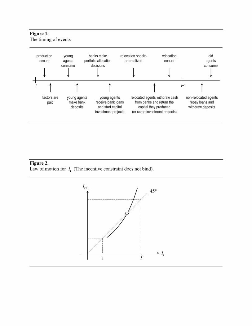
For equilibria where the nominal interest rate is not necessarily constant, equation (20) gives the equilibrium law of motion for It. The following lemma states some properties of this law of motion.

Lemma 2. Along the equilibrium law of motion given by (20) we have

0)1()1()()(1

)()(1

1 1

11

111

1>

σππ−α−⋅

γη−γη⋅

ρ−=

ρ

++

+++

+ RIA

IIII

dIdI

II t

tt

tt

t

t

t

t .

Moreover, at a steady state, 11 >+ tt dIdI .

18 If ρ>1 [γ′(I)>0] holds, then higher nominal interest rates lead banks to expand their holdings of cash reserves, and reduce their investments in capital accumulation. As a result, higher nominal rates of interest can be associated with lower rates of real growth.

18

Lemma 2 is proved in Appendix B. The lemma establishes that the equilibrium law of motion for It has the configuration depicted in Figure 2. It follows that the unique balanced growth path equilibrium is unstable. Thus, the only equilibria with positive and non-constant nominal rates of interest either have It>1 for only a finite number of periods, or else have

IIt ˆ≤ for only a finite number of periods. Since neither types of dynamical equilibria have particular interest in this context, we henceforth confine our attention to equilibria displaying constant nominal rates of interest and balanced growth.19

C. Equilibria with Binding Incentive Constraints ( IIt ˆ> )

Suppose that )ˆ(Iσ>σ holds. Then any equilibria of interest have the property that the incentive constraint (9) binds in the problem solved by banks. As a result, )(~)(ˆ II γ=γ and

)(~)(ˆ II η=η both obtain. Consequently, equation (19) reduces to

(23) σ−σ+⋅

γγ−⋅

σα−=

ηγ ++

1)(~

)(~1)1()(~)(~

1

11t

t

t

ttI

II

RA

II.

Moreover, it is easy to verify that ( ) rRIII ttt π=γγ− )(~)(~1 holds. Thus equation (23) has only trivial associated dynamics, so that there is a unique equilibrium characterized by a constant value of I. This equilibrium has the property that the economy follows a balanced growth path, which we now describe. When the nominal rate of interest is constant, and when the incentive constraint binds, equation (19) reduces to

(24) ( )IR

AII

II σ≡

−

πα−⋅

ηγ−ηγ=σ ~1)1(

)(~)(~1)(~)(~

.

It is easy to show that 0)(~ >σ′ I . Therefore, as previously, we regard equation (24) as defining the gross rate of money creation that is required in order to support any nominal rate of interest

II ˆ> as a balanced growth path equilibrium. The following lemma states an important property of the function σ~ .

Lemma 3. 1)(~)(~ ≤σσ′ III holds, and the inequality is strict if θ>0.

19 If ρ>1 [γ′(I)>0] holds, then the equilibrium law of motion described by (20) is negatively sloped. The unique balanced growth path equilibrium may be either asymptotically stable or unstable. Thus there may be many dynamical equilibrium paths consistent with perpetually positive and bounded nominal rates of interest. In addition, all such equilibria — other than the one with a constant nominal interest rate — will display oscillation, so that indeterminacy of equilibrium and endogenous volatility will emerge. It is also possible that equilibria displaying two-period cycles will exist, so that endogenously arising volatility need not vanish asymptotically.

19

The proof of Lemma 3 appears in Appendix C. The lemma has strong implications for how higher nominal rates of interest (higher rates of money growth) affect the economy’s real growth rate when the incentive constraint is binding. We now explore these implications. Equations (18) and (24) imply that, when II ˆ> holds, the equilibrium rate of growth is given by

( )I

RIIIIIII

IIAk

k

t

t )(~)(~

)(~)(~)(~)(~)(~1)(~)(~1)1(1 σ≡µ≡σηγ+ηγ−

ηγ−α−=+ .

It then follows that 01)(~)(~)(~)(~ ≤−σσ′=µµ′ IIIIII , and that the inequality is strict if θ>0. We therefore have the following result.

Proposition 2. When II ˆ> , the equilibrium rate of growth is a decreasing function of the nominal rate of interest (the rate of money growth). This function is strictly decreasing if agents do not save all of their young period income.

Intuitively, increases in the nominal rate of interest (the rate of inflation) make the incentive problem in credit markets more severe, and therefore such increases force banks to ration credit more heavily. Hence, above the threshold I (i. e. once )ˆ(~ Iσ>σ ), increases in the nominal rate of interest (the rate of money growth) cause reductions in the rate of capital investment, and reductions in the real rate of growth. The equilibrium growth rate, for all I>1, is depicted in Figure 3. Notice that this figure is consistent with a substantial body of empirical evidence suggesting that there exist threshold effects associated with the long-run rate of inflation.20 In particular, for inflation rates (or rates of money growth) below some threshold, permanent increases in the rate of inflation are associated with increases in the long-run rate of real growth. However once inflation exceeds some threshold level, further increases in it actually cause growth to decline. Our analysis offers one explanation as to why this might be the case.

D. Equilibria with Zero Nominal Interest Rates ( 1=tI ).

We now turn our attention to equilibria where the nominal rate of interest is zero. We begin with a discussion of balanced growth paths.

20 See, for instance, Bullard and Keating (1995) or Khan and Senhadji (2000).

20

1. Balanced Growth Paths

When nominal rates of interest are zero, tttt mmppR σ== ++ 11 . Moreover, the bank balance sheet constraint (5), along with the government budget constraint (3), implies that

(25) ( )tttt mAkmkσ−σ

+ +α−η=+ 11 )1()1( ; t ≥ 0.

Finally, along a balanced growth path, Rmmkk tttt σ== ++ 11 . Using this fact in (25) allows one to obtain

(26) tt kRAm)1(1

)1)(1(1η−

σ−α−η=σ−σ ; t ≥ 0.

This set of conditions completely determines a balanced growth path equilibrium with zero nominal rates of interest. Clearly several conditions must be satisfied in order for such an equilibrium to exist. One is that, with zero nominal rates of interest, banks wish to provide complete insurance against the risk of relocation. However, it is feasible for them to do so only if tt sm π≥ holds. Using (3), (2) and (26), the savings of a young agent can be written as

( ) tttt kRAmws)1(1

)1()1()1()1( 11

η−−σ−α−η=+η=

σ−σσ

−σ .

Then it is easy to verify that tt sm π≥ is satisfied iff

( )( ) ( )1

)1(1)1()1()1( σ≡

πη−π−π−α−η≤σ

RRA .

Thus, in order for the nominal rate of interest to be zero, σ≤σ(1) must hold. Once again, choosing σ≤σ(1) is feasible only if σ(1)>0. We now have a complete characterization of balanced growth path equilibria: there exists a unique equilibrium displaying balanced growth and a positive nominal interest rate if σ(1)≤0, or if σ>σ(1)>0. Otherwise, there is a unique equilibrium displaying balanced growth with I=1. Credit rationing occurs (banks face a binding incentive constraint) iff )ˆ(Iσ>σ . Finally, we note that, along a balanced growth path displaying a zero nominal rate of interest, the maximal rate of growth is achieved by setting the rate of money creation as high as possible: that is, by setting σ=σ(1). The implied rate of real growth is then ]ˆ,1[ ),()1()1( IIIR ∈∀µ≤µ=σ .

2. Dynamical Equilibria

If It=1 for all t, then tRmm tt ∀σ=+ 1 , and equation (25) can be written as

21

(27) Rm

kR

Amk

t

t

t

tσ

η−−

σα−η= σ

−σ

+

+ )1(1)1)(1( 1

1

1 ; t ≥ 0.

The law of motion described by equation (27) is depicted in Figure 4. If σ∈[0,σ(1)] holds, then it is readily established that η(1)(1-α)A>σR. Hence the unique balanced growth path is unstable. Moreover, any candidate equilibrium paths with zero nominal interest rates other than the balanced growth path have tt sm π< after a finite number of periods, and hence are not consistent with banks providing complete insurance against the event of relocation. Thus, the only possible equilibrium with a zero nominal rate of interest is the balanced growth path derived above.

V.V.V.V. WelfareWelfareWelfareWelfare

We now wish to evaluate the optimal rate of money growth along a balanced growth path. We are particularly interested to know two things: (a) whether such a rate of money creation implies positive or zero nominal rates of interest, and (b) whether such a rate of money growth implies that credit is or is not rationed. Choosing different money growth rates affects the economy through two main channels. First, higher rates of money creation (higher nominal rates of interest) are associated with more rapid rates of real growth, at least as long as )ˆ(Iσ<σ . Second, positive nominal interest rates cause banks to perceive an opportunity cost of holding cash balances, which interferes with the provision of insurance against the risk of relocation. An optimizing government must confront this trade-off. Intuitively, this logic suggests that there is little reason for an optimizing government to choose a money growth rate below σ(1) or above )ˆ(Iσ . Both of these choices would reduce the real rate of growth without improving insurance provision. However, in order to formalize this argument, we also need to consider how different rates of money creation affect the value of transfers received by young agents. We begin by considering the government’s trade-offs when ]ˆ,1( II ∈ . We then show that the government will never want to set II ˆ> , so that in an optimum credit is never rationed. Finally, we consider the government’s optimal policy among the set of policies consistent with a zero nominal rate of interest. Having done so, it will be possible to state conditions under which the Friedman rule is and is not optimal.

22

A. Positive Nominal Interest Rates and a Non-binding Incentive Constraint

Clearly we must begin by ascribing some objective function to the government. We take the government’s objective function to be the discounted sum of the expected utilities of all current and future young generations, where the government discounts the future at the rate β<1.21 We have already shown that when II ˆ1 << holds, the (maximized) expected utility of a representative member of the generation born at t is given by the expression

( ) [ ] ρ−ρ−ρ−θ η−τ+ )(11

1 ttt Iw . Furthermore, if we define the function χ(I) by

]ˆ,1( ;)()()(

1)(1)(1

IIIII

II ∈

ηγ

σ−σ−≡χ

−,

then we also have that ttt AkIw )1)(( α−χ=τ+ and ( )( ) 0kIk tt µ= , along a balanced growth

path. Thus, the welfare of a member of generation t, as a function of the equilibrium nominal rate of interest I, is

[ ] [ ] [ ] ρ−ρ−ρ−ρ−θ α−η−µχ 1

01

1 )1()(1)()( AkIII t .

It is also easy to verify that this expression gives the welfare of a representative member of generation t when σ=σ(1) holds. We can now view the government as choosing a value for the nominal rate of interest,22 ]ˆ,1[ II ∈ , to maximize

( ) [ ] ( )( )

)()(1

)()(1)()()(10

1

11I

IIIIII

t

tt Ω≡µβ−

χη−=µχη−β∑∞

=ρ−

ρ−ρ−ρ−ρ− ,

so that Ω(I) is the government’s objective function. In order for the function Ω to be well-defined, we must have II ∀<βµ ρ− ,1)( 1 . It is easy to check that this condition is satisfied if

(a.1) [ ] 1)1)(1( 1 <α−ηβ ρ−A , as we henceforth assume. Finally, let I*=argmax Ω(I); ]ˆ,1[ II ∈ The following proposition states our results about the sub-optimality of the Friedman rule. Its proof appears in Appendix D.23

21 Thus the government does not take account of the welfare of the initial old generation. We describe below how the analysis would need to be modified if the government also considered the welfare of this generation. 22 Once the optimal nominal rate of interest is chosen, the money growth rate is given by σ(I). 23 If 1>ρ holds, then the Friedman rule is suboptimal if the inequality in equation (28) is reversed.

23

Proposition 3. (a) Suppose that σ(1)>0, and that

(28) ( ) ( )[ ]ρ−µβ−πη−µ> 1)1(1)1(1)1(R is satisfied. Then it is feasible, but not optimal, to follow the Friedman rule. The optimal choice of I satisfies I*>1. (b) A sufficient condition for the Friedman rule to be sub-optimal is that )1(µ≥R .

The first inequality in part (a) of the proposition states a condition under which welfare can be increased by raising the nominal interest rate above zero. Not surprisingly, this inequality will be satisfied whenever setting I=1 leads to a sufficiently low rate of real growth. Furthermore, note that β governs the extent to which the government is willing to trade off liquidity provision for growth. For higher values of β, condition (28) is more likely to be satisfied, meaning that if the government cares about future generations more, it is more likely to want to stimulate growth by driving the nominal rate of interest above zero. Part (b) of the proposition states that the Friedman rule cannot be optimal whenever the maximal rate of growth associated with a zero nominal rate of interest is below the real rate of interest, R. This finding reflects some well-known results about golden rule allocations in conventional overlapping generations models with production. Indeed, when such models have steady states, steady state welfare is increased by promoting capital accumulation whenever the real rate of interest exceeds the rate of growth. The same kind of reasoning clearly obtains in this context as well.24 Finally, we note that this reasoning does not depend on how risk averse agents may be. This follows from the fact that, when I=1 holds, agents receive full insurance against the risk of relocation, and therefore they are locally risk neutral. Thus the Friedman rule is not optimal, and the government should raise the nominal rate of interest, whenever the real rate of interest exceeds the real rate of growth at I=1. It remains to say more about what the optimal choice I* actually is, at least over the interval ]ˆ,1[ I . Proposition 4 gives some results on this point. Its proof appears in Appendix E.

24 How would this analysis be modified if the government also cared about the welfare of the initial old generation? The consumption, and hence the welfare of this generation is affected by the choice of I only through the effect of I on the value of initial real balances. This value is easily shown to be given by γ(I)/σ(I). Thus, if the government weights the welfare of the initial old, we can represent this by appending the constraint γ(I)/σ(I)≥V to the government’s problem, where V depends on the minimum welfare level to be offered to the initial old. If this constraint is not binding at the value I=1, it continues to be the case that the Friedman rule is not optimal.

24

Proposition 4. (a) Suppose that the conditions of Proposition 3 (a) and

(29) ( ) 22111)1(

ρ−ρ+ρ+ρ− ≥µβ

are satisfied. Then II ˆ*= . (b) Suppose that the conditions of Proposition 3 (a) hold, that

(30) ( ) 221

11)ˆ(ρ−ρ+

ρ+ρ−<µβ I ,

and that ( ) ρ−µρ−≥ 1)ˆ()2(1 I all hold. Then the optimal choice of a nominal rate of

interest satisfies )ˆ,1(* II ∈ if

(31) ( ) ( )( )( ))1(1)1(1)1()1( 11 πη−µβ−µ≤π− ρ−ρρ− rR . (c) Suppose that the conditions of Proposition 3 (a) hold, that (30) holds, and that

( ) ρ−µβρ−< 1)1()2(1 . Then the optimal value of I satisfies )ˆ,1(* II ∈ if

(32) ( ) ( ) ( ))1(1)ˆ(1)ˆ()1( 11 πη−

µβ−µ≤π−ρ−ρρ− IIrR .

Proposition 4 states conditions under which the gains in real growth that derive from driving the nominal rate of interest to I are and are not large enough to overcome the associated losses in risk sharing that occur as banks economize to a greater and greater degree on their holdings of reserves.

B. Positive Nominal Interest Rates and Credit Rationing

Intuitively, there seems to be no reason for the government to increase the nominal rate of interest above the level I . Doing so does not stimulate growth, and it interferes with the provision of liquidity (insurance) by banks. However, because of the fact that money is injected via lump-sum transfers here, the possibility exists that raising the rate of money growth above

)ˆ(Iσ increases the value of the government’s objective function. This could occur if the value of the transfers received by young agents was enough to more than outweigh the other two considerations. We now demonstrate that this is not the case, and that — in fact — the optimal nominal rate of interest never exceeds I . When the incentive constraint (9) is binding in banks’ problems, we have already shown that the expected utility of a young agent born at t is ( ) ( ) ρ−ρ−

ρ−θ η−τ+ )(~11

1 Iw tt . We have also demonstrated that ttt AkIw )1)((~ α−χ=τ+ , where

)(~)(~1

1)(~

)(~)(~)(~)(~1)(~ )1(

1

IIIIIIII A

R

γη−−=

σγη+γη−≡χ α−

π−.

25

Thus the expected utility of a young agent born at t is given by the expression

( ) [ ] ( ) ρ−ρ−ρ−ρ−θ η−µχα− )(~1)(~)(~)1(

1101 IIIAk t .

If the government discounts the utility of future generations at the rate β, then over the range II ˆ> , the government’s objective function is25

( ) [ ] ( )( )

( )II

IIIIIt

tt Ω≡µβ−

χη−=µχη−β∑∞

=ρ−

ρ−ρ−ρ−ρ− ~)(~1

)(~)(~1)(~)(~)(~10

1

11.

We now state the following result.26

Proposition 5. For all ),ˆ( rRII∈ , 0)(~ ≤Ω′ I holds. The inequality is strict if θ>0.

The proof of Proposition 5 appears in Appendix F. The proposition asserts that young agents do not benefit sufficiently from higher lump-sum transfers to overturn the fact that increasing the nominal rate of interest above I interferes with both real growth, and the provision of liquidity by banks.

C. Zero Nominal Rates of Interest

It remains to consider the possibility that it is optimal for the government to set σ<σ(1). Intuitively one would expect that this choice cannot be optimal. Setting σ=σ(1) allows banks to provide complete insurance against the risk of relocation, and it maximizes the rate of real growth that is attainable with a zero nominal rate of interest. However, again the fact that money is injected via lump-sum transfers to young agents means that the consequences of these transfers must be considered in evaluating the government’s objective function. We have already demonstrated that, when nominal rates of interest are zero, the expected utility of a young agent born at t equals ( ) ( )[ ]ρρρ−ρ−ρ−

ρ−θ θ+τ+ 111

1 1 Rw tt . In addition, equation (33) implies that ( ) ttt kGw σ=τ+ , where

)1()1()1()1()(

η−σ−σ−σ−α−σ≡σ RAG .

We now state the following result. Its proof is given in Appendix G.

25 Assumption (a.1) continues to imply that the government’s objective function is well-defined for all

]/,ˆ( rRII∈ . 26 If 1>ρ holds, then it is possible that ( ) 0~ >Ω′ I holds for some II ˆ> satisfying (8). Whether this condition holds or not depends on the magnitude of β. Thus it need not be the case that the optimal choice of the nominal rate of interest is less than or equal to I .

26

Lemma 4. Suppose that )1(µ≥R . Then 0)( ≥σ′G , for all σ≤σ(1).

Lemma 4 states a simple condition under which, in the interval (0, σ(1)], the value of a young agent’s lump-sum transfer is always increased by increasing σ. Since, in this interval, increasing the rate of money growth also increases the rate of real growth, and since it does not interfere with insurance provision, it is therefore not optimal to set σ<σ(1) if the real rate of interest is greater than or equal to the maximal rate of real growth consistent with a zero nominal rate of interest. This result, together with Proposition 3, then implies that the Friedman rule is sub-optimal. Or, in other words, )1(µ≥R is a sufficient (although far from a necessary) condition for it to be desirable to have positive nominal rates of interest in this economy.

VI.VI.VI.VI. ConclusionsConclusionsConclusionsConclusions

A large literature states conditions under which it is optimal for a monetary authority to drive the nominal rate of interest to zero. And, indeed, doing so equates the social cost of creating outside money with agents’ perceptions of the opportunity cost of holding it. Nonetheless, experience suggests that having nominal rates of interest at or near zero need not lead to desirable outcomes. In fact, the closest practical approximations to the Friedman rule have been observed in places like the U.S. during the Great Depression, or in Japan recently. And, the result has invariably been a severe and long-lasting recession. This paper has pursued the notion that low nominal rates of interest can have very negative implications for real growth. In particular, when nominal rates of interest are (nearly) zero, money is a very good asset. As a result, banks have limited incentives to lend. The consequence is low rates of capital investment, and low rates of real growth. And, indeed, in situations like the Great Depression — or like that in Japan today — not only have real rates of growth been very low, but so have levels of bank lending to the private sector and rates of capital investment. When the maximal rate of real growth consistent with a zero nominal rate of interest is less than or equal to the real rate of interest, it will be desirable for the government to raise the rate of money creation, and the nominal rate of interest, in order to promote real growth.27 And, this is true essentially independently of the rate at which the government discounts the utility of future generations. 27 Of course this is true if the reserve-deposit ratio of banks is a decreasing function of the opportunity cost of holding reserves.

27

Of course there is a limit on the extent to which money creation can be used to promote growth. Considerable empirical evidence suggests that higher long-run rates of money creation can promote long-run real growth, over some range. But, this same evidence suggests that, once the rate of money creation exceeds some threshold level, further increases in the money growth rate (the rate of inflation) are — in fact — detrimental to long-run real performance. Our analysis is consistent with this finding as well. And, we have stated conditions under which a benevolent government will and will not want to push the rate of money creation to its growth maximizing level. Naturally our analysis has abstracted from a number of issues. One is the possibility that the government has revenue needs. Introducing a sequence of government expenditures would allow us to consider whether or not the government’s incentives to print money would be substantially altered by the possibility of using inflationary finance. The optimal use of such finance here would probably differ significantly from that in the existing literature on the Friedman rule (see footnote 4). And, it would raise the possibility that the government would want to regulate banks as part of an optimal tax scheme in order to enhance the inflation tax base.28 Another obvious extension of the analysis would be to allow the government to issue (potentially) interest bearing bonds as well as money. If seigniorage income can be used to pay interest on government bonds, the nature of the relationship between inflation and real rates of growth can be substantially different from the one demonstrated above.29 It would be interesting to see how these modifications of the analysis would affect the optimality of the Friedman rule.

28 See, for instance, Bencivenga and Smith (1992), Bhattacharya, et. al. (1997), or Espinosa and Yip (2000). 29 This point is discussed by Schreft and Smith (1997).

28

ReferencesReferencesReferencesReferences

Azariadis, Costas and Smith, Bruce D. (1996). Private information, money, and growth: Indeterminacy, fluctuations, and the Mundell-Tobin effect. Journal of Economic Growth, 1(3), pp. 309-332.

Beck, Thorsten, Levine, Ross and Loayza, Norman (2000). Financial intermediation and growth: Causes and causality. Journal of Monetary Economics, 46(1), pp. 31-77.

Bencivenga, Valerie R. and Smith, Bruce D. (1992). Deficits, inflation, and the banking system in developing countries: The optimal degree of financial repression. Oxford Economic Papers, 44(4), pp. 767-790.

Bhattacharya, Joydeep, Guzman, Mark, Huybens, Elisabeth and Smith, Bruce D. (1997). Monetary, fiscal and reserve requirement policy in a simple monetary growth model. International Economic Review, 38 (2), pp. 321-350.

Boyd, John H., Choi, Sangmok and Smith, Bruce D. (1996). Inflation, financial markets and capital formation. Federal Reserve Bank of Saint Louis Review, 78(3), pp. 9-35.

Boyd, John H. and Smith, Bruce D. (1998). Capital market imperfections in a monetary growth model. Economic Theory, 11(2), pp. 241-273.

Bruno, Michael and Easterly, William (1998). Inflation crises and long-run growth. Journal of Monetary Economics, 41(1), pp. 3-26.

Bryant, John and Wallace, Neil (1984). A price discrimination analysis of monetary policy. Review of Economic Studies, 51(2), pp. 279-88.

Bullard, James and Keating, John W. (1995). The long-run relationship between inflation and output in postwar economies. Journal of Monetary Economics, 36(3), pp. 477-496.

Champ, Bruce, Smith, Bruce D. and Williamson, Stephen D. (1996). Currency elasticity and banking panics: Theory and evidence. Canadian Journal of Economics, 29(4), pp. 828-864.

Chari, V.V, Christiano, Lawrence J. and Kehoe, Patrick J. (1996). Optimality of the Friedman rule in economies with distorting taxes. Journal of Monetary Economics, 37(2), pp. 203-223.

Correia, Isabel and Teles, Pedro (1996). Is the Friedman rule optimal when money is an intermediate good? Journal of Monetary Economics, 38(2), pp. 223-244.

29

Diamond, Douglas W. and Dybvig, Philip H. (1983). Bank runs, deposit insurance, and liquidity. Journal of Political Economy, 91(3), pp. 401- 419.

Espinosa, Marco A. and Yip, Chong K. (forthcoming). Government financing in an endogenous growth model with financial market restrictions. Economic Theory.

Greenwood, Jeremy and Smith, Bruce D. (1997). Financial markets in development and the development of financial markets. Journal of Economic Dynamics and Control 21(1), pp.145-181.

Guidotti, Pablo and Vegh, Carlos (1993). The optimal inflation tax when money reduces transaction costs. Journal of Monetary Economics, 31(2), pp. 189-205.

Hornstein, Andreas and Krusell, Per (1993). Money and insurance in a turnpike environment. Economic Theory, 3(1), pp. 19-34.

Ireland, Peter (1996). The role of countercyclical monetary policy. Journal of Political Economy, 104(4), pp.704-723.

Kahn, Moshin and Senhadji, Abdelhak (2000). Threshold effects in the relationship between inflation and growth. Manuscript.

Keynes, John Maynard (1936). The general theory of employment, interest, and money. New York: Harcourt, Brace.

Kimbrough, Kent P. (1986). The optimum quantity of money rule in the theory of public finance. Journal of Monetary Economics, 18(3), pp. 277-284.

King, Robert G. and Levine, Ross (1993a). Finance and growth: Schumpeter might be right. Quarterly Journal of Economics, 108(3), pp. 717-737.

King, Robert G. and Levine, Ross (1993b). Finance, entrepreneurship and growth: Theory and evidence. Journal of Monetary Economics, 32(3), pp. 513-542.

Levine, David (1991). Asset trading mechanisms and expansionary policy. Journal of Economic Theory, 54(1), pp. 148-164.

Mitsui, Toshihide and Watanabe, Shinichi (1989). Monetary growth in a turnpike environment. Journal of Monetary Economics, 24(1), pp. 123-37.

Mulligan, Casey and Sala-i-Martin, Xavier (1997). The optimum quantity of money: Theory and evidence. Journal of Money, Credit and Banking, 29(4), pp. 687-715.

Phelps, Edmunds S. (1973). Inflation in the theory of public finance. Swedish Journal of Economics, 75(1), pp. 67-82.

Romer, Paul M. (1986). Increasing returns and long-run growth. Journal of Political Economy, 94(5), pp. 1002-37.

30

Schreft, Stacey and Smith, Bruce D. (1997). Money, banking and capital formation. Journal of Economic Theory, 73(1), pp. 157-182.

Schreft, Stacey and Smith, Bruce D. (1998). The effects of open market operations in a model of intermediation and growth. Review of Economic Studies, 65(3), pp. 519-550.

Shell, Karl (1966). Toward a theory of inventive activity and capital accumulation. American Economic Review, 56(2), pp. 62-68.

Smith, Bruce D. (1991). Interest on reserves and sunspot equilibria: Friedman’s proposal reconsidered. Review of Economic Studies, 58(1), pp. 93-105.

Townsend, Robert M. (1987). Economic organization with limited communication. American Economic Review, 77(5), pp. 954-971.

Wallace, Neil (2000). Another example where lump-sum money creation is beneficial. Manuscript.

Williamson, Stephen D. (1996). Sequential markets and the sub-optimality of the Friedman rule. Journal of Monetary Economics, 37(3), pp. 549-572.

Woodford, Michael (1994). Monetary policy and price level determinacy in a cash-in-advance economy. Economic Theory, 4(3), pp. 345-380.

31

AppeAppeAppeAppendix ndix ndix ndix

A. Proof of Lemma 1.

Part (a) of the lemma follows immediately from the definition of σ(I) in equation (21), and the fact that γ(1)=π. Parts (b) and (c) follow from the fact that

(A.1) ( )( ) RIA

IAII

IIIII

π−π−α−π−α−ρ+

ψ−ψψ′=

σσ′

ρ

ρ−

1

11

)1()1()1()1(

)(11

)()( ,

where ψ(I)≡γ(I)η(I), and where

(A.2) ( ) ( )( )

=ξθ+

ξθγ−γ−−=γγ′+

ηη′=

ψψ′

ρ−ρ

ρ−ρ

ρρ−

ρρ−

11

1111

)(1)()()(1

)()(

)()(

)()(

IIII

III

III

III

( )( )

( ))(1)(1

)(1)(1 111

111 I

III ψ−−=

ξθ+ξθ−γ−− ρ

ρ−ρ−ρ

ρ−ρ

ρρ− .

Substituting (A.2) into (A.1) and rearranging terms yields

(A.3) 1)1()1(

1)()(

1

1>

π−π−α−πρ+=

σσ′

ρ

−

RIAR

III ,

completing the proof.

B. Proof of Lemma 2

Let ψ(I)≡γ(I)η(I). Then, differentiating equation (26) yields

(A.4) ( )( ) ( )[ ]σ−σ+πσα−π−

πσα−π−ρ=

ψψ′− ρ

ρ−+

++

++

1)1)(1()1)(1(

)()(

1

111

11

11

t

t

t

t

t

t

t

ttIRA

IRAdI

dIII

III .

Substituting (A.3) and (20) into (A.4) one obtains the expression in the lemma. Moreover, along a balanced growth path,

( ) )(1)1)(1()( 11 IIRAI t ψ−=πσα−π−ψ σ−σρ

is satisfied. Thus, when It is constant,

1)(1

)(1)1(

111 >

ψ−ψ−

ρ−= σ−σ

−+I

IdI

dIt

t

holds, as claimed.

32

C. Proof of Lemma 3.

From the definition of σ~ we have

(A.5) ( )( ) )(~1

1)(~)(~

~~

IIII

III

ψ−ψψ′=

σσ′ ,

where, as before, we define )(~)(~)(~ III ηγ=ψ . In addition, it is easy to show that

(A.6) ( ))(~)(~)(~)(~1)(~)(~

1 IIIIIII ηγ−γρ−ψ−=

ψψ′ − .

The claim then follows from (A.5) and (A.6), along with the observation that 1)(~ <η I holds if θ>0.

D. Proof of Proposition 3.

In order to prove Proposition 3, it will be useful to begin with the following lemma. Lemma A.1. The function χ(I) has the representation

( ) ( ))(1)()1()(

IIAII

γ−ηα−µ=χ .

Proof of Lemma A.1. The definitions of the functions χ(I) and σ(I) imply that

( )( ) ( )( )=π−α−ηγ−

π−π−α−=ηγ−

=χ ρ

ρ

σ−σ 1

1

1 11)()(1)1()1(

)()(11)(

IAIIRIA

III

( ) ( ))(1)()1(

)()()(1

)(11 IIA

IIIIA

IIγ−ηα−

µ=γηα−

µρ

ππ−

,

as claimed. To continue with the proof of Proposition 3, define the function H(I) by

(A.7) ( ) ( )( ) 11)(1−ρ−µβ−≡ IIH .

Then equation (A.7) and Lemma A.1 imply that the government’s objective function takes the form

(A.8) ( ) ( )ρ−

ρ−

γ−η

µη−=Ω1

)(1)()()(1)()(

IIIIIHI .

It then follows from (A.8) that

(A.9) ( )

γ−

γ′−µµ′−

ηη′ρ−−

η−η′ρ+

′=

ΩΩ′

)(1)(

)()(

)()(1

)(1)(

)()(

)()(

III

III

III

III

IHIHI

III .

33

Moreover, we observe that

(A.10) )()(1

)( 1 II

II γ−=γ−γ′

ρρ− ,

(A.11) ( )( ) )(

)()(1

)()1()()(

1

1

III

II

IHIHI

µµ′

µβ−µβρ−=

′ρ−

ρ−

(A.12) ( ))(1)()(1

)( 1 III

II η−γ−=η−η′

ρρ− ,

and

(A.13) ( ))()(1)()()(

)()(

IIIIIIR

III

ηγ−µρηγ=

µµ′ .

Substituting equations (A.10)–(A.13) into (A.9) and rearranging terms yields

( ) ( )( )

−

µβ−µηγ−ηγ=

ΩΩ′

ρ−ρρ− 1

)(1)()()(1)()(

)()(

11

IIIIIRII

III .

It follows that Ω′(1)>0 holds iff

(A.14) ( ) ( )( )ρ−µβ−πη−µ> 1)1(1)1(1)1(R , where (A.14) follows from the fact that γ(1)=π. This establishes part (a) of the proposition. Part (b) is then immediate, since ( )( )ρ−βµ−πη−> 1)1(1)1(11 .

E. Proof of Proposition 4.

Define the function Q(I) by

(A.15) ( ))(1)()()(

IIIIRHIQψ−µ

≡ ,

where, as before, ψ(I)≡γ(I)η(I), and where the function H(I) is defined in (A.7). Then Appendix D establishes that Ω′(I)≥0 holds iff Q(I)≥1. And, if the conditions of Proposition 3 (a) hold, Ω′(1)>0 [Q(1)>1] is satisfied. Differentiating (A.15) yields

(A.16) )(1

1)()(

)()(1

)()(

)()(

IIII

III

IHIHI

IQIQI

ψ−ψψ′+

µµ′−−

′=

′.

Substituting (A.2), (A.11) and (A.13) into (A.16) and rearranging terms, we obtain

( )( )( )ρ−

ρ−

µβ−ρρ+−µρ−ρ+β=

′1

12

)(1)1()()21(

)()(

II

IQIQI .

Thus, if

(A.17) ( ) 22111)(

ρ−ρ+ρ+ρ− ≥µβ I

34

is satisfied for all ]ˆ,1( II∈ , and if the conditions of Proposition 3 (a) hold, Q(I)>1 is satisfied for all ]ˆ,1[ II∈ . Moreover, (A.17) is satisfied for all I if (29) holds. It follows that II ˆ*= . This establishes part (a) of the proposition. For parts (b) and (c), satisfaction of (30) is required in order for )1()ˆ( QIQ < to hold. Moreover, 1)ˆ( <IQ ]0)ˆ([ <Ω′ I is satisfied iff

( ) ( ) ( )ρρ−ρ−π−≡>

µβ−ψ−µ rR

IRIII )1(ˆ)ˆ(1)ˆ(1)ˆ( 11 .

In addition, since ψ(I) is a decreasing function, it follows that )1(1)1(1)ˆ(1 πη−=ψ−>ψ− I . Finally, it is straightforward to show that the term ( )( )ρ−µβ−µ 1)(1)( II is increasing in I iff

(A.18) ( ) ρ−µβρ−≥ 1)()2(1 I . Thus if

(A.19) ( ) 22111)(

ρ−ρ+ρ+ρ− >µβ I

and (A.18) are satisfied for all ]ˆ,1( II∈ , and if the conditions of Proposition 3 (a) hold, then equation (31) is sufficient for 1)ˆ( <IQ ]0)ˆ([ <Ω′ I to hold. Moreover, (A.18) and (A.19) are satisfied for all I if ( ) ρ−

µβρ−≥ 1)ˆ()2(1 I and (30) hold. Hence II ˆ*< obtains. Similarly, if (A.19) holds but (A.18) is violated for all ]ˆ,1( II∈ , then equation (32) is sufficient for

1)ˆ( <IQ ]0)ˆ([ <Ω′ I to be satisfied. Since ( ) ρ−µβρ−< 1)1()2(1 implies that ( ) ρ−µβρ−< 1)()2(1 I for all I, we again have II ˆ*< . This establishes the proposition.

F. Proof of Proposition 5.

Straightforward differentiation yields

(A.20) ( )( ) )(~1

)(~)1(

)(~1)(~

)(~)(~

)(~1)(~)1(

)(~)(~

1

1

III

III

III

II

III

ψ−ψ′ρ−+

η−η′ρ+

µµ′

µβ−µβρ−=

ΩΩ′

ρ−

ρ−,

where )(~)(~)(~ III ηγ=ψ . Substituting (14) and (A.6) into (A.20) gives

( )( )

ψ−ψ−γρ−ψρ−+ψρ−−

µµ′

µβ−µβρ−=

ΩΩ′ −

ρ−

ρ−

)(~1)(~)(~

1)(~)1()(~)1()(~)(~

)(~1)(~)1(

)(~)(~

11

1

IIIII

III

II

III

Since 0)(~ ≤µ′ I , it follows that, for all II ˆ> , 0)(~ ≤Ω′ I . Moreover, the inequality is strict if θ>0, so that )(~)(~)(~)(~ IIII γ<ηγ≡ψ .

G. Proof of Lemma 4.

Straightforward differentiation implies that

RA

RGG

)1()1()1(1)1(

)()(

1 −σ−α−−

η−η=

σσ′

σ−σ .

35

Note, then, that G′(σ)>0 necessarily holds if (σ–1)R > (1–α)A. And, if (σ–1)R < (1–α)A holds, then G′(σ)>0 is satisfied iff

(A.21) ( ))1(1)1)(1( 12 η−σ≥α−η σ−σRA .

Since σ≤σ(1), note that a sufficient condition for (A.21) to obtain, and hence for G′(σ)>0 to hold, is that

(A.22) 2)1()1)(1( σ≥α−η RA . Now, since IRII )()( σ≡µ , it follows that RR 22 )1()1( µ≡σ . Moreover, it is easy to verify that AAII )1)(1()1)(()( α−η≤α−η≤µ , for all I. Then (A.22) is satisfied if ( ) )1()1()1)(1( µµ≥α−η RA . But this necessarily holds if R≥µ(1).

Figure 1. The timing of events

t t+1

banks make portfolio allocation

decisions

young agents make bank

deposits

young agents receive bank loans

and start capital investment projects

production occurs

relocation shocks are realized

relocated agents withdraw cash from banks and return the

capital they produced (or scrap investment projects)

relocation occurs

non-relocated agents repay loans and

withdraw deposits

old agents

consume

young agents

consume

factors are paid

Figure 2. Law of motion for It (The incentive constraint does not bind).

It

It+1 45°

1 I

Figure 3. Equilibrium growth rate.

I 1 I R/r

µ(I) )(~ Iµ

)(ˆ Iµ

Figure 4. Law of motion for kt/mt. (Zero nominal rates of interest)

45°

t

tmk

1

1

+

+

t

tmk