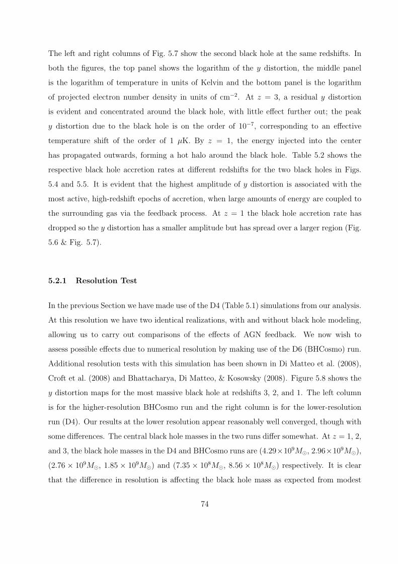
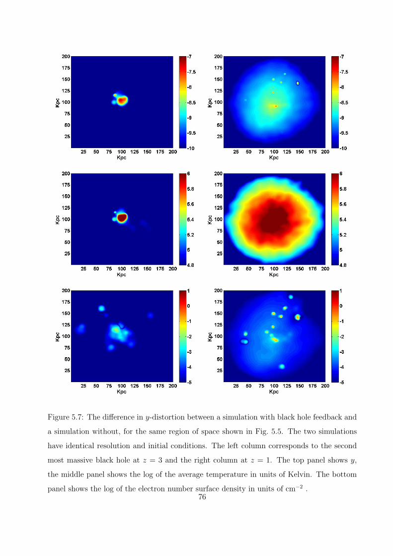
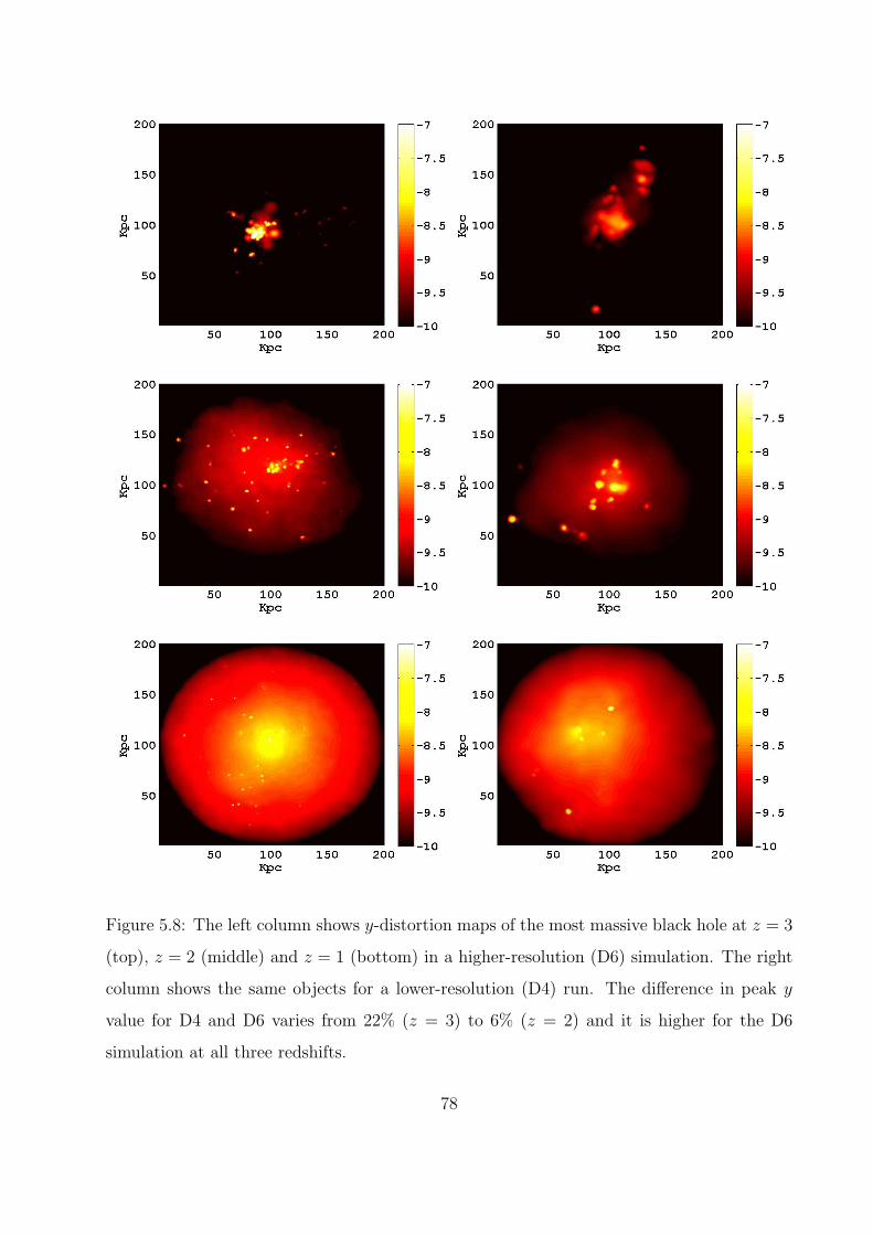
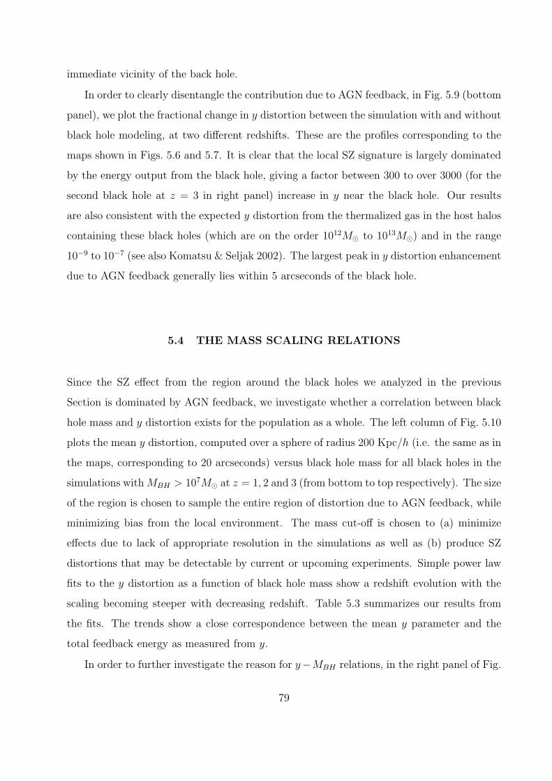
THE SUNYAEV-ZELDOVICH EFFECT AS A PROBE OF BLACK HOLE FEEDBACK by Suchetana Chatterjee Bachelor of Science, Presidency College (Calcutta University), 2001 Master of Science, Indian Institute of Technology, Kanpur, 2003 Submitted to the Graduate Faculty of the Department of Physics and Astronomy in partial fulfillment of the requirements for the degree of Doctor of Philosophy University of Pittsburgh 2009
Transcript
THE SUNYAEV-ZELDOVICH EFFECT AS A
PROBE OF BLACK HOLE FEEDBACK
by
Suchetana Chatterjee
Bachelor of Science, Presidency College (Calcutta University), 2001
Master of Science, Indian Institute of Technology, Kanpur, 2003
Submitted to the Graduate Faculty of
the Department of Physics and Astronomy in partial fulfillment
of the requirements for the degree of
Doctor of Philosophy
University of Pittsburgh
2009
UNIVERSITY OF PITTSBURGH
DEPARTMENT OF PHYSICS AND ASTRONOMY
This dissertation was presented
by
Suchetana Chatterjee
It was defended on
August 3, 2009
and approved by
Arthur Kosowsky, Associate Professor
David Turnshek, Professor and Department Chair
John Hillier, Professor
Chandralekha Singh, Associate Professor
Grant Wilson, Assistant Professor
Dissertation Director: Arthur Kosowsky, Associate Professor
where c is the speed of light and dσ/dΩ is the scattering cross-section. The scattering term is
proportional to the scattering cross-section (which will be Thompson scattering cross-section
if the energy of the electrons is much lower than the rest mass of the electrons), and the
interaction term in the Lagrangian. The Compton scattering process can be written in terms
of a two way process from the conservation of energy and momentum as
P + ω P1 + ω1. (2.18)
23
In the forward scattering, there is a creation of states P1 and ω1, and annihilation of states P
and ω. I can write the forward scattering term as (a†|n(ω1)〉)(a|n(ω)〉)(b†|fe(P1)〉)(b|fe(P )〉),where a, a†, b, and b† are the bosonic and fermionic annihilation and creation operators
respectively in the Fock representation. The backward scattering term will be creation
of states P and ω and annihilation of states P1 and ω1 and would be proportional to
(a†|n(ω)〉)(a|n(ω1)〉)(b†|fe(P )〉)(b|fe(P1)〉). Using the eigenvalues for the operators, I get the
entire matrix element for the forward scattering term as (1 + n(ω1))(1− fe(P1))fe(P )n(ω),
and the backward scattering process as (1 + n(ω))(1− fe(P ))fe(P1)n(ω1). For a dilute non-
degenerate distribution of electrons, 1 − fe ≈ 1. With this approximation I can write the
change in the photon phase-space density in the form given in Eq. 2.17.
I consider a small fractional energy transfer between the photons and the electrons. This
enables me to expand fe(P1) and n(ω1) in terms of fe(P ) and n(ω).
n(ω1) = n(ω) + (ω1 − ω)∂n(ω)
∂ω+ 1/2(ω1 − ω)2∂
2n(ω)
∂ω2, (2.19)
fe(E1) = fe(E) + (E1 − E)∂fe(E)
∂E+ 1/2(E1 − E)2∂
2fe(E)
∂E2, (2.20)
where E1 = P 21 /2me, E = P 2/2me, and me is the mass of the electron. I define the following
variables,
∆ =h(ω1 − ω)
KBTe, (2.21)
x =hω
KBTe. (2.22)
KB is Boltzmann constant and Te is the temperature of the electrons. Using Eq. 2.19, 2.21,
and 2.22 I get
n(ω1) = n(ω) + ∆n′+
∆2
2n′′, (2.23)
where the derivatives are with respect to x. For a Maxwellian distribution of electrons we
can write ∂fe/∂E = −(1/KBTe)fe, and ∂2fe/∂E2 = (1/(KBTe)
2)fe. Using Eq. 2.20, I get
fe(E1) = fe(1 + ∆ + ∆2/2). (2.24)
24
I can now use Eq. 2.17, 2.23, and 2.24 to get
∂n
∂t= c
∫d3P
∫dσ
dΩdΩ[fe(E)(1 + ∆ +
∆2
2)
(n+ ∆n′+
∆2n′′
2)(1 + n)− fe(E)n(1 + n+ ∆n
′+
∆2n′′
2)]. (2.25)
Keeping second order terms in ∆, I get
∂n
∂t= c(n
′+ n(1 + n))
∫ ∫d3P
dσ
dΩdΩfe∆ +
c
(n′′
2+ n
′(1 + n) +
n(1 + n)
2
)∫ ∫d3P
dσ
dΩdΩfe∆
2. (2.26)
Equation 2.26 is the Fokker-Plank expansion of the Boltzmann equation in orders of the
energy transfer. The term involving ∆2 is the random walk term and the term involving ∆
is called the secular term.
To evaluate the integral, I need to know the energy transfer ∆. I evaluate ∆ by applying
the energy momentum conservation relations. Let the initial and final 4-momentum of the
photon be Pγ = (1, n)hω/c and Pγ1 = (1, n1)hω1/c, and the initial and final momentum of
the electron be Pe = (E/c, P ) and Pe1 = (E1/c, P1), where n and n1 are the unit direction
vectors before and after the scattering event. Now applying the conservation of 4-momentum
I get
|Pe1|2 = |Pe + Pγ − Pγ1|2. (2.27)
This gives
E21
c2− P 2
1 =E2
c2− P 2 + 2hω
E
c2− 2P.nhω
c− 2h2ω1ω
c2(1− n.n1)− 2hω1
E
c2+
2P.n1hω
c. (2.28)
Here I have explicitly used the fact that the 4-momentum of the photon is zero since it does
not have a rest mass. Now using Eq. 2.21, I can write
ω1 =KBTe∆
h+ ω. (2.29)
Using Eq. 2.29, I can write Eq. 2.28 as
Ehω
c−hωP.n =
h2ω
c(1−n.n1)
(ω +
KBTe∆
h
)+Eh
c
(ω +
KBTe∆
h
)−hP.n1
(ω +
∆KBTeh
).
(2.30)
25
Using the expression for x = hω/(KBTe), I have
∆ =xp(n1 − n)− x2KBTe
c(1− n.n1)
E/c− P.n1 + xKBTe(1− n, n1). (2.31)
For non-relativistic electrons E = mec2, and thus I can write
∆ =x.p(n1 − n)
mec+O(KBTe/mec
2). (2.32)
I will now evaluate the integral involving the term ∆2 in Eq. 2.26. Let,
I2 =
∫d3Pfe∆
2
∫dσ
dΩdΩ. (2.33)
Let χ be the angle between P and (n1 − n) and d3P = P 2dPdΩ′. If I choose χ to be the
polar angle in the Ω′
integral and if n1 lies along the polar axis in the Ω integral, I can write
I2 as a product of three integrals (Rybicki & Lightman 1985) given as
I2 =nex
2
(mec)2(2πmeKBTe)
−3/2
∫P 4 exp
( −P 2
2meKBTe
)dP
∫ ∫cos2 χ sinχdχdφ
′
∫ ∫3σT8π
(1 + cos2 θ)(1− cos θ) sin θdθdφ, (2.34)
where dσ/dΩ = (3σT/(16π))(1+cos2 θ) (Rybicki & Lightman 1985) and σT is the Thompson
cross section. The (1 − cos θ) factor comes from the (n1 − n) term. After evaluating the
three integrals, I get
I2 =nex
2
(mec)2(2πmeKBTe)
−3/2 [(3/4)(2meKBTe)3/2meKBTeπ
1/2]
(4π/3)(2σT )
=2σTKBTenex
2
mec2. (2.35)
My next step involves evaluating the integral with the secular term in the Fokker-Planck
equation. This can be achieved in a similar way, but I will adopt a simpler method for
evaluating the integral using the photon number conservation. Since n is the photon phase
space density and x is proportional to the momentum of the photons, than from conservation
of photon number I have,
d
dt
∫nx2dx = 0 =
∫∂n
∂tx2dx. (2.36)
26
Nowd
dt
∫nx2dx = −
∫∂
∂x(x2j(x))dx, (2.37)
Eq. 2.37 implies that the change in total flux arises only from flux through the boundaries.
Here j(x) is a function of x only. This comes from the continuity equation where the x2j(x)
term is the equivalent of current density. From Eq. 2.36 and 2.37 I have
(∂n
∂t
)x2 = − ∂
∂x(x2j(x)). (2.38)
I need to find the functional form of j(x). According to Eq. 2.26, I have
∂n
∂t= C1(x)n
′′+ C2(x, n)n
′+ C3(n, x), (2.39)
where C1, C2 and C3 are the coefficients to be determined. Comparing Eq. 2.39 and 2.26, I
know that j(x) should have a term involving n′
with coefficients independent of n. So the
most general form of j(x) can be written as
j(x) = g(x)(n′+ h(n, x)), (2.40)
where h and g are two functions to be determined. The photons follow the Bose-Einstein
distribution. This gives
n =1
ex+α − 1(2.41)
∂n
∂x= −n(n+ 1), (2.42)
where α is the chemical potential. I can match the boundary condition for an equilibrium
distribution and this will give ∂n/∂t = 0. Now, ∂n/∂t = 0 will require the current density
to be a constant (Rybicki & Lightman 1985), but that can be achieved only by assuming
j(x) = 0, otherwise the current flux will blow up. Thus using Eq. 2.40, I have
n′= −h(n, x)
h(n, x) = n(n+ 1). (2.43)
Using Eq. 2.38 and 2.40 we have
∂n
∂t= −(g
′n′+ gn
′′+ h
′g + g
′h+ 2n
′g/x+ 2hg/x), (2.44)
27
where the primes are derivatives with respect to x. Comparing Eq. 2.26, 2.39, and 2.44, I
have
c
2I2 = −g(x)
g(x) = −cx2neσTKBTemec2
. (2.45)
Using Eq. 2.43 and 2.45, I get the full form of j(x) as
j(x) = −cx2neσT
(KBTemec2
)(n′+ n(n+ 1)). (2.46)
Using the form of j(x) in Eq. 2.38, I get the following equation :
∂n
∂t= (cneσT )
(KBTemec2
)1
x2
∂
∂x
(x4(n
′+ n+ n2)
). (2.47)
Equation 2.47 is known as the Kompaneets equation (Kompaneets 1957) which is the non
relativistic approximation of the Boltzmann equation with small energy transfers. I will now
do a transformation of variable which will involve in going from the electron temperature
to the temperature of radiation (Zeldovich & Sunyaev 1969). Let y = (hω)/(KBTr), where
Tr is the temperature of the radiation field. For the present case this will correspond to the
CMB temperature of 2.73 K. Changing variables from x to y gives the Kompaneets equation
as follows (Rephaeli 1995),
∂n
∂t= (cneσT )
(KBTemec2
)1
y2
TrTe
∂
∂y
(y4
(n′ TeTr
+ n+ n2
)), (2.48)
where the derivatives are taken with respect to y now.
If the temperature of the electrons is large compared to the temperature of radiation,
which is the case for cluster X-ray gas (kev electrons) with reference to the CMB (mev
photons), then the first term in Eq. 2.48 dominates, and the Kompaneets equation takes the
following form (Zeldovich & Sunyaev 1969, Rephaeli 1995)
∂n
∂t= yneσT
KBTemec
(y∂2n
∂y2+ 4
∂n
∂y
). (2.49)
In the limit of weak scattering, I can perturbatively expand the photon distribution function
in orders of y with respect to the equilibrium distribution function. To first approximation
this will enable me to write the distribution function as of purely Planckian nature with no
28
chemical potential. Using this distribution function for n given as, n = 1/(ey − 1), ∂n/∂y =
−ey/(ey − 1)2, and ∂2n/∂y2 = 2ey/(ey − 1)3 − ey/(ey − 1)2, I have Eq. 2.49 written as
∂n
∂t= neTe
KBσTmec
yey
(ey − 1)2
(y(ey + 1)
(ey − 1)− 4
). (2.50)
Now the intensity of the photon distribution is given as
I =2hν3
c2(ey − 1)= i0y
3n, (2.51)
where i0 = 2 (KBTr)3
(hc)2 . Using Eq. 2.50 and 2.51, I get the change in the intensity of the photon
distribution due to the up scattering process:
∆I =
∫i0y
3∂n
∂t
dl
c=
∫neTe
KBσTmec2
y4ey
(ey − 1)2
(y(ey + 1)
(ey − 1)− 4
)dl
= i0G(y)
∫neTe
KBσTmec2
dl = i0G(y)Y. (2.52)
The above integral is done along the line of sight of the cluster and Y is defined as the
Compton Y parameter and G(y) is the spectral distortion. The Compton Y parameter
is designated by “y” in the literature and so I will now use the notation “y” to denote
the Compton y parameter. For clarity I will denote the dimensionless parameter y by
x (as popularly done in the literature), such that x = hω/(KBTr) = hω/(KBTCMB) =
hν/(KBTCMB). So for an inverse Compton scattering of the CMB photons by non relativistic
electrons in clusters, I get a spectral distortion in the CMB given by the function G(x) such
that
G(x) =x4ex
(ex − 1)2
(x(ex + 1)
(ex − 1)− 4
), (2.53)
where x = hω/(KTCMB). The change in intensity is proportional to the product of the
spectral distortion and the y parameter which is an integrated line of sight pressure of the
cluster gas (Sunyaev & Zeldovich 1972) and is given by
y =KBσTmec2
∫neTedl, (2.54)
where ne and Te are the number density and temperature of the electron gas in the cluster,
andKB, σT , me, and c are Boltzmann constant, Thomson scattering cross section, mass of the
29
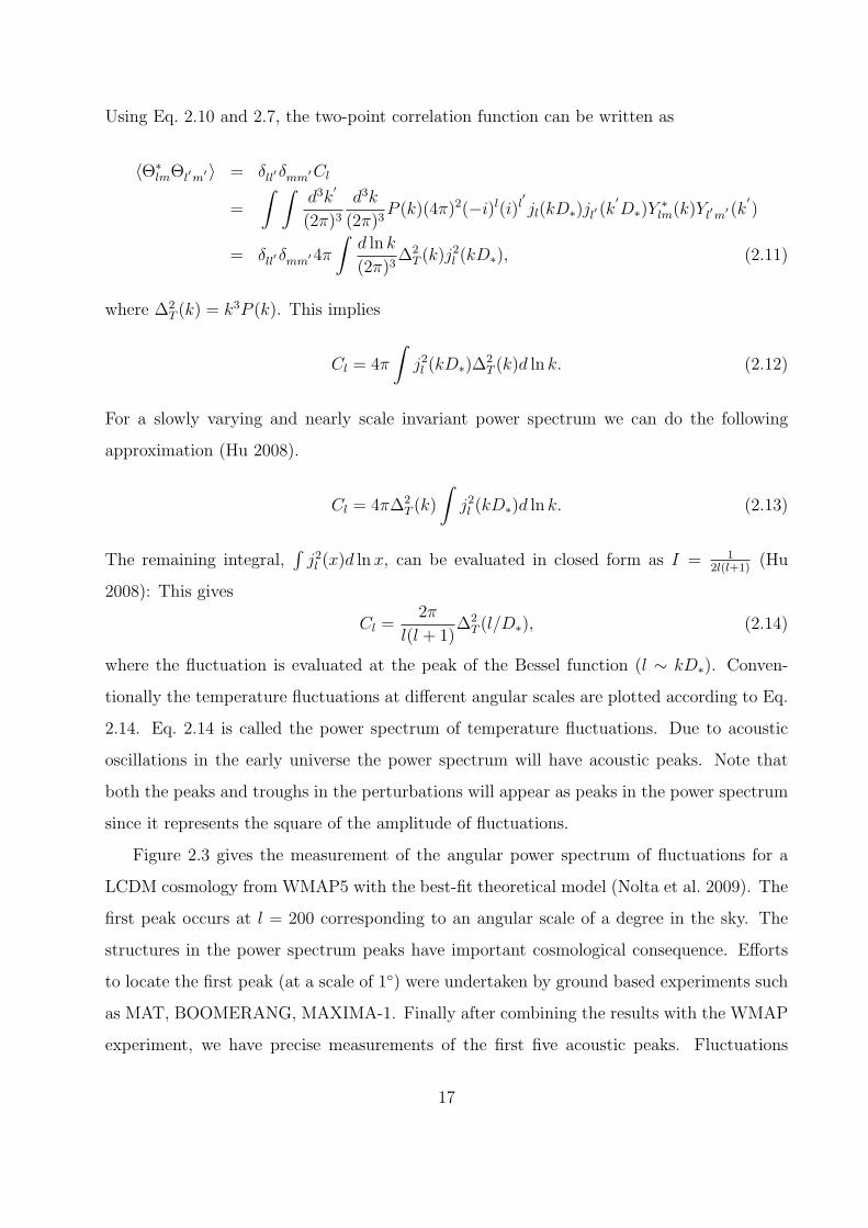
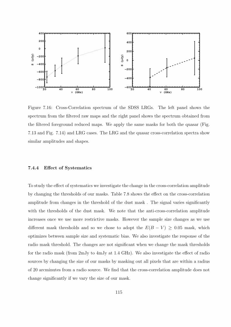
100 150 200 250 300−2
−1.5
−1
−0.5
0
0.5
1
1.5
ν (GHz)
f(
ν)
100 150 200 250 300−6
−4
−2
0
2
4
6
ν (GHz)
G(
ν)
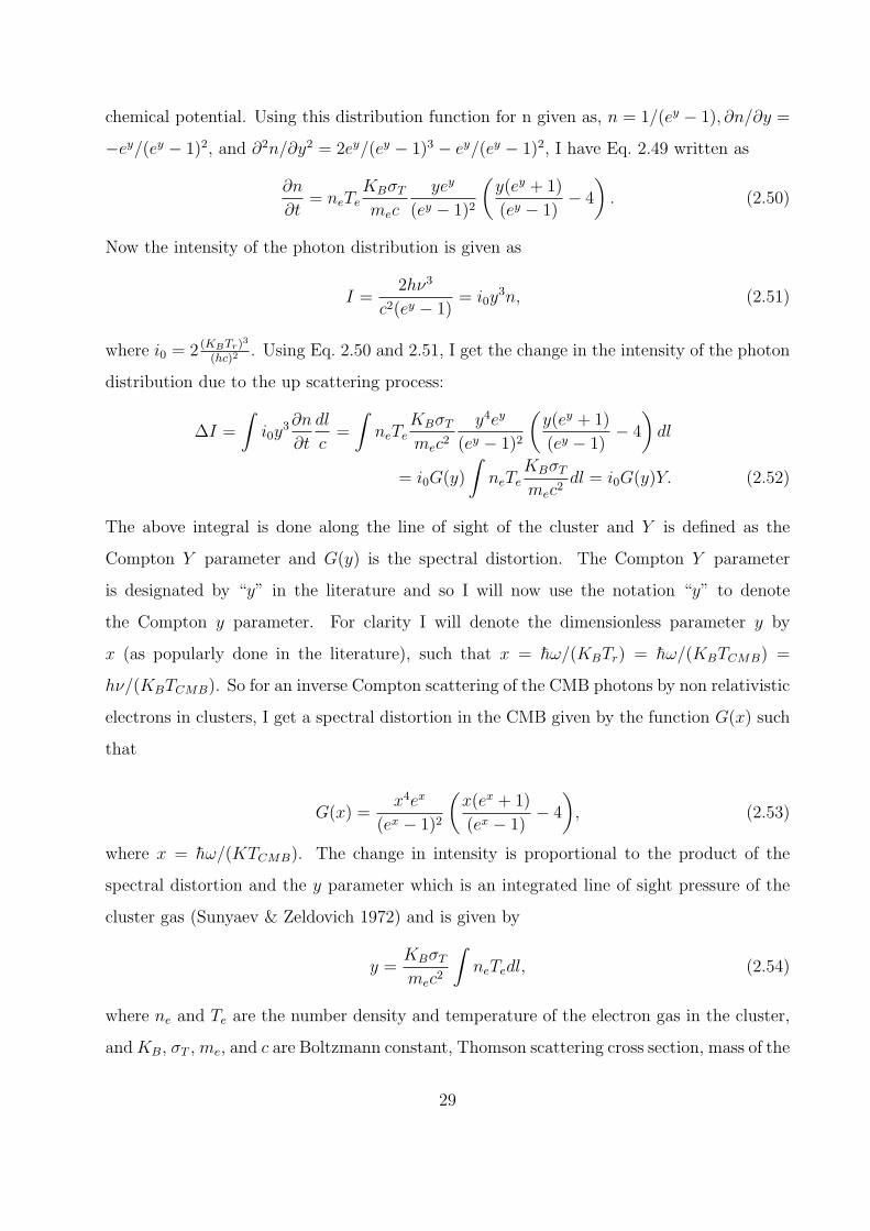
Figure 2.4: Frequency variation of the two functions f(ν)(Eq. 2.57) and G(ν) (Eq. 2.53)
where ν = KBTCMBx/h
electron, and speed of light respectively. Now the change in intensity can be characterized
as a temperature change in the CMB. I can write the following transformation between
intensity and temperature.
∆I =2hν3
c2
ex
(ex − 1)2
hν
KBT 2CMB
∆T. (2.55)
Using Eq. 2.55, 2.53, and 2.52 I get
∆T = TCMByf(x), (2.56)
where
f(x) =
(x(ex + 1)
(ex − 1)− 4
). (2.57)
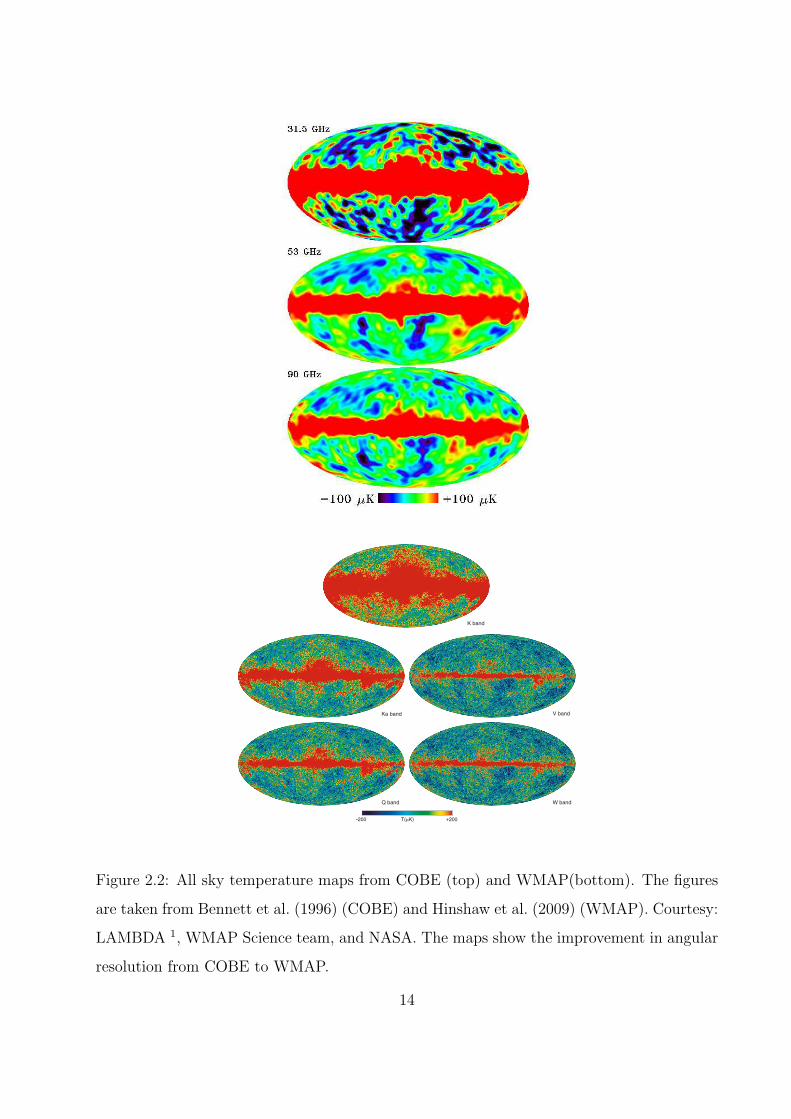
In Fig. 2.4 the functional dependence of G(x) and f(x) on frequency are shown for a fixed
CMB temperature of 2.73 K. At 220 GHz the functions become zero. This frequency is
defined as the null frequency of the SZ effect. Below the null frequency we see a decrement in
intensity and above the null frequency we see an enhancement in the intensity. This manifests
as hot and cold spots in the CMB. Note that the SZ distortion is a spectral distortion and
30
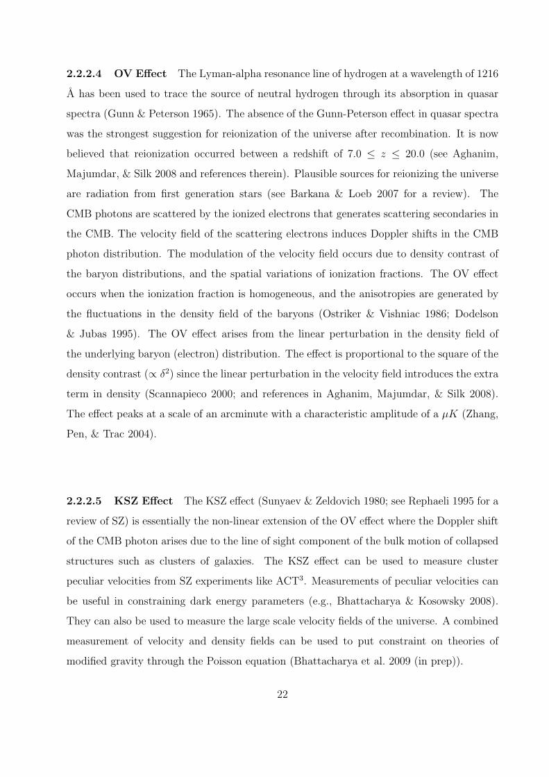
0 200 400 600 800 10000
0.5
1
1.5
ν (GHz)
Iν/i0
Solid: BlackbodyDashed: SZ for y = 0.1
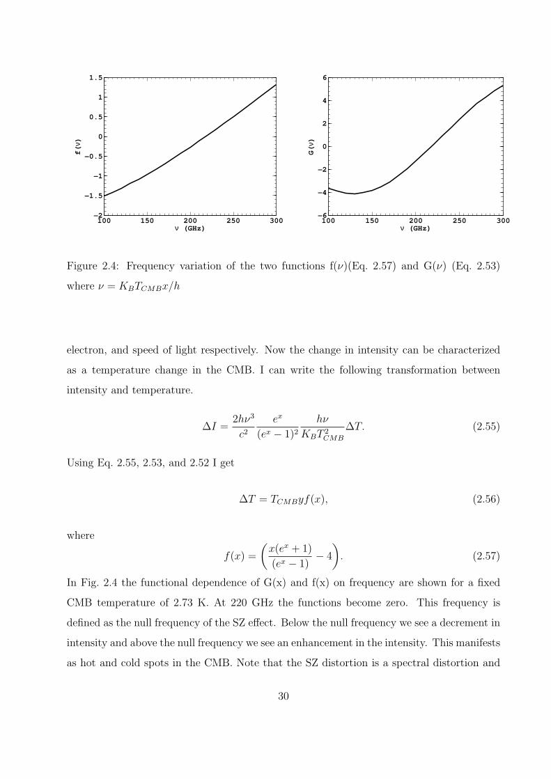
Figure 2.5: SZ spectrum for a Compton y parameter of 0.1. The reference blackbody
spectrum is plotted in solid to show the spectral distortion where i0 = 2.7 × 10⁻¹⁵
ergs/cm2/sec/Hz/Steradian. The typical y parameter for a galaxy cluster is 10−4. At 220
GHz we have the null or the cross-over frequency. The null frequency is a function of the
blackbody temperature only (for the non-relativistic case), and is at 220 GHz for a 2.73 K
blackbody. The null frequency varies and depends on cluster temperature, once we incorpo-
rate the relativistic corrections. In Eq. 2.31 we have neglected terms of O(KBTe/mec2). The
null frequency varies accordingly.
31
so there is a departure from the blackbody spectrum. In Fig. 2.5 the SZ spectrum for a
Compton y parameter of 0.1 is shown with reference to the blackbody spectrum.
The TSZ effect arises from the random thermal motion of the electrons. If there is a finite
velocity of the cluster in the CMB frame there will be an additional Doppler term. This
Doppler anisotropy is called the KSZ distortion. The KSZ distortion is easy to calculate.
Using a relativistic transformation, I can write ν′
= ν(1− β)γ, where γ = 1/√
(1− β2) and
β = v/c, where v is the peculiar velocity of the cluster along the line of sight. For a small
β, I can write ∆T = −Tβτ , (Sunyaev & Zeldovich 1980) where τ = σT∫nedl, is the optical
depth of the cluster. The change in intensity due to the kinetic SZ effect can be obtained
through Eq. 2.55. Substituting for ∆T in Eq. 2.55, I get the change in intensity due to KSZ
effect as,
∆I = −i0 x4ex
(ex − 1)2
vσTc
∫nedl. (2.58)
Note that the kinetic SZ effect comes as a net positive or negative effect depending on the
direction of the peculiar velocity of the cluster with respect to the CMB frame. Unlike the
thermal SZ effect the kinetic SZ effect does not undergo any spectral distortion and is a pure
blackbody.
2.2.4 Cosmology with the SZ Effect
In recent years the SZ effect has become a useful tool in cosmology. Below, I give a brief
description on some of the cosmological uses of the SZ effect.
2.2.4.1 Distance Measurements The SZ effect can be used to determine distances
with combined X-ray observations. As shown in the previous Section, the SZ flux is given
as
∆TSZE ∝∫dlneTe, (2.59)
where terms being usual. The X-ray flux is given as
Sx =
∫dln2
eΛeH , (2.60)
32
where ΛeH is the X-ray cooling function. We further substitute dl = DAdζ, where DA
is the angular diameter distance. Substituting for ne from Eq. 2.59 and 2.60, we get the
approximate angular diameter distance as follows:
DA ∝ (∆T0)2ΛeH0
Sx0T 2e0θc
, (2.61)
where the integral is evaluated along the line of sight through the center of the cluster.
θc is the characteristic angular scale of the cluster. The characteristic scale in the plane
of the sky, θsky, is measured and this serves as an observational proxy for θc. With the
assumption of spherical symmetry the ratio between the two quantities is assumed to be
unity. The second assumption relies on the clumping factor C ≡ 〈n2e〉1/2〈ne〉 being close to one too.
This assumption is violated with the presence of cluster substructures. The measurement of
the angular diameter distance as a function of redshifts can be used to measure distances (see
Carlstrom, Holder, & Reese 2002 for more discussion). With this technique distances can
be measured to high redshifts directly and it is completely independent of other techniques.
Presently the value of Hubble constant measured from combined SZ and X-ray techniques
using data from Chandra, the Owens Valley Radio Observatory (OVRO), and Berkeley-
Illinois-Maryland-Association (BIMA) interferometric array is H0 = 76.93.9−3.4 kms−1 for a
LCDM cosmology (Bonamente et al. 2006). There is a 12% systematic uncertainty associated
with the measurement of the Hubble constant.
2.2.4.2 Gas Mass Fraction Measurement The intercluster medium (ICM) contains
most of the baryonic mass of the cluster in the form of hot X-ray gas (White et al. 1993).
Measuring the gas mass fraction fg in a cluster is a reasonable estimate of the baryonic
mass in the cluster and the universal baryon fraction. A measurement of the baryon fraction
gives an estimate of Ωm with a known value of Ωb, where Ωm and Ωb are the matter density
and baryon density of the universe. The gas mass is directly measured by SZ observations.
If the total gravitating mass is M and the electron temperature is Te then we can either
estimate the total mass (for e.g., from lensing observations) or assume hydrostatic equilibrium
and estimate Te to get the gas mass fraction given by the ratio ∆TSZ/T2e , where ∆TSZ is
the observed SZ decrement or increment. Laroque et al. (2006) determined fg = 0.116 ±
33
0.0050.009−0.016, using data from OVRO and BIMA. The uncertainties in the measurement are
statistical, followed by systematics at 68% confidence.
2.2.4.3 Cluster Cosmology The SZ effect serves as a potential tool for detecting large
samples of galaxy clusters. Since the number density of clusters is a sensitive function of the
underlying cosmology, this enables us to do cosmology with galaxy clusters. See Appendix
C for more discussion. For example, a higher Ωm universe will predict less clusters at high
redshift compared to lower density universe. The cluster number density is also a sensitive
probe of the dark energy parameters (e.g., Mohr 2005). One of the important aspects of
SZ cluster surveys is related to the minimum mass limit of the survey. The mass range to
which a survey is sensitive is determined by the beam size and sensitivity of the instrument
(see Carlstrom, Holder, & Reese 2002). This sets a minimum threshold mass for a flux
limit survey. The mass selection function is relatively uniform (within a factor of 2-3) which
makes SZ a more robust observational tool for fulfilling the completeness criterion compared
to X-rays. Through dedicated SZ surveys like ACT and SPT, cluster number counts can
be observed as a function of redshift. With a large sample of clusters there can be direct
measurements of redshift evolution of cluster number density. This can in principle constrain
cosmological parameters. Although to do precision cosmology the cluster mass needs to be
estimated with better precision. Otherwise there will be systematic bias in measurements of
cosmological parameters due to the inaccuracy of cluster mass measurements. Francis, Bean,
& Kosowsky (2005) show that a 10% systematic bias in mass measurements of galaxy cluster
can incorporate uncertainties that are greater than 1σ level statistical errors. Nagai (2006)
shows from numerical simulation that there exists a tight correlation between integrated
SZ flux from clusters and their corresponding mass which favors the completeness criterion
described above.
The other technique for detecting clusters is through X-ray observations. The current
constraint on cosmological parameters from clusters detected through X-ray observations is
20% for dark energy parameters (Vikhlinin et al. 2009). The two methods have relative
pros and cons. Since the X-ray flux suffers from cosmological dimming where as the SZ
flux is redshift independent, SZ is a better probe for detecting clusters beyond redshift
34
1.0. Also a large region of the sky needs to be observed to obtain a statistically significant
sample to do cluster cosmology. Since X-ray measurements are much more expensive than SZ
observations, it is not possible to obtain a large sample of clusters with X-ray measurements.
The greatest disadvantage of SZ measurements is confusion noise which can lead to a null
detection or a false positive detection. The confusion noise and astronomical contamination
can be disentangled by multi frequency observations (Carlstrom, Holder, & Reese 2002).
Recently Staniszewski et al. (2008) detected four galaxy clusters with SPT by observing 40
square degrees of the southern sky in 95, 159 and 225 GHz. Two of these clusters are at
redshift 0.4. The other two clusters are at redshift ≥ 0.8. Three of these four clusters are
first discovered through SZ observations. Also Hincks et al. (2009) detected ten clusters with
ACT of which two are new cluster candidates. Since clusters probe the highest peaks of the
density field, they can also be used to study cosmological initial conditions. With Gaussian
initial conditions there is a definite prediction of the peak statistics. An observed excess of
high peaks should be a signature of non-Gaussianity (Benson, Reichardt, & Kamionkowski
2001). However there will be contribution from local non-Gaussianity which can confuse the
primordial non-Gaussian signatures.
2.2.4.4 Cluster Peculiar Velocities The KSZ effect is also a powerful tool for cos-
mology since it is the only known way to measure large scale velocity fields. This provides
an opportunity to constrain modified gravity theories with a combined measurement of the
density and velocity fields. However to obtain an accurate peculiar velocity of galaxy clus-
ters to the level of precision cosmology, careful multifrequency observations are required to
separate it from the thermal SZ and primary CMB signal. The first limit on cluster pe-
culiar velocities from KSZ measurements was provided by Holzapfel et al. (1997). With
combined SZ and X-ray data (Sunyaev-Zeldovich Infrared Experiment (SUZIE) and ROent-
gen SATellite (ROSAT)) they measured the peculiar velocities for nearby clusters Abell 2163
(vpec = 490+1370−880 , z = 0.202) and Abell 1689 (vpec = 170+815
−630, z =0.183). The spectrum of
KSZ is degenerate with the CMB and it is intrinsically weak in nature. This makes the
determination of peculiar velocity from clusters extremely difficult. However the mean pe-
culiar velocity on large scales from large sample of clusters is still an interesting route for
35
measuring velocity fields. The uncertainty in Planck’s cluster peculiar velocities is expected
to be between 500-1000 Km/Sec (Aghanim, Gorski, & Puget 2001). With sufficiently large
number of cluster peculiar velocities (of the order of thousands), this velocity error could
still be sufficient to obtain optimistic constraints on dark energy parameters (Bhattacharya
& Kosowsky 2008). However the current status of KSZ is not promising and constraints are
to come from better observations in future.
2.2.4.5 Small Angle SZ In the previous Sections, I discussed the SZ effect from virial-
ized gas in galaxy clusters. However there will be small scale astrophysical effects that can
produce SZ distortions in the CMB (see references in Chapter 1). For the current work we
have estimated the SZ distortion due to energy feedback from active galaxies. In the next
Chapter, I will describe the importance of AGN feedback in theories of galaxy formation
and discuss about how the SZ effect can be used as an effective probe of this process.
36
3.0 FEEDBACK FROM ACTIVE GALACTIC NUCLEI
In this Chapter, I will discuss the importance of AGN feedback and its role on structure
formation. In §3.1 I will describe the observational and theoretical evidences of the role of
AGN feedback on evolution and growth of structures. In §3.2 and 3.3 I will give a brief
description of the possible ways for probing AGN feedback with X-ray, radio, and optical
observations. In §3.4 I will give a brief description of the current theoretical models of AGN
feedback. In §3.5 I will discuss how we can use the SZ effect as a new tool to probe feedback
energy from AGNs.
3.1 ROLE OF AGN FEEDBACK ON STUCTURE FORMATION
3.1.1 The Cooling Flow Problem
One of the hallmarks of X-ray astronomy lies in detecting clusters via the hot X-ray gas
present in the ICM. The first clusters detected in this way were the Perseus and Coma
clusters by the Uhuru satellite (Giacconi et al. 1971; Gursky et al. 1971; Forman et al.
1972). Around 40 clusters were identified as X-ray sources by the mid 1970’s (Gursky
& Schwartz 1977). Clusters are the largest virialized objects in the universe with masses
between 1014 − 1015M. The total gas fraction in clusters is about 16% with about 13% in
the ICM and 3% in galaxies. The rest of the mass consists of dark matter. The gas densities
at the center of galaxy clusters could be as high as 10−1 cm−3 to 10−3 cm−3, which is different
from the cosmic baryon density of 10−8 cm−3. The virial radius of a cluster is defined as
the radius within which the mean density of the cluster is 200 times the critical density
37
(9.4 × 10⁻³⁰gms/cm−3) of the universe. The gas of the cluster is heated by gravitational
infall to temperatures between 1-15 keV (see Peterson & Fabian 2006 for a review). This
comes from the simple assumption of virial equilibrium of KBT ' GMmp/Rv, where M is
the mass of the cluster, Rv is the viral radius (' 1Mpc), mp is mass of proton, G is the
gravitational constant, KB is Boltzmann constant, and T is the temperature of the cluster.
The total X-ray luminosity in galaxy clusters range from 1043 ergs s−1 to 1046 ergs s−1 (see
Peterson & Fabian 2006 for references).
Some of the gas then cools to form stars and the cooling time of the gas is given as
tcool ∝ Tα/ne where T is the temperature of the gas and ne is the gas density (see Fabian
1994 for a review of cooling flows). This comes from the fact that tcool = E/(dE/dt) =
KBT/neΛ(T ), where Λ(T ) is the cooling function (see Peterson & Fabian 2006; Sutherland
& Dopita 1993). The exponent α will depend on the emission mechanisms assumed. The
intracluster gas is densest at the core of the cluster which makes the cooling time at the
core of the cluster to be the shortest. The emission from gas in clusters is mainly due
to thermal Bremsstrahlung process (e.g., Sarazin 1988), and the X-ray luminosity of the
radiation is given as Lx ∝ n2eT
1/2R3v where terms are same as defined above. The other
emission mechanisms are bound-free emission and two-photon emission. Several other line
emissions follow the continuum radiation (Peterson & Fabian 2006 and references therein).
To calculate the X-ray cooling function and the resulting cooling time, an integration of the
energy weighted emission processes is performed (Sutherland & Dopita 1993). Since the gas
density is highest at the center, the X-ray surface brightness at the cluster center tends to
be strongly peaked too. The radiative cooling due to this emission would lead to a subsonic
inflow of gas to maintain the pressure equilibrium. This will lead to a mass deposition rate
of several hundreds of M/yr of cold gas in the cluster center. This is known as the cooling
flow in cluster centers, and clusters that have cooling flows are called cool core clusters.
However recent Chandra and X-MM-Newton observations have shown significant departure
from the standard cooling flow picture (see Peterson & Fabian 2006 for references). The
spectroscopically determined mass deposition rate is found to be few tens of M/yr (Voigt
& Fabian 2004) which is in sharp contrast to the expected cooling flows in galaxy clusters.
These observations suggested the presence of some other mechanisms that could be a viable
38
source for reducing the mass dropout due to cooling.
3.1.2 The LX − T Relation
If we assume the dominant emission mechanism in clusters to be thermal Bremsstrahlung,
then the X-ray luminosity is given as, Lx ∝ n2eT
1/2R3v. For a self similar model (Gravitational
infall) in a virialized cluster (T ∝ M/Rv ∝ R2v) we have Lx ∝ T 2 (Kaiser 1986). However
observations show that Lx ∝ T 3 within the temperature range of 2-8 keV (e.g., Arnaud
& Evrard 1999; Helsdon & Ponman 2000; Voit et al. 2003). This shows a departure from
self-similar model and presence of non-gravitational effects in galaxy clusters.
3.1.3 Cosmic Downsizing
According to standard LCDM cosmology structures form hierarchically. This implies that
bigger structures grow by accretion and merging of smaller structures. Superimposed on
this distribution of dark matter are the baryons which fall into the dark matter potential
well, and eventually undergo radiative cooling to form stars. The larger the structure is,
the longer it takes gas to cool (Rees & Ostriker 1977; Silk 1977) and form stars. This
makes, galaxy formation even more hierarchical than dark matter. However optical and
near infrared observations show that the largest galaxies are in place and the relatively
smaller ones are still forming stars at a redshift of 2.0 (e.g., Glazebrook et al. 2004). This
effect is called “cosmic downsizing” (Cowie et al. 1996). This anti-hierarchical scenario in
galaxy distribution is thought to be the impact of local baryonic physics.
3.1.4 The Missing Piece
Recent observational and theoretical studies have suggested that AGNs could be the missing
piece in this picture. The observed correlation between black hole mass-bulge mass (e.g.,
Gebhardt et al. 2000; Merrit & Ferrarese 2001; Tremaine et al. 2002), and morphological
parameters like the concentration and Sersic index (e.g., Graham & Driver 2007) of the host
galaxies strongly suggest the connection between galaxy evolution and AGN activity. The
39
observed discrepancy in the Lx − T relation suggests an additional heating of 2-3 keV per
particle of the gas in the cluster (e.g., Wu, Fabian, & Nulsen 2000) and AGNs in cluster
centers could be a plausible source for heating the surrounding gas. In recent work on
theoretical models of galaxy evolution with AGN feedback the observed cosmic downsizing
has been reproduced (e.g., Scannapieco & Oh 2004; Granato et al. 2004; Croton et al. 2006;
Cattaneo et al. 2006; Thacker, Scannapieco, & Couchman 2006; Di Matteo et al. 2008).
Parallel connections of the cosmic downsizing effect can also be drawn with the observed
luminosity functions of quasars. Deep X-ray surveys of AGNs show that the spatial density
of AGNs with higher X-ray luminosity peaks at a higher redshift than that of lower luminosity
AGNs (e.g., Ueda et al. 2003). The theoretical simulations show that heating from AGNs
suppresses star formation and hence formation of galaxies (e.g., Scannapieco & Oh 2004; Di
Matteo et al. 2008; Scannapieco, Silk, & Bouwens 2005). The drop in the quasar luminosity
function at lower redshifts has also been reproduced in these simulations (e.g., Scannapieco
& Oh 2004).
Di Matteo, Springel, & Hernquist (2005) carried out simulations of galaxy mergers and
used AGN outflows to produce the observed relation between black hole mass and velocity
dispersion of stars in the center of the host galaxy (MBH − σ) relation. Levine & Gnedin
(2005) combined cosmological simulations with analytic modeling of AGN feedback to put
a constraint on the redshift evolution of the filling factor for AGN outflows. They showed
that the kinetic luminosity of the AGNs should be < 10% of the bolometric luminosity of
the AGN or the intergalactic medium (IGM) would be filled with AGN outflows at z = 0.
Levine & Gnedin (2006) also investigated the impact of AGN feedback on the matter power
spectrum. They found two competing effects that impact the power spectrum. The AGN
outflows move baryons from high to low mass regions, and thus decrease the amplitude of the
matter power spectrum. Also, due to high clustering, AGNs transfer the power from large to
small scales. With a semi analytic model of AGN feedback, Menci et al. (2006) studied the
role of AGN feedback on the color distribution of galaxies from z = 0 to z = 4. They found
that at low redshift AGN feedback increases the number of bright red galaxies. Croton et
al. (2006) investigated the cosmological impact of AGN feedback to explain the low mass
dropout rates in the cooling cores of galaxy clusters and reproduced the exponential cut-off
40
at the bright end of the galaxy luminosity function. Thacker, Scannapieco, & Couchman
(2006) reproduced the observed Lx − T relation in galaxy clusters and showed that AGN
heating is more prominent in galaxy groups.
Evidence for the role of AGN feedback on galaxy evolution has been widely established
through theoretical simulations and X-ray observations of galaxy clusters. However feed-
back models in theories depend on fine tuning of free parameters to match observed results.
Also, no single theoretical model is sufficient in describing all the observed properties. AGN
feedback has not been the only element that plays a role in theories of galaxy formation
and several alternatives have been proposed in this context. To explain the downsizing
effect, Keres et al. (2005) reported a bimodal distribution in the gas accretion phase in
the galaxy distribution that accounted for the quenching of star formation in high mass
galaxies. Stellar and supernova feedback (Pettini et al. 2001) have been other suggested al-
ternatives for quenching star formation. Khochfar & Ostriker (2008) explained the quenching
of star formation by including more sophisticated model of gas physics. In the context of
non-gravitational heating source in clusters, other alternatives including cosmic rays (e.g.,
Colafrancesco, Dar, & DeRujula 2004), supernova outflows (e.g., Silk et al. 1986), and exotic
events like interactions with dark matter (e.g., Totani 2004) have been addressed by different
authors. Another alternative to AGN feedback has been thermal conduction (Zakamska &
Narayan 2003). The theory involves conducting heat from the outskirts of the galaxy to the
core. In the following Sections, I will describe the multifrequency observations and some
theoretical models of AGN feedback.
3.2 X-RAY OBSERVATIONS OF AGN FEEDBACK
Modern X-ray telescopes are sensitive to X-ray energies ranging from 0.1 keV-10 keV (see Mc-
Namara & Nulsen 2007 for a review). Results from X-ray observations show that AGNs at the
center of galaxy clusters are pouring huge amount of energy into the gas in the intra-cluster
medium. AGN activity on the X-ray gas in clusters was first noted by Branduardi-Raymont
et al. (1981) in Perseus with the Einstein satellite. Other observations with Rosat were done
41
by, e.g., Boehringer et al. (1993), Huang & Sarazin (1998). However the explanation of
AGN activity was not fully understood until observations of the Chandra and XMM-Newton
satellites. There has been observational evidence of three dozen cD galaxies in clusters and
a similar number of giant Ellipticals (gE) harboring cavities or bubbles in their X-ray halos
(e.g., McNamara et al. 2000; Heinz et al. 2002). It is believed that the cavities are produced
by AGN outflows displacing the X-ray gas in the intracluster medium. Cavity systems in
clusters can also vary in size from 1 kpc to 200 kpc (e.g., Forman et al. 2005). These X-ray
cavities are associated with radio lobes and a correlation exists between radio luminosity
and cavity power (e.g., Dunn & Fabian 2006). An interesting discovery from Chandra is the
X-ray cavity that is not associated with radio lobes (McNamara et al. 2001; Fabian et al.
2002). These cavities are called ghost cavities and are believed to be aging radio relics that
have broken free from the jets (see McNamara & Nulsen 2007 for discussion). The work
required to inflate cavities against the pressure is around 1055 ergs in gEs and about 1061
ergs in rich clusters (e.g., Rafferty et al. 2006). The displaced gas mass from these cavities
could be 1010M in an average cluster system such as Abell 2052 (e.g., Blanton et al. 2001)
but could be as high as 1012M in powerful outbursts as seen in MS0735.6+7421 and Hydra
A (see McNamara & Nulsen 2007 for references).
3.3 RADIO AND OPTICAL OBSERVATIONS
3.3.1 Radio Observations
The other major tool to study AGN feedback is through radio observations. Radio observa-
tions offer a view of the extent of AGN interaction, provide insights into outburst history,
and give clues about source geometry, whereas from X-ray observations we get a direct view
of the physical state of the gas, a measure of energies injected by outbursts, and a view of the
gas motion (e.g., Vrtilek et al. 2008). Radio jets are the main mechanism by which energy
is carried from AGNs. Burns (1990) studied the multifrequency properties of cD galaxies
in clusters using radio data from 6 cm VLA maps and X-ray data from the Einstein IPC.
42
The results showed significant correlation between x-ray cooling cores and radio emission
and morphology. As discussed before, the absence of sufficient cooling led to the hypothesis
of AGN activity at the center of the cluster. It is now shown by, e.g., Dunn, Fabian, &
Taylor (2005) and Dunn & Fabian (2006), that cooling core clusters harbor radio bubbles
that are associated with AGN heating. Dunn & Fabian (2006) used the VLA and the Aus-
tralian Telescope Compact Array (ATCA) to show that the radio morphology of some of
these bubbles are bilobed with an average bubble size of 1 − 2 kpc. Birzan et al. (2004)
studied a large sample of X-ray cavities and radio bubbles in clusters and groups and ob-
tained the PV energy of the cavity and their ages. Best et al. (2006a) estimated the heating
rate from radio loud AGNs in galaxy clusters to be H = 1021.4(MBH/M)1.6 W, by using
data from NVSS and Faint Images of the Radio Sky at Twenty centimeters (FIRST). Best
(2007) showed that the heating from radio loud AGNs balances the cooling flow in elliptical
galaxies within groups and clusters. However, it is important to note that the cooling flow
problem is still not understood theoretically. AGN feedback is a possible explanation but
there is still enough room in theory for cold gas to condense into filaments and make its way
to the cluster center. At even lower radio frequencies Giacintucci et al. (2008) studied radio
morphology of galaxy cluster AWM4 with the Giant Meter wave Radio telescope (GMRT)
and found evidence of AGN feedback associated with the central radio source.
3.3.2 Optical Observations
Although most of the AGN activity in clusters is associated with radio loud quasars there
has been substantial evidence of radio quiet quasars being effective enough in influencing
their environments. The broad absorption line (BAL) quasars (Turnshek 1984) can affect
their environments by producing strong winds (e.g., Fabian 1999). The current fraction of
BAL quasars among the radio quiet population may be as high as (22 ± 4)% (e.g., Hewett
& Foltz 2003; Reichard et al. 2003). Gallagher et al. (2006) studied the X-ray properties
of BAL quasars and found evidence of strong outflow. Chartas et al. (2007) also studied
X-ray properties of BAL quasars and determined the fraction of the total bolometric energy
released by the quasars into the intergalactic medium (IGM). Although there have been
43
various observational probes of the interaction of AGNs with their environments, it is fair
to say that there is not a well established unified theory that will be sufficient to model the
outflows and heating mechanisms in AGNs. In the next Section, I will describe some aspects
of theoretical modeling of heating of cluster environments by AGNs. These theoretical
models are not relevant in describing outflows from radio quiet quasars but assume the radio
loud mode inherently. Different models associated with the generation of quasar winds in
BAL quasars are described in deKool (1997).
3.4 THEORETICAL MODELS OF AGN FEEDBACK
I will discuss three representative models for AGN heating (see McNamara & Nulsen for a
review).
3.4.1 Cavity Heating
From X-ray observations of galaxy clusters it has been shown that X-ray cavities are formed
due to AGN activity. The total energy required to inflate the cavity is given by H = E+PV ,
where H is defined as the enthalpy of the system, E is the internal energy, and PV is the
work required to displace the X-ray emitting gas. If the radio lobe within the X-ray cavity
is filled with ideal gas (with a ratio of constant specific heat (γ)) we can write the total
enthalpy of the system as H = PVγ−1
+ PV = γγ−1
PV . For different values of γ there will be
different enthalpy profiles of the gas inside the cavity. As a buoyant cavity raises through
the cluster atmosphere (e.g., Reynolds et al. 2002; Bruggen & Kaiser 2002) some X-ray gas
moves inward to fill the space. If the cavity rises a distance δR and if M is the mass of the
displaced gas, we can write the change in potential energy as
δU = MgδR = −MdP
ρ= −V δP, (3.1)
where g is acceleration due to gravity. Here we used the assumption of hydrostatic equilib-
rium. Using the first law of thermodynamics expressed in terms of enthalpy, we can write
44
an isentropic (adiabatic) process as
dH = TdS + V dP = V dP. (3.2)
Thus we see that the kinetic energy created in making the bubble rise is equal to the loss of
its enthalpy. The kinetic energy dissipates due to the viscosity of the surrounding gas in the
form of heat. Using Eq. 3.2 we can write the enthalpy of a cavity as
H = H0(P/P0)(γ−1)/γ, (3.3)
where we have used the adiabatic equation of state PV γ = constant to do the integral. H0
is the initial enthalpy of the cavity and P0 is the initial pressure of the surrounding gas. If
the mean power injected by an AGN as cavity enthalpy is Lb we can write the mean heating
rate per unit volume averaged over a sphere of radius R as (see McNamara & Nulsen 2007
for more discussion)
Πb = − Lb4πR2
d
dR
(P
P0
)(γ−1)/γ
. (3.4)
This model is described as the 1D effervescent heating model of AGN feedback (e.g., Begel-
man 2001; Roychowdhury et al. 2004; Guo, Peng, & Ruszkowski 2008). 3D simulations
involving anisotropic cavity heating have been undertaken by Quilis et al. (2001) and Dalla
Vecchia et al. (2004).
3.4.2 Shock Heating
Voit & Donahue (2005) have observed several clusters which have peaky entropy profiles
in the centers and do not harbor strong radio sources. These samples of clusters show no
evidence of AGN activity. They suggested that the high entropy signature is due to powerful
shocks that were generated by AGNs in the past. Voit & Donahue (2005) showed that
the entropy profiles of the clusters are consistent with shock heating within tens of kpc
of the cluster center. In the outskirts there is more agreement with enthalpy heating (see
McNamara & Nulsen 2007 and references therein). Shock heating tends to play an important
role close to the AGN (e.g., Fabian et al. 2005). Shocks are believed to be generated due
to instabilities in the accretion disc. The entropy created by dissipation of shock fronts is
45
proportional to the cube of the shock strength characterized by pressure instability (Landau
& Lifshitz 1987). The equivalent heating rate is
Πs =(γ + 1)
12γ2
ωp2π
(δP
P
)3
, (3.5)
(McNamara & Nulsen 2007), where ωp is the interval between shocks. In real observations
the generation of shocks could be aperiodic. Evidence of weak shocks has been observed in
some clusters (e.g., Forman et al. 2005; McNamara et al. 2005).
3.4.3 Sound Damping
Fabian et al. (2003) showed that viscous damping of sound waves generated by repeated
outbursts of AGN may produce a significant amount of heating (see McNamara & Nulsen
2007 for references). The heating rate from sound damping can be written as (Landau &
Lifshitz 1987)
Πd =
[2µ
3ρ+
(γ − 1)2κT
2γP
]ω2ρ
γ2
(δP
P
)2
, (3.6)
where ρ, T , P , γ, κ, ω, and µ are density, temperature, pressure, ratio of specific heats of
the gas, thermal conductivity, angular frequency, and viscosity, respectively.
In practice the non-gravitational energy coming from an AGN is propagated within
the cluster environment by a combination of the three mechanisms described above. By
comparing the heating rates, it is now known that the ratio of shock heating to sound
damping decreases with radius. This makes shock heating confined to the regions near
the AGN. The comparison of the theoretical rates show that cavity heating tends to be
more centrally concentrated compared to shock heating but in practice cavity heating stays
ineffective inside the radius where the cavity is formed. This makes shock heating the most
centrally concentrated heating mechanism near the AGN. Cavity heating takes over the role
outside the cavity (Voit & Donahue 2005). It appears that the mechanism of heating varies
with radius and no single process can be considered the most significant.
46
3.5 THE SZ EFFECT AS A PROBE
It is also important to note that the overall level of feedback will depend on the source type.
If it is within the radio-quiet mode (BAL quasar), the outflow will be dominated by winds.
If it is in the jet mode, there will be shock heating and cavity heating. In clusters we mostly
tend to observe the jet mode of feedback, and earlier studies claimed that radio loud AGNs
tend to be found in dense environments compared to radio quiet ones (e.g., Ellingson, Yee,
& Green 1991). However later studies showed that radio quiet AGNS are found in the same
proportions as radio loud ones in galaxy clusters (e.g., Bahcall et al. 1997; McLure & Dunlop
2001). Theoretically a ‘two-mode’ model for AGN feedback has been recently proposed by
Sijacki et al. (2007). These two modes are termed as “quasar mode” and “radio mode”.
The quasar mode corresponds to high accretion stages of the black hole with a radiatively
efficient thin disc accretion (Shakura & Sunyaev 1973). The radio mode corresponds to low
accretion phases of a black hole with geometrically thick radiatively inefficient accretion.
The quasar mode radiates energy isotropically and the radio mode transfers energy in the
form of anisotropic jets.
In our theoretical modeling and simulation work of AGN feedback in the next two Chap-
ters, we have assumed spherical symmetry which will mostly be representative of the quasar
mode of feedback. We note that although the transport mechanisms and the AGN types will
be extremely important in describing AGN activity, the amplitude of feedback energy is the
most relevant quantity in cosmological applications. The SZ effect which is sensitive to the
total amount of feedback energy from the AGN will hence give a correct order of magnitude
estimate of the signal. Since the SZ effect is an effective tool for studying accumulations
of hot gas in the universe, regardless of the redshift of the source producing the hot gas,
we propose to study the hot gas in AGN environments by studying its SZ distortion in the
CMB. This SZ signal will be in addition to the SZ signal that we expect from virialized gas
in galaxy clusters. This gives us a new observational tool to study feedback energy from
active galaxies and put constraint on theories of galaxy formation.
47
4.0 ANALYTIC MODEL OF AGN FEEDBACK
In this Chapter, the calculation of SZ distortion from analytic modeling of AGN feedback
is discussed. We have assumed a one dimensional Sedov-Taylor model of energy ejection
and we analytically calculate the y distortion from it. We obtain the power spectrum of y
distortion in multipole space and show its dependence on some of the free parameters in
the model. Finally, we calculate the observational signal for SZ distortion from the power
spectrum using a Gaussian beam. In §4.1 the Sedov-Taylor model and the equations used
for modeling the feedback process are discussed. In §4.2 the mathematical formalism and
the derivation of the y distortion are shown. In §4.3 the method for calculating the power
spectrum is described. In §4.4 the dependence of the power spectrum on various parameters
of the model is shown, and finally, in §4.5 the calculation of the observational signal from
our model is illustrated.
4.1 AGN OUTFLOW MODEL
In our analytic model of AGN feedback we assume that an AGN injects a substantial amount
of energy into the surrounding gas while it is active. Following Scannapieco & Oh (2004),
we assume the black hole powering the AGN shines at its Eddington luminosity and returns
around 5% of this energy to the galactic gas, eventually disrupting its own fuel source after
a dynamical time of the cold gas surrounding the black hole, tdyn ' 4 × 10⁷(1 + z)−3/2
yr (Barkana & Loeb 2001). The Eddington luminosity is the maximum luminosity beyond
which radiation pressure prevents gas accretion. The Eddington luminosity can be evaluated
by equating the radiative repulsive force on a free electron to the gravitational attractive
48
force on an ion in the plasma (Eddington 1926). The Eddington luminosity is given by
LED = (4πGcMBHµemp)/σT = 1.45×1046(MBH/108M) ergs/s. The dynamical time comes
from the following ratio MBH/(dMBH/dt). Using MBH = ε0L/c2 we can write the dynamical
time as tdyn ' 4×10⁷(ε0/0.1)(L/LED)−1 yr, where ε0 is the radiative efficiency. The feedback
efficiency factor is assumed to be 5% (Scannapieco & Oh 2004). This is consistent with the
theoretical estimate of Wyithe & Loeb (2003), where they assumed a self-regulatory accretion
model and showed that (5%) is the limit within which a self-regulatory growth is achieved.
The duration of the blast, tdyn, is much shorter than the expansion time of the resulting
bubble of hot gas (on the order of 109 years). Therefore, we assume an instantaneous point
source injection of energy into the intergalactic medium. The total energy output is just the
product of the luminosity, the efficiency factor (εk), and the duration (tdyn = 5×10⁷(1+z)−3/2
years) of the explosion. The Mbh-σ relation (Merritt & Ferrarese 2001; Tremaine et al.
2002)and the vc − σ relation (Ferrarese 2002; Shields et al. 2003) can be used to connect
the black hole luminosity with the mass of the host halo where σ and vc are the velocity
dispersion and the circular velocity of the host halo respectively.
MBH = (1.66± 0.32)× 108M( σ
200kms−1
)4.58±0.52
. (4.1)
log10
( vc300kms−1
)= (0.84± 0.09)log10
( σ
200kms−1
)+ (0.55 + 0.19). (4.2)
Combining Eq. 4.1 and 4.2 we get the following relation between black hole mass and circular
velocity
MBH = 1.4× 10⁸MF( vc
300kms−1
)5
, (4.3)
where F is a constant free parameter taken as 0.6 (Scannapieco & Oh 2004). The circular
velocity can be written as
vc = 140kms−1M1/312 (1 + z)1/2, (4.4)
where M12 ≡Mhalo/1012M. Using Eq. 4.3 and 4.4 we obtain the total energy injected from
an AGN turning on at redshift z in a halo of mass Mhalo as a function of Mhalo and z. The
relation is given as
E = εkMBHc2tdyn = 0.06M
5/312 (1 + z), (4.5)
49
where εk = 0.05 and c is the speed of light. E is shown in units of 1060 ergs. For simplicity,
we assume that after the energy injection, a hot bubble evolves adiabatically and expands
into a medium of uniform overdensity. The one-dimensional Sedov-Taylor solution is used to
model the radius and temperature of the region contained by the blast wave (Scannapieco
& Oh 2004).
The Sedov-Taylor model (e.g., Shu 1992) describes the theory of strong point like ex-
plosion in a uniform medium. Let us consider an amount of energy E being released into
a static medium that has uniform density ρ1. Let t be the time considered after the initial
explosion. To know, how the radius (rsh) of the energy ejecta (blast wave) grows in time we
consider a dimensionality analysis. Let us consider r0 to be a dimensionless quantity such
that
r0 = rshtlρm1 E
n. (4.6)
This gives the following relations involving l, m, and n. 1 − 3m + 2n = 0, l − 2n = 0 and
m+ n = 0. Using these relations we have
rsh = r0(Et2/ρ1)1/5. (4.7)
The velocity of the blast wave will be
Ush =drshdt
=2
5
rsht. (4.8)
In a frame fixed to the center of the explosion, the Rankine Hugoniot jump condition gives
relation between the pre shock (denoted by suffix 1) and post shock (denoted by suffix 2)
quantities.
ρ2 = (γ + 1
γ − 1)ρ1, (4.9)
P2 = (2
γ + 1)ρ1U
2sh, (4.10)
where ρ and P are density and pressure of the medium, γ = 5/3, and r0 = 1.17 (Shu 1992).
Using the relation P2 = T2ρ2KB/m2, where m2 is the mean particle mass behind the shock,
we use Eq. 4.9 and 4.10 to get the expression for the post shock temperature
T2 = 3m2U2sh/16KB. (4.11)
50
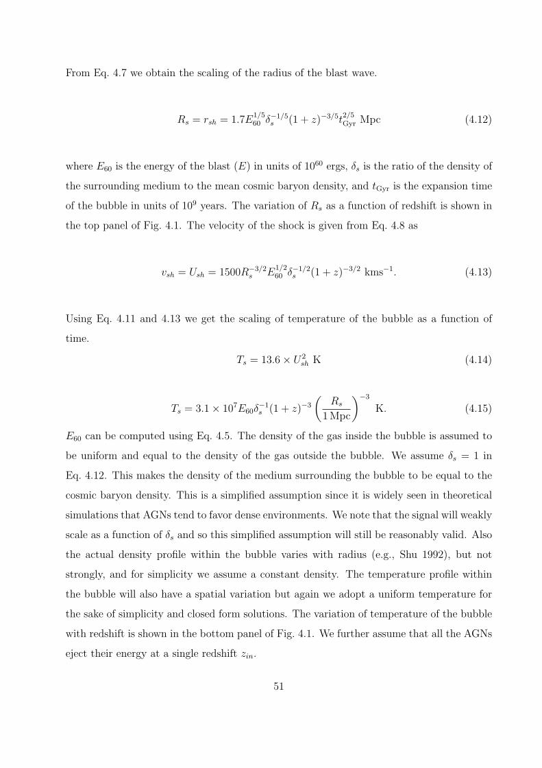
From Eq. 4.7 we obtain the scaling of the radius of the blast wave.
Rs = rsh = 1.7E1/560 δ
−1/5s (1 + z)−3/5t
2/5Gyr Mpc (4.12)
where E60 is the energy of the blast (E) in units of 1060 ergs, δs is the ratio of the density of
the surrounding medium to the mean cosmic baryon density, and tGyr is the expansion time
of the bubble in units of 109 years. The variation of Rs as a function of redshift is shown in
the top panel of Fig. 4.1. The velocity of the shock is given from Eq. 4.8 as
vsh = Ush = 1500R−3/2s E
1/260 δ
−1/2s (1 + z)−3/2 kms−1. (4.13)
Using Eq. 4.11 and 4.13 we get the scaling of temperature of the bubble as a function of
time.
Ts = 13.6× U2sh K (4.14)
Ts = 3.1× 10⁷E60δ−1s (1 + z)−3
(Rs
1 Mpc
)−3
K. (4.15)
E60 can be computed using Eq. 4.5. The density of the gas inside the bubble is assumed to
be uniform and equal to the density of the gas outside the bubble. We assume δs = 1 in
Eq. 4.12. This makes the density of the medium surrounding the bubble to be equal to the
cosmic baryon density. This is a simplified assumption since it is widely seen in theoretical
simulations that AGNs tend to favor dense environments. We note that the signal will weakly
scale as a function of δs and so this simplified assumption will still be reasonably valid. Also
the actual density profile within the bubble varies with radius (e.g., Shu 1992), but not
strongly, and for simplicity we assume a constant density. The temperature profile within
the bubble will also have a spatial variation but again we adopt a uniform temperature for
the sake of simplicity and closed form solutions. The variation of temperature of the bubble
with redshift is shown in the bottom panel of Fig. 4.1. We further assume that all the AGNs
eject their energy at a single redshift zin.
51
00.511.522.50
0.5
1
1.5
2
2.5
3
z (redshift)
Rs (Mpc)
00.511.522.510
5
106
107
108
z (redshift)
Ts (K)
Figure 4.1: The radius (top panel) and temperature (bottom panel) of the bubble is shown
as a function of redshift. The profiles are shown for a halo mass of 1012M and δs = 1. The
profiles correspond to Eq. 4.12 and 4.15.
52
4.2 CALCULATION OF THE Y DISTORTION
The y distortion in Eq. 2.54 is given as the integrated line of sight pressure of the gas in
the bubble. To calculate the y distortion we assume the bubble to be spherically symmetric.
With the assumption of spherical symmetry, constant temperature, and constant number
density of electrons inside the hot bubble surrounding the AGN, the y-distortion y(θ) on the
sky will be azimuthally symmetric, depending only on the angle θ between the bubble center
and a particular line of sight. The line of sight distance is given as l = 2(R2s − D2
Aθ2)1/2,
where Rs is the radius of the bubble and DA(z) is the angular diameter distance to redshift
z. We can write the y distortion as (after integrating Eq. 2.54)
y(θ) =4σTKB
mec2TeneRs
[1− D2
Aθ2
R2s
]1/2
. (4.16)
The profiles of y distortion at redshifts 1.0 and 3.0 are shown in Fig. 4.2. The y distortion
profiles in galaxy clusters follow an isothermal β profile. The profiles in galaxy clusters are
shown in Appendix D. With a small angle approximation we can write the angular Fourier
transform of the y-distortion as (cf. Peebles 1980; see Appendix D for derivation)
yl =8πKBσTmec2
TeneRs
∫θdθ
[1− D2
Aθ2
R2s
]1/2
J0
[(l +
1
2
)θ
], (4.17)
where J0 is the cylindrical Bessel function of order 0. With further simplifications we get,
yl(m, z) =8πKBσTmec2
TeneR3s
D2A
∫ 1
0
(1− s2)µJν(bs)sν+1ds, (4.18)
where s2 = D2Aθ
2/R2s, µ = 1/2,, ν = 0, and b = (l + 1/2)Rs/DA. This integral can be
performed analytically (Gradshteyn & Ryzhik 1980) and is given as
I = 21/2Γ(3/2)b−3/2J(b). (4.19)
From Eq. 4.18 and 4.19 we get,
yl(M, z) =16σTKBTeneR
3/2s
D1/2A
(π
2l + 1
)3/2
J3/2
[(l +
1
2
)Rs
DA
]. (4.20)
We note that Te and Rs depend on both the halo mass M and the redshift z, and ne depends
on z. Equation 4.20 gives the analytic form of the y distortion in multipole space.
53
0 0.2 0.4 0.6 0.8 17
7.2
7.4
7.6
7.8
8
8.2
8.4
8.6
8.8
9x 10
−10
θ (arcminutes)
y(
θ)
0 0.05 0.1 0.150.5
1
1.5
2
2.5
3
3.5
4x 10
−7
θ (arcminutes)
y (
θ)
Figure 4.2: Profile of y distortion within the bubble radius at redshift 1.0 (top panel) and
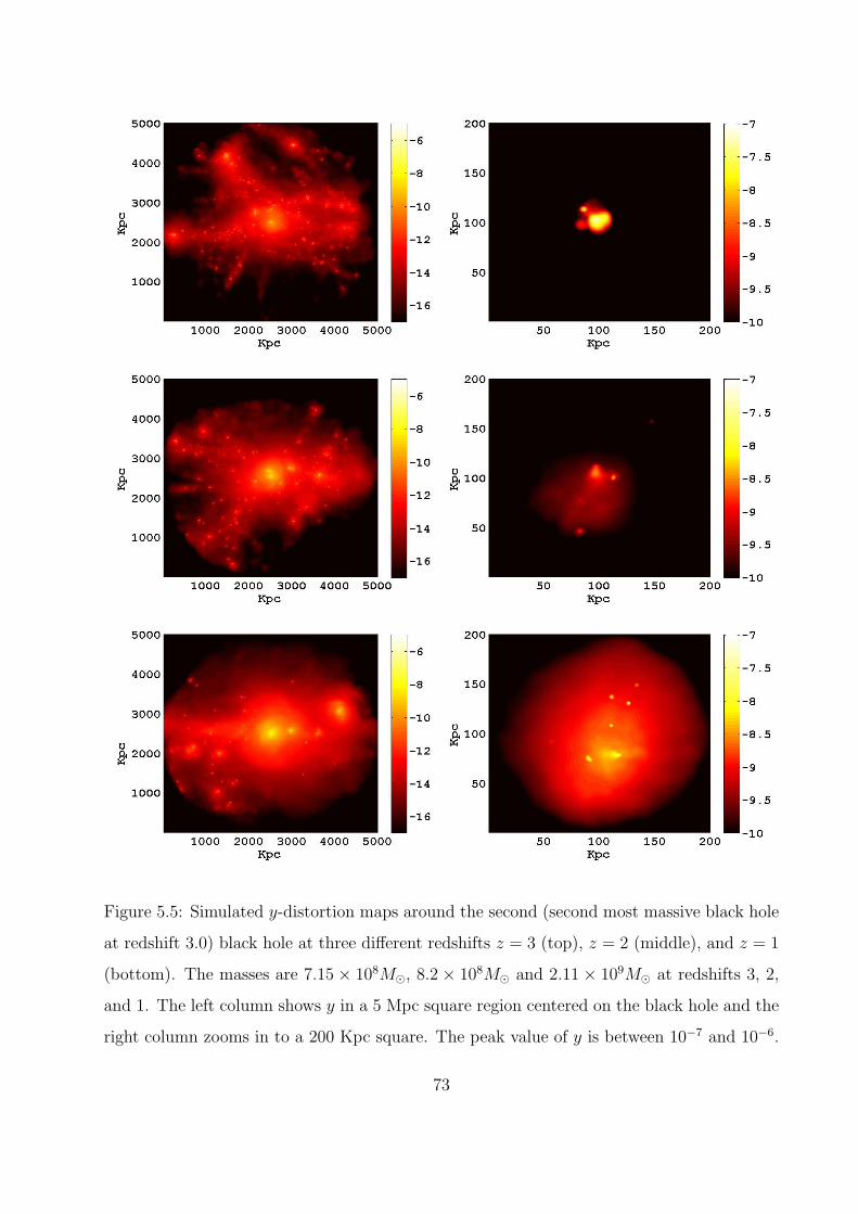
redshift 3.0 (bottom panel). The size of the bubble is smaller (see top panel of Fig. 4.1), but
the temperature of the bubble is higher (bottom panel of Fig. 4.1) at higher redshift. This
makes the signal higher at higher redshift. The halo mass is assumed to be 1012M, with
δs = 1.
54
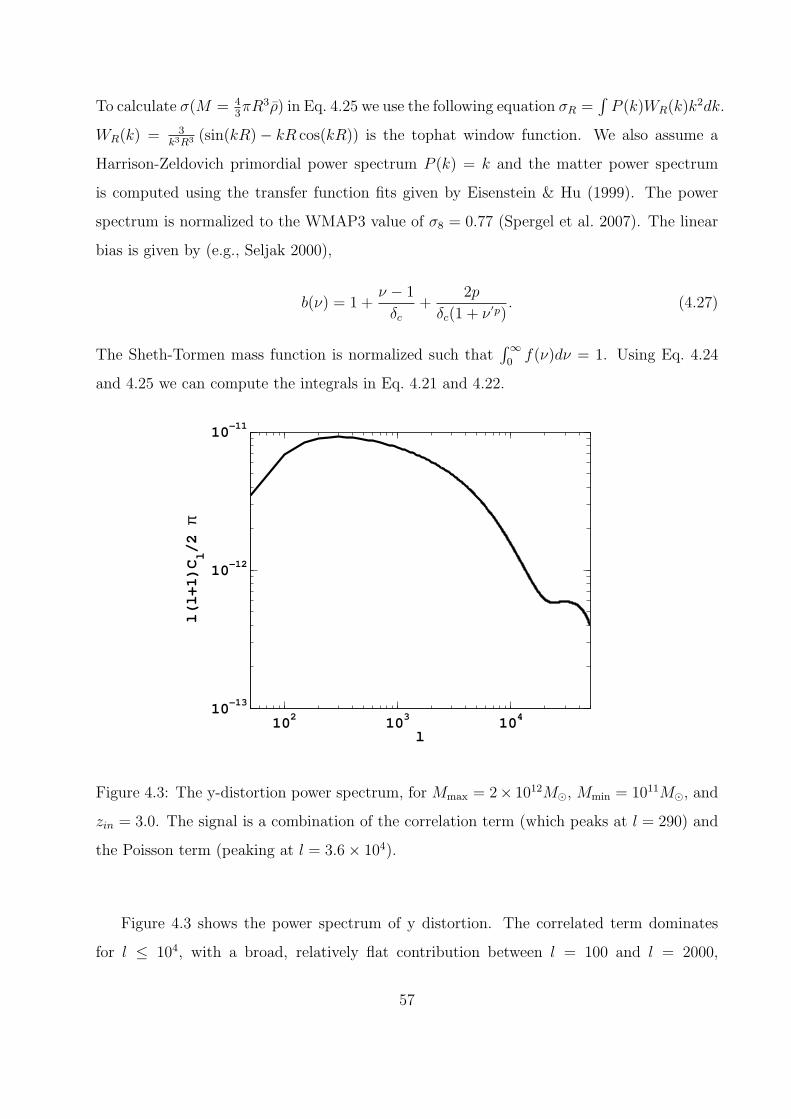
4.3 CALCULATION OF THE POWER SPECTRUM
The y-distortion on the sky can be conventionally expanded in terms of the spherical harmon-
ics as y(n) =∑
lm almYlm(n). The angular power spectrum is then obtained as Cl = 〈|alm|2〉,an ensemble average over the coefficients. The power spectrum has two components (e.g.,
Cole & Kaiser 1988, see Cooray & Sheth 2002 for a review), Cyyl = Cp
l +Ccl , where Cp
l is the
contribution from Poisson noise of the random galaxy distribution, and Ccl comes from the
correlation between galaxies. The two terms are given as (e.g., Komatsu & Kityama 1999;
Majumdar, Nath, & Chiba 2001)
Cpl =
∫ zin
0
dzdV
dz
∫ Mmax
Mmin
dMdn(M, zin)
dM|yl(M, z)|2 , (4.21)
Ccl =
∫ zin
0
dzdV
dzPm(kl(z))
(∫ Mmax
Mmin
dM Φl(M, z)
)2
, (4.22)
where
Φl(M, z) =dn(M, zin)
dMb(M, zin)yl(M, z), (4.23)
kl(z) ≡ l/DA(z) is the wave number corresponding to the multipole angular scale l at redshift
z, dV/dz is the comoving volume element, dn(M, z)/dM is the differential mass function,
Pm(k, z) is the matter power spectrum, and b(M, z) is the linear bias factor. The expression
for the correlated piece uses the Limber approximation (see Peebles 1980). The upper limit
of the redshift integral zmax is assumed to be the redshift (zin) at which all the AGNs eject
there energy. As mentioned before (end of §4.1) we use a simplified assumption in which all
the AGNs eject their energy at a single redshift.
We used the following quantities to compute the power spectra defined in Eq. 4.21 and
4.22. The comoving volume term is given in Hogg (1999) as
dVcdΩdz
=D3H
E(z)
(∫ z
0
dz′
E(z′)
)2
, (4.24)
where E(z) = (Ωm(1 + z)3 + ΩΛ)1/2 and DH = 3000h−1Mpc is the Hubble distance. Ωm
and ΩΛ are cosmological parameters defined in Table 1.1. Throughout the work we assume
a standard LCDM cosmology with Ωm = 0.31, Ωb = 0.044. To calculate the power spectrum
55
of fluctuations we need to find the number density of AGNs since we need to integrate over
the mass function. To do this, we associate the number density of AGNs with the number
density of dark matter halos at redshift zin when the AGNs eject their energy, and we use the
Sheth-Tormen function (f(ν)) (Sheth & Tormen 1999; Seljak 2000) to calculate the number
density of halos. We also assume a halo mass to black hole mass ratio of 104, roughly a factor
of 500 from the bulge-black hole mass ratio (e.g., Marconi & Hunt 2003) and a factor 20
from the bulge-halo mass ratio (e.g., Dubinski, Mihos, & Hernquist 1996). If the minimum
mass black hole needed to power an AGN is taken as ' 107M, the minimum relevant halo
mass is around ' 1011M, which we take as a lower mass cut-off for the halos. We note
that the effect we are calculating is from field AGNs (corresponding to the mass limits of
halos described above) and not of AGNs that reside in cluster centers. In Chapter 5, we will
use numerical simulations to show the effect of AGN feedback in galaxy groups (mass of the
largest halos in the simulation corresponds to group size halos) and how it will contribute
to the SZ signal. After we integrate the Sheth-Tormen function f(ν) over the solid angle we
get the following equation (Seljak 2000):
dn
dM= 4πf(ν)dν
ρ
M. (4.25)
f(ν) =(1 + ν ′p)ν ′1/2e−ν
′/2
ν,
ν ′ = aν,
where, a = 0.707, p = 0.3
ν = (δc
σ(M)D(z))2,
ρ is the mean density of the universe and δc is the value of a spherical overdensity at which
it collapses at a given redshift z. For a de-Sitter model δc = 1.68. To compute the linear
growth factor D(z) we assume the following form (Dodelson 2002)
D(z) = 2.5
(∫ 1/(1+z)
0
da
(Ωma3 + ΩΛ)1.5
)Ωm(Ωm(1 + z)3 + ΩΛ)1/2 (4.26)
56
To calculate σ(M = 43πR3ρ) in Eq. 4.25 we use the following equation σR =
∫P (k)WR(k)k2dk.
WR(k) = 3k3R3 (sin(kR)− kR cos(kR)) is the tophat window function. We also assume a
Harrison-Zeldovich primordial power spectrum P (k) = k and the matter power spectrum
is computed using the transfer function fits given by Eisenstein & Hu (1999). The power
spectrum is normalized to the WMAP3 value of σ8 = 0.77 (Spergel et al. 2007). The linear
bias is given by (e.g., Seljak 2000),
b(ν) = 1 +ν − 1
δc+
2p
δc(1 + ν ′p). (4.27)
The Sheth-Tormen mass function is normalized such that∫∞
0f(ν)dν = 1. Using Eq. 4.24
and 4.25 we can compute the integrals in Eq. 4.21 and 4.22.
102
103
104
10−13
10−12
10−11
l
l(l+1)Cl/2
π
Figure 4.3: The y-distortion power spectrum, for Mmax = 2× 10¹²M, Mmin = 1011M, and
zin = 3.0. The signal is a combination of the correlation term (which peaks at l = 290) and
the Poisson term (peaking at l = 3.6× 10⁴).
Figure 4.3 shows the power spectrum of y distortion. The correlated term dominates
for l ≤ 104, with a broad, relatively flat contribution between l = 100 and l = 2000,
57
corresponding to angular scales from 2 degrees down to 5 arcminutes (the angular scales on
which large scale structure is evident). The Poisson term contributes the secondary peak
around l = 3 × 10⁴, at an angular scale of around 20′′ (the characteristic separation of
galaxies). In this case Mmax = 2×10¹²M, Mmin = 1011M, and zin = 3.0. The y-distortion
power spectrum can be converted to an effective temperature power spectrum at a given
frequency via Eq. 2.56 and 2.57.
4.4 PARAMETER DEPENDENCE OF THE POWER SPECTRUM
102
103
104
10−14
10−13
10−12
10−11
l
l(l+1)Cl/(2
π)
102
103
104
10−13
10−12
10−11
10−10
l
l(l+1)Cl/2
π
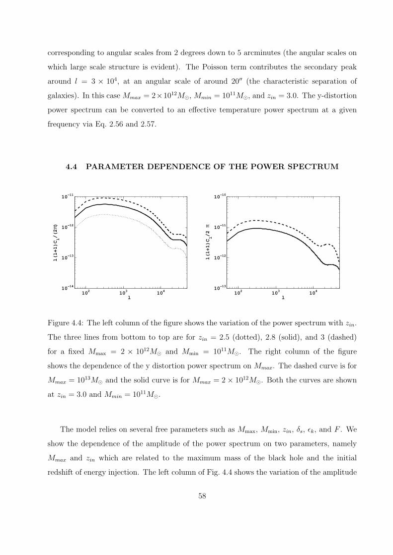
Figure 4.4: The left column of the figure shows the variation of the power spectrum with zin.
The three lines from bottom to top are for zin = 2.5 (dotted), 2.8 (solid), and 3 (dashed)
for a fixed Mmax = 2 × 10¹²M and Mmin = 1011M. The right column of the figure
shows the dependence of the y distortion power spectrum on Mmax. The dashed curve is for
Mmax = 1013M and the solid curve is for Mmax = 2× 10¹²M. Both the curves are shown
at zin = 3.0 and Mmin = 1011M.
The model relies on several free parameters such as Mmax, Mmin, zin, δs, εk, and F . We
show the dependence of the amplitude of the power spectrum on two parameters, namely
Mmax and zin which are related to the maximum mass of the black hole and the initial
redshift of energy injection. The left column of Fig. 4.4 shows the variation of the amplitude
58
of the power spectrum as a function of zin. The three lines from bottom to top are for zin =
2.5, 2.8, and 3.0 respectively. The right column of Fig. 4.4 shows the variation of the power
spectrum amplitude with Mmax (or MBH thereof). From Fig. 4.4 we see that change in zin
from 3 to 2.5 reduces the power spectrum by roughly a factor of 2, with the Poisson term
and the correlated term being affected equally. The dependence on maximum mass Mmax is
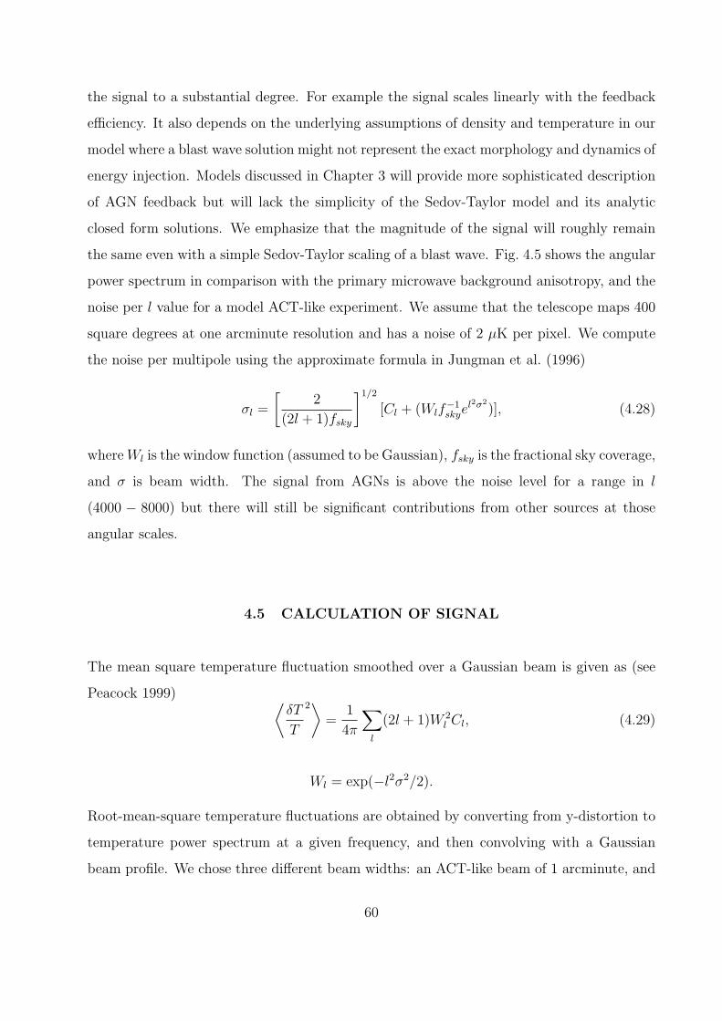
Figure 4.5: The y-distortion power spectrum with reference primary anisotropy (dotted line)
and the noise level per l value (dashed line) for an ACT-like model experiment covering 400
square degrees with 1 arcminute resolution and a pixel noise of 2 µK (target pixel noise for
ACT in the original proposal). In this case Mmax = 2 × 10¹²M, Mmin = 1011M, and
zin = 3.0.
relatively weak: the power spectrum amplitude increases only by a factor of around 60% if the
maximum mass is increased by a factor of 5. The other parameters in the model can also alter
59
the signal to a substantial degree. For example the signal scales linearly with the feedback
efficiency. It also depends on the underlying assumptions of density and temperature in our
model where a blast wave solution might not represent the exact morphology and dynamics of
energy injection. Models discussed in Chapter 3 will provide more sophisticated description
of AGN feedback but will lack the simplicity of the Sedov-Taylor model and its analytic
closed form solutions. We emphasize that the magnitude of the signal will roughly remain
the same even with a simple Sedov-Taylor scaling of a blast wave. Fig. 4.5 shows the angular
power spectrum in comparison with the primary microwave background anisotropy, and the
noise per l value for a model ACT-like experiment. We assume that the telescope maps 400
square degrees at one arcminute resolution and has a noise of 2 µK per pixel. We compute
the noise per multipole using the approximate formula in Jungman et al. (1996)
σl =
[2
(2l + 1)fsky
]1/2
[Cl + (Wlf−1skye
l2σ2
)], (4.28)
whereWl is the window function (assumed to be Gaussian), fsky is the fractional sky coverage,
and σ is beam width. The signal from AGNs is above the noise level for a range in l
(4000 − 8000) but there will still be significant contributions from other sources at those
angular scales.
4.5 CALCULATION OF SIGNAL
The mean square temperature fluctuation smoothed over a Gaussian beam is given as (see
Peacock 1999) ⟨δT
T
2⟩=
1
4π
∑
l
(2l + 1)W 2l Cl, (4.29)
Wl = exp(−l2σ2/2).
Root-mean-square temperature fluctuations are obtained by converting from y-distortion to
temperature power spectrum at a given frequency, and then convolving with a Gaussian
beam profile. We chose three different beam widths: an ACT-like beam of 1 arcminute, and
60
two Atacama Large Millimeter Array (ALMA 5) resolutions of 15 and 5 arcseconds. The
results are shown in Table 4.1, for the power spectrum with zin = 3, Mmax = 2 × 10¹²M,
and Mmin = 1011M. The results show a signal of 2 µK in an arcminute beam. We will
discuss the prospects of detecting this signal in Chapter 6.
Frequency Resolution Temperature
(GHz) (arcseconds) (µK)
145 60 2.18
220 60 0.09
265 60 1.63
145 15 2.32
220 15 0.11
265 15 1.75
145 5 2.35
220 5 0.11
265 5 1.78
Table 4.1: Root-mean-square temperature fluctuations at ACT frequencies and three angular
resolutions.
5http://www.alma.nrao.edu/
61
5.0 NUMERICAL WORK ON SUNYAEV-ZELDOVICH DISTORTION
FROM AGN FEEDBACK
In this Chapter, I will discuss the numerical simulation of the SZ effect from AGN feedback.
We use data from the simulations carried out by Di Matteo et al. (2008). The simulation uses
a feedback model which is different from the analytic model described in Chapter 4. So this
work is complimentary to the results discussed in Chapter 4 and gives us an opportunity to
compare our analytic results with the numerical results. In §5.1 I will describe the numerical
simulation that we have used to do the work. In §5.2 I will describe the y-distortion maps
that are constructed from the simulation. In §5.3 I will discuss the angular profiles of the
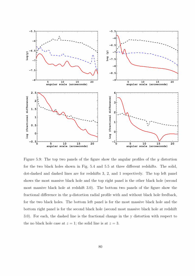
y distortion maps. Section 5.4, will be devoted to describing the scaling relation between y
distortion and black hole mass that has been derived from the simulation. In Section 5.5, I
will compare my numerical results with the analytic results obtained in Chapter 4.
5.1 NUMERICAL SIMULATION
We have used the simulation carried out by Di Matteo et al. (2008). The simulation is an
N-body plus hydrodynamical cosmological simulation that includes radiative gas cooling,
star formation, and for the first time a self-consistent treatment of black hole growth and
feedback. I will briefly discuss the various aspects of this simulation with a special emphasis
on the modeling of black hole growth and feedback.
The numerical code uses a LCDM cosmological model with cosmological parameters from
the first year WMAP results (Spergel et al. 2003). A Gaussian initial condition is used with
a scale invariant primordial power spectrum of spectral index, ns = 1. The normalization
62
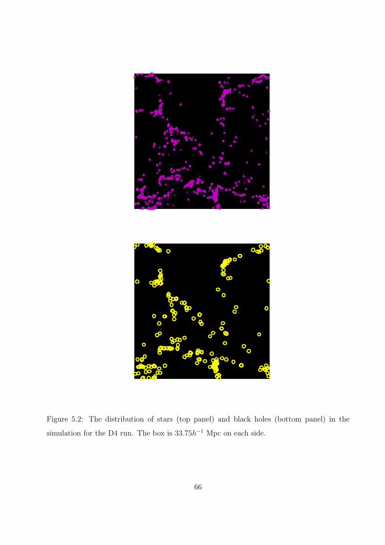
Figure 5.1: The distribution of dark matter (top panel) and gas (bottom panel) in the
simulation at redshift 1.0. The simulation is the D4 run which is the lower resolution version.
We have used this version for our analysis. The filamentary structures are evident from the
map. The gas distribution follows closely the dark matter distribution. The box is 33.75h−1
Mpc on each side.
63
of the power spectrum is done with a σ8 of 0.9. (While a lower value of σ8 will affect the
total number of black holes in a given volume, it should have little impact on the results
for individual black holes presented here.) The simulation uses an extended version of the
parallel cosmological Tree Particle Mesh-Smoothed Particle Hydrodynamics code (TreePM
SPH) GAlaxies with Dark matter and Gas intEracT 2 (GADGET2; Springel 2005). The
Tree PM algorithm is used for carrying out the evolution of the dark matter dynamics and
the Lagrangian SPH method is used to follow gas dynamics. The distribution of dark matter
and gas in the simulation is shown in Fig. 5.1.
5.1.1 N Body Dynamics
The Tree PM (Xu 1995; Bode, Ostriker, & Xu 2000; Springel, Yoshida & White 2001; Bagla
2002) code is a hybrid scheme involving the Tree code (Barnes & Hut 1986) and the Particle
Mesh (PM) (e.g, Efstathiou et al. 1985) code. In a Tree code a hierarchical tree like structure
is obtained for all the particles in a cell like structure unless a cell contains a sub cell or
at least one particle. A cell that is sufficiently far away can be treated as a point source
of mass within the cell and hence the force is computed using a multipole approximation.
Depending on the distance of the cell from the current position, the multipole expansion is
truncated. In a PM code the force is treated as a field quantity. The force is evaluated on a
meshgrid and Fourier techniques are applied on it to calculate the Poisson equation. Both
the PM method and the Tree algorithm have advantages over the direct particle particle
(PP) scheme in terms of time. The main shortcoming of the PM code is that it is resolution
limited (spatial resolution of the mesh) and it is difficult to handle with non uniform particle
distribution. The tree code has the disadvantage of storage space. The hybrid TreePM code
is a combination of both the schemes where a Tree algorithm is used for regions with higher
densities, and a PM approach is used otherwise. This overcomes the limitation of resolution
and storage or time in using the expensive tree code at regions with higher densities and
using the PM code otherwise to save computing time. Other such existing hybrid schemes
are the particle-particle-particleMesh code, (P 3M) (e.g, Couchman 1991), the adaptive mesh
refinement (ART) (Kravtsov, Klypin, & Khokhlov 1997) method etc.
64
5.1.2 Gas Dynamics
Combining dark matter dynamics with gas dynamics (hydrodynamics) has made simulations
more realistic and this allows simulations to link with observations. To do hydrodynamics,
two kinds of approaches are popular. One involves an Eulerian or grid based formalism (Cen
et al. 1990), where the frame of reference is space fixed. The other employs the Lagrangian
description (Smoothed Particle Hydrodynamics (SPH)) (see Monaghan 1992 for a review),
where the frame of reference is body or particle fixed. In a grid based method the gas
properties are defined in a mesh grid whereas in SPH techniques the gas parameters at a
point in the simulation are obtained by averaging the contributions from all the particles
within a smoothing length. New adaptive mesh refinement codes to do hydrodynamics have
been developed by e.g., Truelove et al. (1998); Norman & Bryan (1998). There are relative
advantages and disadvantages for using these schemes to do hydrodynamics. Kang et al.
(1994) and Frenk et al. (1999) does a comparison study of many of the available SPH and
grid codes for cosmological applications. It is now believed that the SPH codes never produce
shocks due to their intrinsic smoothing nature and are generally poorly behaved in low density
regions compared to grid codes (Kang et al. 1994). However for high density regions and
galaxy formation simulations the SPH techniques behave much better since the grid codes
do not tend to conserve angular momentum although the cost of doing SPH simulations is
more than grid codes. In the present simulation SPH is adopted since it involves galaxy
merger simulations.
5.1.3 Supernova and Star-formation
Approximate schemes are employed to model the relevant physics of star formation and the
associated supernova feedback. A hybrid multiphase model for the interstellar medium (ISM)
(Springel & Hernquist 2003) has been used for this case. The modeling of star formation is
described in Appendix E.
65
Figure 5.2: The distribution of stars (top panel) and black holes (bottom panel) in the
simulation for the D4 run. The box is 33.75h−1 Mpc on each side.
66
5.1.4 Black Hole Feedback
A detailed description of the implementation of black hole accretion and the associated
feedback model is given in Di Matteo et al. (2008). Black holes are represented as collisionless
“sink” particles that can grow in mass by accreting gas or by merger events. The Bondi-
V (61) −3090.4± 1305.4 −404.8± 374.4 −656.6± 256.8
W (94) 199.4± 2373.2 −492.2± 670.4 −247.6± 473.4
QF −1973.6± 1274.4 −1018.3± 288.5 −889.2± 259.9
VF −3059.4± 1305.1 −850.6± 340.7 −609.3± 256.7
WF −2249.8± 1503.3 −1072.4± 626.5 −313.7± 47.2
Table 7.8: Effect of the dust mask on the cross-correlation estimator. The amplitude of the
cross-correlation changes significantly once we change the thresholds of our masks.
7.5 INTERPRETATION OF RESULTS
We can now compare our results with theory. We adopt the fits shown in Fig. 7.14 from the
foreground reduced maps for the comparison. We adopt the profile of y distortion described
in Eq. 4.16. We assume the halo mass to be 3× 10¹²M (from the quasar clustering studies
of Coil et al. 2007). We adopt the mean redshift of our sample (z = 1.6) for comparing
with theory. The theoretical values can be obtained from Eq. 5.4. The y distortion fits from
Table 7.6 (3rd and 4th Columns) give y = i0y/i0. This number should be divided by the
pixel size in equivalent steradians (4 × 10⁻⁶). We do not compare our theoretical results
with the other sets shown in Table 7.6, since the fits are not significant. The comparison
between theory and observation is shown in Table 7.9 The values obtained from the data
are two orders of magnitude higher than the values predicted from theory (see Table 7.9).
But we note that the theoretical signal is a strong function of redshift, halo mass, and other
parameters in the model and can vary substantially depending on these parameters. Also,
large scale structures (galaxy clusters for example) are unresolved at WMAP scales and so
116
Fitting Model Observed values of y Theoretical values of y
10−7 10−7
SZ+Dust 5.8± 1.8 .045
SZ 4.2± 2.28 .045
Table 7.9: Comparison between observed and theoretical values of the y parameter. The
theoretical values are obtained from the model described in Chapter 4. Column 1 lists the
models that are used to fit the spectrum.
it is hard to predict the real source of the signal.
WMAP is barely sensitive to the scale of galaxy clusters (e.g; Refregier, Spergel, &
Herbig 2000). The observed correlation of flux decrement with the LRGs is similar to that
for quasars. This suggests that the sources of the signals might be similar. LRGs are tracers
of galaxy clusters and hence the SZ effect that we observe could be originating from galaxy
clusters associated with quasars. Diego & Partridge (2009) finds the SZ signal from galaxy
clusters to be in the range (10− 20) µK (≈ tens of mJy at WMAP frequencies). The fluxes
we get are of the order of 1 mJy. The theoretically predicted SZ signal from quasars is
(10−100) µJy (at WMAP frequencies), depending on the mass of the black hole (Chatterjee
& Kosowsky 2007; Scannapieco, Thacker, & Couchman 2008). Our signal is at least an order
of magnitude higher than the signal that we expect from quasars and an order of magnitude
less than what is expected from massive galaxy clusters. Coil et al. (2007) have studied
the clustering of quasars at redshift 0.7 < z < 1.4 identified by the Deep Extragalactic
Evolutionary Probe 2 Galaxy Redshift (DEEP2) (Davis et al. 2007) Survey and SDSS. The
results show that at these redshifts quasars tend to reside in halos of masses ≈ 3× 10¹²M.
The median redshift of the quasars in our sample is 1.3− 1.4. This implies that the quasars
studied are mostly residing in lower mass halos than galaxy clusters. However if a small
fraction of the total quasars reside in galaxy clusters then that could explain the magnitude
of the signal that we get from our analysis. If 10% of the quasars reside in 1014 − 1015 M
halos we would get a signal of ≈ 1 mJy. This is comparable to what has been observed
117
in the current analysis. The other possibility is that the SZ signal from quasars is higher
(Natarajan & Sigurdsson 1999) than what is obtained from the simulations used to predict
the SZ amplitude.
7.5.1 Projections for ACT
If we assume the size of the source to be 10 arcseconds then the SZ signal in a beam of size θ
(in arcsecond) will be roughly ∆T × (10/θ)2, where ∆T is the theoretical signal described in
Chapters 4 and 5. The beam size for WMAP W band is 12 arcminutes. So for a ∆T of 1 µK
the signal will be 0.2 nK. The noise from WMAP is roughly 30 µK. With 500, 000 sources
this gives a signal-to-noise of .003. Although, by filtering the maps we have increased the
signal-to-noise by a sufficient amount but we are still limited by statistics. It is shown in
Chapter 4 that the signal is a strong function of redshift, halo mass and other parameters.
Within the uncertainties in the modeling parameters, if we assume a theoretical signal to be
about 1 µK, then our estimate shows the signal for ACT to be roughly .03 µK. ACT plans
to attain a nominal noise of 10 µK per pixel. This gives a signal-to-noise of 0.003. Data from
SDSS contain around 30 quasars with photometric redshifts per square degree (Richards et
al. 2006). With a 400 square degrees of sky coverage we can get a 3σ detection of the signal.
However we will still be limited by systematic effects and confusion due to SZ signal from
galaxy clusters.
118
8.0 CONCLUSIONS
In this Chapter, I will summarize the results of this thesis work. In §8.1 I will give the
summary of results. In §8.2 I will describe some of the issues that needs further attention,
and in §8.3 I will suggest some future extensions of this work.
8.1 SUMMARY OF RESULTS
The main goal of this thesis is focused on using the CMB to understand the physics of AGNs.
This involves characterizing the hot gas in AGN environments, via their SZ signatures in the
CMB. Probing black hole energy feedback via SZ distortions gives us a new observational
tool to study the role of AGN feedback in structure formation.
In Chapter 2, I derived the SZ spectral distortion in the CMB from a thermalised distri-
bution of electrons, under the non-relativistic and small energy transfer limit of the Boltz-
mann Equation. This effect was first discovered by Sunyaev & Zeldovich (1969), and the
same results have been reproduced in this thesis. I have also discussed the theoretical and
observational aspects of the CMB with particular emphasis on the SZ effect.
In Chapter 3, I have discussed some theoretical models and observational evidences of
AGN feedback and its role on formation of structures.
In Chapter 4 of this thesis we calculated the SZ distortion from an AGN, using a simple
one-dimensional Sedov-Taylor model of energy outflow. We obtained the profiles of y distor-
tion using simplified assumptions about the source geometry and the redshift distribution
of energy input from the AGNs. The typical temperature of this hot bubble is 106K with
sizes ranging from a few hundred kpcs to a few Mpcs. Using a halo model formalism, we
119
calculated the angular power spectrum of the temperature distortion. The power spectrum
has two peaks. The primary peak occurs at l = 400, which is the correlation scale of large
scale structures. The secondary peak occurs around l = 3×10⁴, at an angular scale of ∼ 20′′
(the characteristic size of a hot bubble at higher redshifts). We investigated the dependence
of the power spectrum on free parameters of the model. Reducing the energy input redshift
zin from 3 to 2.5 reduces the power spectrum by roughly a factor of 2. The dependence on
maximum mass Mmax is relatively weak: the power spectrum amplitude increases only by
60% if the maximum mass is increased by a factor of 5. Using a Gaussian beam we calculated
the signal for a model ACT-like experiment. The signal has an amplitude of the order of
one micro-Kelvin. This signal will be at the noise limit of current arcminute-scale microwave
background experiments, including ACT and SPT.
In Chapter 5, we further characterized the signal from cosmological-hydrodynamical
simulations with black hole feedback. We simulated high resolution maps of the SZ distortion
in the CMB due to the feedback energy from accretion onto supermassive black holes. These
simulations address the rapid accretion phases of black holes (see Hopkins, Narayan, &
Hernquist 2006; Di Matteo et al. 2008). The result is heating of the gas surrounding
the black hole. The results show that with the turn on of AGN feedback the SZ signal gets
enhanced largely and the enhancement is predominant at angular scales of 5 arcseconds. The
signal from the largest black holes has a characteristic amplitude of sub µK to a few µK. We
obtained a scaling relation between the black hole mass and their SZ temperature decrement,
which in turn is a measure of the amount of feedback energy output. We also investigated
the correspondence between y distortion and accretion rates. The correspondence between
the y distortion and the accretion rates is not exact but there is a close association which
shows the correlation between feedback energy output and black hole activity.
In Chapter 6, we designed an experiment using the maps presented in Chapter 5 to
directly detect the signal. The combination of angular scale and small amplitude make
detecting this effect very challenging, at the margins of currently planned experiments. We
show that a very deep observation with ALMA can potentially detect this signal. We also
discuss the technique of detecting this signal by stacking microwave images centered on
known quasars.
120
In Chapter 7, we estimated the cross-correlation signal from the SZ distortion produced
by hot gas in the environments of AGNs by stacking CMB temperature maps from WMAP
centered on SDSS quasars. The effective contamination to this signal comes from dust,
galactic foregrounds, radio emissions from quasars, and the primary temperature fluctuations
in the black body. Different masks and spatial filters are applied to minimize the systematic
effects. We use two models to fit the cross-correlation spectrum. One model involves SZ
and the other model involves SZ and dust. The reduced χ2 values for the two fits are 2.76
and 2.01, respectively. We use the BIC criterion to test the validity of these models. The
BIC values indicate that inclusion of the dust parameter improves the fits significantly. The
best-fit values for the y parameter are (4.2± 2.28)× 10−7 and (5.8± 1.8)× 10−7 respectively,
for the two models. At WMAP scales it is difficult to resolve point sources from galaxy
clusters and so we conclude that the signal is likely to be coming from galaxy clusters.
Finally, we presented the projected signal-to-noise for ACT observations and concluded that
the chances for detecting this cross-correlation signal with ACT is significantly higher than
WMAP within the limits of contamination from other sources.
8.2 DISCUSSION OF RESULTS
The SZ effect from quasars acts as a contamination in SZ surveys that propose to detect
galaxy clusters. Since the amplitude of this signal (∼ 1µK) is well below the amplitude
of the SZ distortion from galaxy clusters (∼ 100µK), this effect will not be important for
detecting galaxy clusters. This signal is at or below the target noise level of SZ experiments
like ACT and SPT. However the signal is interesting, if we consider it as a viable probe for
detecting hot gas in AGN environments. The theoretical models and experimental probes
discussed in this thesis can serve as interesting directions for eventually detecting this signal.
In this Section, I will discuss some of the major issues related to different aspects of the work
described in this dissertation.
The one-dimensional Sedov-Taylor solution is used to model the energetics of the quasar
environment. The Sedov-Taylor model is valid for a point-like explosion in an uniform
121
medium. The assumption of point-like explosion is valid since the duration time of the
explosion is much shorter than the expansion time of the bubble. However the assumption
about the uniform density of the medium needs some justification. The density of the
medium will likely have a power law dependence. In addition, the medium will not be
static (Scannapieco & Oh 2004). The results obtained from numerical models that solve
the coupled differential equations involving radial dependence of the density profile and the
accretion infall are similar to the Sedov-Taylor solution (Barkana & Loeb 2001; Furlanetto
& Loeb 2001). The assumptions of spherical symmetry, uniform temperature, and uniform
density of the gas within the bubble are also approximate. These are used to obtain a closed
form solution. Another assumption involves the redshift distribution of energy injection.
We assume a delta-function distribution where all the quasars eject their energy at a single
redshift. A more realistic approach would use the quasar luminosity functions to characterize
the redshift distribution of quasars.
The other issue involves δs, which relates to the density of the AGN environment. In
simulations AGNs tend to live in dense environments but this needs more observations to
be confirmed. The signal scales weakly with δs. However, depending on the value of δs,
the conclusions about detectibility can vary. Another important issue involves the mode
of energy feedback. As discussed in Chapter 3, the two possible modes of feedback are
radio mode and quasar mode. The radio or the mechanical mode geometry is in the form
of a collimated jet whereas the quasar mode is isotropic. The assumption of isotropy and
spherical symmetry intrinsically implies a quasar mode. Radio loud quasars transport most
of their energy in the mechanical mode. In the radio quiet population the outflow could be
in the form of winds (e.g., Blandford & Payne 1982; Proga, Stone & Kallman 2000; Pereyra,
Hillier, & Turnshek 2006). In both cases the isotropic mode is not the main outflow geometry.
However, the amplitude of the SZ signal will not depend significantly on the mode of energy
transfer.
The next key issue is the assumption about the feedback efficiency. Di Matteo et al.
(2008) assumes that the feedback energy is 0.5% of the rest mass energy when AGNs are
operating in the quasar mode. This assumption is based on the normalization of the M − σrelation. This feedback fraction reproduces the correct M − σ relation in the local universe
122
(Tremaine et al. 2002). Sijacki et al. (2007) investigates AGN feedback in galaxy clusters
with the mechanical mode. The mechanical feedback fraction assumed by Sijacki et al.
(2007) is 2% of the rest mass energy. This assumption predicts an M−σ relation that varies
significantly at the low mass end, from the observed M −σ relation. However the simulation
carried out by Sijacki et al. (2007) reproduces the correct LX − T relation in galaxy groups
and clusters (Puchwein, Sijacki, & Springel 2008). The SZ signal depends on the feedback
efficiency and the assumption on feedback efficiency can also affect the detectibility of the
effect.
The simulation we have used assumes seed black holes, with masses 105h−1M. The
motivation behind choosing a seed mass of 105h−1M comes from currently proposed sce-
narios of seed black hole formation. To have a supermassive black hole of mass 109M in less
than a billion years (as indicated by the z = 6 quasars in SDSS), current theories require,
either: (1) formation of seed black holes of mass 104− 106M from the catastrophic collapse
of supermassive stars (Bromm & Loeb 2003) or (2) formation of smaller seed black holes
(masses 102M) and exponential growth afterwards (Bromm & Larson 2004). The choice
of 105h−1M approximately matches the two scenarios described above. For scenario one,
the choice of seed mass falls in the right range. The seed black holes are introduced into
halos of masses ≥ 1010h−1M. Eddington growth predicts that a black hole of mass 102M
will roughly grow to a value of 105M by the time collapsed objects of masses 1010M are
formed (Di Matteo et al. 2008).
The cross-correlation analysis presented in Chapter 7 shows a first step for detecting the
SZ signal from quasars. At frequencies below the null frequency the SZ signal is a decrement
and this makes it unique compared to the involved systematics at those frequencies. However
observations near and above the null frequency will give more robust confirmation about the
origin of the signal. In the present work we get a deficit in flux which suggests SZ, but the fits
to the observed spectrum are not sufficiently robust to confirm this conclusion. It is possible
that these results come from the cold spots in the primary CMB signal but the primary CMB
signal is unlikely to correlate with quasar positions. We need further investigations to study
the source of this signal. Wright et al. (2009), Hinshaw et al. (2007), and Chen & Wright
(2008) report detections of negative fluxes associated with the point source amplitudes in
123
the WMAP 3yr and 5yr point source catalogs. The observed correlation with the LRGs are
the same as the observed correlations with quasars. This suggests that the source of the
signal might be similar. LRGs are tracers of galaxy clusters and hence the SZ effect that we
observe can also be originating from galaxy clusters. We note that the detection of the SZ
effect from quasars will always suffer from the systematic noise of SZ distortion from galaxy
clusters.
The optimum way to disentangle the cluster contribution is to look at field AGNs. Also
the SZ effect is still sub dominant at angular scales probed by WMAP (see Komatsu &
Seljak 2002). The Planck surveyor satellite and ongoing CMB experiments like ACT and
SPT will be sensitive to scales where the SZ signal will be more dominant compared to the
primary temperature fluctuations. This will increase the signal per pixel from SZ. Resolving
galaxy clusters in Planck or ACT maps will give us a better control on subtracting the cluster
contribution to the SZ signal. The detector noise thresholds for Planck and ACT/SPT will
be an order of magnitude lower than WMAP. This makes the plausibility of detecting this
signal better with future CMB experiments. The filtering technique that has been used
in the current work has certain limitations in dealing with CCMBl as a noise term. Chen &
Wright (2008) introduce a CMB free filtering technique which increased the number of source
detections in the 5yr maps. This technique can also be applied to the current problem.
8.3 FUTURE WORK
There can be several possible extensions of the work presented in this thesis.
The mass scaling relations shown in Table 5.3 capture the time-dependent component
of AGN feedback. The simulation that we have used offers the possibility of tracking the
accretion history and duty cycle of an individual black hole. The issue of time dependence
of feedback and its connection with accretion rates can be studied by simulating the SZ
signal and observing its time dependence over the whole evolutionary history of a black hole.
The simulation also offers the possibility of studying quasar environments and how they
depend on different parameters. One of the interesting application would involve studying
124
Figure 8.1: Co-added maps of the AGNs (in the EGS field) in three X-ray bands. The three
bands are 0.5 − 2 Kev (left), 2 − 4 Kev (middle), and 4 − 7 Kev (right). The maps are 5
arcminutes on each side.
the environmental effects on accretion rates of supermassive black holes from the simulation.
Prochaska & Hennawi (2008) show a novel technique to study the environments of a quasar
by using a background quasar in the line of sight to study the physical state of the foreground
quasar. With KECK HIRES Echelle spectograph they measured HI column densities. The
measurement of these column densities will provide constraints on the kinematics, tempera-
ture and ionization structure of the quasar environment (Prochaska & Hennawi 2008). Our
simulations can be used to compute HI column densities around individual black holes. The
results from the simulation can be directly compared with the data.
With the simulation we can also do an X-ray analysis of the black hole environments
which will be complimentary to the SZ analysis that we have already done. With a combined
X-ray and SZ analysis of the same effect we will be able to put stronger constraints on the-
oretical models of feedback. The X-ray results can be directly compared with observations.
Currently, I am involved in detecting AGN feedback (Chatterjee et al. 2009 (in prep)) by
stacking Chandra maps of DEEP 2 AGNs in the Extended Groth Strip (EGS). The stacked
X-ray maps are shown in Fig. 8.1 in three energy bands. An interesting application of the
cross-correlation analysis will involve stacking galaxy clusters from public X-ray and Optical
125
catalogs (SDSS-MaxBcg) to detect the SZ signal from galaxy clusters. ALMA mock obser-
vations derived from the simulations and the maps presented in Chapter 5 will be useful in
outlining the feasibility of direct detection.
The CMB has been used as a back light to study a number of physical processes in the
universe. In the present work we emphasize the technique of using the CMB to study an
important aspect of theories involving galaxy formation, namely feedback from AGNs. I
hope this work will initiate more exciting and detailed studies in the field.