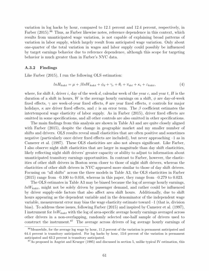
No. 18-2

The Supply Side of Discrimination: Evidence from the Labor Supply of Boston Taxi Drivers

Osborne Jackson Abstract This paper investigates supply-side discrimination in the labor market for Boston taxi drivers. Using data on millions of trips from 2010–2015, I explore whether the labor supply behavior of taxi drivers differs by the gender, racial/ethnic, or age composition of Boston neighborhoods. I find that disparities in shift hours due to neighborhood demographics exist even when differences in local earnings opportunities are taken into account. I observe heterogeneity in the amount that drivers discriminate and find that this discrimination is primarily statistical rather than taste-based. As drivers gain experience and learn to better anticipate wage variation, discrimination decreases. Keywords: discrimination, labor supply, Boston taxis, wage elasticity JEL Classifications: J71, J22, J31, L91

Osborne Jackson is a senior economist with the New England Public Policy Center, located in the research department at the Federal Reserve Bank of Boston. His e-mail address is osborne.jackson@bos.frb.org. The author thanks an anonymous vendor for providing data on taxi trips in Boston, as well as Chris Foote, Bob Triest, Albert Saiz, seminar participants at the 2018 American Economic Association Annual Meeting, the 2018 Society of Labor Economists Annual Meeting, the Federal Reserve Bank of Boston, Ohio State University, Rensselaer Polytechnic Institute, and Tufts University, and anonymous referees for their helpful comments. Outstanding research assistance was provided by Kevin Behan and Thu Tran. This paper presents preliminary analysis and results intended to stimulate discussion and critical comment. The views expressed herein are those of the author and do not indicate concurrence by the Federal Reserve Bank of Boston, or by the principals of the Board of Governors, or the Federal Reserve System. This paper, which may be revised, is available on the web site of the Federal Reserve Bank of Boston at http://www.bostonfed.org/economic/wp/index.htm.

This version: January, 2019; original version posted in June, 2018

1 Introduction

Researchers have devoted much attention to understanding discrimination against legally

protected classes across a variety of markets. Focusing on the labor market, economic theories

and evidence regarding discrimination largely center on the market’s demand side (Altonji

and Blank 1999; Cain 1986). However, discrimination can also occur on the supply side

of the labor market.1 Such supply-side discrimination could be taste-based (that is, due

to personal prejudice), especially if workers have some degree of market power, or it could

be statistical if workers have incomplete information about the potential buyers of their

labor. This discriminatory behavior is thus important to understand, particularly in light of

nontrivial numbers of part-time, self-employed, and “gig” economy workers who may have a

greater opportunity to engage in such actions given market structures.

Using evidence from the Boston taxicab industry, this paper investigates the extent of

supply-side labor market discrimination and its mechanisms. The taxi industry has often

served as a useful setting for economists to study labor supply behavior, largely due to

the flexible hours that cab drivers have, unlike many other professions. Existing work has

focused on whether taxi drivers dynamically respond to higher wages by working more hours,

behavior that is consistent with neoclassical labor supply theory, or by working fewer hours,

a choice consistent with income targeting and a behavioral model with reference-dependent

preferences (for example, Camerer et al. 1997; Crawford and Meng 2011; Farber 2005, 2015).

Building on the work of Farber (2015), who finds evidence of upward-sloping intertemporal

labor supply, this paper examines whether the willingness of cab drivers to supply labor at

a given wage differs based on the demographic composition of the areas in which they work.

I utilize data on millions of trips from taxi drivers in Boston over a six-year period from

1For instance, an area of discussion in Colorado and Oregon was the legality of individuals refusingto work on the basis of their religious beliefs to provide wedding cakes for same-sex couples (see Ameri-can Civil Liberties Union of Colorado, “Court Rules Bakery Illegally Discriminated Against Gay Couple,”from ACLU website: http://aclu-co.org/court-rules-bakery-illegally-discriminated-against-gay-couple, andsee Todd Starnes, “Oregon Silences Bakers Who Refused to Make Cake for Gay Wedding,” from Fox Newswebsite: http://www.foxnews.com/opinion/2015/07/06/state-silences-bakers-who-refused-to-bake-cake-for-lesbians.html).

1

2010–2015 to test for the presence of supply-side labor market discrimination. I observe that

disparities exist in the supply of taxi services across Boston neighborhoods with different

demographics, even when market differences in largely unanticipated local earnings oppor-

tunities are taken into account. These conditional disparities in shift hours across areas are

evidenced by wage elasticities that vary by neighborhood composition. Specifically, wage

elasticities are 5 to 7 percent lower as the population share of female, black, or Asian resi-

dents at trip pick-up locations rises by 1 percentage point (that is, 2 to 11 percent of the area

share sample mean, depending on the demographic group). The presence of such supply-side

discrimination in a driver’s willingness to work longer is robust to several analysis checks,

including relaxing sample restrictions, incorporating tips into local wages, adding a proxy for

local costs, and assessing the role of trip drop-off locations compared to pick-up locations.

I also find heterogeneity across cab drivers and areas in the amount of estimated discrim-

ination. Using a decomposition of this variation in discrimination estimates as well as other

empirical tests, I try to determine the underlying mechanism for the observed behavior. I

find evidence that the drivers’ choices are primarily caused by statistical rather than taste-

based discrimination, and that as drivers gain experience and learn how to better anticipate

wage variation in areas, they engage in less discriminatory behavior. These results suggest

that although supply-side labor market discrimination may occur under certain market con-

ditions, it need not persist. Moreover, policies supplying earnings-relevant information to

workers about those purchasing their labor might speed up the rate of learning, thereby mit-

igating discrimination. Lastly, the paper’s findings also suggest that individuals can learn

to optimize across both time and space, although perhaps at different rates. The findings

are also supported by alternative, trip-level estimation I conduct that exploits the quasi-

experimental exposure to neighborhoods of different demographic compositions that drivers

experience based on trip drop-off locations, conditional on a given trip pick-up location.

Among existing studies, some evidence has been found of disparities in taxi services across

Boston neighborhoods, although these disparities are not attributable solely to differences

2

in driver labor supply due to the absence of controls for market wages and other variables

(Austin and Zegras 2012; Nelson\Nygaard Consulting Associates 2013). In a study of the

taxi industry in New York City (NYC), Haggag, McManus, and Paci (2017) examine how cab

drivers engage in on-the-job learning, including the accumulation of neighborhood-specific

experience, in order to improve their ability to find customers and increase earnings per shift.

However, they do not examine whether differences in driver behavior across neighborhoods

are potentially attributable to discrimination. Examining ridesharing rather than taxis,

Ge et al. (2016) conduct an audit study in Boston and Seattle to test whether drivers of

companies such as Uber and Lyft discriminate among customers. Ge et al. (2016) find a

pattern of discrimination, as evidenced by longer wait times for black passengers in Seattle,

and in Boston, a higher rate of trip cancellations for black passengers and longer, more

expensive rides for female passengers. My paper contributes to the existing literatures on

both disparities in ride transportation and intertemporal labor supply. It is a study that

incorporates market wages to determine the extent of discrimination in the labor supply

choices of cab drivers across neighborhoods with different demographics.

The remainder of the paper is organized as follows: section 2 provides background on the

taxi industry in Boston and discusses the data used on taxi trips. Section 3 examines how

these trips vary across locations. Section 4 outlines models of area-specific labor supply with

discrimination, while section 5 presents the main findings regarding the existence of such

discrimination. Section 6 determines the presence of driver and area heterogeneity regarding

discriminatory behavior, while section 7 explores whether supply-side discrimination is taste-

based or statistical. Section 8 discusses alternative, quasi-experimental estimation, and

finally, section 9 concludes.

3

2 Background and Data on Boston Taxi Drivers

Taxicabs in Boston, historically called “Hackney Carriages,” are licensed by the Police Com-

missioner under the authority of Chapter 392 of the Acts of 1930 and have been regulated

by the Hackney Carriage Unit of the Police Department since the unit’s founding in 1854.2

There are 1,825 taxi medallions in Boston, with an upper limit on the number of cabs set

by the City of Boston.3 A Boston taxi medallion owner usually falls into one of the fol-

lowing categories: 1) buys or leases a vehicle, affixes the medallion, and “shifts” out the

medallioned taxicab to drivers (48 percent of the 1,825 taxis); 2) buys or leases a vehicle,

affixes the medallion, and operates the vehicle him/herself as an owner-operator (25 percent

of the 1,825 taxis); 3) leases the medallion to a vehicle owner, who affixes the medallion

and operates the taxi (20 percent of the 1,825 taxis); or 4) hires someone to manage his/her

medallions, either by “shifting” out a medallioned taxicab or leasing the medallion to a

vehicle owner (5 percent of the 1,825 taxis) (Nelson\Nygaard Consulting Associates 2013).

Thus, Boston cab drivers fall into one of three main categories: owner-operators (453

persons in 2013), leased medallion drivers (number unknown), or shift drivers who rent a

medallioned taxicab over a weekly or 12-hour period (number unknown but likely the major-

ity of drivers given that this is how most medallions are used) (Nelson\Nygaard Consulting

Associates 2013). Drivers are free to work as few or as many hours as desired within any shift

constraint, if applicable.4 Meanwhile, in terms of expenses and earnings, drivers pay for any

leasing or shift fees plus fuel and a handful of other potential authorized charges, while they

2See Boston Police Department, “Hackney Carriage Unit,” from BPD News website:http://bpdnews.com/hackney-carriage-unit/. The most recent major revision to these regula-tions, Rule 403, became effective August 29, 2008 (see City of Boston, “Boston Police Depart-ment Rule 403 Hackney Carriage Rules and Flat Rate Handbook,” from City of Boston website:http://www.cityofboston.gov/tridionimages/rules tcm1-3045.pdf).

3New York City, with 13,238 medallions, has 7.3 times more taxi licenses than Boston (Farber 2015).However, this disparity is smaller when considering the number of medallions issued per square mile, whichis 43.5 for NYC and 20.4 for Boston, or the medallions issued per 1,000 persons which, according to 2015American Community Survey population estimates, is three in Boston versus two in NYC (Minnesota Pop-ulation Center 2010).

4Cab fleets (“radio associations”) may place constraints on the timing and duration of shifts for theirdrivers. By City regulation unless exempt, all medallion owners must affiliate with a radio association whichprimarily dispatches trips requested by customers (Nelson\Nygaard Consulting Associates 2013).

4

keep all fare income plus tips.5 Because of this industry structure, as Farber (2015) argues,

“the driver internalizes the costs and benefits of working in a way that is largely consistent

with an economist’s first-best solution to the agency problem with risk-neutral agents.”

In terms of locations, pick-ups are authorized within the driver’s licensed jurisdiction

(that is, Boston’s city limits), but drop-offs may occur outside of Boston if requested by the

passenger. Within Boston, drivers are not restricted regarding where they travel or whom

they pick up, whether as street hails or trips offered through the dispatch system, which they

can freely accept, decline, or not respond to (Nelson\Nygaard Consulting Associates 2013).

However, by regulation, drivers “may not refuse any passenger on the basis of race, sex,

religion, disability, sexual orientation, national origin, or location of the passenger’s pick-up

or destination in any circumstance.”6 Thus, discrimination may be manifested by certain

groups encountering longer wait times when hailing or requesting a taxi, or drivers being less

likely to service areas where members of those groups tend to reside.7 This paper examines

the latter mechanism.

Taxi drivers only earn income when they have a passenger in the cab and the meter is

running. Over the 2009–2015 period covered by my data, income in the “meter zone” is

earned at the rate of $2.60 for the first one-seventh of a mile (the “drop rate”) plus either

$0.40 for every additional one-seventh of a mile (the “mileage rate”) or $28 per hour when

the cab is not moving (the “waiting time rate”). Outside the “meter zone,” which applies

to trips from Boston to suburban cities and towns beyond a 20-mile radius from Boston,

income is earned according to flat rates as published in the Official Flat Rate Handbook.8

5Authorized charges may include optional additional insurance, fees for failing to return a shifted vehicleon time, tolls from Boston proper to Logan International Airport, and so on.

6See City of Boston, “Boston Police Department Rule 403 Hackney Carriage Rules and Flat Rate Hand-book,” from City of Boston website: http://www.cityofboston.gov/tridionimages/rules tcm1-3045.pdf. Oneexception to this anti-discrimination rule is that a driver may refuse a passenger if there is justifiable fearfor the driver’s safety or if the passenger is incapacitated.

7See Elisabeth Bumiller, “Cabbies Who Bypass Blacks Will Lose Cars, Giuliani Says,” from NewYork Times website: http://www.nytimes.com/1999/11/11/nyregion/cabbies-who-bypass-blacks-will-lose-cars-giuliani-says.html, and see Eric Roper and Alejandra Matos, “Taxicab Drivers Skirting MinneapolisLaws,” from Star Tribune website: http://www.startribune.com/june-29-taxi-drivers-skirting-minneapolis-laws/265066351.

8See City of Boston, “Boston Police Department Rule 403 Hackney Carriage Rules and Flat Rate Hand-

5

There are also discount coupons available for Boston residents 65 years of age and older and

for disabled residents of all ages which cab drivers are required to honor.9

As of 2009, the City of Boston required all taxis to be equipped with electronic devices

that allow for credit card processing of payments.10 For all trips (not just those paid by

credit card), these devices record information on various trip details including the fare, the

trip start and end times, and the trip start and end locations via global positioning system

(GPS) capabilities. The City of Boston has access to these data for planning and regulatory

purposes, with two vendors supplying devices for all but a handful of cabs (Nelson\Nygaard

Consulting Associates 2013).

I have obtained data from one of these two major vendors on taxi trips taken in the

“greater Boston market” from April 2009 to January 2016, which I further restrict to the

period running from May 1, 2009 to December 31, 2015, to better ensure complete data for

all months.11 These data identify drivers by encrypted Hackney Carriage license number and

medallions (cabs) by encrypted medallion number.12 My Boston data sample is smaller than

book,” from City of Boston website: http://www.cityofboston.gov/tridionimages/rules tcm1-3045.pdf.9See Boston Police Department, “Hackney Carriage Unit,” from BPD News website:

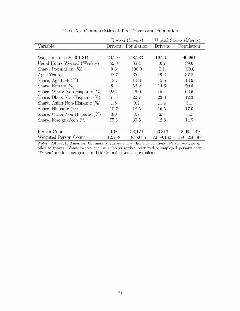
http://bpdnews.com/hackney-carriage-unit/. In terms of net earnings after costs, a recent 2013 con-sulting report estimates that the annual pre-tax net earnings of a full-time Boston taxi driver rangesfrom $51,910 to $65,675 depending on the medallion ownership category, while a part-time shift driver isestimated to earn $35,883 (Nelson\Nygaard Consulting Associates 2013). However, 2010–2015 AmericanCommunity Survey data on Boston taxi drivers and chauffeurs in Table A2 (pooling across six years in orderto draw a larger sample of employed persons) lists earnings for this group during that period at $20,298 in2010 dollars (Minnesota Population Center 2010).

10When first announced, this change was slated to become effective January 1, 2009 (seeCity of Boston, “Boston Police Department Rule 403 Hackney Carriage Rules and Flat RateHandbook,” from City of Boston website: http://www.cityofboston.gov/tridionimages/rules tcm1-3045.pdf). However, the change ultimately became effective later in the year (seeEric Moskowitz, “Credit Card Use Frustrates Cabdrivers,” from Boston.com website:http://archive.boston.com/news/local/massachusetts/articles/2011/05/16/credit card use frustrates cabdrivers).

11The “greater Boston market” largely represents data from licensed City of Boston taxicab fleets, whichis why I focus here on regulations from the City of Boston. However, the “greater Boston market” alsoreflects data from other fleets in close vicinity (for example, Cambridge). Trips from such out-of-town fleetscould start or end in Boston, albeit, illegally in the former case.

12When restricting the data to trips that start in Boston proper, and after correcting for some medallionnumbers in the data with missing leading zeros, I observe 1,313 unique medallions. It is reassuring thatthis value is well below the 1,825 medallions issued in Boston, especially since trip data is missing from thesecond major vendor of credit card processing devices. Additionally, some subset of these 1,313 medallionslikely reflects cabs not licensed in Boston that are conducting illegal pick-ups in Boston. Citations by theBoston Police Department for illegal pick-ups grew from 305 in 2011 to 513 through the first two-thirds of2013, with drivers and medallion owners suggesting that the illegal pick-up problem is even more prevalent

6

the NYC sample used by Farber (2015), in part because Boston is a smaller market and also

due to the absence of data from the second major device vendor. In my data, on average

there are about 7.5 million trips taken annually in taxicabs in the Boston area. About 8,100

drivers earned at least one fare in a cab over the nearly seven-year period, with roughly 3,800

drivers appearing in the data during a single year. Approximately 800 drivers worked in all

of the sample years, and the median driver is observed in the data for three calendar years.

While I use as much of the available data as possible, much of my analysis is based on a

random one-half sample of the drivers (see Appendix and section 3 for further details).

In terms of data limitations, similar to Farber (2015), I cannot identify which medallions

are associated with particular shift drivers, leasing drivers, or owner-operators. Because

these three categories of drivers face different constraints and incentives relevant to their

labor supply choices, it would be ideal to analyze their behavior separately. However, out

of necessity, I group all types of drivers together.13 Also, like Farber (2015), I do not

have complete information on tip receipts. Thus, I exclude tips from fare totals (other

than sensitivity analysis in section 5) and assume that tipping rates are not correlated with

average hourly fare earnings.14

3 Variation in Trips and Demographics Across Boston

To begin the spatial analysis of taxi trips in Boston, for a given driver, I define a gap between

trips of six hours or more as indicating the end of one shift and the start of another (see

Appendix for details). I start with a sample of 26,602,914 trips that underlie a one-half sam-

ple of 1,788,470 shifts and 4,052 drivers used in non-spatial analysis performed to replicate

Farber (2015) (see Appendix). I then impose a few additional sample restrictions, both in

the estimation one-half sample as well as the non-overlapping one-half sample of 27,179,101

than the citation numbers suggest (Nelson\Nygaard Consulting Associates 2013).13One possibility might be to assume that unique medallion-driver pairings are (a subset of) owner-drivers

and focus some analysis on this subgroup. However, there are very few such drivers in my data (for example,in Table 1, only 18 drivers, or less than 1 percent, fall in this category).

14See Haggag and Paci (2014) for an examination of tipping behavior in NYC cabs.

7

trips associated with 1,820,251 shifts and 4,076 drivers. Specifically, across all 3,608,721

of the aforementioned shifts and 53,782,015 associated trips, observations are dropped for

which a shift:

1. contains any trip without start location information (1,577,407 shifts and 22,275,790

associated trips; 41.4 percent of 53,782,015 trips);

2. contains any trip that does not start in Massachusetts (9,170 shifts and 165,373 asso-

ciated trips; 0.3 percent of 53,782,015 trips);

3. starts in 2009, given that the baseline data on demographics from the U.S. Census

is from 2010, as discussed below (184,021 shifts and 2,741,607 associated trips; 5.1

percent of 53,782,015 trips).

I restrict the sample at the shift level, not at the trip level, so that each shift (non-

spatial) contains its full set of trips and area-specific shifts, thus not inducing bias given

estimation at the area shift level. Because I’m analyzing driver behavior, I focus on the

start locations of trips; compared to end locations, this is the spatial component over which

drivers have more control. These restrictions result in a final spatial sample of 28,599,245

trips associated with 1,838,123 non-spatial shifts and 6,896 drivers. For the analysis, I rely

on a random one-half sample of 3,435 drivers with 912,679 non-spatial shifts comprised of

14,136,226 trips.15 In this final spatial estimation sample, 13,643,800 of the total 14,136,226

trips start in Boston proper (96.5 percent), leaving 492,426 trips (3.5 percent) starting in

other parts of the greater Boston area or elsewhere in Massachusetts.

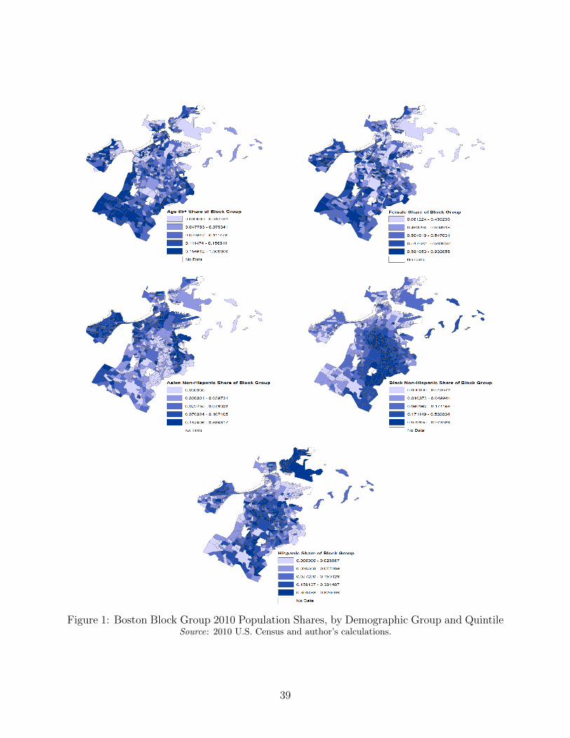
Regarding resident demographics, Figure 1 maps the area population shares across the

558 Boston block groups in the 2010 U.S. Census that are female, black non-Hispanic, Asian

non-Hispanic, Hispanic, and 65 years of age and older (Minnesota Population Center 2010).16

15The final spatial non-overlapping sample contains 3,461 drivers with 925,444 non-spatial shifts comprisedof 14,463,019 trips.

16While the full data includes areas outside of Boston proper, for visual ease, I restrict the maps to Boston.In contrast to all area residents, I also examine 2010–2015 American Community Survey data on Boston taxidrivers and chauffeurs in Table A2 (pooling across six years in order to draw a larger sample). This group of

8

For each of the five demographic (or “minority”) groups depicted, there is variation across

Boston in the local population share of the group.17 Still, some spatial clustering exists.

For instance, the Boston neighborhoods of Roxbury, Dorchester, and Mattapan tend to have

some of the highest shares of black residents in the city. Meanwhile, near Logan International

Airport, the East Boston neighborhood has a high concentration of Hispanic residents, while

Allston, Brighton, and Chinatown are among the neighborhoods with the highest shares

of Asian residents.18 There is a less discernible pattern with the distribution of women or

individuals who are 65 years of age and older, although Hyde Park and West Roxbury seem

to have notable concentrations of these two groups.19

Turning to the taxi data, across all 52,584 clock hours in the data from January 1, 2010

to December 31, 2015, I calculate area averages for the number of trips and hourly earnings.

The realization of these variables in the raw data represents drivers’ labor supply as well as

residents’ labor demand. For a given hour × area pairing in the trip-level data, I determine

the number of trips taken and total trip earnings for each driver with at least one trip in

the hour × area. I then take the average of each of those variables across the given drivers

within the hour × area, followed by taking the average once again across all 52,584 clock

hours in the data. This calculation results in averages of driver hourly trips and driver hourly

earnings for each area during the sample period.

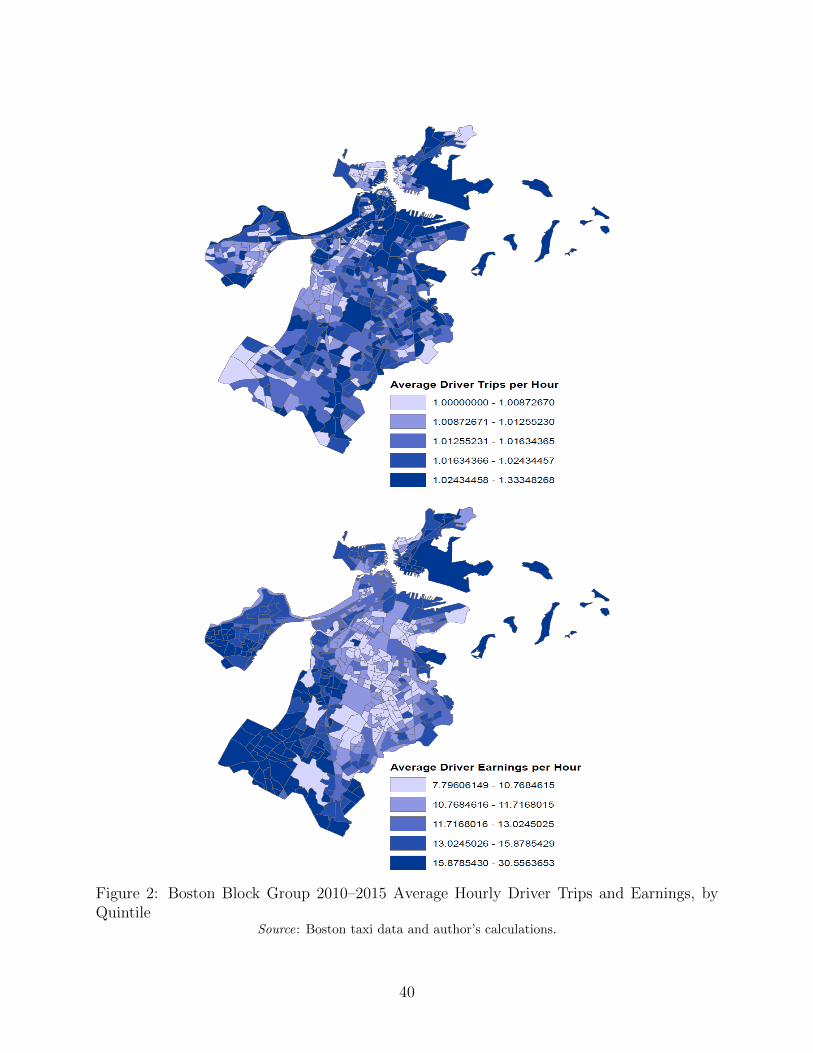
Figure 2 shows the average driver trips per hour and hourly earnings from 2010 to 2015

for taxi trips taken in Boston areas categorized as 2010 U.S. Census block groups, focusing on

the trips’ starting locations.20 Although not purged of demand-side influences and averaged

drivers, representing 12,258 persons (weighted, or 0.31 percent of the total Boston population; 108 personsunweighted), is 8.4 percent female, 61.5 percent black non-Hispanic, 1.8 percent Asian non-Hispanic, 10.7percent Hispanic, 12.5 percent 65 years of age and older, as well as 75.6 percent foreign-born (MinnesotaPopulation Center 2010).

17In the main estimation sample to be discussed, area population shares for all five groups average lessthan 50 percent, thus allowing the minority group description used here to be accurate.

18There are 133 block groups comprising quintile 1 for which the share of Asian residents is zero, rangingfrom a minimum overall population of 10 residents to a maximum overall population of 2,461 residents.

19The maximum share of residents 65 years of age and older equals 1 due to a six-person block group inHyde Park.

20I also examine this figure using trip end locations. As expected, since drivers presumably have lesscontrol over end locations than start locations, the variation across block groups in trips per hour is more

9

over time, the spatial variation in the upper map of Figure 2 nevertheless gives some insight

into how labor supply choices (on the intensive margin) by drivers might differ across areas.

Conditional on working in a block group, drivers tend to work in that block group about once

per hour, and up to 1.33 times per hour. Meanwhile, the lower map of Figure 2 examines

spatial variation in average driver earnings per hour. Although not purged of supply-side

influences and averaged over time, to the extent that the map captures labor demand-driven

hourly earnings, it shows that there is substantial variation in such wages across areas. Per

block group, average hourly wages range from $7.80 to $30.56, with values in the median

block groups spanning $11.72 to $13.02.

In later regression analysis of cab driver labor supply, the goal will be to examine to what

extent wage elasticity differences across areas are attributable to labor supply discrimination.

This estimation will allow me to address shortcomings of the previous descriptive analysis

by purging the influence of labor demand and non-discriminatory labor supply, and also by

conditioning on the local earnings opportunities facing drivers. Such analysis will use the

current intermediate dataset of 14,136,226 trips associated with 912,679 non-spatial shifts

from a random one-half sample of 3,435 drivers, from which a final dataset of area shifts

will be constructed for spatial regression analysis. But before proceeding to estimation, it is

helpful to first consider the theoretical underpinnings of the analysis.

4 Models of Labor Supply with Discrimination

4.1 Taste-Based Discrimination

In the spirit of Becker (1957), I can model labor supply-side discrimination as due to animus.

The key features distinguishing this model from a statistical discrimination framework are a

wage rate that is certain and a group distaste parameter in the utility function.

The setup and results of this model are detailed in the Appendix, so I focus here on im-

compressed, with a maximum value of 1.14 for the end location map instead of 1.33 in Figure 2.

10

plications and testable predictions. The model shows that differentials in gross log area work

hours by cab drivers, when area wages are not included as a regressor in the estimation, need

not reflect taste-based discrimination. The theory also predicts that discrimination yields

slope differences in labor supply across areas with high and low shares of minorities, not just

intercept differences. Non-discriminatory, driver-specific tastes may generate compensating

wage differentials and thus also need to be controlled for, either using driver fixed effects (if

driver tastes don’t differ across areas) or else alternatives (if driver tastes do differ across

areas, or if it is preferable to exclude driver fixed effects). The model assumes that wages

across areas are demand-driven, so empirically, this assumption requires imposing various

controls for driver labor supply and using instrumental variables (IV) estimation in order

to isolate the wage variation due to demand. The theory also suggests that controlling for

driver fixed effects should diminish but not completely eliminate taste-based discrimination,

as there is a distribution of distaste parameters across areas for a given driver. However,

driver × area fixed effects should eliminate this form of discrimination.

Additionally, because the choice to engage in discrimination means drivers forgo some

earnings, any increased competition that affects market wages will alter drivers’ allocation

of hours across areas. The model shows that if competition in low minority areas increases

sufficiently more than in high minority areas, this will drive down wages in low minority areas

enough compared to high minority areas to cause drivers to increase the hours supplied to

high minority areas.

4.2 Statistical Discrimination

Alternatively, in the spirit of Phelps (1972) and Aigner and Cain (1977), I can model supply-

side discrimination in the labor market as due to incomplete information about earnings

opportunities. The key features distinguishing this model from a taste-based discrimination

framework are a wage rate that is uncertain and the absence of any group-specific distaste.

Once again, the Appendix describes the detailed model setup and results, while this

11

discussion focuses on testable predictions and implications. Similar to before, the model

shows that when area wages are not included as a regressor in estimation, differences in gross

log area work hours by cab drivers need not reflect statistical discrimination. The theory also

predicts again that discrimination yields slope differences in labor supply across areas with

high and low shares of minorities, not just intercept differences. Moreover, including controls

for anticipated wage variation should not affect the amount of statistical discrimination

since this behavior is driven by unanticipated wage variation. Also, the model shows that

controlling for driver fixed effects should diminish but not completely eliminate this form of

discrimination, given different anticipated wage means by minority share.

The theory also predicts that with increases in the “reliability ratio” — a measure of

the proportion of local wage variation anticipated by a driver — differences in log hours and

expected log hours across places with different minority shares will decrease. In other words,

statistical discrimination is mitigated as the reliability ratio increases, since anticipated wages

correspond more closely to realized wages. Following Farber and Gibbons (1996) and Altonji

and Pierret (2001), if the reliability ratio approaches one over time because drivers gain

more experience and are better able to increase the share of realized wage variation that is

anticipated, then this form of discrimination should diminish over time. Accordingly, driver

× area fixed effects should not eliminate this form of discrimination given such variation

with driver experience.

5 Shift-Level Estimates of Supply-Side Discrimination

5.1 Estimation Strategy

I now turn to econometric estimation of differences across areas in the slope of taxi driver

labor supply, and the extent to which such differences vary by the demographic composition

of areas.21 To do so, I need to rely on exogenous labor demand shifts within areas while hold-

21I cannot credibly identify differences across areas in labor supply intercepts (see Appendix).

12

ing driver labor supply in each area constant. As Figure 3 shows, due to potential demand

differences across areas that might cause false conclusions about area-specific driver supply,

the identifying demand variation must be within locations rather than across locations. To

identify driver labor supply slope differences across locations (via elasticity differences), the

changes in (inverse) demand causing wage changes are assumed to be identical across areas

(that is, ∆Dj = D′j − Dj = ∆Dk ∀j 6= k areas, D,D′).22 Estimating differences across

areas in labor supply elasticities solely from within-area variation can thus address demand

or non-discriminatory supply differences across areas that are time-invariant.

To examine whether area demographic composition causes differential responses of cab

driver area shift hours to area wage increases, I estimate the following equation:

lnHkidcta = µ+ βlnWkidcta + (lnWkidcta ×Ma)′η + φd + γc + θt + πdct + αa + εkidcta. (1)

In equation (1), for shift k, driver i, day of the week d, calendar week of the year c, year

t, and area a, H is the area-specific duration of a shift in hours, M is a vector of “minor-

ity”/demographic population shares (that is, black, Asian, Hispanic, female, and 65 years

of age and older, all as measured in the 2010 Census), W is the area-specific average hourly

earnings on a shift, and ε is an error term, with standard errors clustered at the driver

level.23 Also, φ controls for day-of-week fixed effects, γ controls for week-of-year fixed ef-

fects, θ controls for year fixed effects, α controls for area fixed effects, and π controls for

major holidays.24 Similar to Farber (2015), these additional controls help to satisfy iden-

22This assumption would hold, for instance, if conditional on controls, changes in demand were randomshocks. This further highlights that identifying differences in labor supply elasticities across areas will beeasier than identifying intercept differences across areas if, conditional on controls, changes in demand havea greater stochastic component than levels of demand.

23While the demographic shares in M could alternatively be allowed to vary over time using AmericanCommunity Survey data, there is likely little variation in many of these shares from 2010 to 2015. Also,focusing on 2010 Census data allows block group composition to be based on a much larger underlyingsample. Meanwhile, the choice of 65 years as the age threshold is partly motivated by the qualifying ageof the Taxi Discount Coupon Program, which reduces the cost of cabs to the elderly via coupons andmay provide motivation for cab drivers to avoid such passengers (See Boston Police Department, “HackneyCarriage Unit,” from BPD News website: http://bpdnews.com/hackney-carriage-unit).

24As in Farber (2015), major holidays are defined as New Year’s Day, Easter Sunday, Memorial Day,Fourth of July, Labor Day, Thanksgiving, and Christmas Day.

13

tification assumptions by accounting for some anticipated variation in wages. Such wage

variation likely contributes to driver labor supply differences within areas, as well as differ-

ences across areas in passenger demand and non-discriminatory driver supply. If supply-side

discrimination based on area demographics exists, I expect wage elasticity parameters η < 0,

reflecting diminished wage sensitivity of work hours as the minority share increases.

Since demand or non-discriminatory supply may vary over time, I can also replace fixed

effects φd, γc, θt, and αa with φdt, γct, and αat.25 Driver fixed effects, κi, or driver × area

fixed effects, κia, may also be added to further account for supply differences within areas

or non-discriminatory supply differences across areas. If such fixed effects are not actually

needed for consistent estimation of discrimination parameters, then they might instead help

to inform the mechanism likely generating discrimination, as discussed in the theory.

5.2 Constructing Area-Specific Shift Hours and Wages

In order to estimate equation (1), I need to define hours, H, and wages, W , so that they

are area-specific variables. Regarding hours, within each shift, I assign an area to a taxi trip

based on the trip’s starting location. The duration of an area-specific “stint” is defined as

the duration of the trip plus the duration of the driver’s wait time until the start of the next

trip in the shift, if applicable. The area-specific shift duration, Hkidcta, is the sum of all of

these trip stints within a given area a. The total shift duration then generally equals the sum

across locations of the area-specific shift durations, or Hkidct =∑

aHkidcta.26 If drivers have

more control over wait time than trip duration, then area shift duration captures a driver’s

willingness to wait for a subsequent trip (that is, willingness to work longer searching for the

next fare) given a current trip that starts in area a.27

25Given the large number of fixed effects to estimate, to improve computational speed I rely on the Statacommand reghdfe, which implements an estimator described in Correia (2016). As a check, for more basicspecifications with fewer fixed effects, I compare reghdfe with least-squares dummy variable estimation(with and without instrumental variables) and obtain identical estimates, standard errors, and statistics.

26Because I truncate both area-specific and non-area-specific shifts longer than 24 hours to be equal to 24hours (see Appendix), Hkidct =

∑aHkidcta may not hold in these infrequent truncated shift cases.

27Unfortunately, I do not observe continuous information on areas traversed by a driver during trips andwait times to incorporate in the construction of area hours and wages.

14

Area-specific average hourly earnings, Wkidcta, are defined as the total earnings from all

trips that originate in area a within a non-spatial shift, divided by the area-specific shift

duration, or Wkidcta = Ekidcta/Hkidcta, where Ekidcta is area-specific total earnings. This wage

has the reasonable feature that for a given earnings amount in an area, the wage decreases

either as the area trip length increases or as the wait time until the next trip increases.

Thus, starting from an intermediate dataset with a random one-half sample of 3,435 drivers

associated with 912,679 non-spatial shifts, this formulation of area hours and wages results

in the creation of 9,890,638 area shifts.28

Sometimes, the average hourly earnings of an area-specific shift are quite high and may

result from measurement error. In order to retain much of the sample while still removing

erroneous shifts, I implement a threshold for area-specific average hourly earnings of $25.

This threshold value is guided by theory (see Appendix), and I will also explore the sensitivity

of the analysis to this sample restriction. Once imposed, along with a few other sample

restrictions, I obtain a dataset of 3,744,057 area-specific shifts from 2,984 drivers.29 Average

values of the demographic shares in the sample of dropped shifts do not differ substantively

from their values in the retained sample.30 Across shifts in the retained sample, area shift

duration is 0.86 hours at the median and 1.25 hours on average, while average hourly area

earnings are $15.78 at the median and $15.21 on average. Also, the number of trips per

area shift is 1 at the median and 1.56 on average, while the number of trips per shift in the

non-spatial analysis is 14 at the median and 14.87 on average (see Appendix).

28The non-overlapping sample contains 10,116,926 area shifts from 3,461 drivers.29This estimation sample drops observations where the area shift hours or area wages are zero, since both

are in log form for estimation. The sample also ensures a constant number of observations across all variationsof equation (1) and Appendix equation (3), thus conditioning on non-missing regressors (including Xa) inall cases. Lastly, the sample additionally imposes that the instrument for IV estimation, to be discussed, isnot missing. A non-overlapping sample that applies the same restrictions as the estimation sample contains4,094,076 area-specific shifts from 2,973 drivers. However, the relevant non-overlapping sample, which onlyconditions on area wages being non-zero and no greater than $25—that is, the appropriate conditions forinstrument construction, the non-overlapping sample’s sole purpose—contains 4,476,441 area-specific shiftsfrom 3,406 drivers.

30For instance, the difference across samples in the average Asian share is 0.04 percentage points, or 0.3percent of the retained sample mean Asian share (13 percent).

15

5.3 Main Results

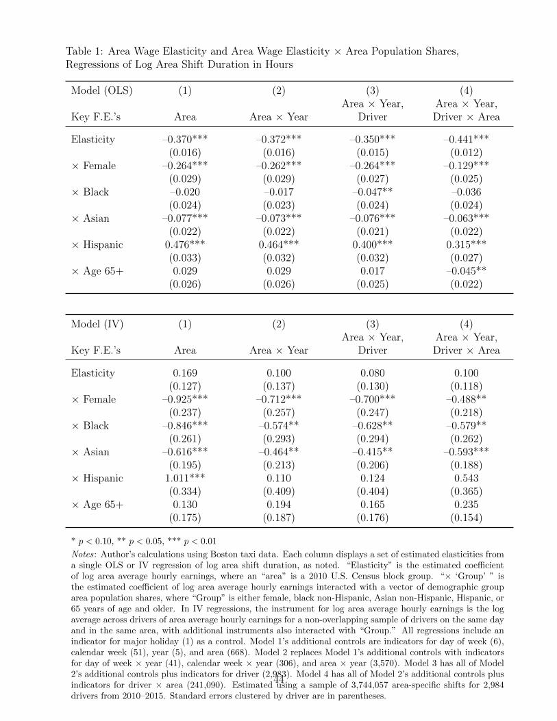
The upper panel of Table 1 presents OLS estimates from equation (1) of area wage elasticity

β and the vector of discrimination parameters η from interactions of the area wage with

area population shares.31 Given inclusion of the interaction terms, the “baseline” elastic-

ity β should be interpreted as the average area wage elasticity for a block group with a

demographic composition of only male residents below 65 years of age, none of whom are

black, Asian, or Hispanic. OLS results across all specifications display significantly negative

baseline area wage elasticities while estimates of discrimination, when significant, are also

generally negative.

These OLS estimates may be biased, however, because the log of area-specific average

hourly earnings, lnWkidcta, might not be solely driven by passenger demand, and rather could

be influenced by driver supply-side factors that also affect area shift hours. Additionally, due

to shift hours appearing as the dependent variable and in the denominator of the independent

wage variable, measurement error may bias the wage elasticity estimate toward –1 (that is,

division bias). To address these issues, following Farber (2015) and in the spirit of Camerer

et al. (1997) (see Appendix), I instrument for lnWkidcta with the average across other drivers

of log area-specific average hourly earnings. As Farber (2015) proposes, to avoid problems

arising from using an instrument derived from the dependent variable in estimation, I use the

non-overlapping, randomly selected one-half subset of drivers to construct the instrument.32

The average across drivers of log average hourly earnings of shifts k on day of week d,

calendar week c, year t, and in area a (lnW kdcta) in the non-overlapping sample serves as the

31There are also significant gross disparities in area shift hours by local demographic composition. Froman OLS regression of log area shift duration on a vector of area population shares, with 3,744,057 area shiftsfor 2,984 drivers from 2010–2015, the coefficients are all significant at the 1 percent level: –0.513 (female),–0.227 (black), –0.280 (Asian), 0.763 (Hispanic), and 0.182 (65 years of age and older). However, theseassociations may simply reflect area-specific differences in earnings opportunities rather than discriminationby drivers.

32As proposed in Angrist and Krueger (1995), unlike typical IV estimation, this split-sample IV estimationis biased toward zero rather than the probability limit of the OLS estimate. Thus, in the presence of biasedestimation, using split-sample IV estimation results in wage elasticities that offer a more neutral stancebetween neoclassical and behavioral models of labor supply, rather than biased support for the latter.

16

instrument for the log of average hourly earnings for driver i with shifts k that start on day

of week d, calendar week c, year t, and in area a (lnWkidcta) in the estimation sample.33 This

instrument should capture demand-driven movements in the log wage that are not affected

by supply-side driver choices or measurement error, thus purging from estimation any driver

supply differences within areas.

The bottom panel of Table 1 presents IV estimates from equation (1). Parameter es-

timates are similar across specifications, although coefficient magnitudes differ. I focus on

the three specifications with area × year fixed effects as the preferred, more conservative

estimates. The baseline area wage elasticity β̂ is positive across these specifications, albeit

not significant, ranging from 0.08 to 0.10. These coefficients are in line with microeconomet-

ric estimates of the non-spatial Frisch labor supply elasticity, which tend to range from 0

to 0.5 (Altonji 1986; MaCurdy 1981; Peterman 2016), including this paper’s own estimates

ranging from 0.37 to 0.48 (see Appendix). This provides some reassurance that the area

wage is reasonably constructed.34

IV estimates of the discrimination terms, η̂, indicate how the baseline wage elasticity β̂

differs as the demographic composition of area residents changes. These η̂ terms are signifi-

cantly negative for the female, black, and Asian shares, and are positive but not significant

for the Hispanic and aged 65 years and older shares in preferred specifications.35 For in-

33While I do not present first stage results, they are very strong. In a basic version of model (1) from Table1 with the interaction terms omitted, the first stage F-statistic is 462. The coefficient on the instrumentis 0.034, notably smaller than in the non-spatial analysis where the instrument coefficient is close to 1 (seeAppendix). This indicates a weaker relationship between the wages other drivers face on a given shift anda driver’s own wages faced on the same shift when that comparison is restricted to a given block group.Meanwhile, when considering the full equation (1) with six endogenous regressors, the Stock and Yogo(2005) weak instrument identification critical values for the maximal actual size of a 5 percent Wald testof the six wage instruments jointly being equal to zero are 29.18, 16.23, and 11.72 for maximal test sizesof 10, 15, and 20 percent, respectively. The joint F-statistic on the six instruments always far exceeds thefirst critical value when estimated separately for each of six endogenous wage regressors in all but one case,where it still exceeds the second critical value.

34Although drivers are not very responsive to the baseline area wage, spatial labor supply responsivenessmay be greater in other cases, such as when considering the extensive margin. The intensive margin spatialanalysis in this paper aligns with the non-spatial analysis in the Appendix, Farber (2015), and other mi-croeconometric analyses of the Frisch labor supply elasticity that focus on the intensive margin response ofhours to wage increases, conditional on working at least some hours.

35The Hispanic share coefficients become negative but not significant when the East Boston region, whereLogan Airport is located, is dropped from the sample, with estimates ranging from –0.31 to –0.64.

17

stance, as the Asian share in a block group increases by 1 percentage point in specification

(2), the baseline wage elasticity 0.100 declines by 0.0046, or 4.6 percent. If the Asian pop-

ulation share were to increase from 0 to 0.13, the mean value in the estimation sample, the

baseline wage elasticity would decline by 0.06, or 60 percent, resulting in a wage elasticity

of 0.04. Thus, in response to a 10 percent increase in the area wage, hours worked in the

area increase by only 0.4 percent rather than 1 percent due to greater Asian representation.

Given a mean area wage in the sample of $15.21 and a mean area shift of 1.25 hours, on

average, a $1.52 increase in the local wage leads to an increase of 0.0125 hours worked in a

baseline area (45 seconds) compared to an increase of 0.005 hours worked (18 seconds) in an

area with the mean Asian population share, a disparity of 27 seconds. When this area labor

supply difference for a given driver is aggregated across all drivers in a day, the disparity

can become notably larger. For the 2,189 calendar days in the sample, there are on average

401 drivers on a given day.36 Thus, across 401 drivers, given a 10 percent increase in the

area wage, the average disparity in area shift length is three hours, equivalent to 2.4 area

shifts and 3.75 trips (given 1.56 trips per area shift, on average). This corresponds to at

least four fewer passengers served on a given day due to local demographics in a block group

with average Asian representation. Moreover, this effect size becomes larger when considered

across multiple areas, days, and demographic groups.

Likewise, increases of 1 percentage point in the female or black population shares lower

the baseline wage elasticity by 0.0071 (7.1 percent) or 0.0057 (5.7 percent), respectively, in

specification (2). Including driver fixed effects in specification (3) does not have much effect

on the β̂ or η̂ estimates. Model (3) has more modest identification assumptions but may

eliminate some supply-side discrimination if models (2) and (3) are both identified. Lastly,

if models (3) and (4) are both identified, given the inclusion of driver × area fixed effects in

model (4), coefficient similarity across models suggests that the primary mechanism behind

driver behavior may be statistical discrimination rather than taste-based discrimination.

36While there are 2,191 calendar days from January 1, 2010 to December 31, 2015, January 31, 2010 andMarch 14, 2010 do not appear in the final estimation sample and are dropped.

18

With 1 percentage point increases in the female, black, or Asian shares, the baseline wage

elasticity now decreases by 4.9 to 5.9 percent. The η̂ female coefficient differs the most

across specifications (3) and (4), perhaps indicating that taste-based discrimination plays the

largest role for this demographic group. To the extent that animus is driven by demographic

differences between those who discriminate and their targets, Table A2 further supports the

possibility of taste-based discrimination toward women. Among the five demographic groups

in η̂, the largest population share disparity between Boston drivers and all residents exists

for women (44 percentage points). Additional analysis in sections 6 and 7 will help further

explore the relevant mechanism(s) underlying observed discrimination.

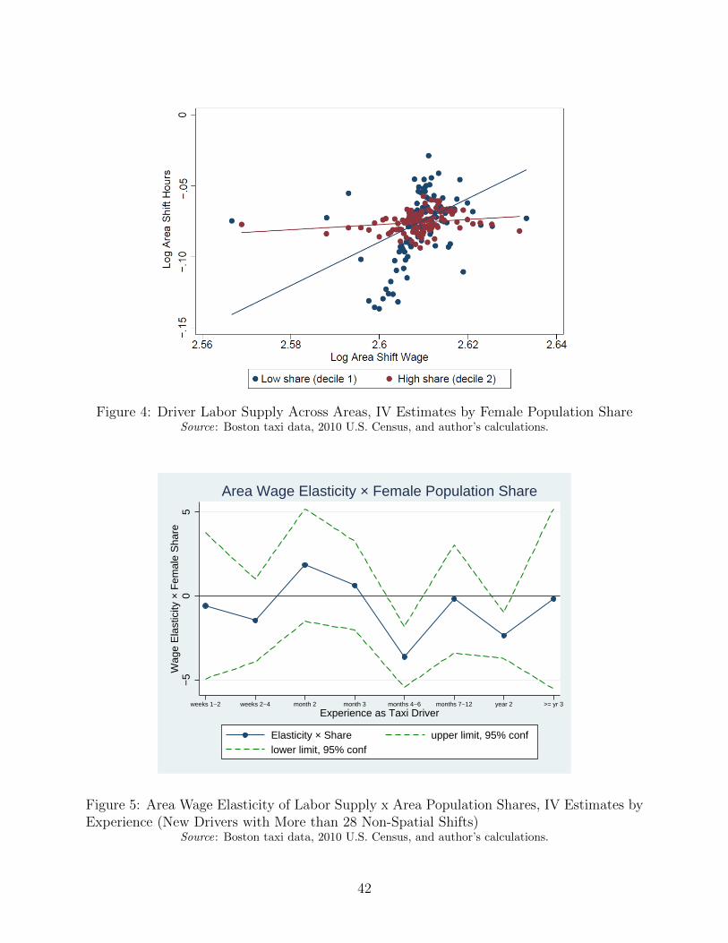
A binned scatterplot in Figure 4 provides a nonparametric view of the impact of dis-

crimination on driver labor supply, analogous to IV estimation in Table 1.37 To represent

marginal effects of η̂ that correspond to continuous changes in the area female population

share, I plot supply curves for first and second decile female representation. Aligned with

Table 1 regressions and the upper plot of Figure 3 (axes transposed), Figure 4 shows that

labor supply is less wage sensitive when the female population share is larger.

5.4 Robustness Checks

Given that the regressor of interest in equation (1) is lnWkidcta ×Ma, I might worry about

bias related to either (or both) the log area wage or area demographic share components of

that term. Table 2 displays analyses testing the robustness of the discrimination findings,

concentrating on analogs of specification (4) from Table 1.

Focusing first on lnWkidcta, if tips in addition to fares also significantly affect driver

labor supply and are correlated with area demographic shares and log area wages, then

discrimination due to fare-based wages may be absent once wages based on fares plus tips

are considered. Models (1) and (2) of Table 2 show that whether considering all shifts or

37Absent an IV estimation routine in Stata’s binscatter command, I plot log area shift hours on fittedvalues of the log area shift wage (from a first stage regression), controlling for the indicators in Table 1 model(2) and five interaction terms of the observed log area shift wage and demographic shares.

19

only shifts where at least one trip is paid for by credit card (since tip information is only

available for taxi fares paid for by credit card), evidence of discrimination still remains when

wages incorporate tips. Also, baseline elasticity estimates (now significant) remain positive

and in the expected range.38

Turning to Ma, if some other area variable observable to drivers is correlated with area

demographic shares and log area wages, then estimated discrimination may be spurious,

capturing wage sensitivity to the omitted variable. Criminal activity is a candidate for such

an omitted variable, but 2010 crime rates at the block group level are not readily available.

Instead, in model (3) of Table 2, I examine educational attainment as measured in the 2006–

2010 five-year American Community Survey (Minnesota Population Center 2010), as it is

potentially relevant for explaining non-discriminatory driver labor supply.39 While education

is not observable to drivers and thus is not an ideal candidate variable, it may nevertheless

be correlated with observable area amenities that drivers might care about, such as safety

or infrastructure quality.40 In model (3), there remains evidence of discrimination and a

reasonable baseline wage elasticity, although there is also now a significantly positive result

(10 percent level) for the age 65 years and older share.41

The remaining models of Table 2 now consider lnWkidcta ×Ma in its entirety. Models

(4) and (5) show that addressing potential bias from omitted time-of-day driven demand

(either AM/PM or hourly) still results in sensible baseline wage elasticities and estimated

discrimination. Model (6) considers that omitting area costs per hour and their interaction

38Some cash trips in the raw data have non-zero tip information due to measurement error and are adjustedto equal zero.

39Specifically, I examine the share of the area population 25 years of age and older whose educationalattainment is a high school diploma.

40Alternatively, I attempted to include interactions between the log wage and 32 region fixed effects inorder to explore non-discriminatory factors affecting driver labor supply elasticities (see Appendix for regiondefinitions). However, I was unable to precisely estimate any of the elasticity coefficients with this approach.

41It is unclear how much weight to place on this specification. Since educational attainment is not directlyobservable to drivers, it is uncertain which neighborhood amenities, if any, attainment is correlated with thatwould affect driver labor supply. Consistent with this ambiguity, when the share of those with a high schooldiploma is replaced with the share of those with some college, I obtain an unexpected and highly negativecoefficient on the interaction of the wage elasticity with the college share, as compared to the positive (butnot significant) coefficient for the share of those with a high school diploma.

20

with area population shares may bias discrimination estimates if hourly earnings and hourly

costs are correlated. I use the log of average area hourly trip distance as a proxy for fuel costs,

since fuel expenditures will depend multiplicatively on distance traveled, vehicle miles per

gallon, and the price of a fuel gallon. With area costs included, estimate precision is reduced

since the model now tries to separately identify benefit and cost elasticities, which are both

non-linearly related to distance. Thus, larger coefficient magnitudes should be given less

weight, although the significantly positive baseline wage elasticity is still in line with macro

and some micro estimates of the non-spatial Frisch elasticity. Interestingly, the baseline

cost elasticity is of equal but opposite magnitude, revealing symmetric driver labor supply

responses to benefits and costs. Evidence of wage-related discrimination is still observed,

and similarly, drivers are less cost sensitive toward female and Asian demographics.42

Additionally, I examine the sensitivity of the results to focusing on area shifts at or

below the $25 area wage threshold imposed due to measurement error considerations. First,

as noted, I observe no economically significant difference between average area demographic

shares in the sample with area wages at most $25 and the sample with area wages above

$25. Model (7) nevertheless displays results for an expanded, combined sample of area

shifts. While I still observe evidence of discrimination (although now with a significantly

positive coefficient for the age 65 and older share as well), the baseline wage elasticity is now

significantly negative. Sample stratification at $25 reveals that this is due to negative but

imprecise wage elasticity estimates for the sample with area wages above $25. Put differently,

there is a “bend” in area labor supply that the linear model masks, resulting in a substantive

difference in discrimination parameters across the sample. That is, discrimination with a

positive baseline wage elasticity reflects decreased neoclassical behavior, while discrimination

with a negative baseline wage elasticity reflects increased income targeting behavior. Thus,

this paper’s results can be interpreted as focusing on the former, reflecting driver behavior

for a range of area wages where the area labor supply curve is upward-sloping, and where

42Considering area costs via distance also helps to address one mechanism through which trip drop-offlocations could matter.

21

area wages are more likely to be free of measurement error. Meanwhile, increased income

targeting behavior can still be interpreted as a form of discrimination since, given an area

wage increase, drivers are more willing to reduce work hours in high-minority areas than

low-minority areas, thereby contributing to greater area disparities in access to taxi services.

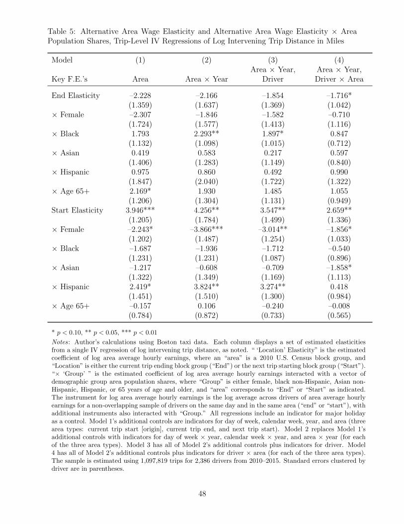
Lastly, given the focus of the analysis on trip pick-up locations, I also consider the role

of drop-off locations. Examining how demographics correlate between pick-up and drop-

off locations reveals that there tends to be only a mild, positive relationship between start

and end location residential composition. Thus, observed discrimination based on trip start

locations is unlikely to be conflating discrimination based on trip end locations.43

6 Discrimination Variation By Driver and Area

Having estimated average labor supply discrimination, I now examine variation in these

discrimination estimates by driver and area. I take advantage of the large sample of 3,744,057

area-specific taxi shifts to explore this heterogeneity. Focusing on one demographic group at

a time and stratifying by driver-region-experience cells, I want to decompose how much of

the variation in discrimination occurs: (a) within driver-areas, (b) across areas for a given

driver, and (c) across drivers but area-invariant, where (b) and (c) combined account for

variation between driver-areas.44 The more variation in discrimination that exists within

the driver-area dimension, the greater the credence that such discrimination is statistical

rather than taste-based. This reasoning follows directly from the theory outlined in section

4 and the Appendix, where only statistical discrimination may vary within the driver-area

dimension due to driver learning over time, whereas variation between driver-areas could be

due to statistical or taste-based discrimination.

43However, even if so, estimated coefficients would still reflect unbiased estimates of location-based dis-crimination, even if not unbiased estimates of start-location discrimination specifically.

44Regions are large Boston neighborhoods or Massachusetts counties, rather than block groups, to ensurea sufficient number of block group shifts for estimation. Driver experience “periods” occur every six weeks,where a week is seven non-spatial shifts (and one to six shifts are rounded up to a week). Further detailsare in the Appendix.

22

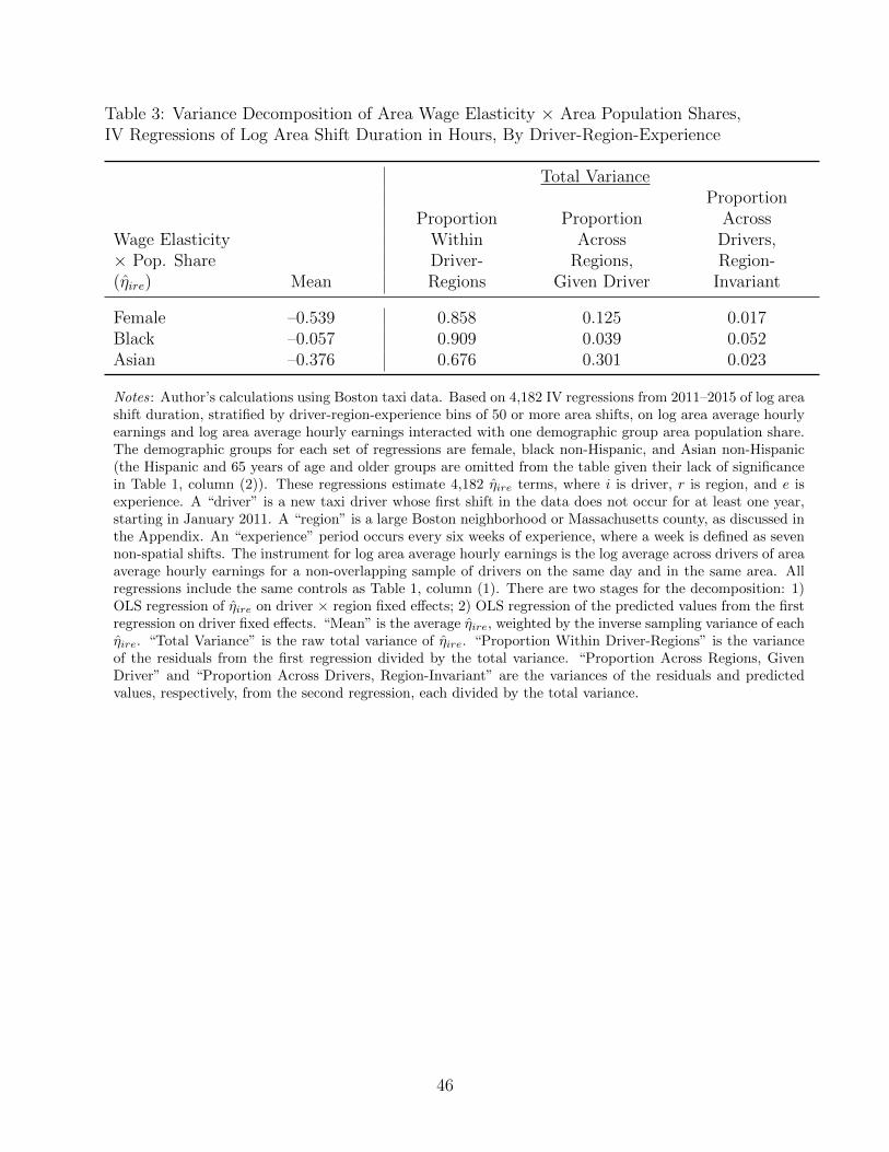
Table 3 displays the results from the variance decomposition. For each demographic

group, the mean wage elasticity-population share interaction across driver-region-experience

(ire) cells is negative for all three demographic shares. Each mean lies within a confidence

interval of 95 percent (female, Asian) or 99 percent (black) of the IV estimates from model

(4) of Table 1, despite specification differences (for instance, examining one demographic

group at a time here for η̂ire). Meanwhile, regarding the decomposition of total variance, the

majority of the variation for all three sets of η̂ire estimates occurs as experience varies within

driver-regions: with 85.8 percent for the female share, 90.9 percent for the black share, and

67.6 percent for the Asian share. This finding suggests that it is possible that the majority

of labor supply discrimination by taxi drivers is statistical.

The remaining variation in the η̂ire estimates occurs across driver-regions and is experience-

invariant, thus providing scope for taste-based and/or statistical discrimination. Variation

across regions for a given driver can be thought of as discrimination taking place on the

“intensive margin,” as it depends on a demographic group’s concentration in an area. This

margin accounts for 12.5 percent of η̂ire variation for the female share, 3.9 percent for the

black share, and 30.1 percent for the Asian share. Meanwhile, the variance proportion across

drivers that is region-invariant can be thought of as “extensive margin” discrimination, as

it does not depend on the concentration of a demographic group in an area. This margin

represents 1.7 percent of η̂ire variation for the female share, 5.2 percent for the black share,

and 2.3 percent for the Asian share.

7 Do Drivers Discriminate for Different Reasons?

7.1 Taste-Based Discrimination

To further explore the potential role of driver preferences and taste-based discrimination in

my findings, I begin by examining how the discrimination term η varies with driver experi-

ence in Figure 5, now stratifying the estimation sample by experience bins only, rather than

23

also by driver and region.45 As discussed in section 4 and the Appendix, if the discrimi-

nation estimated in this paper is taste-based, I would expect η to be relatively constant as

driver experience increases, since tastes are assumed to be time-invariant.46 However, if dis-

crimination is statistical, then I might expect η to approach zero as drivers gain experience

and learn to better anticipate area-specific wage variation, thereby placing less weight on

neighborhood demographics to assess wages.

Focusing on estimates for the female demographic group, Figure 5 shows that the wage

elasticity-population share interaction term generally remains negative as driver experience

increases (plots for the black and Asian shares, not shown, are similar).47 This largely

time-invariant pattern would seemingly be consistent with taste-based discrimination. How-

ever, due to wide confidence intervals, I cannot rule out the possibility that drivers may

initially discriminate but that this discrimination diminishes and approaches zero as experi-

ence increases, consistent with statistical discrimination. It is only in the case of the female

population share specifically that I observe somewhat stronger evidence in favor of taste-

based discrimination, as η is significantly below zero in months 4–6 and year two, fairly

late in a driver’s experience cycle. The possibility that discrimination against women may

be driven by both taste-based and statistical mechanisms is consistent with the results pre-

sented in Table 1, where inclusion of driver × area fixed effects in specification (4) reduces

the magnitude of η by the most for the female group.48

45Rather than six-week experience bins, the experience period lengths now match those in Farber (2015)and follow the non-spatial analysis in Appendix Figure A11, except for the aggregation of weeks 1–2 andweeks 3–4 in order to obtain more reasonably precise estimates.

46As noted in the Appendix, while discrimination preferences might change over time for some individuals,it seems plausible to assume that they are stable for Boston cab drivers given the older age of this population(see Table A2).

47Figure 5 reflects IV estimation of specification (1) from Table 1. Given fewer observations obtainedfrom restricting the sample to new drivers, especially within an experience category, specification (1) is morefeasible to estimate with some precision than specification (2). However, because experience categories oftenfall within a calendar year, estimating specification (1) in Figure 5 should closely approximate estimatingspecification (2) in Table 1. Although Figure 5 restricts the sample to 1,000 new drivers with more than28 non-spatial shifts (that is, approximately four weeks of experience), analogous figures for a sample of allnew drivers look nearly identical, suggesting that driver exit is not particularly related to estimates of laborsupply discrimination.

48Following the theory set forth in section 4 and the Appendix, I also examine the influence of in-creased market competition from ridesharing companies on discriminatory behavior and industry exit by

24

7.2 Statistical Discrimination

To further explore the potential role of statistical discrimination in my findings, one test I can

run, guided by the theory in section 4 and the Appendix, is to examine whether the amount

of estimated discrimination varies with a proxy for the reliability ratio, ψ.49 The reliability

ratio, which ranges from 0 to 1, reflects the share of total wage variation that is anticipated,

and thus somewhat captures a driver’s degree of wage certainty. To generate the ratio, I run

an OLS regression of lnWkidcta on indicators for day of week, calendar week, year, area, and

major holiday. The predicted values from this regression capture anticipated log area average

hourly earnings, ̂AlnW dcta, while the residuals from this regression capture unanticipated

log area average hourly earnings, ̂UlnW kidcta. The numerator of the reliability ratio is the

sample variance across days and weeks of anticipated log area average hourly earnings by

area-year, V̂ ar(AlnW )at. The denominator of the reliability ratio is the sum of the sample

variance of anticipated log area average hourly earnings by area-year, V̂ ar(AlnW )at, and

the sample variance across shifts, days, and weeks of unanticipated log area average hourly

earnings by driver-area-year, V̂ ar(UlnW )iat. Thus, I generate the reliability ratio proxy,

ψ̂iat = V̂ ar(AlnW )at

V̂ ar(AlnW )at + V̂ ar(UlnW )iat, which I calculate in each year in order to allow the ratio to

cab drivers. I utilize entry into the Boston market by Uber on October 24, 2011 (see Scott Kirsner,“Test-riding Uber, the Populist Car Service You Summon with a Mobile App,” from Boston.com web-site: http://boston.com/business/technology/innoeco/2011/10/test-riding uber the populist.html), Side-Car on March 15, 2013 (see Janelle Nanos, “SideCar Launches in Boston,” from Boston Magazine web-site: http://www.bostonmagazine.com/news/blog/2013/03/15/sidecar-launches-in-boston/), and Lyft onJune 1, 2013 (see Michael Farrell, “Lyft is Latest Ride-Sharing App to Offer Service in Boston,” fromBoston Globe website: https://www.bostonglobe.com/business/2013/05/31/car-sharing-app-lyft-arrives-boston/g2fi9ixj707RU9MSXKWQ8O/story.html), limiting the sample to shifts undertaken by new drivers(that is, no shifts in 2010) who are “active” with at least one shift from January 1, 2011 to October 23,2011 before the entry of ridesharing firms. Once again, I observe no evidence of driver exit due to marketcompetition that is correlated with η values. However, this result may be partly due to the identificationof ridesharing competition effects solely from entry dates of ridesharing firms, given the lack of accessiblespatial data on ridesharing trips.

49Section 4 and the Appendix also show that statistical discrimination results solely from unanticipatedwage variation, not predicted wage variation. This finding suggests that if including controls for predictedwage variation reduces the magnitude of the discrimination parameter estimates, at least some of the dis-crimination is taste-based. However, this test cannot be performed because, as discussed in section 5, thesecontrols are necessary for valid identification of parameters. Alternatively, one could examine deviationsfrom wage expectations within area × day × hour bins, to see if driver behavior varies in bins with moreuncertainty. However, unlike the reliability ratio, such an approach would not allow wage uncertainty to becaused in part by drivers, as the theory in the Appendix suggests.

25

vary roughly by driver experience.50

I estimate equation (1) with IV, as in Table 1, but now add a regressor for the reliability

ratio proxy as well as the interaction of the ratio with lnWkidcta ×Ma.51 According to the

model (see Appendix), if the underlying mechanism for discrimination is statistical, then

the coefficients from the interaction of the reliability ratio with the relevant log area wage ×

demographic share regressors will be positive. In other words, as the reliability of anticipated

wage variation increases, statistical discrimination should be reduced.

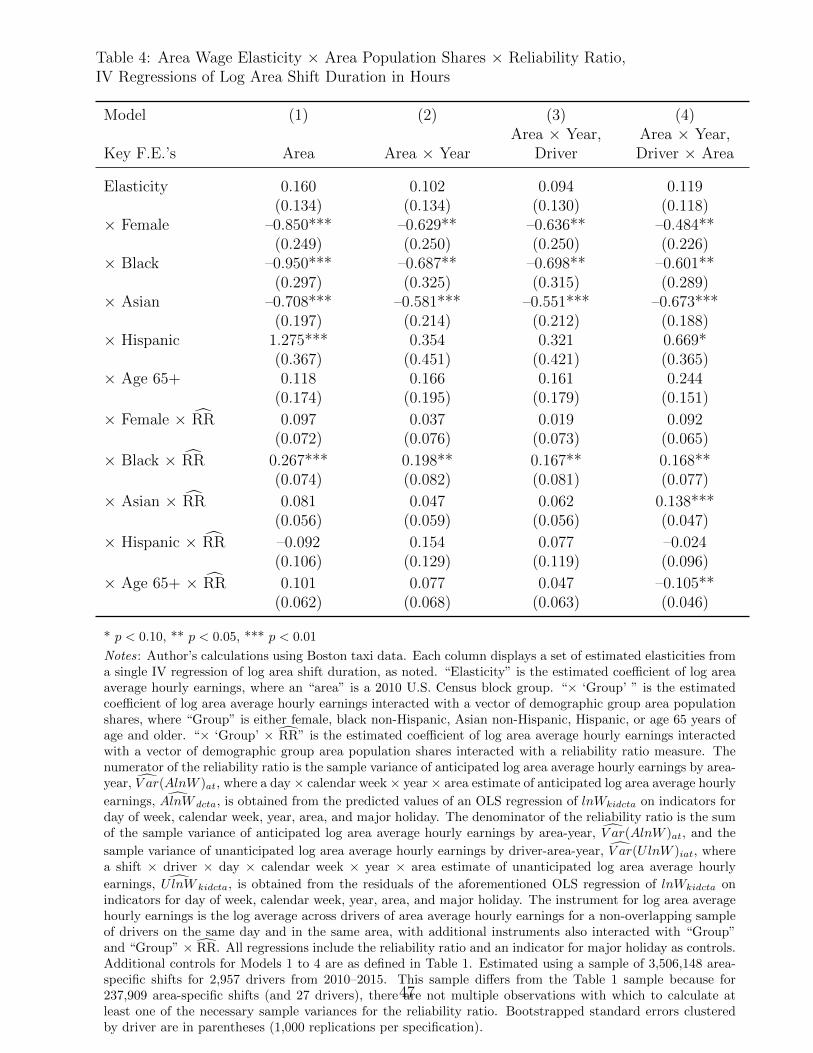
Table 4 presents IV estimates of how discrimination varies with the reliability ratio proxy.

The ratio itself has a mean of 0.02 in the estimation sample, with a standard deviation of

0.07, a minimum very close to 0 (1.4× 10−6), and a maximum of 1. Baseline wage elasticity

estimates, β̂, and interactions with demographic shares, η̂, are very similar to results in

Table 1, although interpretation across tables differs since Table 1 estimates correspond to a

reliability ratio of zero. I focus on specification (4) which isolates variation that is more likely

specific to statistical discrimination. For instance, as the reliability ratio increases by 0.01,

the negative effect of 0.0060 on the baseline wage elasticity from a 1 percentage point increase

in the black share is reduced by 0.0017, or about 28 percent. I likewise observe a significantly

positive effect on the Asian population share η. Across specifications, these results suggest

that a reliability ratio in the 0.03 to 0.05 range, or 50 to 150 percent above the mean ratio,

would eliminate labor supply discrimination for black and Asian residents.52 For the female

population share η, the ratio has a positive but not quite significant effect that is also smaller

in magnitude. This result further confirms that female share discrimination may be driven by

both statistical and taste-based mechanisms. Strikingly, the reliability ratio also has negative

50Experience is not a dimension of the area shift data. But since more experienced drivers appear in thedata for more years, allowing the reliability ratio proxy to vary by year approximates variation by experience.

51Given the additional estimation error arising from inclusion of the generated reliability ratio regressor,standard errors are calculated using block bootstrapping by driver (1,000 replications per specification).Also, compared to Table 1, there is a small loss in observations of 237,909 area shifts and 27 drivers because,in these cases, there are not multiple observations with which to calculate at least one of the necessarysample variances for the reliability ratio.

52However, given estimate uncertainty, the ratio magnitude needed to eliminate taxi labor supply discrim-ination could also be several times higher.

26

effects on the positive (but not significant) η terms for both the Hispanic share and share

aged 65 years and older, with the latter effect being significant. Thus, not only does improved

anticipation of wage variation reduce labor supply discrimination against some residents, but

it also reduces labor supply “favoritism” for other residents, thereby increasing the similarity

of wage elasticities across all area demographics. Still, given controls in estimation for some

anticipated wage variation in order to identify parameters, the paper’s results reflect driver

behavior in response to largely unanticipated wage changes. The possibility thus remains

that drivers could exhibit taste-based discrimination when facing anticipated wage changes.

Lastly, I examine whether the reliability ratio grows as driver experience accumulates, to

see if drivers learn over time to be better at anticipating wage variation. For each experience

bin, I run an OLS regression of the reliability ratio proxy, ψ̂iat, on a constant to estimate

the ratio mean and standard errors. Surprisingly, Figure 6 shows that the ratio decreases

over the first six months of experience when examining a sample of 1,000 new drivers with

more than 28 non-spatial shifts (about four weeks). To reduce the potential influence of

driver exit across experience bins, I further restrict the sample to 300 new drivers with more

than 364 non-spatial shifts (about one year). However, the resulting pattern in the ratio is

largely unchanged. It may be the case that non-spatial learning by drivers (that is, working

longer shifts on high-wage days, as evidenced by Appendix Figure A11) occurs more quickly

than spatial learning (that is, working in areas where a greater share of wage variation is

anticipated). Thus, the initial decline in the ratio might reflect greater area exploration

by drivers, followed by a ratio increase once drivers learn about new areas and acquire

area-specific experience (for example, Haggag, McManus, and Paci 2017). Consistent with

this hypothesis, the last plot of Figure 6 shows that by redefining the experience bins and

examining more narrow bins in later periods, I observe that the reliability ratio increases

with experience after the first six months.53

53Regarding the number of non-spatial shifts for each experience bin: year 0.1–0.5 is 1–182 shifts, year0.6–1.0 is 183–364 shifts, year 1.1–1.5 is 365–546 shifts, year 1.6–2.0 is 547–728 shifts, year 2.1–2.5 is 729–910shifts, year 2.6–3.0 is 911–1,092 shifts, year 3.1–3.5 is 1,093–1,274 shifts, and year 3.6 and over is 1,275 shiftsor more. The last bin is not further disaggregated because it contains only six drivers, and only three drivers

27

Thus, among drivers who stay in the taxi industry for at least one year, the drivers most

likely to statistically discriminate are relatively new ones with a few weeks or months of

experience, a finding that is consistent with these drivers possibly being in the process of

learning about wage variation in new areas.54 However, as indicated by the 0.02 sample mean

of the reliability ratio, drivers who exit the taxi industry after less than one year tend to

have lower reliability ratios, suggesting that short-term drivers may discriminate the most.

Analyzing areas worked, I observe that in months one to six of experience, drivers work

in 68 unique block groups per month on average, compared to 57 unique block groups in

months 43 to 48.55 Meanwhile, in the first six months of experience, on average there is an

overlap of 34 to 36 percent of driver areas worked during proximal months, while in months

43 to 48, there is an overlap of 23 to 31 percent. Moreover, when comparing months one

and two, there is 35 percent overlap in areas worked, compared to only 19 percent overlap

in months one and 48.56 Put together, with greater experience, drivers tend to work in

fewer areas, work in different areas, and also reduce the core set of areas that they work in

regularly, with all factors possibly contributing to higher reliability ratios in later years.

would be contained in a bin for year 4.1 and over.54Very new drivers may have high ratios because of some initial familiarity with the areas they choose to

work in (for example, perhaps their own residential areas, or Logan Airport). I also examine a version ofthe reliability ratio proxy that does not vary by year and then average it across areas for a given driver,obtaining ψ̂i. Examining the third plot of Figure 6 with this alternative ratio, I still observe an upwardtrend but with a flatter slope, ranging from a ratio of approximately 0.02 in year 0.1–0.5 to roughly 0.05in year 3.6 and over. This suggests that while some of the upward trend in the final plot of Figure 6 isdue to industry exit by drivers with lower ratios, some of the growth in the ratio with experience remainsattributable to on-the-job learning.

55I first calculate the number of unique block groups worked in by each driver in a monthly experiencebin. I then calculate the within-bin average across drivers, before then examining the average across bins1–6 and 43–48. Every month of experience is 28 non-spatial shifts or four weeks, with the exception of everythird month, which is 35 non-spatial shifts or five weeks.

56I construct a matrix to explore the similarity of areas worked when comparing pairs of monthly driverexperience bins. For a given driver i and experience bins j and k where j < k, I calculate Si(j, k) =Ni,sh(j, k)/Ni,tot(j, k) ∈ [0, 1], where Ni,tot(j, k) is the total number of unique areas that exist across bins jand k, while Ni,sh(j, k) is the shared number of unique areas that exist across those bins. I then calculatethe average S across drivers for any pair of experience bins j and k based on the number of drivers N(k)who remain in the industry in bin k, S(j, k) =

∑i(k) Si(j, k)/N(k), which corresponds to the in-text values.

28

8 Quasi-Experimental Trip-Level Estimation

Despite the main results being guided by labor supply theory, aligning with prior microe-

conometric estimates of the Frisch elasticity, being robust, and having a clear mechanism,

some hesitation regarding the findings may nevertheless remain. Because I do not have con-

tinuous information on areas travelled by drivers during trips and intervening wait times,

in order to create area shift hours and wages, I construct proxies for the ideal, continuous-

information analogs of those variables. As a result, and since area wages in the paper are

tied to trip start locations (albeit reasonably, as discussed), some confusion may still arise

regarding the preferred interpretation of the estimated labor supply elasticities. Namely, as

mentioned, I interpret those elasticities as reflecting how wages received for trips starting in

area a affect driver willingness to work longer searching for subsequent fares following trips

starting in area a.

Alternatively, one could implement a different strategy to identify driver discrimination,

sacrificing some of the useful theoretical interpretation of the current approach in order to

take further advantage empirically of the taxi industry framework. The alternative strategy

exploits the quasi-experimental exposure to neighborhoods of different demographic compo-

sitions that drivers experience based on trip drop-off locations, conditional on a given trip

pick-up location (since drivers have almost no legal control over the drop-off location after

accepting a trip, as noted in section 2). The outcome of interest is the log distance from a

trip’s drop-off location to the subsequent trip’s pick-up location, which proxies for the time,

fuel, and/or effort expended to secure a driver’s next trip on a (non-spatial) shift. Using this

distance measure, I can then examine if drivers are less sensitive to economic opportunities in

areas with higher minority shares, estimating separate effects for local wages at the drop-off

and subsequent pick-up locations in order to account for economic “push” and “pull” fac-

tors, respectively. All else equal, higher area wages at the drop-off location should decrease

the distance between the drop-off and subsequent pick-up locations, as drivers would be less

willing to travel far for the next trip given economic opportunities close by. Meanwhile, all

29

else equal, higher area wages at the subsequent pick-up location should increase the distance

between the drop-off and subsequent pick-up locations, as drivers would be more willing to

travel far for the next trip given economic opportunities far away.

However, one might also anticipate an important difference in driver responses to area

wages at the current drop-off location versus the subsequent pick-up location. Upon com-

pletion of a given trip, drivers likely have a relatively high degree of certainty regarding

economic opportunities at the current drop-off location, as demand in the area is directly

observable. However, drivers likely have a relatively low degree of certainty about economic

opportunities at possible subsequent pick-up locations, where demand is not directly observ-

able from the current drop-off location. Thus, given such differences in area wage certainty

and the paper’s earlier results in section 7, one might expect driver discrimination to be

more prevalent in response to wage variation at the subsequent pick-up location rather than

the current drop-off location, as the former area likely has a greater share of wage variation

that is unanticipated.

To execute the alternative approach, I estimate the following trip-level equation:

lnDESkidctoe = µ+ βelnWkidcte + βslnWkidcts + (lnWkidcte ×Me)′ηe + (lnWkidcts ×Ms)

′ηs

+ φd + γc + θt + πdct + αo + αe + αs + εkidctoe. (2)

In equation (2), DESkidctoe is the straight-line intervening distance between a trip’s end

location and the subsequent trip’s start location, defined for a given shift k, driver i, day of

the week d, calendar week of the year c, year t, and trip originating in block group o and

ending in block group e.57 Analogous to area-specific average hourly earnings, Wkidcta, in

57Without loss of generality, the straight-line distance measure is defined for the current trip in thedata sample rather than the subsequent trip. Straight-line distance should be a reasonable first-order ap-proximation for route distance. Estimating routes given a large number of trip-level observations presentscomputational challenges, in addition to not necessarily reflecting the circuitous route a driver may takebetween the location of a trip’s drop-off and the location of the subsequent trip’s pick-up while searching fora new fare. For observations where the initial measured intervening distance is zero, I set the adjusted finalintervening distance equal to the smallest positive intervening distance in the estimation sample (0.000012miles, equal to 0.06 feet). I prefer intervening distance rather than intervening hours (that is, intervening

30

equation (1) (where a corresponds to current trip pick-up locations), Wkidcts reflects average

hourly earnings in the block group s of the subsequent trip’s pick-up. This pick-up-area-

specific wage is an area-shift-level wage, not a trip-level wage, constructed identically as

Wkidcta but now used in estimation to reflect economic opportunities at the pick-up location

of the subsequent trip rather than the current trip.

In contrast, Wkidcte reflects average hourly earnings in the block group e of the current

trip’s drop-off. Because there is no analogous area-shift-level wage in equation (1), this

variable is constructed anew. Specifically, regarding hours, within each (non-spatial) shift,

I assign an area to a taxi trip based on the current trip’s ending location. The duration

of an area-specific “stint”—here, drop-off-area-specific—is defined as the driver’s wait time

until the start of the next trip in the shift, if applicable, plus the duration of the subsequent

trip. The drop-off-area shift duration, Hkidcte, is the sum of all of these trip stints within

a given, current trip end area e. The total shift duration then generally equals the sum

across locations of these area-specific shift durations, or Hkidct =∑

eHkidcte. As previously

discussed, if drivers have more control over wait time than trip duration, then drop-off area

shift duration captures a driver’s willingness to wait for a subsequent trip (that is, willingness

to work longer searching for the next fare) given a current trip that ends in area e. Drop-

off-area average hourly earnings, Wkidcte, are defined as the total earnings from all trips in

stints associated with current trip drop-off area e within a (non-spatial) shift, divided by

the drop-off-area duration, or Wkidcte = Ekidcte/Hkidcte, where Ekidcte is drop-off-area total

earnings. As with the pick-up area wage, Wkidcts, the drop-off area wage, Wkidcte, has the

reasonable feature that for a given earnings amount in an area, the wage decreases either as

the area trip length increases or as the wait time until the next trip increases.

All fixed effects have identical definitions as in equation (1), except that they are now

specific to current trips originating in area o, current trips ending in area e, or subsequent

wait time) since the latter better captures the willingness to deviate from a trip’s drop-off location. Forinstance, a driver willing to remain geographically close to the drop-off location and who eventually findsa subsequent fare there may experience a longer intervening wait time than a driver who actively seeks todepart the drop-off location and finds the next passenger at a distant location but relatively quickly.

31

trips starting in area s. Indicator αo captures time-invariant factors at current trip start

locations and thus helps to implement the quasi-experiment. Other indicators serve functions

similar to their roles in equation (1), accounting for some anticipated variation in wages that

likely contributes to differences in passenger demand and non-discriminatory driver supply.

Lastly, ε is a trip-level error term, with standard errors clustered at the driver level.

As in estimation of (1), I will estimate equation (2) by IV (OLS results omitted for

brevity) using instruments lnW kdcte and lnW kdcts for lnWkidcte and lnWkidcts, reflecting the

average across drivers of the relevant log average area hourly earnings variable in the non-

overlapping sample.58 I use the sample of trips underlying the 3,744,057 area-specific shifts

for 2,984 drivers from 2010–2015 shown in Table 1, applying a few additional restrictions

on the trip sample, resulting in 1,097,819 trips.59 If drivers respond to local economic

opportunities in a baseline area with no minority representation, I expect βe < 0 and βs > 0.

If supply-side discrimination based on area demographics also exists, I expect wage elasticity

58As in the paper’s primary analysis, while I do not present first stage results, they are once again strong.In a basic version of model (1) from Table 5 with the interaction terms omitted, the first stage F-statisticsreflecting the endogenous subsequent pick-up area wage and current drop-off area wage are 139 and 127,respectively. The coefficients on the two instruments in the two regressions range from 0.036 to 0.100, similarto the instrument coefficient of 0.034 in the basic version of paper’s primary spatial analysis. Meanwhile,when considering the full equation (2) with twelve endogenous regressors, the Stock and Yogo (2005) weakinstrument identification critical values for the maximal actual size of a 5 percent Wald test of the twelvewage instruments jointly being equal to zero are 43.27, 23.24, and 16.35 for maximal test sizes of 10, 15, and20 percent, respectively. The joint F-statistic on the twelve instruments always exceeds the first or secondcritical values when estimated separately for each of twelve endogenous wage regressors in all but two cases(the wage interactions with the black share), where it still exceeds the third critical value.

59I drop trips that meet any of the following criteria: (1) trip is part of a non-spatial shift containing anytrip with no drop-off location (all trips already have a start location, per inclusion in the paper’s spatialanalysis); (2) trip is part of a non-spatial shift containing any trip that does not end in Massachusetts; (3)trip has a missing value for the log intervening distance, lnDESkidctoe (including observations where the tripis the last route of a driver’s non-spatial shift); (4) trip has a missing value for any component of either vectorof demographic shares, Me or Ms; (5) trip has a missing value for either log area wage, lnWkidcte or lnWkidcte

(that is, in cases where there area wage equals 0); (6) trip has a value of either log area wage, lnWkidcte orlnWkidcts, that exceeds $25 (this restriction already holds for lnWkidcts, per inclusion in the paper’s spatialanalysis); (7) trip has a missing value for either of the wage instruments, lnW kdcte or lnW kdcts; and (8)trip(s) for which the most exhaustive set of fixed effects cannot be estimated. These restrictions result in4,744,052 trips being dropped in the estimation sample. When I compare the log area wage and minorityshares for the next trip in the estimation sample versus the sample of trips in non-spatial shifts with missingor out of state drop-off locations (that is, sample restrictions [1] and [2]), mean values of these variables arevery similar. For instance, the mean log area wage for the subsequent trip pick-up location is 2.662 in theestimation sample, equivalent to approximately $14.32, and 2.697, or approximately $14.83, in the sampleof trips dropped due to restrictions (1) and (2).

32

parameters ηe > 0 and ηs < 0, reflecting diminished wage sensitivity regarding intervening

trip distance as the local population share of certain demographic groups increases.

Table 5 presents IV estimates from equation (2). Consistent with the earlier findings in

Table 1 and likewise focusing on specification (4) here, the alternative analysis shows that the

distance between the current trip drop-off location and the subsequent trip pick-up location

responds positively (negatively) to the local wage at the subsequent pick-up (current drop-

off) location. Regarding the subsequent pick-up area wage for example, a 1 percent increase

in this wage increases the intervening trip distance by 2.66 percent. As the population share

at the pick-up location increases for the female and Asian groups, such wage sensitivity is

mitigated, consistent with the primary analysis. For instance, as the Asian share in the

subsequent pick-up block group increases by 1 percentage point in Table 5 specification (4),

the baseline intervening distance elasticity 2.66 declines by 0.0186, or 0.7 percent. If the

subsequent pick-up Asian population share were to increase from 0 to 0.12, the mean value

in the estimation sample, the baseline intervening distance elasticity would decline by about

0.22, or 8 percent, resulting in an intervening distance elasticity of 2.44. Thus, in response to

a 10 percent increase in the pick-up area wage, intervening distance increases by 24 percent

rather than 27 percent due to greater Asian representation. Given a mean pick-up area wage

of $14.32 and a mean intervening trip distance of 0.97 miles, on average, a $1.43 increase

in the pick-up wage leads to an increase of 0.26 miles between a driver’s current drop-off

location and the subsequent pick-up location when the latter is a baseline area, compared

to an increase of 0.23 intervening miles in a pick-up area with the mean Asian population

share, a disparity of 0.03 miles. In the non-spatial data, the median driving speed is 3 miles

per hour.60 The distance disparity of 0.03 miles therefore corresponds to approximately 36

seconds less area work (driving) time due to local demographics in an area with average

Asian representation, comparable to the 27-second disparity in average area shift length

60Miles per hour is calculated based on the hourly average distance traveled with a passenger across eachof the 58,464 clock hours in the taxi data from May 1, 2009 to December 31, 2015.

33

observed from a similar example in the primary analysis.61

However, unlike the primary analysis, I do not estimate any such labor supply discrim-

ination for the black demographic group, and propose reasons for this below. Additionally,

as hypothesized, I likewise do not estimate any labor supply discrimination regarding the

current drop-off area wage. Assuming that this drop-off wage is more certain than the sub-

sequent pick-up area wage for reasons already discussed, this result is also consistent with

the previous findings in Table 4 showing that discrimination diminishes with increases in the

reliability ratio proxy—the share of total wage variation that is anticipated and, thus, more

certain.62

One reason for the lack of estimated discrimination regarding the black share is that some

unobservables might remain unaccounted for in the IV estimation of equation (2) that result

in a non-random sorting of drivers across trip drop-off locations, even conditional on the same

trip origin location. For instance, perhaps some drivers only pick up passengers of a certain

racial/ethnic group, gender, or age, all of which may vary even within the pick-up location

of the current trip and could be observable to the driver but not to the researcher. While

driver fixed effects would account for this supply-side behavior to an extent, such actions

might vary even for a given driver (for example, based on demand for rides during a shift,

or depending on driver experience). Such strategic behavior could bias the discrimination

coefficients toward zero and, if relatively more problematic for the black group, could result

in the appearance of no discrimination for this group when, in fact, discriminatory sorting

would occur regarding who drivers pick up at a trip’s start location.63

Another reason for no observed discrimination against the black demographic group might

61Alternatively, based on a driving speed of 8.2 miles per hour at the 90th percentile in the non-spatialdata, the distance disparity of 0.03 miles corresponds to approximately 13 seconds less area work time dueto local demographics in an area with average Asian representation.

62Due to correlation between the drop-off area wage variables and the subsequent pick-up area wagevariables, I do not estimate equation (2) with pick-up variables only, as this would result in biased coefficients.

63To try to address such concerns, following Haggag and Paci (2014), I try limiting estimation to onlytrips that originate from Logan Airport. For such trips, customers and drivers queue at taxi stand lines,ensuring a more quasi-random pairing of drivers and drop-off locations. Unfortunately, such analysis resultsin only 32,105 trips. This sample is too small to perform credible estimation of equation (2), as the firststage becomes quite weak and the coefficients, now potentially biased, also become very imprecise.

34

be that, for this group compared to the others, notably less of the total variance in the drop-

off location population share occurs conditional on the pick-up location (that is, “within”

variation), as opposed to across pick-up locations (that is, “between” variation). Specifically,

the “within” share is 57.7 percent for the black group, and ranges from 93.4 percent (female)

to 98.7 percent (age 65 years and older) for the other four demographic groups. This leaves

much less identifying wage variation (when interacted with demographic group shares) with

which to estimate discriminatory behavior towards the black group using the research design

in this additional analysis, especially since the analysis is restricted to mainly unanticipated

wage variation. More substantively, these variance decomposition findings indicate that trip

pick-up locations explain area demographics much more for black residents than for other

groups.64

9 Conclusion

This paper tests for the presence of supply-side discrimination in the labor market for Boston

cab drivers. I find evidence of supply-side discrimination, in the form of wage elasticities

that are 5 to 7 percent lower as the area population share of female, black, or Asian residents

at trip pick-up locations increases by 1 percentage point (that is, 2 to 11 percent of the area

share sample mean, depending on the demographic group). I find that this discrimination

regarding a driver’s willingness to work longer searching for the next fare, in response to

largely unanticipated wage changes, is primarily statistical rather than taste-based, especially

for black and Asian residents. As drivers learn with experience and are better able to

64This result could be demand-driven, supply-driven, or both. Regarding a demand-side explanation,perhaps taxi trip requests from passengers are relatively more likely (or less likely, if negatively correlated)to originate from places of residence versus other locations for black passengers. Alternatively, regarding asupply-side explanation, perhaps taxi trip acceptances and/or searching by drivers occurs relatively morefrequently (or less frequently, if negatively correlated) at places of residence versus other locations for blackpassengers. To the extent that the result is supply-driven and discriminatory, however, it cannot be identi-fied by the research design of this supplementary analysis, which does not utilize “between” variation. Anadditional caveat regarding the interpretation of results, as in the primary estimation, is that the supple-mentary analysis generally cannot assess the extent of discrimination based on anticipated wage variation,as the identifying variation is primarily based on unanticipated wage variation. Nevertheless, the findings ofthis additional, trip-level analysis lend support to the validity of the paper’s main approach and findings.

35

anticipate wage variation in areas, they discriminate less. However, such spatial learning

takes time and seems to occur at a slower rate than non-spatial learning regarding the

optimal duration of shifts in response to wage variation.

In addition to the finding that individuals learn to optimize across both time and space

but at different rates, the paper’s results also have important policy implications. Unequal

taxi route service in Boston stemming primarily from statistical discrimination due to wage

uncertainty suggests that a helpful recourse to reduce such uncertainty might be some form of

incentivized training to increase driver knowledge of consumer demand across neighborhoods.

Infrastructure changes to broaden transportation options in underserved areas may also be

desirable, in order to compensate for differences in taxi access in instances when driver

information about local wages is low.

More generally, this study adds to our knowledge of the extent to which adjustments in

hours worked result not only from the wages faced, but also from non-price determinants

like individual preferences or uncertainty. This worker response is important to understand,

particularly given large numbers of part-time, self-employed, and “gig” economy workers who

may have the ability to make such adjustments to their work hours. The findings reported in

this paper can thus aid our exploration of potential discrimination on the supply side of the

labor market in other industries where workers have flexibility over their hours and may face

non-trivial uncertainty regarding the potential buyers of their labor or be able to use their

market power to exercise certain preferences regarding those buyers. Further work might

examine other transportation industries like ridesharing (adding to the work by Ge et al.

2016), or non-transportation industries, to see if similar behavior is exhibited. Exploring

whether supply-side labor market discrimination exists on the extensive margin of hours

worked would also be of interest.

36

References

Aigner, Dennis J., and Glen G. Cain. 1977. “Statistical Theories of Discrimination in theLabor Market.” Industrial and Labor Relations Review 30(2): 175–187.

Altonji, Joseph G. 1986. “Intertemporal Substitution in Labor Supply: Evidence from MicroData.” Journal of Political Economy 94(3): S176–S215. Part 2: Hoover Institution LaborConference.

Altonji, Joseph G., and Rebecca M. Blank. 1999. “Race and Gender in the Labor Market.”In Ashenfelter, Orley C. and David Card, eds., Handbook of Labor Economics, Vol. 3C,Amsterdam: Elsevier.

Altonji, Joseph G., and Charles R. Pierret. 2001. “Employer Learning and Statistical Dis-crimination.” Quarterly Journal of Economics 116(1): 313–350.

Angrist, Joshua D., and Alan B. Krueger. 1995. “Split-Sample Instrumental Variables Es-timates of the Return to Schooling.” Journal of Business & Economic Statistics 13(2):225–235.

Austin, Drew, and P. Christopher Zegras. 2012. “Taxicabs as Public Transportation inBoston, Massachusetts.” Transportation Research Record 2277: 65–74.

Becker, Gary S. 1957. The Economics of Discrimination. Chicago: University of ChicagoPress.

Boston Planning & Development Agency. 2010. 2010 Census Tracts & Neigh-borhoods. Available at http://www.bostonplans.org/getattachment/d09af00c-2268-437b-9e40-fd06d0cd20a2.

Cain, Glen G. 1986. “The Economic Analysis of Labor Market Discrimination: A Survey.”In Handbook of Labor Economics, Vol. 1, ed. Orley C. Ashenfelter and Richard Layard,693–785. Amsterdam: Elsevier.

Camerer, Colin, Linda Babcock, George Loewenstein, and Richard Thaler. 1997. “LaborSupply of New York City Cabdrivers: One Day at a Time.” Quarterly Journal of Eco-nomics 112(2): 407–441.

Correia, Sergio. 2016. “Linear Models with High-Dimensional Fixed Effects: An Efficientand Feasible Estimator.” Working Paper. Durham, NC: Duke University.

Crawford, Vincent P., and Juanjuan Meng. 2011. “New York City Cab Drivers’ LaborSupply Revisited: Reference-Dependent Preferences with Rational Expectations Targetsfor Hours and Income.” American Economic Review 101(5): 1912–1932.

Farber, Henry S. 2005. “Is Tomorrow Another Day? The Labor Supply of New York CityCabdrivers.” Journal of Political Economy 113(1): 46–82.

Farber, Henry S. 2015. “Why You Can’t Find a Taxi in the Rain and Other Labor SupplyLessons from Cab Drivers.” Quarterly Journal of Economics 130(4): 1975–2026.

37

Farber, Henry S., and Robert Gibbons. 1996. “Learning and Wage Dynamics.” QuarterlyJournal of Economics 111(4): 1007–1047.

Ge, Yanbo, Christopher R. Knittel, Don MacKenzie, and Stephen Zoepf. 2016. “Racialand Gender Discrimination in Transportation Network Companies.” Working Paper No.22776. Cambridge, MA: National Bureau of Economic Research.

Haggag, Kareem, Brian McManus, and Giovanni Paci. 2017. “Learning By Driving: Pro-ductivity Improvements by New York City Taxi Drivers.” American Economic Journal:Applied Economics 9(1): 70–95.

Haggag, Kareem, and Giovanni Paci. 2014. “Default Tips.” American Economic Journal:Applied Economics 6(3): 1–19.

MaCurdy, Thomas E. 1981. “An Empirical Model of Labor Supply in a Life-Cycle Setting.”Journal of Political Economy 89(6): 1059–1085.

Minnesota Population Center. 2010. National Historical Geographic Information System:Version 2.0 Minneapolis, MN: University of Minnesota.

Nelson\Nygaard Consulting Associates. 2013. “The City of Boston Taxi Consultant Re-port.” Available at http://nelsonnygaard.com/wp-content/uploads/2014/05/BOSTON-Taxi-Consultant-RPT.pdf.

Peterman, William B. 2016. “Reconciling Micro and Macro Estimates of the Frisch LaborSupply Elasticity: A Sensitivity Analysis.” Economic Inquiry 54(1): 100–120.

Phelps, Edmund S. 1972. “The Statistical Theory of Racism and Sexism.” American Eco-nomic Review 62(4): 659–661.

Stock, James, and Motohiro Yogo. 2005. “Testing for Weak Instruments in Linear IV Re-gression.” In Identification and Inference for Econometric Models: Essays in Honor ofThomas J. Rothenberg, ed. James H. Stock and Donald W. K. Andrews, 80–108. Cam-bridge: Cambridge University Press.

38

Figure 1: Boston Block Group 2010 Population Shares, by Demographic Group and QuintileSource: 2010 U.S. Census and author’s calculations.

39

Figure 2: Boston Block Group 2010–2015 Average Hourly Driver Trips and Earnings, byQuintile

Source: Boston taxi data and author’s calculations.

40

WA0 = WA1

HA0 = HA1

D0 = D1

Wage

Hours

Si1

HB1 HB0

D’0 = D’1

Si0

0 = low minority area 1 = high minority area

A0 = A1

B1

B0 WB0

WB1

WA0 = WA1

HA0 = HA1

D0 = D1

Wage

Hours

Si0, true = Si1

HB1 HB0

D’0, true

Si0, false

0 = low minority area 1 = high minority area

A0 = A1

B1

WB0

WB1

D’0, false = D’1

B0false

B0true

Figure 3: Valid and Invalid Identification of Driver i’s Labor Supply Across AreasSource: Author’s illustrations.

41

Figure 4: Driver Labor Supply Across Areas, IV Estimates by Female Population ShareSource: Boston taxi data, 2010 U.S. Census, and author’s calculations.

−5

05

Wag

e E

last

icity

× F

emal

e S

hare

weeks 1−2 weeks 2−4 month 2 month 3 months 4−6 months 7−12 year 2 >= yr 3

Experience as Taxi Driver

Elasticity × Share upper limit, 95% conflower limit, 95% conf

Area Wage Elasticity × Female Population Share

Figure 5: Area Wage Elasticity of Labor Supply x Area Population Shares, IV Estimates byExperience (New Drivers with More than 28 Non-Spatial Shifts)

Source: Boston taxi data, 2010 U.S. Census, and author’s calculations.

42

.06

.07

.08

.09

.1.1

1R

elia

bilit

y R

atio

weeks 1−2 weeks 2−4 month 2 month 3 months 4−6 months 7−12 year 2 >= yr 3

Experience as Taxi Driver

Ratio upper limit, 95% conflower limit, 95% conf

All New Drivers with More than 28 Non−Spatial ShiftsReliability Ratio, by Driver × Area × Year

.04

.06

.08

.1.1

2R

elia

bilit

y R

atio

weeks 1−2 weeks 2−4 month 2 month 3 months 4−6 months 7−12 year 2 >= yr 3

Experience as Taxi Driver

Ratio upper limit, 95% conflower limit, 95% conf

All New Drivers with More than 364 Non−Spatial ShiftsReliability Ratio, by Driver × Area × Year

.04

.06

.08

.1.1

2R

elia

bilit

y R

atio

year 0.1−0.5 year 0.6−1.0 year 1.1−1.5 year 1.6−2.0 year 2.1−2.5 year 2.6−3.0 year 3.1−3.5 >=yr 3.6

Experience as Taxi Driver

Ratio upper limit, 95% conflower limit, 95% conf

All New Drivers with More than 364 Non−Spatial ShiftsReliability Ratio, by Driver × Area × Year

Figure 6: Reliability Ratio Mean, by Experience (New Drivers as Indicated)Source: Boston taxi data, 2010 U.S. Census, and author’s calculations.

43

Table 1: Area Wage Elasticity and Area Wage Elasticity × Area Population Shares,Regressions of Log Area Shift Duration in Hours

Model (OLS) (1) (2) (3) (4)Area × Year, Area × Year,

Key F.E.’s Area Area × Year Driver Driver × Area

Elasticity –0.370*** –0.372*** –0.350*** –0.441***(0.016) (0.016) (0.015) (0.012)

× Female –0.264*** –0.262*** –0.264*** –0.129***(0.029) (0.029) (0.027) (0.025)

× Black –0.020 –0.017 –0.047** –0.036(0.024) (0.023) (0.024) (0.024)

× Asian –0.077*** –0.073*** –0.076*** –0.063***(0.022) (0.022) (0.021) (0.022)

× Hispanic 0.476*** 0.464*** 0.400*** 0.315***(0.033) (0.032) (0.032) (0.027)

× Age 65+ 0.029 0.029 0.017 –0.045**(0.026) (0.026) (0.025) (0.022)

Model (IV) (1) (2) (3) (4)Area × Year, Area × Year,

Key F.E.’s Area Area × Year Driver Driver × Area

Elasticity 0.169 0.100 0.080 0.100(0.127) (0.137) (0.130) (0.118)

× Female –0.925*** –0.712*** –0.700*** –0.488**(0.237) (0.257) (0.247) (0.218)

× Black –0.846*** –0.574** –0.628** –0.579**(0.261) (0.293) (0.294) (0.262)

× Asian –0.616*** –0.464** –0.415** –0.593***(0.195) (0.213) (0.206) (0.188)

× Hispanic 1.011*** 0.110 0.124 0.543(0.334) (0.409) (0.404) (0.365)

× Age 65+ 0.130 0.194 0.165 0.235(0.175) (0.187) (0.176) (0.154)

* p < 0.10, ** p < 0.05, *** p < 0.01

Notes: Author’s calculations using Boston taxi data. Each column displays a set of estimated elasticities froma single OLS or IV regression of log area shift duration, as noted. “Elasticity” is the estimated coefficientof log area average hourly earnings, where an “area” is a 2010 U.S. Census block group. “× ‘Group’ ” isthe estimated coefficient of log area average hourly earnings interacted with a vector of demographic grouparea population shares, where “Group” is either female, black non-Hispanic, Asian non-Hispanic, Hispanic, or65 years of age and older. In IV regressions, the instrument for log area average hourly earnings is the logaverage across drivers of area average hourly earnings for a non-overlapping sample of drivers on the same dayand in the same area, with additional instruments also interacted with “Group.” All regressions include anindicator for major holiday (1) as a control. Model 1’s additional controls are indicators for day of week (6),calendar week (51), year (5), and area (668). Model 2 replaces Model 1’s additional controls with indicatorsfor day of week × year (41), calendar week × year (306), and area × year (3,570). Model 3 has all of Model2’s additional controls plus indicators for driver (2,983). Model 4 has all of Model 2’s additional controls plusindicators for driver × area (241,090). Estimated using a sample of 3,744,057 area-specific shifts for 2,984drivers from 2010–2015. Standard errors clustered by driver are in parentheses.

44

Table 2: Robustness Checks, IV Regressions of Log Area Shift Duration in Hours

Model (1) (2) (3) (4)Tips, Tips, Education, Time F.E.’s,

Description All Shifts CC Shifts HS Diploma AM/PM

Elasticity 0.231** 0.380*** 0.044 0.082(0.104) (0.145) (0.127) (0.119)

× Female –0.704*** –0.605** –0.445** –0.446**(0.196) (0.280) (0.225) (0.222)

× Black –0.530** –0.737** –0.719** –0.594**(0.258) (0.313) (0.296) (0.271)

× Asian –0.455*** –0.996*** –0.677*** –0.582***(0.163) (0.232) (0.215) (0.188)

× Hispanic 0.501 0.799 0.518 0.579(0.314) (0.585) (0.367) (0.364)

× Age 65+ 0.105 –0.063 0.269* 0.190(0.138) (0.197) (0.162) (0.154)

× Education 0.392(0.311)

Area Shifts 3,744,057 1,792,521 3,744,057 3,730,676Drivers 2,984 2,877 2,984 2,983

Model (5) (6) (6) continued (7)Time F.E.’s, Elasticity, Elasticity, Expanded

Description Hour Wage Cost (Distance) Sample

Elasticity 0.104 1.322*** –1.313*** –0.657***(0.116) (0.365) (0.264) (0.022)

× Female –0.450** –1.347** 0.803* 0.031(0.218) (0.624) (0.449) (0.039)

× Black –0.577** –1.335* 0.932 –0.140***(0.285) (0.781) (0.577) (0.019)

× Asian –0.630*** –1.448** 0.951* –0.342***(0.189) (0.679) (0.494) (0.031)

× Hispanic 0.577 1.275 –0.899 –0.057*(0.376) (1.115) (0.815) (0.032)

× Age 65+ 0.157 0.002 0.130 0.301***(0.155) (0.429) (0.309) (0.033)

Area Shifts 3,730,676 3,263,915 8,429,180Drivers 2,983 2,943 3,040

* p < 0.10, ** p < 0.05, *** p < 0.01

Notes: Author’s calculations using Boston taxi data from 2010–2015. Each model displays a set of estimated elasticities from a singleIV regression of log area shift duration, as noted. “Elasticity” is the estimated coefficient of log area average hourly earnings, wherean “area” is a 2010 U.S. Census block group. “× ‘Group’ ” is the estimated coefficient of log area average hourly earnings interactedwith a vector of demographic group area population shares, where “Group” is either female, black non-Hispanic, Asian non-Hispanic,Hispanic, or 65 years of age and older. The instrument for log area average hourly earnings is the log average across drivers of areaaverage hourly earnings for a non-overlapping sample of drivers on the same day and in the same area, with additional instrumentsalso interacted with “Group.” All regressions include as controls indicators for major holiday, day of week × year, calendar week ×year, area × year, and driver × area. Singleton observations (area shifts) within a given fixed effect indicator are dropped. In models(1) and (2), average hourly earnings include tips, and model (2) restricts to shifts where at least one trip per shift is paid for by creditcard. In model (3), “Group” is also the educational attainment level (a high school diploma) for those 25 years of age and older.Indicators for time-of-day are included in model (4) (AM vs PM) and model (5) (hour-of-day), interacted with the indicators for dayof week × year, calendar week × year, and area × year. Model (6) includes an estimate of log average area hourly trip distance(using trip start and end location pairings when both are available, rounded to two-decimal point latitude-longitude coordinates, andestimating trip routes via an Open Source Routing Machine at http://project-osrm.org) as a proxy for area hourly costs. Model(7) expands the sample to include area wages above $25. Standard errors clustered by driver are in parentheses.

45

Table 3: Variance Decomposition of Area Wage Elasticity × Area Population Shares,IV Regressions of Log Area Shift Duration in Hours, By Driver-Region-Experience

Total VarianceProportion

Proportion Proportion AcrossWage Elasticity Within Across Drivers,× Pop. Share Driver- Regions, Region-(η̂ire) Mean Regions Given Driver Invariant

Female –0.539 0.858 0.125 0.017Black –0.057 0.909 0.039 0.052Asian –0.376 0.676 0.301 0.023

Notes: Author’s calculations using Boston taxi data. Based on 4,182 IV regressions from 2011–2015 of log areashift duration, stratified by driver-region-experience bins of 50 or more area shifts, on log area average hourlyearnings and log area average hourly earnings interacted with one demographic group area population share.The demographic groups for each set of regressions are female, black non-Hispanic, and Asian non-Hispanic(the Hispanic and 65 years of age and older groups are omitted from the table given their lack of significancein Table 1, column (2)). These regressions estimate 4,182 η̂ire terms, where i is driver, r is region, and e isexperience. A “driver” is a new taxi driver whose first shift in the data does not occur for at least one year,starting in January 2011. A “region” is a large Boston neighborhood or Massachusetts county, as discussed inthe Appendix. An “experience” period occurs every six weeks of experience, where a week is defined as sevennon-spatial shifts. The instrument for log area average hourly earnings is the log average across drivers of areaaverage hourly earnings for a non-overlapping sample of drivers on the same day and in the same area. Allregressions include the same controls as Table 1, column (1). There are two stages for the decomposition: 1)OLS regression of η̂ire on driver × region fixed effects; 2) OLS regression of the predicted values from the firstregression on driver fixed effects. “Mean” is the average η̂ire, weighted by the inverse sampling variance of eachη̂ire. “Total Variance” is the raw total variance of η̂ire. “Proportion Within Driver-Regions” is the varianceof the residuals from the first regression divided by the total variance. “Proportion Across Regions, GivenDriver” and “Proportion Across Drivers, Region-Invariant” are the variances of the residuals and predictedvalues, respectively, from the second regression, each divided by the total variance.

46

Table 4: Area Wage Elasticity × Area Population Shares × Reliability Ratio,IV Regressions of Log Area Shift Duration in Hours

Model (1) (2) (3) (4)Area × Year, Area × Year,

Key F.E.’s Area Area × Year Driver Driver × Area

Elasticity 0.160 0.102 0.094 0.119(0.134) (0.134) (0.130) (0.118)

× Female –0.850*** –0.629** –0.636** –0.484**(0.249) (0.250) (0.250) (0.226)

× Black –0.950*** –0.687** –0.698** –0.601**(0.297) (0.325) (0.315) (0.289)

× Asian –0.708*** –0.581*** –0.551*** –0.673***(0.197) (0.214) (0.212) (0.188)

× Hispanic 1.275*** 0.354 0.321 0.669*(0.367) (0.451) (0.421) (0.365)

× Age 65+ 0.118 0.166 0.161 0.244(0.174) (0.195) (0.179) (0.151)

× Female × R̂R 0.097 0.037 0.019 0.092(0.072) (0.076) (0.073) (0.065)

× Black × R̂R 0.267*** 0.198** 0.167** 0.168**(0.074) (0.082) (0.081) (0.077)

× Asian × R̂R 0.081 0.047 0.062 0.138***(0.056) (0.059) (0.056) (0.047)

× Hispanic × R̂R –0.092 0.154 0.077 –0.024(0.106) (0.129) (0.119) (0.096)

× Age 65+ × R̂R 0.101 0.077 0.047 –0.105**(0.062) (0.068) (0.063) (0.046)

* p < 0.10, ** p < 0.05, *** p < 0.01

Notes: Author’s calculations using Boston taxi data. Each column displays a set of estimated elasticities froma single IV regression of log area shift duration, as noted. “Elasticity” is the estimated coefficient of log areaaverage hourly earnings, where an “area” is a 2010 U.S. Census block group. “× ‘Group’ ” is the estimatedcoefficient of log area average hourly earnings interacted with a vector of demographic group area populationshares, where “Group” is either female, black non-Hispanic, Asian non-Hispanic, Hispanic, or age 65 years ofage and older. “× ‘Group’ × R̂R” is the estimated coefficient of log area average hourly earnings interactedwith a vector of demographic group area population shares interacted with a reliability ratio measure. Thenumerator of the reliability ratio is the sample variance of anticipated log area average hourly earnings by area-year, V̂ ar(AlnW )at, where a day × calendar week × year × area estimate of anticipated log area average hourly

earnings, ̂AlnW dcta, is obtained from the predicted values of an OLS regression of lnWkidcta on indicators forday of week, calendar week, year, area, and major holiday. The denominator of the reliability ratio is the sumof the sample variance of anticipated log area average hourly earnings by area-year, V̂ ar(AlnW )at, and the

sample variance of unanticipated log area average hourly earnings by driver-area-year, V̂ ar(UlnW )iat, wherea shift × driver × day × calendar week × year × area estimate of unanticipated log area average hourly

earnings, ̂UlnW kidcta, is obtained from the residuals of the aforementioned OLS regression of lnWkidcta onindicators for day of week, calendar week, year, area, and major holiday. The instrument for log area averagehourly earnings is the log average across drivers of area average hourly earnings for a non-overlapping sampleof drivers on the same day and in the same area, with additional instruments also interacted with “Group”and “Group” × R̂R. All regressions include the reliability ratio and an indicator for major holiday as controls.Additional controls for Models 1 to 4 are as defined in Table 1. Estimated using a sample of 3,506,148 area-specific shifts for 2,957 drivers from 2010–2015. This sample differs from the Table 1 sample because for237,909 area-specific shifts (and 27 drivers), there are not multiple observations with which to calculate atleast one of the necessary sample variances for the reliability ratio. Bootstrapped standard errors clusteredby driver are in parentheses (1,000 replications per specification).

47

Table 5: Alternative Area Wage Elasticity and Alternative Area Wage Elasticity × AreaPopulation Shares, Trip-Level IV Regressions of Log Intervening Trip Distance in Miles

Model (1) (2) (3) (4)Area × Year, Area × Year,

Key F.E.’s Area Area × Year Driver Driver × Area

End Elasticity –2.228 –2.166 –1.854 –1.716*(1.359) (1.637) (1.369) (1.042)

× Female –2.307 –1.846 –1.582 –0.710(1.724) (1.577) (1.413) (1.116)

× Black 1.793 2.293** 1.897* 0.847(1.132) (1.098) (1.015) (0.712)

× Asian 0.419 0.583 0.217 0.597(1.406) (1.283) (1.149) (0.840)

× Hispanic 0.975 0.860 0.492 0.990(1.847) (2.040) (1.722) (1.322)

× Age 65+ 2.169* 1.930 1.485 1.055(1.206) (1.304) (1.131) (0.949)

Start Elasticity 3.946*** 4.256** 3.547** 2.659**(1.205) (1.784) (1.499) (1.336)

× Female –2.243* –3.866*** –3.014** –1.856*(1.202) (1.487) (1.254) (1.033)

× Black –1.687 –1.936 –1.712 –0.540(1.231) (1.231) (1.087) (0.896)

× Asian –1.217 –0.608 –0.709 –1.858*(1.322) (1.349) (1.169) (1.113)

× Hispanic 2.419* 3.824** 3.274** 0.418(1.451) (1.510) (1.300) (0.984)

× Age 65+ –0.157 0.106 –0.240 –0.008(0.784) (0.872) (0.733) (0.565)

* p < 0.10, ** p < 0.05, *** p < 0.01

Notes: Author’s calculations using Boston taxi data. Each column displays a set of estimated elasticitiesfrom a single IV regression of log intervening trip distance, as noted. “ ‘Location’ Elasticity” is the estimatedcoefficient of log area average hourly earnings, where an “area” is a 2010 U.S. Census block group, and“Location” is either the current trip ending block group (“End”) or the next trip starting block group (“Start”).“× ‘Group’ ” is the estimated coefficient of log area average hourly earnings interacted with a vector ofdemographic group area population shares, where “Group” is either female, black non-Hispanic, Asian non-Hispanic, Hispanic, or 65 years of age and older, and “area” corresponds to “End” or “Start” as indicated.The instrument for log area average hourly earnings is the log average across drivers of area average hourlyearnings for a non-overlapping sample of drivers on the same day and in the same area (“end” or “start”), withadditional instruments also interacted with “Group.” All regressions include an indicator for major holidayas a control. Model 1’s additional controls are indicators for day of week, calendar week, year, and area (threearea types: current trip start [origin], current trip end, and next trip start). Model 2 replaces Model 1’sadditional controls with indicators for day of week × year, calendar week × year, and area × year (for eachof the three area types). Model 3 has all of Model 2’s additional controls plus indicators for driver. Model4 has all of Model 2’s additional controls plus indicators for driver × area (for each of the three area types).The sample is estimated using 1,097,819 trips for 2,386 drivers from 2010–2015. Standard errors clustered bydriver are in parentheses.

48

A Appendix

A.1 Spatial Analysis: Labor Supply Models with Discrimination

A.1.1 Taste-Based Discrimination

Let j = 0, 1 serve to index demographic group concentration, where 0 denotes a low minorityshare and 1 indicates a high minority share, p = 0, 1 indexes large geographic places, andi = 1, ..., N indicates cab drivers. Places have no demographic profile unless paired withgroups to form “areas” a (group-place pairings). I assume: 1) driver utility is intertempo-rally separable, and 2) driver period-specific utility functions are identical. Assumption 2simplifies the setup but could be relaxed if desired. Assumption 1, while strong, allows fortwo stage budgeting, where in stage 1, a driver allocates total per period consumption andleisure/labor across periods, and in stage 2, a driver allocates total within-period consump-tion and leisure/labor between those two choice variables.

I focus on the stage 2 problem for a given period t, thereby suppressing time notation. Inchoosing total leisure and labor within a period, a driver also simultaneously decides acrosswhich areas to allocate labor. The driver i problem is:

maxCi,Hi1,...,HiA

U = U(Ci, Hi1, ..., HiA),

where C is consumption and Ha is hours driven in area a. If T is defined as the total availablehours within a period (for example, 24 hours in a day), H is total hours, and L is leisure,T = Hi + Li =

∑aHia + Li and is fixed. In words, driver i’s choice regarding the amount

of leisure time pins down the amount of total hours driven, which is jointly determined withhow those labor hours are allocated across areas, so in the driver problem, labor hours canbe used as the choice variables instead of leisure.

For simplicity but without loss of generality, assume that there are only two areas: a =0 ≡ {j = 0, p = 0} (a low minority share-place 0 pairing), and a = 1 ≡ {j = 1, p = 1} (ahigh minority share-place 1 pairing).65 The cost to driver i of not supplying labor to a givenarea a is Hia(Wa− dia), where Wa is the area wage, common to all drivers (that is, the areawage is demand-driven, so it varies by area a but not driver by i), and dia is area-specificdistaste on the part of driver i, where ∀i, di0 = 0 and di1 6= 0. In words, dia measuresthe strength of prejudice for area a by driver i due to area a’s minority composition. Thisarea-specific distaste lowers the cost of not working in that area.66

For a high-minority area (here, area 1), there is a distribution of distaste parametersdi1 across drivers, f1(d). In a low-minority area (here, area 0), the distribution of distasteparameters across drivers is degenerate at 0. Also, for a given driver (for example, driver 1),there is a distribution of distaste parameters d1a across areas, g1(d). Thus, the heterogeneityof discrimination across drivers or areas, respectively, is captured by the f and g distributions.Within the driver-area dimension, there is no variation in distaste.

65In other words, {j = 0, p = 1} and {j = 1, p = 0} pairings do not exist.66Even without time notation suppressed, dia is assumed to be time-invariant. While discrimination

preferences might change over time for some individuals, it seems plausible to assume that they are stablefor Boston cab drivers given the older age of this population (see Table A2).

49

The extensive margin choice to supply any labor in an area will be dependent on thearea-specific wage net of the distaste (Wa − dia) being greater than some driver-specificreservation wage, ri, constant across areas. Assuming an interior solution, the within-periodtradeoff between hours worked in a low minority area and a high minority area is:

∂U(Ci, Hi1, ..., HiA)/∂Hi0

∂U(Ci, Hi1, ..., HiA)/∂Hi1

=W0

W1 − di1.

If I assume a functional form for U , using MaCurdy (1981) as a guide, I can specifyU(Ci, Hi1, ..., HiA) = γiC

ωci − (

∑a φiaH

ωaia ). Here, ω is related to how consumption and

hours are substituted across periods, where ωa specifically relates to the intertemporal wageelasticity of substitution for area a, βa = 1/(ωa − 1). Additionally, γ and φ represent tasteshifters that vary across individuals or individual-area pairings, respectively, and are unre-lated to area-specific discrimination. The within-period hours tradeoff across areas is now:

ω0φi0Hω0−1i0

ω1φi1Hω1−1i1

=W0

W1 − di1⇔ Hω0−1

i0

Hω1−1i1

=ω1φi1W0

ω0φi0(W1 − di1).

Without trying to simplify this expression further, it is already apparent that the hours dif-ferential across low and high minority areas for driver i will be related to the wage differenceacross areas, the distaste for the high minority area by driver i, the intertemporal elasticity,as well as any driver-specific tastes that are not related to discrimination. I can impose thesimplifying assumptions that non-discriminatory, driver-specific tastes do not differ acrossareas (φi0 = φi1), and that the parameter related to the intertemporal elasticity also doesnot differ across areas (ω0 = ω1 = ω), resulting in:

ln

(Hi0

Hi1

)= βln

(W0

W1 − di1

),

where the log hours differential across areas for driver i is a function of the log differen-tial in wages across areas net of any driver-area-specific discriminatory tastes, scaled bythe intertemporal, net-of-discrimination wage elasticity, β = 1/(ω − 1). In the absence ofdiscrimination (di1 = 0), differences in hours across areas are fully explained by differencesin wages, and β = β0 is the observed wage elasticity. In this case, while there may be anintercept difference in driver labor supply across areas, there will not be a slope difference,as β0 will be the same regardless of minority representation in an area.67

However, with discrimination present (di1 6= 0), now a slope difference across areas isexpected, as higher values of wages in the minority area, W1, are now required to obtainthe same work hours as before, Hi1. In other words, β0 is no longer the observed wageelasticity in this case since β now incorporates the unobserved wage net of discriminationin the minority area, W̃i1 = W1 − di1. The observed elasticity, β1, which summarizes the

67While technically not identifying a disparity in labor supply at the x-axis, I nevertheless refer to a “level”disparity in hours at a given set of wages as the intercept difference. Similarly, while specifically identifyingan elasticity difference in labor supply, I refer to a “change” disparity in hours across various sets of wagesas the slope difference. The signs of the slope and elasticity parameters will be the same.

50

relationship between observed wages (W0, W1) and hours (Hi0, Hi1) with discriminationpresent, is smaller than β0, reflecting diminished wage sensitivity in the minority area dueto discrimination.

A.1.2 Statistical Discrimination

Let j = 0, 1 serve to index demographic group concentration, where 0 is a low minority shareand 1 is a high minority share, p = 0, 1 indexes large geographic places, and i = 1, ..., Nindicates cab drivers. Once again, places have no demographic profile unless paired withgroups to form “areas” (group-place pairings).

Define apj as the component of the log wage anticipated by all drivers (the log wageis demand-driven and varies by place p and group j, not driver i), wipj is the realized(“measured”) log wage faced by driver i (an imperfect indicator of apj), and uipj is thecomponent of the log wage unanticipated by driver i (“errors,” driven by both demand andsupply). Let wipj = apj + uipj, with E(uipj|apj, j, p) = 0. Thus, uipj is uncorrelated with:1) anticipated wage apj (classical measurement error), 2) minority share j (“errors” areunbiased, that is, no distaste is present), and 3) place p (no spatial component to “errors”).68

Regarding the extensive margin hours choice, I can define ri as the reservation log wage,constant across place-groups, while Hipj is hours driven by driver i in place-group pj. LetHipj = 0 if E(apj|wipj) < ri, while Hipj > 0 if E(apj|wipj) ≥ ri. Focusing on the intensivemargin hours choice, hipj is log hours driven, defined for H > 0. Thus, hipj = ln(Hipj) =βE(apj|wipj), where β is the “expected wage” elasticity of labor supply.

Assuming the minority share j is observable in each area (that is, each pj pairing), I candefine the expected conditional anticipated wage as:

E(apj|wipj, j) = (1− ψij)aj + ψij(wipj),

where ψij =σ2a,j

σ2w,ij

=σ2a,j

σ2a,j+σ2

u,ij∈ [0, 1]. Define ψij as the “reliability ratio” (that is, the signal

to total variance ratio) displaying the reliability of driver i’s place-specific realized wage, interms of indicating the anticipated component of wages, in areas with a given minority sharej (and, thus, the weight placed on those observations).

Examining extreme cases offers some intuition on how the reliability ratio affects laborsupply. If ψij = 1, then hipj = β(wipj), showing that the minority share does not affect driveri’s hours decision in any place(s) p with minority share j (that is, there are no variablesindexed only by j). Conversely, if ψij = 0, then hipj = βaj, showing that the minority shareis the only factor that matters for driver i’s hours decision in any place(s) p with minorityshare j (that is, there are only variables that are solely indexed by j). Here, a driver’shours decision for a place-minority share pairing will be identical for all places with a givenminority share. Note that ∂ψij/∂σ

2a,j > 0, pushing results closer to the ψij = 1 case, while

∂ψij/∂σ2u,ij < 0, pushing results closer to the ψij = 0 case.

68Alternatively, one could model how well the anticipated wage proxies for the realized wage given potentialerrors from the unanticipated wage. I use the given approach instead because: a) the classical measurementerror assumption would not hold with the alternative approach (unanticipated wages are correlated withrealized wages by definition); and b) for both approaches, the focus is on how closely the variation inrealized wages corresponds to the variation in anticipated wages.

51

To derive more general results than these extreme cases, assume that by minority share,there are: i) different anticipated wage means aj, and ii) the same reliability of ψij. Morespecifically, I assume a0 > a1 and ψi0 = ψi1 = ψi < 1. Given this, I can write down theexpectation for the low minority place anticipated wage:

E(ap0|wip0, j = 0) = (1− ψi0)a0 + ψi0(wip0),

as well as the expectation for the high minority place anticipated wage:

E(ap1|wip1, j = 1) = (1− ψi1)a1 + ψi1(wip1).

The log hours differential between low and high minority share places with the same realizedwage for driver i (wip0 = wip1) is β(1 − ψi)(a0 − a1) > 0. Thus, for an equivalent set ofrealized wages, a driver will still spend more hours driving in the low minority place thanthe high minority place. Here, by construction, the wage elasticity β does not differ byminority group, and so the hours disparity reflects an intercept difference in driver laborsupply across areas. However, if the elasticity is allowed to vary by minority group, the loghours differential for driver i is (1− ψi)(β0a0 − β1a1) > 0 given a sufficient assumption thatβ0 ≥ β1 (labor supply is weakly more elastic in the low minority place). In this case, the loghours differential gets larger as β0 gets more elastic or as β1 gets more inelastic, introducingthe possibility of a slope difference in driver labor supply across areas.

Lastly, it can also be shown that at each level of the anticipated wage, low minority placesare serviced more compared to high minority places. The expected log hours differentialfor driver i between low and high minority share places with the same anticipated wage(ap0 = ap1) is β(1 − ψi)(a0 − a1) > 0, which is the same expression obtained earlier whenconditioning on realized wages. In summary, the result regarding the log hours differentialacross low and high minority places, conditional on driver realized wages, as well as the resultregarding the expected log hours differential across low and high minority places, conditionalon anticipated wages, both reflect supply-side discrimination.

A.2 Spatial Analysis: Additional Empirics

A.2.1 Wage Threshold Determination

Average hourly earnings of an area-specific shift can sometimes be quite high and may bedue to measurement error. In order to retain as much of the sample as possible while stillremoving shifts fraught with measurement error, I would like to impose a wage threshold forarea-specific average hourly earnings. As a guide for choosing the threshold value, I use theneoclassical intertemporal model of labor supply. This model predicts that intertemporallabor supply elasticities will be unambiguously positive when wage changes are anticipated,as noted by Farber (2015). Thus, any negative ordinary least squares (OLS) elasticitiesobserved when focusing on anticipated wage variation are presumably due to measurementerror. Using anticipated log area-specific average hourly earnings, I estimate equation (1)without controls and with the addition of Ma as a regressor (since area fixed effects areexcluded, equivalent to Appendix equation (3) without controls), as well as estimate aneven more basic specification that only includes anticipated log area average hourly earnings

52

and a constant as regressors.69 Starting with a one-half sample of 9,172,588 area-specificshifts, if I obtain a negative coefficient on wage elasticity β, I then drop any shifts abovesome wage threshold, re-estimate the wage elasticities, and iterate (successively loweringthe wage threshold by $5 in each iteration) until only positive elasticities are estimated.70

Implementing this procedure, I obtain a threshold for area-specific average hourly earningsof $25, in equation (1) both without controls and with the addition of Ma, as well as thesimpler analog of that specification. Thus, I drop 5,428,531 shifts where average hourly areaearnings exceed $25 (59.18 percent of 9,172,588 area-specific shifts), resulting in a datasetof 3,744,057 area-specific shifts from 2,984 drivers.

A.2.2 Alternative Estimation Strategy

To examine the impact of area demographic composition on cab driver labor supply whileincorporating local earnings opportunities, rather than estimating equation (1) with areafixed effects, I could alternatively estimate the following equation:

lnHkidcta = µ+M′aζ+βlnWkidcta+(lnWkidcta×Ma)

′η+φd+γc+θt+πdct+X′aλ+εkidcta, (3)

where, for shift k, driver i, day of the week d, calendar week of the year c, year t, and area a,H is the area-specific duration of a shift in hours, M is a vector of “minority”/demographicpopulation shares (that is, black, Asian, Hispanic, female, and 65 years of age and older, allas measured in the 2010 Census), W is the area-specific average hourly earnings on a shift,and ε is an error term, with standard errors clustered at the driver level.

This specification also includes controls that either help to account for supply differenceswithin areas, non-discriminatory supply differences across areas, or differences in demandacross areas. First, X is a vector of area-specific characteristics potentially relevant to de-mand by individuals or non-discriminatory supply by drivers across areas, all as measured inthe 2006–2010 five-year American Community Survey (Minnesota Population Center 2010).Namely, X includes the area share of workers 16 years of age and older who use a taxicabfor transportation to work, the area share of workers 16 years of age and older who usea motorized vehicle for transportation to work, the log of area median household income,the log of area median gross rent (all intended to capture resident taxi demand), and threearea shares of the population 25 years of age and older whose educational attainment is lessthan a high school diploma or GED, a high school diploma, or else some college or an asso-ciate’s degree (intended to capture non-discriminatory driver supply, if resident education iscorrelated with area amenities that drivers might care about).

Also, φ controls for day-of-week fixed effects, γ controls for week-of-year fixed effects, θ

69To obtain anticipated log area-specific wages, I run a regression of log area-specific wages on all of thefixed effects and controls listed in Appendix equation (3) — namely, φd, γc, θt, πdct, and Xa. I then generatepredicted values from this regression to capture anticipated log area-specific wages, using this variable asthe wage regressor when running equation (1) without controls and adding Ma, as well as the more basicvariant of that equation. Because the focus of this procedure is on coefficient signs rather than inference, Ido not take further steps to adjust standard errors given the presence of a generated regressor.

70This one-half sample of 9,172,588 area-specific shifts is smaller than the one-half sample of 9,890,638area-specific shifts noted in the text because not all areas have non-missing demographic shares; also, theinclusion of various fixed effects requires having enough data to estimate the fixed effects and parameters.

53

controls for year fixed effects, and π controls for major holidays. Similar to Farber (2015)and equation (1), these additional controls help account for the anticipated variation inwages, which likely contributes to driver supply differences within areas, as well as passengerdemand and non-discriminatory driver supply across areas. The ζ coefficients in equation(3) cannot be identified in equation (1) with area fixed effects, as these coefficients reflectdifferences in shift hours by the demographic population shares of an area conditional onthe market wage (that is, these are the intercept differences at a given wage). Meanwhile, asin equation (1), the η coefficients reflect differences in wage elasticities by area demographicshares. If there is discrimination, I expect ζ < 0 and/or η < 0.

While equation (3) accounts for local earnings opportunities via area-specific wages, Imay nevertheless remain concerned that the limited controls in X do not sufficiently accountfor demand-relevant or non-discriminatory supply-relevant characteristics across areas thatare correlated with M, thus resulting in inconsistent estimates of the ζ and η coefficients.Indeed, in estimating equation (3), I observe signs on some of the controls that do not alignwith a priori reasoning (for example, a negative sign on the area share of workers 16 yearsof age and older who use a taxicab for transportation to work), perhaps indicating biasedestimation.

One possible solution to this concern is the inclusion of fixed effects at the regional level orthe region-year level (for example, large neighborhoods) if the correlation of Ma with εkidctaoccurs at this larger geographic level rather than at the area a level. For instance, perhapsnon-discriminatory driver supply decisions are affected by criminal activity at a larger geo-graphic boundary but not at the block group boundary, and such crime is correlated withblock group demographics. Thus, with region or region × year effects, the estimation occursonly within regions or region-years, respectively, rather than across them.71 However, thesigns on control variables from such specifications still raise doubts about whether consistentestimation has been achieved, as region or region-year effects may not fully account for alldifferences in demand or non-discriminatory supply across areas. Thus, rather than pursueequation (3) and estimating both ζ and η, I focus on equation (1) and estimating η only.

A.2.3 Discrimination Variance Decomposition

I first identify driver-area-experience bins that are observed for a large number of area shifts(50 or more). As discussed in Farber (2015) and the Appendix, I focus on “new” driverswhose first shift in the data does not occur for at least one year, starting in January 2011.

71Regions are large Boston neighborhoods or Massachusetts counties. They are specified as 25 Bostonneighborhoods inside of Boston (largely following neighborhood boundaries and underlying 2010 Censustracts from the Boston Planning & Development Agency (2010), except that “Downtown” is split intoChinatown (tract 702) and the remainder of Downtown, and “Dorchester” is split into North Dorchester(tracts 914, 915, 910.01, and all other Dorchester tracts located north of those) and South Dorchester (tracts903, 916, 918, 921.01, and all other Dorchester tracts located south of those)), with another region being thebalance of Suffolk County outside of Boston, and the remaining 13 regions being the rest of the 13 countiesin Massachusetts apart from Suffolk County, for a total of 39 regions. Thus, the implication for identificationis that demand-relevant or non-discriminatory supply-relevant characteristics vary at a smaller geographicboundary within Boston than in the rest of Suffolk County or Massachusetts. For instance, in the case ofnon-discriminatory supply choices motivated by area crime rates, this assumption is consistent with cabdrivers from the Boston area having more detailed knowledge of how crime varies across areas within Bostonthan outside of Boston.

54

I then define driver experience “periods” as occurring every six weeks, with a week definedas seven non-spatial shifts.72 I use this definition so that experience periods are definedbroadly enough to obtain a sufficient number of area shift observations within periods forestimation but also are defined narrowly enough so that I can observe driver-area variationin discrimination across periods, if such changes occur (for example, due to driver learningwith on-the-job experience).73 Finally, to further ensure a sufficient number of area (thatis, block group) shifts for the estimation, I broaden the definition of bin areas to be regions(large Boston neighborhoods or Massachusetts counties, as described earlier) rather thanblock groups. The estimation sample contains 4,182 driver-region-experience bins for a totalof 274,519 area shifts, comprised of 658 drivers and 16 regions, and where the number ofexperience periods ranges from 1 to 35.

I estimate the analog of equation (1) for each driver-region-experience group of shiftsto obtain IV estimates of η.74 Once the 4,182 IV driver-region-experience η̂ire terms areestimated, where e is experience, I then run OLS estimation of η̂ire on driver × region fixedeffects. The residual variation from this regression represents how much of the gross varia-tion in the η̂ire discrimination terms occurs within driver × region cells over time/experience.Meanwhile, the predicted variation in η̂ire arising from driver × region fixed effects, η̂ir, ac-counts for how much of the gross variation in the η̂ire discrimination terms occurs acrossdriver × region cells and can be further decomposed by running OLS estimation of η̂ir ondriver fixed effects. The residuals from this additional regression pick up variation in dis-crimination within driver but across regions, while the predicted values from this regression,η̂i, account for discrimination variation across drivers that is region-invariant.

In addition to analysis in the paper, Figure A1 plots some of the η̂ distributions in orderto illustrate the heterogeneity in discrimination. For instance, the top plot of Figure A1displays the distribution of η̂ir across drivers conditional on region, for the three regionswith the least variation in η̂ir for the female share (that is, Brighton, Middlesex County, andthe North End).75 Similarly, the bottom plot of Figure A1 displays the distribution of η̂iracross regions conditional on driver, for the 5 percent of drivers with the least variation in

72One to six non-spatial shifts are rounded up to a week.73For instance, as Appendix Figure A11 shows regarding changes in taxi driver wage elasticities over

time, much learning occurs within the first six months of a driver’s on-the-job experience. Any driver-area-experience bin is dropped if it reflects fewer than a full 42 non-spatial shifts. I also drop any driver-area-experience bin with fewer than 50 spatial shift (that is, block group shift) observations. This restriction,intended to assist in precise estimation, may nevertheless result in some bias toward zero when estimatingbaseline wage elasticity β or discrimination parameter η if wages or the demographic composition in a blockgroup sufficiently influences driver spatial labor supply behavior on the extensive margin. Thus, in terms ofmagnitudes, I obtain lower bound estimates of these parameters in the current stratified analysis.

74As before, in the non-overlapping sample, the average across drivers of log average hourly earnings ofshifts k on day of week d, calendar week c, year t, and in area a (lnW kdcta) serves as the instrument for thelog of average hourly earnings in the estimation sample for driver i with shifts k that start on day of weekd, calendar week c, year t, and in area a (lnWkidcta).

75The three regions with the most variation in η̂ir for the female share are Charlestown, the South End, andDowntown. The regions with the least variation in η̂ir for the black share are Mattapan, South Dorchester,and the South End, while the regions with the most variation are the Back Bay, the North End, and Allston.Lastly, the regions with the least variation in η̂ir for the Asian share are Jamaica Plain, Middlesex County,and Brighton, while the regions with the most variation are Downtown, Fenway, and the Back Bay.

55

η̂ir for the female share.76 Figure A1 shows that even in regions of Boston with the leastheterogeneity in η̂ir for the female share, there are still substantial differences in the amountof estimated discrimination, with a large mass of η̂ir values between –20 and 20. The manycases of positive η̂ir estimates reflect greater wage sensitivity of cab drivers’ block group shifthours as the block group female population share increases. Figure A1 also shows that evenfor drivers with the least variance in η̂ir estimates based on an area’s female share, thesedrivers still display considerable heterogeneity in how sensitive their area shift hours are tothe area wage as the local female population share rises. Here, I observe a large mass ofη̂ir values between –10 and 10. Heterogeneity similar to the pattern displayed in Figure A1is present when examining corresponding estimate distributions across drivers for the blackand Asian population shares.

A.3 Non-Spatial Analysis: Comparison to Farber (2015)

A.3.1 Data Sample

The final dataset of 1,788,470 shift-level observations used for estimation was constructedfrom an initial, raw dataset of 54,596,409 trip-level observations by running several qualitychecks and making data adjustments or sample restrictions accordingly.

In terms of sample restrictions, the raw dataset of 54,596,409 trips was reduced to54,580,528 trips by dropping all observations for which the:

1. Driver ID is not available (7,962 trips; 0.01 percent);

2. Trip starts or ends before May 1, 2009 (7,182 trips; 0.01 percent);

3. Trip starts or ends after December 31, 2015 (737 trips; 0.001 percent).

In terms of additional data adjustments, this sample-restricted dataset of 54,580,528 tripswas refined further to an intermediate dataset (with the same number of observations) bymaking the following changes or confirmations:

1. Trips that start before the previous trip ends (overlapping trips): I assume that thestart time is correct and adjust the previous trip’s end time match the subsequent tripstart time.

2. Trips with negative distance: I adjust the distance to be equal to zero if and only ifthe trip start location is the same as the trip end location. If these locations are notthe same, I set the trip distance equal to the smallest positive trip distance in the data(one-tenth of a mile).

3. Trips with zero distance: I keep the distance equal to zero if and only if the trip startlocation is the same as the trip end location. If those locations are not the same, I settrip distance equal to the smallest positive trip distance in the data (one-tenth of amile).

76Each density plot is weighted by the inverse sampling variance of η̂ estimates. In the upper plot, Iexamine three regions rather than one in order to ensure a sufficient number of η̂ir estimates underlying theplot given an uneven count of η̂ estimates across regions. In the lower plot, I focus on a 5-percent groupingof drivers so as to not display the results obtained by isolating an individual driver.

56

4. Trips with negative fares : I adjust the fare to be equal to zero.

5. Trips with zero fares : I keep the fare as zero, noting that over 95 percent of these tripshave a trip distance of zero.

6. Trips with very long, positive durations : I truncate trips longer than 24 hours to beequal to 24 hours.

7. Trips with negative durations (trip end time occurs before the start time): I assumethat the start time is correct. I then adjust the duration to equal 1 minute by settingthe end time equal to the start time plus 1 minute.

8. Trips with zero durations (trip end time is the same as the start time): I assume thatthe start time is correct. I then adjust the duration to equal 1 minute by setting theend time equal to the start time plus 1 minute, noting that over 95 percent of thesetrips have a trip distance of zero.

This intermediate dataset of 54,580,528 trips was then further stripped of any duplicateobservations based on driver ID and trip start time. Specifically, I make the followingchanges:

• Trips that are duplicates based on the driver ID and start time:

1. If the trips’ end times differ, I assume that the trip end times are correct. I thenadjust the trip start time for the trip with the later end time to be the same asthe end time of the earlier trip.

2. If the trips’ end times are the same, I assume that the trip with the largest fareis the correct one. I then keep the trip with the largest fare and delete the othertrip(s).

3. If the trips’ end times are the same and the trips also have the same, largest fare:

(a) If all such trips have the same start and end locations, whether non-missingor missing, I keep any one (and only one) of these trips.

(b) If just one such trip has a non-missing start location, and a different such triphas a non-missing end location, I first replace the missing location informationin each trip with the non-missing location information from the other trip. Ithen keep just one (and only one) of these complete trips.

(c) If multiple such trips have non-missing locations but differ by the start and/orend location, I then keep whichever trip (only one) has the greater numberof non-missing values for the remaining variables in the data (for example,medallion ID, tip, tolls).

(d) If multiple such trips have non-missing locations but differ by the start and/orend location, and have the same number of non-missing values for the remain-ing variables in the data, I then keep just one (and only one) of these trips.

Adjusting for duplicates as described above leads to 10,706 trips being dropped (0.02 percentof the raw data). As mentioned in the paper, the resulting cleaned sample of 54,569,822 trips

57

was then constructed into a dataset of 3,828,897 shift-level observations, following Farber(2015). He reasons a priori that a gap between trips of six hours or more determines theend of one shift and the start of another. To examine this assumption further, I constructa variable for the gap between every pair of trips in the data and examine the distributionof this gap variable, conditional on the gap being greater than one hour and less than orequal to 24 hours. As Figure A2 shows, a large mass of this gap distribution occurs at smallgap values (for example, two hours or less) that would likely often falsely indicate the trueend of a shift. Such a low gap threshold would lead to a large number of type I errors (falsepositives, with trips being designated as parts of different shifts that are actually part of thesame shift). Conversely, a large portion of the gap distribution also occurs at very large gapvalues (for example, 14 hours or more) that would likely often fail to indicate the true end ofa shift. This situation would result in a large number of type II errors (false negatives, withtrips being designated as part of the same shift that are actually parts of different shifts).To choose the appropriate shift gap “threshold” — because the probability of type I errordeclines as the threshold value is raised, but the probability of type II error increases — Iselect the trough of the trip gap distribution in order to balance these two sources of error.This trough actually occurs at six hours, thus aligning with Farber (2015).77 I truncate shiftslonger than 24 hours to be equal to 24 hours.

In some cases, the average hourly earnings for a shift are quite high and may be theresult of measurement error. In order to retain as many shifts as possible, conditional onthose shifts likely being sufficiently free of measurement error, I need to determine and thenapply some criteria for “likely being sufficiently free of measurement error.” As a guide,I use the reference-dependent model of choice applied to the daily labor supply decisionsof taxi drivers, as detailed by Farber (2015). A prediction of this model is that negativeintertemporal labor supply elasticities, consistent with target earnings behavior, may occuronly when the realized wages are sufficiently close to expectations, as defined by a range ofwage deviations from such expectations. Outside of that range of wage deviations, the theorypredicts that labor supply elasticities will be unambiguously positive. Thus, any negativeelasticities observed during a sample of shifts that occur on calendar days when the realizedwages were sufficiently far from expected wages are presumably due to measurement error.78

If I estimate such negative elasticities, I then drop any shifts above some wage threshold,re-estimate the wage elasticities, and iterate (successively lowering the wage threshold by$5 in each iteration) until only positive elasticities are estimated.79 Implementing this test,

77A study by Nelson\Nygaard Consulting Associates (2013) discusses how shifts are divided over the courseof a day for some of Boston’s fleet companies. However, because I cannot determine which anonymizedmedallion IDs and associated trips match to particular fleet companies, I am unable to identify any shiftsin this manner. While the method for shift identification used in this paper will inevitably have some error,such noise should be reduced by shifts being identified using trip gaps for a given driver rather than acrossdrivers, assuming that drivers do not frequently move between fleet companies with different rules for whenshifts start and end.

78Conservatively, I use the narrow bounds on deviations from wage expectations derived by Farber (2015),ranging from –0.15 to +0.12, since this allows more shifts to be predicted to exhibit unambiguously positivewage elasticities.

79More specifically, as informed by Farber (2015), I follow these steps: 1) for all shift data (estimationand non-overlapping samples), use the shift start date to indicate the calendar day for all shifts, acrossall calendar days; 2) now focusing on the non-overlapping sample, within a calendar day across all shifts

58

I obtain a threshold for average hourly earnings of $45 (in specifications with controls, toisolate unanticipated transitory wage variation, but excluding driver fixed effects). Thus,I drop 218,289 shifts where average hourly earnings exceed $45 (comprising 784,270 trips,1.44 percent of the raw data).80 The impact on labor supply of retaining these shifts will bediscussed.

This results in a data sample of 3,610,608 shifts (comprising 53,785,552 underlying trips)that contains 8,170 drivers and includes zero wage shifts. With zero wage shifts excluded(since the log wage is undefined in such cases), the resulting final data sample contains3,608,721 shifts (comprising 53,782,015 individual trips) and 8,128 drivers.81 However, mostof the estimation is run on a random one-half sample of drivers, resulting in 1,788,470 shiftsand 4,052 drivers.82 The median shift is 9.3 hours in length, with an average hourly wage atthe median of about $22.

As in Farber (2015), Figures A3–A5 provide additional descriptive data further sup-

and drivers, calculate the expected log average hourly earnings (call this the “expected wage”). It is thepredicted wage from an OLS regression of the within-day average of log average hourly earnings (call thisthe “average wage”), on indicators for day of week, week of year, year, and major holiday; 3) for eachcalendar day, calculate the difference between the average wage and expected wage, which is the deviationof the average daily log wage from its expectation (call this the “wage deviation”). By construction, theaverage wage deviation is 0; 4) for each calendar day, calculate the absolute value of the wage deviation; 5)using the narrow wage deviation bounds for target earnings behavior from –0.15 to +0.12 that Farber (2015)derives, note the subset of calendar days in both the non-overlapping and estimation samples where thewage deviation is either below the lower bound or above the upper bound; 6) now focusing on the estimationsample, run the OLS elasticity regression(s) in Table A3, restricting to only shifts that fall on the calendardays indicated in step 5; 7) if a positive elasticity is obtained, the test has concluded. If a negative elasticityis found, drop the shift observations where log average hourly earnings are above the wage threshold beingexamined (that is, either the initial threshold, or else 5 dollars lower than the previous iteration’s wagethreshold); 8) repeat steps 6 and 7 as needed.

80In addition to using behavioral theory, I also tried using the official rules on how taxi fares in Boston arecalculated for a trip, as discussed in section 2, to generate reasonable predictions on average hourly earnings.Based on two thought experiments, I obtain predictions of $40 and $47, which align closely with the $45threshold based on behavioral theory. Specifically, for thought experiment 1, the miles per hour drivingspeed (based on the average distance traveled per hour across each of the 58,464 clock hours in the taxi datafrom May 1, 2009 to December 31, 2015) at the 99th percentile is 17.65 miles per hour with a passenger,while the amount of time with a passenger per hour (on average, across each of the 58,464 clock hours inthe data) is 46.28 minutes at the 99th percentile. Taken together, this corresponds to 13.61 miles driven inan hour with a passenger which, based on fare rules regarding distanced traveled, results in a driver earningapproximately $40 per hour. Alternatively, for thought experiment 2, assuming approximately four tripsover the 46.28 minutes spent with passengers (since at the 99th percentile of 58,464 clock hour averages, adriver takes five trips per hour), this corresponds to a new trip of distance 3.4 miles (13.61 miles divided byfour trips) every 11.5 minutes (46.28 minutes divided by four trips). For each of these four trips, again basedon fare rules regarding distance traveled, earnings would be $11.73, resulting in earnings of approximately$47 per hour.

81Thus, shifts that are dropped due to exceeding the wage threshold have on average 3.6 underlying trips,whereas the shifts that are kept in the final sample have on average 14.9 underlying trips. This aligns withthe reasonable expectation that measurement error is more likely to occur in shifts comprised of fewer trips.

82Including zero wage shifts, the random one-half estimation sample contains 1,789,418 shifts and 4,070drivers. Meanwhile, excluding zero wage shifts, the non-overlapping sample contains 1,820,251 shifts and4,076 drivers. Including zero wage shifts, the non-overlapping sample contains 1,821,190 shifts and 4,100drivers.

59

porting that shifts are reasonably characterized in the analysis.83 Figure A3 shows thedistribution of shift length in hours (truncated, so that 8.5 hours is shown as 8 hours, forinstance) and closely resembles the analogous figure in Farber (2015), with the modal shiftduration similarly being in the ninth hour. Figure A4 displays the fraction of shifts thatstart in each clock hour and once again closely resembles the same figure in Farber’s paper,as both are bimodal distributions with spikes for shifts starting in the early morning andlate afternoon/early evening. Lastly, Figure A5 shows the average shift duration in hours bythe clock hour of the shift start. Similar to Farber, these results find that shifts starting inthe very early morning last longer on average (more than 10 hours) than shifts that beginlater in the day.

Following Farber (2015), these shifts are further stratified into day, night, and other shiftsbased on their start times. Specifically, I define shifts that start between 4AM and 9:59AMas day shifts (757,866 shifts, or 42.38 percent of all shifts) and shifts that start between 2PMand 7:59PM as night shifts (651,712 shifts, or 36.44 percent of all shifts). The remaining378,892 shifts (21.19 percent of all shifts), starting between 10AM and 1:59PM or between8PM and 3:59AM, are unclassified (neither day nor night) and are designated as other shifts.For example, as Farber points out, drivers who start their shifts in the late morning or earlyafternoon could be day shift drivers who are getting a late start or night shift drivers whoare getting an early start.

Figure A6 plots the average shift length by the day of week for day and night shifts,finding that day shift drivers work longest on Sundays and Saturdays (the latter differs fromFarber (2015)), while night shift drivers work longest on Fridays and Saturdays but generallya bit less than day shift drivers (which also differs somewhat from Farber (2015)). Figure A7displays shift income by day of week for day and night shifts. While the observed patternsare not completely disparate with Farber (2015), Boston cab drivers in my data appear totake home less income on average than NYC drivers in Farber’s data (the difference rangesfrom a few dollars less to more than $50 less, depending on the day and shift), but the incomefor day and night shift drivers is more similar in my data than in Farber’s. Finally, Figure A8shows average hourly earnings by day of week for day and night shifts. Although cab driverwages appear to be lower by about $4–6 in my Boston data compared to Farber’s NYC data,night shift drivers in both settings appear to earn a few dollars more on average than dayshift drivers.84 Additionally, like Farber (2015), I perform a variance decomposition for theaverage log wage and log hacks (that is, drivers) by hour for all 58,464 clock hours in thetaxi data from May 1, 2009 to December 31, 2015.85 I find that 24.4 percent of the variationin the average log wage by hour is transitory unanticipated variation, as is 23.2 percent of

83Data in the figures corresponds to the random one-half sample used for estimation, reflecting 1,788,470shifts and 4,052 drivers.

84Given stable fare rates over the estimation period, shift earnings and average hourly earnings remain innominal terms. Nevertheless, to the extent that annual inflation affects shift-level labor supply decisions,usage in my analysis of fixed effects or stratification at the year level will account for this.

85As in Farber (2015), the decomposition has two stages. In stage 1, I regress clock-hour average log hourlyearnings on year indicators (6). The predicted values from this regression are my measure of permanentanticipated wage variation. In stage 2, I regress the residuals from the stage 1 regression on a set of indicatorsfor hour × day of week (167), week of year (51), and holiday (1) (defined in section 5.1). The predicted valuesfrom this regression capture transitory anticipated wage variation, while the residuals capture transitoryunanticipated wage variation.

60

variation in log hacks by hour, compared to 12.1 percent and 12.4 percent, respectively, inFarber (2015).86 Thus, as Farber likewise notes, reference dependence in this context, whichresults from unanticipated wage variation, is not capable of explaining broad patterns ofvariation in labor supply, which largely result from anticipated wage variation. Only aboutone-quarter of the total variation in wages and labor supply could possibly be influencedby target earnings behavior due to reference dependence, although this scope for targetingbehavior is much greater than in Farber’s NYC data.

A.3.2 Findings

Like Farber (2015), I run the following OLS estimation:

lnHkidct = µ+ βlnWkidct + φd + γc + θt + πdct + κi + εkidct, (4)

where, for shift k, driver i, day of the week d, calendar week of the year c, and year t, H is theduration of a shift in hours, W is the average hourly earnings on a shift, φ are day-of-weekfixed effects, γ are week-of-year fixed effects, θ are year fixed effects, π controls for majorholidays, κ are driver fixed effects, and ε is an error term. The β coefficient estimates theintertemporal wage elasticity of labor supply. As in Farber (2015), driver fixed effects areomitted in some specifications, and all other controls are also omitted in other specifications.

The main findings from this analysis are shown in Table A3 and are quite closely alignedwith Farber (2015), despite the change in geographic market and my smaller number ofshifts and drivers. OLS results reveal small elasticities that are often positive and sometimesnegative (particularly once driver fixed effects are included), but never approaching –1 as inCamerer et al. (1997). These OLS elasticities are also not always significant. Like Farber,I also observe night shift elasticities that are larger in magnitude than day shift elasticities,likely reflecting night shift drivers’ greater capacity or ability to adjust to information aboutunanticipated transitory earnings opportunities. In contrast to Farber, however, the elastic-ities of other shift drivers in Boston seem closer to those of night shift drivers, whereas theelasticities of other shift drivers in NYC appeared more similar to those of day shift drivers.Focusing on “all shifts” across the three models in Table A3, the OLS elasticities in Farber(2015) range from –0.100 to 0.016, whereas in this paper, they range from –0.279 to 0.023.

The OLS estimates in Table A3 may be biased because the log of average hourly earnings,lnWkidct, might not be solely driven by passenger demand, and rather could be influencedby driver supply-side factors that also affect area shift hours. Additionally, due to shifthours appearing as the dependent variable and in the denominator of the independent wagevariable, measurement error may bias the wage elasticity estimate toward –1 (that is, divisionbias). To address these issues, following Farber (2015) and inspired by Camerer et al. (1997),I instrument for lnWkidct with the log of area-specific average hourly earnings averaged acrossother drivers in a non-overlapping, randomly selected one-half sample of drivers used toconstruct the instrument.87 The average across drivers of log average hourly earnings of

86Meanwhile, for the average log wage by hour, 11.2 percent of the variation is permanent anticipated and64.4 percent is transitory anticipated. For log hacks by hour, 13.6 percent of the variation is permanentanticipated and 63.2 percent is transitory anticipated.

87As proposed in Angrist and Krueger (1995) and discussed in section 5, unlike typical IV estimation, this

61

shifts k on day of week d, calendar week c, and year t (lnW kdct) in the non-overlappingsample serves as the instrument for the log of average hourly earnings for driver i with shiftsk that start on day of week d, calendar week c, and year t (lnWkidct) in the estimation sample.

Like the OLS results, my IV results are very similar to those of Farber (2015), bothqualitatively and quantitatively across shifts.88 All IV elasticities are large, positive, andsignificant, with magnitudes that are generally largest for other shift drivers, followed bynight shift drivers, and with the smallest elasticities associated with day shift drivers. Alsosimilar to Farber’s results, the inclusion of driver fixed effects no longer has much of an impacton the IV elasticities, unlike what I observe with the OLS results, perhaps suggesting thatmuch of the measurement error that the IV analysis addresses is present in the within-driverwage variation. However, unlike Farber (2015), inclusion of controls in my sample reducesthe magnitude of the elasticities rather than increasing it, suggesting that the controls arepositively correlated with labor supply among Boston drivers but negatively correlated withlabor supply among NYC drivers. Focusing again on “all shifts” across the three models,the IV elasticities in Farber (2015) range from 0.229 to 0.589, whereas in this paper, theIV elasticities range from 0.365 to 0.475. In both cases, these elasticity magnitudes areconsistent with other microeconometric estimates of the Frisch labor supply elasticity basedon more general populations, which tend to range from 0 to 0.5 (Altonji 1986; MaCurdy1981; Peterman 2016).

Figure A9 and Table A4, via binned scatterplots and analogous IV regressions, respec-tively, display the impact on labor supply of dropping observations due to measurement errorconsiderations.89 Figure A9 reveals that labor supply in the full sample is non-linear and“bends” at sufficiently high wages, resulting in a negative elasticity when estimated by linearIV. Thus, the sample restriction at $45 wages, motivated by measurement error (which IVitself could also address), helps to uncover this wage-hours relationship. However, as TableA4 shows, the results are not qualitatively affected by the specific choice of a $45 wagethreshold which, it should be recalled, only results in 1.4 percent of the raw trip data beingdropped. For lower or higher thresholds (for example, $25 or $10,000, respectively), linearIV estimation still results in significantly positive elasticities. This suggests that negativeelasticities reflecting income targeting behavior are only observed for very high wage outliers(for example, $100,000).

Table A5 mirrors additional analysis in Farber (2015) and shows that I observe smallerelasticities on days with small deviations in realized wages from expectations, compared withdays exhibiting large deviations. While this finding once again suggests the presence of somereference-dependent behavior by Boston cab drivers, even on such “small deviation” days,the estimated elasticities remain significantly positive. In terms of driver heterogeneity inthe observed wage elasticities, my results also mirror those of Farber. Figure A10 shows that

split-sample IV estimation is biased toward zero rather than the probability limit of the OLS estimate andis thus preferred.

88Like Farber, although I do not present first stage results, the instrument is similarly very strong in myestimation. The first stage F-statistic is always greater than 2,000, and the coefficient on the instrument inthe first stage is generally close to 1, ranging from 0.88 to 1.09, depending on the specification.

89Absent an IV estimation routine in Stata’s binscatter command, I plot log area shift hours on fittedvalues of the log area shift wage (from a first stage regression), controlling for the indicators and driver fixedeffects in Table A3, model (3).

62

very few drivers display the large negative labor supply elasticities predicted by referencedependence; this is especially true for night shift drivers. Only 0.24 percent of day shiftdrivers and 0.1 percent of night shift drivers have elasticities less than –0.5, and less than 1.1percent of day shift drivers and 0.7 percent of night shift drivers have elasticities less than–0.25.90

Finally and again similar to Farber (2015), I observe that drivers learn to optimize theirlabor supply behavior over time, and that more inefficient drivers tend to quit driving cabs.Figure A11 shows that labor supply elasticities grow with experience and that such growthdoes not appear driven by changes in the sample composition of drivers.91 However, it isworth noting that the elasticity growth for Boston drivers is less steep than the growthfor NYC drivers, leveling out around months 4–6 of driver experience for Boston drivers.This difference in learning could perhaps be because the smaller Boston market requiresless experience to understand and take advantage of unanticipated earnings opportunitiesand maximize earnings compared to the larger NYC market. Haggag, McManus, and Paci(2017) find that some of this driver learning occurs across neighborhoods as drivers acquirelocation-specific experience.92 Meanwhile, as in Farber (2015), Table A6 shows that withintheir first shifts, the drivers with the smallest elasticities are significantly more likely toquit than drivers who have larger wage elasticities.93 Thus, market exit is not random withrespect to profit-earning.94

90All driver elasticities are weighted by the inverse sampling variance of estimates.91Like Farber, I define “new” drivers to be those not observed driving for a full year at the start of my

data. Since my estimation data starts in May 2009, I thus focus on drivers only observed from May 2010through December 2015. In the estimation sample, I observe various patterns of entry, exit, and reentry.Specifically, about 41 percent of drivers did not drive for at least one three-month period and then returnedto driving. Roughly 29 percent did not drive for six months before returning, 16 percent returned aftera one-year absence, 10 percent returned after 18 months without driving, and 6 percent did not drive fortwo years before returning. To balance retaining a sufficiently large sample with accurately identifying newdrivers, I follow Farber (2015) in choosing a one-year absence to designate such drivers, although in his data,only 5 percent of drivers return to the industry after one year without driving, and 14 percent return aftera six-month absence. I thus accept the fact that about 16 percent of the drivers that I classify as new areactually misclassified experienced drivers.

92In this paper, as Figure 5 shows, I cannot precisely determine whether learning by Boston drivers isrelated to area-specific discrimination.

93Like Farber (2015), to better ensure that a (new) driver has truly left the taxi industry, I require a fullyear of observation following the final shift in order to classify a driver as having exited. Since my data endsin December 2015, I therefore focus on drivers observed from May 2010 through December 2014. I drop newdrivers who are observed only for a single shift. Drivers who are observed for fewer than 12 shifts necessarilyhave fewer than 12 observations, and likewise, drivers observed for fewer than 30 shifts necessarily have fewerthan 30 observations.

94In this paper, based on the close similarity of the plots in Figure 5 with the same plots for all new driversrather than only those with more than 28 non-spatial shifts, I find that exit is not particularly related withhow much a driver discriminates.

63

0.0

1.0

2.0

3.0

4

Ker

nel D

ensi

ty

−40 −20 0 20 40Estimated Elasticity × Share

Note: Weighted by inverse sampling variance of estimates

Area Elasticity × Female Share, Across Drivers, 3 Regions with Least VariationKernel Density, IV Estimates of Wage Elasticity × Pop. Share

0.0

2.0

4.0

6.0

8K

erne

l Den

sity

−20 0 20 40 60Estimated Elasticity × Share

Note: Weighted by inverse sampling variance of estimates

Area Elasticity × Female Share, Across Drivers, 5% of Drivers with Least VariationKernel Density, IV Estimates of Wage Elasticity × Pop. Share

Figure A1: Variation By Region and Driver in Area Wage Elasticity x Area Female Popula-tion Shares, IV Estimates By Driver-Region-Experience

Source: Boston taxi data, 2010 U.S. Census, and author’s calculations.

64

0.0

5.1

.15

Den

sity

0 5 10 15 20 25Trip Gap (Hours)

Kernel Density, Gap Between Trips in Hours

Note: Figure plots f(Gap | 1<Gap≤24), where f(.) is the density. Vertical line occurs at 6 hours.

Figure A2: Distribution of Trip Gap in HoursSource: Boston taxi data and author’s calculations.

65

05

1015

Frac

tion

of S

hift

s St

arte

d

0 5 10 15 20 25Duration of Shift

Figure A3: Distribution of Shift Length in Hours

02

46

810

Frac

tion

of S

hift

s St

arte

d

0 5 10 15 20 25Clock Hour of Shift Start

Figure A4: Distribution of Shift Start Time, by Clock Hour

05

10Av

erag

e Sh

ift D

urat

ion

0 1 2 3 4 5 6 7 8 9 1011121314151617181920212223Clock Hour of Shift Start

Figure A5: Average Duration of Shift, by Clock Hour of StartSource: Boston taxi data and author’s calculations (Figures A3–A5).

66

05

1015

SUN MON TUE WED THU FRI SAT SUN MON TUE WED THU FRI SAT

Day Shift Night Shift

Aver

age

Shift

Dur

atio

n, H

ours

Figure A6: Average Shift Length in Hours, by Day of Week and Shift Type

050

100

150

200

250

SUN MON TUE WED THU FRI SAT SUN MON TUE WED THU FRI SAT

Day Shift Night Shift

Aver

age

Shift

Inco

me

Figure A7: Average Shift Income, by Day of Week and Shift Type

05

1015

2025

SUN MON TUE WED THU FRI SAT SUN MON TUE WED THU FRI SAT

Day Shift Night Shift

Aver

age

Hou

rly E

arni

ngs

Figure A8: Average Hourly Earnings, by Day of Week and Shift TypeSource: Boston taxi data and author’s calculations (Figures A6–A8).

67

Figure A9: Driver Labor Supply, IV Estimate for Full SampleSource: Boston taxi data and author’s calculations.

68

0.5

11.

52

2.5

Kern

el D

ensi

ty

-.5 -.25 0 .25 .5 .75 1Estimated Elasticity

Day Shift Night ShiftNote: Weighted by inverse sampling variance of estimates

Kernel Density, IV Estimates of Individual Elasticities

0.2

.4.6

.81

CDF

of K

erne

l Den

sity

-.5 -.25 0 .25 .5 .75 1Estimated Elasticity

Day Shift Night ShiftNote: Weighted by inverse sampling variance of estimates

CDF of Kernel Density, IV Estimates of Individual Elasticities

Figure A10: Kernel Density Estimates of Distribution of Estimated Elasticities Over Indi-vidual Drivers, Separately for Day Shift and Night Shift Drivers

Source: Boston taxi data and author’s calculations.

69

−.2

0.2

.4.6

Wag

e E

last

icity

of L

abor

Sup

ply

week 1 week 2 week 3 week 4 month 2 month 3 months 4−6 months 7−12 year 2 >=yr3

Experience as Taxi Driver

Elasticity lower limit, 95% confupper limit, 95% conf

All Shifts

−.2

0.2

.4.6

Wag

e E

last

icity

of L

abor

Sup

ply

week 1 week 2 week 3 week 4 month 2 month 3 months 4−6 months 7−12 year 2 >=yr3

Experience as Taxi Driver

Elasticity lower limit, 95% confupper limit, 95% conf

Day Shifts

−.2

0.2

.4.6

.8W

age

Ela

stic

ity o

f Lab

or S

uppl

y

week 1 week 2 week 3 week 4 month 2 month 3 months 4−6 months 7−12 year 2 >=yr3

Experience as Taxi Driver

Elasticity lower limit, 95% confupper limit, 95% conf

Night Shifts

Figure A11: Wage Elasticity of Labor Supply, IV Estimates by Experience(New Drivers with More than 28 Shifts)

Source: Boston taxi data and author’s calculations.

70

Table A2: Characteristics of Taxi Drivers and Population

Boston (Means) United States (Means)Variable Drivers Population Drivers Population

Wage Income (2010 USD) 20,298 48,233 19,267 40,961Usual Hours Worked (Weekly) 42.0 38.4 40.7 39.0Share, Population (%) 0.3 100.0 0.1 100.0Age (Years) 48.7 35.4 49.2 37.8Share, Age 65+ (%) 12.7 10.3 15.6 13.9Share, Female (%) 8.4 52.2 14.6 50.8Share, White Non-Hispanic (%) 22.1 46.0 45.4 62.6Share, Black Non-Hispanic (%) 61.5 22.7 23.8 12.3Share, Asian Non-Hispanic (%) 1.8 9.2 11.4 5.1Share, Hispanic (%) 10.7 18.5 16.5 17.0Share, Other Non-Hispanic (%) 3.9 3.7 2.9 3.0Share, Foreign-Born (%) 75.6 30.5 42.8 14.5

Person Count 108 38,174 23,816 18,699,149Weighted Person Count 12,258 3,856,005 2,669,182 1,891,260,364Notes: 2010–2015 American Community Survey and author’s calculations. Person weights ap-plied to means. Wage income and usual hours worked restricted to employed persons only.“Drivers” are from occupation code 9140: taxi drivers and chauffeurs.

71

Table A3: Wage Elasticity, Regressions of Log Shift Duration in Hours, By Shift Type

OLS Regressions

Driver Elasticity Elasticity Elasticity ElasticityModel Controls F.E.’s All Shifts Day Shifts Night Shifts Other Shifts

(1) No No 0.023** 0.089*** 0.065*** 0.002(0.010) (0.015) (0.008) (0.016)

(2) Yes No 0.001 0.080*** 0.024** –0.022(0.010) (0.015) (0.009) (0.017)

(3) Yes Yes –0.279*** –0.217*** –0.180*** –0.385***(0.011) (0.014) (0.012) (0.014)

IV Regressions

Driver Elasticity Elasticity Elasticity ElasticityModel Controls F.E.’s All Shifts Day Shifts Night Shifts Other Shifts

(1) No No 0.475*** 0.354*** 0.559*** 0.553***(0.013) (0.020) (0.017) (0.030)

(2) Yes No 0.365*** 0.259*** 0.403*** 0.485***(0.011) (0.015) (0.016) (0.027)

(3) Yes Yes 0.400*** 0.272*** 0.415*** 0.508***(0.011) (0.014) (0.015) (0.023)

* p < 0.10, ** p < 0.05, *** p < 0.01

Notes: Author’s calculations using Boston taxi data. Each estimated elasticity is from a separate OLS or IVregression, as noted. “Elasticity” is the estimated coefficient of log average hourly earnings from a regressionof log shift duration. In IV regressions, the instrument for log average hourly earnings is the log average acrossdrivers of average hourly earnings for a non-overlapping sample of drivers on the same day. “Controls” includeindicators for day of week (6), calendar week (51), year (6), and major holiday (1). Estimated using a sampleof 1,788,470 shifts for 4,052 drivers from 2009–2015, comprised of 757,866 day shifts, 651,712 night shifts, and378,892 unassigned shifts. Standard errors clustered by driver are in parentheses.

72

Table A4: Wage Elasticity, IV Regressions of Log Shift Duration in Hours, By Sample

DriverModel Controls F.E.’s Full Wages>$45 Wages≤$45 Wages≤$25

(1) No No 0.170*** –1.071** 0.475*** 0.472***(0.047) (0.028) (0.013) (0.026)

(2) Yes No –0.320*** –1.188*** 0.365*** 0.616***(0.033) (0.021) (0.011) (0.024)

(3) Yes Yes –0.195*** –1.084*** 0.400*** 0.627***(0.034) (0.021) (0.011) (0.019)

Driver Wages≤ Wages≤ Wages≤ Wages≤Model Controls F.E.’s $100 $1,000 $10,000 $100,000

(1) No No 0.582*** 0.610*** 0.415*** 0.249***(0.018) (0.031) (0.049) (0.048)

(2) Yes No 0.440*** 0.303*** 0.075** –0.199***(0.016) (0.027) (0.037) (0.034)

(3) Yes Yes 0.481*** 0.430*** 0.306*** –0.045(0.017) (0.023) (0.029) (0.033)

* p < 0.10, ** p < 0.05, *** p < 0.01

Notes: Author’s calculations using Boston taxi data. Each estimated elasticity is from a separate IV regression,as noted. “Elasticity” is the estimated coefficient of log average hourly earnings from a regression of log shiftduration. The instrument for log average hourly earnings is the log average across drivers of average hourlyearnings for a non-overlapping sample of drivers on the same day. “Controls” include indicators for day ofweek (6), calendar week (51), year (6), and major holiday (1). Estimated using varying samples of shifts anddrivers from 2009–2015, as indicated. Sample sizes are: “Full” (1,901,467 shifts, 4,447 drivers), “Wages >$45” (112,997 shifts, 3,607 drivers), “Wages ≤ $45” (1,788,470 shifts, 4,052 drivers), “Wages ≤ $25” (1,168,985shifts, 3,811 drivers), “Wages ≤ $100” (1,831,211 shifts, 4,245 drivers), “Wages ≤ $1,000” (1,872,139 shifts,4,375 drivers), “Wages ≤ $10,000” (1,898,795 shifts, 4,440 drivers), “Wages ≤ $100,000” (1,901,145 shifts,4,446 drivers). Standard errors clustered by driver are in parentheses.

73

Table A5: Wage Elasticity, IV Regressions of Log Shift Duration in Hours, By Shift Type,Subsamples of Absolute Deviation of Average Log Daily Wage from Expected Value

Absolute Deviation Elasticity Elasticity ElasticitySample Percentile All Shifts Day Shifts Night Shifts

(1) 0–25 0.265*** 0.137 0.285***(N = 455, 516) (0.079) (0.111) (0.095)

(2) 25–50 0.368*** 0.211*** 0.417***(N = 454, 812) (0.034) (0.048) (0.043)

(3) 50–100 0.363*** 0.264*** 0.402***(N = 878, 142) (0.011) (0.016) (0.016)

* p < 0.10, ** p < 0.05, *** p < 0.01

Notes: Author’s calculations using Boston taxi data. Subsamples by absolute deviation of average log dailywage from expected value. The 25th percentile and median across days of the absolute deviation of theaverage log daily wage from its expected value are 0.0190148 and 0.0411258, respectively. The expected valuefor a given calendar day (across all shifts and drivers) is the predicted value from an OLS regression of thewithin-day average of log average hourly earnings on indicators for day of week, week of year, year, and majorholiday. Each estimated elasticity is from a separate IV regression. The instrument for log average hourlyearnings is the log average across drivers of average hourly earnings for a non-overlapping sample of drivers onthe same day. “Elasticity” is the estimated coefficient of log average hourly earnings from a regression of logshift duration and additionally includes a set of controls for day of week (6), calendar week (51), year (6), andmajor holiday (1). The listed sample sizes for the “All Shifts” samples are based on the underlying sampleof 1,788,470 shifts for 4,052 drivers from 2009–2015, comprised of 757,866 day shifts and 651,712 night shifts.Standard errors clustered by driver are in parentheses.

74

Table A6: Wage Elasticity, IV Regressions of Log Shift Duration in Hours, By Longevity(Total Number of Shifts as Taxi Driver)

First 12 Shifts First 30 ShiftsLongevity All Day Night All Day Night(Total Shifts) Shifts Shifts Shifts Shifts Shifts Shifts

2–12 –0.015 –0.048 0.094 0.090* 0.087 0.109(0.082) (0.083) (0.131) (0.054) (0.057) (0.086)

13–30 0.063 –0.016 0.173 0.157*** 0.111* 0.172**(0.080) (0.082) (0.126) (0.054) (0.057) (0.083)

31–60 0.047 –0.015 0.160 0.156*** 0.122** 0.176**(0.083) (0.084) (0.135) (0.055) (0.057) (0.087)

61–90 0.073 –0.010 0.192 0.179*** 0.124** 0.205**(0.081) (0.083) (0.125) (0.054) (0.057) (0.082)

91–150 0.067 –0.023 0.186 0.175*** 0.116** 0.200**(0.082) (0.085) (0.129) (0.054) (0.058) (0.084)

151–300 0.085 –0.007 0.188 0.194*** 0.129** 0.209***(0.080) (0.082) (0.124) (0.052) (0.056) (0.081)

≥ 301 0.104 0.004 0.208* 0.212*** 0.144*** 0.228***(0.080) (0.082) (0.122) (0.051) (0.055) (0.079)

Number of Drivers 3,825 2,856 2,422 3,825 3,013 2,720Number of Shifts 41,886 20,153 13,721 98,161 46,556 33,004* p < 0.10, ** p < 0.05, *** p < 0.01

Notes: Author’s calculations using Boston taxi data. Each column represents elasticities from asingle IV regression. The elasticities are the coefficients of the interaction of log average hourlyearnings with a set of indicators for total shifts observed for each driver. The instrument set isthe log average across drivers of average hourly earnings for a non-overlapping sample of driverson the same day, interacted with the set of indicators for total shifts observed for each driver. Allmodels include a set of indicators for day of week (6), calendar week (51), year (5), and majorholiday (1). Standard errors clustered by driver are in parentheses.

75