The Supporting HyperplaneOptimization Toolkit for Convex MINLP

Andreas Lundella∗, Jan Kronqvistb, andTapio Westerlundc

aDepartment of Information Technology/Department of Mathematics, Abo Akademi

University, Turku, Finland;bDepartment of Computing, Imperial College, London, UK;

cProcess Design and Systems Engineering, Abo Akademi University, Turku, Finland;

June 14, 2021

In this paper, an open-source solver for mixed-integer nonlinear programming(MINLP) problems is presented. The Supporting Hyperplane Optimization Toolkit(SHOT) combines a dual strategy based on polyhedral outer approximations(POA) with primal heuristics. The POA is achieved by expressing the nonlinearfeasible set of the MINLP problem with linearizations obtained with the extendedsupporting hyperplane (ESH) and extended cutting plane (ECP) algorithms. Thedual strategy can be tightly integrated with the mixed-integer programming (MIP)subsolver in a so-called single-tree manner, i.e., only a single MIP optimizationproblem is solved, where the polyhedral linearizations are added as lazy constraintsthrough callbacks in the MIP solver. This enables the MIP solver to reuse thebranching tree in each iteration, in contrast to most other POA-based methods.SHOT is available as a COIN-OR open-source project, and it utilizes a flexibletask-based structure making it easy to extend and modify. It is currently avail-able in GAMS, and can be utilized in AMPL, Pyomo and JuMP as well throughits ASL interface. The main functionality and solution strategies implementedin SHOT are described in this paper, and their impact on the performance areillustrated through numerical benchmarks on 406 convex MINLP problems fromthe MINLPLib problem library. Many of the features introduced in SHOT can beutilized in other POA-based solvers as well. To show the overall effectiveness ofSHOT, it is also compared to other state-of-the-art solvers on the same benchmarkset.

∗Corresponding author. Email: andreas.lundell@abo.fi

1

1 Introduction

The Supporting Hyperplane Optimization Toolkit (SHOT) is an open-source solver for mixed-integer nonlinear programming (MINLP). It is based on a combination of a dual and a primalstrategy that, when considering a minimization problem, gives lower and upper bounds onthe objective function value of an optimization problem; the terms primal and dual shouldnot here be mixed up with duality of optimization problems, rather these are terms withspecial meaning in the context of MINLP. The dual strategy is based on polyhedral outerapproximation (POA) by supporting hyperplanes or cutting planes of the integer-relaxedfeasible set defined by the nonlinear constraints in the problem. The primal strategy consistsof several deterministic primal heuristics based on, e.g., solving problems with fixed integervariables, root searches or utilizing solutions provided by the MIP solver in the dual strategy.Here the term ‘heuristic’ does not indicate that the procedures are stochastic, only that theyare not guaranteed to succeed in finding a new better solution in each iteration. AlthoughSHOT can be used on nonconvex problems as well without a guarantee of finding a solution,the convex functionality is the main focus of this paper.

Convex MINLP is a subclass of the more general nonconvex MINLP problem class. MINLPcombines the nonlinearity aspect from nonlinear programming (NLP) with the discretenessof mixed-integer programming (MIP). This increases the flexibility when used as a modelingtool, since nonlinear phenomena and relations can be expressed in the same framework asdiscrete choices. Due to its generality, the solution process for problems in the MINLP classis computationally demanding, in fact NP-hard, and even small problem instances may posedifficulties for the available solvers. This is one of the motivations behind considering themore specific convex MINLP problem type separately. The convexity assumption of thefunctions in the problem (either by manual determination or by automatic means) providecertain properties that can be utilized to make the solution procedure more tractable. Forexample, the property that a linearization of a convex function in any point always give anunderestimation of its value in all points forms the theoretical foundation for many solutionmethods including those utilizing POA, e.g., Outer Approximation (OA) [18, 19], ExtendedCutting Plane (ECP) [77] and Extended Supporting Hyperplane (ESH) [38] algorithms. Otheralgorithms for convex MINLP include generalized Bender’s decomposition [26], quadratic OA[36, 66], decomposition-based OA [57], and nonlinear branch-and-bound [15, 30].

Due to the discrete nature of the MINLP problems, convexity alone is not enough toguarantee an efficient solution process. The discreteness is normally handled by consideringa so-called branch-and-bound tree that in its nodes considers smaller and easier subproblemswhere the discrete possibilities are gradually reduced [30]. Handling such a tree is difficult initself as the number of nodes required are often large, and creating an efficient MINLP solver-based on the branch-and-bound methodology requires a significant development effort solelyfor managing the tree structure. MIP solvers such as CPLEX and Gurobi have, during theirdevelopment phase, also faced the problem of efficiently handling a large tree structure. Themain motivation during the development of SHOT has been to utilize the MIP subsolver asmuch as possible. For example, SHOT takes direct advantage of their parallelism capabilities,preprocessing, heuristics, integer cuts, etc. This makes the future performance of SHOTincrease in line with that of the MIP solvers.

There are currently many software solutions for solving convex MINLP problems availableto end-users; examples include AlphaECP [75], BONMIN [8], AOA [34], DICOPT [28], Ju-niper [35], Minotaur [52], Muriqui [53], Pajarito [45] and SBB [24]. Nonconvex global MINLP

2

solvers include Alpine [58], ANTIGONE [56], BARON [62], Couenne [4], LINDOGlobal [44],and SCIP [71]. MINLP solvers are often integrated with one or more of the mathematicalmodeling systems AIMMS [7], AMPL [21], GAMS [10] JuMP [17] or Pyomo [31]. Recentreviews of methods and solvers for convex MINLP are provided in [37, 70]; in [37] an ex-tensive benchmark between convex MINLP solvers is also provided. Overviews over MINLPmethods and software are also given in [13] and [27], while an older benchmark of MINLPsolvers was conducted in [41]. Of the mentioned MINLP solvers, AlphaECP, AOA, BARON,BONMIN, DICOPT, SBB and SCIP are compared to SHOT in a numerical benchmark givenin Sect. 7.1.

In addition to presenting the SHOT solver, this paper can be seen as an explanation on howto efficiently implement a POA-based algorithm with tight integration with its underlying MIPsolver and primal heuristics. In Sect. 2, a dual/primal POA-algorithm based on the ECP andESH cut-generation techniques, is presented. It is also discussed how this type of algorithmcan be implemented as a so-called single-tree manner utilizing callback-functionality in theMIP solver. The major accomplishments presented in this paper can be summarized as:

• A thorough description of the different techniques (both primal and dual) implementedin the SHOT solver (Sects 3–5). Most of these features are also applicable to otherPOA-based solvers.

• A step-wise algorithmic overview of how SHOT is implemented (Sect. 6).

• An extensive benchmark of SHOT versus other state-of-the art free and commercialsolvers for convex MINLP (Sect. 7.1).

• Numerical comparisons of the impact of the different features developed for SHOT(Sects 7.2).

2 A dual/primal POA-based method for convex MINLP

In this paper, we assume that we are dealing with a minimization problem to avoid confusionregarding the upper and lower objective bounds, even though SHOT naturally solves bothmaximization and minimization problems. Therefore, the problem type considered is a convexMINLP problem of the form

minimize f(x),

subject to Ax ≤ a, Bx = b,

gk(x) ≤ 0 ∀k ∈ K,xi ≤ xi ≤ xi ∀i ∈ I = {1, 2, . . . , n},xi ∈ Z ∀i ∈ IZ ,xi ∈ R ∀i ∈ I \ IZ .

(P)

The objective function f can be either affine, quadratic or general nonlinear. It is further-more assumed that the objective function and all nonlinear functions gk (indexed by the setK) are convex and at least once differentiable. (Note that some NLP subsolvers may haveother requirements.) It is assumed that the intersection of the linear constraints is a boundedpolytope, i.e., all variables (indexed by the set I) are bounded. The ESH strategy in SHOT

3

requires that a continuous relaxation of Prob. (P) satisfies Slater’s condition [65] for findingan interior point; however in the absence of an interior point SHOT falls back on the ECPstrategy. In theory, SHOT would work even if the functions are nonalgebraic but convex, andmore generally as long as the implicit feasible region and the objective function is convex,however as of version 1.0 this is not implemented; therefore, in this paper, all functions are as-sumed to be compositions of standard mathematical functions expressible in the OptimizationServices instance Language (OSiL) syntax as discussed in Sect. 3.2.

2.1 Primal and dual bounds

Often in MINLP, the terms ‘primal and dual solutions’ and ‘primal and dual bounds’ havespecific meanings differing somewhat from those normally used in continuous optimization.A primal solution is here considered to be a solution that satisfies all the constraints inProb. (P), including linear, nonlinear and integer constraints, to given user-specified numer-ical tolerances. The incumbent solution is the currently best know primal solution by thealgorithm and its objective value is the current primal bound. Since we are consideringminimization problems this is the one with the lowest objective value. Whenever a primalsolution with a lower objective value is found, the incumbent is updated. In SHOT the primalsolutions are found by a number of heuristics described in Sect. 5.

A solution point not satisfying all constraints, for example an integer-relaxed solution, butwhose objective function value provides a valid lower bound of the optimum of Prob. (P),is here referred to as a dual solution. In SHOT, the dual solutions are obtained by utilizinga POA of the nonlinear constraints and solving mixed-integer linear programming (MILP),mixed-integer quadratic programming (MIQP), or mixed-integer quadratically constrainedquadratic programming (MIQCQP) problems. Note that in the rest of this paper, whenmentioning MIP problems, we refer to either MILP, MIQP or MIQCQP problems. The dualbounds are the best possible objective value returned by the MIP solver. Thus, all dualsolutions provide a dual bound, but not all dual bounds give a dual solution. This ensuresthat a valid bound is obtained from the MIP solver even if the subproblem is not solved tooptimality. Depending on the type of the original MINLP problem, dual bounds can alsobe found by solving integer-relaxed problems such as linear programming (LP), nonlinearprogramming (NLP), quadratic programming (QP) or quadratically constrained quadraticprogramming (QCQP) problems.

The primal and dual bounds can be utilized as quality measures of a solution and hence fordetermining when to terminate the solver. Since we always consider a minimization problem,the absolute and relative primal/dual objective gaps in SHOT are defined as

GAPabs = PB−DB and GAPrel =PB−DB

|PB|+ 10−10, (1)

where PB and DB are the current primal and dual bounds respectively. There are otheralternative ways to calculate the gaps, however this mimics the behavior of the MIP solversCPLEX and Gurobi, a necessity due to the tight integration with these solvers. The valueof 10−10 in the denominator is used to avoid issues when PB = 0. Initially PB is defined asan infinitely large positive number and DB as an infinitely large negative number, while thegaps are initialized to plus infinity.

4

2.2 A combined dual/primal approach for solving MINLP problems

SHOT is based on a technique for generating tight POAs closely integrated with the MIPsolver in combination with efficient primal heuristics. In [38] the ESH algorithm, forming thebasis of the dual strategy in SHOT, was introduced. In the ESH algorithm (and similarlyin the older ECP algorithm [77]), the POA of the original MINLP problems are solved andimproved iteratively in the form of MIP problems. If the MIP solution does not satisfy thenonlinear constraints, a linear constraint is added that removes the invalid solution from theMIP subproblem and, in the process, tightens the POA. This cut can either be a supportinghyperplane (ESH) or a cutting plane (ECP). This procedure gives an increasing lower boundthat, by its own, can solve a convex MINLP problem to a given tolerance of the nonlinearconstraints. Note however, that an integer-feasible solution is not guaranteed until the finalMIP iteration; this can be circumvented by introducing an upper bound strategy based onprimal heuristics. These so-called primal strategies fulfill a very important role in SHOT sincethey can provide integer-feasible solutions during the entire solution process.

By combining the dual and primal strategies and their resulting bounds, termination basedon absolute and relative objective function gaps, cf., Eq. (1), can be performed. This signifi-cantly increases the performance of the solver as well as returns valuable quality informationabout the solution during the iterative solution process. A general overview of the algorithmfor efficiently solving convex MINLP problems utilized in SHOT is provide in Alg. 1. Theconvergence for this algorithm follows naturally from the fact that its dual strategy (eitherECP or ESH) is convergent, while the algorithm’s performance is increased due to the in-clusion of the primal strategies. The dual and primal parts of this strategy is described inSects 2.2.1 and 2.2.2.

2.2.1 Dual bound based on polyhedral outer approximation

To improve the dual bound, a POA of the feasible set of the nonlinear constraints is iterativelyimproved by adding additional linear inequality constraints to the linear part of Prob. (P).We denote these linear constraints with cj(x) ≤ 0, and can thus write the POA as:

minimize µ,

subject to Ax ≤ a, Bx = b, f(x)− µ ≤ 0

cj(x) ≤ 0 ∀j ∈ KCUTS,

xi ≤ xi ≤ xi ∀i ∈ I = {1, 2, . . . , n},xi ∈ Z ∀i ∈ IZ ,xi ∈ R ∀i ∈ I \ IZ .

(POA)

Here we assume that the objective function is linear as the epigraph-reformulation can be usedif it is nonlinear; that is, a new objective variable µ is minimized and an auxiliary nonlinearconstraint f(x)− µ ≤ 0 is introduced into Prob. (P).

To improve the POA, we initially solve Prob. (POA) with KCUTS = ∅ using a MILP solverto obtain the solution x0. Using the cut-generation technique of the ECP algorithm, we canthen directly generate a cutting plane that, when added to the POA, excludes this solution.This procedure is iteratively repeated to remove solution points that do not belong to thefeasible set of the original Prob. (P). In general, the solution point xn, in the current (n-th)

5

Algorithm 1 Overview of the main MINLP algorithm utilized in SHOT.

1: Select Cut Strategy ∈ {ESH, ECP}2: Specify accepted optimality tolerances εabs and εrel.3: Initialize: k ← 0, GAPabs ←∞, GAPrel ←∞, PB =∞, DB = −∞, KCUTS ← ∅,xPB ←{}

4: Initialize: set POA0 as a linear relaxation of Prob. (P) by ignoring the nonlinear con-straints.

5: if Cut Strategy = ESH then6: xint ← ObtainInteriorPoint(P) . Prob. (MM), Sect. 2.2.17: end if8: while GAPabs > εabs or GAPrel > εrel do9: (xk, SolutionPool,DB)← MIPRelaxation(KCUTS, POAk) . Prob. (POA),

Sect. 2.2.110: if Cut Strategy = ESH then11: x′ ← RootSearch(xint,xk) . Sect. 2.2.112: (KCUTS,POAk+1)←GenerateCut(x′, POAk) . Cuts given by Eq. (3), details

in Sect. 6.413: else14: (KCUTS,POAk+1)←GenerateCut(xk,POAk) . Cuts given by Eq. (2), details

in Sect. 6.415: end if16: (PB,xPB)← PrimalHeuristics(xk, SolutionPool, xPB) . Sect. 517: (GAPabs,GAPrel)← CalculateOptimalityGap(PB,DB) . Eq. (1), Sect. 2.118: k ← k + 119: end while20: return Best found feasible solution xPB

iteration, is directly used to generate the cutting plane

gm(xn) +∇gm(xn)(x− xn) ≤ 0, (2)

that excludes the solution point xn. Normally, gm is the constraint function with the largest(positive) value when evaluated in the point xn. It is also possible to generate additional cutsin each iteration, e.g., for all violated constraints with gk(xn) > 0 or a fraction of these.

In the ESH algorithm, a one-dimensional root search is instead utilized to approximatelyproject xn onto the integer-relaxed feasible set. This root search is performed on the linesegment connecting xn and an interior point xint to find the point where the line intersectswith the boundary of the integer-relaxed feasible set of the MINLP problem. The points onthis line can be expressed as

x′ = λxint + (1− λ)xn, λ ∈ [0, 1].

Thus, we want to find λ such that the maximum value of all constraint functions, G(x′) :=maxk∈K gk(x

′), is equal to zero, i.e.,

maxk∈K

gk (λxint + (1− λ)xn) = 0.

This is a standard one-dimensional root search in the variable λ (the individual functions gkcan be evaluated in λ after which the maximum value of the constraint functions gk is selected)

6

and can be solved using bisection or a more elaborate method, cf., Sect. 3.5.3. Assuming thatthe nonlinear constraint function with the largest positive value is gm, a supporting hyperplaneto the integer-relaxed nonlinear feasible region of Prob. (P) can now be generated in this pointas

∇gm(xn)(x− xn) ≤ 0. (3)

The interior point xint must satisfy the nonlinear inequality constraints in Prob. (P) in astrict sense, i.e., < instead of ≤. It should also satisfy the linear constraints in Prob. (P),but satisfying the integer requirements is not necessary. Note that the root search is acomputationally cheap operation as long as evaluating all nonlinear constraint functions iscomputationally cheap. To find an interior point to use as end point in the root searches, thefollowing minimax formulation of Prob. (P) can be solved

minimize ν,

subject to Ax ≤ a, Bx = b,

gk(x)− ν ≤ 0 ∀k ∈ K,xi ≤ xi ≤ xi, xi ∈ R ∀i ∈ I,ν ∈ R,

(MM)

Note that a possible nonlinear objective function f(x) can be ignored (as it does not affectthe interior point), or it can be included as an auxiliary constraint as in Prob. (POA). Usinga standard NLP solver such as IPOPT to solve the convex minimax problem to optimality isin most cases the most efficient option. However, within the SHOT solver it is not necessaryto solve the minimax problem to optimality as any solution satisfying the linear constraintsin Prob. (MM) with a strictly negative objective value is sufficient. Therefore, the simplecutting-plane-based method described in App. 8 is a good alternatives within SHOT as it fitsdirectly within the solver framework and provides full control of the solution procedure. Thisenables the search to be terminated as soon as possible, in many cases after only a fraction ofthe number of iterations needed to solve the problem to optimality. Alternatively, the methodfrom [74] can also be used to find an interior point.

2.2.2 Primal strategy based on heuristics

Any solution that satisfies all the constraints in Prob. (P) is a candidate to become thenew incumbent, and thus it does not matter how a primal solution is obtained; this enablesthe usage of heuristic strategies. Since primal solutions affect when the solution processis terminated, cf., Eq. (1), they have a significant impact on the efficiency of the solverimplementation as well as the quality of the solutions returned. There are a number of suchstrategies implemented in SHOT, cf., Sect. 5.

One primal strategy, which in principle adds little computational overhead, is to utilizealternative but nonoptimal solutions to Prob. (POA) found by the MIP solver, i.e., the so-called solution pool. Even though these are often nonoptimal for Prob. (POA) in the currentiteration, they are primal solutions to Prob. (P) as long as they also satisfy the nonlinearconstraints; one of them could even be an optimal solution.

Another possible strategy is to fix the discrete variables to a specific integer combination,e.g., obtained from the MIP solution point, and solve the resulting convex NLP problem withan external solver. Solving this continuous problem is often much easier than the original

7

discrete one and can provide solutions difficult to locate by only considering the linearizedPOA-version of the problem. This strategy mimics the usage of NLP calls in the OA-method,but here they are not required in each iteration, but can be used more sparingly.

In addition to these strategies, there are many other primal heuristics that can be used forMINLP problems, including the center-cut algorithm [39] and feasibility pumps [6, 9].

2.3 Single- and multi-tree POA

The standard strategy of implementing a POA-based algorithm, as the one described previ-ously in this section, is to solve several separate MIP instances in a sequence. This providesa flexible and easily implementable strategy since no deep integration with the MIP solver isrequired, and a basic implementation can simply write a MIP subproblem to a file and callthe subsolver on this problem. The solution can then be read back into the main solver wherelinearizations based on cutting planes or supporting hyperplanes are created and added to theMIP problem file before resolving the problem. At a certain point some termination toleranceis met and the final solution to the MINLP problem has been found. This type of strategy iscalled a multi-tree POA algorithm because a new branch-and-bound tree is built in each callof the MIP solver.

In a single-tree POA algorithm, only one master MIP problem is solved and so-called lazyconstraints are added through callbacks to cut away integer-feasible solutions that violatethe nonlinear constraints in the MINLP problem. Callbacks are methods provided by theMIP solver that activate at certain parts of the solution process, e.g., when a new integerfeasible solution has been found or a new node is created in the branching tree. This providesincreased flexibility for the user to implement custom strategies affecting the behavior of theMIP solver in a way not possible through normal solver parameters. It is also possible toaffect the node generation in the MIP solvers using callbacks, but this is not considered inthis paper, nor is it implemented in the SHOT solver.

To understand how a single-tree POA algorithm works, one can imagine that supportinghyperplanes expressed as linear constraints have been generated in every point on the bound-ary of the feasible region given by the nonlinear constraints in the MINLP problem. Theoptimal solution to this MIP subproblem would then provide the optimal solution also to theoriginal MINLP problem. However, it is neither possible nor often required to add all of theselinear constraints to obtain the optimal MINLP solution. In contrast, when utilizing lazyconstraints, the supporting hyperplanes are only added as needed to cut away MIP solutionsencountered by the MIP solver, but not feasible in the nonlinear model. Thus, it can beimagined that the model has all the constraints required to find the optimal solution to theMINLP problem, but only those that are actually needed are currently included explicitly.

As soon as a new integer-feasible solution is found by the MIP solver, the callback isactivated, and it is possible for the MINLP solver to determine whether a lazy constraintremoving this integer-feasible point or not should be generated. Note that no constraintsare generated for solutions that satisfy also the nonlinear constraints. In the callback primalheuristics can be executed and obtained primal solutions provided back to the MIP solver.Since we are not required to restart the MIP solution procedure as when adding normalconstraints in multi-tree algorithms, the same branch-and-bound tree can be utilized afteradding a new linearization as a lazy constraint. Finally, when the POA of the originalMINLP problem, as expressed in the MIP solvers internal model of the problem, is tightenough, i.e., Eq. (1) is satisfied, the MIP solver will terminate with the optimal solution for

8

the original MINLP problem.SHOT implements both a multi- and single-tree strategy based on the MINLP algorithm

in Alg. 1. Another solution method utilizing a single-tree approach is the LP/NLP-basedbranch-and-bound algorithm [61], which integrates OA and BB to reduce the amount of workspent on solving MILP subproblems in OA. This technique is implemented in the MINLPsolvers BONMIN [8], AOA [34], FilMINT [1] and Minotaur [52], and has previously beenshown to significantly reduce the number of total nodes required in the branching trees [42].

3 The SHOT solver implementation

SHOT is available as an open-source COIN-OR project1, and is also included in GAMS (asof version 31). A simplified version is also available for Wolfram Mathematica [48], however,this version lacks many of the features described in this paper and its performance is notcomparable to the main SHOT solver.

The SHOT solver is based on the primal/dual methodology for solving convex MINLPproblems presented in the previous section. To make a stable solver that can be used efficientlyon a wide range of problems, there are however several components missing from Alg. 1.Details on the implementation is discussed in this section (preprocessing and input/output),in Sect. 4 (the dual strategy) and in Sect. 5 (the primal strategy). Finally, in Sect. 6 wepresent what we call the SHOT algorithm, i.e., a detailed overview of the individual stepsimplemented in the SHOT solver. These sections together provide a ‘recipe’ for creating asolver based on the method described in the previous section.

SHOT is programmed in C++ 17 and released as a COIN-OR open-source project [49]. Itsexternal dependencies include Cbc [20] for solving MILP subproblems and IPOPT [72] forsolving NLP subproblems. SHOT can also interface with commercial MIP and NLP solvers, asdescribed later on in this section, in which case Cbc and IPOPT are not required. In additionto these external dependencies, SHOT also utilizes functionality in the Boost libraries [63]for root and line search functionality and CppAD [3] for gradient calculations. A full list ofutilized third party libraries are available on the project web site.

The SHOT solver is itself very modular and is based on a system where most of thefunctionality is contained in specific tasks. This makes it easy to change the behavior of thesolver by defining solution strategies that contain a list of specific tasks to perform in sequence.Since there are also if- and goto-tasks, iterative algorithms can easily be implemented withoutmodifying the underlying tasks. The tasks are executed in a sequence defined by the solutionstrategy, but the order of execution can also be modified at runtime. Currently four mainsolution strategies are implemented: the single-tree and multi-tree strategies, a strategy forsolving MI(QC)QP problems directly with the MIP solver, as well as one for solving problemswithout discrete variables, i.e., NLP problems.

3.1 Solver options

Options are provided in a text-based pair-value format (option = value); alternatively, op-tions can be given using the XML-based OSoL-format, which is part of the COIN-OR OSproject [25]. The options are organized in categories, e.g., Termination.TimeLimit is partof the termination category and controls the time limit and can thus be given a numeric

1Project website: www.shotsolver.dev. Github: www.github.com/coin-or/SHOT.

9

value in seconds. Other possible option types are strings, booleans and integer-valued options(sometimes also indicating logical choices). The settings are documented in the options fileand in the solver documentation on the project web site. The most important options andoption categories are also indicated in the text below.

3.2 Problem representation

SHOT can read problems in the XML-based OSiL-format [23] through its own parser, andAMPL-format [22] through the AMPL solver library (ASL). Through an interface to GAMS,it can also read problems in GAMS-format [12]. In all cases however, the model is translatedinto an internal representation.

The internal problem representation consists of three different entities: an objective func-tion (linear, quadratic or general nonlinear), constraints (linear, quadratic or general nonlin-ear) and variables (continuous, binary or integer). In addition to linear and quadratic terms,the nonlinear objective function and constraints consists of monomial and signomial terms,as well as general nonlinear expressions internally represented by expression trees.

3.3 Convexity detection

SHOT automatically determines the convexity of the objective function and constraints, andutilizes this information when selecting whether the convex strategy should be employed ornot; the user can also force SHOT to assume a given problem is convex with the switchModel.Convexity.AssumeConvex; this is especially useful if the automatic convexity pro-cedure cannot correctly identify a problem instance as convex. The convexity of quadraticterms can easily be decided by determining if the corresponding Hessian matrix is positivesemidefinite or not utilizing the Eigen library [29]. Monomials are always nonconvex and theconvexity of signomials can easily be determined using predetermined rules [46]. For nonlinearexpressions, SHOT utilizes automatic rule-based convexity identification inspired by [14].

3.4 Bound tightening

Although bound tightening is, to some extent, performed in the underlying MIP solvers, theseare only aware of the linear (and quadratic, if supported) parts of the problem. Therefore,SHOT also performs feasibility-based bound tightening (FBBT; [54, 64]) on both the lin-ear and nonlinear part of the MINLP problem. For special terms (linear and quadratic),SHOT has specialized logic for obtaining the bounds of the expressions; for general nonlinearexpressions, FBBT is performed using interval arithmetic on the expression tree. Bound tight-ening is activated by default, but can be disabled with the switch Model.BoundTightening.

FeasibilityBased.Use.Since FBBT is a relatively cheap operation, it is by default performed on both the orig-

inal and reformulated model, the reason for the former being that this might enable moreautomated reformulations that are dependent on the bounds or convexity of the underlyingvariables. Bound tightening on the reformulated problem might further reduce the boundsof auxiliary variables introduced in automated reformulations. SHOT also performs implicitbound tightening based on the allowed domain of functions, e.g., if

√f(x) occurs in the prob-

lem, it is assumed that f(x) ≥ 0, which can then be utilized to further tighten the variablebounds. The FBBT procedure is terminated when progress is no longer made or a time-limitis hit.

10

3.5 Subsolvers and auxiliary functionality

SHOT relies heavily on subsolvers in its main algorithm, with the main workload passed onto the MIP and NLP solvers. Being able to perform root and line searches efficiently is alsovery important for the overall performance and stability of SHOT, and therefore, efficientexternal libraries are utilized for this purpose. These integrations with third party softwareare described in this section.

3.5.1 MIP solvers

SHOT currently interfaces with the commercial solvers CPLEX and Gurobi, as well as theopen-source solver Cbc. The MIP solver is selected with the option Dual.MIP.Solver. Notethat Cbc does not support quadratic objective functions so these are considered to be generalnonlinear if Cbc is used. The interface to Cbc also does not support callbacks so the single-treestrategy is disabled.

By default, most MIP solvers work in parallel utilizing support for multiple concurrentthreads on modern CPUs. This, however means that a fully deterministic algorithm is diffi-cult, if not impossible, to achieve without hampering the performance too much. Therefore,the solution times, and even e.g., the number of iterations, in SHOT may vary slightly betweendifferent runs. Some of the MIP solvers have parameters that try to force the behavior of thesolver to be more deterministic, but total deterministic behavior is not possible to achievein most cases when using more than one thread. The number of threads made available tothe MIP solver in SHOT is controlled by the user (with option Dual.MIP.NumberOfThreads),with the default that the choice is made by the MIP solver.

Some relevant algorithmic options are automatically passed on to the MIP solvers, includingabsolute and relative gap termination values and time limits. There are also a number ofadditional solver-specific parameters that can be specified; these parameters are documentedin the solver manual.

3.5.2 NLP solvers

SHOT currently supports either IPOPT or any licensed NLP solver in GAMS. The NLP solveris selected using the option Primal.FixedInteger.Solver. For IPOPT, which implementsan interior point line search filter method [73], it is recommended to utilize one of the HSLsubsolvers [33] if available for maximum performance and stability. A comparison of theperformance of different subsolvers in IPOPT, especially with regards to parallelism, can befound in [68]. Note that for GAMS NLP solvers to be used, the problem must be given inGAMS-syntax, cf., Sect. 3.2, or SHOT must be called from GAMS. If available, CONOPTis the default overall NLP solver in GAMS because it has been found to be very stable incombination with SHOT. CONOPT is a feasible path solver based on the generalized reducedgradient (GRG) method [16].

3.5.3 Root and line search functionality

Since root searches are extensively utilized in SHOT, both for finding the point to generatesupporting hyperplanes and in primal heuristics, cf., Sect. 5.3, an efficient and numericallystable root search implementation is required. The roots package in the Boost library [63],more specifically its implementations of the TOMS 748 algorithm [2] and a bisection-based

11

method, are provided. TOMS 748 implements cubic, quadratic and linear (secant) interpola-tion. Functionality for minimizing a function along a line is also provided by Boost throughthe minima library. This functionality is used in the minimax solver for obtaining an interiorpoint of the nonlinear feasible set described in App. A. There are several parameters (in theoption category Subsolver.Rootsearch) controlling the root and line search functionalityin SHOT. However, in most cases these can be left to their default values. If a root searchfails when generating a supporting hyperplane because of numerical issues a cutting planegenerated by the ECP method, i.e., directly from the MIP solution point, is always added;this significantly improves the stability of SHOT in case the original problem is, e.g., badlyscaled.

Note that when performing a root search on a max function G(x) := maxj gj(x), withconvex component functions gj on a line between an interior point xint and an exterior pointxext, often not all constraint functions gj need to be evaluated in each point. All functionsthat get a negative value in both endpoints of the current interval containing the root duringsubsequent evaluations can be disregarded in the rest of the current root search iterations,as they will not be active in the final point due to the convexity of the functions gj . Thisreduces the number of function evaluations needed in case there are many inactive nonlinearconstraints.

3.6 Termination

The SHOT solver is normally terminated based on the relative and absolute objective gaps,cf., Eq. (1), which are given as the options Termination.ObjectiveGap.Relative andTermination.ObjectiveGap.Absolute, respectively; also time and iteration limits can bespecified (Termination.TimeLimit and Termination.IterationLimit). The iteration limitbehaves differently depending on whether the single- or multi-tree methodology is used. Inthe multi-tree case, the iterations are counted as number of LP, QP, QCQP, MILP, MIQPor MIQCQP iterations performed, and thus correspond to the number of dual subproblemssolved. In the single-tree case, whenever the lazy callback has been activated, i.e., a newinteger-feasible solution is found, is regarded as an iteration. Note that for the same problem,the number of iterations are often much higher in the single-tree case, but the solution timeper iteration is often less. Solving NLP problems are not counted as main iterations.

In the multi-tree case, there is also an option, which is normally disabled, to terminate whenthe maximum constraint deviation in the MIP solution point xk is satisfied, i.e., G(xk) ≤ εg,and the solution of the current subproblem is flagged optimal by the MIP solver. Thistermination criterion is the normal one in the standard ESH and ECP algorithms, motivatingits inclusion in the SHOT solver. Note however, that a primal solution need not be found inthis case, and therefore the solution status of the solver may indicate a failure.

3.7 Solver results and output

The obtained solution results and statistics are returned as an XML-file in the OSrL-format.Also, a GAMS trace file can be created. The trace file does not contain the variable solutionvector, only the dual and primal bounds on the objective value in addition to statistics aboutthe solution process. The trace files are mainly provided for benchmarking purposes as thesecan be directly read by PAVER [11], the tool used in the benchmarks provided in Sect. 7.

For debugging purposes there is an option (Output.Debug.Enable), which when enabled

12

makes SHOT output intermediate files in a user-specified or temporary directory. Theseinclude subproblems in text format, solution points, etc. The amount of output shown onscreen or written to the log file during the solution process is also user-controllable.

4 Details on the dual strategy implemented in SHOT

In this section, we consider the dual strategies available in SHOT, i.e., strategies for updatingthe POA, and techniques to efficiently integrate these strategies with the MIP solver. We alsodescribe how to efficiently implement the multi-tree approach by, e.g., using early terminationof the MIP solver and utilizing the MIP solution pool, as well as, how to implement the single-tree approach with its MIP callbacks and lazy constraints. Many of the strategies detailedhere are new and unique to the SHOT solver when compared to other similar POA-basedsolvers such as AlphaECP, BONMIN (with its OA-strategy) and DICOPT.

In SHOT, a POA is created mainly by the ESH algorithm to represent the nonlinear feasibleregion of the MINLP problem. It is, however, possible for the user to select the ECP algorithm,and the ECP algorithm is also the fallback method if no interior point is known in the ESHalgorithm. The selection between ESH and ECP is done with the option Dual.CutStrategy.Regardless of how the linear approximation is generated, it is updated iteratively to removeat least the previous solution point(s) to the MIP problem, thus improving the POA. Whatdifferentiates ECP and ESH is how the linearizations are generated.

In the following sections, some enhancements to the standard dual strategy in SHOT aredescribed that help to improve its efficiency. Many of these enhancements are not unique toSHOT, but may be integrated into other solvers based on POA, such as the OA algorithm,as well.

4.1 Single- and multi-tree dual strategies

In many POA-based solvers, such as AlphaECP and DICOPT, additional hyperplane cuts inthe form of linear constraints are added in each iteration, and this requires a new branch-and-bound tree to be created in each iteration as well. As described in Sect. 2.3, it is howeverpossible to enhance the performance by tightening the integration by utilizing so-called lazyconstraints in combination with MIP solver callbacks [47].

In SHOT, both multi- and single-tree strategies are implemented, and the strategy can beselected by the user with the option Dual.TreeStrategy. In the multi-tree strategy additionallinear constraints are added in each iteration to the MIP model, and thus the branch-and-bound tree must also be recreated by the MIP solver. Information about previously foundsolutions can by retained by the MIP solver (if supported), otherwise, e.g., the primal solution,must be communicated to the MIP solver between iterations. Since many dual iterations areoften required, this can lead to a significant reduction in performance. After the MIP solverhas solved the current iteration, SHOT can then execute its primal strategies, cf., Sect. 5, aswell as check if the current solution satisfies the termination criteria.

In the single-tree strategy, the integration between SHOT and its MIP subsolver is tightenedby utilizing so-called lazy constraints in combination with MIP solver callbacks [47]. Inthis strategy, instead of iteratively solving individual MIP problems, only one main MIPproblem is considered, and whenever a new integer-feasible solution is found by the MIPsolver, the callback is activated and control returned to SHOT. SHOT can now execute itsprimal strategies and perform the termination checks. If the solution satisfies the termination

13

criteria we can terminate SHOT with this solution. Otherwise we must generate supportinghyperplanes or cutting planes based on this solution, and add the cuts as lazy constraintsto the MIP model. The lazy constraints do not invalidate the branching tree, and the MIPsolver can continue until the next integer-feasible solution has been found.

The functionality in both the multi- and single-tree strategies in SHOT are otherwisesimilar, except for some specialized steps that cannot be implemented in one or the other.The multi-tree strategy is available with all supported MIP solvers, i.e., Cbc, Gurobi andCPLEX, while the single-tree strategy is currently only available with Gurobi and CPLEX,as Cbc lacks (stable) support for lazy-constraint callbacks.

4.2 Handling problems with a nonlinear objective function

In addition to adding linearizations of the nonlinear constraints, a nonlinear objective mustalso be represented in the MIP problem. This can be accomplished by rewriting Prob. (P)into the so-called epigraph form by introducing an auxiliary variable µ, i.e., the variablevector is replaced with x := (x, µ) and replacing the objective function with µ. The originalnonlinear objective function, from now on denoted as f , can then be moved into an objectivefunction constraint f(x)− µ ≤ 0, which is included in the set of nonlinear constraints. Thisreformulated problem is now equivalent to the original one in the sense that they have thesame solution in the original variables.

If all nonlinearities in the reformulated MINLP problem are ignored to get the initial dualMIP problem, the auxiliary variable µ is not present in any constraints. As the MIP solverwill try to minimize the value of the µ variable that constitutes the objective function in thesubproblems, initially a very low or unbounded solution value for this variable is returned.However, as linearizations are performed for the added objective constraint function f(x)−µin the same manner as described above for the normal constraints functions gj , the solutionvalue for µ will eventually increase. Note also that a constraint such as f(x) − µ ≤ 0 hasthe property that if a cutting plane is generated for it, the cutting plane will automaticallybecome a supporting hyperplane [74].

When utilizing the epigraph reformulation, it is possible to get to a situation where all otherconstraints but the auxiliary objective function constraint are satisfied. So, although thestrategy to treat the nonlinear objective constraint in the same manner as all other nonlinearconstraints will work, it is often beneficial to treat a nonlinear objective function differently.Thus, by performing a one-dimensional root search in the µ-direction for a given x, an interval[µ, µ], containing the root of f(x) − µ = 0 can be found. Then a supporting hyperplane isgenerated in the exterior point (x, µ) to avoid numerical difficulties, while the interior point(x, µ) is a good primal candidate since it satisfies all constraints in the current MIP problem.This is described in more detail in Sect. 6.4 and illustrated in Fig. 1. By default, a nonlinearobjective function is treated in this way is SHOT, but the epigraph reformulation can beactivated using the switch Model.Reformulation.ObjectiveFunction.Epigraph.Use.

An objective linearization does not necessarily need to be added in each MIP iteration ifnot all the nonlinear constraints are satisfied. However, it is often best to get a tight linearrepresentation of the objective function as early as possible, so by default this procedure isperformed in each iteration in SHOT, and on all available MIP solutions. Otherwise, severaliterations might be wasted on improving the POA in regions with a poor objective value.

14

4.3 Utilizing convexity-preserving reformulations

In [40] it was shown that POA-based methods can benefit significantly from the optimizationproblem being written in a specific form. This was also studied in [32, 69]. As a rule of thumb,nonlinear expressions with fewer variables are normally more suitable for POA-methods.Therefore, partitioning or disaggregating nonlinear objective functions

minimize f1(x) + · · ·+ fn(x) −→

{minimize µ1 + · · ·+ µn,

subject to fi(x) ≤ µi, i = 1, . . . , n,

or nonlinear constraints

f1(x) + · · ·+ fn(x) ≤ 0 −→

{µ1 + · · ·+ µn ≤ 0,

fi(x) ≤ µi, i = 1, . . . , n,

can have a significant impact on the solution performance on problems with this kind ofstructure. Naturally, for this transformation to guarantee to preserve the convexity of theproblem, the individual functions fi need to be convex. However, as many users are notdirectly aware of the benefits of these reformulations, and since performing them manually aretime-consuming and error-prone, this should preferably be done either in the modeling systemused or by the solver. A general overview of reformulations in mathematical programming isgiven in [43].

As of version 1.0 SHOT performs the following reformulations automatically:

• Nonlinear sum reformulation: Partition sums of convex quadratic or nonlinear termsinto auxiliary convex constraints.

• Logarithmic transform of signomial terms combined with term partitioning into convexconstraints [40].

• Epigraph reformulation, i.e., rewrite a nonlinear objective function as an auxiliary con-straint.

Whereas the first two reformulations give a significant impact on the performance on SHOT oncertain problems, normally there is no benefits with an epigraph reformulation. The reason forthis is that we then lose the possibilities of handling a nonlinear objective function in a specialway, e.g., with regards to hyperplane generation; rather the objective function constraintwould then be considered as any other nonlinear constraint in the ESH and ECP strategy,cf., Sect. 4.2. The reformulations in SHOT are controlled by a number of user-modifiableoptions in the Model.Reformulation group. Note that bounds on the auxiliary variablesutilized in the reformulations are important; in SHOT these are obtained through evaluatingthe bounds on the corresponding reformulated expressions using interval arithmetic.

4.4 Obtaining an interior point for the ESH algorithm

Prob. (MM) could be solved with a standard NLP solver such as IPOPT to obtain the interiorpoint needed for the ESH cut-generation. However, since the problem does not need to besolved to optimality, the specialized cutting plane-based method described in App. 8 is usedinstead in SHOT. Since the method solves a sequence of LP problems, we can check for afeasible solution after each iteration and terminate as soon as a valid interior point has been

15

found. The method also has the good property that some of the cutting planes can also bereused when creating the POA in dual strategy in SHOT. Utilizing a builtin method alsoremoves the dependency on an external NLP solver.

If the ESH algorithm has been selected in SHOT, but no interior point is found withina fixed number of iterations or within a specified time limit, SHOT will utilize the ECPalgorithm until an interior point is found, e.g., by the primal heuristics, and then switchback to the ESH algorithm. The interior point can also be updated during the solutionprocess, e.g., it can be replaced with the current primal solution point, or it can be set asan average between the current interior point and the solution point. Furthermore, multipleinterior points can be utilized to perform several root searches with different interior endpoints. This will decrease the impact of having one ‘bad’ interior point, however it willincrease the number of supporting hyperplanes generated, and thus, the complexity of theMIP subproblem(s). The options in SHOT controlling the behavior of the interior point arecontained within the Dual.ESH.InteriorPoint category, and we refer to the solver manualfor more details on these.

4.5 Generating multiple hyperplanes per iteration

In the ECP algorithm additional cutting planes can easily be generated for more than oneof the nonlinear constraints not satisfied by the point xk. In theory, a cutting plane canbe generated for all violated constraints, but in practice this may result in a too steep in-crease in the size of the MIP subproblems reducing the overall performance. In the ESHalgorithm, the root search with respect to the max function G will often only give oneactive constraint in the found root, and thus only one supporting hyperplane will be ob-tained. However, it is also possible to do root searches on the individual constraint func-tions gj instead of the max function. This is the default strategy in SHOT, and the frac-tion of violated constraints a root search is performed against is controlled with the optionDual.HyperplaneCuts.ConstraintSelectionFactor. Performing individual root searchesis feasible as long as the function evaluations of gj are computationally cheap, which is of-ten the case whenever the functions are defined as compositions of standard mathematicalfunctions. If function evaluations are expensive, or it is not possible to evaluate functions incertain points (e.g., only at some discrete values), the ECP method is preferable as it onlyrequires function and gradient evaluations in the MIP solution point xk.

In SHOT, the MIP solution pool is also utilized to generate more hyperplane cuts byusing solutions that do not satisfy the nonlinear constraints as either starting points forthe root search in the ESH algorithm, or as generation points for the cutting planes in theECP algorithm. In fact, the optimal solution to next MIP iteration can actually be presentalready in the solution pool, and utilizing these alternative solutions to generate additionallinearizations can, therefore, greatly reduce the number of MIP subproblems. The maximalnumber of cutting planes or supporting hyperplanes added per iteration is controlled by theoption Dual.HyperplaneCuts.MaxPerIteration. Utilizing the solution pool for generatingmultiple constraints has also been used in [67] for an OA-type algorithm and in [38] for theESH algorithm.

As normally more integer-feasible solutions are found in the single-tree than in the multi-tree strategy, the cut-generation pace should be more moderate in the former. This can becontrolled, e.g., by reducing the number of individual constraints the root search is performedagainst. If supported, it is also possible to allow the MIP solver to remove lazy constraints

16

that it deems are unnecessary to reduce the number of constraints in the model.

4.6 Early termination of MIP problems in the multi-tree strategy

An important aspect for obtaining good performance in the multi-tree strategy is to initiallysolve the MIP subproblems to feasibility instead of optimality, and in principle, only the finaliteration need to be solved to optimality. In this way, we quickly obtain points to generate newhyperplanes in, while in the process rapidly getting a tight initial POA. In SHOT this strategyis accomplished by utilizing the solution limit termination criterion of the MIP solvers. Whenenough integer-feasible solutions are found, the MIP solver terminates, regardless of the MIPobjective gap and other termination criteria.

The solution limit parameter is initially set to the value one, i.e., the MIP solver terminatesas soon as a solution satisfying all linear and integer constraints in the MIP problem is found.It is can also be set as the user-specified value Dual.MIP.SolutionLimit.Initial. If thesolution status returned from the MIP solver is that the solution limit parameter has beenreached and the first solution in the solution pool does not satisfy one or more of the nonlinearconstraints to a given tolerance Dual.MIP.SolutionLimit.UpdateTolerance, linearizationsare generated by the ESH or ECP methods and the solver proceeds to the next iteration.However, if the best solution in the solution pool satisfies also the nonlinear constraints to thespecified tolerance, the solution limit parameter is increased, and, if the MIP solver supportsit, will continue without rebuilding the tree to find additional solutions. The rebuilding can beavoided since no new hyperplane cuts are added to the MIP model in these iterations. (Cutsare still generated for the solution points in the solution pool that do not satisfy the nonlinearconstraints, but these are added in the next iteration without solution limit update.) To helpimprove the efficiency, limits on how many iterations can be solved before forcing a solutionlimit update are also set (option Dual.MIP.SolutionLimit.IncreaseIterations).

Such a strategy was originally described in [78] and implemented in the GAECP solver[76]. In the AlphaECP solver in GAMS [75], instead of the solution limit, the relative MIPgap termination is iteratively reduced in steps to initially solve the subproblems to feasibilityrather than optimality.

4.7 Solving quadratic subproblems

As described in [38] it is also possible to solve MIQP subproblems in the dual strategy inSHOT if the original problem contains a quadratic objective function and the MIP subsolversupports it. In this case, the strategies for handling a nonlinear objective function described inSect. 4.2 are not needed as the objective function is by construction exact in the subproblems.Of the MIP solvers available in SHOT, CPLEX and Gurobi can solve MIQP problems, whileCbc does not currently provide this functionality. Thus, with Cbc as subsolver, all quadraticexpressions are considered to be general nonlinear and linearized as part of the POA.

CPLEX and Gurobi also support convex quadratic constraints, i.e., solving (convex) MIQCQPproblems, and SHOT has the functionality to directly pass such constraints on to these sub-solvers. In this case, no hyperplane cuts are generated for these constraints but they arehandled internally in the MIP solver. Then only general nonlinear constraints need to belinearized in the dual strategy in SHOT.

For CPLEX and Gurobi, the behavior of whether to regard quadratic terms in the objec-tive function and constraints as quadratic or general nonlinear is controlled with the option

17

Model.Reformulation.Quadratics.Strategy.

4.8 Solving integer-relaxed subproblems

Since integer-relaxed problems are normally solved much faster than corresponding MIP prob-lems, solving problems with their integer-constraints removed can be exploited to enhancethe performance of SHOT. The first technique, based on solving LP, QP or QCQP problems,is to be used as a presolve strategy and can be utilized in both the single- or multi-treestrategies, while the second and third strategy are for the multi-tree and single-tree strategiesrespectively.

It is possible to initially ignore the integer constraints of the problem and rapidly solve asequence of integer-relaxed subproblems to obtain a tight POA as a presolve step. Since eachsubproblem is normally solved to optimality in this case, the solution always provides a dualbound that can be utilized by SHOT. As soon as a maximum number of relaxed subproblemshave been solved, or the progress of the dual bound has stagnated, i.e., the integer-relaxedsolution to the MINLP problem has been obtained, the integer constraints are activated.After this, MIP subproblems are solved that include all the hyperplane cuts generated whensolving the integer-relaxed problems. If SHOT is tasked to solve a MINLP problem withoutinteger variables, i.e., a NLP problem, no additional iterations are required after this step.The initial integer-relaxation step is controlled with the option Dual.Relaxation.Use.

Another relaxation strategy can be used whenever the same integer combination is obtainedrepeatedly in several subsequent iterations. Here, the integer variables are fixed to these valuesand a sequence of integer-relaxed LP or QP problems are solved. The idea in this strategyis similar to fixing the integer variables in the MINLP problem and instead solving NLPproblems as described in Sect. 5.2. However, it can be more efficient to solve LP, QP orQCQP problems instead of NLP problems, and we can utilize the generated hyperplane cutsin the main POA afterwards as well. Note that the solutions to these subproblems cannot beused to update the dual bound since it is not known whether the selected integer combinationis the optimal one. Primal candidates found, are however, still valid for the main problem.In practice, using this strategy is similar to using SHOT as a NLP subsolver in the primalstrategy, cf., Sect. 5.2; this functionality is, however, not yet available in the version of SHOTconsidered in this paper.

The previous strategy cannot be used in the single-tree strategy as it would require that thebranching tree is rebuilt when fixing the integer variables and restoring the original integervariable bounds. However, an alternative method can be implemented in the single-treestrategy if the MIP solver also provides callbacks that activate on relaxed solutions. Thenlinearizations can be generated also in these points. This strategy will most often give riseto a significant increase in the number of lazy constraints in the model, and should be usedmoderately. This functionality is also not implemented in the SHOT version considered inthis paper.

5 Details on the primal strategy implemented in SHOT

In this section, three primal heuristics utilized in SHOT are discussed. These strategies areexecuted after the current MIP problem has been solved in the multi-tree strategy and in thelazy constraint callback in the single-tree strategy. If they return a primal candidate, it isthen checked if it satisfies all constraints of Prob. P and is an improvement to the current

18

incumbent solution. If the solution is either better than the incumbent, or better than theworst solution in SHOT’s solution pool, it is saved. The maximal number of primal solutionsstored in SHOT is controlled with the option Output.SaveNumberOfSolutions.

5.1 Utilizing the MIP solution pool

The simplest primal heuristic implemented in SHOT is to utilize valid alternative solutionsto the MIP problem that also satisfy the nonlinear constraints. If the single-tree strategyis used, such solutions may be found during the MIP search and these can be utilized asprimal candidates. In the multi-tree strategy, the so-called solution pool, containing nonop-timal integer-valid solutions found during the solution process, can be checked for solutionssatisfying the nonlinear constraints. Also, as described in Sect. 4.6, there is normally noneed to solve all MIP problems to optimality, and in this case the MIP solver may terminatewith a feasible MIP solution satisfying also the nonlinear constraints. The maximum num-bers of solutions stored in the solution pool in the MIP solvers is controlled with the optionDual.MIP.SolutionPool.Capacity.

The methods described above do not cost anything extra performance-wise for SHOT. How-ever, some MIP solvers also provide the functionality to more actively search for additionalsolutions; this functionality is controlled by several solver specific options in SHOT. More ac-tively searching for alternative solutions will, of course, require more effort by the MIP solver,which may have negative effects on the overall solution time for some problem instances.

5.2 Solving fixed NLP problems

When an integer solution has been found by, e.g., the MIP solver in SHOT, it is possible tofix the integer variables to their corresponding solution values and to solve the resulting NLPproblem considering only the continuous variables. If a feasible solution to this problem isfound, a new primal solution candidate has been obtained. It is possible to control the fixedNLP strategy, e.g., if and when fixed NLP problems should be solved and which NLP solverto use, using the options in the Primal.FixedInteger category. Note that if fixed NLPproblems are solved after each MIP iteration, SHOT will behave similarly to an OA-typealgorithm. As of SHOT version 1.0, IPOPT is available as NLP solver. However, if SHOT isintegrated with GAMS, all licensed NLP solvers in GAMS can additionally be used.

After a NLP problem for a combination of the values of the integer variables in the problemhas been solved, an integer cut can be added to filter out this combination from future MIPiterations, a so-called no-good cut. If all discrete variables are binary, such a cut can be addedboth in the single- and multi-tree strategies. However, if there are general integer variables inthe problem, this would require adding additional variables [5], which is not possible withoutrebuilding the branch-and-bound tree. Therefore, integer cuts for problems with nonbinarydiscrete variables are not added in the single-tree strategy. Integer cuts have mostly beenimplemented to enhance SHOT’s nonconvex capabilities, but can optionally be activated forconvex problems as well with the option Dual.HyperplaneCuts.UseIntegerCuts.

5.3 Utilizing information from root searches

As mentioned in Sect. 4.2, if the objective function of the MINLP problem is nonlinear, a rootsearch on the added nonlinear objective constraint can be utilized to find an interior point.This point satisfies all linear constraints in the problem and is integer-feasible, and is thus,

19

a good candidate for a primal solution. Generally, whenever a root search is performed inSHOT, a point on the interior of the integer-relaxed feasible set is obtained, and this pointis tested to see if it may be a primal solution, i.e., if it satisfies all constraints in the originalproblem. Most often, these points do not satisfy the integer requirements for one or morevariables, which naturally invalidates them. One possibility, still not implemented in SHOT,is to utilize some rounding and projection heuristics on these partial primal solutions.

6 Detailed description of the SHOT algorithm

The basic steps in the integrated primal/dual method implemented in SHOT is presented inthis section as the SHOT algorithm. To make the step-wise explanation easier to follow, andto avoid repetition, some of the functionality, e.g., the main steps in the single- and multi-treealgorithms, is extracted into Sects 6.2–6.4.

6.1 The main steps of the SHOT algorithm

Define the values for the following parameters:

εabs Absolute objective termination tolerance (Termination.ObjectiveGap.Absolute)

εrel Relative objective termination tolerance (Termination.ObjectiveGap.Relative)

Kmax Main iteration limit (Termination.IterationLimit)

Tmax Main time limit (Termination.TimeLimit)

εLP Integer-relaxation step tolerance limit (Dual.Relaxation.TerminationTolerance)

KLPmax Integer-relaxation iteration limit (Dual.Relaxation.IterationLimit)

εSL Solution limit update tolerance (Dual.MIP.SolutionLimit.UpdateTolerance)

SL Initial solution limit (Dual.MIP.SolutionLimit.Initial)

SLmax Max iterations without solution limit update(Dual.MIP.SolutionLimit.IncreaseIterations).

Initialize best-known dual (DB = −∞) and primal (PB = +∞) bounds.

1. MIQP or MIQCQP strategy : If the MIP solver supports solving MIQP or MIQCQPproblems, and the problem is of this type, solve the problem directly with the MIPsolver and set MIPstatus to the value optimal, feasible, unbounded, timelimit orinfeasible depending on the return status of the subsolver. Set DB as the dual boundobtained from the MIP solver. If a solution x is found, set x∗ = x, PB = f(x∗) andupdate GAPrel and GAPabs according to Eq. (1). Then go to Step 8.

2. Bound tightening : Perform FBBT on the problem to reduce the variable bounds.

3. Reformulation step: Reformulate Prob. (P) by, e.g., partitioning quadratic or nonlinearsums of convex terms in the objective and nonlinear constraints into new auxiliaryconstraints as explained in Sect. 4.3. Call the new problem (RP).

20

4. Interior point step: If the ESH method is to be used for generating cuts, find an interiorfeasible point xint to Prob. (RP) using the minimax strategy in App. A. If no interiorpoint is found, use the ECP algorithm until a primal solution on the interior of theinteger-relaxed feasible set has been found.

5. Initialize the MIP problem and solver :

a) Create a MIP problem based on Prob. (RP) containing all variables and all con-straints except for the nonlinear ones. If the objective is linear or quadratic (andthe MIP solver supports quadratic objective functions), use it directly. Other-wise denote the nonlinear objective function with f(x), introduce an auxiliaryvariable µ, i.e., x := (x, µ), and set the MIP objective to minimize this variable,i.e., f(x) := µ.

b) Add the valid cutting planes generated while solving the minimax problem in Step4 to the dual problem.

c) Set the time limit in the MIP solver to the time remaining of Tmax and the MIPsolver’s relative and absolute MIP gaps to εrel and εabs.

6. Integer-relaxation step: Set the iteration counter k := 0 and relax the integer-variablesin the MIP problem, i.e., we now have a LP, QP or QCQP problem. Repeat whilek < KLP

max:

a) Solve the relaxed problem to obtain the solution xk and dual bound DBMIP fromthe subsolver. If no solution is obtained, set MIPstatus:=infeasible and go toStep 8.

b) If G(xk) < εLP, terminate the integer-relaxation step and go to Step 7.

If G(xk) ≥ εLP generate linearizations according to Sect. 6.4 and increase thecounter k := k + 1.

7. Main iteration: Activate the integer constraints in the MIP problem and update thetime limit in the MIP solver. Select one of the following:

a) Single-tree strategy: Enable a callback in the MIP solver performing the steps inSect. 6.2 whenever a new integer-feasible solution xk is found. Solve the subprob-lem until the MIP solver terminates, e.g., when its relative or absolute gaps havebeen met or the time limit has been reached. Set MIPstatus to either optimal,feasible, timelimit or infeasible depending on the return status. Go to Step8.

b) Multi-tree strategy : Set the iteration counter k := 0. Denote with HPS a list ofhyperplane linearizations not added. Repeat while k < Kmax:

i. Solve the current MIP problem and set MIPstatus to the termination statusof the MIP solver.

ii. If MIPStatus is timelimit or iterlimit go to Step 8.

iii. If MIPstatus is infeasible go to Step 8. Otherwise, denote the solution pointwith the best objective value in the solution pool as xk.

iv. If MIPstatus is solutionlimit:

21

A. Perform the steps in Sect. 6.3 to generate the hyperplane cuts and addthem to the list HPS instead of the MIP problem.

B. If the solution limit has not been updated in SLmax iterations or if G(xk) <εSL, increase the limit SL := SL + 1. Otherwise, add all linearizations inthe list HPS to the MIP model and empty the list.

v. If MIPstatus is optimal, perform the steps in Sect. 6.3.

vi. Set the time limit in the MIP solver to the time remaining of Tmax.

vii. Increase the iteration counter k := k + 1.

8. Termination:

Remove the variable solutions in the solution vector x∗ corresponding to auxiliaryvariables originating from the reformulations, so that only the the solution in theoriginal variables in Prob. (P) remain.

a) If GAPabs < εabs or GAPrel < εrel, terminate with the status optimal and thesolution x∗.

b) If PB < ∞, i.e., a primal solution is found but the algorithm has been unable toverify optimality to the given tolerances, return with the status feasible and thesolution x∗.

c) If MIPStatus is timelimit, iterlimit, unbounded or infeasible, return thisstatus.

6.2 Steps performed by the MIP callback

The following steps are performed by the callback function whenever a new integer-feasiblesolution is found in the single-tree strategy.

Denote the MIP feasible solution found with x, and the current dual bound provided bythe MIP solver by DBMIP.

1. Update dual bound : If DBMIP > DB, set DB := DBMIP and update GAPrel and GAPabs.

2. Update incumbent : If G(x) ≤ 0 and f(x) < PB, set PB := f(x) and x∗ := x; updateGAPrel and GAPabs.

3. Check termination criteria: If GAPabs < εabs or GAPrel < εrel exit the callback withoutexcluding the current solution x with a lazy constraint since we already have found asolution to the provided tolerance.

4. Update interior point : If G(x) < 0 and the ESH method is used but no point xint is yetavailable, set xint := x.

5. Generate linearizations: If G(x) > 0 generate one or more linearizations according toSect. 6.4 and add these to the MIP model as lazy constraints.

6. Primal search: Perform one or more of the primal heuristics mentioned in Sect. 5 toreduce PB. If PB is updated pass it on to the MIP solver as the new incumbent andrecalculate GAPrel and GAPabs.

22

7. If the time limit has been reached, set MIPstatus to timelimit and go to Step 8 in theSHOT algorithm (Sect. 6.1).

8. Increase the iteration counter k := k+ 1. If k = Kmax set MIPstatus to iterlimit andgo to Step 8 in the SHOT algorithm (Sect. 6.1).

6.3 Main iterative step in the multi-tree strategy

Denote the j-th integer feasible solution in the current MIP solution pool with xj , and thedual bound provided by the MIP solver with DBMIP. It is assumed that the solutions in theMIP solution pool are ordered in ascending order depending on their objective value.

1. Update dual bound : If DBMIP > DB, set DB := DBMIP; update GAPrel and GAPabs.

2. Repeat for each point in the solution pool:

a) Update incumbent : If G(xj) ≤ 0 and f(xj) < PB, set PB := f(xj) and x∗ := xj ;update GAPrel and GAPabs.

b) Update interior point : If G(xj) < 0 and the ESH method is used but no interiorpoint is yet known, set xint := xj .

c) Generate linearizations: If G(xj) > 0 generate one or more linearizations accordingto Sect. 6.4. Add them to the list HPS if MIPstatus is solutionlimit, otherwisedirectly to the model in the MIP solver.

3. Primal search: Perform one or more of the primal heuristics mentioned in Sect. 5 toreduce PB. If PB is updated, recalculate GAPabs and GAPrel and pass the new primalsolution on to the MIP solver.

4. If GAPabs < εabs or GAPrel < εrel or if k = Kmax set MIPstatus to optimal oriterlimit respectively, and go to Step 8 in the SHOT algorithm (Sect. 6.1). Oth-erwise increase the iteration counter k = k + 1.

6.4 Steps for generating cuts for nonlinearities

Assume that a point xext is given that lies on the exterior of the integer-relaxed feasible regionof Prob. (RP).

1. If there are nonlinear constraints, the ESH dual strategy is used, and an interior pointxint is known:

a) Perform a root search on the line between xint and xext with respect to themax function G(x) as described in Sect. 2.2.1 using the functionality describedin Sect. 3.5.3. This gives an interval [t, t] ⊂ R, so that for t ∈ [t, t], G(p(t)) = 0,and thus, p(t) and p(t) are on the exterior and interior of the integer-relaxed fea-sible set G(x) ≤ 0 respectively. It is also possible to perform root searches withrespect to the individual constraints with gj(xext) > 0 instead of the max func-tion G. In this case several points pj(t) are obtained. The interior points found,i.e., p(t) or pj(t) can be used as the starting point in a primal heuristic.

23

b) Generate a supporting hyperplane in p(t) for the constraint function gj with j =argmaxj gj(p(t)), i.e., the function with the largest value evaluated in this point:

gj(p(t)) +∇gj (p(t))T (x− p(t)) ≤ 0,

or if individual root searches were performed for all constraints gj(pj(t)) > 0:

gj(pj(t)) +∇gj (pj(t))T (x− pj(t)) ≤ 0.

2. If there are nonlinear constraints and the ECP dual strategy is used (or the ESH dualstrategy is used, but no interior point is known): Generate cutting planes in xext forone or more of the violated constraints gj , e.g., at least for j = argmaxj gj(xext):

gj(xext) +∇gj (xext)T (x− xext) ≤ 0.

3. If the objective function is considered as generally nonlinear: A root search is performedon the line segment connecting the points xext and x′ext with respect to the auxiliaryobjective expression f(x)− µ = 0 using the functionality described in Sect. 3.5.3. Herex′ext is a vector that satisfies the objective constraint f(x)− µ < 0, e.g.,(

x1, x2, . . . , xn︸ ︷︷ ︸x

, f(xext) + ε︸ ︷︷ ︸µ

), ε > 0.

Through the root search both an exterior point p(t) and an interior point p(t) areobtained. The interior point is a candidate for a new primal solution, and a supportinghyperplane for the nonlinear objective function is generated in the point p(t):

f(p(t)) +∇f (p(t))T (x− p(t)) ≤ 0.

This is illustrated in Fig. 1 for a objective function of one variable. Note that, if themulti-tree strategy is used and the MIP solver has flagged the current solution xext asoptimal, x′ext will no longer be optimal if the value for the variable µ has been updatedin the solution, since there is no guarantee (and most often is not the case) that theupdated solution point is the optimal one for the current MIP problem.

7 Numerical comparisons

In this section, SHOT is compared to some state-of-the-art MINLP solvers to illustrate itsperformance. There are both free versions and commercial solvers included, and althoughSHOT is open-source and can be used freely by all, some of the subsolvers have differentlicenses. Therefore, a fully noncommercial version of SHOT with Cbc and IPOPT is alsoincluded in the comparison, as is a version with CPLEX and CONOPT. It should be notedthough, that the MIP solvers CPLEX and Gurobi both have fully working academic versionsthat can be directly used in SHOT. To analyze a few of the different strategy choices inSHOT, some internal benchmarks are also presented. The benchmark set is all the 406 convexproblems in MINLPLib [55] having at least one binary or integer variable; the problems are

24

`

𝑥

𝑙1

𝑓 (𝑥) − ` ≤ 0 p(1) = x′ext

p(0) = xext

p(𝑡)

p(𝑡)

`

𝑥

𝑙1

𝑙2

𝑓 (𝑥) − ` ≤ 0 p(1) = x′ext

p(0) = xext

p(𝑡)

p(𝑡)

;

Figure 1: Illustration of the procedure to perform a root search on the objective function asdescribed in Sect. 6.4. The original objective function in the MINLP problem (P)is f(x), where x is a scalar variable, and the variable vector is thus x = (x, µ). Thethick boundary of the shaded region is where f(x) − µ = 0, i.e., the exact valuesof the original nonlinear objective function. The linearization l1 of the objectivefunction is the result of a previously generated objective linearization. In the figureto the right, the objective function linearization l2, generated in the point p(t), isillustrated. Note that, for the purpose of illustration, the interval between the twointerval endpoints obtained through the root search is quite large, and therefore,the linearization in the figure is not an exact supporting hyperplane.

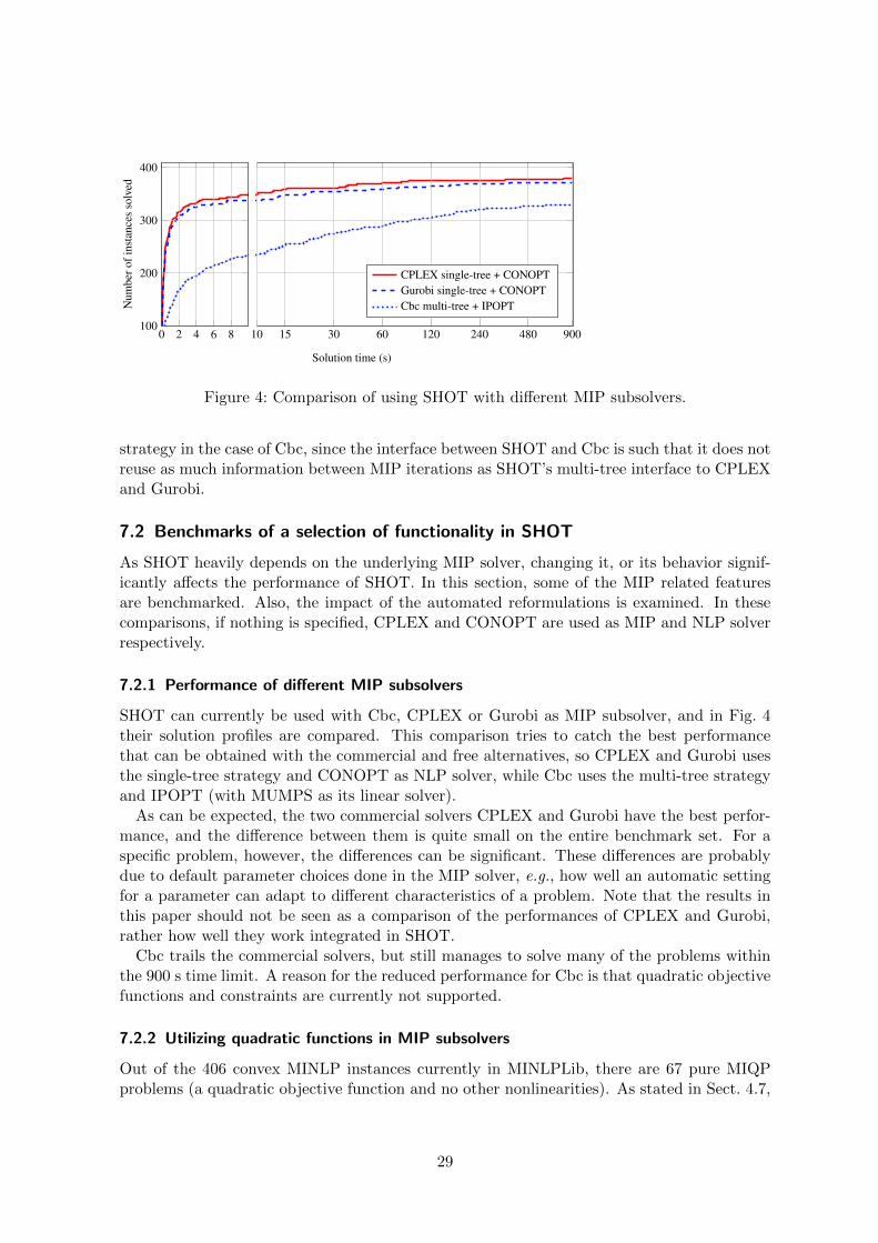
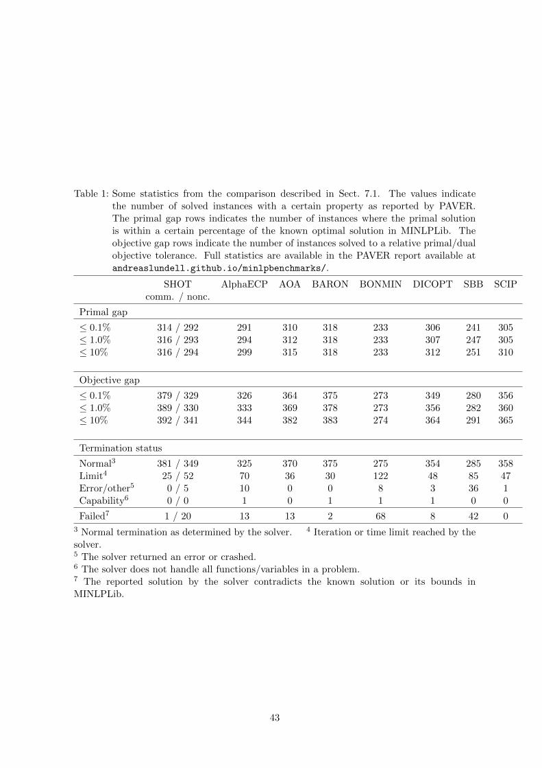
listed in App. B. The performance of the solvers was analyzed using PAVER 2.0 [11], and thegenerated PAVER reports are available at andreaslundell.github.io/minlpbenchmarks.

All comparisons were performed on a computer with an Intel Xeon 3.6 GHz processor withfour physical cores (with the possibility to process eight threads) and 32 GB memory. TheMIP solvers utilized in SHOT 1.0 was CPLEX 12.10, Gurobi 9.0 and Cbc 2.10. The NLPsubsolver selected in SHOT was CONOPT 3.17L and IPOPT 3.13.2 (with MUMPS linearsolver) for the commercial version and noncommercial version respectively. The terminationcriteria used was GAPrel = 0.1%, GAPabs = 0 and a time limit of 900 seconds.

7.1 Comparisons to other MINLP solvers

In [37], it was shown that a prerelease version of the SHOT solver (0.9.3) was very competitivewhen comparing to other convex MINLP solvers. The functionality of SHOT has been signifi-cantly extended since the publication of that paper, e.g., the entire problem handling has beenrewritten, and the automated reformulations, bound tightening and convexity identificationsteps are new. Therefore, a new comparison is conducted in this paper. The solvers includedin the comparison are the GAMS solvers AlphaECP (2.10.06), BARON (20.4.14), BONMIN(1.8), DICOPT (2), SBB (31.1.0) and SCIP (7.0). The AIMMS solver AOA (4.72.3.2) wasalso considered. For the solvers with multiple main strategies we selected one: in BONMINthe outer-approximation strategy, and for AOA the LP/NLP-based branch-and-bound strat-egy; the reason being that these strategies performed best in the benchmark provided in [37].SCIP, which is technically open-source and free for noncommercial use, does have a more re-strictive license than both BONMIN and SHOT, and cannot be used for commercial purposeswithout additional licensing. However for the sake of this comparison we classified SCIP asa noncommercial solver. Note that for academic use, SHOT can also be used freely withCPLEX and Gurobi as MIP solvers. The commercial GAMS solvers utilized CPLEX 12.10

25

and CONOPT 3.17L as subsolvers, while BONMIN used Cbc 2.10 and IPOPT 3.13.2 (withthe MUMPS linear solver). The AOA solver is implemented in AIMMS 4.72.3 and utilizedCPLEX 12.10 and CONOPT 3.14V. If the solvers had a convex strategy, or recommendedparameters for convex problems, these were used; in addition, some parameters were modi-fied to prevent the solvers to terminate prematurely. The modified parameters are listed inApp. C.

The comparisons are shown as a solution profile in Fig. 2 when considering the number ofinstances solved to a relative objective gap of 0.1%, and Fig. 3 when considering the numberof instances where he found primal solution is less than 0.1% from the solution classifiedas optimal in MINLPLib; note that the solution to only 318 of the 406 problems in thisbenchmark set are flagged as optimal in MINLPLib. Additionally, some statistics are providedin Table 1. Two versions of SHOT is included, one with commercial subsolvers (CPLEX andCONOPT) and one with open-source subsolvers (Cbc and IPOPT). This provides not onlya comparison of how the choice of subsolvers affect SHOT’s performance, but also whatperformance can be expected of a state-of-the-art open-source solver today.

7.1.1 Commercial solvers

Of the commercial solvers, It is clear that SHOT (with CPLEX and CONOPT) is verycompetitive on the whole test set, as is AOA and BARON. AOA is an implementation inAIMMS of an LP/NLP based branch-and-bound strategy. Both SHOT and AOA thus utilizea single-tree strategy with tight MIP solver integration through lazy constraint callbacks, andthis clearly illustrates the benefits of such an implementation.

BARON is a global solver, and can therefore solve problems of the more general nonconvexMINLP class. However, as the results show, it is also a very good convex MINLP solver.The convex setting for AlphaECP is used here but although the basic methods are similar(dual bounds by ECP and ESH, respectively, together with primal heuristics based on solvinginteger-fixed NLP problems), the performance of AlphaECP is not on par with SHOT in thiscomparison. Some of the reasons include that AlphaECP does not currently support solvingMIQP subproblems, nor does it have automated reformulations, bound tightening, etc.

7.1.2 Noncommercial solvers

Of the open-source solvers SHOT and BONMIN, both with Cbc and IPOPT as subsolvers,it can clearly be seen that SHOT is more efficient. In fact, the noncommercial version ofSHOT is overall more efficient than some commercial alternatives. This clearly shows thatit is possible to implement an efficient, completely free solver for convex MINLP. SCIP isa global solver, but in this comparison its convex strategy has been used since we know allproblems are convex. It is obvious that SCIP is much faster than both BONMIN and thenoncommercial version of SHOT. Also, note that the performance profile is for the entire testset, so with parameter tuning, it is possible to reduce the solution times for specific problems.Recently, there has been significant development on Cbc as well, and it can be expected thatthe performance and stability of SHOT with Cbc will increase in future versions. Anotheroption, not yet investigated, is how a single-tree version implementation of SHOT with Cbcwould work. While the choice between single- or multi-tree strategies does not seem toimpact the overall performance of SHOT as much when using CPLEX, cf., Sect. 7.2.4, it canbe assumed that the single-tree strategy will be relatively more efficient than the multi-tree

26

Commercial solvers or solvers with commercial subsolvers

0 2 4 6 8 10100

200

300

400

Solution time (s)

Num

bero

fins

tanc

esso

lved

Solution time (s)

15 30 60 120 240 480 900

AlphaECP AOA BARON DICOPT SBB SHOT comm.

Noncommercial solvers

0 2 4 6 8 10100

200

300

400

Solution time (s)

Num

bero

fins

tanc

esso

lved

Solution time (s)

15 30 60 120 240 480 900

SCIP BONMIN SHOT noncomm.

Figure 2: Solution profiles indicating the number of solved problem instances in the solverbenchmark in Section 7.1 with a relative objective gap ≤ 0.1%. In the plots, thearea between the virtual worst and virtual best solvers in each group is shaded.Also, to make it easier to compare the two plots, thin gray lines representing theperformance of the solver in the other category (noncommercial/commercial) areshown.

27

Commercial solvers or solvers with commercial subsolvers

0 2 4 6 8 10100

200

300

400

Solution time (s)

Num

bero

fins

tanc

esso

lved

Solution time (s)

15 30 60 120 240 480 900

AlphaECP AOA BARON DICOPT SBB SHOT comm.

Noncommercial solvers

0 2 4 6 8 10100

200

300

400

Solution time (s)

Num

bero

fins

tanc

esso

lved

Solution time (s)

15 30 60 120 240 480 900

SCIP BONMIN SHOT noncomm.

Figure 3: Solution profiles indicating the number of solved problem instances in the solverbenchmark in Section 7.1 with a primal gap, i.e., the relative difference to theoptimal solution in MINLPLib, ≤ 0.1%. The dashed line indicates the number ofproblems with a solution classified as optimal (318). In the plots, the area betweenthe virtual worst and virtual best solvers in each group is shaded. Also, to make iteasier to compare the two plots, thin gray lines representing the performance of thesolver in the other category (noncommercial/commercial) are shown.

28

0 2 4 6 8100

200

300

400

Solution time (s)

Num

bero

fins

tanc

esso

lved

Solution time (s)

10 15 30 60 120 240 480 900

CPLEX single-tree + CONOPTGurobi single-tree + CONOPTCbc multi-tree + IPOPT

Figure 4: Comparison of using SHOT with different MIP subsolvers.

strategy in the case of Cbc, since the interface between SHOT and Cbc is such that it does notreuse as much information between MIP iterations as SHOT’s multi-tree interface to CPLEXand Gurobi.

7.2 Benchmarks of a selection of functionality in SHOT

As SHOT heavily depends on the underlying MIP solver, changing it, or its behavior signif-icantly affects the performance of SHOT. In this section, some of the MIP related featuresare benchmarked. Also, the impact of the automated reformulations is examined. In thesecomparisons, if nothing is specified, CPLEX and CONOPT are used as MIP and NLP solverrespectively.

7.2.1 Performance of different MIP subsolvers

SHOT can currently be used with Cbc, CPLEX or Gurobi as MIP subsolver, and in Fig. 4their solution profiles are compared. This comparison tries to catch the best performancethat can be obtained with the commercial and free alternatives, so CPLEX and Gurobi usesthe single-tree strategy and CONOPT as NLP solver, while Cbc uses the multi-tree strategyand IPOPT (with MUMPS as its linear solver).

As can be expected, the two commercial solvers CPLEX and Gurobi have the best perfor-mance, and the difference between them is quite small on the entire benchmark set. For aspecific problem, however, the differences can be significant. These differences are probablydue to default parameter choices done in the MIP solver, e.g., how well an automatic settingfor a parameter can adapt to different characteristics of a problem. Note that the results inthis paper should not be seen as a comparison of the performances of CPLEX and Gurobi,rather how well they work integrated in SHOT.

Cbc trails the commercial solvers, but still manages to solve many of the problems withinthe 900 s time limit. A reason for the reduced performance for Cbc is that quadratic objectivefunctions and constraints are currently not supported.

7.2.2 Utilizing quadratic functions in MIP subsolvers

Out of the 406 convex MINLP instances currently in MINLPLib, there are 67 pure MIQPproblems (a quadratic objective function and no other nonlinearities). As stated in Sect. 4.7,

29

0 2 4 6 8200

250

300

350

400

Solution time (s)

Num

bero

fins

tanc

esso

lved

Solution time (s)

10 15 30 60 120 240 480 900

SHOT with MI(QC)QP subproblemsSHOT with MILP subproblems

Figure 5: The impact of solving MIQP or MIQCQP subproblems instead of MILP subprob-lems in SHOT as described in Section 4.7. CPLEX was used as MIP solver.

0 2 4 6 8200

250

300

350

400

Solution time (s)

Num

bero

fins

tanc

esso

lved

Solution time (s)

10 15 30 60 120 240 480 900

Seven threadsFour threadsOne thread

Figure 6: The impact of multi-threading on CPLEX with the single-tree strategy. It is clearthat utilizing more than one thread is beneficial for more difficult problems.

such problems can be directly solved by CPLEX and Gurobi. This is normally much moreefficient than utilizing iterative linearizations of the objective function to approximate itsnonlinearity since a quadratic objective can now be expressed exactly. There are also instanceswith a quadratic objective function and quadratic constraints in addition to general nonlinearconstraints. In this case, it is possible to handle the nonlinear constraints with the ESH orECP methods, while passing the quadratic objective function and/or constraints on to theMIP solver. Thus, MIQP or MIQCQP subproblems are solved instead of MILP subproblems.In Fig. 5, the impact of utilizing a MIQCQP subsolver with the multi-tree strategy has beenillustrated. CPLEX was used in this comparison, but the results are similar with Gurobi aswell. Also, using the single-tree strategy does not normally affect the performance significantlywhen considering all the 67 problems, but for individual problems the solution times may ofcourse vary. As can be seen from the figure, the impact of utilizing a MIQCQP subsolver isquite significant, and it is clear that a dedicated MI(QC)QP solver performs better for thesekind of problems than SHOT with its POA strategy.

30

0 2 4 6 8200

250

300

350

400

Solution time (s)

Num

bero

fins

tanc

esso

lved

Solution time (s)

10 15 30 60 120 240 480 900

Single-tree strategyMulti-tree strategy

Figure 7: A comparison of the performance of the single and multi-tree strategies in SHOTwhen using CPLEX as MIP solver.

7.2.3 Impact of multi-threading in the MIP solver

In Fig. 6, the impact of utilizing several threads in CPLEX is shown. The number of threadsare set at one, four and seven (the maximum number supported simultaneously by the CPUminus one). As can be expected, using more than one thread has a significant influence onthe solution time required to solve certain problem instances. For example, it takes about 74seconds to solve 350 problems with only one thread, while it takes only about 14 s and 10 sof that time to solve the same number with four and seven threads respectively. It is howeverwell-known that the performance does not normally grow linearly with the number of usedMIP solver threads and the difference between the overall performance when using four andseven threads is with regards to this benchmark negligible. However, for a newer CPU withmore cores than the one used in this comparison, the differences may be more significant.

7.2.4 Impact of MIP solution strategies on SHOT

In Fig. 7, the multi-tree and single-tree strategies in SHOT are compared using CPLEX asthe MIP solver. The multi-tree strategy performs somewhat better when considering howmany instances were solved to an objective gap below 0.1%. For simpler problems however,the single-tree strategy is significantly more efficient. A reason that the single-tree strategy isless efficient for more difficult problems is because utilizing MIP solver callbacks in CPLEXdisables functionality such as dynamic search, which might have more effect on solving moredifficult problems. Therefore, if the problem is expected to be difficult, the multi-tree strategymight be the best choice.

The results support the assumption that a multi-tree strategy can also be very competitiveif implemented efficiently. A multi-tree implementation like the one in SHOT communicatesinformation to the MIP solver, including the current primal solution point, as well as a cut-offvalue from this solution point’s objective value for pruning the branching tree. The cut-offvalue is also provided as a cut-off constraint if the objective function is linear, but this is mostlyused in SHOT’s nonconvex strategy. Also the technique to only solve some subproblems tofeasibility (cf., Sect. 4.6) and utilizing the solution pool to add multiple linearizations periteration (cf., Sect. 4.5) impact the performance of the multi-tree implementation. Anotherimportant aspect why the multi-tree strategy is so efficient is the usage of the MIP presolverin each iteration in the subsolver: Due to the fact that many of the MIP subproblems are

31

0 2 4 6 8200

250

300

350

400

Solution time (s)

Num

bero

fins

tanc

esso

lved

Solution time (s)

10 15 30 60 120 240 480 900

Subproblems solved to feasibility with solution poolSubproblems solved to optimality with solution poolSubproblems solved to optimality without solution pool

Figure 8: The impact of not utilizing the solution limit strategy described in Section 4.6 andthe MIP solution pool described in Section 4.5.

0 2 4 6 8200

250

300

350

400

Solution time (s)

Num

bero

fins

tanc

esso

lved

Solution time (s)

10 15 30 60 120 240 480 900

With reformulationsWithout reformulations

Figure 9: The impact of disabling the automatic reformulations in SHOT. Note that solvingquadratic subproblems in SHOT has been disabled.

not solved to optimality when utilizing the MIP solution limit strategy, often no branching isneeded, and the subproblems are solved during the presolving phase.

In Fig. 8, the impact of disabling these strategies are illustrated. To make the differencesclearer, the functionality to solve quadratic subproblems (MIQP or MIQCQP) were disabled,i.e., all subproblems are now linear. Differences are noticeable, e.g., disabling both the solutionpool functionality and solving the problems to optimality changes the time for solving 350instances from about 43 s to 253 s. However for simple problems, the results indicate thatit is beneficial to solve the subproblems to optimality, which can be expected as fewer butbetter linearizations are created.

7.2.5 Impact of automated reformulations

To test the impact of the automated convexity-preserving reformulations described in Sect. 4.3,these are now disabled. Also here the quadratic functionality of the MIP subsolver is disabled,i.e., only LP and MILP subproblems are solved. The solution profile compared to standardstrategy is shown in Fig. 9, and the difference is significant. This can clearly be seen as anindication that the reformulations are beneficial for a POA-based MINLP solver.

32

8 Conclusions and future work

In this paper, the SHOT solver was described in detail and its performance was thoroughlybenchmarked. The internal numerical benchmarks of the solver-specific functionality indicatethat the performance of SHOT is not due to a single feature, but a combination of many dif-ferent strategies that together result in a well-performing solver. Thus, it can be summarizedthat SHOT builds on and extends 30 years worth of research on POA methods for MINLP.One of the main features of POA-based solvers is that they rely heavily on the subsolvers uti-lized, and this is especially true for the single-tree strategy in SHOT. Although the numericalcomparison between the single- and multi-tree strategies did not result in a clear winner, itshould be mentioned, that a large part of the convex problems in MINLPLib are very easyto solve with both strategies as long as an efficient MIP solver is utilized. For the multi-treeimplementation, there is not much more possibilities for further enhancing the performanceby tighter integration with the MIP solver. However, for the single-tree implementation,there are still many aspects to consider including generating hyperplane cuts also in relaxedsolution points, and to only add cuts locally in the search tree.

For SHOT, the next major development steps are to implement more primal heuristicsand to include more automated convexity preserving reformulations. These improvementsare meant to enhance the performance especially for more demanding problems. AlthoughSHOT 1.0 has some basic, mainly heuristic, nonconvex capabilities, we plan to add morefunctionality, based on lifting reformulations, for nonconvex MINLP in the feature. In additionto being important in itself, convex MINLP can also then be used as a tool for solvingnonconvex problems by reformulating such problems into convex MINLP problems [50, 51,59, 60]. In certain aspects, this mimics how MIP problems can be used in POA to solveconvex MINLP problems. Of course, this is much more difficult in practice due to the factthat several convex MINLP problems are solved in sequence to find the optimal solution to anonconvex MINLP problems. Also, the reformulated problems grow not only in the number ofadditional linear constraints as in POA, but also in the number of auxiliary variables neededfor the reformulations. However, since a tight integration of these reformulations with SHOTis possible, we assume this will be an efficient way to solve certain classes of nonconvex MINLPproblems.

Acknowledgements

The authors want to thank both GAMS (especially S. Vigerske and M. Bussieck) and AIMMS(especially M. Hunting) for their support. A. Lundell also wants to express his gratitude forthe financial support from the Magnus Ehrnrooth Foundation, as well as the Ruth and Nils-Erik Stenback Foundation. Similarly, J. Kronqvist also wants to express his gratitude for thefinancial support fron the Newton International Fellowship by the Royal Society(NIF\R1\82194)and the Swedish Cultural Foundation in Finland.

References

[1] Abhishek, K., Leyffer, S., Linderoth, J., 2010. FilMINT: An outer approximation-basedsolver for convex mixed-integer nonlinear programs. INFORMS Journal on Computing22, 555–567.

33

[2] Alefeld, G., Potra, F.A., Shi, Y., 1995. Algorithm 748: Enclosing zeros of continuousfunctions. ACM Transactions on Mathematical Software 21, 327–344.

[3] Bell, B.M., 2012. Cppad: a package for C++ algorithmic differentiation. ComputationalInfrastructure for Operations Research 57.

[4] Belotti, P., 2009. Couenne: A user’s manual. Technical Report. Lehigh University.

[5] Bernal, D.E., Vigerske, S., Trespalacios, F., Grossmann, I.E., 2020. Improving the per-formance of DICOPT in convex MINLP problems using a feasibility pump. OptimizationMethods and Software 35, 171–190.

[6] Berthold, T., Lodi, A., Salvagnin, D., 2017. Ten years of feasibility pump and count-ing. Technical Report. Polytechnique Montreal, Departement de Mathematiques e GenieIndustriel.

[7] Bisschop, J., 2006. AIMMS optimization modeling. Lulu.com.

[8] Bonami, P., Biegler, L.T., Conn, A.R., Cornuejols, G., Grossmann, I.E., Laird, C.D.,Lee, J., Lodi, A., Margot, F., Sawaya, N., Wachter, A., 2008. An algorithmic frameworkfor convex mixed integer nonlinear programs. Discrete Optimization 5, 186–204.

[9] Bonami, P., Cornuejols, G., Lodi, A., Margot, F., 2009. A feasibility pump for mixedinteger nonlinear programs. Mathematical Programming 119, 331–352.

[10] Brook, A., Kendrick, D., Meeraus, A., 1988. GAMS, a user’s guide. ACM SignumNewsletter 23, 10–11.

[11] Bussieck, M., Dirkse, S., Vigerske, S., 2014. PAVER 2.0: An open source environment forautomated performance analysis of benchmarking data. Journal of Global Optimization59, 259–275.

[12] Bussieck, M.R., Meeraus, A., 2004. General Algebraic Modeling System (GAMS), in:Kallrath, J. (Ed.), Modeling Languages in Mathematical Optimization. Springer US,Boston, MA, pp. 137–157.

[13] Bussieck, M.R., Vigerske, S., 2010. MINLP solver software, in: Wiley Encyclopedia ofOperations Research and Management Science. Wiley Online Library, pp. 1–12.

[14] Ceccon, F., Siirola, J.D., Misener, R., 2019. SUSPECT: MINLP special structure detec-tor for pyomo. Optimization Letters 14, 801–814.

[15] Dakin, R.J., 1965. A tree-search algorithm for mixed integer programming problems.The Computer Journal 8, 250–255.

[16] Drud, A.S., 1994. CONOPT — a large-scale GRG code. ORSA Journal on computing6, 207–216.

[17] Dunning, I., Huchette, J., Lubin, M., 2017. JuMP: A modeling language for mathematicaloptimization. SIAM Review 59, 295–320.

[18] Duran, M.A., Grossmann, I.E., 1986. An outer-approximation algorithm for a class ofmixed-integer nonlinear programs. Mathematical Programming 36, 307–339.

34

[19] Fletcher, R., Leyffer, S., 1994. Solving mixed integer nonlinear programs by outer ap-proximation. Mathematical programming 66, 327–349.

[20] Forrest, J., Lougee-Heimer, R., 2005. CBC User Guide. URL: http://www.coin-or.org/Cbc.

[21] Fourer, R., Gay, D., Kernighan, B., 1993. AMPL. Boyd & Fraser Danvers.

[22] Fourer, R., Gay, D.M., Kernighan, B.W., 1990. A modeling language for mathematicalprogramming. Management Science 36, 519–554.

[23] Fourer, R., Ma, J., Martin, K., 2010. OSiL: An instance language for optimization.Computational Optimization and Applications 45, 181–203.

[24] GAMS Development Corp., 2018. SBB user’s manual. URL: https://www.gams.com/latest/docs/S_SBB.html.

[25] Gassmann, H., Ma, J., Martin, K., Sheng, W., 2015. Optimization Services2.10 User’s Manual. URL: http://projects.coin-or.org/svn/OS/trunk/OS/doc/

osUsersManual.pdf.

[26] Geoffrion, A.M., 1972. Generalized Benders decomposition. Journal of OptimizationTheory and Applications 10, 237–260.

[27] Grossmann, I.E., 2002. Review of nonlinear mixed-integer and disjunctive programmingtechniques. Optimization and Engineering 3, 227–252.

[28] Grossmann, I.E., Viswanathan, J., Vecchietti, A., Raman, R., Kalvelagen, E., et al., 2002.GAMS/DICOPT: A discrete continuous optimization package. GAMS Corporation Inc.

[29] Guennebaud, G., Jacob, B., et al., 2010. Eigen v3. URL: http://eigen.tuxfamily.org.

[30] Gupta, O.K., Ravindran, A., 1985. Branch and bound experiments in convex nonlinearinteger programming. Management Science 31, 1533–1546.

[31] Hart, W.E., Laird, C., Watson, J.P., Woodruff, D.L., 2012. Pyomo - OptimizationModeling in Python. 1st ed., Springer.

[32] Hijazi, H., Bonami, P., Ouorou, A., 2014. An outer-inner approximation for separablemixed-integer nonlinear programs. INFORMS Journal on Computing 26, 31–44.

[33] HSL, 2018. A collection of Fortran codes for large-scale scientific computation. URL:http://www.hsl.rl.ac.uk.

[34] Hunting, M., 2011. The AIMMS outer approximation algorithm for MINLP. TechnicalReport. AIMMS B.V.

[35] Kroger, O., Coffrin, C., Hijazi, H., Nagarajan, H., 2018. Juniper: An Open-SourceNonlinear Branch-and-Bound Solver in Julia. arXiv preprint: 1804.07332.

[36] Kronqvist, J., Bernal, D.E., Grossmann, I.E., 2020. Using regularization and second orderinformation in outer approximation for convex MINLP. Mathematical Programming 180,285––310.

35

[37] Kronqvist, J., Bernal, D.E., Lundell, A., Grossmann, I.E., 2019. A review and comparisonof solvers for convex MINLP. Optimization and Engineering 20, 397––455.

[38] Kronqvist, J., Lundell, A., Westerlund, T., 2015. The extended supporting hyperplanealgorithm for convex mixed-integer nonlinear programming. Journal of Global Optimiza-tion 64, 249–272.

[39] Kronqvist, J., Lundell, A., Westerlund, T., 2017. A center-cut algorithm for solvingconvex mixed-integer nonlinear programming problems, in: Computer Aided ChemicalEngineering. Elsevier. volume 40, pp. 2131–2136.

[40] Kronqvist, J., Lundell, A., Westerlund, T., 2018. Reformulations for utilizing separabilitywhen solving convex MINLP problems. Journal of Global Optimization 71, 571––592.

[41] Lastusilta, T., Bussieck, M.R., Westerlund, T., 2009. An experimental study of theGAMS/AlphaECP MINLP solver. Industrial & Engineering Chemistry Research 48,7337–7345.

[42] Leyffer, S., 1993. Deterministic methods for mixed integer nonlinear programming. Ph.D.thesis. University of Dundee.

[43] Liberti, L., 2009. Reformulation techniques in mathematical programming. HDR thesis.

[44] Lin, Y., Schrage, L., 2009. The global solver in the LINDO API. Optimization Methods& Software 24, 657–668.

[45] Lubin, M., Yamangil, E., Bent, R., Vielma, J.P., 2016. Extended formulations inmixed-integer convex programming, in: Louveaux, Q., Skutella, M. (Eds.), Integer Pro-gramming and Combinatorial Optimization: 18th International Conference, IPCO 2016,Springer International Publishing. pp. 102–113.

[46] Lundell, A., 2009. Transformation Techniques for Signomial Functions in Global Opti-mization. Ph.D. thesis. Abo Akademi University.

[47] Lundell, A., Kronqvist, J., Westerlund, T., 2016. Improvements to the supporting hy-perplane optimization toolkit solver for convex MINLP, in: XIII Global OptimizationWorkshop GOW’16, pp. 101–104.

[48] Lundell, A., Kronqvist, J., Westerlund, T., 2017. SHOT – a global solver for convexMINLP in Wolfram Mathematica, in: Computer Aided Chemical Engineering. Elsevier.volume 40, pp. 2137–2142.

[49] Lundell, A., Kronqvist, J., Westerlund, T., 2018. The Supporting Hyperplane Optimiza-tion Toolkit. URL: http://www.github.com/coin-or/shot.

[50] Lundell, A., Westerlund, J., Westerlund, T., 2009. Some transformation techniques withapplications in global optimization. Journal of Global Optimization 43, 391–405.

[51] Lundell, A., Westerlund, T., 2018. Solving global optimization problems using reformula-tions and signomial transformations. Computers & Chemical Engineering 116, 122–134.

36

[52] Mahajan, A., Leyffer, S., Linderoth, J., Luedtke, J., Munson, T., 2017. Minotaur: AMixed-Integer Nonlinear Optimization Toolkit. Preprint, Optimization Online URL:http://www.optimization-online.org/DB_FILE/2017/10/6275.pdf.

[53] Melo, W., Fampa, M., Raupp, F., 2020. An overview of MINLP algorithms and theirimplementation in Muriqui Optimizer. Annals of Operations Research , 217–241.

[54] Messine, F., 2004. Deterministic global optimization using interval constraint propaga-tion techniques. RAIRO-Operations Research 38, 277–293.

[55] MINLPLib, 2020. Mixed-integer nonlinear programming library. URL: http://www.minlplib.org/. Accessed January 6 2020.

[56] Misener, R., Floudas, C.A., 2014. ANTIGONE: Algorithms for continuous/integer globaloptimization of nonlinear equations. Journal of Global Optimization 59, 503–526.

[57] Muts, P., Nowak, I., Hendrix, E.M., 2020. The decomposition-based outer approxi-mation algorithm for convex mixed-integer nonlinear programming. Journal of GlobalOptimization , 1–22.

[58] Nagarajan, H., Lu, M., Wang, S., Bent, R., Sundar, K., 2019. An adaptive, multivariatepartitioning algorithm for global optimization of nonconvex programs. Journal of GlobalOptimization doi:10.1007/s10898-018-00734-1.

[59] Nowak, I., Breitfeld, N., Hendrix, E.M., Njacheun-Njanzoua, G., 2018. Decomposition-based inner-and outer-refinement algorithms for global optimization. Journal of GlobalOptimization , 305–321.

[60] Porn, R., Harjunkoski, I., Westerlund, T., 1999. Convexification of different classes ofnon-convex MINLP problems. Computers and Chemical Engineering 23, 439–448.

[61] Quesada, I., Grossmann, I.E., 1992. An LP/NLP based branch and bound algorithm forconvex MINLP optimization problems. Computers & Chemical Engineering 16, 937–947.

[62] Sahinidis, N.V., 1996. BARON: A general purpose global optimization software package.Journal of Global Optimization 8, 201–205.

[63] Schaling, B., 2014. The Boost C++ Libraries (2nd edition). XML Press.

[64] Schichl, H., Neumaier, A., 2005. Interval analysis on directed acyclic graphs for globaloptimization. Journal of Global Optimization 33, 541–562.

[65] Slater, M., 1950. Lagrange multipliers revisited. Technical Report. Cowles Foundationfor Research in Economics, Yale University.

[66] Su, L., Tang, L., Bernal, D.E., Grossmann, I.E., 2018. Improved quadratic cuts for convexmixed-integer nonlinear programs. Computers & Chemical Engineering 109, 77–95.

[67] Su, L., Tang, L., Grossmann, I.E., 2015. Computational strategies for improved minlpalgorithms. Computers & Chemical Engineering 75, 40–48.

[68] Tasseff, B., Coffrin, C., Wachter, A., Laird, C., 2019. Exploring benefits of linear solverparallelism on modern nonlinear optimization applications. arXiv:1909.08104.

37

[69] Tawarmalani, M., Sahinidis, N.V., 2005. A polyhedral branch-and-cut approach to globaloptimization. Mathematical programming 103, 225–249.

[70] Trespalacios, F., Grossmann, I.E., 2014. Review of mixed-integer nonlinear and general-ized disjunctive programming methods. Chemie Ingenieur Technik 86, 991–1012.

[71] Vigerske, S., Gleixner, A., 2018. SCIP: Global optimization of mixed-integer nonlinearprograms in a branch-and-cut framework. Optimization Methods and Software 33, 563–593.

[72] Wachter, A., Biegler, L.T., 2006a. On the implementation of an interior-point filter line-search algorithm for large-scale nonlinear programming. Mathematical Programming106, 25–57.

[73] Wachter, A., Biegler, L.T., 2006b. On the implementation of an interior-point filter line-search algorithm for large-scale nonlinear programming. Mathematical programming106, 25–57.

[74] Westerlund, T., Eronen, V.P., Makela, M.M., 2018. On solving generalized convexMINLP problems using supporting hyperplane techniques. Journal of Global Optimiza-tion 71, 981–1011.

[75] Westerlund, T., Lastusilta, T., 2008. AlphaECP GAMS user’s manual. URL: http://www.gams.com/latest/docs/S_ALPHAECP.html.

[76] Westerlund, T., Lundqvist, K., 2005. Alpha-ECP, An Interactive MINLP-Solver Basedon the Extended Cutting Plane Method. Technical Report. Abo Akademi University.

[77] Westerlund, T., Pettersson, F., 1995. An extended cutting plane method for solvingconvex MINLP problems. Computers & Chemical Engineering 19, 131–136.

[78] Westerlund, T., Porn, R., 2002. Solving pseudo-convex mixed-integer problems by cut-ting plane techniques. Optimization and Engineering 3, 253–280.

Appendix A: A cutting plane-based algorithm for locating aninterior point

To find the interior point to use as end point in the root searches in the ESH algorithm imple-mented in SHOT, cf., Sect. 4.4, the minimax problem Prob. (MM) is considered. An optimalor feasible interior point can be obtained with the tailor-made minimax solver described below:

Specify a maximum number of iterations and a relative (εMMrel ) and absolute (εMM

abs ) ter-mination tolerance for the objective function. Set GAPMM

rel := ∞ and GAPMMabs := ∞, and

determine a maximal number of iterations KMMmax ≥ 2. Set the iteration index k := 1.

1. Reformulate the original MINLP problem, Prob. (P), into a minimax problem of thetype in Prob. (MM). Denote the function G(x) = maxj gj(x), i.e., the maximum errorof all nonlinear constraints functions in the original problem.

2. Create a copy of the minimax problem without the nonlinear constraints, i.e., an LPproblem.

38

3. Solve the LP problem. If the subproblem can not be solved to optimality, set the flagMinimaxStatus to failure and go to Step 5; otherwise obtain the solution (x1, ν1),and denote OBJLP = ν1.

4. Repeat while k < KMMmax .

a) Increase the iteration counter, i.e., set k := k + 1.

b) Solve the LP problem. If the subproblem could not be solved to optimality, setMinimaxStatus to failure and go to Step 5; otherwise, obtain the solution (xk, νk)and set OBJLP = νk.

c) Solve the following one-dimensional minimization problem:

λk = argminλ∈[0,1]G (λxk + (1− λ)xk−1)

and calculate the solution point as xLS = λkxk+(1−λk)xk−1. Calculate OBJLS =G(xLS).

d) Calculate the absolute and relative difference in objective values between the LPand line search:

GAPMMabs = |OBJLP −OBJLS|, and GAPMM

rel =|OBJLP −OBJLS||OBJLP|+ 10−10

.

If OBJLP < 0, and GAPMMrel < εMM

rel or GAPMMabs < εMM

abs , set MinimaxStatus tosuccess and go to Step 5.

e) Select the constraint function with the largest error in the point xLS, i.e., find

j′ = argmaxj gj(xLS)

and add the following cutting plane to the LP problem

gj′(xLS) +∇gj′ (xLS))T (x− xLS) ≤ 0.

Note that it is also possible to generate cutting planes for more than one of theviolated constraints.

5. Termination: If MinimaxStatus is success, return with the status success and theinterior point xLS, otherwise with status failure.

Appendix B: Included problems in the benchmark

The following 406 problems were used in the benchmark in Sect. 7. They are the instancesthat are identified as convex in MINLPLib, with at least one nonlinearity (in the objectivefunction or constraints), and at least one discrete (binary or integer) variable. Of these,the 67 problems marked with an ∗ have only a quadratic objective function and no furthernonlinearities in the constraints, i.e., they are MIQP problems.

alan∗, ball mk2 10, ball mk2 30, ball mk3 10, ball mk3 20, ball mk3 30, ball mk4 05,ball mk4 10, ball mk4 15, batch, batch0812, batchdes, batchs101006m, batchs121208m,batchs151208m, batchs201210m, clay0203h, clay0203hfsg, clay0203m, clay0204h,

39

clay0204hfsg, clay0204m, clay0205h, clay0205hfsg, clay0205m, clay0303h,clay0303hfsg, clay0303m, clay0304h, clay0304hfsg, clay0304m, clay0305h,clay0305hfsg, clay0305m, color lab2 4x0∗, color lab6b 4x20∗, cvxnonsep normcon20,cvxnonsep normcon20r, cvxnonsep normcon30, cvxnonsep normcon30r,cvxnonsep normcon40, cvxnonsep normcon40r, cvxnonsep nsig20, cvxnonsep nsig20r,cvxnonsep nsig30, cvxnonsep nsig30r, cvxnonsep nsig40, cvxnonsep nsig40r,cvxnonsep pcon20, cvxnonsep pcon20r, cvxnonsep pcon30, cvxnonsep pcon30r,cvxnonsep pcon40, cvxnonsep pcon40r, cvxnonsep psig20, cvxnonsep psig20r,cvxnonsep psig30, cvxnonsep psig30r, cvxnonsep psig40, cvxnonsep psig40r, du-opt∗,du-opt5∗, enpro48pb, enpro56pb, ex1223, ex1223a∗, ex1223b, ex4∗, fac1, fac2, fac3∗,flay02h, flay02m, flay03h, flay03m, flay04h, flay04m, flay05h, flay05m, flay06h,flay06m, fo7, fo7 2, fo7 ar25 1, fo7 ar2 1, fo7 ar3 1, fo7 ar4 1, fo7 ar5 1, fo8,fo8 ar25 1, fo8 ar2 1, fo8 ar3 1, fo8 ar4 1, fo8 ar5 1, fo9, fo9 ar25 1, fo9 ar2 1,fo9 ar3 1, fo9 ar4 1, fo9 ar5 1, gams01, gbd∗, hybriddynamic fixed∗, ibs2, jit1, m3,m6, m7, m7 ar25 1, m7 ar2 1, m7 ar3 1, m7 ar4 1, m7 ar5 1, meanvar-orl400 05 e 8∗,meanvarx∗, meanvarxsc∗, netmod dol1∗, netmod dol2∗, netmod kar1∗, netmod kar2∗,no7 ar25 1, no7 ar2 1, no7 ar3 1, no7 ar4 1, no7 ar5 1, nvs03, nvs10, nvs11, nvs12,nvs15∗, o7, o7 2, o7 ar25 1, o7 ar2 1, o7 ar3 1, o7 ar4 1, o7 ar5 1, o8 ar4 1, o9 ar4 1,pedigree ex1058, pedigree ex485, pedigree ex485 2, pedigree sim2000,pedigree sim400, pedigree sp top4 250, pedigree sp top4 300,pedigree sp top4 350tr, pedigree sp top5 200, pedigree sp top5 250, portfol buyin,portfol card, portfol classical050 1, portfol classical200 2, portfol roundlot,procurement2mot, ravempb, risk2bpb, rsyn0805h, rsyn0805hfsg, rsyn0805m,rsyn0805m02h, rsyn0805m02hfsg, rsyn0805m02m, rsyn0805m03h, rsyn0805m03hfsg,rsyn0805m03m, rsyn0805m04h, rsyn0805m04hfsg, rsyn0805m04m, rsyn0810h,rsyn0810hfsg, rsyn0810m, rsyn0810m02h, rsyn0810m02hfsg, rsyn0810m02m,rsyn0810m03h, rsyn0810m03hfsg, rsyn0810m03m, rsyn0810m04h, rsyn0810m04hfsg,rsyn0810m04m, rsyn0815h, rsyn0815hfsg, rsyn0815m, rsyn0815m02h, rsyn0815m02hfsg,rsyn0815m02m, rsyn0815m03h, rsyn0815m03hfsg, rsyn0815m03m, rsyn0815m04h,rsyn0815m04hfsg, rsyn0815m04m, rsyn0820h, rsyn0820hfsg, rsyn0820m, rsyn0820m02h,rsyn0820m02hfsg, rsyn0820m02m, rsyn0820m03h, rsyn0820m03hfsg, rsyn0820m03m,rsyn0820m04h, rsyn0820m04hfsg, rsyn0820m04m, rsyn0830h, rsyn0830hfsg, rsyn0830m,rsyn0830m02h, rsyn0830m02hfsg, rsyn0830m02m, rsyn0830m03h, rsyn0830m03hfsg,rsyn0830m03m, rsyn0830m04h, rsyn0830m04hfsg, rsyn0830m04m, rsyn0840h,rsyn0840hfsg, rsyn0840m, rsyn0840m02h, rsyn0840m02hfsg, rsyn0840m02m,rsyn0840m03h, rsyn0840m03hfsg, rsyn0840m03m, rsyn0840m04h, rsyn0840m04hfsg,rsyn0840m04m, slay04h∗, slay04m∗, slay05h∗, slay05m∗, slay06h∗, slay06m∗, slay07h∗,slay07m∗, slay08h∗, slay08m∗, slay09h∗, slay09m∗, slay10h∗, slay10m∗,smallinvDAXr1b010-011, smallinvDAXr1b020-022, smallinvDAXr1b050-055,smallinvDAXr1b100-110, smallinvDAXr1b150-165, smallinvDAXr1b200-220,smallinvDAXr2b010-011, smallinvDAXr2b020-022, smallinvDAXr2b050-055,smallinvDAXr2b100-110, smallinvDAXr2b150-165, smallinvDAXr2b200-220,smallinvDAXr3b010-011, smallinvDAXr3b020-022, smallinvDAXr3b050-055,smallinvDAXr3b100-110, smallinvDAXr3b150-165, smallinvDAXr3b200-220,smallinvDAXr4b010-011, smallinvDAXr4b020-022, smallinvDAXr4b050-055,smallinvDAXr4b100-110, smallinvDAXr4b150-165, smallinvDAXr4b200-220,smallinvDAXr5b010-011, smallinvDAXr5b020-022, smallinvDAXr5b050-055,

40

smallinvDAXr5b100-110, smallinvDAXr5b150-165, smallinvDAXr5b200-220,squfl010-025∗, squfl010-040∗, squfl010-080∗, squfl015-060∗, squfl015-080∗,squfl020-040∗, squfl020-050∗, squfl020-150∗, squfl025-025∗, squfl025-030∗,squfl025-040∗, squfl030-100∗, squfl030-150∗, squfl040-080∗, sssd08-04, sssd12-05,sssd15-04, sssd15-06, sssd15-08, sssd16-07, sssd18-06, sssd18-08, sssd20-04,sssd20-08, sssd22-08, sssd25-04, sssd25-08, st e14, st miqp1∗, st miqp2∗, st miqp3∗,st miqp4∗, st miqp5∗, st test1∗, st test2∗, st test3∗, st test4∗, st test5∗, st test6∗,st test8∗, st testgr1∗, st testgr3∗, st testph4∗, stockcycle, syn05h, syn05hfsg,syn05m, syn05m02h, syn05m02hfsg, syn05m02m, syn05m03h, syn05m03hfsg, syn05m03m,syn05m04h, syn05m04hfsg, syn05m04m, syn10h, syn10hfsg, syn10m, syn10m02h,syn10m02hfsg, syn10m02m, syn10m03h, syn10m03hfsg, syn10m03m, syn10m04h,syn10m04hfsg, syn10m04m, syn15h, syn15hfsg, syn15m, syn15m02h, syn15m02hfsg,syn15m02m, syn15m03h, syn15m03hfsg, syn15m03m, syn15m04h, syn15m04hfsg, syn15m04m,syn20h, syn20hfsg, syn20m, syn20m02h, syn20m02hfsg, syn20m02m, syn20m03h,syn20m03hfsg, syn20m03m, syn20m04h, syn20m04hfsg, syn20m04m, syn30h, syn30hfsg,syn30m, syn30m02h, syn30m02hfsg, syn30m02m, syn30m03h, syn30m03hfsg, syn30m03m,syn30m04h, syn30m04hfsg, syn30m04m, syn40h, syn40hfsg, syn40m, syn40m02h,syn40m02hfsg, syn40m02m, syn40m03h, syn40m03hfsg, syn40m03m, syn40m04h,syn40m04hfsg, syn40m04m, synthes1, synthes2, synthes3, tls12, tls2, tls4, tls5, tls6,tls7, unitcommit1∗, unitcommit 200 100 1 mod 8∗, unitcommit 200 100 2 mod 8∗,unitcommit 50 20 2 mod 8∗, watercontamination0202∗, watercontamination0202r∗,watercontamination0303∗, watercontamination0303r∗

Appendix C: Used solver options in the benchmark

In the comparison in Sect. 7.1, the goal was to use the default solver options as much aspossible. However, several of the solvers have certain default parameter values that makesthem terminate prematurely, and these were then increased to avoid this behavior. Alsoconvex strategies are activated for solvers supporting this, and if the solver has recommendedparameters for convex problems, these were used. The used parameters are more or less thesame as in [37], and are explained further there.

Name Value

General GAMS

MIP CPLEXthreads 7optcr 0.001optca 0nodlim 108

domlim 108

iterlim 108

reslim 900

AlphaECP

ECPmaster 1

AOA

41

IsConvex 1IterationMax 107

RelativeOptimalityTolerance 0.1TimeLimit 900

BONMIN

bonmin.algorithm B-OAbonmin.time limit 900

DICOPT

convex 1stop 1maxcycles 108

infeasder 1nlpoptfile 1

SBB

memnodes 5 · 107

rootsolver CONOPT.1

SCIP

constraints/nonlinear/assumeconvex true

SHOT

Dual.MIP.NumberOfThreads 7Dual.MIP.Solver 0–2 (depending on MIP solver)Termination.ObjectiveGap.Absolute 0Termination.ObjectiveGap.Relative 0.001Termination.TimeLimit 900

CONOPT (GAMS)

rtmaxv 1030

42

Table 1: Some statistics from the comparison described in Sect. 7.1. The values indicatethe number of solved instances with a certain property as reported by PAVER.The primal gap rows indicates the number of instances where the primal solutionis within a certain percentage of the known optimal solution in MINLPLib. Theobjective gap rows indicate the number of instances solved to a relative primal/dualobjective tolerance. Full statistics are available in the PAVER report available atandreaslundell.github.io/minlpbenchmarks/.

SHOT AlphaECP AOA BARON BONMIN DICOPT SBB SCIPcomm. / nonc.

Primal gap

≤ 0.1% 314 / 292 291 310 318 233 306 241 305≤ 1.0% 316 / 293 294 312 318 233 307 247 305≤ 10% 316 / 294 299 315 318 233 312 251 310

Objective gap

≤ 0.1% 379 / 329 326 364 375 273 349 280 356≤ 1.0% 389 / 330 333 369 378 273 356 282 360≤ 10% 392 / 341 344 382 383 274 364 291 365

Termination status

Normal3 381 / 349 325 370 375 275 354 285 358Limit4 25 / 52 70 36 30 122 48 85 47Error/other5 0 / 5 10 0 0 8 3 36 1Capability6 0 / 0 1 0 1 1 1 0 0

Failed7 1 / 20 13 13 2 68 8 42 03 Normal termination as determined by the solver. 4 Iteration or time limit reached by thesolver.5 The solver returned an error or crashed.6 The solver does not handle all functions/variables in a problem.7 The reported solution by the solver contradicts the known solution or its bounds inMINLPLib.

43