Applied Acoustics 73 (2012) 184–189

Contents lists available at SciVerse ScienceDirect

Applied Acoustics

journal homepage: www.elsevier .com/locate /apacoust

Technical Note

The technique of active/inactive finite elements for the analysis and optimizationof acoustical chambers

Renato Barbieri a,c, Nilson Barbieri a,b,⇑a Pontifícia Universidade Católica do Paraná – PUCPR, Rua Imaculada Conceição, CEP: 80215-901, 1155 Curitiba, Paraná, Brazilb Universidade Tecnológica Federal do Paraná – UTFPR, Rua Sete de Setembro, CEP: 80230-901, 3165 Curitiba, Paraná, Brazilc Faculdade de Engenharia de Joinville, Campus Universitário s/n, CEP: 89224-100, Joinville, SC, Brazil

a r t i c l e i n f o a b s t r a c t

Article history:Received 18 April 2011Received in revised form 27 April 2011Accepted 15 August 2011Available online 7 September 2011

Keywords:Active finite elementGenetic algorithmOptimizationAcoustical chamber

0003-682X/$ - see front matter � 2011 Elsevier Ltd.doi:10.1016/j.apacoust.2011.08.002

⇑ Corresponding author at: Pontifícia UniversidadeRua Imaculada Conceição, CEP: 80215-901, 1155 Cur41 3271 2211; fax: +55 41 3271 1349.

E-mail addresses: renato.barbieri@pucpr.br (R.pucpr.br (N. Barbieri).

In this work are investigated two topics associated with numerical calculations of the transmission loss inacoustical silencers: analysis of acoustic chambers employing active/inactive finite elements and its opti-mization using the GA (genetic algorithm) with integer variables. The technical information on the use ofactive/inactive elements and the definition of all the design variables used for the entire control of thefinite element mesh are detailed. Although simple, the numerical results for the examples analyzed showexcellent convergence achieved with the combination of these two techniques for the optimization ofsymmetrical acoustic chambers.

� 2011 Elsevier Ltd. All rights reserved.

1. Introduction

The transmission loss, TL(x), can be used to define the problemof optimization of acoustic chambers (mufflers) as [1,2]:

Maximize or Minimize ðTLðxÞÞSubject to xjL 6 xj 6 xjU j ¼ 1;2;3; . . . ;nd

ð1Þ

where f(TL(x)) is the objective function that depends of the excita-tion frequency x and nd is the number of design variables xj withlower limit xjL and upper limit xjU.

To perform the optimization of the acoustic chamber on dis-crete frequencies is defined an objective function with discrete val-ues of the transmission loss as:

f ðx1;x2; . . . ;xnÞ ¼Xn

i¼1

aiTLðxiÞ ð2Þ

where ai represents a positive penalty parameter defined with thepurpose of enhancing the value of transmission loss in a specific fre-quency xi.

For the optimization in many frequency ranges the objectivefunction can be written using the average transmission loss in

All rights reserved.

Católica do Paraná – PUCPR,itiba, Paraná, Brazil. Tel.: +55

Barbieri), nilson.barbieri@

different frequency ranges. Mathematically this function is ex-pressed in the following way [3]:

f ðDx1;Dx2; . . . ;DxnÞ ¼Xn

i¼1

aiTLðDxiÞ ð3Þ

where

TLðDxiÞ ¼1

Dxi

Z xiU

xiL

TLðxÞdx ð4Þ

and ai represents a positive penalty parameter defined with thepurpose of enhancing the value of transmission loss in a specific fre-quency range, Dxi = xiU �xiL and the pair (xiU, xiL) represents theupper and lower frequencies of the range Dxi.

After selecting an appropriate objective function and the defini-tion of design variables with their limits, the mathematicalproblem defined in Eq. (1) can be solved using traditional optimi-zation methods described in literature.

In this work was used the finite element method to evaluate theobjective function together with the concept of active/inactivefinite elements to make the control of the mesh. The method ofGA with integer variables was used to perform the optimizationcalculations and the great advantage of this approach is thereduced processing time. All methodology applied in the optimiza-tion process with use of active/inactive elements and the definitionof design integer variables used in the GA are detailed later in thispaper. Although simple, the numerical examples shown in this

x1,x2,x3,...,xnd

Fig. 1. Mesh of finite elements and the design domain.

(a)

(b)

R. Barbieri, N. Barbieri / Applied Acoustics 73 (2012) 184–189 185

paper are to point out the quality of the results obtained with thisapproach.

Fig. 3. Uncoupled nodes during the optimization process. (a) Mesh with linearfinite elements and (b) mesh with quadratic finite elements.

2. The control of the mesh and the definition of design variables

After the construction of a homogeneous mesh of finite ele-ments is defined a region where it want to control the geometryin order to optimize the muffler design. Fig. 1 shows a shaded do-main (composed to nd columns with 10 finite elements percolumn. This is the design domain.

Analogous to the process of topology optimization widely usedin structural optimization, recently used by [4] for mufflers, thefinite element within the design domain are called to active orinactive elements. The active elements are those where the Helm-holtz equation is usually modeled with FEM and inactive elementsare those where the characteristic matrices of finite element arenull.

Each column in the design domain has Nj elements that corre-sponds to the upper limit of the design variable xj, j = 1, 2, . . ., nd.In Fig. 1, Nj = 10 for any column.

The design variables are used to define the number of inactiveelements in each column of the design domain. Thus each xj is aninteger variable and 0 6 xj 6 Nj. Fig. 2 shows that xm = 8 indicatingthat there are only 8 inactive elements (filled with black color) inthe column m = 5 of the design domain.

After assembling all the elements, some rows and columns ofthe finite element matrix (after assembly) can have all its elementsnull. These rows and columns are associated to the nodes insidethe design domain that belong only to inactive elements. There-fore, to avoid the singularity of the final system of equations is suf-ficient to specify to these diagonals any nonzero value. Thisprocedure does not change the result of the analysis, because thesenodes are completely uncoupled (inactive node) of the other nodesof the mesh and pertain to inactive elements that are not post-processed. In Fig. 3a and b are illustrated examples of this situationto meshes build with linear and quadratic elements, respectively.These figures show the shaded inactive elements and inactive

x5=8

Fig. 2. Inactive elements in the column m (filled with black color).

nodes filled with black color. However, the approach describedabove can be applied to any other type of element.

During all the optimization process the finite element meshremains unchanged, but for each evaluation of the objective func-tion some active elements may become inactive and vice versa, be-cause there are changes in the values of design variables. As themesh does not change at any step of the optimization process,the final value of the objective function depends of Dh that definesthe size of the elements in each columns pertain the design do-main. The point of optimum obtained with these integer variablestends to the value obtained with real variables when Dh tends tozero (very refined mesh). It is clear that the use of very refinedmesh increases substantially the processing time of the analysis,due to the fact that increasing the number of degrees of freedomof the discretized model and the integral used to evaluate theobjective function is solved numerically. Therefore, an h-adaptiverefinement is indicated to obtain small values for Dh that definesthe size of the element mesh and the desired accuracy of thecalculations.

3. Numerical examples

All the examples illustrated in this work were calculated usingthe following characteristics for the GA: crossover probability of50%; probability of permutation of 2%, in each generation wereevaluated 25 times the objective function and maintaining thecharacteristics of elitist reproduction.

The computational finite element and GA routines were devel-oped by the authors and written in Fortran 90. The Lagrangean ele-ment of 9 nodes was used in all tests and the properties of themedium were c = 346 m/s and q = 1.21 kg/m3.

3.1. Example 1

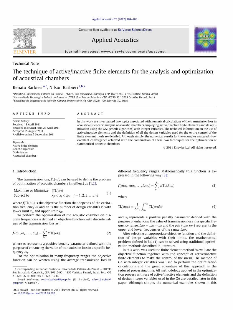
In this example it is shown the optimization of a single chamberwith extended inlet/outlet ducts. The single chamber has thefollowing geometric data: D = 150 mm for the chamber diameter,d1 = d2 = 50 mm for the inlet/outlet diameter ducts, andL = 300 mm for the chamber length.

With these geometric features and considering c = 346 m/s, thefirst two frequencies of this chamber with null acoustic attenua-tion are f1 = c/2L = 576.66 Hz and f2 = c/L = 1153.33 Hz. These val-ues for f1 and f2 also could be obtained with finite elements, as

h1 h2

300

25

50

Fig. 4. Finite element mesh and design variables (real).

0 500 1000 1500 2000 2500 3000

Frequency [Hz]

0

10

20

30

40

50

60

TL

Fig. 5. TL(x) for single chamber (dashed line) and for optimized chamber withextended inlet/outlet ducts (solid line).

186 R. Barbieri, N. Barbieri / Applied Acoustics 73 (2012) 184–189

can be seen in Fig. 5. Based on this information it selects two fre-quency ranges to maximize the TL(x) with the following objectivefunction:

f ðDx1;Dx2; . . . ;DxnÞ ¼Xn

i¼1

aiTLðDxiÞ

¼ 150

Z 600

550TLðxÞdxþ 1

100

�Z 1200

1100TLðxÞdx ð5Þ

where the integrals are numerically calculated with the Simpsonrule and TL(x) is evaluated with step of 5 Hz. In this way, are nec-essary 11 calculations of TL(x) to evaluate the first integral and 21calculations to evaluate the second integral.

In the evaluation of TL(x) is used the quadratic (9 nodes) finiteelement and the mesh illustrated in Fig. 4. Only two design

h1

(a) Design domain. (b) D

R

Fig. 6. Geometry, finite element

Fig. 7. Geometry and finite elem

variables (x1 and x2) are necessary to control the h1 and h2 lengthsof the inlet/outlet extended ducts. These design variables definesthe number of inactive elements of the finite element mesh whichappear filled with black color in this Fig. 4. Therefore, the limits forthese design variables (integers) defined for the solution of thisexample are 0 6 x1 6 30 and 0 6 x2 6 25, because the mesh ishomogeneous with element size of Dh = 5 mm. Although this is amesh with small number of elements the results can be consideredreliable until the frequency of 3000 Hz which is the upper valueshown in Fig. 5. The analysis of phase and amplitude errors(numerical � analytical) for linear acoustics problems is widelystudied in the literature [3,5]. The number of elements per wave-length at 3000 Hz calculated with the mesh shown in Fig. 4 isaround 23. Using this value and the results shown by Barbieriet al. [3] is expected errors in the order of 0.01% in wave amplitudeand 0.1% at phase for nearly singular problems (k-singularity). Forthe frequencies far from this kind of singularity the errors expectedfor the amplitude and phase are much lower, around 0.004% and0.01% respectively.

The design variables x1 and x2 are calculated as the integer partof h1/Dh and h2/Dh. Therefore, the maximum number of evaluationof the objective function to find the optimal solution to this finiteelement mesh is at most equal to 31 � 26 = 806. In relation tothe optimal values calculated with real variables it is expectedmaximum error in h1 and h2 of 2.5 mm which corresponds to halfthe characteristic size of the element.

The convergence is achieved in the first generation (iteration)with 25 evaluations of the objective function. Fig. 5 shows thetwo frequencies range used to define the optimization intervals(550–600 Hz and 1100–1200 Hz) and the TL(x) curves for the sin-gle chamber (h1 = h2 = 0) and to the optimized chamber using ex-tended inlet/outlet ducts (h1 = 40 mm and h2 = 60 mm). It can benoted that between 1100 and 1200 Hz there is a drop in the opti-mized TL(x) curve due to use of elements with size of 5 mm. Re-

h3h2/2

70

25

25

70

h2/2

esign variables and control of mesh.

mesh and design variables.

ent mesh after optimization.

0 500 1000 1500 2000 2500 3000

Frequency [Hz]

0

10

20

30

40

50

60

70

80

90

TL

Fig. 8. TL(x) for optimized chamber with inlet/outlet extended ducts (dashed line)and with mini-chambers in the input (solid line).

Generation

15

20

25

30

35

40

45

f

5 10 15 20

Fig. 11. Convergence analysis for example 3.

0 100 200 300 400 500 600 700 800 900 1000

Frequency [Hz]

0

10

20

30

40

50

60

70

TL

Fig. 12. TL(x) curve after optimization and frequency range used in the optimi-zation Process.

R. Barbieri, N. Barbieri / Applied Acoustics 73 (2012) 184–189 187

sults for this optimization problem using real variables can befound in [6] and show that these drops in TL(x) curve can be elim-inated by refining the mesh.

3.2. Example 2

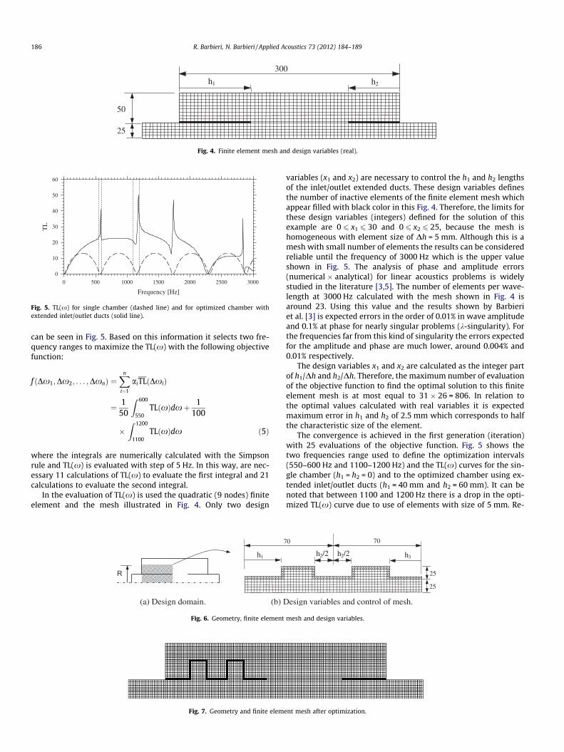
In the results shown in Fig. 5 is easily noted that the acousticattenuation in the frequency range from 2200 to 2400 Hz is lowerand a new optimization was performed in order to eliminate thisdisadvantage. The strategy employed was to use mini-chambersin the inlet duct in order to avoid significantly change in the vol-ume chamber and does not cause substantial changes in theTL(x) curve. Similar strategy was used by [7] who used corrugatedpipes to eliminate this kind of problem with satisfactory results.

In Fig. 6a is shows the design domain used to new optimizationproblem and Fig. 6b shows the design variables and the illustrationof a homogeneous mesh with Dx = Dy = 5 mm where the filled ele-ments represent the inactive elements.

The optimization process was carried out using homogeneousmesh with Dx = Dy = 2.5 mm and the geometric constraints im-posed to the design variables (integers) were defined as2 6 x1 6 16; 2 6 x2 6 16 and 2 6 x3 6 16. The frequency range usedto calculate the objective function was 2150 to 2450 Hz and the fi-nal geometry found is illustrated in Fig. 7 where the elements filledwith black color indicate the inactive elements (walls). The conver-gence to the optimum values was also achieved at the end of thefirst generation (25 iterations).

3

25

50

Fig. 9. Finite element mesh an

215

Fig. 10. Geometry and finite elem

The values found for the design variables were h1 = 32.5 mm;h2 = 25 mm and h3 = 30 mm with f = 44.806 dB. The TL(x) curveobtained with this new geometry is show in Fig. 8 and it can benoted significant increase of TL(x) in the frequency range of2000 to 3000 Hz and lower changes in other frequencies rangewere already expected in function of change in the in internal vol-ume of the chamber and the inlet/outlet ducts length.

0060 design variables

d design variables (real).

ent mesh after optimization.

h1

h2

300

25

50

h3

Fig. 13. Finite element mesh and design variables.

Fig. 14. Geometry and finite element mesh after optimization.

0 100 200 300 400 500 600 700 800 900 1000 1100 1200

Frequency [Hz]

0

20

40

60

80

100

TL

Fig. 15. TL(x) after optimization.

Fig. 16. Refining the local mesh to improve the accuracy of the results.

188 R. Barbieri, N. Barbieri / Applied Acoustics 73 (2012) 184–189

3.3. Example 3

In this example is show the optimization of the same simplecamera used in example 1, but the frequency range used in theoptimization was 350 Hz to 400 Hz and was defined 60 designvariables to define the design domain. Each of these design vari-ables takes the value 0 (inactive) or 1 (active). The inactive ele-ments indicate the existence of material (wall) and the activeelements indicate free passage of airflow. In Fig. 9 is illustratedthe situation where all elements of the design domain are inactive.

The optimization was performed using 25 evaluations of theobjective function for each generation and the objective functionwas calculated using Dx = 5 Hz and the same finite element meshof example 1. The optimum geometry obtained using these condi-tions is shown in Fig. 10 and it was reached after 8 generations

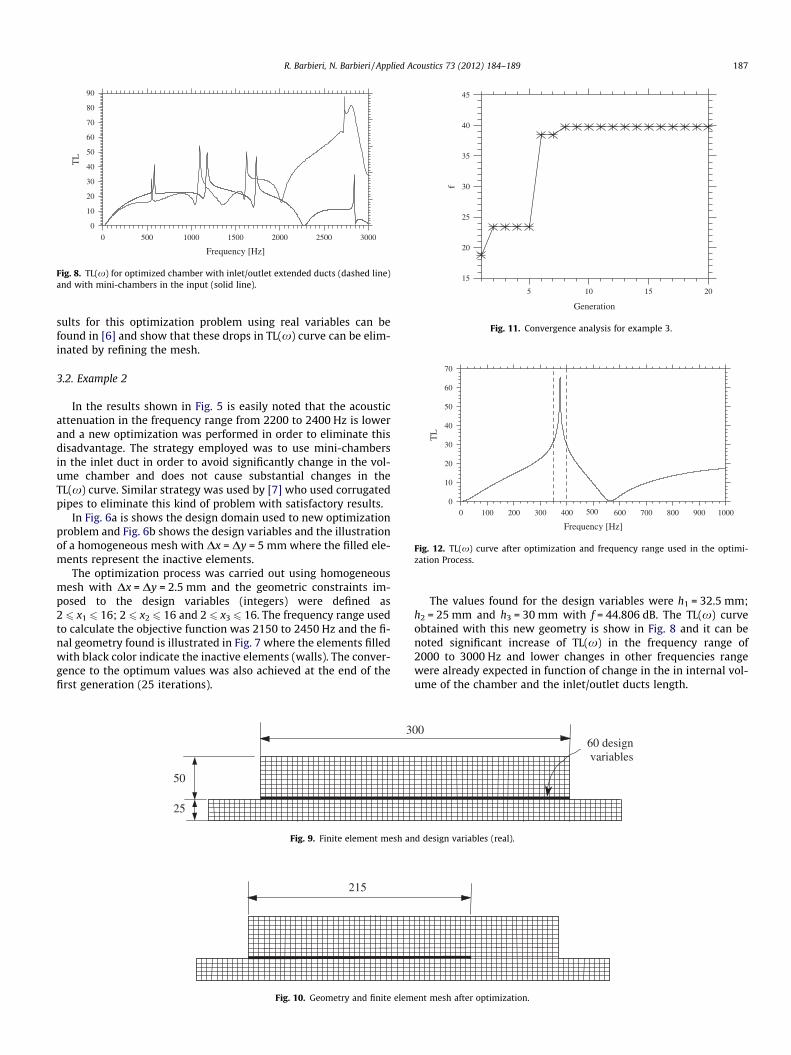
(200 evaluations of the objective function) as shown in Fig. 11.The TL(x) curve for these conditions is shown in Fig. 12 whichappears also marked the frequency range used in defining theobjective function.

3.4. Example 4

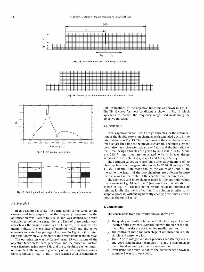
In this application are used 3 design variables for the optimiza-tion of the double extension chamber with extended ducts in theinternal division, Fig. 13. The dimensions of the chamber and cen-tral duct are the same as the previous example. The finite elementmesh also has a characteristic size of 5 mm and the limitation ofthe 3 real design variables are given by h1 6 160; h2 6 h1�5 andh3 6 295�h1 and they are associated with 3 integer designvariables: 1 6 x1 6 32; 1 6 x2 6 x1�1 and 1 6 x3 6 59�x1.

The optimum values were also found after 25 evaluations of theobjective function (one generation) with f = 47.36 dB and h1 = 150,h2 = h3 = 130 mm. Note that although the values of h2 and h3 arethe same, the length of the two chambers are different becausethere is a wall in the center of the chamber with 5 mm thick.

The geometry and finite element mesh for the optimum valuesthat shown in Fig. 14 and the TL(x) curve for this situation isshown in Fig. 15. Probably better results could be obtained byrefining locally the mesh after this first solution (similar to h-adaptive process) without significantly changing the finite elementmesh as shown in Fig. 16.

4. Conclusions

The conclusions from the results shown above are:

(1) The quality of results obtained with the technique of active/inactive finite elements is associated with the size of the ele-ment. Best results are obtained for smaller meshes.

(2) The control of mesh for each stage of optimization is quitesimple and extremely fast.

(3) The GA with integer variables produces satisfactory resultsand good convergence. Examples 1, 2 and 4 converged tothe optimal geometry in the first-generation.

(4) Even using 60 design variables the convergence shown inexample 3 was also very good.

R. Barbieri, N. Barbieri / Applied Acoustics 73 (2012) 184–189 189

References

[1] Luenberger DG. Linear and nonlinear programming. Addison-Wesley; 1989.[2] Bazaraa MS, Sherali HD, Shetti CM. Nonlinear programming. New York: Wiley;

1993.[3] Barbieri R, Barbieri N, Lima KF. Application of the Galerkin-FEM and the

improved four-pole parameters method to predict acoustic performance ofexpansion chambers. J Sound Vib 2004;276:1101–7.

[4] Lee JW, Kim YY. Topology optimization of muffler internal partitions forimproving acoustical attenuation performance. Int J Numer Meth Eng2009;80:455–77.

[5] Ihlenburg F, Babuska I, Sauter S. Reliability of finite element methods for thenumerical computation of waves. Adv Eng Soft 1997;28:417–24.

[6] Barbieri R, Barbieri N. Finite element acoustic simulation based shapeoptimization of a muffler. Appl Acoust 2006;67:346–57.

[7] Lima KF, Lenzi A, Barbieri R. The study of reactive silencers by shape andparametric optimization techniques. Appl Acoust 2011;72:142–50.