The Termination of Commercial Mortgage Contracts through...

2002 V30 4: pp. 595–633

REAL ESTATE

ECONOMICS

The Termination of Commercial MortgageContracts through Prepayment and Default:A Proportional Hazard Approach withCompeting RisksBrian A. Ciochetti,∗ Yongheng Deng,∗∗ Bin Gao∗∗∗ and Rui Yao∗∗∗∗

This article examines the factors driving the borrower’s decision to terminatecommercial mortgage contracts with the lender through either prepayment ordefault. Using loan-level data, we estimate prepayment and default functionsin a proportional hazard framework with competing risks, allowing us to ac-count for unobserved heterogeneity. Under a strict definition of mortgage de-fault, we do not find evidence to support the existence of unobserved hetero-geneity. However, when the definition of mortgage default is relaxed, we dofind some evidence of two distinctive borrower groups. Our results suggestthat the values of implicit put and call options drive default and prepaymentactions in a nonlinear and interactive fashion. Prepayment and default risksare found to be convex in the intrinsic value of call and put options, respec-tively. Consistent with the joint nature of the two underlying options, high valueof the put/call option is found to significantly reduce the call/put risk sincethe borrower forfeits both options by exercising one. Variables that proxy forcash flow and credit conditions as well as ex post bargaining powers are alsofound to have significant influence upon the borrower’s mortgage terminationdecision.

A better understanding of commercial mortgage termination through defaultor prepayment has important academic as well as practical implications. Withtheir relatively simple financial structure—one underlying property and onecollateralized debt obligation—commercial mortgages provide an ideal eco-nomic setting to test the rationality of investors and the empirical applicabilityof contingent claim models. From a practitioner’s perspective, the identifica-tion of factors relating to default and/or prepayment help efficiently deter-mine not only the appropriate spreads in the underwriting of whole loans, but

∗University of North Carolina–Chapel Hill, Chapel Hill, NC 27599 or [email protected].

∗∗University of Southern California, Los Angeles, CA 90089 or [email protected].

∗∗∗University of North Carolina–Chapel Hill, Chapel Hill, NC 27599 or [email protected].∗∗∗∗CUNY-Baruch College, NY, NY 10010 or rui [email protected].

596 Ciochetti et al.

also diversification strategies affecting pools of loans by such categories asproperty type and geographic location. For fixed income investors, an appropri-ately specified empirical termination model can provide a structured method-ology to incorporate contemporaneous information in the valuation of not onlywhole commercial loans, but also their securitized counterparts. Moreover, sucha model provides a basis for regulators to efficiently set standards in risk-basedminimum capital requirements for both life insurance companies as well ascommercial banks.

Despite the importance of the topic, there has been a dearth of empirical re-search on commercial mortgage termination, primarily due to the lack of datawith which to examine the asset class. Kau et al. (1990) provided a theoret-ical analysis of commercial mortgage valuation. On the empirical side, mostrelated studies have been conducted using aggregate levels of data (Titman andTorous 1989 and Elmer and Haidorfer 1997). Yet disaggregate loan historiesare needed to fully understand the relationship between loan characteristics andthe economics of commercial mortgage termination.

Limited studies using loan-level data have focused on one termination event,either default or prepayment. In one of the early efforts to explain borrowerbehavior, Vandell et al. (1993) study foreclosure experience of commercialmortgage loans and find that the equity position, as measured by the contem-poraneous market loan-to-value ratio (LTV), is highly significant in explainingmortgage default. However, short-term cash flow conditions, as proxied byoriginal debt service coverage ratio (DCR), are statistically insignificant in ex-plaining default risk. Property type is also found to affect default hazard rates.While this study enhances our understanding of the default experience, severalissues hamper interpretation of the results. First, default is construed as of thedate of loan foreclosure. Yet Brown, Ciochetti and Riddiough (2000) find thatthere is routinely a lag of 6 to 22 months between the start and completion of theforeclosure process. Use of completed foreclosure as the default event date maynot accurately measure the economic environment facing the borrower whenmaking a default decision. Second, the use of regional-level property indicesto update property values may not fully capture the variability in these values.By excluding property type, the measurement error in the aggregate indicesmay introduce noise, and the significance of property type dummies reportedby Vandell et al. (1993) may simply reflect the measurement error in propertyvalue, as opposed to the differential propensity of default on loans secured bydifferent types of property. Third, use of DCR at origination does not capturecontemporaneous cash flow conditions, perhaps explaining its lack of signifi-cance in affecting the default decision. Last, the study terminates in 1989, priorto the onset of the real estate recession of the early 1990s, thus failing to capturethe significant increase in credit-related mortgage default during this period.

Termination of Commercial Mortgage Contracts 597

In a recent study of multifamily mortgage default experience, Archer et al.(2000) identify the significance of original DCR but not original LTV. Us-ing a logit approach to modeling mortgage default, the authors argue thatLTV, DCR and mortgage rate spread are endogenously and simultaneouslydetermined during initial negotiations between equity and debtholders. The re-sulting multicolinearity makes it difficult to identify a significant correlationbetween these underwriting variables and the likelihood of default. One ex-planation for this insignificance may be due to the lack of contemporaneousupdating of variables. This may be important, since economic and financialconditions may have changed dramatically from loan origination to the defaultevent.

While important in advancing our understanding of commercial mortgage ter-mination, both studies fail to consider the impact of prepayment on the optionto default, yet default and prepayment are competing risks because the bor-rower forfeits one option through the exercise of the other. Empirical work oncommercial mortgages generally dismisses prepayment as a result of contract-ing issues. Many loans include some form of lockout, prepayment penalty, oryield maintenance provision. Yet these forms of contracting did not becomewidespread in the commercial mortgage markets until the mid- to late 1980s.Even with penalties, however, prepayment is found to occur frequently, result-ing in pricing fluctuations larger than those associated with default risk (see Fu,LaCour-Little and Vandell 2000).

Follain, Ondrich and Sinha (1997) estimate a prepayment function with a non-parametric baseline function and gamma-distributed heterogeneous errors usinga sample of Federal Home Loan Mortgage Corporation (FHLMC) multifamilyloans. The authors find that prepayment is sensitive to the value of the calloption, but the responsiveness is short of what one expects in the context of apure option-based pricing model. The study also identifies the importance ofunobserved heterogeneity in explaining multifamily prepayment experience,providing corroboration of prior research on residential loans (see Stanton1995).

Fu, LaCour-Little and Vandell (2000) examine the effectiveness of variousprepayment penalty structures embedded in multifamily commercial mort-gage contracts. The authors hypothesize that prepayment occurs either because(1) the assumed prepayment penalties do not exist, (2) the prepayment penal-ties are less severe than assumed, or (3) borrowers overexercise prepaymentirrationally from an option-theoretic perspective or incorporate factors beyondthose able to be incorporated in a generalized option-theoretic model of prepay-ment. A prepayment hazard model is specified and estimated using a sample ofmultifamily loans. The authors find that the nature and terms of the prepayment


penalty significantly affect the pattern of prepayment. Results of the study areconsistent with both theoretical and numerical predictions.1

A potential shortcoming of all the studies reviewed is the failure to model de-fault and prepayment events simultaneously and interactively in a competingrisk framework. Moreover, these studies do not consider the effects of con-temporaneous cash flow conditions on put and call risks. In a recent study ofthe behavior of single-family borrowers, Deng, Quigley and Van Order (2000)model default and prepayment as dependent competing risks to effectively ex-amine the joint nature of the put and call options. Strong support is found tosuggest that the value of the put(call) has a significant effect on the call(put)risk. The discrete specification of unobserved heterogeneity allows borrowersto be differentiated into groups based on relative riskiness. In terms of prepay-ment, the high-risk group is found to be approximately 3 times riskier thanthe intermediate group and 20 times riskier than the low risk group. For de-fault, however, borrowers are found to be rather homogeneous.2 The authorsattribute the significance of heterogeneity to either differences in borrowers’sophistication in exercising mortgage options or differences in levels of unob-served transaction costs. However, unobserved heterogeneity may also capturethe measurement errors in option values and observable transaction costs.3

In an earlier study, Deng, Quigley and Van Order (1996) analyze a sampleof low-down-payment residential mortgages that default in a competing riskframework, with a model that considers default and prepayment options asinterdependent competing risks. While these two studies are the first to exam-ine prepayment and default in a competing risk framework, their analysis isconducted on residential mortgage contracts. Commercial mortgages are verydifferent from their residential counterparts in that they are typically used tofinance investment properties with debt payments being made from cash flowsprovided by underlying lease contracts. Thus, the factors driving the mortgagetermination decision and the homogeneity/sophistication of commercial bor-rowers may be very different than in the residential mortgage markets.

1 See also Ambrose and Sanders (2001) and Goldberg and Capone (1998) for additionaldiscussion on commercial mortgage terminations.2 Defaults on residential mortgages are rare events because of incomplete separation ofinvestment and consumption decisions in housing as well as the high costs of default onpersonal credit.3 The put option is proxied by probability of negative equity, based on estimated stochas-tic processes of interest rates and property values. However, to a particular borrower theprobability of default is either one or zero, which implies the proxy is either underesti-mated (high risk group) or overestimated (low risk group). The original LTV, state-levelunemployment rates and divorce rates may also be noisy measures of contemporaneoustransaction costs at the individual borrower level.


In this study, we investigate a portfolio of 2,090 commercial mortgages orig-inated by a major life insurance company over the period 1974 through 1990and tracked through year-end 1995. We examine the following issues associatedwith commercial mortgage default and prepayment:

1. To what extent do put and call options explain the default and prepay-ment decisions of commercial mortgage borrowers?

2. How important are modeling default and prepayment risks simultane-ously as dependent competing risks?

3. How essential are transaction costs and unobservable heterogeneityamong commercial mortgage borrowers in affecting the terminationof mortgage debt?

4. To what degree does the definition of mortgage default impact observedbehavior by mortgage borrowers?

Our findings suggest:

1. Put and call options are highly significant in explaining commercialmortgage default and prepayment. Ceteris paribus, the more in-the-money the put (call) option is, the more likely the mortgagor will default(prepay). Moreover, the effect of the intrinsic value of the put and calloptions on the default and prepayment hazard is nonlinear and convex,a finding consistent with option pricing theory.

2. Borrowers forfeit both options by exercising either. Consistent withthe joint nature of the options, we find that high values of put optionsincrease the value of delay in the exercise of the call option, hencereducing prepayment risk, and vice versa.

3. Transaction costs are important supplements to the option variablesin explaining mortgage termination. Specifically, there are significantcash flow, credit and size effects. Enhanced solvency conditions reducedefault risk, but they increase the likelihood of prepayment. Low equitylevels significantly reduce the possibility of prepayment. Relative totheir larger counterparts, borrowers of small loans default much lessfrequently but prepay more often.

4. Under a strict definition of mortgage default, we do not find evidenceof heterogeneity among borrowers. However, when the definition ofmortgage default is relaxed, we do find some evidence of heterogeneityin borrower behavior.

The remainder of the article is organized as follows. The next section de-scribes the characteristics of commercial mortgage markets and derives optimal


exercise conditions for mortgage options in the presence of cash flow, creditconstraints and contracting costs. The third section introduces a proportionalhazard model with competing risks and unobserved heterogeneity. In the fourthsection, we describe the data and summary statistics. In the fifth section wepresent results of our empirical estimations. Discussion about the robustness ofour findings follows in the sixth section. Implications and concluding remarksare provided in the seventh section.

Characteristics of Commercial Mortgage Termination

In this section, we first describe the features of commercial mortgage contracts,followed by derivation of sufficient conditions for borrowers to exercise mort-gage options in a frictionless world. We then discuss the effects of transactioncosts on prepayment and default, which include cash flow or credit constraintsand incomplete contracting.

Characteristics of Commercial Mortgages

Commercial mortgage markets differ from their residential counterparts in sev-eral significant respects. Commercial loans finance investment opportunitiesand are typically used by sophisticated investors and real estate developers.Thus, borrowers of commercial debt have very low “psychological” attach-ment to the underlying asset and should, in theory, be more “ruthless” in theexercise of either the default or prepayment option. Loans are typically fixed-rate and fixed-payment notes without recourse and are either interest-only oramortizing, with a balloon payment prior to the full amortization term.

Embedded in each mortgage is a termination option that can be exercised by theborrower through either default or prepayment. If the borrower chooses to foregoscheduled payments for (up to) 90 days, a foreclosure process typically ensues.Two outcomes are possible. The lender can choose to foreclose and directlyown the property or, alternatively, renegotiate the debt contract, often deferringor accepting less than full payment. The borrower can also end the contractingrelationship with the lender by prepaying the outstanding loan balance, subjectto any applicable prepayment penalties.4

4 After the mass prepayment wave in the late 1970s and the early 1980s, banks andlife insurance companies began to implement various protective covenants in mortgagecontracts to stabilize expected cash flows through a reduction in prepayment incentives.These included lockout periods, prepayment penalties and yield maintenance provisions.The most severe of these is the yield maintenance provision, under which the borroweris required to pay the full difference between the accounting mortgage balance and themarket value of the mortgage. This, at least in theory, would fully eliminate any pre-payment incentives from the borrower’s perspective (see Fu, LaCour-Little and Vandell2000).


Optimal Decision Rules without Transaction Costs

In the context of corporate finance and contingent claims literature, borrowersmay be viewed as equityholders and lenders as debtholders. It is well knownthat the equityholder faces an optionlike payoff. With limited responsibility, theequityholder can default on the debt and return the asset to the debtholder. Thepossibility of prepaying the debt gives the mortgage borrower another valuablefinancial advantage. Let us define “termination option” as the value of the op-portunity for the equityholder to terminate the debt contract with the debtholderthrough default or prepayment. Under prepayment, the borrower “repurchases”the remaining mortgage obligation at the current loan balance, plus any appli-cable prepayment penalties. Under a default scenario, the borrower “sells” theproperty to the lender at a price equal to the market value of mortgage. Thisreflects the opportunity cost of the future scheduled mortgage payments to theborrower. At any time, the choice to exercise a termination option will be donethrough the vehicle (put or call) with the largest intrinsic value, causing bothfuture choices to be lost immediately. The borrower can, however, choose tokeep the option alive by paying the current period scheduled payment. Thus, inthe absence of transaction costs, the borrower will exercise the option at time tif the following condition is satisfied before he submits the periodic principaland interest payment:

max{Lt − Vt ; Lt − Bt − ft .; 0} ≥ Et

[Pt+1

1 + r f

]− Dt , (1)

where Vt is the property value at time t and Lt is the market value of the debt. Lt

can be expressed as the sum of remaining mortgage payments discounted at theprevailing market mortgage rate, Mt. Bt is the accounting outstanding balance ofthe debt, which equals the sum of remaining mortgage payments discounted atthe contract rate, Rc. ft is the prepayment penalty as specified in the contracts.5

Thus (Lt − Vt) defines the intrinsic value of the put option, while (Lt − Bt −ft) defines the intrinsic call value to the borrower at time t. The left-hand side(LHS) of Inequality (1) defines the payoff of the termination option if exercisedat time t. On the right-hand side (RHS), Pt+1 is the value of the terminationoption that is (at least) a function of Vt+1, Lt+1, Bt+1, Mt+1 and Rc. Dt is thescheduled payment at time t.6 rf is the risk-free rate between t and t + 1, andEt[Pt+1/(1 + rf )] defines the expected (discounted) value of the option in thesubsequent period if not exercised today. Expectation on Pt+1 is taken overall possible realizations of property value Vt+1 and mortgage rate Mt+1, whichrelate to Vt and Lt, respectively, through property value and mortgage rate

5 ft can be set as infinity in the case of lockout period.6 For step and graduated payment loans, Dt is time dependent.


processes. Standard option pricing theory suggests that Pt, as the option value,should be convex in its intrinsic value (see Merton 1973). Also, as the optionapproaches expiration date—in the case of a balloon mortgage, rollover, orextension date—its exercise boundary will be closer to the option’s strike price.In sum, Inequality (1) suggests that borrowers should exercise the terminationoption if it is sufficiently in the money—if the intrinsic option value today plusthe saved cash payment is greater or equal to the discounted option value in thenext period—otherwise it is optimal to tender the scheduled payment and keepthe option alive for at least one more period.

Optimal Decision Rules with Transaction Costs

Although contingent claim theory calls for a sharp exercise boundary, empiri-cal evidence in the mortgage literature seems to contradict this theory. Ratherthan appealing to investors’ irrationality, researchers have recognized that un-observed, heterogeneous transaction costs may offer a valid explanation to theblurred exercise boundary (see Deng, Quigley and Van Order 2000). Such costsmay arise from liquidity or credit constraints, incomplete contracting and/orborrower risk aversion, all of which vary from borrower to borrower.

Cash Flow and Credit Effect

In the absence of transaction costs, it is not optimal for a cash-flow-constrainedborrower to default with positive equity in the property since additional eq-uity financing could be secured to alleviate cash-flow constraints. But in morerealistic settings, additional borrowing can be quite costly, especially for bor-rowers with liquidity constraints, since a low DCR will most likely disqualifyborrowers from typical market-rate financing. An alternative solution for cash-constrained borrowers is to sell the property and pay off the debt at its facevalue. However, selling per se can also be costly for borrowers in financialdistress.7

Default can also lead to a lower credit rating or higher costs of financ-ing subsequent projects. This cost can be especially large for new and/orsmall investors in the commercial real estate business. While more establishedborrowers/developers might convince lenders that general market conditionscause default, an inexperienced investor in the business is more likely to be ac-cused of poor management of the property and held responsible for its default.In addition, smaller investors might sell their property and prepay their loans

7 Pulvino (1998) shows that financially constrained airlines receive lower prices thantheir unconstrained rivals when selling used narrow-body aircraft.


out of consumption-related reasons since they are more likely to be liquidityconstrained.

Credit and liquidity levels also impact exercise of the call option by affectingavailable refinancing rates. A borrower with good credit can qualify for betterterms in a falling-interest-rate environment, which further raises the opportunitycost of maintaining the current mortgage and hence the attractiveness of theprepayment option. On the other hand, institutional requirements for reasonableLTV and DCR levels can disqualify many borrowers from favorable marketrates. Facing higher borrowing costs for personal consumption or businessexpansion, a small investor may sell the property or prepay a mortgage even ina rising interest rate environment to “cash out” equity.

Contract Incompleteness

Borrowers with negative equity positions are frequently observed not to exercisethe default option, particularly when the net operating income (NOI) is sufficientto cover scheduled debt payments. Instead of handing over the property to thedebtholder, they try to extract as much value as possible from the property,typically through underinvestment. Since the property will most likely go to thelender at maturity, further sabotaging of the condition of the property can onlymake the borrower’s equity position more negative. Therefore, the optionlikepayoff to the equityholder makes it optimal for the borrower to delay defaultat the expense of the lender.8 It is unclear what effect a balloon structure willhave on this moral hazard problem. The borrower has incentives to maintainthe property in anticipation of a negotiated settlement in situations where theborrower is unable to pay off the loan at the scheduled balloon date (see Tu andEppli 2002). Alternatively, since the balloon structure effectively shortens thematurity of the put option, there is more incentive for the borrower to underinvestin the property.

The “waiting-to-default” scenario described above is suboptimal from a so-cial welfare perspective, since underinvestment can damage the property to theextent that it costs the debtholder much more to repair after taking over theproperty. This creates a positive deadweight loss (see Jensen and Meckling1976). The debtholder will charge a premium, ex ante, to account for the “steal-ing behavior” of certain borrowers, leading to only a second-best contract. Ifcontracting is costless and complete, the debtholder can correct the subopti-mal behavior of the borrower by imposing provisions in the debt contract that

8 This is similar to the underinvestment problem for financially distressed firms withdebt “overhang” as discussed in the corporate finance literature (see Myers 1977).


specifically mandate borrowers to meet required maintenance levels. However,these contracts are costly to monitor and enforce ex post.9

In a frictionless world (i.e., without transaction cost), a rational borrower whohas both negative equity (LTV > 1.0) and low cash flow (DCR < 1.0) willcertainly become delinquent on debt payments to maximize his or her financialwelfare (see Vandell et al. 1993). Realistically, there is no costless delinquencyor bankruptcy for the borrower or the lender. Therefore, a straight bankruptcydecision (foreclosure) is often Pareto-dominated by ex post renegotiation andworkout. Debtholders are usually not as knowledgeable about the value of theproperty as the equityholder and not as skillful as the borrowers at managementof the property. Thus, they may be willing to restructure the debt and reduce theloan balance rather then foreclose the loan at the first sign of financial distress.A borrower with, or who is believed to have, more ex post bargaining power willhave higher incentive to default ex ante if he or she can convince the debtholderthat financial distress is caused by macroeconomic market conditions, ratherthan inappropriate management. This may result in an agreement to modifyand restructure the debt contract (see Riddiough and Wyatt 1994). A smallerinvestor without established history, however, will have more trouble conveyingthe same argument, often resulting in an immediate full foreclosure.10 We shouldnote that ex ante, the debtholder would charge a higher coupon rate to accountfor the ex post renegotiation, unless he or she can commit himself or herself toforeclosure to deter defaults ex ante.

Empirically, incomplete contracting is also observed for prepayment penalties.Borrowers have been observed to default “strategically” to prepay the mortgagewithout being subject to full yield maintenance penalties. Under a strategic de-fault scenario, borrowers sell the property and repay the loan to realize propertyvalue appreciation or a favorable interest rate environment in which to refinance.Lenders, fearing the lengthy legal process and losses associated with the fore-closure process, may accept less than the full difference in yields. The exactpenalty under this scenario is related to the lender’s ability to identify the valueof the property precisely as well as the relative bargaining power of the twoparties engaged in the strategic default game (see Riddiough and Wyatt 1994).

9 The problem posed here is a typical moral hazard problem, similar to that found in theinsurance market, where the owner of the property becomes careless once the insurancecoverage is contracted and the premium paid.10 This argument is consistent with Brown, Ciochetti and Riddiough (2000), who findthat among loans in delinquency, large ones are more likely to be restructured while smallones are more likely to be foreclosed. They also find that large loans take the lenderlonger to dispose of because of larger liquidity pressure, which potentially explains thereluctance of lenders to foreclose on large loans.


A Proportional Hazard Model with CompetingRisks and Heterogeneous Error

The application of a proportional hazard approach to modeling commercialmortgages is appropriate because of its efficiency in modeling the complete pathleading to mortgage termination events. Recent applications include Vandellet al. (1993), Deng, Quigley and Van Order (1996), Follain, Ondrich and Sinha(1997) and Pavlov (2001). The model we estimate in this study is based on theeconometric specification as used in Deng, Quigley and Van Order (2000).

Proportional Hazard Model for Single Risk

Assuming the probability density function of duration of the loan to first default(prepayment) at t is f (t) and the cumulative probability distribution is F(t), thehazard function is defined as the probability density of default (prepayment)between time t and t + �, conditional on its being active up to time t:

H (t) = lim�→0

Pr(t < T < t + � | T ≥ t)

�= f (t)

1 − F(t). (2)

Following the proportional hazard assumption of Cox (1972), we assume avector of covariates (or regressors), xi,t, either time invariant or time varying,that change the baseline hazard function, H0(t), proportionally in exponentialform. Thus the hazard function for subject i at time t can be specified as:

Hi,t (xi,t ; β) = H0(ti ) exp(x ′i,tβ), (3)

where β is the vector of constant coefficients. The convenient exponential spec-ification ensures that the hazard rate under different values of covariates isalways positive. Theoretically, the hazard function is continuous and can takeany nonnegative functional form. This flexibility, however, makes the empiricalidentification and estimation of the model a nontrivial exercise.

Several approaches to estimation have been developed in the literature. Thesimplest parametric specification assumes a given functional form (typicallyExponential, Logistic, or Weibull) and estimates the one or two unknownfunctional parameters. However, this choice inevitably exerts constraints onthe shape of the underlying hazard function, which can result in inconsisten-cies such as those shown in economic theory.11 A popular alternative is Cox’sPartial Likelihood (CPL) specification (see Cox 1975 as well as Cox and Oakes

11 An example in labor economics are the spikes in reemployment hazard at 26–27 weeksand 52–53 weeks, which correspond to the termination of unemployment benefits (seeKiefer 1988).


1984), which only requires the existence of a common stationary baseline haz-ard function, H0, for all subjects. The likelihood function under this scenariois decomposed into two separate parts, each containing unknowns in either thebaseline hazard function or the partial likelihood of the proportional changes.So, β can be identified without parametric restrictions on the baseline functionsince H0(t) factors out as a nuisance number. In this sense, the proportionalhazard model is semiparametric: nonparametric in the baseline hazard func-tions and parametric in the specifications of proportional change. However,in economic research, the shapes of baseline hazard are often of great interestthemselves, and Cox’s specification poses an inconvenience in those cases. Sug-gested remedies include a two-step procedure where regression coefficients, β,are first identified through Cox Partial Likelihood estimation. These coefficientsare then employed in the full likelihood estimation to obtain the necessary pa-rameters for a flexibly specified baseline hazard function, typically a high-orderpolynomial function of time.12

A full parametric likelihood function with continuously changing baseline haz-ard rates is computationally difficult to converge. A tractable solution is tospecify a fully parametric likelihood function with a discrete flexible base-line hazard function and estimate the parameters of proportional hazard effectand baseline hazard functions simultaneously (see Han and Hausman 1990,Sueyoshi 1992, and Deng, Quigley and Van Order 2000 for examples).13

Discrete Proportional Hazard Model with Competing Risksand Unobserved Heterogeneity

Modeling both default and prepayment of commercial mortgage debt as com-peting risks is a natural choice, as borrowers forfeit both the future option todefault and the future option to prepay by exercising either. The discrete com-peting risk proportional hazard function for observation i at time t can be definedas:

H di,t (xi,t ; βd ) = exp

(γ d (t) + x ′

i,tβd)

(4)

H pi,t (xi,t ; βp) = exp

(γ p(t) + x ′

i,tβp)

(5)

for default risk and prepayment risk, respectively, where γ κ (t) is the log ofintegrated baseline hazard rate for risk type k between t − 1 and t.

12 See Fu, LaCour-Little and Vandell (2000) for an application of this approach.13 Discrete in the sense that the hazard is a step function that takes constant valuesbetween time t and t + 1.


Let td and tp be the duration of a mortgage until it is terminated by default orprepayment, respectively. The joint survival function can then be defined as14

S(td , tp | X, θd , θp) = exp

(−θd

td∑t=1

exp(γ d (t) + x ′

t βd

)

− θp

tp∑t=1

exp(γ p(t) + x ′

t βp

))(6)

where (θd , θp) are unobservable heterogeneity (location) parameters, which cancapture differences in unobserved transaction cost structures among borrowersafter controlling for observable heterogeneity. For example, some mortgagorsmay be more financially sophisticated and sensitive to refinancing and defaultrisks or have an unusually good or bad credit history. In a general specifica-tion, (θd , θp) are J pairs of distinct, but unobserved, types of individuals in thepopulation, each occurring with relative frequency pj, j = 1, 2, . . . , J. However,to avoid overparameterization, we limit ourselves to two groups in this study(J = 2).

The competing risk nature of mortgage options makes only the first realized ter-mination (default, prepayment, or censoring) observable, that is, t = min(td, tp,

tc). Define Fd(k | θd , θp) as the probability of mortgage termination by defaultin period k, Fp(k | θd , θp) as the probability of mortgage termination by prepay-ment in period k and Fc(k | θd , θp) as the probability that the mortgage survivesuntil period k.15 Following McCall (1996), we can write the probabilities as16

Fd (k | θd , θp) = S(k, k | θd , θp) − S(k + 1, k | θd , θp) − 0.5{S(k, k | θd , θp)

+ S(k + 1, k + 1 | θd , θp) − S(k, k + 1 | θd , θp)

− S(k + 1, k | θd , θp)}, (7)

Fp(k | θd , θp) = S(k, k | θd , θp) − S(k, k + 1 | θd , θp) − 0.5{S(k, k | θd , θp)

+ S(k + 1, k + 1 | θd , θp) − S(k, k + 1 | θd , θp)

− S(k + 1, k | θd , θp)}, (8)

14 We drop the index i for notation simplicity.15 In the estimation of the competing risk hazard model, censored observations includeall matured loans and active loans as of the end of the study period.16 The terms 0.5{· · ·} in Equations 7 and 8 are adjustments for discrete time specificationof duration dependence.


Fc(k | θd , θp) = S(k, k | θd , θp). (9)

The unconditional probability is then given by

Fm(k) =J∑

j=1

p j Fm(k | θd j , θpj ), m = p, d, c; (10)

and the log likelihood function of the fully specified competing risk proportionalhazard model with unobserved heterogeneity is given by

log(L)=N∑

i=1

{Iid log(Fid (ki )) + Iip log(Fip(ki )) + Iic log(Fic(ki ))}, (11)

with N being the total number of observations and Iid, Iip and Iic being theindicator functions that take values of one if the ith loan is terminated by de-fault, prepayment, or censoring, respectively, and zero otherwise. Neglectingheterogeneity leads to biased β estimates (toward zero), which may impact thestatistical inference. Specification with heterogeneity also allows for an exami-nation of the correlation between two exercise choices. For instance, a borrowermay be sophisticated in the decision to exercise one option, but insensitive withthe other—negative correlation—or unsophisticated at both, which implies apositive correlation between the propensity to prepay and default.

Empirical Analysis

In this section, we first discuss the source of data used in the study and the con-struction of empirical variables, followed by a discussion of summary statistics.

Sources of Data and Construction of Variables

The data used in the study come from several sources. Loan-level data aresecured from a large, multiline life insurance company and consist of 2,589individual loans originated over the period 1974 through 1990. Relevant loan-level characteristics include loan size, contract interest rate, loan term, quarterlystatus indicator, contractual payment information, borrower type, property typecollateralizing the loan, and geographic location.17 Property value and cashflow indices are secured from the National Council of Real Estate InvestmentFiduciaries (NCREIF), and data from the American Council of Life Insurance(ACLI) are used to provide a proxy for prevailing commercial mortgage interestrates.

17 Loans are categorized on a quarterly basis as active, 30 days delinquent, 60 daysdelinquent, 90 days delinquent, restructured, in process of foreclosure, foreclosed, paidin full, or prepaid.


Empirical analysis requires contemporaneous information regarding property(asset) values, property cash flow levels (net operating income) and mort-gage debt values. Since these are not observable directly, we use the quar-terly NCREIF property and income return series, stratified by eight geographicregions and four property types, to approximate the price paths of individ-ual properties.18 We then match estimated property values with the NCREIFincome return index as stratified by property type and region to construct a con-temporaneous net operating income (NOI) series.19 Using this methodology,we are able to match 2,090 individual loans with the NCREIF series. ACLIcommitment rate data are used to provide an estimate of the contemporaneousmarket value of each mortgage from the borrower’s perspective. We do so byfitting a third-order polynomial function to the quarterly ACLI commitmentseries, using the remaining loan term to account for the term structure effectassociated with each mortgage. Separately, we calculate the spread between thequarterly mean commitment rate, by property type, and the mean commitmentfor all mortgage commitments in that quarter. This spread is then added to thefitted mortgage rate to create a contemporaneous mortgage contract rate. Con-temporaneous market loan values are estimated as the sum of the remainingcontractual payments, discounted at the appropriate rate as described above.20

We measure the extent to which the put option is in the money with the contem-poraneous “LTV RATIO,” computed as the ratio of the market value of the loanto the market value of the property. As discussed in Section 2, since (Lt − Vt)is the exercise value of the put option, we can view LTV RATIO as one plus thescaled (by property size) intrinsic value of the put.21 LTV RATIO also affectsprepayment decisions. From a pure option perspective, a high value (greaterlikelihood) of prepayment in the future will give the borrower more incentive tokeep the mortgage termination option alive. From an institutional perspective,

18 For years between 1974 and 1978 where NCREIF data are not available, the Marshalland Swift construction cost index is used to supplement the NCREIF property valueindex.19 The index as stratified by region and property type is not complete since it is notavailable for some years and for some regions. In those cases, a more aggregate indexis used. For the index to be useful, we impose the condition that it must have at least36 quarters of data (or nine years) at the region and property level, in to capture thetremendous property value fluctuation in the early 1990s.20 Deng (1997) argues for the superiority of using the stochastic term structure model tocalculate the value of the loan numerically. But that methodology will require the choiceof (1) an appropriate term structure model and (2) a set of parameters for the specifiedprocess. The method used in the present study has the advantages of parsimony andcomputational efficiency.21 The constant term, one, is absorbed by the baseline hazard function, and will thus notaffect the estimates of the coefficients.


the LTV RATIO can affect the refinancing decision; a high LTV RATIO (lowequity level) will make it more difficult for the borrower to secure alternativefinancing, thus reducing the prepayment hazard. The LTV RATIO is also a mea-sure of financial leverage. Commercial mortgage borrowers with a low ratio areobserved to rationally refinance to lever up his or her equity in the property torealize tax benefits and/or enhance investment returns. Borrowers may also beexpected to prepay or sell properties with a low LTV RATIO in order to “cashout” their equity positions either for personal consumption or business expan-sion. This may occur even in the absence of contemporaneous market interestrate benefits.

The financial incentive to prepay is measured by the contemporaneous “CALRATIO,” estimated as the ratio of the outstanding loan balance less the marketvalue of the loan to the market value of the loan. Thus, the CAL RATIO is thescaled intrinsic value of prepayment for the borrower. We expect CAL RATIO toreduce the default hazard in the context of a joint mortgage option. The effect,however, may be rather small since refinancing will be very unlikely when aproperty is close to default. Conversely, the coefficient on CAL RATIO could bepositive in a “strategic default” scenario, one in which a borrower intentionallydefaults to trigger an acceleration of the loan to avoid a prepayment penalty ina favorable interest rate environment.

To capture the convexity of the option value with respect to its intrinsic value,we also include squared terms for LTV RATIO and CAL RATIO. These termsare denoted as “LTV SQUARED” and “CAL SQUARED.”

Short-term solvency status of the equityholder is measured by contemporane-ous “DCR,” estimated as the ratio of contemporaneous NOI to scheduled debtservice payments. Insufficient cash flow can result in default if additional equityborrowing is unavailable or becomes too expensive. Low DCR is also likelyto diminish the prepayment hazard, as insufficient cash flow disqualifies bor-rowers from refinancing at market rates. We note that NOI is constructed fromcontemporaneous property value and income return indices, thus not relyingon the DCR at loan origination, which may contain more idiosyncratic infor-mation about the cash flow conditions of the property at loan origination. DCRat loan origination, however, is included in the hazard regression, denoted as“ORIGDSC.”

With the financial incentive associated with option exercise measured in rel-ative form by LTV RATIO and CAL RATIO, a loan size variable is neededto capture the quantitative difference of the option value. If there is a fixedcost associated with option exercise, then larger loans should be associatedwith a higher likelihood of exercise for both the put and call options. To


capture this effect, we include in our regression loan size dummies, SMALL,MEDIUM and LARGE.22 To proxy for management expertise, financial sophis-tication, borrowing costs, and ex post bargaining power, we also include a set ofborrower type dummies, INDIVIDUAL, PARTNERSHIP, CORPORATION andOTHER.

Loan type dummies, AMZDUMMY for amortized loans, ACRDUMMY for ac-crual loans, GPMDUMMY for loans with changeable payments or step pay-ments and FIXED for fixed rate loans are also included. These variables capturethe variation in required periodic payment, which is the cost associated withkeeping the mortgage termination option alive. Accrual and step-rate loans ex-hibit increasing periodic payments, hence a greater likelihood of option exerciseover time. Loan-type dummies also reflect differential debt-equity structures atthe balloon payment. Relative to interest-only loans, those with amortizationprovisions have less principal due at maturity and hence larger equity posi-tion. We expect amortizing loans to have a lower probability of default at loanmaturity.

Property type dummies, APARTMENT, OFFICE, INDUSTRIAL, or RETAILare also included to capture property-related cash flow and risk characteristics.Property type has been shown to be significant in explaining commercial mort-gage default hazard rates in prior studies (see Vandell et al. 1993). We alsoinclude region dummies, EN, ME, SE, SW, WM, WN, WP and NE.23 However,with a properly specified model, and under rational borrower decision making,we would not expect to find either property type or region to be significant inexplaining termination of commercial mortgage contracts.

We also include a balloon dummy which takes the value of one if the loanis within one quarter of maturity date, zero otherwise. A risk-averse investorwith positive equity will be searching for alternative financing prior to thematurity date to avoid unintended de facto default with positive equity. Thosewith negative equity are not able to pay the loan in full at the balloon date,making default the optimal decision to exercise. From an option perspective,as the contract approaches maturity, the time value of the option is very smallrelative to its intrinsic value, encouraging borrowers to exercise the option andpocket the intrinsic value.

22 Loans less than $2 million in size are categorized as small, those greater than$2 million and less than $7 million are categorized as medium, and those greater than$7 million are categorized as large.23 These correspond to East North Central, Mideast, Southeast, Southwest, Mountain,West North Central, Pacific and Northeast regions, respectively.


Summary Statistics

As shown on Panel A of Table 1, the mean LTV at origination is slightly greaterthan 72%, and the corresponding debt coverage ratio averages 1.25. The aver-age maturity of loans in the sample is shown to be slightly less than 12 years.Loans are diversified across geographic regions, with greater concentrations inthe East North Central and Southeast regions of the country (Table 1, Panel B).Of interest is the incidence of default and prepayment as stratified by region ofloan origin. Loans originated in the Southwest region of the country exhibit notonly the greatest proportion of defaults, at 59%, but also the lowest prepaymentrate, at slightly greater than 12%.24 When stratified by property type securingthe loan, office properties are shown to dominate the sample, constituting nearly44% of the pool (Table 1, Panel C). There are more cases of default for officeproperties and more cases of prepayment among industrial properties. In termsof loan origination, a bimodal distribution is evident, with high loan activity inthe late 1970s and again during the mid-1980s (Table 1, Panel D). Loans ini-tiated in the mid-1970s and early 1980s have experienced greater prepayment,while loans originated in the early 1980s have experienced greater levels of de-fault. Overall, among the 2,090 loans employed in the study, slightly less than29% are shown to have prepaid and 27% are shown to have defaulted. Panel E ofTable 1 shows the distribution of the sample as stratified by loan size at orig-ination. Notice that borrowers of small loans have a propensity to default lessthan their larger counterparts, while large loan borrowers are shown to prepayless.

Over the period under examination, 1974 through 1995, tremendous fluctuationsin the value of commercial real estate property are found to have occurred(Figures 1 and 2), especially during the real estate recession of the late 1980sand early 1990s. The variation in property value assures a rather powerful testof the effect of option theory on mortgage termination. The sample’s meanmortgage coupon rate tracks that of the industry quite well, as proxied byACLI commitment rates, except during a brief period in the early 1980s, wheninterest rates and volatility were very high (Figure 3). Mean coupon rates forthe sample were approximately 100 basis points lower during this period thanthat as reported by ACLI (Panel D of Table 1 as well as Figure 3).

Loans that eventually terminate through default are shown to have a slightlyhigher initial LTV and slightly lower initial DCR (Table 2). The value of the calloption around origination is higher for loans that eventually default, suggest-ing that these loans may have been assessed a higher coupon rate premia up front

24 For purposes of describing the data, our definition of default includes all loans whichare in process of foreclosure, foreclosed, or modified.


Table 1 � Descriptive statistics.

Panel A: Means and standard deviations

Mean Std. Dev.

Origination year 1981.6 4.2Loan term (years) 11.9 5.4Coupon rate (%) 10.5 1.6Original DCR 1.25 0.18Original LTV (%) 72.2 6.2Loan size (MM) $6.7 $15.3

Panel B: Distributions by region

Number Percentage PercentageRegion of Loans Percent Default Prepaid

EN 396 18.9 17.4 35.1ME 201 9.6 25.9 25.4NE 222 10.6 37.8 22.5SE 267 12.8 28.1 23.6SW 157 7.5 59.2 12.1WM 222 10.6 39.6 26.1WN 99 4.7 32.3 33.3WP 526 25.2 13.5 35.7

Total 2,090 100.0 27.0 28.8

Panel C: Distributions by property types

Borrower Number Percentage Percentage PercentageType of Loans of the Total Default Prepaid

APARTMENT 420 20.1 23.8 28.1INDUSTRIAL 437 20.9 16.5 38.7OFFICE 914 43.7 35.6 24.1RETAIL 319 15.3 21.0 29.5

Total 2,090 100.0 27.0 28.8

Panel D: Distributions by origination years

Percentage of Mean Percentage PercentageYear # of Obs. the Sample Coupon Rate Default Prepaid

1974 61 2.9 8.75 4.9 40.11975 60 2.9 9.56 13.3 33.31976 86 4.1 9.71 16.3 51.21977 198 9.5 9.39 7.1 48.51978 232 11.1 9.49 9.1 29.71979 201 9.6 9.84 14.9 28.91980 160 7.7 10.56 17.5 23.1


Table 1 � continued

Percentage of Mean Percentage PercentageYear # of Obs. the Sample Coupon Rate Default Prepaid

1981 86 4.1 11.85 12.8 52.31982 53 2.5 14.64 13.2 73.61983 181 8.7 12.35 25.4 38.11984 117 5.6 12.79 47.0 15.41985 194 9.3 11.88 56.7 13.41986 152 7.3 9.95 52.6 15.81987 141 6.7 9.50 52.5 9.91988 94 4.5 9.67 45.7 13.81989 35 1.7 9.45 37.1 2.91990 39 1.9 9.42 18.0 7.7

Total 2,090 100.0 10.5 27.0 28.8

Panel E: Distributions by size

Loan Number Percentage Percentage PercentageSize of Loans of the Total Default Prepaid

Small (<$2M) 814 39.7 10.4 41.8Medium ($2–$7M) 721 35.1 27.6 26.4Large (>$7M) 517 25.2 48.2 3.4

Total 2,052 100.0 26.0 29.2

Note: Mean and standard deviation in Panel A are calculated based on 2,090 loans.

to negate the risk. At the time of termination, default/prepaid loans have muchlower/higher DCR ratios than active or matured loans and much higher/lowerLTV ratios. In general we find the data to be representative of the commercialmortgage universe over the period under examination.25

Hazard Regressions with and without Unobserved Heterogeneity

We first estimate the competing risk hazard model without heterogeneity(Model 1). The baseline function is modeled as a fifth-order polynomial func-tion of time in quarters and the hazard rates are assumed to be constant withineach quarter. Our strict definition of default is defined as the first time a loanfalls into the category of “In Process of Foreclosure” or “Foreclosed,” while

25 We do so by comparing the sample to ACLI statistics as stratified by property type,region, coupon rate, size, year of origin, and so forth. We find similar distributionsbetween the two samples.


Figure 1 � NCREIF property value appreciation index by region. The property indexis calculated from NCREIF appreciation returns from 1978 to 1998. Marshall andSwift construction cost figures are used as a substitute for years 1974–1977 when theNCREIF data were not available.

Index for Eight Regions

80

100

120

140

160

180

200

220

240

260

280

300

320

340

360

74 75 76 77 79 80 81 82 84 85 86 87 89 90 91 92 94 95 96 97

Year

Ind

ex

EN

ME

NE

SE

SW

WM

WN

WP

prepayment is defined as the quarter at which the loan balance is paid in fullprior to scheduled loan maturity.26 Subsequently, we consider the effect ofunobserved heterogeneity (Model 2).

Results without Unobserved Heterogeneity

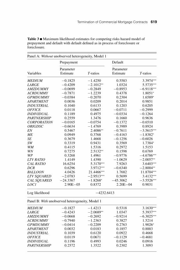
Table 3, Panel A, presents the results from fitting Model 1. If we combinethe effects of linear and square terms for the option variables, then borrowerswith large intrinsic values of the put (LTV RATIO) or call option (CAL RATIO)are more likely to default or prepay (see Figure 4A and B). Furthermore, theeffects of the intrinsic value of options on instantaneous prepayment and defaulthazards are convex. Prepayment is not sensitive to the intrinsic call value when itis out of the money, yet starts to increase very rapidly after CAL RATIO becomespositive and until it hits about 30% (see Figure 4). Mortgage default, however,begins to increase prior to the point of negative equity (Figure 4). This mayin part reflect noise in our measurement of property value as compared to our

26 For various definitions of default, and possible paths of a loan’s history, see Archeret al. (2000).


Figure 2 � NCREIF property value appreciation index by property type. The propertyindex is calculated from NCREIF appreciation returns from 1978 to 1998. Marshalland Swift construction cost figures are used as a substitute for years 1974–1977 whenthe NCREIF data were not available.

Appreciation Index for Four Property Types from 1974-1998

80

100

120

140

160

180

200

220

240

260

74 75 76 77 79 80 81 82 84 85 86 87 89 90 91 92 94 95 96 97

Year

Inde

x

Apartment

Industrial

Office

Retail

measurement of the call value. We also find that call (put) risks strongly affectthe exercise of put (call) options. Very large values of the put option (high LTVRATIO) reduce the likelihood of prepayment, while high values of the call option(high positive CAL RATIO) moderate the risk of default. These indirect effectsconfirm the significance of the joint nature of the two mortgage options and theimportance of modeling them as competing risks; by exercising the call (put)option, the borrower forfeits both the future default and prepayment options.The effect of contemporaneous LTV on prepayment risk may be explainedby institutional constraints on required equity levels necessary for borrowing.Highly negative CAL RATIO (deeply out of the money), however, is found toreduce the default hazard risk (see Figure 4B). We believe this result is causedby a small subsample of loans originated in the mid- to late 1970s that weresubsequently prepaid by borrowers upon property sale in the early 1980s, wheninterest rates were much higher.


Figure 3 � ACLI mortgage commitment rate versus mortgage coupon rate in thesample.

4

6

8

10

12

14

16

18

74/1

75/2

76/3

77/4

79/1

80/2

81/3

82/4

84/1

85/2

86/3

87/4

89/1

90/2

91/3

92/4

94/1

95/2

96/3

Year/Quarter

Per

cen

tag

e

ACLI Mean

Sample Mean

We find that contemporaneous insolvency, proxied by a low DCR, significantlyraises default risk while reducing prepayment risk, even after controlling forthe value of the put and call options. The significance of cash flow variables ondefault suggests that borrowers with negative equity do not default as long as in-come generated by the property is sufficient to cover scheduled debt payments.An alternative explanation is that borrowers in cash flow distress might defaultwith positive equity in their property.27 This seems to imply that the selling costsare quite high or additional short-term equity financing are very costly, render-ing them more expensive alternatives to default. Contrary to prior research, DCRat origination shows up mostly insignificant in the hazard functions for bothprepayment and default. This could result from borrowers engaging in “windowdressing” of their cash flow projections, similar to the behavior identified forcorporations prior to raising capital through debt or equity. Thus, original DCRcontains little information with respect to the termination outcome. This find-ing highlights the importance of including contemporaneous variables whenspecifying models of mortgage prepayment and default.

27 This phenomenon has been observed in earlier studies of commercial mortgage default(see Ciochetti and Riddiough 1998).


Table 2 � Descriptive statistics at origination and termination.

At Origination At Termination

All Loans Prepaid Defaulted All Loans Prepaid DefaultedVariable (N = 2,052) (N = 599) (N = 533) (N = 2,052) (N = 599) (N = 533)

Original 0.721 0.715 0.726 — — —LTV (0.058) (0.057) (0.048)

Original 1.259 1.261 1.217 — — —DCR (0.161) (0.118) (0.130)

LTV from 0.713 0.706 0.735 0.670 0.540 0.848index (0.075) (0.067) (0.084) (0.354) (0.197) (0.474)

DCR from 1.044 1.047 0.979 1.280 1.602 0.895index (0.259) (0.182) (0.199) (0.674) (0.755) (0.390)

CALL −0.026 −0.023 −0.010 0.026 0.027 0.0382OPTION (0.068) (0.068) (0.065) (0.047) (0.052) (0.0603)

Note: Standard deviations are in parentheses. Of the original descriptive sample of 2,090loans, 48 lacked complete information and were deleted for purposes of estimation. Thus,the estimation sample is comprised of 2,052 loans.

Borrowers of large loans are found to be more likely to default, but less likelyto prepay, while borrowers of smaller loans are more likely to prepay. This isinconsistent with the fixed-cost hypothesis that implies higher probabilities ofexercising the put or call option by borrowers of large loans. An alternativeexplanation could be that loan-size dummies capture differences in costs ofcapital and bargaining power in workout situations between borrowers ofdifferent loan size. Borrowers of smaller loans are usually charged highercoupon rates initially. Yet, as these borrowers gain more expertise in propertymanagement and accumulate more experience, they can obtain better financingarrangements. Lacking alternative means for low-cost borrowing, borrowers ofsmall loans might also resort to refinancing or selling in order to cash out equityfor personal consumption and/or business expansion. Borrowers of large loansmay have fewer incentives to protect their credit from default, possibly becauseof their well-established credit history, experience in property management, orownership structure. They are also more likely to exert influence in the ex postnegotiation with the lender since they can best manage the underlying propertysecuring the mortgage. Borrower type does not seem to affect either defaultor prepayment risks. Loan-size dummies appear to better capture the variationin borrowers’ bargaining power and credit availability than do borrower-typedummies.

Property type does not seem to affect default or prepayment risk. The insignif-icance of property type on default is in contrast to the findings of Vandell et al.


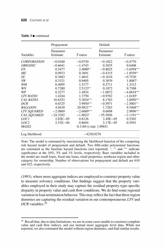
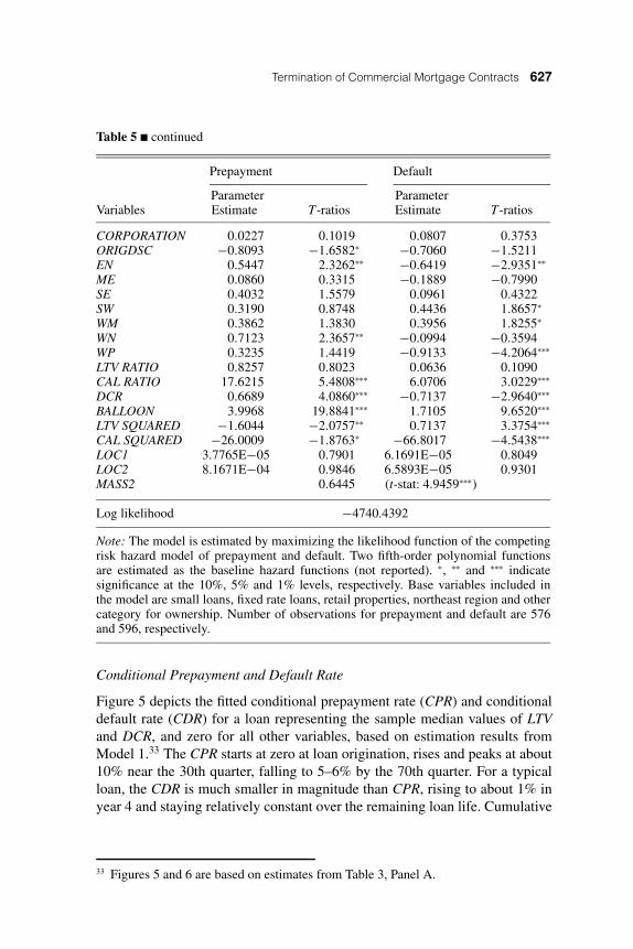
Table 3 � Maximum likelihood estimates for competing risks hazard model ofprepayment and default with default defined as in process of foreclosure orforeclosure.

Panel A: Without unobserved heterogeneity, Model 1

Prepayment Default

Parameter ParameterVariables Estimate T-ratios Estimate T-ratios

MEDIUM −0.1825 −1.4250 0.5583 3.3974∗∗∗

LARGE −0.4209 −2.1012∗∗ 1.0324 5.5735∗∗∗

AMZDUMMY −0.0699 −0.2849 −0.8953 −6.9118∗∗∗

ACRDUMMY −0.7871 −1.2239 0.4378 1.8051∗

GPMDUMMY −0.0384 −0.2070 0.2304 1.6589∗

APARTMENT 0.0036 0.0209 0.2014 0.9851INDUSTRIAL 0.1040 0.6133 0.1203 0.6205OFFICE 0.0118 0.0667 −0.0711 −0.2999INDIVIDUAL 0.1189 0.4975 −0.0334 −0.1264PARTNERSHIP 0.2559 1.3476 0.1660 0.9636CORPORATION −0.0165 −0.0754 −0.1372 −0.6510ORIGDSC −0.6634 −1.4769 0.3989 0.8924EN 0.5467 2.4086∗∗ −0.7611 −3.5615∗∗∗

ME 0.0949 0.3768 −0.4163 −1.8382∗

SE 0.3679 1.4668 −0.1256 −0.6026SW 0.3319 0.9431 0.3569 1.7384∗

WM 0.4115 1.5316 0.2972 1.5153WN 0.7275 2.5132∗∗ 0.1598 0.6769WP 0.3268 1.4961 −0.9776 −4.6786∗∗∗

LTV RATIO 1.4149 1.4390 −1.0629 −2.0057∗∗

CAL RATIO 16.6254 5.3170∗∗∗ 7.9263 3.6403∗∗∗

DCR 0.6296 3.9712∗∗∗ −0.6340 −2.8004∗∗

BALLOON 4.0426 21.4466∗∗∗ 1.7682 11.8704∗∗∗

LTV SQUARED −2.0783 −2.9513∗∗∗ 0.5699 3.4132∗∗∗

CAL SQUARED −24.3367 −1.8268∗ −45.3062 −3.5526∗∗∗

LOC1 2.90E−05 0.8372 2.20E−04 0.9031

Log likelihood −4232.6413

Panel B: With unobserved heterogeneity, Model 1

MEDIUM −0.1827 −1.4213 0.5318 3.1630∗∗∗

LARGE −0.4243 −2.0689∗∗ 1.0347 5.3937∗∗∗

AMZDUMMY −0.0668 −0.2692 −0.9214 −6.3025∗∗∗

ACRDUMMY −0.7940 −1.2363 0.3827 1.5214GPMDUMMY −0.0414 −0.2209 0.2763 1.9026∗

APARTMENT 0.0032 0.0183 0.1857 0.8883INDUSTRIAL 0.1039 0.6120 0.0922 0.4668OFFICE 0.0119 0.0671 −0.1129 −0.4681INDIVIDUAL 0.1196 0.4993 0.0246 0.0916PARTNERSHIP 0.2572 1.3522 0.2302 1.3093



Prepayment Default


CORPORATION −0.0160 −0.0730 −0.1022 −0.4770ORIGDSC −0.6641 −1.4743 0.3035 0.6408EN 0.5477 2.4000∗∗ −0.8025 −3.6594∗∗∗

ME 0.0933 0.3691 −0.4315 −1.8559∗∗

SE 0.3683 1.4641 −0.1616 −0.7530SW 0.3321 0.9405 0.3839 1.8087∗

WM 0.4095 1.5177 0.2711 1.3312WN 0.7280 2.5123∗∗ 0.1872 0.7388WP 0.3277 1.4924 −1.0072 −4.6818∗∗∗

LTV RATIO 1.4244 1.3750 −0.9782 −1.6185∗

CAL RATIO 16.6352 5.3024∗∗∗ 8.1763 3.0950∗∗∗

DCR 0.6325 3.9950∗∗∗ −0.5971 −2.5001∗∗

BALLOON 4.0430 20.9821∗∗∗ 1.7263 9.5468∗∗∗

LTV SQUARED −2.0869 −2.6689∗∗∗ 0.6698 2.9896∗∗∗

CAL SQUARED −24.3292 −1.8023∗ −55.5056 −3.1191∗∗∗

LOC1 2.82E−05 0.8126 3.49E−05 0.5302LOC2 2.51E−04 0.8694 2.17E−05 0.5591MASS2 0.1169 (t-stat: 1.0965)


Note: The model is estimated by maximizing the likelihood function of the competingrisk hazard model of prepayment and default. Two fifth-order polynomial functionsare estimated as the baseline hazard functions (not reported). ∗, ∗∗ and ∗∗∗ indicatesignificance at the 10%, 5% and 1% levels, respectively. Base variables included inthe model are small loans, fixed rate loans, retail properties, northeast region and othercategory for ownership. Number of observations for prepayment and default are 610and 422, respectively.

(1993), where more aggregate indices are employed to construct property valueto measure solvency conditions. Our findings suggest that the property vari-ables employed in their study may capture the residual property-type-specificdisparity in property value and cash flow conditions. We do find some regionalvariation in loan termination behavior. This may reflect the fact that these regiondummies are capturing the residual variation in our contemporaneous LTV andDCR variables.28

28 Recall that, due to data limitations, we are in some cases unable to construct completevalue and cash flow indices, and use instead more aggregate level data. While notreported, we also estimated the model without region dummies, and find similar results.


Figure 4 � Effects of call and put on prepayment and default hazard. Calculated basedon coefficients estimated in Table 3, Panel A. Effect on hazard rates equal to exp(xb1 +x2b2), where b1 and b2 are coefficients for the linear and squared terms, respectively.

Panel A: The Effect of LTV Ration on Prepayment and Default Hazard

0

10

20

30

40

50

60

0.6

0.64

0.68

0.72

0.76

0.8

0.84

0.88

0.92

0.96 1

1.04

1.08

1.12

1.16

1.2

1.24

1.28

1.32

1.36

1.4

1.44

1.48

1.52

LTV Ratio

Eff

ect o

n P

rep

aym

ent H

azar

d

-1

1

3

5

7

9

11

13

15

Eff

ect o

n D

efau

lt H

azar

d

PREPAYMENT

DEFAULT

Panel B: Effect of Call Ratio on Prepayment and Default Hazard

0

15

30

45

60

75

90

-20

-17

-14

-11 -8 -5 -2 1 4 7 10 13 16 19 22 25 28 31 34 37

CAL Ratio (%)

Eff

ect o

n P

rep

aym

ent H

azar

d

0

0.2

0.4

0.6

0.8

1

1.2

1.4

1.6

Eff

ect o

n D

efau

lt H

azar

d

Prepayment

Default

We find accrual and step-rate loans to be positively related to default risk,reflecting the increasing costs associated with keeping the mortgage optionalive as time goes by. These variables may also reflect self-selection at loaninitiation. Under asymmetric information, borrowers with higher default risks


will choose to take loans with lower initial payments. As loan balances increaseafter origination, borrowers of accrual and step-rate loans are much more likelyto default and less likely to prepay.

The balloon-year dummy exhibits a strong impact on both prepayment anddefault events. Prepayment immediately before maturity reflects the borrower’srisk aversion, but it has only a small effect on lender’s return. Default at balloonyear, however, reflects the value of the “wait-to-default” option for the borrower,and the resulting losses to the lender can be severe.29

Estimation with Unobserved Heterogeneity

Table 3, Panel B, reports results with bivariate unobserved heterogeneity(Model 2). The estimation shows no significant heterogeneity among borrow-ers in the risk of exercising call and put options as reflected by the lack ofsignificance of the MASS2 variable. The first risk group consists of 90% of thepopulation. However, the existence of two distinct groups is not statisticallysignificant.30

Qualitatively, the coefficients on the observed characteristics of the loans aresimilar to the case without heterogeneity. Deng, Quigley and Van Order (2000)and Follain, Ondrich and Sinha (1997) argue that ignoring heterogeneity canlead to biased estimates. Thus, the fact that there is little change in the parameterestimates offers indirect support for the lack of heterogeneity among borrowerswith respect to mortgage termination under the strict definition of default.

An ongoing concern related to commercial mortgage default analysis is theappropriate definition of mortgage default. ACLI reports loans as delinquentafter 60 days, while the National Association of Insurance Commission (NAIC)reports loans as delinquent at 90 days. Prior research on commercial mortgagedefault has included studies that construe default from as early as 90 daysdelinquent (Snyderman 1994 and Archer et al. 2000), to as long as actual loanforeclosure (Vandell et al. 1993). Yet, borrower behavior with respect to exerciseof the put option may vary considerably depending on the precise definition ofdefault.

To examine the extent to which default definition may impact the empiricalnature of the competing risk of prepayment and default, as well as the degree to

29 See for example Snyderman (1994), Esaki, L’Heureux and Snyderman (1999),Ciochetti and Riddiough (1998), or Ciochetti and Shilling (1999).30 MASS1 is normalized to 1 in the empirical estimation, so that the probability of beingin the first group is MASS1/(MASS1 + MASS2) = 1/(1 + 0.1169) = 90%.


which unobserved heterogeneity may be identified, we reestimate Models 1 and2 with two more expanded definitions of mortgage default. In the first case, wedefine default as all loans in process of foreclosure and foreclosed as in Table 3,but add loans that have experienced some form of renegotiation or modification(Table 4). We do so because renegotiation inevitably has an economic impacton both the borrower and lender in some form, through a reduction in the noterate, accrual provisions, forbearance and the like. We next expand the definitionof default further to include not only loans in process of foreclosure, foreclosedloans and renegotiated loans, but also those loans that are 90 days delinquent(Table 5). The extended definition of default reflects the borrower’s view ofdefault with respect to exercise, while the restricted definition, being moreclosely related to the default outcome, reflects the lender’s view. By extendingthe definition of default, our counts for prepaid and defaulted loans go from610 and 422, respectively, in Table 3, to 599 and 534, respectively, in Table 4and 576 and 596, respectively, in Table 5.31

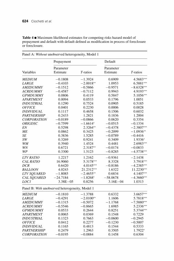
Qualitatively, we observe little difference in results from the maximum like-lihood estimation without unobserved heterogeneity (Model 1) using the ex-panded definitions of mortgage default. In most cases, we note that param-eter estimates are comparable as we move from a strict definition of default(Table 3, Panel A) to more broadly defined definitions (Tables 4 and 5,Panels A).

Of interest, however, are the estimation results with bivariate unobservedheterogeneity. While we found no significant heterogeneity among borrowersusing a strict definition of default (in process and foreclosed, Table 3, Panel B),we do find a statistically significant second mass point when we expand thedefinition of mortgage default as described above. Allowing heterogeneity alsosignificantly improves overall model performance, as reflected by the likelihoodratio statistics. When the default definition is expanded to include modifiedloans, group two is 40% of the sample (0.6702/(1 + 0.6702) = 0.4, see Table 4,Panel B). This group is about 18 times more likely to prepay and about 10% morelikely to default than the first group. When the definition of default is furtherextended to include delinquent loans, group two comprises 39% (0.6445/(1 +0.6445) = 0.39; see Table 5, Panel B). The second group is 22 times more likelyto prepay and 7% more likely to default than the first group. However, the esti-mated differences between the location parameters in both cases are statisticallyinsignificant.32 Thus, we are unable to contribute the source of heterogeneityas coming from prepayment or default. We postulate that the reason we find

31 Note that as we move from a strict definition of default, the number of prepaymentsdecreases.32 The numbers for prepayment and default are derived as LOC2/LOC1.


Table 4 � Maximum likelihood estimates for competing risks hazard model ofprepayment and default with default defined as modification in process of foreclosureor foreclosure.


Prepayment Default


MEDIUM −0.1808 −1.3924 0.6909 4.5683∗∗∗

LARGE −0.4103 −2.0018∗∗ 1.0953 6.5881∗∗∗

AMZDUMMY −0.1512 −0.5866 −0.9571 −8.6328∗∗∗

ACRDUMMY −0.4587 −0.7112 0.9943 4.9193∗∗∗

GPMDUMMY 0.0806 0.4119 0.5847 5.1056∗∗∗

APARTMENT 0.0094 0.0533 0.1796 1.0051INDUSTRIAL 0.1290 0.7524 0.0905 0.5185OFFICE 0.0401 0.2230 0.0006 0.0028INDIVIDUAL 0.1117 0.4658 0.1506 0.6032PARTNERSHIP 0.2433 1.2821 0.1836 1.2004CORPORATION −0.0189 −0.0866 0.0620 0.3354ORIGDSC −0.7599 −1.6614∗ −0.0515 −0.1334EN 0.5298 2.3264∗∗ −0.4378 −2.3807∗∗∗

ME 0.0862 0.3425 −0.2099 −1.0936∗∗

SE 0.3836 1.5285 −0.0789 −0.4416SW 0.3269 0.9241 0.3409 1.9336∗

WM 0.3940 1.4524 0.4481 2.6983∗∗∗

WN 0.6721 2.3187∗∗ −0.0174 −0.0833WP 0.3300 1.5123 −0.8285 −4.5738∗∗∗

LTV RATIO 1.2217 1.2162 −0.9361 −2.1438CAL RATIO 16.9060 5.3178∗∗∗ 8.3328 3.7918∗∗∗

DCR 0.6420 4.0145∗∗∗ −0.8186 −4.2385∗∗∗

BALLOON 4.0243 21.2312∗∗∗ 1.6322 11.2230∗∗∗

LTV SQUARED −1.8085 −2.4655∗∗ 0.6834 4.1407∗∗∗

CAL SQUARED −24.7184 −1.8268∗ −58.0678 −4.3660∗∗∗

LOC1 3.38E−05 0.8256 3.16E−04 1.0313


MEDIUM −0.1810 −1.3788 0.6332 3.6657∗∗∗

LARGE −0.4291 −2.0100∗∗ 1.1606 5.7818∗∗∗

AMZDUMMY −0.1315 −0.5072 −1.1768 −7.5880∗∗∗

ACRDUMMY −0.5546 −0.8665 1.6985 5.2336∗∗∗

GPMDUMMY 0.0533 0.2644 0.8251 5.3744∗∗∗

APARTMENT 0.0065 0.0369 0.1548 0.7229INDUSTRIAL 0.1323 0.7663 −0.0600 −0.2945OFFICE 0.0412 0.2277 −0.1230 −0.5007INDIVIDUAL 0.1165 0.4813 0.1544 0.5333PARTNERSHIP 0.2479 1.2963 0.3505 1.7922∗

CORPORATION −0.0195 −0.0884 0.1458 0.6304



Prepayment Default


ORIGDSC −0.7441 −1.6071 −0.6519 −1.3246EN 0.5363 2.3190∗∗ −0.7437 −3.2605∗∗∗

ME 0.0740 0.2895 −0.2901 −1.1679SE 0.3798 1.4907 −0.1337 −0.5604SW 0.3264 0.9062 0.3519 1.4445WM 0.3812 1.3777 0.4036 1.8111∗

WN 0.6847 2.3297∗∗ −0.0923 −0.3229WP 0.3336 1.5056 −1.0882 −4.7363∗∗∗

LTV RATIO 1.2348 1.2095 −0.1620 −0.2688CAL RATIO 17.0216 5.3527∗∗∗ 7.3919 2.8278∗∗∗

DCR 0.6551 4.1083∗∗∗ −0.9085 −3.8316∗∗∗

BALLOON 4.0237 20.7738∗∗∗ 1.5323 8.0287∗∗∗

LTV SQUARED −1.8434 −2.4106∗∗ 0.7651 3.4370∗∗∗

CAL SQUARED −24.6983 −1.8100∗ −71.1861 −4.1460∗∗∗

LOC1 2.95E−05 0.7942 4.00E−05 0.8009LOC2 5.44E−04 0.9044 4.41E−05 0.8629MASS2 0.6702 (t-stat: 4.6641∗∗∗)



some evidence of heterogeneity in the more relaxed definition of mortgagedefault is due to the increased set of possible outcomes. For example, bor-rowers with stronger market power may gain more from a negotiation pro-cess. The heterogeneity parameter may pick up this variation. This is in con-trast to the result with the more strict default definition, where decisions aremore costly to reverse, and, as a result, borrowers act in a more homogeneousmanner.

Consistent with Deng, Quigley and Van Order (2000), Tables 4 and 5 confirmthe importance of estimating a competing risk model with unobserved hetero-geneity. Although there is no qualitative change in parameter estimates, thereis significant change in their magnitude, especially for the coefficients on CALRATIO and DCR in the default hazard function.


Table 5 � Maximum likelihood estimates for competing risks hazard model ofprepayment and default with default defined as 90 days delinquency.


Prepayment Default


MEDIUM −0.2210 −1.6942∗ 0.6386 4.6352∗∗∗

LARGE −0.4062 −1.9759∗∗ 0.9864 6.4098∗∗∗

AMZDUMMY −0.1773 −0.6871 −0.9150 −8.4474∗∗∗

ACRDUMMY −0.4886 −0.7499 0.9475 4.5986∗∗∗

GPMDUMMY 0.1184 0.6019 0.6603 5.9749∗∗∗

APARTMENT 0.0020 0.0111 0.2117 1.2440INDUSTRIAL 0.1221 0.7124 0.2087 1.2884OFFICE 0.0469 0.2604 −0.0009 −0.0045INDIVIDUAL 0.1703 0.7108 0.0200 0.0874PARTNERSHIP 0.2887 1.5205 0.0520 0.3449CORPORATION 0.0262 0.1204 −0.0482 −0.2743ORIGDSC −0.8375 −1.7743∗ −0.1226 −0.3394EN 0.5272 2.3167∗∗ −0.4163 −2.3533∗∗

ME 0.0971 0.3859 −0.1311 −0.7088SE 0.3947 1.5731 0.1079 0.6428SW 0.3185 0.9031 0.3575 2.0599∗∗

WM 0.4007 1.4794 0.4459 2.7133∗∗

WN 0.6879 2.3497∗∗ −0.0264 −0.1297WP 0.3105 1.4243 −0.6983 −4.0045∗∗∗

LTV RATIO 0.7955 0.7888 −0.8402 −2.1073∗∗

CAL RATIO 17.3108 5.4098∗∗∗ 7.4147 4.1787∗∗∗

DCR 0.6394 3.9033∗∗∗ −0.6401 −3.4646∗∗∗

BALLOON 3.9959 20.8428∗∗∗ 1.7835 13.0687∗∗∗

LTV SQUARED −1.5353 −2.0747∗∗ 0.6497 4.3322∗∗∗

CAL SQUARED −26.0255 −1.9124∗ −55.1681 −4.7262∗∗∗

LOC1 4.81E−05 0.8272 6.08E−04 1.1700



MEDIUM −0.2211 −1.6573∗ 0.6388 4.0380∗∗∗

LARGE −0.4392 −2.0522∗∗ 1.0647 5.7203∗∗∗

AMZDUMMY −0.1544 −0.5889 −1.0700 −7.1747∗∗∗

ACRDUMMY −0.6416 −0.9996 1.6365 4.8333∗∗∗

GPMDUMMY 0.0760 0.3718 0.8354 5.6527∗∗∗

APARTMENT −0.0094 −0.0523 0.1987 0.9803INDUSTRIAL 0.1171 0.6708 0.1496 0.7913OFFICE 0.0411 0.2248 −0.0684 −0.2955INDIVIDUAL 0.1699 0.6935 0.0875 0.3276PARTNERSHIP 0.2974 1.5336 0.2050 1.1037



Prepayment Default


CORPORATION 0.0227 0.1019 0.0807 0.3753ORIGDSC −0.8093 −1.6582∗ −0.7060 −1.5211EN 0.5447 2.3262∗∗ −0.6419 −2.9351∗∗

ME 0.0860 0.3315 −0.1889 −0.7990SE 0.4032 1.5579 0.0961 0.4322SW 0.3190 0.8748 0.4436 1.8657∗

WM 0.3862 1.3830 0.3956 1.8255∗

WN 0.7123 2.3657∗∗ −0.0994 −0.3594WP 0.3235 1.4419 −0.9133 −4.2064∗∗∗

LTV RATIO 0.8257 0.8023 0.0636 0.1090CAL RATIO 17.6215 5.4808∗∗∗ 6.0706 3.0229∗∗∗

DCR 0.6689 4.0860∗∗∗ −0.7137 −2.9640∗∗∗

BALLOON 3.9968 19.8841∗∗∗ 1.7105 9.6520∗∗∗

LTV SQUARED −1.6044 −2.0757∗∗ 0.7137 3.3754∗∗∗

CAL SQUARED −26.0009 −1.8763∗ −66.8017 −4.5438∗∗∗

LOC1 3.7765E−05 0.7901 6.1691E−05 0.8049LOC2 8.1671E−04 0.9846 6.5893E−05 0.9301MASS2 0.6445 (t-stat: 4.9459∗∗∗)



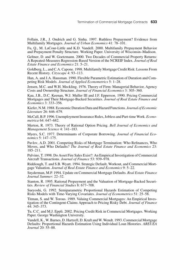
Conditional Prepayment and Default Rate

Figure 5 depicts the fitted conditional prepayment rate (CPR) and conditionaldefault rate (CDR) for a loan representing the sample median values of LTVand DCR, and zero for all other variables, based on estimation results fromModel 1.33 The CPR starts at zero at loan origination, rises and peaks at about10% near the 30th quarter, falling to 5–6% by the 70th quarter. For a typicalloan, the CDR is much smaller in magnitude than CPR, rising to about 1% inyear 4 and staying relatively constant over the remaining loan life. Cumulative

33 Figures 5 and 6 are based on estimates from Table 3, Panel A.


Figure 5 � Estimated conditional quarterly default and prepayment. Baseline functionis estimated by fitting fifth-order polynomial functions. Median sample values of LTVand DCR ratios are used to compute the predicted conditional default and prepaymentrates. CAL RATIO is set to zero.

Conditional Prepay/Default Rate by Quarter

0.00

0.02

0.04

0.06

0.08

0.10

0.12

1 4 7 10 13 16 19 22 25 28 31 34 37 40 43 46 49 52 55 58 61 64 67 70

Quarters

Co

nd

itio

nal

Pre

pay

men

t Rat

e

0.00

0.01

0.02

0.03

0.04

0.05

Con

ditio

nal D

efau

lt R

ate

Prepayment hazard (Left Axis)

Default hazard (Right axis)

prepayment and default rates are shown in Figure 6. These results are generallyconsistent with those found in prior research.

Robustness Discussion

In this section, we discuss the robustness of our results relative to issues ofmeasurement errors as well as specification of the baseline hazard function.

We recognize that the aggregate indices are not perfect substitutes for individual-level property value and cash flow information, since they may underestimateloan-level volatility.34 By definition, half of the properties perform better and

34 By construction, the NCREIF index is smoothed and contains spurious seasonality.The seasonality is caused by a concentration of outside appraisals at the end of calendaryear (see Geltner and Goetzmann 2000).


Figure 6 � Estimated cumulative prepayment and default rate. Baseline function isestimated by fitting fifth-order polynomial functions. Median sample values of LTVand DCR ratios are used to compute the predicted conditional default and prepaymentrates. CAL RATIO is set to zero.

Cumulative Prepayment and Default Rates

0.00

0.10

0.20

0.30

0.40

0.50

0.60

0.70

0.80

0.90

1.00

1 4 7 10 13 16 19 22 25 28 31 34 37 40 43 46 49 52 55 58 61 64 67 70

Quarters

Cu

mu

lati

ve R

ate

Prepayment

Default

half worse than the indices. Moreover, average ACLI mortgage commitmentrates fail to reflect the actual availability and exact rates of refinancing creditto a specific borrower with particular credit history. The unobserved prepay-ment penalty may introduce additional noise in the measurement of call values.Measurement errors in the calculated contemporaneous property, loan, and NOIvalues will be inherent in the LTV, CAL and DCR ratios. Empirical estimationwill thus lead to (downward) biased estimates of the coefficients, which maymake generalization of results more difficult.

Three features in our research design mitigate the measurement error problemsin the hazard regression. First, variables highly correlated with the measurementerrors are included as observed heterogeneity variables. For example, contem-poraneous LTV and DCR can affect the availability and cost of credit, and theyare included in the hazard function of prepayment. Second, unobserved bivariateheterogeneity can partially control for the measurement error through locationparameters. For example, loans with underestimated/overestimated propertyvalues will likely be grouped into the category with a high/low value of loca-tion parameter of default to compensate for the underestimation in the defaulthazard rate. Finally, a flexibly specified baseline will capture the underestima-tion of volatility from using aggregate indices in estimating individual loan


information. As time passes, the value and cash flow performance of individ-ual properties will deviate further away from the index level by accumulatingmore idiosyncratic risks. In other words, the issue of measurement error willbecome more severe over time. However, the baseline hazard can trend up tooffset the underprediction in the prepayment and default hazard due to the lackof cross-sectional variability in loan-level variables (LTV, CAL and DCR) overtime.

An additional concern is the effect of a misspecification of the baseline func-tion on our model estimates. The empirical estimation of the hazard model inthis paper assumes a fifth-order polynomial function as the baseline function.To check the robustness of our results to the functional form of baseline haz-ard, we estimate our model using Cox Partial Likelihood (CPL) specification,which does not require specification of a baseline function form. As shown inTable 6, the estimation generates qualitatively similar results to Table 3, Panel A,with the exception that additional region dummies help explain prepaymentbehavior.

Conclusions and Implications

This study is the first to examine commercial mortgage default and prepaymentin a competing risk hazard framework using loan-level data. We explicitlymodel prepayment and default as a joint mortgage termination option. Ourempirical findings are largely consistent with the predictions from the theory ofcontingent claims and prior empirical research using residential mortgage data.High values of put and call options greatly increase the default and prepaymentrisk in a nonlinear (convex) manner. The value of the put/call option is alsofound to significantly affect the exercise of the call/put option, thus capturingthe competing-risk nature of the two termination events.

We also show that option pricing theory alone is not adequate to explain com-mercial mortgage defaults and prepayments. The financial sophistication, bar-gaining power, solvency and credit history of borrowers also affect the mortgagetermination decision by shifting the exercise boundary of both the prepaymentand default options.

In contrast to prior research on residential mortgages, we find no evidenceof unobserved heterogeneity among mortgage borrowers under a strict defini-tion of mortgage default. However, we do find some evidence of unobservedheterogeneity under more general definitions of mortgage default. Relative toresearch conducted on commercial mortgages, this study confirms the impor-tance of using contemporaneous information as proxies for the theoretic putand call variables. Interestingly, after controlling for contemporaneous debt


Table 6 � Cox Partial Likelihood estimates for the independent risks of mortgageprepayment and default; Model 3.

Prepayment Default


MEDIUM −0.1520 −1.4067 0.5602 3.5508∗∗∗

LARGE −0.4463 −2.7249∗ 1.0378 6.0130∗∗∗

AMZDUMMY −0.1096 −0.6131 −0.8707 −6.9006∗∗∗

ACRDUMMY −0.9528 −1.5768 0.4423 1.9467∗

GPMDUMMY −0.0377 −0.2403 0.2321 1.7657∗

APARTMENT −0.0754 −0.4984 0.2396 1.2316INDUSTRIAL 0.0339 0.2358 0.1380 0.7651OFFICE −0.0726 −0.4821 −0.0273 −0.1288INDIVIDUAL 0.0453 0.2452 −0.0456 −0.1795PARTNERSHIP 0.2742 1.8146∗ 0.1640 0.9941CORPORATION −0.0710 −0.4142 −0.1427 −0.7166ORIGDSC −0.6836 −2.0688∗∗ 0.4638 1.3718EN 0.6895 3.8430∗∗∗ −0.7583 −3.6502∗∗∗

ME 0.1016 0.4959 −0.4500 −2.0859∗∗

SE 0.3588 1.7673∗ −0.1416 −0.7195SW 0.4404 1.5117 0.3478 1.7175∗

WM 0.4750 2.2726∗∗ 0.2732 1.4497WN 0.6293 2.7052∗∗ 0.1600 0.7091WP 0.3835 2.2489∗∗ −0.9960 −5.0246∗∗∗

LTV RATIO 4.5204 3.5242∗∗∗ −1.6769 −3.7777∗∗∗

CAL RATIO 19.1887 10.4329∗∗∗ 8.5096 5.7021∗∗∗

DCR 1.1559 6.8365∗∗∗ −0.9632 −3.9931∗∗∗

BALLOON 4.0527 30.5772∗∗∗ 1.4975 10.5479∗∗∗

LTV SQUARED −3.7043 −4.3114∗∗∗ 0.6981 5.1238∗∗∗

CAL SQUARED −33.9775 −3.7705∗∗∗ −53.4456 −5.3917∗∗∗

Log likelihood −3282.69 −2568.27

Note: The model is estimated with Cox’s Partial Likelihood (CPL) approach, whichdoes not require specification of baseline hazard functions. Prepayment and defaultfunctions are estimated separately. Base variables included in the model are small loans,fixed rate loans, retail properties, northeast region, and other category for ownership. Inthe estimation for one risk, termination events by the other risk are taken as censored.The value of the Partial Log Likelihood is not comparable to the Full Log LikelihoodValue one in the competing risk specification of Tables 4 and 5. ∗, ∗∗ and ∗∗∗ indicatesignificance at the 10%, 5% and 1% levels, respectively.

coverage ratio, we find no evidence to suggest that original debt coverage ratiois related to commercial mortgage default. This is in contrast to prior work,which fails to include contemporaneous cash flow information in the empiricalmodel specification.


Our results have important practical implications. We establish empirically thataggregate indices contain valuable information about the performance of indi-vidual loans and demonstrate how to incorporate such information efficientlythrough a hazard model framework. Future default and prepayment paths can bepredicted by simulating property value and interest rate processes to allow forthe pricing of whole loans and their securitized counterparts. The competing-risks methodology is also applicable to regulators in order to set efficient min-imum capital requirement for institutions involved in commercial mortgagelending. As exogenous observable variables shift the option’s exercise bound-ary and affect mortgage terminations through the transaction cost structure,they should be explicitly considered in both the underwriting and the pricingof commercial mortgages. These important issues warrant continued research.

We thank Jim Shilling and Brent Ambrose for helpful comments and suggestions. Weare also grateful to David Ling and three anonymous referees for their comments andsuggestions.

References

Ambrose, B. and T. Sanders. 2001. Commercial Mortgage-Backed Securities. WorkingPaper. Ohio State University.Archer, W.R., E.J. Elmer, D.M. Harrison and D.C. Ling. 2002. Determinants of Multi-family Mortgage Default. FDIC Real Estate Economics 30: 445–473.Brown, D.T., B.A. Ciochetti and T.J. Riddiough. 2000. Liquidity Provision and LiquidityTransformation in the Resolution of Financial Distress. Working Paper. University ofNorth Carolina.Ciochetti, B.A. and T.J. Riddiough. 1998. Timing, Loss Recovery, and Economic Per-formance of Foreclosed Commercial Mortgages. Working Paper. University of NorthCarolina.Ciochetti, B.A. and J.D. Shilling. 1999. Default Losses and Commercial Mortgages.Working Paper. University of North Carolina.Cox, D.R. 1972. Regression Models and Life-Tables. Journal of the Royal StatisticalSociety, Series B (Methodological) 34: 187–220.Cox, D.R. 1975. Partial Likelihood. Biometrika 62: 269–276.Cox, D.R. and D. Oakes. 1984. Analysis of Survival Data. Chapman and Hall: London.Deng, Y. 1997. Mortgage Termination: An Empirical Hazard Model with a Stochas-tic Term Structure. Journal of Real Estate Finance and Economics 14: 309–331.Deng, Y., J.M. Quigley and R. Van Order. 1996. Mortgage Default and Low Downpay-ment Loans: The Costs of Public Subsidy. Regional Science and Urban Economics 26:263–285.Deng, Y., J.M. Quigley and R. Van Order. 2000. Mortgage Terminations, Heterogeneityand the Exercise of Mortgage Options. Econometrica 68: 275–307.Elmer, P.J. and A.E. Haidorfer. 1997. Prepayments of Multifamily Mortgage-BackedSecurities. Journal of Fixed Income 6: 50–63.Esaki, H., S. L’Heureux and M. Snyderman 1999. Commercial Mortgage Defaults: AnUpdate. Real Estate Finance 16: 81–86.


Follain, J.R., J. Ondrich and G. Sinha. 1997. Ruthless Prepayment? Evidence fromMultifamily Mortgages. Journal of Urban Economics 41: 78–101.Fu, Q., M. LaCour-Little and K.D. Vandell. 2000. Multifamily Prepayment Behaviorand Prepayment Penalty Structure. Working Paper. University of Wisconsin–Madison.Geltner, D. and W. Goetzmann. 2000. Two Decades of Commercial Property Returns:A Repeated-Measures Regression-Based Version of the NCREIF Index. Journal of RealEstate Finance and Economics 21: 5–21.Goldberg, L., and C.A. Capone. 1998. Multifamily Mortgage Credit Risk: Lessons FromRecent History. Cityscape 4: 93–113.Han, A. and J.A. Hausman. 1990. Flexible Parametric Estimation of Duration and Com-peting Risk Models. Journal of Applied Econometrics 5: 1–28.Jensen, M.C. and W.H. Meckling. 1976. Theory of Firm: Managerial Behavior, AgencyCosts and Ownership Structure. Journal of Financial Economics 3: 305–360.Kau, J.B., D.C. Keenan, W.J. Muller III and J.F. Epperson. 1990. Pricing CommercialMortgages and Their Mortgage-Backed Securities. Journal of Real Estate Finance andEconomics 3: 333–356.Kiefer, N.M. 1988. Economic Duration Data and Hazard Functions. Journal of EconomicLiterature 26: 646–679.McCall, B.P. 1996. Unemployment Insurance Rules, Jobless and Part-time Work. Econo-metrica 64: 647–682.Merton, R. 1973. Theory of Rational Option Pricing. Bell Journal of Economics andManagement Science 4: 141–183.Myers, S.C. 1977. Determinants of Corporate Borrowing. Journal of Financial Eco-nomics 5: 147–175.Pavlov, A.D. 2001. Competing Risks of Mortgage Termination: Who Refinances, WhoMoves, and Who Defaults? The Journal of Real Estate Finance and Economics 23:185–211.Pulvino, T. 1998. Do Asset Fire Sales Exist?: An Empirical Investigation of CommercialAircraft Transactions. Journal of Finance 53: 939–978.Riddiough, T. and S.B. Wyatt. 1994. Strategic Default, Workout, and Commercial Mort-gage Valuation. Journal of Real Estate Finance and Economics 9: 5–22.Snyderman, M.P. 1994. Update on Commercial Mortgage Defaults. Real Estate FinanceJournal Summer: 22–32.Stanton, R. 1995. Rational Prepayment and the Valuation of Mortgage-Backed Securi-ties. Review of Financial Studies 8: 677–708.Sueyoshi, G. 1992. Semiparametric Proportional Hazards Estimation of CompetingRisks Models with Time-Varying Covariates. Journal of Econometrics 51: 25–58.Titman, S. and W. Torous. 1989. Valuing Commercial Mortgages: An Empirical Inves-tigation of the Contingent-Claims Approach to Pricing Risky Debt. Journal of Finance44: 345–373.Tu, C.C. and M.J. Eppli. 2002. Pricing Credit Risk in Commercial Mortgages. WorkingPaper. George Washington University.Vandell, K., W. Barnes, D. Hartzell, D. Kraft and W. Wendt. 1993. Commercial MortgageDefaults: Proportional Hazards Estimation Using Individual Loan Histories. AREUEAJournal 20: 55–88.

Date post:	08-Jul-2020
Category:	Documents
Upload:	others
View:	25 times
Download:	0 times

The Termination of Commercial Mortgage Contracts through...

Documents