THE TIME VALUE OF MONEY - University of South Floridasbesley.myweb.usf.edu/FIN3403/notes/tvm.pdf ·...

The Time Value of Money - 1

THE TIME VALUE OF MONEY (Chapter 4) The concepts presented in this section are used in nearly every financial decision, whether it is a business decision or a decision that relates to your personal finances. As a result, time value of money is considered the most important concept in finance. • Cash Flow Time Lines—a very important tool that helps you to visualize the timing of the cash

flows associated with a particular situation. A cash outflow is designated with a negative sign, whereas a cash inflow is designated with a positive sign (in most cases the positive sign is implied). The interest rate that is applied to the situation is given on the time line. A cash flow time line can be illustrated as follows:

According to this cash flow time line, we want to determine how much $500 invested today will grow to in four years if the investment earns 10 percent interest per year (for simplicity, the dollar sign is not shown).

• Future Value (FV)—when we find the future value of an amount invested today, we determine to

what amount the investment will grow over a particular time period. If an amount is invested for more than one period, then both the original investment and any interest previously earned by the investment will earn interest when additional interest is paid—this concept, where interest earns interest, is known as compounding; that is, compounded interest is earned. In the example given in the cash flow time line shown above, we have

If we summarize the computations using the portion of each computation, we have the following:

FV1 = PV(1 + r)1 FV2 = PV(1 + r)2 FV3 = PV(1 + r)3 FV4 = PV(1 + r)4

Using the pattern shown here, we can conclude that determining the future value of an amount invested today for n years, FVn, can be found by applying the following equation:

FVn = PV(1 + r)n

According to this equation, the simple solution to our current situation—that is, the future value of the $500 investment at the end of four years if 10 percent return is earned—would be:

-500 ?

10% Time Cash Flows

0 1 2 3 4

-500 x 1.10 x 1.10 x 1.10 x 1.10

10% End-of-year amount

0 1 2 3 4

= 550.00 = 605.00 = 665.50 = 732.05


FV4 = $500(1.10)4 = $732.05

which is the same as the result found earlier. There are four general approaches we can take to arrive at this solution—(1) time line solution, (2) equation (numerical) solution, (3) financial calculator, and (4) spreadsheet solution. o Time Line Solution—the solution is shown graphically on a cash flow time line o Equation (Numerical) Solution—the numerical solution is determined by applying the

appropriate equation, which in this case is FVn = PV(1 + r)n. o Financial Calculator Solution—financial calculators have been programmed to give you the

numerical solution for many time value of money situations. The keys that are used for such problems are:

N

I/Y

PV

PMT

FV

where N is the number of periods, I/Y is the interest rate per period, PV is the present value of the amount, PMT represents an annuity payment (discussed later), and FV is the future value. Using a financial calculator, the current situation would be set up as follows:

Inputs:

4

10

-500

0

?

N

I/Y

PV

PMT

FV

Result:

= 732.05

This illustration indicates the calculator inputs—you input N = 4 for the number of periods, I/Y = 10 for the interest rate (notice that interest is not input as a decimal because the calculator does the conversion for you), PV = -500 for the present value, (the 500 investment should have a negative sign because it represents a cash outflow), and PMT = 0 for the annuity payment (there is no annuity payment). Once these values are entered, you are ready to compute the future value, FV, which equals 732.05.

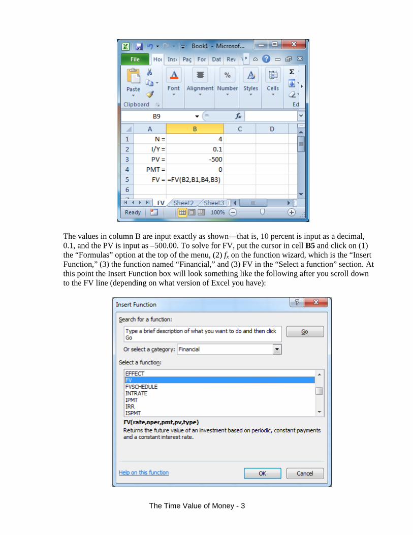
o Spreadsheet Solution—spreadsheets, such as Excel or Lotus 1-2-3, have functions that can be used to solve time value of money problems. Using Excel 2010, the current problem can be set up as follows:


The values in column B are input exactly as shown—that is, 10 percent is input as a decimal, 0.1, and the PV is input as –500.00. To solve for FV, put the cursor in cell B5 and click on (1) the “Formulas” option at the top of the menu, (2) fx on the function wizard, which is the “Insert Function,” (3) the function named “Financial,” and (3) FV in the “Select a function” section. At this point the Insert Function box will look something like the following after you scroll down to the FV line (depending on what version of Excel you have):


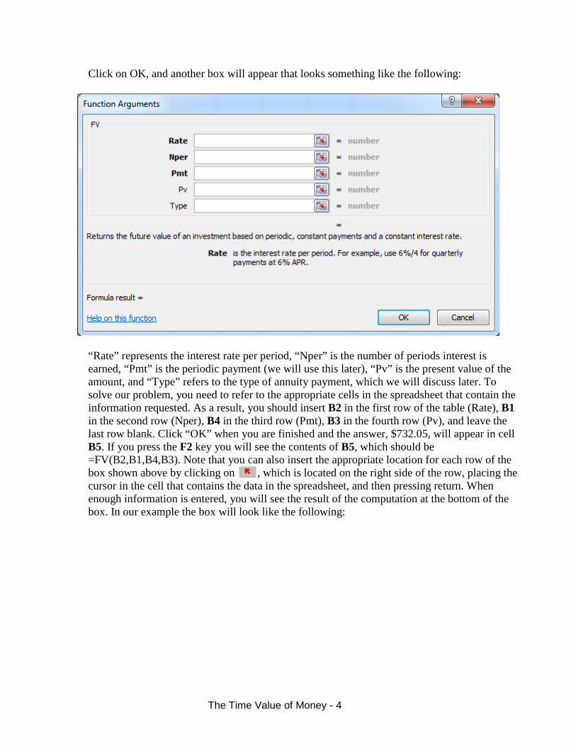
Click on OK, and another box will appear that looks something like the following:

“Rate” represents the interest rate per period, “Nper” is the number of periods interest is earned, “Pmt” is the periodic payment (we will use this later), “Pv” is the present value of the amount, and “Type” refers to the type of annuity payment, which we will discuss later. To solve our problem, you need to refer to the appropriate cells in the spreadsheet that contain the information requested. As a result, you should insert B2 in the first row of the table (Rate), B1 in the second row (Nper), B4 in the third row (Pmt), B3 in the fourth row (Pv), and leave the last row blank. Click “OK” when you are finished and the answer, $732.05, will appear in cell B5. If you press the F2 key you will see the contents of B5, which should be =FV(B2,B1,B4,B3). Note that you can also insert the appropriate location for each row of the box shown above by clicking on , which is located on the right side of the row, placing the cursor in the cell that contains the data in the spreadsheet, and then pressing return. When enough information is entered, you will see the result of the computation at the bottom of the box. In our example the box will look like the following:


Once the locations of all the appropriate data are in the table, click “OK,” and the answer will appear in cell B5 in the spreadsheet.

The future value amount that we computed here, $732.05, is equivalent to the present value amount, $500, compounded at 10 percent for four years. Thus, all else equal, if someone asked you whether you would prefer $500 today or $732.05 in four years and you have the opportunity to earn 10 percent per year, you should say that both options are the same and, as a result, you should “flip a coin” to choose between the two. Consider what would happen if you have $500 today and you invested it at 10 percent for four years—the value at the end of four years would be $732.05. Consider what would happen if you had a piece of paper (contract) that stated you were guaranteed a payment of $732.05 in four years and you could earn 10 percent during the next four years—as we will see in the next section, the value today of the $732.05 to be received in four years is $500, so you could sell your right to receive (the contract) the $732.05 to someone else and receive $500 today. In other words, if you chose one option—either PV = $500.00 or FV = $732.05—you always can create the other option.

• Future Value of an Annuity (FVA)—an annuity is defined as a series of equal payments that are

made at equal intervals; for example, $100 received each year for the next five years. An ordinary annuity is an annuity with cash flows that occur at the end of the period, whereas an annuity due is an annuity with cash flows that occur at the beginning of the period. We can determine the future value of an annuity, whether it is an ordinary annuity or an annuity due, by using the concepts described earlier for solving for the future value of a lump-sum amount. o Ordinary annuities—suppose you decide to plan for your retirement, which will occur soon, by

making payments equal to $10,000 at the end of each of the next four years. If the investment will earn a return equal to 7 percent per year, what will be the value of your investment at the end of three years? The cash flow time line is:


Time Line Solution: Using the methodology presented earlier to determine the FV of a

single amount invested today, we have the following (be careful—think about the number of periods each payment earns interest):

Equation (Numerical) Solution: The solution given in the cash flow time line shows that

the future value of an annuity, FVAn, can be determined by computing the future values, FVs, of each individual payment and summing the result. In other words,

FVA3 = 10,000(1.07)2 + 10,000(1.07)1 + 10,000(1.07)0 = 11,449 + 10,700 + 10,000 = 32,149

Notice that the first payment, PMT1, only earns two years of interest because it is invested at the end of the first year—interest is earned in Year 2 and Year 3; the second payment, PMT2, only earns one year of interest—interest is earned in Year 3; and, the third payment, PMT3, earns no interest because it is invested at the end of the final year. In general terms, we can write the computation given above as follows:

=

=

∑∑ r1 - )r + (1 PMT = )r + (1 PMT = )r + (1 PMT

)r + PMT(1 + ... + )r + PMT(1 + )r + PMT(1 + )r + PMT(1 FVAn

tn-n

1=t

t1n-

0=t

03n-2n-1n-n

You determine the future value of the annuity, FVA, by calculating the future value of each payment and summing the results, as was shown previously, or by applying the final form of the equation given above. It is important to recognize that this equation can only be used for determining the future value of an annuity—it cannot be used to determine the future value of a series of cash flows that are not equal (such a series is termed an uneven cash flow pattern; its solution will be discussed later).

-10,000 -10,000 -10,000

7% Time Cash Flows

0 1 2 3

FVA3 = ?

10,000 10,000 10,000 = 10,000(1.07)0

7% 0 1 2 3

10,700 = 10,000(1.07)1 11,449 = 10,000(1.07)2 32,149 = FVA3


149,32$ = )2149.30(000,1$ = 70.0

1 - )7(1.0 0000,1$ =FVA

r1 - )r + (1 PMT = FVA

3

3

n

n

This is the same result that was found by computing the future values of each payment and summing the results.

Equation (Numerical) Solution:

Inputs:

3

7

0

–10,000

?

N

I/Y

PV

PMT

FV

Result:

= 32,149

In this situation, we need to use the time value of money key labeled PMT because we are dealing with an annuity. Notice that the input into PV is 0 because we are not using this key.

Spreadsheet Solution: The problem can be set up as follows:

To solve for the future value of the annuity, put the cursor in cell B5 and click on (1) the “Formulas” option at the top of the menu, (2) fx on the function wizard, which is the “Insert Function,” (3) the function named “Financial,” and (3) FV in the “Select a function” section. In the box that appears, input the cell locations of the appropriate values as shown earlier.


o Annuities due—because an annuity due is an annuity with cash flows at the beginning of the period, each payment will earn interest for one more period than if it was an ordinary annuity, and the future value of the annuity will be greater, all else equal.

Time Line Solution—Graphically, we have the following situation:

Notice that the computations are the same as for an ordinary annuity, except one additional period (year) of interest is given to each payment.

Equation (Numerical) Solution: As the cash flow time line solution shows, to compute the

future value of an annuity due, which is designated FVA(DUE)n, the future value of each payment is multiplied by an additional year’s interest, 1.07 in this case. Thus, we need to make a simple adjustment to the equation used to compute the future value of an ordinary annuity to determine the future value of an annuity due. The adjustment is to multiply the interest factor for an ordinary annuity by (1 + r), which yields the following:

10,000 10,000 10,000 10,700.00 = 10,000(1.07)1

7% 0 1 2 3

11,449.00 = 10,000(1.07)2 12,250.43 = 10,000(1.07)3 34,399.43 = FVA(DUE)3


n

n

3

(1 + r - 1)FVA(DUE = PMT (1 + r))r

(1.07 - 1) = $10,000 (1.07)0.07

= $10,000[(3.2149)(1.07)] = $10,000(3.439943) = $

×

×

34,399.43

Financial Calculator Solution: By default, most financial calculators are programmed to

compute the value of an ordinary annuity. But, your calculator should have a key that allows you to switch from end-of-period payments to beginning-of-period payments. The key generally is labeled DUE, BEG, BGN, or has some similar labeling (the key might be a secondary function). To solve this problem, you need to switch your calculator to BGN so that the cash flows are considered beginning-of-period payments.

BGN

Inputs:

3

7

0

-10,000

?

N

I/Y

PV

PMT

FV

Result:

= 34,399.43

As you can see, to solve for an annuity due, the inputs remain the same—you only need to switch the calculator to beginning-of-period payments.

Spreadsheet Solution: Set up the problem as for an ordinary annuity. After clicking on the

financial function FV, input the cell locations of the appropriate values as before, and input a 1 in the row labeled “Type,” which indicates that the payments are made at the beginning of the period. In the current example, the inputs are the same as previously, except a 1 is input for “Type” such that the following exists:


Click “OK” when you are finished and the answer, $34,399.43, will appear in cell B5 of the

spreadsheet. • Future Value of Uneven Cash Flow Streams, FVCFn—unlike an annuity, an uneven cash flow

stream consists of cash flows that are not all the same (equal), so the simplifying techniques (that is, using a single equation) we just presented to compute the values of annuities cannot be used here. o Future value of an uneven cash flow stream—consider the following situation: Time Line Solution:

As the cash flow time line illustrates, to determine the FV of this cash flow stream, we must compute the future value of each individual cash flow and sum the resulting values.

Equation (Numerical) Solution: The general equation used to compute the future value of

an uneven cash flow stream is:

According to this equation, you must compute the future value of each cash flow, CFt, and then sum the results. Note that we will use CF to designate cash flows, whether they are uneven or equal, and PMT to designate annuity payments (discussed in previous sections). The solution to the current problem is:

( ) ( ) ( )2 1 03 600 1 04 400 1 04 200 1 04

600 1 0816 400 1 0400 200 1 0000648 96 416 00 200 001 264 96

FV CF = . + . . = ( . ) ( . ) ( . )

. . ., .

+

+ += + +=

Financial Calculator Solution: You can use the cash flow register on your financial

calculator to solve this problem. You must input the cash flows in the order they occur—that is, first input CF1, then input CF2, and so on. Most calculators require you to input a value for CF0 before entering any other cash flows—CF0 represents the cash flow in the current period. In the current situation, there is no cash flow in the current period, so CF0 =

0 1 2 3 -600 -400 -200.00 = 200(1.04)0 416.00 = 200(1.04)1 648.96 = 600(1.04)2 FVCF3 = 600(1.04)2 + 400(1.04)1 + 200(1.04)0 = 1,264.96

r = 4%

23 1 2

1 nn

nt

tt=1

FV CF = CF (1 + r CF (1 + r CF (1 + r) ) )

= CF (1 + r)

+ + +

∑


0 must be entered. After entering the cash flows, enter the value for I/Y = r, and then press NPV to compute the present value (NPV stands for the net present value, which is the present value of the future cash flows plus the cash flow in the current period). Then, remember that FV = PV(1 + r)n. You should refer to the instructions that came with your calculator to determine exactly how uneven cash flows must be entered. If you have a Texas Instruments BAII PLUS, solve for the present value for the current problem using these steps:

Press CF0= 0 should be displayed

Press This clears any numbers that might be in the CF register from previous work. CF0= 0 appears in the display. In this problem CF0= 0, so we do not input a value for CF0.

Press , enter 600 and press C01= 600 should be displayed

Press F01= 1 should be displayed, which indicates that the frequency for C01 (number of times C01 appears) is 1

Press , enter 400 and press C02= 400 should be displayed

Press F02= 1 should be displayed, which indicates that the frequency for C02 is 1

Press , enter 200 and press C03= 200 should be displayed. At this point, all the

cash flows have been input into the CF registers.

Press I= 0 should be displayed

Enter 4 and press , press NPV= 0 should be displayed

Press NPV= 1,124.544834 should be displayed—this is the PV of the cash flows given on the time line

FV = 1,124.5445(1.04)3 = 1,264.9596 = 1,264.96

CF

2nd CLR Work

ENTER

ENTER

ENTER

NPV

ENTER

CPT



To solve for the future value of the future cash flows, put the cursor in cell B4 and click on the “financial” function named NPV. In the box that appears input the following cell locations:

The range C2:E2 contains the values of the cash flows for Year 1 through Year 3. When


you click “OK” you will see the answer, $1,124.54, appear in cell B4. Remember that this represents to PV of the uneven cash flow stream. As a result, you need to compute the FV of $1,124.54, which is FV = $1,124.544834(1.04)3 = $1,264.96.

• Present Value (PV)—PV is the value of an amount to be received (or paid) in the future stated in

today’s (present) dollars—that is, the current value of a future amount. When we find the present value, PV, of an amount we are said to be discounting the future value to the present at the opportunity cost rate, which is the rate that can be earned on an investment with equal risk. If we have the opportunity to earn a positive rate of return, the present value must always be less than the future value—the positive return ensures that an amount that is invested today grows to a greater amount in the future. In essence, when we compute the PV of a future amount, we take out the interest that the amount would earn during the time it is invested—that is, we “deinterest” the FV.

o Time Line Solution: On a cash flow time line we can illustrate present value as follows:

In this case, we want to determine the present value of $800 that is to be received in four years if the opportunity cost is 8 percent. To solve this problem, let’s “plug” the known information into the equation given earlier for determining the future value of an amount invested today:

FVn = PV(1 + r)n 800 = PV(1 + 0.08)4

Rearranging the terms, we have

02.588)735030.0(800

= )408(1.

1 008 = )48(1.0

008 = PV

==

×

According to this computation, we can determine the present value of an amount to be received (paid) in the future using the same equation we applied to determine the future value of an amount invested today. Thus, the solution for the PV of a lump-sum amount is:

Solving for the current situation using the methods described earlier, we have:

)r + (11

FV = )r + (1

FV = PV nnnn

Time 0 1 2 3 4 Cash Flows PV = ? 800

8%

0 1 2 3 4 End-of-year amount 588.02 635.07 685.87 740.74 800.00

8%

÷1.08 ÷1.08 ÷1.08 ÷1.08


o Equation (Numerical) Solution:

02.588 = )735030(0. 008 = )8(1.0

1 800= PV 4

×

o Financial Calculator Solution:

Inputs:

4

8

?

0

800

N

I/Y

PV

PMT

FV

Result:

= -588.02

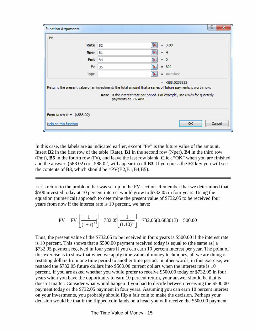
o Spreadsheet Solution: The problem can be set up as follows:

To solve for the future value of the annuity, put the cursor in cell B3 and click on (1) the “Formulas” option at the top of the menu, (2) fx on the function wizard, which is the “Insert Function,” (3) the function named “Financial,” and (3) PV in the “Select a function” section. At this point a box will appear that looks something like the following:


In this case, the labels are as indicated earlier, except “Fv” is the future value of the amount. Insert B2 in the first row of the table (Rate), B1 in the second row (Nper), B4 in the third row (Pmt), B5 in the fourth row (Fv), and leave the last row blank. Click “OK” when you are finished and the answer, (588.02) or –588.02, will appear in cell B3. If you press the F2 key you will see the contents of B3, which should be =PV(B2,B1,B4,B5).

Let’s return to the problem that was set up in the FV section. Remember that we determined that $500 invested today at 10 percent interest would grow to $732.05 in four years. Using the equation (numerical) approach to determine the present value of $732.05 to be received four years from now if the interest rate is 10 percent, we have:

00.500)683013.0(05.732)10.1(

105.732)r1(

1FVPV 4nn ==

=

+

=

Thus, the present value of the $732.05 to be received in fours years is $500.00 if the interest rate is 10 percent. This shows that a $500.00 payment received today is equal to (the same as) a $732.05 payment received in four years if you can earn 10 percent interest per year. The point of this exercise is to show that when we apply time value of money techniques, all we are doing is restating dollars from one time period to another time period. In other words, in this exercise, we restated the $732.05 future dollars into $500.00 current dollars when the interest rate is 10 percent. If you are asked whether you would prefer to receive $500.00 today or $732.05 in four years when you have the opportunity to earn 10 percent return, your answer should be that is doesn’t matter. Consider what would happen if you had to decide between receiving the $500.00 payment today or the $732.05 payment in four years. Assuming you can earn 10 percent interest on your investments, you probably should flip a fair coin to make the decision. Perhaps your decision would be that if the flipped coin lands on a head you will receive the $500.00 payment


today, and if it lands on a tail you will receive the $732.05 payment in four years. Suppose that the coin is flipped and lands on a head and you are paid $500.00 today. After you take the payment, you decide you don’t need the money now, but would rather wait four years to receive the money. In this case, as we showed in the previous section, you can invest the $500.00 at 10 percent for four years and it will grow to $732.05. Now suppose that the coin is flipped and it lands on a tail and you receive a piece of paper (a contract) that states whoever turns in the “paper” in four years will be paid $732.05. After you receive the “paper,” however, you decide that it would be better to have money today so that you can pay off some of your credit card debt. As the above computation shows, you should be able to sell the “paper” to another investor for $500.00 today (assuming all investors have an opportunity interest rate equal to 10 percent). As a result, the two options—$500.00 payment today or $732.05 payment in four years—are equally desirable if the opportunity interest rate is 10 percent. (We also assume that there is no risk associated with the future payment.)

• Present Value of an Annuity (PVA)—we can determine the present value of an annuity, whether it

is an ordinary annuity or an annuity due, by using the concepts described earlier where we solved for the present value of a lump-sum amount. o Ordinary annuities—suppose you win a contest and the prize is that you will receive three

annual payments equal to $10,000 each beginning in one year. If you have an opportunity to earn a 7 percent return on your investments, how much is this annuity worth to you today? In other words, for how much could you sell this annuity to someone today?

Time Line Solution:

Equation (Numerical) Solution: The solution given in the cash flow time line shows that the present value of an annuity, PVAn, can be determined by computing the present values, PVs, of each individual payment and summing the results. In other words,

16.243,2698.162,839.734,8345.79,9

(1.07)

1$10,000 (1.07)

1$10,000 (1.07)

1$10,000 PVA 3313

=++=

+

+

=

Using the relationships given here, we can give a general equation for computing the present value of an ordinary annuity:

10,000 10,000 10,000

7% 0 1 2 3

10,000/(1.07)1 = 9,345.79 10,000/(1.07)2 = 8,734.39 10,000/(1.07)3 = 8,162.98 PVA3 = 26,243.16


r

- 1 PMT =

)r + (11PMT + ... +

)r + (11PMT +

)r + (11PMT +

)r + (11PMT = PVA

)r+ (11

n321n

nk

Applying this equation to our situation, the solution is

Financial Calculator Solution:

Inputs:

3

7

?

10,000

0

N

I/Y

PV

PMT

FV

Result:

= –26,243.16

Notice that the input into FV is 0 because we are not using this key.

Spreadsheet Solution: To solve the problem, set up the spreadsheet the same as you would to solve for the PV of a lump-sum amount (single payment), and input values in the appropriate cells. The current problem can be set up as follows:

16.243,26= )624316.20(000,1 = 070.

- 1 0000,1 =

r

- 1 PMT = PVA

)07(1.1

)r + (11

n

3n


o Annuities due—How would the present value of the annuity examined above differ if it was an annuity due? Remember that the cash flows associated with an annuity due occur at the beginning of the period rather than the end of the period, which is the case for an ordinary annuity.

Time Line Solution: In our situation, if the cash flows occur at the beginning of the period,

the cash flow time line would be as follows:

Equation (Numerical) Solution: The cash flow time line above shows that the adjustment

to the present value is simply to add another year’s interest to each payment. Thus, the equation used to find the present value of an ordinary annuity can be applied as follows to find the present value of an annuity due:

18.080,28 = )808018.20(000,1 = )]07(1. 624316.20[000,1 =

)07(1. 070.

- 1 0000,1 =

)r + (1 r

- 1 PMT = )PVA(DUE

)07(1.1

)r + (11

n

3

n

×

×

×

Calculator Solution: To solve this problem, you need to switch your calculator to the BGN

mode so that the cash flows are considered beginning-of-period payments.

BGN Inputs:

3

7

?

10,000

0

N

I/Y

PV

PMT

FV

Result:

= -28,080.18

As you can see, to solve for an annuity due the inputs remain the same—you only need to switch the calculator to beginning-of-period payments.

Spreadsheet Solution: Set up the problem the same as for an ordinary annuity. After

clicking on the financial function PV, input the cell locations of the appropriate values as before, and input a 1 in the row labeled “Type,” which indicates that the payments are made a the beginning of the period.

10,000 10,000

7% 0 1 2 3

10,000/(1.07)0 = 10,000.00 10,000/(1.07)1 = 9,345.79 10,000/(1.07)2 = 8,734.39 PVA3 = 28,080.18


• Present Value of Uneven Cash Flow Streams, PVFCn—unlike an annuity, an uneven cash flow stream consists of cash flows that are not all the same (equal), so the simplifying techniques (that is, using a single equation) we just presented to compute the values of annuities cannot be used here.

o Time Line Solution: Consider the following situation:

As the cash flow time lines illustrates, to determine the PV of this cash flow stream, we must compute the present value of each individual cash flow and sum the resulting values.

o Equation (Numerical) Solution: The general equation used to compute the present value of an

uneven cash flow stream is:

According to this equation, you must compute the present value of each cash flow, CFt, and then sum the results. The solution to the current problem is:

3 1 2 3

1 1 1600 400 2001 04 1 04 1 04

600 0 96154 400 0 92456 200 0 88900576 924 369 824 177 800 1124 5481124 55

PVFC( . ) ( . ) ( . )

( . ) ( . ) ( . ). . . , .

, . (rounding difference)

= + +

= + += + + ==

o Financial Calculator Solution: You should use the cash flow register on your calculator to

solve this problem. See the explanation of how to compute the FV of an uneven cash flow stream using your calculator that was given in an earlier section. To find the PV of the uneven cash flow stream, simply compute the NPV of the cash flows.

o Spreadsheet Solution: See the explanation of how to compute the FV of an uneven cash flow

stream using a spreadsheet that was given in an earlier section. To find the PV of the uneven cash flow stream, enter values into the appropriate locations, and compute the NPV.

• Perpetuities—a perpetuity is an annuity that continues forever—that is, a perpetual annuity. The present value of a perpetuity can be computed using the following equation:

rPMT = PVP =

perpetuity aof luePresent va

r = 4% 0 1 2 3 600/(1.04)1 = 576.9231 600 400 200 400/(1.04)2 = 369.8225 200/(1.04)3 = 177.7993 PVFC3 = 1,124.5449

3 1 2 2

1 1 1 1n

n t1 n tt=1

P VFC = CF CF CF = CF(1 + r (1 + r (1 + r (1 + r) ) ) )

+ + +

∑


Suppose you were offered the opportunity to receive $250 beginning in one year and continuing forever. If you could earn 10 percent on your investments, how much should you pay for this perpetuity? The solution is:

$2,500 = 0.10$250 =

rPMT = PVP

• Comparison of PVA, FVA, and Lump-Sum Amount—in the previous sections, we found the

following:

Remember that when we compute the present value (PV), we take out, or “discount” a future

amount by the interest that the amount will earn in future periods. Similarly, when we compute the future value (FV), we add in, or “compound” a present amount by the interest it will earn over the investment period. As a result, the present value of a future amount and the future value of a present amount are the same values, but they are adjusted for the interest that can be earned during the investment period. To illustrate, assume you win a contest that offers you the choice of the following prizes. You can only pick one prize, and there is no risk associated with any of the choices. Your opportunity cost is 7 percent, regardless of which prize you choose. Which prize should you choose?

Prize A Payment of $26,243.16 today. Prize B Payment of $10,000 each year for the next three years; the first $10,000 is

scheduled to paid one year from today. Prize C Payment of $32,149 in three years. Your answer should be that it doesn’t matter which prize is selected, because they are all

equivalent. They are equivalent because you can create each of the prizes from one of the other prizes. Consider what would happen if you were required to randomly select one of the prizes—that is, you were required to draw from three pieces of paper that were put in a hat. Perhaps you want Prize A because you need to pay some bills today, but you draw the piece of paper with Prize C written on it. You should be able to sell Prize C to someone for $26,243.16, because the PV of $32,149 at 7 percent is $26,243.16 when the interest that would be earned during the next three years is taken out of the future amount.

16.243,26$16.243,26)816298.0(149,32$)07.1(

1149,32$PV 3 ===

=

Of course, the opposite is true as well—that is, if someone draws Prize A, he or she could invest

the $26,243.16 at 7 percent and it would grow to $32,149 in three years. Also, because we know that the PV of the 3-year $10,000 ordinary annuity is $26,243.16 if the opportunity cost is 7

10,000 10,000 10,000

7% 0 1 2 3

PVA3 = 26,243.16 32,149.00 = FVA3


percent, Prizes A and B must be the same. And, we know that the FV of the same annuity is $32,149, which means that Prizes B and C must be the same.

If you draw Prize A, but you want Prize B, you can create the same cash flow stream paid by Prize

B by investing the $26,243.16 at 7 percent and paying yourself $10,000 at the end of each of the next three years. The following table shows that this is true:

Beginning Year Amount Interest @7% Ending Balance Withdrawal 1 $26,243.16 $1,837.02 = 26,243.16 x 0.07 $28,080.18 = 26,243.16 + 1,837.02 $10,000 2 18,080.18 1,265.61 = 18,080.18 x 0.07 19,345.79 = 18,080.18 + 1,265.61 10,000 3 9,345.79 654.21 = 9,345.79 x 0.07 10,000.00 = 9,345.79 + 654.21 10,000 After the last $10,000 is withdrawn from the investment, the balance in the account is $0. • Solving for Time and Interest Rates—to this point, we have included four variables in the

equations for PV and FV—that is, PV, FV, r, and n. If three of the variables are known we can solve for the fourth variable; consider the following examples: o Solving for r—suppose you invested $200 three years ago, and the investment is now worth

$245. What rate of return (r) did the investment earn? Time Line Solution:

“Plugging into” the FV equation (you could also plug into the PV equation) gives the following:

Equation (Numerical) Solution: Using algebra to solve for r, we find that r = 7.0%:

( )

( )

( )%0.707.010700.1r

0700.12250.1r1

2250.1200245r1

r1200245

)3/1(

3

3

==−===+

==+

+=

)r + 00(12$ = 45$2 3

Time (Year) 0 1 2 3 Cash Flows -200 245

r = ?



Inputs:

3

? -200

0

245

N

I/Y

PV

PMT

FV

Result:

= 7.0


To solve for the interest rate, put the cursor in cell B2 and click on (1) the “Formulas” option at the top of the menu, (2) fx on the function wizard, which is the “Insert Function,” (3) the function named “Financial,” and (3) RATE in the “Select a function” section. At this point a box will appear that looks something like the following:


The labels are as indicated earlier. Insert B1 in the first row of the table (Nper), B4 in the second row (Pmt), B3 in the third row (Pv), B5 in the fourth row (Fv), and leave the last row blank. Click “OK” when you are finished and the answer, 7.0% (or, 0.07), will appear in cell B2. If you press the F2 key you will see the contents of B2, which should be =RATE(B1,B4,B3,B5)

o Solving for n—Suppose you invest $712 today at a 6 percent return. How long will it take for

the investment to grow to 848? The cash flow time line for this problem is:

“Plugging into” the FV equation (you could also plug into the PV equation) gives the following:

$712 = $848(1.06)n

Equation (Numerical) Solution: Unless you are good with algebra, the easiest way to approach this problem applying the numerical solution is to use a “trial-and-error” process whereby you plug in different values for n until you find the appropriate number of years—that is, the point where the right side of the equation and the left side of the equation are equal, or the FV of $712 invested at 6 percent equals $848. You should find that n = 3 years.


… 0 1 2 n = ? -712 848

6% Time

Cash Flows


Inputs:

?

6 -712

0

848

N

I/Y

PV

PMT

FV

Result: = 3.0


To solve for the number of years, put the cursor in cell B1 and click on fx on the function wizard, and then select NPER in the financial category. At this point a box will appear that looks something like the following:


The labels are as indicated earlier. Insert B2 in the first row of the table (Rate), B4 in the second row (Pmt), B3 in the third row (Pv), B5 in the fourth row (Fv), and leave the last row blank. Click “OK” when you are finished and the answer, 3.0, will appear in cell B1. If you press the F2 key you will see the contents of B1, which should be =NPER(B2,B4,B3,B5).

• Solving for Interest Rates with Annuities—The current value of an investment that will pay $300

each year for three years is $817. What rate of return (r) will the investment earn?

o Time Line Solution:

o Equation (Numerical) Solution: Using the equation developed earlier to find the present value of an ordinary annuity, we have the following:

r

- 1 300 =817

r

- 1 PMT = PVA

)r+ (11

)r + (11

n

3

n

0 1 2 3 300 300 300

r = ?

PVA = -817


To solve, use a trial-and-error process in which you substitute different values for r until the right side of the equation equals 817. Eventually you should find r = 5%. It is much easier to solve this problem using a financial calculator or a spreadsheet.


Inputs:

3

? -817

300

0

N

I/Y

PV

PMT

FV

Result:

= 5.0

o Spreadsheet Solution: The problem can be solved using the RATE function available in the spreadsheet. See the explanation in the previous section. Enter the known values into the appropriate cells, and then solve for the interest rate (r) using the RATE function.

• Solving for r with uneven cash flow streams—if you do not have a financial calculator, you must

use trial-and-error to solve for r if the cash flows are uneven. If you have a financial calculator, enter the future cash flows in the CF register as described earlier, enter the current value, or price, of the investment as CF0, which should be given, and then press the IRR key. IRR, which stands for the internal rate of return, will be discussed in detail in a later section. The solution using a spreadsheet is similar to the financial calculator solution—the IRR function is used. Consider the cash flows given earlier—that is, CF1 = 600, CF2 = 400, and CF3 = 200. What rate of return would you earn if you invested (paid) $970 today to receive these future cash flows?

o Time Line Solution:

o Equation (Numerical) Solution: The problem is set up as follows:

)r + (11 200 +

)r + (11 400 +

)r + (11 600 = 970 321

Using a trial-and-error method to solve for r, you will eventually find that 13.93 is the correct answer.

o Financial Calculator Solution: Input the value of each cash flow in the cash flow register of your calculator as shown previously, except input CF0 = –970, which represents the amount that would have to be paid to receive the future cash flows. As a result, the values in the cash flow register should be CF0 = –970, CF1 = 600, CF2 = 400, and CF3 = 200. After the cash flows have been input, press and then press ; the answer, 13.93 will be displayed. If you invest $970 to receive the cash flow stream given in the cash flow time line shown above, you will earn a 13.93 percent return.

0 1 2 3 -970 600 400 200

r = ?

CPT IRR


o Spreadsheet Solution: The problem can be set up as follows:

To solve for the rate of return on this investment, put the cursor in cell B3 and click on the financial function named IRR. In the box that appears input the following cell locations:

The range B2:E2 contains the values of the cash flows for Year 0 through Year 3. You do not have to input a value for “guess,” which represents a number you think the return might be. When you click “OK” the answer, 13.93, will appear in cell B3.

• Semiannual and Other Compounding Periods—to this point, we have assumed that interest is earned (computed) annually. In many instances, interest is computed more than once a year—that is, interest compounds, or is paid, during the year. For example, bonds generally pay interest twice each year (every six months), thus interest is compounded semiannually for such investments. In other instances, interest might be compounded more frequently—perhaps quarterly, monthly, or


even daily. Suppose that you invest $200 today in an investment that pays 8 percent interest, compounded quarterly, for a period of two years. In this case, at the end of the first quarter, which is three months from the time the investment starts, your investment account would receive its first interest payment such that the value at that time would be

204$ = )200(1.02$ = 4080. + 1002$ =

quarterfirst theofend at the Value

= FV 11

1

Each quarter, the rate paid is 2 percent. Thus, at the end of the second quarter, when the second interest payment is made, the value is

08.208$ = )200(1.02$ = quarter second theofend at the Value

= FV 22

In general, when computing either the present value or the future value, whether for a lump-sum amount or an annuity, you must adjust both the interest rate and the number of periods—divide the interest by the number of compounding periods in the year such that the rate represents the rate per interest period (8%/4 = 2% per quarter in our example), and multiply the number of years by the number of compounding periods in each year such that the value represents the total number of compounding periods (interest computations) during the entire investment period (2 years × 4 = 8 periods in our case). Applying this to the current situation, we have: o Time Line Solution:

In this case, r = 2% because the 8 percent rate is compounded quarterly, which means the rate per period is 8%/4 = 2%, and n = 8 because there are 8 quarters in a 2-year period—that is, 2 years × 4 quarters per year = 8 quarters. Using the concepts developed earlier, the solution to this problem is:

o Equation (Numerical) Solution:

FV = $200(1.02)8 = $200(1.171659) = $234.33


Inputs:

8

2

-200 0

?

N

I/Y

PV

PMT

FV

Result:

= 234.33

Year 0 1 2 Quarter 0 1 2 3 4 5 6 7 8 200.00 204.00 208.08 212.24 216.49 220.82 225.23 229.74 243.33

2%

x 1.02 x 1.02 x 1.02 x 1.02 x 1.02 x 1.02 x 1.02 x 1.02


o Spreadsheet Solution: The same adjustments that are made for the equation (numerical) solution and the financial calculator solution are required if you are using a spreadsheet. See the explanations given earlier that show how to set up the spreadsheet solution. Similar adjustments need to be made when determining the present value of a lump-sum amount, the present value of an annuity, and the future value of an annuity when compounding occurs more than once during the year—that is, the r must be stated so that it represents the rate per compounding period and n must be stated so that it represents the number of compounding periods that occur during the entire investment period.

• Effective (Equivalent) Annual Rate (rEAR)—When there is more than one compounding period in a

year, the effective annual interest rate (rEAR), which is the rate at which an investment actually increases (grows) each year, will be greater than the simple, or quoted, interest rate (rSIMPLE), which is the rate used to compute the amount of interest that is paid each compounding period. For example, in our current situation, the interest payments made in the first year of the investment would be:

Period Computation Interest per Period Quarter 1 FV1 = $200.00(1.02) = $204.00 $4.00 Quarter 2 FV2 = $204.00(1.02) = $208.08 4.08 Quarter 3 FV3 = $208.08(1.02) = $212.24 4.16 Quarter 4 FV4 = $212.24(1.02) = $216.48 4.24

Total = $16.48

Thus, the $200 initial investment would earn interest equal to $16.48, which means the effective, or actual, return on the investment is:

%24.8 = 08240. = 00.002$

48.16$ r=)EAR( rate annual Effective EAR =

This same return occurs year after year. In general terms, we can compute the effective annual rate of return for any investment (or other situation) using the following equation:

1.0m

r + 1 = r = rate annual

Effective SIMPLEm

EAR −

where rSIMPLE represents the quoted (simple) rate used to compute the interest payment each period and m is the number of interest payments, or compounding periods, per year. (rSIMPLE is often called the annual percentage rate, APR.) Applying this equation to our example, the EAR is

rEAR = (1.02)4 – 1.0 = 0.08243 = 8.243%

which is the same result we computed earlier.

The EAR can be used to compute the FV of the $200 investment, but now n = 2 years is used because we have converted the simple, non-compounded interest rate into its equivalent effective rate per year, rEAR. Using rEAR, the computation for FV would be:


FVn = PV(1 + rEAR)n = $200(1.08243)2 = $234.33

which is the same result we found earlier when adjusting both the interest rate and the number of periods for the number of compounding periods in the year.

• Amortized Loans—most consumer loans, such as mortgages and automobile loans, and some

business loans are amortized, which means that the loan agreement requires equal periodic payments, a portion of which constitutes interest on the debt and the remainder is applied to the repayment of the debt. It is important to understand what portion of the payment is interest and what portion is repayment of debt, because, when applicable, only the interest portion is considered an expense for tax purposes. An amortization schedule is used to determine what portion of the total payment is interest and what portion is repayment of principal.

To construct an amortization schedule, let’s consider the following situation: Suppose you borrow

$6,655 to make repairs to your house, and the loan is considered a second mortgage. The terms of the loan require you to make payments every three months—that is, quarterly—(beginning in three months) for the next two years and the simple interest rate (APR), is 6 percent. The first question you should ask is: What is the amount that must be paid every six months? Using a financial calculator, the solution is:

o Financial Calculator Solution: Remember to adjust I/Y = r so that it represents the rate per

payment period and N so that it represents the total number of payments associated with the loan.

Inputs:

8

1.5

6,655

?

0

N

I/Y

PV

PMT

FV

Result:

–889.00

Thus, the required loan payment each quarter is $889. Given this information, we can now construct an amortization schedule, which shows how much of each periodic payment is payment of interest and how much represents the repayment of the debt. The process is rather simple—start with the amount owed and compute the dollar interest on that amount; the principal repayment is the total periodic payment less the computed dollar interest. Because the periodic payment remains the same and the amount owed decreases each period, the amount of interest paid must decrease each period and the amount of principal repaid must increase each period. The amortization schedule for our situation is:


Beginning Periodic Interest Amount Repayment of Principal Ending Amt Owed Payment [ = (1) x 0.015 ] [ = (2) – (3) ] Amount Owed

PMT (1) (2) (3) (4) [ = (1) – (4) ] 1 $6,655.00 $889 $99.83 $789.17 $5,865.83 2 5,865.83 889 87.99 801.01 5,064.82 3 5,064.82 889 75.97 813.03 4,251.79 4 4,251.79 889 63.78 825.22 3,426.57 5 3,426.57 889 51.40 837.60 2,588.97 6 2,588.97 889 38.83 850.17 1,738.80 7 1,738.80 889 26.08 862.92 875.88 8 875.88 889 13.14 875.86 0.02* $7,112 = $457.02 + $6,654.98*

* Rounding difference

The values in the above amortization schedule can be generated using your calculator. The following steps show you how to generate an amortization schedule using a Texas Instruments BAII PLUS. For more information or if you have a different type of calculator, refer to the instructions manual that came with the calculator. For the current example, follow these steps:

1. Enter the information for the amortized loan into the TVM registers as was described earlier

to compute PMT = 889. 2. Enter the amortization function by pressing (“Amort” is written above the

key, which indicates it is a secondary function). P1 = 1 is displayed, which indicates the starting point for the amortization schedule is the first period. Press , and P2 = 1 is displayed, which indicates the ending point for the first set of computations is the first period.

3. a. Press , and BAL = 5,865.823316 is displayed. This indicates that the remaining principal balance at the end of the first quarter (three months) after the first payment is $5,865.82.

b. Press , and PRN = –789.1766837 is displayed, which indicates that the amount of principal repaid in the first period is $789.18.

c. Press , and INT = –99.825 is displayed, which indicates that the amount of interest paid in the first period is $99.83.

4. Press , and P1 = 2 is displayed; then press , and P2 = 2 is displayed, which indicates that the next series of computations relate to the second payment. Follow the same procedures given in Step 3, and you should see the following results: a. Press ; display shows BAL = 5,064.808982. b. Press ; display shows PRN = –801.0143339. c. Press ; display shows INT = –87.98734974.

5. Continue Step 4 and you will discover that the results for the remaining periods are the same values given previously in the table and shown in the spreadsheet that follows. If you use a calculator to construct a complete amortization schedule, you must repeat Step 4 for each year the loan exists—that is, Step 4 must be repeated six more times for the loan we use in this example. However, if you would like to know either the balance, principal repayment, or interest paid in a particular period, you need only set P1 and P2 equal to that period to display the desired values.

2nd PV

CPT

PV


o Spreadsheet Solution: You can set up an amortization schedule using a spreadsheet with the following relationships:

NOTE: The $ sign is included to fix the locations of the cells that contain common values that are required for each computation so that you can use the copy command to copy the relationships from row 6 to rows 7 through 13. The functions named IPMT and PPMT can be found in the financial section of the Formulas menu.


The numerical results should be as follows:

• Chapter 4 Summary Questions—You should answer these questions as a summary for the chapter

and to help you study for the exam. o Why is a dollar received today worth more than a dollar received in the future? o What is the concept of future value? Present value? What is the difference between the two? o What is the difference between an annuity, a lump-sum payment, and an uneven cash flow

stream? o What is the difference between an ordinary annuity and an annuity due? Give examples of each

type of annuity. o What is an amortized loan? What are its characteristics? o What is the effective annual rate (EAR)? How does the EAR differ from the APR (annual

percentage rate)?

Date post:	19-Mar-2018
Category:	Documents
Upload:	vothuy
View:	220 times
Download:	3 times

THE TIME VALUE OF MONEY - University of South Floridasbesley.myweb.usf.edu/FIN3403/notes/tvm.pdf ·...

Documents