The Time Variation of Risk and Return in Foreign Exchange...

The Time Variation of Risk and Return in Foreign Exchange Markets: A GeneralEquilibrium Perspective

Geert Bekaert

The Review of Financial Studies, Vol. 9, No. 2. (Summer, 1996), pp. 427-470.

Stable URL:

http://links.jstor.org/sici?sici=0893-9454%28199622%299%3A2%3C427%3ATTVORA%3E2.0.CO%3B2-5

The Review of Financial Studies is currently published by Oxford University Press.

Your use of the JSTOR archive indicates your acceptance of JSTOR's Terms and Conditions of Use, available athttp://www.jstor.org/about/terms.html. JSTOR's Terms and Conditions of Use provides, in part, that unless you have obtainedprior permission, you may not download an entire issue of a journal or multiple copies of articles, and you may use content inthe JSTOR archive only for your personal, non-commercial use.

Please contact the publisher regarding any further use of this work. Publisher contact information may be obtained athttp://www.jstor.org/journals/oup.html.

Each copy of any part of a JSTOR transmission must contain the same copyright notice that appears on the screen or printedpage of such transmission.

The JSTOR Archive is a trusted digital repository providing for long-term preservation and access to leading academicjournals and scholarly literature from around the world. The Archive is supported by libraries, scholarly societies, publishers,and foundations. It is an initiative of JSTOR, a not-for-profit organization with a mission to help the scholarly community takeadvantage of advances in technology. For more information regarding JSTOR, please contact [email protected].

http://www.jstor.orgMon Jan 14 12:13:48 2008


http://www.jstor.org/about/terms.html

http://www.jstor.org/journals/oup.html

The Time Variation of Risk and Return in Foreign Exchange Markets: A General Equilibrium Perspective Geert Bekaert Stanford University

This article successively introduces variable velocity, durability, and habitpersistence in a standard two-country general equilibrium model and explores their effects on the variability of exchange rate changes, forward premiums, and the foreign exchange risk premium A new fea- ture of the model is that agents make decisions at a weekly frequency and face conditionally heteroskedastic shocks. Nevertheless, even the most complex model fails to deliver sufficiently variable risk premiums without causing fomuardpre- rniums and exchange rates to be excessively variable. Unlike previous models, the model can roughly match the persistence of forward premiums.

Foreign exchange markets continue to confound international financial economists. For example, exchange rate changes seem excessively volatile relative

This article has benefited from the comments and suggestions of Tim Boller- slev, Jonas Fisher, Steve Grenadier, David Marshall, Ravi Jagannathan (the editor), Ken Singleton, Mark Watson, and the participants in seminars at Carnegie-hlellon University, UBC, University of Chicago, Stanford Univer- sity, UCW. University of Pennsylvania, the Wharton School, Yale Univer- sity, Columbia University, New York University, INSEAD, the University of Illinois, the Summer Meeting of the Econometric Society in Seattle. The Sloan School at hlIT, the Haas School of Business at UC Berkeley, and the 1993 Joint Statistical Meet~ngs in San Francisco. Special thanks go to Robert Modrick for his many suggestions and continuous encouragement and an anonymous referee whose thorough comments greatly improved this article. Financial support from a Sloan Dissertation Fellowship, an NSF grant, the Financial Services Research Intiatrve, and the Bass Fellowship of the Graduate School of Business at Stanford is gratefully acknowledged. Ad- dress all correspondence to Geen Bekaert, Graduate School of Business, Stanford University, Stanford. CA 94305-5015.

The Review of Financial Studies Summer 1996 Vol. 9, No, 2, pp. 427-470 @ 1996 The Review of Financial Studies 0893-945419615 1.50

to economic fundamentals [Meese (199011. Also, the forward rate is not an unbiased predictor of the future spot rate, implying predictable variation in excess returns in foreign exchange markets. Although a time-varying risk premium may explain this phenomenon, the required variability of this risk premium seems excessively large relative to the variability of potential sources of risk.' These two empirical phenomena are related. Highly volatile exchange rates increase the risks of international investments, which cannot be costlessly hedged in the forward market because unbiasedness is violated.

In this article, I develop a two-country monetary general equilibrium model that potentially explains these two anomalies. Building on the framework in Lucas (1978), the only friction in the model is the presence of transaction costs, which give rise to money being valued in equilibrium and induce variable velocities. Exchange rate movements reflect changes in relative money supplies, velocities? and output. The time variation in expected returns, on the other hand, reflects time-varying rewards to consumption and inflation risk. Previous attempts at explaining the significant rejection of the unbiasedness hypothesis within a fully parameterized general equilibrium model have failed dramati~ally.~ The model developed here has several features that are likely to improve its performance with respect to the empirical puzzles.

First, I explicitly introduce time variation in the conditional variances of the market fundamentals. It is well known that movements in conditional variances of market fundamentals cause time variation in both expected returns and conditional variances of asset prices. Although conditional heteroskedasticity in a variety of asset prices is well documented [Bollerslev et al. (199211, there exists little evidence of time-varying conditional variances in market fundamentals such as monetary shocks and consumption at the typical monthly or quarterly frequencies. As I explain in detail below, this might be due to temporal aggregation, which causes time variation in conditional variances to disappear. The same phenomenon weakens conditional heteroskedasticity in exchange rates when they are sampled at longer frequencies than weekly [Baillie and Bollerslev (1989)l. Therefore, I assume a weekly decision interval for the economic agents.3 The com-

Bekaert and Hodrick (1993) provide a recent assessment of unbiasedness tests, and Bekaert (1995) empirically analyzes conditional means and variances of forward market returns.

See Bansal et al. (19951, Bekaert (19941, and Canova and Marrinan (1993).

This frequency strikes a balance between the belief that periods of turbulence in asset prices at that frequency coincide with turbulent movements in market fi~ndamentals such as money growth, productivity shocks, and policy shifts. but that at higher frequencies market microstmctiire effects might play a predominant role.

Time I'uriution of Risk and Retztrn

bination of heteroskedastic fundamentals and a high-frequency decision interval for the agents is the main innovation of the model. The conditional heteroskedasticity in the fundamentals is such that it becomes undetectable when they are aggregated from the weekly to the quarterly level. Still, heteroskedasticity generates nonlinear patterns in exchange rates and forward premiums that roughly correspond to the data; and it substantially affects the variability of the forward market risk premium.

Second, I introduce a rich, time-nonseparable preference structure. similar to the preference structure in Heaton's (1995) closed economy. Backus, Gregory, and Telmer (1993) and Bansal et al. (1995) also examine the effects of nonseparabilities in an international model; but their preference structure is much less general than the one presented here. Backus, Gregory, and Telmer (1993) successfully generate more variable foreign exchange risk premiums by allowing strong habit persistence. However, this comes at the cost of unrealistic values for the autocorrelation structure of forward premiums. By incorporating both durability of consumption and habit persistence of a long-run nature, I avoid this trade-off.

I explore the implications of the model through several simulation experiments, which are designed to accomplish two goals. First, the model's generality allows comparison of its predictions for the moments of exchange rate changes, forward premiums, and risk premiums to the same predictions of simpler models. In particular, I start from a simple cash-in-advance (CIA) model with time-additive preferences and show the marginal explanatory contribution of adding transaction costs, durability, habit persistence, and time-varying uncertainty in the fundamentals.

Second, I investigate how both the persistent and the leptokurtic nature of conditional variance shocks in the fundamentals affect the moments of the endogenous variables. Hodrick (1989) stressed the importance of time-varying uncertainty in the fundamentals driving foreign exchange markets, but the idea had surfaced before in the equity pricing literature. Abel(1988), for example, examines the effect of the persistence of dividend volatility on stock prices in a general equilibrium Lucas-type (1978) model. I explore similar relationships in the foreign exchange market using various simulation experiments.

The simulations show that the model performs very well along a number of dimensions. When consumption exhibits short-run substitutability and long-run complementarity, the model comes close to matching the autocorrelation structure of the forward premium in the data. The risk premium is many times more variable than in a model with time-additive preferences. Heteroskedasticity in the forcing processes substantially increases the variability of the risk premium, with-

The Review of Financial Studies/v 9 n 2 I996

out worsening the fit of the model much along other dimensions. Yet the variability of the risk premium does not exceed that of the forward premium as the data imply.

This article is organized as follows. The first section briefly reexam- ines the empirical evidence for dollar returns in the Europound market. The second section presents the model in detail. The third section discusses the solution procedure and choice of parameters. Some of the parameters are estimated from data on consumption and money growth in the U.S. and the U.K. and the estimation procedure-which embeds a temporal aggregation problem-is discussed here as well. The fourth section contains the simulation results. In the conclusions, I explore some possible generalizations of the model.

1. Emprical Regularities

1.1 Definition of variables The data set consists of weekly observations on dollar-pound rates and 1-month Eurodollar and Europound interest rates for the 1975 to 1990 period, but the empirical results are representative for other major currencies as well. The appendix describes the data in detail.

Asterisks indicate British pound variables. Consider an investment in a Europound deposit which carries an interest rate of i,*. The hold- ing period considered in this article is 1 month (a 30-day contract), and 1 month is approximated by 4 weeks in subsequent analysis.4 Let St be the dollar price of a pound. The uncovered dollar return on a continuously compounded Europound investment is (St+4/St) exp(i,*). The rate of return is then - St + it*), where st = In(&). Hence, the excess rate of return over a Eurodollar deposit is given by: rt+4 = (st+4- st + i,* - it). This return also corresponds to the difference between the future spot rate and the current forward rate. To see this, let fpt = ln(Ft)- In(&), where Ft is the forward rate for a 1-month contract in dollars per pound. Consider covered interest rate parity in continuously compounded form:

It follows that rt+4 = - ln(Ft). Hence, rt+4 can also be viewed as the logarithmic approximation to the return on a long forward posi- tion in the pound scaled by the forward rate, that is, 1n(St+4) -ln(Ft) x (St+4- Ft)/Ft. I will also refer to the expected return to forward foreign exchange speculation, Et(rt+4), as the foreign exchange (risk) premium and denote it by rpt.

The analysis in Bekaert and Hodrick (1993) indicates that this is a harmless assumption

430

Tzme Lanattoiz of Rtsk urid Retlir??

1.2 Time-series properties of the variables Means, standard deviations, and autocorrelations of the 1-week change in the exchange rate, Ast = st - st-1, and the forward premium, fp,, are reported in Table 1. To summarize the autocorrelation structure of the variables, I report variance ratios. The variance ratio of a stationary time series {xt),T=,for a horizon of k periods is defined as

The variance ratio can be consistently estimated as

with 6,the sample autocorrelation of order j for { x t ) L 1 .The variance ratio is one for a serially uncorrelated time series, less than one if negative autocorrelations dominate, and greater than one if positive autocorrelations dominate.

To determine the variability of the foreign exchange risk premium, consider a regression of future monthly exchange rate changes onto a constant and the 1-month fonvard premium. If unbiasedness were true, the slope coefficient would equal one. However, it is typically negative rather than one. I estimate this coefficient for the dollar per pound sample to be -2.1 16 with a standard error of ,761.~ This implies that a regression of the return to foreign exchange speculation onto the forward premium would yield a coefficient of -3.116, since this return equals the exchange rate change minus the forward premium. The fitted value of this regression can be used to compute a lower bound to the standard deviation of the risk premium, which I estimate to be 10.841 percent in annualized terms with a standard error of 2.847 percent.

These empirical results allow us to specifi the precise nature of the empirical puzzles. First, exchange rate changes are many times more variable than the forward premium, whereas the risk premium in the British pound forward market is also extremely variable. Using the standard deviations reported in Table 1 and the standard deviation of the risk premium computed above, we find u(As,) > u(rp t ) > a ( fp,). I refer to the high level of exchange rate variability and the

j I estimate this coefficient as the sum of the cross-correlations between As,,,, As,;,. As,+,. As,+,, and fp, times the ratio of the standard deviation of exchange rate changes to the standard deviation of the forward premium. All these moments are estimated in a joint general method of moments system [GMM, see Hansen (1982)l.

Table 1 Time-series properties of exchange rates and the forward premium

mean

"52 1.725 32.798 (.314) (3.667)

The sample period is January 1775 to December 1990. Observations are sampled weekly on As,, the weekly logarithmic exchange rate change, and fp,, the forward premium, measured as the difference between the U.S. 1-month interest rate and the U.K. 1-month interest rate. All interest rates are annualized, that is, they are multiplied by 1,200. Weekly currency depreciation is also multiplied by 1,200. The symbol u always denotes the standard devtation, ac,, denotes the 72-

th autocorrelation, and t', the variance ratio including i autocorrelations, estimated as in Equation (3) in this article. The standard errors are derived using the general method of moments (GMM). The mean, standard deviation, and the moments underlying the estimation of the variability of the risk premium described in Section 1 are estimated jointly using 13 Newey and West (1987) lags in calculating the variance matrix. The standard errors for the variance ratios follow from the joint estimation of 52 autocorrelations and their variance matrix using 51 Newey and West lags.

relative variability property just described as the volatilitypuzzle. The volatility puzzle encompasses both enlpirical anomalies mentioned in the introduction. Second, exchange rate changes show some positive

Time Variation of Risk and Return

persistence but the autocorrelations are generally small. On the other hand, the forward premium is very persistent. I term this empirical regularity the persistencepuzzle. Backus, Gregory, and Telmer (1993) improve the performance of their model with respect to the first puzzle at the cost of generating negative autocorrelations for the forward premium. The model presented here eliminates this trade-off. More- over, the general equilibrium setting also permits investigation of the variability of exchange rates; in previous studies [Backus, Gregory, and Telmer (1993)1, the exchange rate is exogenous.

2. The Economic Environment

The model is a generalization of the two-country model proposed by Lucas (1982). Each country has its own money, which grows at a stochastic rate, and its own endowment tree, which yields stochasti- cally growing "home" or "foreign" consumption goods. Identical in- finitely lived representative agents in both countries maximize the expected discounted sum of a von Neumann-Morgenstern utility function subject to a sequence of budget constraints. Because of this sym- metry between the two countries, it suffices to describe the model for the domestic representative agent only.

I begin by defining the budget constraint. I then discuss the equilibrium concept and describe generally how exchange rates are determined and forward contracts priced in a Lucas-type model. Conse- quently, I describe in detail the various characteristics of my model: the preference structure, the transaction cost technology, the intertemporal Euler equation, and the law of motion for the exogenous processes. In introducing each aspect of the model, I discuss why it might help to explain the empirical puzzles.

2.1 The budget constraint Each period, the domestic representative agent purchases home goods x,d and foreign goods y,d, priced at P; ( i = x , y) in the respective currencies. The superscript d generally indicates "demand," whereas the superscript s will denote "supply." The exchange rate St converts the price of the foreign goods into units of the home currency. While in Lucas's model consumption purchases have to be financed with money, this model assumes that money balances diminish the transaction costs associated with buying consumption goods. In particular, let mt (n,) be the level of home (foreign) real-money balances held by the household. The transaction cost functions qX(x,d, m,) and W(y,d , n,) are decreasing in real balances and increasing in the amount of goods bought [Bansal et al. (1995) and Marshall (199211. The domestic household also chooses the level of home and foreign

money balances M$, , respectively q$,, to be carried over to the next period and acquires asset holdings. summarized in the vector z,+l. As in Lucas (1982) and Svensson (1985), there exist traded claims to the endowments of home and foreign goods and to the transfers of home and foreign money. The vector Q, contains the asset prices, whereas the vector Dt contains the stochastic payoffs (dividends) on the assets. All purchases have to be made with current nominal wealth Wt, denominated in the home currency. Wealth consists of the money holdings chosen last period and the current market value of the asset holdings including the payoffs, The home consumer's budget con-straint is then given by

2.2 Equilibrium The home household maximizes an intertemporal utility function, defined below, over {xf,j f , M&,, IV$,,zt+,) subject to the budget constraint in Equation (4). An analogous problem is solved by the foreign representative resident. For markets to clear, the money demands in both countries must equal the supplies; and the consumption demands, including the incurred transaction costs, must exhaust the endowments. With the additional assumption of complete markets, the risk averse representative agents of both countries will share all risks. This leads to a tractable perfectlypooled equilibrium, introduced in Lucas (1982), in which no wealth redistributions occur; and agents consume constant fractions of the endowments and hold constant fractions of the market portfolio of assets6

In this near-frictionless world. the dollar price of an asset is the expected value of its nominal payoff discounted by the dollar intertemporal marginal rate of substitution (IMRS). We denote the dollar IMRS for four period returns by nzrst+4,4.It relates the marginal utility of wealth at the time of the payoff, ht+4, to the marginal utility of

"elaxing this assu~nption can only occur at considerable computational cost and makes it impossible to solve the model with time-nonseparable preferences and conditional volatility shocks. Preliminaly results of general equilibrium analysis with heterogeneous agents and incomplete markets suggest that agents manage to smooth consumption very well with only a limited number of available assets I1.ucas (1994J Marcet and Singleton (1990). and Telmer (1993)l. Consequently, asset prices do not differ very much from the complete markets case.

Time Variation of Risk a n d Return

wealth at time t when the asset is purchased, At :

where B is the discount factor. There is an analogous intertemporal marginal rate of substitution in pounds. The As are the Lagrange mul- tipliers associated with the sequence of budget constraints. The law of one price implies that the relative value of the marginal utility of pounds versus dollars determines the dollar/pound exchange rate:

where asterisks refer to pound variables. This indicates that the dollar will depreciate if its marginal utility decreases relative to the marginal utility of the pound. The home (foreign) interest rate it (iZ;)is the net return on a nominal bond yielding one dollar (pound) at time t + 4. Hence,

If market fundamentals move so as to increase the expected marginal utility of the dollar, the dollar interest rate decreases, since it is the required return on an asset that pays off dollars when they are relatively valuable. As the forward premium is just the interest differential, the pound is at a discount if the value of the dollar's marginal utility is expected to increase more than that of the pound.

Once expressions for At and AT are found, Equation (6) yields the exchange rate; and the domestic and foreign interest rates folloa~ from Equation (7). Using the definitions in Section 1, the forward premium and risk premium can be computed. The determination of A, is intui- tive. Because it is the marginal utility of a dollar, it equals the total expected marginal utility of consumption divided by the transaction cost adjusted price of one unit of the home consumption good. We will denote the marginal utility of home consumption by muxt.Hence,

where Q x ( t )is shorthand for ~ " ( x f ,mi)evaluated at the equilibrium. The marginal utility of consumption depends critically on the pref-

erence structure, which is discussed next. The transaction cost technology is also discussed below. In equilibrium, the first derivatives of the transaction cost function will only depend on velocity. We define

The Review of Financial Studies / v 9 n 2 1996

consumption velocity qxas7

The price level is a function of the exogenous money supply (Mf)and the exogenous endowment (x:)and of endogenous velocity. Both the intertemporal Euler equation determining equilibrium velocity and the law of motion of the exogenous processes are discussed below.

2.3 Preferences As in Eichenbaum and Hansen (1990), preferences are time separable over the service flows sf and $ derived from past consumption purchases of the home good x and the foreign good y:

Following Ferson and Constantinides (1991) and Heaton (19951, I assume that goods are durable and that consumers develop habit over the flow of services derived from the durable goods. Let I@ be the stock of home consumption goods which depreciates at the rate 1 - p,, that is, I@ = p,I@-, + xp.Let be the habit stock. It is an average of past levels of the stock of consumption goods. Specifically, I assume

The parameter q, is the proportion of the habit stock that is compared to the current level of the stock of consumption goods. Decreasing 0, will increase habit effects at short lags.

Nonseparabilities embedded in this preference specification are apparent from considering the expression for marginal utility. The marginal utility derived from a purchase of the home good today was

The empirical proxy for the endowments will be taken to be net of transaction costs.

436

Time Variation ($Risk and Return

defined above by muxt. It is given by

where a: are weights that follow from Equation (11),

It is well known that nonseparable preferences produce more variable IMRS and asset prices [Hansen and Jagannathan (1991)l. Habit- forming utility might also account for the persistence puzzle men-tioned above. In the continuous-time model of Sundaresan (1989), which features exogenous returns and endogenous consumption, habit formation induces very smooth and persistent consumption streams. In my model, the service technology transforms the exogenous endowment shocks into persistent service flows. This implies that endowment shocks have very prolonged effects on future IMRS. As a result, they cause revisions in expected IMRS not only now but also in the future. Hence, the predictable parts of IMRS, interest rates (see below), might become very persistent as they are in the data. Since forward premiums are interest differentials, they inherit this persistence.

I explore a commonly used specification for the utility function, which is a special case of the general preference framework in Eichen- baum and Hansen (19901, the so-called addilog utility function?

Although the combination of a multigood economy with nonseparable preferences complicates the interpretation of the utility parameters. I associate high values of the curvature parameter y with high-risk aversion (low elasticity of intertemporal substitution), and vice versa.9

'I also explored a homothetic utility function with intratemporal substitution between the "home" and "foreign" service flow equal to one. With this specification, agents have utility over a geometric average of the two servlce flows which implies smoother marginal utilities and IMRS. Because the results are qualitatively similar. I will not report any Further results using this preference specification.

For example, Constantinides (1990) shows that in a single good economy, habit persistence drives a wedge hetween the coefficient o f relative risk aversion and the inverse of the elasticity of intenemporal substitution.

2.4 Transaction cost function The transaction cost function is parameterized as a CobbDouglas function in the amount purchased x(y) and real money balances m(n>.

The function is increasing in x, decreasing in m and homogeneous of degree 1. The transaction cost technology embeds a CIA (cash-in- advance) constraint (when 6,-+ oo,i = x, y). The transaction costs deliver variable velocities, in equilibrium, which constitute additional sources of variability in exchange rate changes and in the risk premium. Although CIA models with different timing convention~ can in principle deliver variable velocity, in practice they do not [Bekaert (1994) and Hodrick, Kocherlakota, and Lucas (1991)l.

As noted above, the first derivatives of the transaction cost function play a crucial role in the equilibrium determination. Using our notation for velocity introduced above, it can be shown that

2.5 The intertemporal Euler equation Velocity can be determined using the intertemporal Euler equation. To derive the intertemporal Euler equation heuristically, consider saving one dollar today. The marginal cost of this action equals the marginal utility of a dollar, A t . The marginal benefit of the dollar tomorrow not only includes the marginal utility of wealth tomorrow but also an additional return as the dollar reduces transaction costs. Hence,

where m denotes real balances at time t + 1. Using Equation (8) ,the intertemporal Euler equation becomes

An analogous procedure yields AT

2.6 Specification of the law of motion of the forcing processes In the simple economy described above, agents are subject to money supply and endowment shocks. Money and endowment

Tlme Variation ofRisk and Return

growth rates are assumed to be observed weekly by the economic agents. Let M,S (N:) be the home (foreign) money supply, and let x,S (y,S)be the home (foreign) endowments. Furthermore, let Xt = [ln(M,S/Mt"_l),l n ( ~ ~ / x , S - ~ ) , ln(y,S/y~l)l'.ln(N:/NL,), Assume the law of motion for X+to follow

with a vector of constants; A(L), M(L) polynomials in the lag- operator; et a 4 x 1 vector of innovations with conditional covariance matrix Hi; and Ft the information set at time t.The time variation in the second moments is parsimoniously modeled by a constant correlation GARCH (1,l) model [Bollerslev (1990)l. This model has been very successful in capturing volatility clustering in financial series (see the survey in Bollerslev et al. (199211.

The conditional mean specification is motivated, estimated, and tested below. Time-varying second moments in the exogenous forcing processes are potentially important determinants of risk premiums in the fonvard market. Previous attempts at modeling the time-series behavior of exchange rates [Hodrick (198911 or the risk premium [Canova and Marrinan (19931, Kaminsky and Peruga (1990)l by explicitly allowing for conditionally heteroskedastic forcing processes have not been very successful. These models assume that the decision interval of the representative agents coincides with the monthly or quarterly interval of data sampling. The failure to produce a sufficiently variable risk premium is then due to the lack of sufficient time variation in the second moments of consumption and money measures.

Time aggregation is an important issue here for two reasons. First of all, using highly aggregated data to estimate a conditional variance model might lead to poor estimates of the true heteroskedasticity in the data. A nice illustration is contained in Drost and Nijman (1993), who estimate GARCH models for various exchange rate series at different frequencies. They find that a monthly model implied by a daily or weekly model contains strong conditional heteroskedasticity although the homoskedasticity assumption cannot be rejected by direct estimation of the monthly model. Second, the fact that time- averaged consumption data are used instead of spot consumption changes might severely distort the measurement of consumption risk

The Reuiew of Financial Sfudces/ L' 9 n 2 I996

and the covariance between consumption and money. Both are important components of the risk premium in this model.1°

3. Solving and Calibrating the Model

In this section, I first define the parameter and state vector for the model and briefly discuss how the model is solved numerically. Since the model is too complex for estimation of all the parameters, I also discuss the choice of a set of benchmark parameter values. I estimate a subset of the parameter vector using data on U.S. and U.K. con-sumption and money growth. The estimation technique and results are also discussed.

3.1 Numerical solution of the model The economic environment can be summarized by the parameters cP, the state vector Ot,and a set of Euler equations that the endogenous variables must satisfy. I partition the parameter space as cP = [E, Ql, where E stacks the parameters of the law of motion of the forcing processes and Q = [B, Y,C X , cy, t x , ty,px, vx ,O x , py , vy, Oyl . It will be useful to further partition the parameter space as follows. Let E l de-note the parameters governing the conditional mean equation and the unconditional variances and correlations of the four exogenous processes; and let E 2 denote the parameters governing the time variation in the conditional variances [ai, ail ( i= m, x , n, y). Hence, E =

- 1 1[E',, a21. Furthermore, let $2= [a',,Q',lf,with a1= [B, y , c,, cy, t,, ty1 and Q 2 = [p,, v,, ex, py , vy , ey1.

Conditional on estimates for [E, Q21,the state vector Of of the model can be determined. The growth rates for the exogenous state variables are denoted by, for example, gmt = M,S/M,S_,(analogous definitions apply to gxt,grit, gy,).The conditional variances are in the time t information set and also part of the state vector. Because of the constant correlation GARCH model, they suffice to forecast future conditional variances and covariances. The stock of durables and the habit stock are introduced in stationary format by dividing by consumption levels as is done in Heaton (1995). Hence, Ot =

gmf, gxt, gnf , g x ? ht+l,ll, ht+1,223 ht+1,333 hf+1,449 v/-$, kTY/ytS, h.l"/x:, l$'/y,Slf.

The crucial endogenous variables are the velocities [Equation (17)l and the marginal utilities [Equation (12)l. Once these variables are determined, the other endogenous variables follow straightforwardly.

'O A lognormal example that links the risk premium to the second moments of the forcing processes is worked out in the Appendix.

440

Time Variation ofRisL and Return

The solution technique proceeds in two steps. First, a stationary representation of the relevant Euler equations is obtained where all variables depend only on the stationary state vector defined above. Then the endogenous variables are approximated by second-order polynomials in the state variables; and the Euler equations are numerically solved using the approach of Judd (1992). To evaluate expectations, I use Monte Carlo integration as in Heaton (1995) with 4,000 observations. Marcet and Marshall (1993) prove that, when the sample size and the polynomial order approach infinity, the numerical equilibrium solution converges to the rational expectations equilibrium. A detailed description of the solution technique can be found in the Appendix.

3.2 Parameter calibration of Q I choose the benchmark parameters to be the same for the home and foreign good, hence the x and y subscripts can be dropped. The parameter choices are for Q1: B = .975'/j2, y = .2, c = .09, and ( = 2.5; and for Q2: p = .75, 0 = .95, and q = .76.

Consider first the specification of Q1 . As described in the Appendix, these parameters are calibrated to imply reasonable velocity and interest rate behavior in the nonstochastic steady state of the model and to imply transaction costs between 0.01 percent and 1percent of total consumption. Although the transaction cost technology is assumed to be the same for purchasing U.S.and U.K.goods, this does not imply that U.S.and U.K.interest rates are the same. Interest rates also depend on the properties of money and consumption gronlth in both countries. In the nonstochastic steady state, U.K.interest rates are substantially higher than U.S.interest rates, as is true in the data. Previous estimates of the curvature parameter in the utility function vary wildly, but they are often quite low." Although the current specification of R1 ilnposes discipline on the simulations, I explore the implications of the model for a setting with more curvature (y = 2) in the utility function as well.

The Q2 parameters are based on empirical studies using U.S. consumption data. With p = .76, the half-life of durability is 2.5 weeks and three-quarters of consumption vanishes within the month. This is consistent with the parameter estimates of Dunn and Singleton (1986) and Eichenbaum and Hansen (1990), since, as in those articles, consumption here is measured as nondurables and services.12 The sum of the habit weights q is based on the parameter estimates of Ferson and

" See, for instance, Bansal et al. (1995) and Canova and Marrinan (1993) for parameter estimates lower than one in an international framework.

"While they d ~ dnot allow for lags beyond 2 months, my specification implies that less than 10 percent of the stock remains after 2 months

7be Reuiew of Financial Studies v 9 n 2 1996

Constantinides (1991) and Heaton (1995), which vary between .60 and .95. Estimates of simple nonseparability parameters typically favor durability when monthly data are used, and favor habit persistence when quarterly or annual data are used. As Heaton (1995) stresses, these two findings can be plausibly reconciled by a parameter configuration in which durability dominates in the short run and habit effects dominate in the long run. Or, in the notation of Equation (13), a, > 0 for small t and a, < 0 for large t.This requires

My choice of 0 = .95 implies a positive a, within the quarter and a negative a, from month 9 onward. Hence, this specification is very different from the one used by Backus, Gregory, and Telmer (1993). In their habit model, the sewice flom7 is current consumption minus a fraction of past consumption. If this fraction is large, a decline in consumption may cause enormous decreases in utility. My model mit- igates this effect because it provides for short-run substitutability in consumption.

3.3 Parameter calibration of El I estimate El using data on empirical proxies to the endowment and money supply shocks. I interpret the endowments as per capita consumption of nondurables and services in the U.S. (the home country) and the U.K. (the foreign country), respectively. The monetary shocks are assumed to be shocks to a broad money concept in these c o ~ n t r i e s . ~ ~There are no data that correspond exactly to the endowment or money constructs of the model. For example, the lack of a production sector means that consumption equals output in the model. Moreover, a two-country model cannot replicate the complex- ity of trade patterns that we observe in the real world. Nevertheless, the use of nondurables and services consumption makes our results comparable to the majority of the applied consumption-based asset pricing literature. Below I examine the sensitivity of the simulation results to changes in the estimated parameters El.

Because the data are sampled quarterly, a temporal aggregatio~z problem arises in the estimation. In general, an attempt to identify parameters from a weekly model with quarterly data is plagued with the aliasing problem [Hansen and Sargent (1983), Nijman and Palm (1990)l. Many models could yield observationally equivalent laws of motion for the quarterly data.

l 3 See the Data Appendlx for more details

442

Time Variatiolz ($Risk and Return

I estimate the following simple parameterization of the general conditional mean specification in Equation (19):

In words, the money processes follow an ARIMA(1,1,0). The consumption processes are martingales, but the innovations of all four series are assumed to be correlated. While this model seems very simple, I will show that it generates sufficiently rich dynamics at the quarterly frequency to be consistent with the data. Moreover, the model implies that the parameter vector El is identifiable from quarterly data and can be estimated using the general method of moments [Hansen (1982)1, henceforth GMM.

To motivate this simple model, consider the time-series properties of the forcing processes in Table 2.1"irst, consider the autocorrelations of the first differenced consumption series, reported in panel A. Taken individually, the hypothesis that the first autocorrelation of both consumption series is .25 and that the second autocorrelation is zero cannot be rejected. A joint test on the four autocorrelations reveals some evidence against the hypothesis that the first autocorrelation is 25 and the second through fourth autocorrelations are zero in both

the U.S. and the U.K., but it is not particularly strong. The monetary aggregates are much more persistent than the consumption series. Panel B contains the results of a VAR on the four variables. Tests on the VAR order support a first-order VAR. For each equation, I per-form a Wald test for the joint significance of the coefficients on the variables other than the lagged left-hand-side variable. Note the significant cross-effects, particularly in the U.K. equations. A test of the hypothesis that the innovation covariances are jointly zero is also rejected. Diagnostic tests on the residuals of the first-order VAR detect little evidence of significant serial correlation, heteroskedasticity, or deviations from normality, with the exception of some remaining serial correlation in the U.S. consumption equation residuals.

These data patterns can be consistent with the simple law of motion specified in Equation (21) because of temporal aggregation. For money, a stock variable, temporal aggregation will introduce an additional MA component. To see this, consider quarterly growth in the

'' The log-difference specificatton of Equation (19) is justified by the unit root and cointegration tests reported in Uekaert (1992).

443

The Reuiew of Financcal Studies / L' 9 n 2 I996

money supply as a function of weekly growth rates. Assuming 13 weeks per quarter, we find

where A is the difference operator and L the 1-week lag operator. As is shown formally in Bekaert (1992), it follows that the implied quarterly law of motion of the ARIMA(1,1,0) specification is ARIMA(1,1,1), which is potentially consistent with the data patterns.

For consumption, the log transformation complicates temporal aggregation in my model. I approximate logs of arithmetic averages with geometric averages as in Hall (1988) and Heaton (1995). That is, I assume

(23) When one averages weekly data over 13 periods, the induced filter on the disaggregated data becomes

where the a subscript denotes time averaged data. In obtaining the difference of two quarterly consumption flows, the weekly differences are filtered with a triangle window, which puts more weight on the observations near the end of the first month. As is known from the work of Working (1960), a time-averaged random walk implies a first- order autocorrelation of .25.

The VAR tests show that the forcing variables are correlated, which is accommodated through the assumption of correlated residuals in Equation (19). The significant cross-effects in the conditional means may also be due to a time-aggregation effect. Bekaert (1992) gives a detailed description of the restrictions that the weekly model imposes on quarterly data and provides an identification proof for a model that

Time Variafzo??of Risk and Return

Table 2 Time-series properties of the forcing processes

Panel A. Autocorrelations

Panel B. Selection criteria for the VAR order

VAR o r d e ~ Akaike criterion Schwarz criterion

Panel C: Parameter coefficients for VAR of order 1

Test on innovation covariances: 17.793 (.007)

embeds the parameterization in Equation (21). Hence, the estimation of Z1 is not subject to the aliasing critique.

The model specified in Equations (19) and (21) has 12 parameters: the two autocorrelation coefficients of the money processes and the distinct elements of the unconditional covariance matrix of the innovations, C , . To guarantee positive semidefiniteness of C,, I estimate its Cholesky decomposition. I estimate the parameters by standard GMM. Let X,,,contain the de-meaned quanerly obseniations on log-

Table 2 (continued)

Panel D: Residual diagnostics

Eq. 2 12.462 (.014)

Eq. 4 10.613 (.031)

Consumption growth rates are taken from the OECD Quanerly National Accounts for the U.S. [A131n(x,j,)l and the IJ.K. [A131n(y:,)l. The symbol A13 stands for the 13-weeks difference operator 'and the subscript a for time- averaged data. Money growth rates are computed from Citibase data for the Li.S. [Aj3 ln(W,jl and from internal Bank of England data for the C.K. [A,, ln(r;,:,)l, see the Data Appendix for further details. The sample period is from the first quarter In 1975 to the last quarter in 1990.

The standard errors of the autocorrelations are con~puted by GMM, using the heteroskedasticity and autocorrelation consistent covariance estimator described in Andrews 0991) with a Banlett kernel and optimal bandwidth of 2. RW in panel A tests jointly whether the first autocorrelation of consumption is .25 and the second through fourth autocorrelations are 0. RW has a XL(4) distribution under the null, and the p value of the test is reported in parentheses.

The appropriate lag length for the V.4R minimizes the Akaike or Schwarz criterion in panel B. Parameter estimates are obtained by OLS and reported in panel C with heteroskedasticity consistent standard errors. The X2(3) statistic in panel C tests whether the three coefficients other than the one on the lagged lefi-hand-side variable arc jointly equal to zero. A test statistic on the joint significance of the six innovation covariances is also reported. The test statistic is derived from the joint distr~bution of the VAR parameters and the innovation matrix and has a ,y2(6) distrihution.

In panel D. the Cutnby-Huizinga (1992) I-test for serial correlation of the residuals is robust to conditional heteroskedasticity and lagged dependent variables. The Q2-test is the Ljung-Box test statistic applied to squared residuals. The ARCH-test is the standard Lagrange multiplier test for serial correlation in the squared residuals, as proposed by Engle (1982). All tests are ,y2(n) with 12 the nilmber of lagged squared residuals included in the test. K u is the normalized kurtosis coefficient and Sk the normalized skewness coefficient. Their asymptotic distribution is N(0,24j T), N(0,6/ T) respectively, with T the sample size, under the null of normality. BJ is the Bera and Jarqi~e (1982) test for normality and is ,yL(2). P-values. based on the x 2 distrihution, are reported for all test statistics.

differences of money and consumption. Consider the function f (X,.,) that maps a subset of the data sample into a vector-valued stochastic process such that ( l / T ) C f ( X t , , ) is a vector of sample moments at time t. Let E[f (El , X,,,)] represent the corresponding vector of population moments. The parameters 3 1 are estimated with 16 orthogonal-ity conditions, using the moments E[f (X,,,, 6 1 ) l = [vech(E(X,,,X~,,)',

E[X;,,X,-,,,l, E[x(, ~t'_,,,ll ' for all i and for j = 1,3with the indexing being the same as for X,. As these moments are analytically known, construction of the orthogonality conditions is trivial. The estimation is done with a weighting matrix equal to the inverse of a consistent estimate of the spectral density at frequency zero of the orthogonality

Tittle Vat$aiatzunqf Risk and I<eturtz

conditions. The latter is estimated using a Bartlett kernel with an "op- tirna" bandwidth of three [Andrews (199l)l. The estimation imposes four overidentifying restrictions that can be tested.

Table 3 contains the estimation results for 6 , .The estimation yields persistent money supply rules, although the implied quarterly first- order autocorrelation coefficient is less than .25 in both cases. The parameters of the innovation covariance matrix are estimated with reasonable precision. The table reports the resulting standard deviations and correlations. The X 2 ( 4 )test statistic of the overidentifying restrictions is 4.157 with a p-value of ,385, indicating no evidence against the restrictions.

The C-statistics, reported in the table, test some other restrictions implied by the model using the methodology from Eichenbaum, Hansen, and Singleton (1988). The first set of restrictions tested is the implication of the model's weekly law of motion for consumption- that the second autocovariance of quarterly consumption data ought to be zero. This is the G(2)statistic in the table. The second set of restrictions concerns the cross-moments of the quarterly variables. In general, the first-order covariance of the quarterly measured data is nonzero but restricted by the weekly model. I test six cross-moment restrictions: the covariance between U.S. money and lagged U.K. money (and vice versa), between U.S. consuinption and lagged U.K. consumption (and vice versa), and between U.S. (U.K.) consumption and lagged U.S. (U.K.) money. All these covariances a-ere among the strongest in the VAR estimated on quarterly data. This is the CT(6) statistic in the table. The CT(8) test statistic is for a joint test of the two autocovariance restrictions for consumption growth and the six cross-moment restrictions. As the table shows, none of the tests performed rejects the restrictions imposed by the simple weekly model.

3.4 Parameter calibration of S2 Diebold (1986) proves that GARCH processes converge to unconditional normality under temporal aggregation, which might make it practically difficult to identib- E2 frotn quarterly data. Moreover, results on the time aggregation of GARCH processes are scarce. Drost and Nijman (1973) restrict themselves to univariate models and show that strong forms of GARCH are not closed under temporal aggregation. Therefore, I do not attempt to estimate these parameters.

Data at the weekly frequency only exist for U.S. money. I used the results of a univariate GARCH model applied to weekly U.S. M2 data from January 1981 until the first week of 1793 to determine both (S,, a,) and (S,, a,) as (.408, .236). For comparison. estimation results for M1 data are also reported in Table 4, panel A. Furthermore, I chose (a,, a,) = (S,,,ay)= (.80, .13). Taken as a univariate GARCH

The Review of Financial Studies / v 9 9 2 1996

Table 3 GMM estimation of the law of motion for the forcing processes

Autocorrelation coefficients

Correlation matrix

Tests of the model

Consumption growth rates are taken from the OECD Quarterly National Accounts for both the US. and the U.K., whereas money growth rates are taken from Citibase for the U.S. and from internal Bank of England data for the U.K., see the Data Appendix for further details. The sample period is from the first quaner in 1975 to the last quarter in 1990.

The estimated parameters govern the unconditional moments of the law of motion specified in Equations (19) and (21) in the text. The a parameters are the autocorrelation coefficients in the weekly money growth processes. Although the Cholesky decomposition of the unconditional covariance matrix of the innovations is estimated, I report the resulting correlation matrix of the innovations with standard deviations on the diagonal. The standard errors are obtained from the standard errors of the estimated parameters using the mean value theorem. By estimating the Cholesky decomposition directly, positive semidefiniteness of the covariance matrix is automatically imposed.

The JT statistic tests the overidentifying restrictions of the original estimation with 16 moments. P-values are given in parentheses. The C-tests test various restrictions implied by the weekly model for quarterly data. We test a total of eight restrictions. The test methodology follows Eichenbaum, Hansen, and Singleton (1988). First, the parameters are reestimated using the 8 moment conditions to be tested in addition to the 16 original moments. This yields a x2(12) test statistic for the overidentifying restrictions, which is denoted by JT(12). Suitable partitions of the resulting weighting matrix are then used to estimate the model parameters with fewer moment conditions. The difference of the J~(12) test statistic and the new test of the overidentifying restrictions is denoted by C7(n) with n the number of moment conditions not used in the final estimation. CT(2) is the test statistic for the restrictions implied by the model that the second autocovariances of both quarterly consumption growth rates ought to be zero. CT(6) is the test statistic for six cross-moment restrictions: the covariance between U.S. money and lagged U.K. money (and vice versa), between U.S. consumption and lagged U.K. consumption (and vice versa), and between U.S. (U.K.) consumption and lagged U.S. (U.K.) money. The CT(8) test statistic is for a joint test of the two autocovariance restrictions for consumption growth and the six cross- moment restrictions. All test statistics have X 2 distributions with degrees of freedom equal to the number indicated between parentheses.

model, this parameterization for the consumption processes implies a kurtosis coefficient of 1.0and a half-life of conditional variance shocks of 3 weeks.

Ttme Vur~uttotzoJ'Risk a n d Return

Table 4 Implications of the E2calibration

Panel A: Half-life and kurtosis implied by GARCH coefficients

Half-life Kurtosis

Model, 8 , = 6,, = ,408, a , = a,, = ,236

Model, 6, = 8, = 30, a, =a , = .13

Data (MI), S = ,876, a = .071

Data (As), 6 = ,882, a = ,094

Panel B: Implications for temporally aggregated forcing processes

Panel A compares the half-life and kurtosis implied by a number of univariate GARCH models. The first GARCH model was estimated from weekly data on U.S. M2. The sample runs from January 1981 to the first week of January 1993 and was taken from the Federal Reserve Bulletin. I also estimated a GARCH model for MI-data for that sample which is reported on the third row. In both cases, the GARCH estimation was performed on the residuals from a first-order autoregression on log money growth rates. The second row reports the half-life and kurtosis implied by the parameters chosen for the consumption processes. The fourth row in panel A reports the results for the GARCH estimation on weekly dollar/pound exchange rates for the 1975 to 1990 sample described in the Data Appendix.

In panel B, the first line in each row repeats the Q2(4), ARCH(4), and Ku statistics for a first order VAR on [Ali ln(M,1,), AI3 lnfx;,), A,, ln(;V,io), A,, ln(y;,)l' (see Table 2). These variables represent consumption growth rates, taken from the OECD Quarterly National Accounts, for the U.S. [A4 In(xS )I and the U.K. [A4 In(g,,)l and money growth rates, taken from Citibase for the U.S. [A,, ~n($.~)l and from internal Bank of England data for the U.K. [A,, ln(.V;,)l, see the Data Appendix for further details. The sample period is from the first quarter In 1975 to the last quarter in 1990. For each statistic, the table reports the corresponding quantile in the Monte Carlo distribution on the second line. In the Monte Carlo experiment, the weekly law of motion of Equation (19) is used to generate 1,000 sets of weekly observations on [In(M;), A In($), A In(N;). A In(y;)l'. The conditional mean and the unconditional variances are fixed at the parameter estimates reported in Table 3. The conditional heteroskedasticity parameters are the benchmark parameters (see rows 1 and 2 in panel A). The weekly observations are then aggregated to 60 quarterly observations. The statistics are computed on the residuals of a first-order VAR on the aggregated data.

These parameter choices satisfy three criteria. First (see Table 4, panel A), the implied kurtosis and persistence of conditional variance shocks are lower than those implied by a univariate GARCH(1,l) model estimated from the weekly pound/dollar exchange rate data used in this article. Hence, if the model is to explain the observed leptokurtosis and conditional heteroskedasticity in exchange rates, the nonlinearities in the forcing process do not suffice. Endogenous nonlinear dynamics will have to play a role. Second, the conditional

The Review of Financial Studies/v 9 n 2 I996

Table 4 (continued)

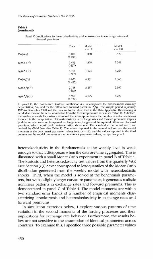
Panel C: Implications for heteroskedasticity and leptokurtosis in exchange rates and forward premiums

Data Model Model y = .2 y = 2.0

Ku(Asr) 3.000 (1.290)

,058 ,579

@ i ( ( A s ~ ) ~ ) 2.419 C.427)

1.368 2.541

~ ~ Z ( ( A S I ) ~ ) 4.101 C.717)

1.424 4.268

Ku(AfP0 8.635 4.331 6.363 (2.495)

Y ~ ( ( A ~ P O ~ ) 2.718 (.413)

3.257 2.397

v5z((Afpr)') 5.957 4 175 4.277 (1.174)

In panel C, the normalized kurtosis coefficient K u is computed for (de-meaned) currency depreciation, Asr,and for the differenced forward premium, A fpr . The sample period is January 1975 to December 1990 and the data are further described in the Data Appendix. Differencing is needed to remove the serial correlation from the forward premium series (see Table 1). As before, the symbol v stands for variance ratio and the subscript indicates the number of autocorrelations included in the computation. Heteroskedasticity in exchange rates and forward premiums implies positive serial correlation in squared exchange rate changes and the squared differenced forward premium, which would yield variance ratios above one. The standard errors in column 1 are derived by GMM (see also Table 1). The values reported in the second column are the model moments at the benchmark parameter values (with y = .2), and the values reported in the third column are the model moments at the benchmark parameter values, except that y = 2.

heteroskedasticity in the fundamentals at the weekly level is weak enough so that it disappears when the data are time aggregated. This is illustrated with a small Monte Carlo experiment in panel B of Table 4. The kurtosis and heteroskedasticity test values from the quarterly VAR (see Section 3.3)never correspond to low quantiles of the Monte Carlo distribution generated from the weekly model with heteroskedastic shocks. Third, when the model is solved at the benchmark parameters, but with a slightly larger curvature parameter, it generates realistic nonlinear patterns in exchange rates and forward premiums. This is demonstrated in panel C of Table 4. The model moments are within two standard error bands of a number of empirical moments char- acterizing leptokurtosis and heteroskedasticity in exchange rates and forward premiums.

In simulation exercises below, I explore various patterns of time variation in the second moments of the forcing processes and their implications for exchange rate behavior. Furthermore, the results below are not sensitive to the assumption of identical parameters across countries. To examine this, I specified three possible parameter values

Time Variatzvn cfRisk afzd Return

for ( 6 ,a): (.408, .236). (.80. .13), and (376, .071)-the latter parameters obtained from the data on weekly U.S. M1 growth rates. They imply 3* = 81 different parameter combinations for the heteroskedasticity in the four exogenous processes. The range of variation of the implied endogenous moments of interest over these 81 parameter combinations was quite small.

4. Simulation Results

4.1 Comparing different models Simulation results are reported for a CIA model, the transaction cost model with time-additive preferences, the transaction cost model with durability, the transaction cost model with durability and habit persistence, and finally for the complete model incorporating time-varying uncertainty in the fundamentals.

4.1.1 CIA model. Table 5, panel A contains simulations for the benchmark parameter values. Panel B increases the curvature parameter for the utility function to two. A CIA model with time-additive preferences and binding CIA constraints is a special case of our model when the velocities equal one. Expressions for and fp , in terms of the exogenous processes are given by

Y;- IAst+, = (y - 1) [ln % - In - - In 9,(25)x;' Y:

f p t = (Y - ~)EU?*- u:'l+ UZ- ur4+ v, (26)

where u j indicates the conditional mean of ln(j;+*/j:'), j = M , N, x,y, and v is a constant depending on the (co-) variances of the forcing processes. When y = 1 (log-utility), exchange rates only depend on money and are consequently highly persistent and not very variable. Likewise, forward premiums are very persistent and show considerable variance because future money supplies are highly predictable.

When y differs from 1, exchange rates also depend on the supply shocks, which are uncorrelated (see above). Therefore, their variability increases and their persistence drops, which is apparent from the second column in panels A and B. Clearly, the CIA model overpredicts the persistence of exchange rates and underpredicts its variability. The simple model implies realistic forward premium volatility and underpredicts its persistence at long horizons. As shown before [Bekaert (1994)1, the variability of the risk premium is negligible in CIA models.

The Retleui of Frnanctal Studzes / v 9 7.1 2 1996

Table 5 Simulation results for exchange rate changes and the forward premium

Panel A: Benchmark parameters ( y = .2)

Data CIA T.4TC DTC DHTC DHTC 6 , = 0 6 , = 0 6 , = 0 6, = 0 S,,, = ,408, S,, = .80 a,=O a,=O a ,=O a ,=O am,,=.236,a, ,=.13

Panel B: Benchmark parameters with y = 2

Data CIA TATC DTC DHTC DHTC 6 , = 0 6 , = 0 6 , = 0 6 , = 0 6,,,, =.408;6, ,=.80 a , = 0 a , = 0 a , = 0 a , = 0 a,,,, = ,236; = .13

6 ( A s t ) 17.668 4.159 7.544 7.541 12.650 13.840 (1.069)

g(fp,,4) 3,481 3.731 ,685 ,865 3.903 C.343)

( f ) 12.350 7.952 1.176 3.421 10.009 c.390)

4.1.2 Introducing transaction costs. Panel B best illustrates the effects of the different features of the model. The transaction cost technology induces variable velocities. Variable velocity both increases the variability of currency depreciation and dilutes the persistence that is injected by the highly autocorrelated money supply rules. However, it also implies less predictable IMRS, making their predictable parts- interest rates-less variable and less persistent.

Tinte Variationof Risk and Return

Table 5 (continued)

Panel C. Sensitivity analysis

Data EXTR CON MON MPU MPD

The first column of the table repeats the data moments reported in Table 1. The sample period is January 1975 to December 1990, Asr is the weekly logarithmic change in the dollar/pound exchange rate, and fpt is the forward premium, measured as the difference between the U.S. 1-month interest rate and the U.K. 1-month interest rate. A11 interest rates are annualized, that is, they are multiplied by 1,200. Weekly currency depreciation is also multiplied by 1,200. The symbol a always denotes the standard deviation, and v, stands for variance ratio, computed using i autocorrelations. The number between parentheses is a GMM-based standard error for the data moment.

The simulated sample used in computing the endogenous model moments has 4,000 observations Second-order polynomials are used in approximating the endogenous variables. The acronyms are understood as CIA = cash in advance, TC = transaction cost technology, TA = time additive. D = durability, DH = durability and habit persistence. The benchmark parameters for DHTC are B = .97'Ii2, rl = .75, 0 = .95, p = .76, c = ,090,6 = 2.5, y = 0.2. The first column repeats the data moments and their GMM-based standard errors. The next three columns of the table contain simpler variations of the benchmark specification, for example TATC in panel A denotes a time-additive model ( q = 0.0, f i = 0.0) with a transaction cost technology and addilog preferences with a curvature parameter equal to .2. The forcing processes are generated according to the estimated parameters of Table 3. Except for the Far-right column, there is no time variation in the second moments of the forcing processes. In the far-right column, the parameters E2 are specified as discussed in Table 4. For any simulation with conditional heteroskedasticity, polynomial elements with a higher than .99 correlation with other polynomial elements are discarded in order to reduce the dimensionality of the system.

Panel A reports results for the benchmark curvature parameter ( y = . 2 ) , whereas in panel B, y is set equal to 2. In panel C, the first column (EXTR) reports results for more extreme parameter values: y = 2.2; q = ,230; 0 = .98 but with the benchmark case conditional heteroskedasticity. Columns 2 through 5 examine the sensitivity to changes in the forcing process parameters. The other parameters are set equal to their benchmark values, except for y which is set equal to 2.0. In CON the variability of the consumption shocks is doubled relative to the benchmark parameters, keeping the correlations between the exogenous variables intact. In MON, analogously, the variability of the money shocks is doubled. In MPU (MPD), the autoregressive parameters are put equal to two standard errors above (below) the estimated value.

4.1.3 Introducing durability. Introducing durability potentially provides a remedy to this persistence puzzle. Suppose the agent ex- pects high home endowment growth. Because she desires to smooth consumption, she attempts to consume part of the bumper crop now.

l%e Recieu: of Financial Studies/ c. 9 n 2 1996

As she is constrained by her present income, she attempts to sell bonds which drives up interest rates. This makes her willing to buy her share of the current endowment. With durability, a positive shock builds into the service flows and is likely to cause a revision of expectations in the next period as well, hence injecting more persistence in interest rates. The high depreciation rate 1 - k,, and the lack of any correlation in the original endowment growth rates, reduce the potential impact of durability. Also note that the IMRS are just about as variable here as they were in the time-additive model, so that exchange rate variability is virtually unaffected.

4.1.4 Introducing habit persistence. The next column reports the results for the benchmark parameter configuration, but with Ez still set equal to zero. It offers the most satisfactory match with the data. The economic intuition behind the results is straightforward. With habit formation, consumers are more reluctant to diverge from smooth consumption streams. One could interpret the habit stock as a subsistence level from which it is very painful to deviate. This leads to more variable IMRS, exchange rates, and forward premiums: when the fundamentals change or expectations get revised, agents require larger price movements to hold the endowments. Although the model matches forward premium volatility, exchange rate variability is still somewhat too low.

This specification also comes close to explaining the persistence puzzle. The persistent service flows generated under this preference specification generate substantial persistence in endogenous interest rates, but the model still fails to deliver the persistence observed in forward premium data. On the other hand, the supply shocks cause a large enough forecast error in the IMRS to keep the persistence of exchange rates low. Strikingly, exchange rates show significant mean reversion at long hor i~ons . '~ This also results from long-run habit. A positive home supply shock weakens the dollar by reducing its marginal utility. The endowment adds to the stock of durables and hence affects the marginal utility of the dollar in the next period as well. Of course, new shocks mitigate this effect and keep the positive persistence at low levels. The higher service flow today also adds to the habit stock tomorrow; and the higher habit stock eventually increases the marginal utility of the dollar, causing the negative correlations. As expected, negative correlations start to dominate after 2 months.

When y is dropped to .2 in the benchmark case, all models per-

l 5 Huizinga (1987) finds evidence for mean reversion in realexchange rates

454

Rme Variation of Risk and Return

form dismally. They severely underpredict both the persistence and variability of exchange rate changes and forward premiums. Clearly. the utility function must have some curvature for habit persistence to generate significant effects.

4.1.5 Introducing time-varying uncertainty in the fundamentals. As both panels show, the model underpredicts the variance of the risk premium by several orders of magnitude. Although habit persistence slightly increases the standard deviation of the risk premium, the largest effects are observed under allowances for time-varying uncertainty in the forcing processes. Risk premium volatility is larger by a factor of about two (panel A) to over four (panel B), compared to the case without heteroskedasticity in the forcing processes. Time-varying uncertainty also increases the variability of both exchange rates and forward premiums. Still, even with y = 2 , risk premium variability in the data exceeds the model by more than 50 times.

Several conclusions can be drawn from the analysis of the various models:

1. Without some curvature in the utility function, even the rich- est model with variable velocities, nonseparable preferences, and time-varying uncertainty in the fundamentals fits poorly with the data. Nevertheless, the benchmark model fares better than previous models.

2. With risk aversion modestly higher than log-utility, however, the complete model performs relatively well with respect to the per-sistence puzzle, although it produces too much mean reversion in exchange rates and somewhat underpredicts the persistence of forward premiums. Simpler models either significantly underpredict the persistence of forward premiums or dramatically overpredict the persistence of exchange rates. The persistence of forward premiums derives primarily from the long-run habit persistence and is reduced when time-varying uncertainty in the fundamentals is allowed. This probably reflects the fact that IMRSs are less persistent with time-varying uncertainty.

3. All models fail drastically with respect to the volatility puzzle, pro-ducing a(Ast)> o ( fp,) > a (rp,) instead of a(Ast)> o(rpt)> a ( fp,). The model with time-varying uncertainty provides the best fit, matching exchange rate volatility and producing a much more variable risk premium. However, it slightly overpredicts forward premium volatility.

We now examine whether changing benchmark parameters brings the model closer to matching the variability of the risk premium without sacrificing performance with respect to the persistence puzzle.

f ie Reriieul of Fina?zcial Studies / v 9 n 2 1996

4.2 Risk, uncertainty, and exchange rates In this section, I explore the effect of different patterns of heteroskedasticity in the forcing processes on equilibrium exchange rate moments. I examine the importance of (i) the persistence of conditional variance shocks to the fundamentals and of (ii) the leptokurtic nature of the shocks. The former is governed by the coefficient on past variances in the GARCH specification; the latter is primarily governed by the coefficient on past residuals. In a first experiment, the kurtosis coefficients of the money processes are fixed at their benchmark values; and I vary 6 , = 6 , to generate a half-life of conditional variance shocks varying between 0.5 and 9 weeks. In a second experiment, I fix the persistence of conditional variance shocks (i.e., 6 , = .408), but I adapt a , = an to generate kurtosis coefficients varying between 0.01 and 6.0. The heteroskedasticity parameters for the consumption processes are set to maintain the ratio of the implied half-life (kurtosis) relative to the half-life (kurtosis) associated with the money parameters.

Figure 1displays the results for the variability of the risk premium. The three lines correspond to different choices for the curvature parameter, y ; the other parameters are set at their benchmark values. The full horizontal line represents the sample value, and the dot- ted horizontal lines are two standard error bands around the sample value.

At all three y values, increasing the exogenous kurtosis coefficient from 0.01 to 6.0 more than doubles the variability of the risk premium-although it only leads to modest increases in exchange rate and forward premium variability and it does not affect the persistence of the endogenous variables very much (not reported). Increasing the persistence of conditional variance shocks mainly increases the persistence of the forward premium while i: increases the variability of the risk premium by at most 60 percent.

To conclude, changes in the heteroskedasticity parameters bring us closer to resolving the variability puzzle, in that they primarily increase the variability of the risk premium. However, their effects are only substantial when combined with other nonlinear features in the model, such as strong risk aversion or habit persistence.

4.3 Sensitivity analysis Figure 2 shows the effect of changing the habit weight parameter, q, on the standard deviation of exchange rate changes, the forward premium, and the risk premium. The parameter q is varied between 0.3 and 0.85 for y = 2.0 and between 0.3 and 0.8 for y = 3.0. Again, the other parameters are fixed at their benchmark values.

The figure nicely illustrates the failure of the model to explain the volatility puzzle. The model can match the variability of all three vari-

Rme Variation of Risk and Return

A Effect d changes in half life of conditional variance shocb

0.5 0.75 1 2 3 4 5 0 7 8 9 half life [wnXrl

Effect of changes in kurtosis implied by conditional varlance shocb

Figure 1 Conditional heteroskedasticity in the fundamentals and the variability of the risk premium In both panels the horizontal lines indicate the sample moment for the variability of the risk premium and a two standard error band around it. Panel -4 explores the effect of changing the half-life of the conditional variance shocks onto the variability of the risk premium. The half-life varies between 0.5 and 9 weeks and the variability of the implied risk premium is graphed for three different values of the curvature parameter y . In panel B, a similar exercise is performed, hut now the kurtosis coefficient of the exogenous shocks is varied between .1and 6.0.

The Review of Financial Studze.~/ v 9 n 2 1996

Figure 2 Changesinthe habit weight parameter (q) and the variabjlity of the endogenous variables In all three panels the horizontal lines indicate the sample moment for the variability of, respecti\lely, exchange rate changes, the forward premium, and the risk premium, and a two standard error band around it. The habit weight parameter is varied between .3 and .85 for two choices of the curvature parameter y . The effects on the variability of exchange rate changes arc graphed in panel A, the effects on the variability of the forward premium are graphed in panel B, and the effects on the variability of the risk premium are graphed in panel C.


ables, including the risk premium, but not simultaneously.At y = 2.0, q = 0.85, it is true that the variability of the risk premium exceeds the variability of the forward premium as is true in the data. However, for these parameter values, the level of the variability of all three variables is too high.

Why does this occur? Recall that even a CIA model did a reasonable job in matching forward premium volatility. Increases in the habit weight parameter, as would increases in the curvature of the utility function, generally raise the level of nonlinearity in the model, thereby increasing the variability of IMRS. This, in turn, increases the variability of exchange rates and the risk premium. However, the variability of expected IMRS (interest rates) typically also goes up, which increases the variability of the forward premium. The model has no mechanism to limit the variability of expected IMRS while increasing the variability of IMRS per se. Moreover, the additional features introduced in this model affect the variability of the risk premium much more than the variability of either exchange rates or forward premiums, but in a sense they still affect the variability of exchange rates and forward premiums too much. This result parallels conclusions from single- country models that extreme habit persistence can match the equity premium, but at the expense of inducing implausible variability in the short interest rate.

The effect of more habit persistence is minimal in the benchmark case, for there is not enough curvature in the utility function. Increas- ing the habit weight also has ambiguous effects on the persistence puzzle. Forward premium persistence mostly goes up, but the model generates more mean reversion in exchange rates.

Table 5, panel C reports some additional sensitivity analysis. EXTR is another example of a parameter configuration for which the standard deviation of the risk premium is near two standard errors of the sample standard deviation. The curvature parameter is only 2.2, but the favorable effects are induced by increasing the long memory in the service flows through increasing 8 and by increasing the habit weight. Unfortunately, exchange rates and forward premiums are far too variable.

Panel C also reports simulations resulting from changing the forcing process parameters, respectively doubling the variability of the consumption shocks, doubling the variability of the money shocks, and increasing and decreasing the persistence of the money processes. Strikingly, the main conclusions remain valid. Exchange rate volatility is roughly matched but forward premium volatility is overpredicted by the model. Although performing much better than Backus, Gre- gory, and Telmer (1993), the model underpredicts the persistence of forward premiums and exchange rates. Finally, changes in consump-

The Review ofFinancia1Studies/v 9 n 2 I996

tion variability have the largest effect on the variability of the risk premium, but the variability reached in the data remains elusive.

The failure of the model to generate sufficient risk premium volatility also surfaces in the correlations between future spot changes and the current forward premium. Not a single experiment in all my simulations yields negative correlations!

5. Conclusions

Standard frictionless monetary general equilibrium models fail to explain the relative variability and persistence of exchange rates and the forward premium. They also fail to generate sufficient variation in the forward market risk premium. In this article, I maintained a frictionless rational expectations model but introduced a more realistic decision interval for the representative agents and more realistic preferences incorporating various forms of time nonseparabilities. The combination of time-varying uncertainty in the fundamentals and time aggregation was shown to be an important factor in explaining the risk premium puzzle. Simulation results indicated that the risk premium can be made several orders of magnitude more variable than in previous models without implying negatively autocorrelated forward premiums. Still, the model tends to overpredict the variability of the forward premium and to severely underpredict the variability of the risk premium.

Several generalizations of the present model are potentially useful. For example, Bekaert, Hodrick, and Marshall (1994) explore the pre- dictability of asset returns, including forward market returns, in a re- cursive preference framework with first-order risk aversion. Although first-order risk aversion also substantially increases the variance of the risk premium relative to time-additive models, the model substantially underpredicts the variability of exchange rates, the forward premium, and the risk premium.

The empirical results of Bekaert and Hodrick (1993) suggest another useful direction for further research. In an empirical reexamina- tion of the unbiasedness hypothesis, we find that unbiasedness holds for the British pound during the 1975 to 1980 period. In fact, the slope coefficient in a typical unbiasedness regression test is slightly larger than one for that subperiod. In the turbulent 1980s, the rejection of unbiasedness is very severe. Interestingly, for the 1973 to 1976 period, that is, before formal implementation of the floating exchange rate system, we also find negative slope coefficients. Rational agents, faced with an array of policy signals, may need time to recognize or "believe" changes in policy regimes. Such rational "learning" can lead to systematic forecast errors [Lewis (1989)l and partially explain the

Time Variation oJ'Risk and Return

negative slope coefficients. Moreover, policy regime switches may be one mechanism behind time-varying uncertainty in the fundamentals.

A third generalization is to break the complete markets setup. In that case, the IMRS need not be equalized across countries. As agents can still self-insure through asset trading, asset prices might not differ very much from the complete market case. However, the perfect risk sharing assumed in this article has several counterfactual implications. First of all, the extent of international portfolio diversification is actually very limited. Second, the setup implicitly imposes purchasing power parity (PPP), which is grossly violated in the data. In fact, when PPP deviations exist, investors in different countries measure their real returns differently and generally desire to hold different portfolios [Adler and Dumas (1983)l. An additional channel to break PPP is to explicitly model nontradables. When utility is nonseparable in tradables and nontradables, the IMRSs that are used to discount asset payoffs depend on nontradables as well. Lastly, the large current account imbalances between major industrial countries indicate the usefulness of a general equilibrium model that allows wealth redistributions. I intend to explore a heterogeneous agent economy with nontradable goods in the near future.

Appendix 1: Data

The exchange rate data are daily data from Citicorp Data Services from 1975 to the end of 1990. Robert Korajzyck supplied DRI Eurocurrency interest rates running until mid-1988 which were obtained at INSEAD. They were updated using data from Citicorp Data Services. All rates are sampled each Friday and are average bid and ask rates. When Friday was a holiday, the Thursday rate was used.

Matching the exchange rate sample period, the consumption and money data extend from the first quarter of 1975 to the final quarter of 1990. Quarterly consumption on nondurables and services is taken from the OECD Quarterly National Accounts. The U.K. semidurables category is included as it is comprised of consumption items that are included in the nondurables category for the United States. The series are seasonally adjusted and in 1982 dollars and 1985 pounds, respectively.

Money is measured as end of the quarter M2 money stocks. For the US., M2 is taken from Citibase. Due to the introduction of MMDAs and super-NOW accounts, there is an outlier in the U.S. data in the first quarter of 1983. The money growth rate for that quarter is replaced with a weighted average of past and future growth rates, incorporating 18 quarters of data. Published monetary aggregates in the U.K. cannot be used as there were several definitional changes that make

it virtually impossible to deduce a consistently defined series over the whole sample. Therefore, I obtained data on the concept M4 directly from the Bank of England. M4 is a broad aggregate comparable to M2 in the US., except that it also includes deposits (including certificates of deposit) with building societies. In November 1981, a big financial institution (the trustees savings bank) turned into a bank, increasing the money supply by 7.5 percent overnight (see Bank of England Quarterly Bulletin, December 1981). This outlier was corrected for in a similar fashion as the U.S. outlier. The money series are also seasonally adjusted. Both the money and real consumption data were divided by total population (series 992 in the International Financial Statistics data set) to arrive at per capita data. The population data are midyear estimates that are linearly interpolated to obtain quarterly data.

Appendix 2: The Calibration of S2,

In the nonstochastic steady state of the model, the expressions for velocity and interest rates only depend on the parameters in i l l . With addilog utility, steady-state home consumption velocity is given by

with upper bars denoting steady-state values. Likewise, the 4-week, steady-state interest rate is defined by

Total transaction costs as a proportion of total consumption, TC,, in steady state are given by

TC, = c,( ?X)cy-l . (A.3)

The expressions for the foreign good are similar. To obtain empirical estimates of the steady-state values, I compute

monthly interest rate means from the interest rate data used in this article and quarterly velocity means from the OECD data on consumption and consumption deflators and the money supply data described in the Data Appendix. To link quarterly (Vq) and weekly (V,) velocity, I assume

Rnze 17ariatto?zof Risk attd Return

An analogous expression holds for foreign consumption velocity. I consider the following parameter range:

To find a "reasonable" parameter configuration for f i l , the following procedure is performed:

1. Compute mean growth rates of home and foreign consumption and money from the simulated observations according to the law of motion specified in Equations (19) and (21) in the text. Set 6, equal to its estimated values, but set Z2 equal to zero.

2. For each parameter configuration, compute the steady states for velocity, the monthly interest rates, and transaction costs, TC, and TCY,using Equations (A.1) through (A.3).

3. Discard parameter configurations that yield TC, or TC, > .O1 and < .0001.

4. Discard parameter configurations that yield excessive or insuffi- cient velocity. The lower bound is computed as the weekly equivalent from the quarterly mean, computed with the data used in this article. As I used a broad monetary aggregate, I consider these means to overestimate the mean of velocity consistent with the transaction cost technology modeled in this article. I also compute an "adjusted" mean by multiplying all the velocities with the ratio of consumption to GNP as in Marshall (1992). 1 use this quartcAy mean as the upper bound for weekly velocities. Hence, the velocity mean requirements are weak.

5. Of the remaining parameter configurations, those parameters are chosen that most closely match the interest rate means. The resulting parameter configuration is nearly within a three standard error band of the data means. %'hen the curvature parameter is increased to 2.0, the parameter configuration still satisfies Condi- tions 3 and 4, but the interest rate means are somewhat higher than for the benchmark parameters.

Appendix 3: Solving the Model

As indicated in the text, the marginal utilities nzuxt and mu%, and the consumption velocities yxand P;' must be determined. The expression for mux, follows from Equations (12) and (13) in the text. It can

Tbe Revieu? of Financial Studies/ v 9 ?z 2 1996

be rewritten as

mux, = wl dmux, + hmuxt

A remaining problem is that, consistent with what is observed, the endowments and money supplies are assumed to grow over time. Therefore, I solve for a statiotzay equilibrium, in which stationary endogenous variables such as exchange rate changes, inflation, and velocity depend only on stationary state variables, including growth rates of money supplies and endowments. To induce stationarity in the stocks of consumption goods and the habit stocks, I divide by the level of consumption. This normalization is used by Heaton (1995) and leads to a natural stationary representation of the state vector. Define a scaled marginal utility as

mux, smux, = ---a ~ ( x i ' . 'vil)

where the denominator is the particular period utility function evaluated at present equilibrium consumption purchases. Define sdmuxt analogously by replacing muxt in Equation (A.6) by dmuxt. Then sdmuxt solves the following difference equation:

aucqt,,') aS;

sdmux, = ---a u(x;',Y:')

ax;'

An analogous equation applies to hmux,. Once market clearing is imposed, the marginal utility ratios in Equation (A.7) will be direct functions of the state vector and the difference equation can be solved for sdmux,. Note that smux, = wlsdmuxt + wshmux,. With the solution for smuxt, the Euler equation determining velocity can be

Time Variation of'Risk and Rettrrn

rewritten in stationary format:

As the right-hand side depends on state variables at time t , Equa-tion (A.8) describes the solution for a$x/ax and hence for velocity.

Let Ot E R~ be the vector of stationary-state variables that com- pletely spans the information set and rpt = I &X, v;', smziytl,S ~ Z I X ~ ,

the set of endogenous variables to be derived. The other endogenous variables are trivial functions of pt . As the model is dichotomous in p: = [vv,[V:, smuxt1 and rp{= smuytl, I can restrict the discussion to the solution method for p;. The two basic Euler equations that must be solved in this model are Equations (A.7) and (A.8). They are of the form

where A(. , .) and r ( . , .) are known functions. As vt is a continuous function mapping R ~ , itthe space of the state variables Ot, into R, can be approximated by polynomials. The polynomial coefficients are found by minimizing the approximation error over some norm. My technique follows Heaton (1995) in employing Monte Carlo integration to evaluate expectations.

More specifically, I first solve for the scaled marginal utilities. Let @,(Of)be a vector of polynomial elements in Ot of degree 5 n. De-note fn(Ot; qn) = [P,(ln(O,))'q,I), where q, indicates the polynomial coefficients. Let sdmuxt x f,(Ot; 9,). Substitute this in Equation (A.8) to find the approximation error u(Ot;9,):

The parameters q, are chosen such as to make u(Ot, q,) orthogonal

The Reuiezc of Financial Studies/ u 9 n 2 1996

to the polynomial elements p ( 0t , q,)16 or

(A.11)

By the law of iterated expectations, this can be rewritten as

The expectation can be taken by Monte Carlo integration, that is, by drawing a long time series for Ot and taking sample averages of the expression in Equation (A.12). The coefficients qn then follow from solving a system of nonlinear equations. The difference equation for shmuxt is solved analogously and smuxt is obtained as in Equation (A.5).

To solve for velocity, approximate 4"by polynomials and substitute the approximate velocity function into Equation (A.8). In this case, the polynomials will be exponentiated to guarantee positive velocities. The marginal utility smuxt is replaced by its previously derived approximation. This gives an approximation error that is projected onto the polynomial elements in order to solve for the polynomial coefficients.l7

Appendix 4: The Risk Premium Under Log-Normality

From Equations (6) and (7) in the text, exchange rate changes are the ratio of the foreign to home IMRS, whereas the forward premium is the log of the ratio of expected foreign IMRS to the expected home IMRS. Assume that mrst+4,,i,and r n r ~ ; + ~ , ~are jointly lognormally dis- tributed with ut, u: the respective conditional means and c,,c~: the respective conditional variances. Recall the logarithmic definition of the risk premium, rpt = Et[st+4- st]-fPrIt is then straightforward to derive

'"his is the Galerkin method, one of the minimum weighted residuals methods. described by Judd (1992).

"It is straightforward to compute analytical derivatives for the various nonlinear systems so that solutions are obtained relatively fast even for large state spaces.

llme I'uriation ofRisk and Return

As a special case, consider the following simple parameterization of the IMRS in the context of the Lucas (1982) model. In this CIA model, the dollar IMRS is given by

a ~ J ( X ~ + ~ ,Y , + J as,, , nt+4

m74t4.4 = a l r ( X , , n ) (A. 14) nta.G

where nt is the purchasing power of the dollar, xt is the amount of the home good, and yt is the amount of the foreign good purchased in equilibrium.

Assume a simple utility function that is separable in the two goods and where the coefficient of relative risk aversion with respect to both goods is y . Also assume that the CIA constraints are binding, as they are in Lucas's framework when interest rates are positive. In this case, the purchasing powers in equilibrium are just the ratios of output to money. Then the risk premium can be derived as

where ill (N) refers to the home (foreign) money supply, x (31)to home (foreign) consumption, and atdenotes the conditional (co)variance. The conditional moments apply to C:=(=, ln(Azt+,) for z = x, y, ibf.S. The first bracketed term reflects consumption risk: the second, purchasing power (nominal) risk; and the third term, the interaction of the two.18 This expression immediately reveals the importance of allowing for time-varying uncertainty in the fundamentals.

Furthermore, suppose that the innovations to ( rn r .~~+4,~ , my$+ ,.4) are normal with a variance-covariance matrix that changes over time according to a GARCH model. This implies that third moments of the innovations are zero. [Jnder that same assumption, it follows

This is inconsistent with the implication of a typical unbiasedness test:

This explains the etllpirical failure of Kanlinsky and Peruga (1990)

'"ngel (1992) stresses the impnltance of covariances between market fundamentals in the context of this model; nevertheless, both Canova and hlarrinan (1993) and Hodrick (1989) ignore them.

467

7be Review of Financial Studies / 0 9n 2 I9G

who relied on a lognormal CIA model to generate time variation in the foreign exchange risk premium. My model avoids these implications for the risk premium through two channels: the transaction cost technology and the temporal dependencies in preferences.

References Abel, A. B., 1988, "Stock Prices under Time-varying Dividend Risk: An Exact Solution in an Infinite Horizon General Equilibrium Model," Journal ofMonetary Economics, 22, 375-394.

Adler. M., and B. Dumas, 1983, "International Portfolio Choice and Corporation Finance," Journal of Finance, 38. 925-984.

Andrews. D. K.. 1991. "Heteroskedasticity and Autocorrelation Consistent Covariance Matrix Estimation." Econometrica,59, 817-858.

Backus. D., A. Gregory, and C Telmer. 1993, "Accounting for Forward Rates in Markets for Foreign Currency,"JournalofFtnance, 5, 1887-1908.

Baillie, R.. and T. Bollerslev. 1989. "The Message in Daily Exchange Rates: A Conditional Variance Tale." Journal of Business and Economic Statistics, 7. 297-305.

Bansal, R., A. R. Gallant. R. Hussey, and G. Tauchen, 1995, "Nonparametric Estimation of Structural Models for High-Frequency Currency Market Data." Journal ofEconometrics. 66. 251-287.

Bekaert. G., 1992. "Empirical Analyses of Foreign Exchange Markets: General Equilibrium Perspectives." Ph.D, dissenation. Northwestern Llniversity.

Bekaert, G.. 1994. "Exchange Rate Volatility and Deviations from Unbiasedness in a Cash-in- Advance Model." Journal of International Economics, 36. 29-52.

Bekaert, G., 1995. "The Time-variation of Expected Returns and Volatility in Foreign Exchange Markets,"Journal of Business and Economic Statistics, 13. 397408.

Bekaert, G.. and R. Hodrick, 1993, "On Biases in the Measurement of Foreign Exchange Risk Premiums,"Journal of International Money and Finance, 12. 115-138.

Bekaert, G., R. Hodrick. and D. Marshall. 1994. "The Implications of First-Order Risk Aversion for Asset Market Risk Premiums," working paper. Northwestern and Stanford University.

Bera. A. K . , and C. M. Jarque. 1982, "Model Specification Tests: A Simultaneous Approach. Journal of Econometrics, 20, 59-82.

Bollerslev. T., 1990. "hlodeling the Coherence in Short Run Nominal Exchange Rates: A Multivariate Generalized ARCH Model," Revfeu' of Economics and Statistics. 72. 498-505.

Bollerslev. T., R. Y. Chou. and K. F. Kroner, 1992, "ARCH Modelling in Finance: A Review of the Theory and Empirical Evidence." Journal of Econometrics, 52, 5 4 0 .

Canova, F,, and J. Marrinan. 1993, "Profits. Risk and Uncertainty in Foreign Exchange Markets." Journal ofMonetary Economics. 32. 259-286.

Constantinides. G. M.. 1990. "Habit Formation: A Resolution of the Equity Premium Puzzle," Journal ofPolitica1 Economy, 98. 519-543.

Cumby. R. E., and J. Huizinga, 1992, "Testing the Autocorrelation Structure of Disturbances in Ordinary Least Squares and Instrumental Variables Regressions." Econometrica. 60. 185-196.

Diebold. F. X., 1986, "Temporal Aggregation of ARCH Models and the Distribution of Asset Returns," working paper. University of Pennsylvania.


Drost, E C., and T. E. Nijman. 1993. "Temporal Aggregation of GARCH Processes." Econometrica, 61. 909-928.

Dunn, K. B., and K. J . Singleton. 1986, "Modelling the Term Structure of Interest Rates under Non- separable Utility and Durability of Goods" Journal ofFinancia1 Economics. 17. 27-55.

Eichenbaum, M. S . , and L. P. Hansen. 1990, "Estimating Models with Intertemporal Substitution Using Aggregate Time Series Data," Journal of Business and Economic Statistics. 8. 53-69.

Eichenbaum, M. S., L. P. Hansen, and K. J. Singleton, 1988, "A Time Series Analysis of a Representative Agent hlodel of Consumption and Leisure Choice under Uncertainty." Qua?terly Journal ofEconomics. 103, 51-78.

Engel, C.. 1992, "On the Foreign Exchange Risk Premium in a General Equilibrium Model," Journal of Inter?zational Eco?zomics. 32. 305-319.

Engle, R.. 1982. "Autoregressive Conditional Heteroskedasticity w-ith Estimates of the Variance of U.K. Inflation." Econometn'ca.50, 987-1008.

Ferson. W., and G. M. Constantinides, 1991, "Habit Persistence and Durability in Aggregate Consumption: Empirical Tests." Journal ofAnancia1 Economics. 29, 199-240.

Hall, R. E., 1988, "Intertemporal Substitution in Consumption," Journal ofPolitica1 Economy, 96. 339-357.

Hansen. L. P., 1982, "Large Sample Properties of Generalized hlethod of Moments Estimators." Econometrica,50, 1029-1054.

Hansen, L. P., and R. Jagannathan, 1991, "Implications of Security Market Data for Models of Dynamic Economies," Journal of Political Economy, 99, 225-262.

Hansen, L. P., and T. J. Sargent, 1983, "The Dimensionality of the Aliasing Problem in Models with Rational Spectral Densities," Econometrica, 51, 377-388.

Heaton, J.. 1995. "An Empirical Investigation of Asset Pricing with Temporally Dependent Preference Specifications." working paper. Massachusetts Institute of Technology, forthcoming in Econometrica.

Hodrick. R J.. 1989. "Risk. Uncertainty and Exchange Rates," Journal ofMonetay Economics, 23. 4 3 H 6 0 .

Hodrick. R., N. Kocherlakota. and D. Lucas, 1991. "The Variability of Velocity in Cash-in-Advance hlodels," Journal ofPolitica1 Economy, 99, 358-384.

Huizinga, J., 1987. "An Empirical Investigation of the Long-run Behavior of Real Exchange Rates." Carizegie-Rochester Copference Series on Pt4blic Policy. 27, 149-21 4.

Judd, K. L.. 1992, "Projection Methods for Solving Aggregate Growth blodels." Jourizal ofEconomic 7heoy. 58. 410-452.

Kaminsky, G., and R. Peruga, 1990, "Can a Time-Varying Risk Premium Explain Excess Returns in the Forward Market for Foreign Exchange?" Journal ofIntematio?zalEconottzics,28. 47-70.

Lewis, K.. 1989. "Changing Beliefs and Systematic Rational Forecast Errors with Evidence from Foreign Exchange." American Economic Reviezq 79. 621-636.

Lucas. D.. 1994. "Asset Pricing with Undiversifiable Income Risk and Short Sales Constraints: Deepening the Equity Premium Puzzle," Journal ofMonetaty Economics. 34. 325-341.

Lucas. R. E., 1978. "Asset Prices in an Exchange Economy," Econotnetrica, 46. 1429-1445.

The Ketlzew of Financial Studies// 9 n 2 2996

Lucas, R. E., 1982, "Interest Rates and Currency Prices in a Two-Country World," Journal oj Monetay Ecoriomics. 10. 335-360.

Marcet. A,, and D. Marshall, 1993, "Convergence of Approximate Model Solutions to Rational Expectations Equilibria Using the Method of Parameterized Expectations." working paper. Northwestern University.

~Marcet, A,. and K. J. Singleton. 1990. "Optimal Consumption-Savings Decisions and Equilibrium Asset Prices with Heterogeneous Agents Subject to Portfolio Constraints, working paper. Stanford University.

Marshall, D.. 1992, "Inflation and Asset Returns in a Monetary Economy," JourtzalofFinance. 47, 1315-1342.

Meese, R., 1990, "Currency Fluctuations in the Post-Bretton K'oods Area," Journal of Economic Perspecti~,es.4 , 117-134.

Newey. W., and K. West. 1987, "A Simple, Positive Semi-definite, Heteroskedasticity and Autocorrelation Consistent Covariance Matrix." Econometrica.55. 703-708.

Nijman. T. E.. and F. C. Palm. 1990. "Parameter Identification in ARMA Processes in the Presence of Regular but Incomplete Sampling." Journal of Time Series Analysis, 11. 239-248.

Sundaresan. S. M., 1989. "Intertemporally Dependent Preferences and the Volatility of Consumption and Wealth," Review of Financial Studies. 2. 73-89.

Svensson. L. . 1985. "Currency Prices. Terms of Trade and Interest Rates: A General Equilibrium Asset Pricing Cash-in-Advance Approach." Journal oflnternational Ecor~omics. 18, 17-41,

Telmer, C. I., 1993, "Asset-Pricing Puzzles and Incomplete Markets,"./ournal ofFinance, 48, 1 8 0 5 1832.

Working, H., 1960, "Note on the Correlation of First Differences of Averages in a Random Chain," Econometrica,28, 916918.

You have printed the following article:

The Time Variation of Risk and Return in Foreign Exchange Markets: A GeneralEquilibrium PerspectiveGeert BekaertThe Review of Financial Studies, Vol. 9, No. 2. (Summer, 1996), pp. 427-470.Stable URL:


This article references the following linked citations. If you are trying to access articles from anoff-campus location, you may be required to first logon via your library web site to access JSTOR. Pleasevisit your library's website or contact a librarian to learn about options for remote access to JSTOR.

[Footnotes]

1 The Time Variation of Expected Returns and Volatility in Foreign-Exchange MarketsGeert BekaertJournal of Business & Economic Statistics, Vol. 13, No. 4. (Oct., 1995), pp. 397-408.Stable URL:

http://links.jstor.org/sici?sici=0735-0015%28199510%2913%3A4%3C397%3ATTVOER%3E2.0.CO%3B2-C

5 Large Sample Properties of Generalized Method of Moments EstimatorsLars Peter HansenEconometrica, Vol. 50, No. 4. (Jul., 1982), pp. 1029-1054.Stable URL:

http://links.jstor.org/sici?sici=0012-9682%28198207%2950%3A4%3C1029%3ALSPOGM%3E2.0.CO%3B2-O

6 Asset-Pricing Puzzles and Incomplete MarketsChris I. TelmerThe Journal of Finance, Vol. 48, No. 5. (Dec., 1993), pp. 1803-1832.Stable URL:

http://links.jstor.org/sici?sici=0022-1082%28199312%2948%3A5%3C1803%3AAPAIM%3E2.0.CO%3B2-5

9 Habit Formation: A Resolution of the Equity Premium PuzzleGeorge M. ConstantinidesThe Journal of Political Economy, Vol. 98, No. 3. (Jun., 1990), pp. 519-543.Stable URL:

http://links.jstor.org/sici?sici=0022-3808%28199006%2998%3A3%3C519%3AHFAROT%3E2.0.CO%3B2-T

http://www.jstor.org

LINKED CITATIONS- Page 1 of 6 -

NOTE: The reference numbering from the original has been maintained in this citation list.

http://links.jstor.org/sici?sici=0893-9454%28199622%299%3A2%3C427%3ATTVORA%3E2.0.CO%3B2-5&origin=JSTOR-pdf

http://links.jstor.org/sici?sici=0735-0015%28199510%2913%3A4%3C397%3ATTVOER%3E2.0.CO%3B2-C&origin=JSTOR-pdf

http://links.jstor.org/sici?sici=0012-9682%28198207%2950%3A4%3C1029%3ALSPOGM%3E2.0.CO%3B2-O&origin=JSTOR-pdf

http://links.jstor.org/sici?sici=0022-1082%28199312%2948%3A5%3C1803%3AAPAIM%3E2.0.CO%3B2-5&origin=JSTOR-pdf

http://links.jstor.org/sici?sici=0022-3808%28199006%2998%3A3%3C519%3AHFAROT%3E2.0.CO%3B2-T&origin=JSTOR-pdf

References

International Portfolio Choice and Corporation Finance: A SynthesisMichael Adler; Bernard DumasThe Journal of Finance, Vol. 38, No. 3. (Jun., 1983), pp. 925-984.Stable URL:

http://links.jstor.org/sici?sici=0022-1082%28198306%2938%3A3%3C925%3AIPCACF%3E2.0.CO%3B2-U

Heteroskedasticity and Autocorrelation Consistent Covariance Matrix EstimationDonald W. K. AndrewsEconometrica, Vol. 59, No. 3. (May, 1991), pp. 817-858.Stable URL:

http://links.jstor.org/sici?sici=0012-9682%28199105%2959%3A3%3C817%3AHAACCM%3E2.0.CO%3B2-P

Accounting for Forward Rates in Markets for Foreign CurrencyDavid K. Backus; Allan W. Gregory; Chris I. TelmerThe Journal of Finance, Vol. 48, No. 5. (Dec., 1993), pp. 1887-1908.Stable URL:

http://links.jstor.org/sici?sici=0022-1082%28199312%2948%3A5%3C1887%3AAFFRIM%3E2.0.CO%3B2-7

The Message in Daily Exchange Rates: A Conditional-Variance TaleRichard T. Baillie; Tim BollerslevJournal of Business & Economic Statistics, Vol. 7, No. 3. (Jul., 1989), pp. 297-305.Stable URL:

http://links.jstor.org/sici?sici=0735-0015%28198907%297%3A3%3C297%3ATMIDER%3E2.0.CO%3B2-J

The Time Variation of Expected Returns and Volatility in Foreign-Exchange MarketsGeert BekaertJournal of Business & Economic Statistics, Vol. 13, No. 4. (Oct., 1995), pp. 397-408.Stable URL:

http://links.jstor.org/sici?sici=0735-0015%28199510%2913%3A4%3C397%3ATTVOER%3E2.0.CO%3B2-C




http://links.jstor.org/sici?sici=0022-1082%28198306%2938%3A3%3C925%3AIPCACF%3E2.0.CO%3B2-U&origin=JSTOR-pdf

http://links.jstor.org/sici?sici=0012-9682%28199105%2959%3A3%3C817%3AHAACCM%3E2.0.CO%3B2-P&origin=JSTOR-pdf

http://links.jstor.org/sici?sici=0022-1082%28199312%2948%3A5%3C1887%3AAFFRIM%3E2.0.CO%3B2-7&origin=JSTOR-pdf

http://links.jstor.org/sici?sici=0735-0015%28198907%297%3A3%3C297%3ATMIDER%3E2.0.CO%3B2-J&origin=JSTOR-pdf

http://links.jstor.org/sici?sici=0735-0015%28199510%2913%3A4%3C397%3ATTVOER%3E2.0.CO%3B2-C&origin=JSTOR-pdf

Modelling the Coherence in Short-Run Nominal Exchange Rates: A Multivariate GeneralizedArch ModelTim BollerslevThe Review of Economics and Statistics, Vol. 72, No. 3. (Aug., 1990), pp. 498-505.Stable URL:

http://links.jstor.org/sici?sici=0034-6535%28199008%2972%3A3%3C498%3AMTCISN%3E2.0.CO%3B2-N

Habit Formation: A Resolution of the Equity Premium PuzzleGeorge M. ConstantinidesThe Journal of Political Economy, Vol. 98, No. 3. (Jun., 1990), pp. 519-543.Stable URL:

http://links.jstor.org/sici?sici=0022-3808%28199006%2998%3A3%3C519%3AHFAROT%3E2.0.CO%3B2-T

Testing the Autocorrelation Structure of Disturbances in Ordinary Least Squares andInstrumental Variables RegressionsRobert E. Cumby; John HuizingaEconometrica, Vol. 60, No. 1. (Jan., 1992), pp. 185-195.Stable URL:

http://links.jstor.org/sici?sici=0012-9682%28199201%2960%3A1%3C185%3ATTASOD%3E2.0.CO%3B2-2

Temporal Aggregation of Garch ProcessesFeike C. Drost; Theo E. NijmanEconometrica, Vol. 61, No. 4. (Jul., 1993), pp. 909-927.Stable URL:

http://links.jstor.org/sici?sici=0012-9682%28199307%2961%3A4%3C909%3ATAOGP%3E2.0.CO%3B2-2

Estimating Models with Intertemporal Substitution Using Aggregate Time Series DataMartin Eichenbaum; Lars Peter HansenJournal of Business & Economic Statistics, Vol. 8, No. 1. (Jan., 1990), pp. 53-69.Stable URL:

http://links.jstor.org/sici?sici=0735-0015%28199001%298%3A1%3C53%3AEMWISU%3E2.0.CO%3B2-G

A Time Series Analysis of Representative Agent Models of Consumption and Leisure Choiceunder UncertaintyMartin S. Eichenbaum; Lars Peter Hansen; Kenneth J. SingletonThe Quarterly Journal of Economics, Vol. 103, No. 1. (Feb., 1988), pp. 51-78.Stable URL:

http://links.jstor.org/sici?sici=0033-5533%28198802%29103%3A1%3C51%3AATSAOR%3E2.0.CO%3B2-V




http://links.jstor.org/sici?sici=0034-6535%28199008%2972%3A3%3C498%3AMTCISN%3E2.0.CO%3B2-N&origin=JSTOR-pdf

http://links.jstor.org/sici?sici=0022-3808%28199006%2998%3A3%3C519%3AHFAROT%3E2.0.CO%3B2-T&origin=JSTOR-pdf

http://links.jstor.org/sici?sici=0012-9682%28199201%2960%3A1%3C185%3ATTASOD%3E2.0.CO%3B2-2&origin=JSTOR-pdf

http://links.jstor.org/sici?sici=0012-9682%28199307%2961%3A4%3C909%3ATAOGP%3E2.0.CO%3B2-2&origin=JSTOR-pdf

http://links.jstor.org/sici?sici=0735-0015%28199001%298%3A1%3C53%3AEMWISU%3E2.0.CO%3B2-G&origin=JSTOR-pdf

http://links.jstor.org/sici?sici=0033-5533%28198802%29103%3A1%3C51%3AATSAOR%3E2.0.CO%3B2-V&origin=JSTOR-pdf

Autoregressive Conditional Heteroscedasticity with Estimates of the Variance of UnitedKingdom InflationRobert F. EngleEconometrica, Vol. 50, No. 4. (Jul., 1982), pp. 987-1007.Stable URL:

http://links.jstor.org/sici?sici=0012-9682%28198207%2950%3A4%3C987%3AACHWEO%3E2.0.CO%3B2-3

Intertemporal Substitution in ConsumptionRobert E. HallThe Journal of Political Economy, Vol. 96, No. 2. (Apr., 1988), pp. 339-357.Stable URL:

http://links.jstor.org/sici?sici=0022-3808%28198804%2996%3A2%3C339%3AISIC%3E2.0.CO%3B2-8

Large Sample Properties of Generalized Method of Moments EstimatorsLars Peter HansenEconometrica, Vol. 50, No. 4. (Jul., 1982), pp. 1029-1054.Stable URL:

http://links.jstor.org/sici?sici=0012-9682%28198207%2950%3A4%3C1029%3ALSPOGM%3E2.0.CO%3B2-O

Implications of Security Market Data for Models of Dynamic EconomiesLars Peter Hansen; Ravi JagannathanThe Journal of Political Economy, Vol. 99, No. 2. (Apr., 1991), pp. 225-262.Stable URL:

http://links.jstor.org/sici?sici=0022-3808%28199104%2999%3A2%3C225%3AIOSMDF%3E2.0.CO%3B2-L

The Dimensionality of the Aliasing Problem in Models with Rational Spectral DensitiesLars Peter Hansen; Thomas J. SargentEconometrica, Vol. 51, No. 2. (Mar., 1983), pp. 377-387.Stable URL:

http://links.jstor.org/sici?sici=0012-9682%28198303%2951%3A2%3C377%3ATDOTAP%3E2.0.CO%3B2-3

The Variability of Velocity in Cash-in-Advance ModelsRobert J. Hodrick; Narayana Kocherlakota; Deborah LucasThe Journal of Political Economy, Vol. 99, No. 2. (Apr., 1991), pp. 358-384.Stable URL:

http://links.jstor.org/sici?sici=0022-3808%28199104%2999%3A2%3C358%3ATVOVIC%3E2.0.CO%3B2-V




http://links.jstor.org/sici?sici=0012-9682%28198207%2950%3A4%3C987%3AACHWEO%3E2.0.CO%3B2-3&origin=JSTOR-pdf

http://links.jstor.org/sici?sici=0022-3808%28198804%2996%3A2%3C339%3AISIC%3E2.0.CO%3B2-8&origin=JSTOR-pdf

http://links.jstor.org/sici?sici=0012-9682%28198207%2950%3A4%3C1029%3ALSPOGM%3E2.0.CO%3B2-O&origin=JSTOR-pdf

http://links.jstor.org/sici?sici=0022-3808%28199104%2999%3A2%3C225%3AIOSMDF%3E2.0.CO%3B2-L&origin=JSTOR-pdf

http://links.jstor.org/sici?sici=0012-9682%28198303%2951%3A2%3C377%3ATDOTAP%3E2.0.CO%3B2-3&origin=JSTOR-pdf

http://links.jstor.org/sici?sici=0022-3808%28199104%2999%3A2%3C358%3ATVOVIC%3E2.0.CO%3B2-V&origin=JSTOR-pdf

Changing Beliefs and Systematic Rational Forecast Errors with Evidence from ForeignExchangeKaren K. LewisThe American Economic Review, Vol. 79, No. 4. (Sep., 1989), pp. 621-636.Stable URL:

http://links.jstor.org/sici?sici=0002-8282%28198909%2979%3A4%3C621%3ACBASRF%3E2.0.CO%3B2-U

Asset Prices in an Exchange EconomyRobert E. Lucas, Jr.Econometrica, Vol. 46, No. 6. (Nov., 1978), pp. 1429-1445.Stable URL:

http://links.jstor.org/sici?sici=0012-9682%28197811%2946%3A6%3C1429%3AAPIAEE%3E2.0.CO%3B2-I

Inflation and Asset Returns in a Monetary EconomyDavid A. MarshallThe Journal of Finance, Vol. 47, No. 4. (Sep., 1992), pp. 1315-1342.Stable URL:

http://links.jstor.org/sici?sici=0022-1082%28199209%2947%3A4%3C1315%3AIAARIA%3E2.0.CO%3B2-C

Currency Fluctuations in the Post-Bretton Woods EraRichard MeeseThe Journal of Economic Perspectives, Vol. 4, No. 1. (Winter, 1990), pp. 117-134.Stable URL:

http://links.jstor.org/sici?sici=0895-3309%28199024%294%3A1%3C117%3ACFITPW%3E2.0.CO%3B2-B

A Simple, Positive Semi-Definite, Heteroskedasticity and Autocorrelation ConsistentCovariance MatrixWhitney K. Newey; Kenneth D. WestEconometrica, Vol. 55, No. 3. (May, 1987), pp. 703-708.Stable URL:

http://links.jstor.org/sici?sici=0012-9682%28198705%2955%3A3%3C703%3AASPSHA%3E2.0.CO%3B2-F

Intertemporally Dependent Preferences and the Volatility of Consumption and WealthSuresh M. SundaresanThe Review of Financial Studies, Vol. 2, No. 1. (1989), pp. 73-89.Stable URL:

http://links.jstor.org/sici?sici=0893-9454%281989%292%3A1%3C73%3AIDPATV%3E2.0.CO%3B2-A




http://links.jstor.org/sici?sici=0002-8282%28198909%2979%3A4%3C621%3ACBASRF%3E2.0.CO%3B2-U&origin=JSTOR-pdf

http://links.jstor.org/sici?sici=0012-9682%28197811%2946%3A6%3C1429%3AAPIAEE%3E2.0.CO%3B2-I&origin=JSTOR-pdf

http://links.jstor.org/sici?sici=0022-1082%28199209%2947%3A4%3C1315%3AIAARIA%3E2.0.CO%3B2-C&origin=JSTOR-pdf

http://links.jstor.org/sici?sici=0895-3309%28199024%294%3A1%3C117%3ACFITPW%3E2.0.CO%3B2-B&origin=JSTOR-pdf

http://links.jstor.org/sici?sici=0012-9682%28198705%2955%3A3%3C703%3AASPSHA%3E2.0.CO%3B2-F&origin=JSTOR-pdf

http://links.jstor.org/sici?sici=0893-9454%281989%292%3A1%3C73%3AIDPATV%3E2.0.CO%3B2-A&origin=JSTOR-pdf

Asset-Pricing Puzzles and Incomplete MarketsChris I. TelmerThe Journal of Finance, Vol. 48, No. 5. (Dec., 1993), pp. 1803-1832.Stable URL:

http://links.jstor.org/sici?sici=0022-1082%28199312%2948%3A5%3C1803%3AAPAIM%3E2.0.CO%3B2-5

Note on the Correlation of First Differences of Averages in a Random ChainHolbrook WorkingEconometrica, Vol. 28, No. 4. (Oct., 1960), pp. 916-918.Stable URL:

http://links.jstor.org/sici?sici=0012-9682%28196010%2928%3A4%3C916%3ANOTCOF%3E2.0.CO%3B2-X




http://links.jstor.org/sici?sici=0022-1082%28199312%2948%3A5%3C1803%3AAPAIM%3E2.0.CO%3B2-5&origin=JSTOR-pdf

http://links.jstor.org/sici?sici=0012-9682%28196010%2928%3A4%3C916%3ANOTCOF%3E2.0.CO%3B2-X&origin=JSTOR-pdf

Date post:	25-Apr-2019
Category:	Documents
Upload:	haliem
View:	213 times
Download:	0 times

The Time Variation of Risk and Return in Foreign Exchange...

Documents