THE TOPOLOGY OF ULTRAFILTERS AS SUBSPACES OF THE CANTOR SET AND OTHER TOPICS By Andrea Medini A dissertation submitted in partial fulfillment of the requirements for the degree of Doctor of Philosophy (Mathematics) at the UNIVERSITY OF WISCONSIN – MADISON 2013 Date of final oral examination: May 8, 2012 The dissertation is approved by the following members of the Final Oral Committee: Professor K. Kunen, Professor Emeritus, Mathematics Professor S. Lempp, Professor, Mathematics Professor A. Miller, Professor, Mathematics Professor J. Miller, Associate Professor, Mathematics Professor T. Sepp¨ al¨ ainen, Professor, Mathematics
Transcript
THE TOPOLOGY OF ULTRAFILTERSAS SUBSPACES OF THE CANTOR SET
AND OTHER TOPICS
By
Andrea Medini
A dissertation submitted in partial fulfillment of the
requirements for the degree of
Doctor of Philosophy
(Mathematics)
at the
UNIVERSITY OF WISCONSIN – MADISON
2013
Date of final oral examination: May 8, 2012
The dissertation is approved by the following members of the Final Oral Committee:
Professor K. Kunen, Professor Emeritus, Mathematics
Professor S. Lempp, Professor, Mathematics
Professor A. Miller, Professor, Mathematics
Professor J. Miller, Associate Professor, Mathematics
Professor T. Seppalainen, Professor, Mathematics
i
Abstract
In the first part of this thesis (Chapter 1), we will identify ultrafilters on ω with subspaces
of 2ω through characteristic functions, and study their topological properties. More
precisely, let P be one of the following topological properties.
• P = being completely Baire.
• P = countable dense homogeneity.
• P = every closed subset has the perfect set property.
We will show that, under Martin’s Axiom for countable posets, there exist non-principal
ultrafilters U ,V ⊆ 2ω such that U has property P and V does not have property P .
The case ‘P = being completely Baire’ actually follows from a result obtained in-
dependently by Marciszewski, of which we were not aware (see Theorem 1.37 and the
remarks following it). Using the same methods, still under Martin’s Axiom for countable
posets, we will construct a non-principal ultrafilter U ⊆ 2ω such that Uω is countable
dense homogeneous. This consistently answers a question of Hrusak and Zamora Aviles.
All of Chapter 1 is joint work with David Milovich.
In the second part of the thesis (Chapter 2 and Chapter 3), we will study CLP-
compactness and h-homogeneity, with an emphasis on products (especially infinite pow-
ers). Along the way, we will investigate the behaviour of clopen sets in products (see
Section 2.1 and Section 3.2).
In Chapter 2, we will construct a Hausdorff space X such that Xκ is CLP-compact
if and only if κ is finite. This answers a question of Steprans and Sostak.
ii
In Chapter 3, we will resolve an issue left open by Terada, by showing that h-
homogeneity is productive in the class of zero-dimensional spaces (see Corollary 3.27).
Further positive results are Theorem 3.17 (based on a result of Kunen) and Corollary
3.15 (based on a result of Steprans). Corollary 3.29 and Theorem 3.31 generalize results
of Motorov and Terada. Finally, we will show that a question of Terada (whether Xω is
h-homogeneous for every zero-dimensional first-countable X) is equivalent to a question
of Motorov (whether such an infinite power is always divisible by 2) and give some partial
answers (see Proposition 3.38, Proposition 3.42, and Corollary 3.43). A positive answer
would give a strengthening of a remarkable result by Dow and Pearl (see Theorem 3.34).
iii
Acknowledgements
Thanks to my parents for always supporting me in every way. Thanks to my grandmother
Rosanna for raising me. Thanks to my aunts for spoiling me with some of the best food
available on this planet.
Thanks to Nicos for the good roommateship and several Cyprus stews that helped me
get through the dreadful Wisconsin winter. Thanks to the Beros family for the friendship
and hospitality. Thanks to Alberto for the friendship and all the Puzzle Bubble nights.
Thanks to Luca and Marco for all the dinners at Sauro’s. Thanks to Nicos and the
brothers for all the dinners at Brocach. Thanks to Dan and Johana for the friendship
and all the European-style driving.
Thanks to Luca Migliorini for some decisive encouragement and that extremely
formative one-semester course in linear algebra/projective geometry/general topology.
Thanks to my advisor Ken Kunen for all the wonderful lectures, several useful contri-
butions to my research, and his overall no-nonsense approach. Thanks to Jan van Mill
for supporting me and writing very well about some great good-old topology. Thanks
to Arnie Miller for several highly instructive courses (especially ‘Forcing in your face
until it comes out of your ears’) and his masterful use of colored chalk. Thanks to Dave
Milovich for teaching me a lot of math and being a very pleasant coauthor. Thanks to
Gary Gruenhage for supporting me and being my tour guide in Auburn.
iv
Contents
Abstract i
Acknowledgements iii
1 The topology of ultrafilters as subspaces of the Cantor set 1
This entire chapter is joint work with David Milovich, and the results that it contains
originally appeared in [41]. In Section 1.8, we will also point out that the proof of a
‘theorem’ from the same article is wrong.
Our main reference for descriptive set theory is [30]. For other set-theoretic notions,
see [5] or [28]. For notions that are related to large cardinals, see [29]. For all undefined
topological notions, see [19].
By identifying a subset of ω with an element of the Cantor set 2ω through character-
istic functions (which we will freely do throughout this chapter), it is possible to study
the topological properties of any X ⊆ P(ω). We will focus on the case X = U , where
U is an ultrafilter on ω. From now on, all filters and ideals are implicitly assumed to be
on ω.
It is easy to realize that every principal ultrafilter U ⊆ 2ω is homeomorphic to 2ω.
Therefore, we will assume that every filter contains all cofinite subsets of ω and that
every ideal contains all finite subsets of ω. In particular, all ultrafilters and maximal
ideals are assumed to be non-principal.
2
First, we will observe that there are many (actually, as many as possible) non-
homeomorphic ultrafilters. However, the proof is based on a cardinality argument, hence
it is not ‘honest’ in the sense of Van Douwen: it would be desirable to find ‘quotable’
topological properties that distinguish ultrafilters up to homeomorphism. This is consis-
tently achieved in Section 1.3 using the property of being completely Baire (see Corollary
1.9 and Theorem 1.11), in Section 1.4 using countable dense homogeneity (see Theorem
1.15 and Theorem 1.21) and in Section 1.6 using the perfect set property (see Theorem
1.29 and Corollary 1.32).
In Section 1.5, we will adapt the proof of Theorem 1.21 to obtain the countable dense
homogeneity of the ω-power, consistently answering a question of Hrusak and Zamora
Aviles from [26] (see Corollary 1.27).
In Section 1.7, using a modest large cardinal assumption, we will obtain a strong
generalization of the main result of Section 1.6 (see Theorem 1.36).
Finally, in Section 1.8, we will investigate the relationship between the property of
being a P-point and the above topological properties.
Proposition 1.1. Let U ,V ⊆ 2ω be ultrafilters. Define U ≈ V if the topological spaces
U and V are homeomorphic. Then the equivalence classes of ≈ have size c.
Proof. To show that each equivalence class has size at least c, simply use homeomor-
phisms of 2ω induced by permutations of ω and an almost disjoint family of subsets of
ω of size c (see, for example, Lemma 9.21 in [28]).
By Lavrentiev’s lemma (see Theorem 3.9 in [30]), if g : U −→ V is a homeomorphism,
then there exists a homeomorphism f : G −→ H that extends g, where G and H are Gδ
subsets of 2ω. Since there are only c such homeomorphisms, it follows that an equivalence
3
class of ≈ has size at most c.
Corollary 1.2. There are 2c pairwise non-homeomorphic ultrafilters.
1.1 Notation and terminology
In this chapter, by space we mean separable metrizable topological space, with the only
exceptions being Proposition 1.3 and the strong Choquet spaces of Section 1.6.
For every s ∈ <ω2, we will denote by [s] the basic clopen set {x ∈ 2ω : s ⊆ x}. Given
a tree T ⊆ <ω2, we will denote by [T ] the set of branches of T , that is [T ] = {x ∈ 2ω :
x � n ∈ T for all n ∈ ω}.
Define the homeomorphism c : 2ω −→ 2ω by setting c(x)(n) = 1 − x(n) for every
x ∈ 2ω and n ∈ ω. Using c, one sees that every ultrafilter U ⊆ 2ω is homeomorphic to
its dual maximal ideal J = 2ω \ U = c[U ].
We will say that a subset P of a space X is a perfect set if P is a homeomorphic
copy of 2ω. Recall that P is a perfect set in 2ω if and only if P is non-empty, closed
and without isolated points. A Bernstein set in a space X is a subset B of X such that
B and X \ B both intersect every perfect set in X. Given such a set B, since 2ω is
homeomorphic to 2ω × 2ω, one actually has |P ∩B| = c and |P ∩ (X \B)| = c for every
perfect set P in X.
For every x ⊆ ω, define x0 = ω \ x and x1 = x. Given a family A ⊆ P(ω), a word in
A is an intersection of the form ⋂x∈τ
xw(x)
for some τ ∈ [A]<ω and w : τ −→ 2. Recall that A is an independent family if every
word in A is infinite.
4
A family F ⊆ P(ω) has the finite intersection property if⋂
σ is infinite for all
σ ∈ [F ]<ω. Given such a family, we will denote by 〈F〉 the filter generated by F .
Let Cof be the collection of all cofinite subsets of ω. For any fixed x ∈ 2ω, define
x↑= {y ∈ 2ω : x ⊆ y}.
Whenever x, y ∈ P(ω), define x ⊆∗ y if x \ y is finite. Given C ⊆ P(ω), a pseudoint-
ersection of C is a subset x of ω such that x ⊆∗ y for all y ∈ C. Given a cardinal κ, an
ultrafilter U is a Pκ-point if every C ∈ [U ]<κ has a pseudointersection in U . A P-point is
simply a Pω1-point. A filter F is a P-filter if every C ∈ [F ]<ω1 has a pseudointersection
in F .
A family I ⊆ P(ω) has the finite union property if⋃
σ is coinfinite for all σ ∈ [I]<ω.
Given such a family, we will denote by 〈I〉 the ideal generated by I. Let Fin be the
collection of all finite subsets of ω. For any fixed x ∈ 2ω, define x↓= {y ∈ 2ω : y ⊆ x}.
Given C ⊆ P(ω), a pseudounion of C is a subset x of ω such that y ⊆∗ x for all y ∈ C.
A maximal ideal J is a P-ideal if c[J ] is a P-point.
1.2 Basic properties
In this section, we will notice that some topological properties are shared by all ul-
trafilters. Recall that a space X is homogeneous if for every x, y ∈ X there exists a
homeomorphism f : X −→ X such that f(x) = y.
Since any maximal ideal J (actually, any ideal) is a topological subgroup of 2ω under
the operation of symmetric difference (or equivalently, sum modulo 2), every ultrafilter
U = c[J ] is also a topological group. In particular, every ultrafilter U is a homogeneous
topological space.
5
The following proposition is Lemma 3.1 in [22].
Proposition 1.3 (Fitzpatrick, Zhou). Let X be a homogeneous topological space. Then
X is a Baire space if and only if X is not meager in itself.
Proof. One implication is trivial. Now assume that X is not a Baire space. Since X is
homogeneous, it follows easily that
B = {U : U is a non-empty meager open set in X}
is a base for X. So X =⋃B is the union of a collection of meager open sets. Hence X
is meager by Banach’s category theorem (see Theorem 16.1 in [57]).
For the convenience of the reader, we sketch the proof in our particular case. Fix a
maximal C ⊆ B consisting of pairwise disjoint sets. Observe that X \⋃C is closed
nowhere dense. For every U ∈ C, fix nowhere dense sets Nn(U) such that U =⋃n∈ω Nn(U). It is easy to check that
⋃U∈C Nn(U) is nowhere dense in X for every
n ∈ ω.
Given any ultrafilter U ⊆ 2ω, notice that c is a homeomorphism of 2ω such that 2ω is
the disjoint union of U and c[U ]. In particular, U must be non-meager and non-comeager
in 2ω by Baire’s category theorem. Actually, it follows easily from the 0-1 Law that no
ultrafilter U can have the property of Baire (see Theorem 8.47 in [30]). In particular,
no ultrafilter U can be analytic (see Theorem 21.6 in [30]) or co-analytic.
Corollary 1.4. Let U ⊆ 2ω be an ultrafilter. Then U is a Baire space.
Proof. If U were meager in itself, then it would be meager in 2ω, which is a contradiction.
6
On the other hand, by Theorem 8.17 in [30], no ultrafilter can be a Choquet space (see
Section 8.C in [30]).
1.3 Completely Baire ultrafilters
As we will discuss in Section 1.8, the main results of this section can be easily deduced
from Theorem 1.37, which was obtained independently by Marciszewski. However, since
our methods are different from those of Marciszewski, we hope that this section might
still be of some interest. Furthermore, we will need Theorem 1.8 in Section 1.6.
Definition 1.5. A space X is completely Baire if every closed subspace of X is a Baire
space.
For example, every Polish space is completely Baire. For co-analytic spaces, the
converse is also true (see Corollary 21.21 in [30]).
In the proof of Theorem 1.11, we will need the following characterization (see Corol-
lary 1.9.13 in [48]). Observe that one implication is trivial.
Lemma 1.6 (Hurewicz). A space is completely Baire if and only if it does not contain
any closed homeomorphic copy of Q.
The following (well-known) lemma is the first step in constructing an ultrafilter that
is not completely Baire.
Lemma 1.7. There exists a perfect subset P of 2ω such that P is an independent family.
Proof. We will give three proofs. The first proof simply shows that the classical con-
struction of an independent family of size c (see for example Lemma 7.7 in [28]) actually
7
gives a perfect independent family. Define
I = {(`, F ) : ` ∈ ω, F ⊆ `2}.
Since I is a countably infinite set, we can identify 2I and 2ω. The desired independent
family will be a collection of subsets of I. Consider the function f : 2ω −→ 2I defined
by
f(x) = {(`, F ) : x � ` ∈ F}.
It is easy to check that f is a continuous injection, hence a homeomorphic embedding
by compactness. It follows that P = ran(f) is a perfect set. To check that P is an
independent family, fix τ ∈ [P ]<ω and w : τ −→ 2. Suppose that τ = f [σ], where σ =
{x1, . . . xk} and x1, . . . , xk are distinct. Choose ` large enough so that x1 � `, . . . , xk � `
are distinct. It follows that
(`′, {x � `′ : x ∈ σ and w(f(x)) = 1}) ∈⋂y∈τ
yw(y)
for every `′ ≥ `, which concludes the proof.
The second proof is also combinatorial. We will inductively construct kn ∈ ω and a
finite tree Tn ⊆ <ω2 for every n ∈ ω so that the following conditions are satisfied.
1. km < kn whenever m < n < ω.
2. Tm ⊆ Tn whenever m ≤ n < ω.
3. All maximal elements of Tn have length kn. We will use the notation Mn = {t ∈
Tn : dom(t) = kn}.
4. For every t ∈ Tn there exist two distinct elements of Tn+1 whose restriction to kn
is t.
8
5. Given any v : Mn −→ 2, there exists i ∈ kn+1 \ kn such that t(i) = v(t � kn) for
every t ∈ Mn+1.
In the end, set T =⋃
n<ω Tn and P = [T ]. Condition (4) guarantees that P is perfect.
Next, we will verify that condition (5) guarantees that P is an independent family. Fix
τ ∈ [P ]<ω and w : τ −→ 2. For all sufficiently large n ∈ ω, some v ∈ Mn2 satisfies
v(x � kn) = w(x) for all x ∈ τ . By condition (5), there exists i ∈ kn+1 \ kn such that
x(i) = (x � kn+1)(i) = v(x � kn) = w(x)
for all x ∈ τ .
Start with k0 = 0 and T0 = {∅}. Given kn and Tn, define kn+1 = kn+2|Mn|+1. Fix an
enumeration {vj : j ∈ 2|Mn|} of all functions v : Mn −→ 2. Let Tn+1 consist of all initial
segments of functions t : kn+1 −→ 2 such that t � kn ∈ Mn and t(kn + j) = vj(t � kn)
for all j < 2|Mn|. Then, condition (5) is clearly satisfied. Since there is no restriction on
t(kn + 2|Mn|), condition (4) is also satisfied.
The third proof is topological. Fix an enumeration {(ni, wi) : i ∈ ω} of all pairs
(n,w) such that n ∈ ω and w : n −→ 2. Define
Ri ={
x ∈ (2ω)ni :⋂j∈ni
xwi(j)j is infinite
}for every i ∈ ω and observe that each Ri is comeager. By Exercise 8.8 and Theorem
19.1 in [30], there exists a comeager subset of the Vietoris hyperspace K(2ω) consisting
of perfect sets P ⊆ 2ω such that {x ∈ P ni : xj 6= xk whenever j 6= k} ⊆ Ri for every
i ∈ ω. It is trivial to check that any such P is an independent family.
We remark that, in some sense, the last two proofs that we have given of the above
lemma are the same. The Vietoris hyperspace K(2ω) is naturally homeomorphic to
9
the space X of pruned subtrees of <ω2 with basic open sets of the form {T ∈ X :
T ∩ <i2 = τ} for a fixed pruned subtree τ of <i2. Moreover, the set {T ∈ X :
[T ] is an independent family} is comeager in X because the combinatorial proof’s rule
for constructing Tn+1 from Tn only needs to be followed infinitely often.
We propose to call the following Kunen’s closed embedding trick.
Theorem 1.8 (Kunen). Fix a zero-dimensional space C. There exists an ultrafilter
U ⊆ 2ω that contains a homeomorphic copy of C as a closed subset.
Proof. Fix P as in Lemma 1.7. Since P is homeomorphic to 2ω, we can assume that C
is a subspace of P . Observe that the family
G = C ∪ {ω \ x : x ∈ P \ C}
has the finite intersection property because P is an independent family. Any ultrafilter
U ⊇ G will contain C as a closed subset.
Corollary 1.9. There exists an ultrafilter U ⊆ 2ω that is not completely Baire.
Proof. Simply choose C = Q.
Since 2ω is homeomorphic to 2ω×2ω, one can easily obtain the following strengthening
of Theorem 1.8. Observe that, since any space has at most c closed subsets, the result
cannot be improved.
Theorem 1.10. Fix a collection C of zero-dimensional spaces such that |C| ≤ c. There
exists an ultrafilter U ⊆ 2ω that contains a homeomorphic copy of C as a closed subset
for every C ∈ C.
10
The next theorem, together with Corollary 1.9, shows that under MA(countable) the
property of being completely Baire is enough to distinguish ultrafilters up to homeomor-
phism.
Theorem 1.11. Assume that MA(countable) holds. Then there exists an ultrafilter
U ⊆ 2ω that is completely Baire.
Proof. Enumerate as {Qη : η ∈ c} all subsets of 2ω that are homeomorphic to Q. By
Lemma 1.6, it will be sufficient to construct an ultrafilter U such that no Qη is a closed
subset of U .
We will construct Fξ for every ξ ∈ c by transfinite recursion. In the end, let U be
any ultrafilter extending⋃
ξ∈cFξ. By induction, we will make sure that the following
requirements are satisfied.
1. Fµ ⊆ Fη whenever µ ≤ η < c.
2. Fξ has the finite intersection property for every ξ ∈ c.
3. |Fξ| < c for every ξ ∈ c.
4. The potential closed copy of the rationals Qη is dealt with at stage ξ = η + 1:
that is, either ω \ x ∈ Fξ for some x ∈ Qη or there exists x ∈ Fξ such that
x ∈ cl(Qη) \Qη.
Start by letting F0 = Cof. Take unions at limit stages. At a successor stage ξ = η+1,
assume that Fη is given. First assume that there exists x ∈ Qη such that Fη ∪ {ω \ x}
has the finite intersection property. In this case, simply set Fξ = Fη ∪ {ω \ x}.
Now assume that Fη ∪ {ω \ x} does not have the finite intersection property for any
x ∈ Qη. It is easy to check that this implies Qη ⊆ 〈Fη〉. Apply Lemma 1.12 with
11
F = Fη and Q = Qη to get x ∈ cl(Qη)\Qη such that Fη ∪{x} has the finite intersection
property. Finally, set Fξ = Fη ∪ {x}.
Lemma 1.12. Assume that MA(countable) holds. Let F be a collection of subsets of ω
with the finite intersection property such that |F| < c. Let Q be a non-empty subset of 2ω
with no isolated points such that Q ⊆ 〈F〉 and |Q| < c. Then there exists x ∈ cl(Q) \Q
such that F ∪ {x} has the finite intersection property.
Proof. Consider the countable poset
P = {s ∈ <ω2 : there exist q ∈ Q and n ∈ ω such that s = q � n},
with the natural order given by reverse inclusion.
For every σ = {x1, . . . , xk} ∈ [F ]<ω and ` ∈ ω, define
Dσ,` = {s ∈ P : there exists i ∈ dom(s) \ ` such that s(i) = x1(i) = · · · = xk(i) = 1}.
Using the fact that Q ⊆ 〈F〉, it is easy to see that each Dσ,` is dense in P.
For every q ∈ Q, define
Dq = {s ∈ P : there exists i ∈ dom(s) such that s(i) 6= q(i)}.
Since Q has no isolated points, each Dq is dense in P.
Since |F| < c and |Q| < c, the collection of dense sets
D = {Dσ,` : σ ∈ [F ]<ω, ` ∈ ω} ∪ {Dq : q ∈ Q}
has also size less than c. Therefore, by MA(countable), there exists a D-generic filter
G ⊆ P. Let x =⋃
G ∈ 2ω. The dense sets of the form Dσ,` ensure that F ∪ {x} has the
finite intersection property. The definition of P guarantees that x ∈ cl(Q). Finally, the
dense sets of the form Dq guarantee that x /∈ Q.
12
1.4 Countable dense homogeneity
Definition 1.13. A space X is countable dense homogeneous if for every pair (D, E)
of countable dense subsets of X there exists a homeomorphism f : X −→ X such that
f [D] = E.
We will start this section by consistently constructing an ultrafilter that is not count-
able dense homogeneous. We will use Sierpinski’s technique for killing homeomorphisms
(see [47] or Appendix 2 of [15] for a nice introduction). The key lemma is the following.
Lemma 1.14. Assume that MA(countable) holds. Let D be a countable independent
family that is dense in 2ω. Fix D1 and D2 disjoint countable dense subsets of D. Then
there exists A ⊆ 2ω satisfying the following requirements.
• A is an independent family.
• D ⊆ A.
• If G ⊇ D is a Gδ subset of 2ω and f : G −→ G is a homeomorphism such that
f [D1] = D2, then there exists x ∈ G such that {x, ω \ f(x)} ⊆ A.
Proof. Enumerate as {fη : η ∈ c} all homeomorphisms
fη : Gη −→ Gη
such that fη[D1] = D2, where Gη ⊇ D is a Gδ subset of 2ω.
We will construct Aξ for every ξ ∈ c by transfinite recursion. In the end, set A =⋃ξ∈cAξ. By induction, we will make sure that the following requirements are satisfied.
1. Aµ ⊆ Aη whenever µ ≤ η < c.
13
2. Aξ is an independent family for every ξ ∈ c.
3. |Aξ| < c for every ξ ∈ c.
4. The homeomorphism fη is dealt with at stage ξ = η + 1: that is, there exists
x ∈ Gη such that {x, ω \ fη(x)} ⊆ Aξ.
Start by letting A0 = D. Take unions at limit stages. At a successor stage ξ = η +1,
assume that Aη is given.
List as {wα : α ∈ κ} all the words in Aη, where κ = |Aη| < c by (3). It is easy to
check that, for any fixed n ∈ ω, α ∈ κ and ε1, ε2 ∈ 2, the set
Wα,n,ε1,ε2 = {x ∈ Gη : |wα ∩ xε1 ∩ fη(x)ε2| ≥ n}
is open in Gη. It is also dense, because D1 \ (F ∪ f−1η [F ]) ⊆ Wα,n,ε1,ε2 , where F consists
of the finitely many elements of Aη that appear in wα. Therefore, each Wα,n,ε1,ε2 is
comeager in 2ω. Recall that MA(countable) is equivalent to cov(M) = c (see Theorem
7.13 in [6] or Theorem 2.4.5 in [5]). It follows that the intersection
W =⋂{Wα,n,ε1,ε2 : n ∈ ω, α ∈ κ and ε1, ε2 ∈ 2}
is non-empty. Now simply pick x ∈ W and set Aξ = Aη ∪ {x, ω \ fη(x)}.
Theorem 1.15. Assume that MA(countable) holds. Then there exists an ultrafilter
U ⊆ 2ω that is not countable dense homogeneous.
Proof. Fix D1, D2 and A as in Lemma 1.14. Let U ⊇ A be any ultrafilter. Assume, in
order to get a contradiction, that U is countable dense homogeneous. Let g : U −→ U
be a homeomorphism such that g[D1] = D2. By Lavrentiev’s lemma, it is possible to
14
extend g to a homeomorphism f : G −→ G, where G is a Gδ subset of 2ω (see Exercise
3.10 in [30]). By Lemma 1.14, there exists x ∈ G such that {x, ω \ f(x)} ⊆ A ⊆ U ,
contradicting the fact that f(x) = g(x) ∈ U .
When first trying to prove Theorem 1.15, we attempted to construct an ultrafilter
U ⊆ 2ω such that no homeomorphism g : U −→ U would be such that g[Cof]∩Cof = ∅.
This is easily seen to be impossible by choosing g to be the multiplication by any
coinfinite x ∈ U . Actually, something much stronger holds by the following result of
Van Mill (see Proposition 3.4 in [49]).
Definition 1.16 (Van Mill). A space X has the separation property if for every count-
able subset A of X and every meager subset B of X there exists a homeomorphism
f : X −→ X such that f [A] ∩B = ∅.
Proposition 1.17 (Van Mill). Let G be a Baire topological group acting on space X
that is not meager in itself. Then, for all subsets A and B of X with A countable and
B meager, the set of elements g ∈ G such that gA ∩B = ∅ is dense in G.
Corollary 1.18. Every Baire topological group has the separation property.
Corollary 1.19. Every ultrafilter U ⊆ 2ω has the separation property.
It is easy to see that, for Baire spaces, being countable dense homogeneous is stronger
than having the separation property. On the other hand, the product of 2ω and the one-
dimensional sphere S1 is a compact topological group that has the separation property
but is not countable dense homogeneous (see Corollary 3.6 and Remark 3.7 in [49]).
Theorem 1.15 consistently gives a zero-dimensional topological group with the same
15
feature. Notice that such an example cannot be compact (or even Polish) by the following
paragraph.
Recall that a space X is strongly locally homogeneous if it admits an open base B
such that whenever U ∈ B and x, y ∈ U there exists a homeomorphism f : X −→ X
such that f(x) = y and f � X \ U is the identity. For example, any homogeneous
zero-dimensional space is strongly locally homogeneous. For Polish spaces, strong local
homogeneity implies countable dense homogeneity (see Theorem 5.2 in [1]). In [46], Van
Mill constructed a homogeneous Baire space that is strongly locally homogeneous but not
countable dense homogeneous. Actually, his example does not even have the separation
property (see Theorem 3.5 in [46]), so it cannot be a topological group by Corollary 1.18.
In this sense, our example from Theorem 1.15 is better than his. On the other hand,
his example is constructed in ZFC, while ours needs MA(countable). Furthermore, his
example can be easily modified to have any given dimension (see Remark 4.1 in [46]).
Next, we will construct (still under MA(countable)) an ultrafilter that is countable
dense homogeneous. In [4], Baldwin and Beaudoin used MA(σ-centered) to construct
a homogeneous Bernstein subset of 2ω that is countable dense homogeneous. Both
examples give a consistent answer to Question 389 in [21], which asks whether there
exists a countable dense homogeneous space that is not completely metrizable. In [20],
using metamathematical methods, Farah, Hrusak and Martınez Ranero showed that the
answer to such question is ‘yes’ in ZFC.
The following lemma will be one of the key ingredients. The other key ingredient is
the poset used in the proof of Lemma 1.22, which was inspired by the poset used in the
proof of Lemma 3.1 in [4].
Lemma 1.20. Let f : 2ω −→ 2ω be a homeomorphism. Fix a maximal ideal J ⊆ 2ω
16
and a countable dense subset D of J . Then f restricts to a homeomorphism of J if and
only if cl({d + f(d) : d ∈ D}) ⊆ J .
Proof. Assume that f restricts to a homeomorphism of J . It is easy to check that the
function g : 2ω −→ 2ω defined by g(x) = x + f(x) has range contained in J . Since g is
continuous, its range must be compact, hence closed in 2ω.
Now assume that cl({d+f(d) : d ∈ D}) ⊆ J . Let x ∈ 2ω. Fix a sequence (dn : n ∈ ω)
such that dn ∈ D for every n ∈ ω and limn→∞ dn = x. By continuity,
x + f(x) = limn→∞
(dn + f(dn)) ∈ J .
The proof is concluded by observing that if a, b ∈ 2ω are such that a+b ∈ J , then either
{a, b} ⊆ J or {a, b} ⊆ 2ω \ J .
Theorem 1.21. Assume that MA(countable) holds. Then there exists an ultrafilter
U ⊆ 2ω that is countable dense homogeneous.
Proof. For notational convenience, we will construct a maximal ideal J ⊆ 2ω that is
countable dense homogeneous. Enumerate as {(Dη, Eη) : η ∈ c} all pairs of countable
dense subsets of 2ω.
We will construct Iξ for every ξ ∈ c by transfinite recursion. In the end, let J be any
maximal ideal extending⋃
ξ∈c Iξ. By induction, we will make sure that the following
requirements are satisfied.
1. Iµ ⊆ Iη whenever µ ≤ η < c.
2. Iξ has the finite union property for every ξ ∈ c.
3. |Iξ| < c for every ξ ∈ c.
17
4. The pair (Dη, Eη) is dealt with at stage ξ = η + 1: that is, either ω \ x ∈ Iξ for
some x ∈ Dη ∪ Eη or there exists x ∈ Iξ and a homeomorphism fη : 2ω −→ 2ω
such that fη[Dη] = Eη and {d + fη(d) : d ∈ Dη} ⊆ x↓.
Observe that, by Lemma 1.20, the second part of condition (4) guarantees that any max-
imal ideal J extending Iξ will be such that fη : 2ω −→ 2ω restricts to a homeomorphism
of J .
Start by letting I0 = Fin. Take unions at limit stages. At a successor stage ξ = η+1,
assume that Iη is given. First assume that there exists x ∈ Dη∪Eη such that Iη∪{ω\x}
has the finite union property. In this case, we can just set Iξ = Iη ∪ {ω \ x}.
Now assume that Iη ∪ {ω \ x} does not have the finite union property for any x ∈
Dη ∪ Eη. It is easy to check that this implies Dη ∪ Eη ⊆ 〈Iη〉. Let x and f be given by
applying Lemma 1.22 with I = Iη, D = Dη and E = Eη. Finally, set Iξ = Iη ∪{x} and
fη = f .
Lemma 1.22. Assume that MA(countable) holds. Let I ⊆ 2ω be a collection of subsets
of ω with the finite union property and assume that |I| < c. Fix two countable dense
subsets D and E of 2ω such that D ∪ E ⊆ 〈I〉. Then there exists a homeomorphism
f : 2ω −→ 2ω and x ∈ 2ω such that f [D] = E, I ∪ {x} still has the finite union property
and {d + f(d) : d ∈ D} ⊆ x↓.
Proof. Consider the countable poset P consisting of all triples of the form p = (s, g, π) =
(sp, gp, πp) such that, for some n = np ∈ ω, the following requirements are satisfied.
• s : n −→ 2.
• g is a bijection between a finite subset of D and a finite subset of E.
18
• π is a permutation of n2.
Furthermore, we require the following compatibility conditions to be satisfied. Condition
(1) will actually ensure that {d + f(d) : d ∈ 2ω} ⊆ x↓. Notice that this is equivalent to
(d + f(d))(i) ≤ x(i) for all d ∈ 2ω and i ∈ ω.
1. (t + π(t))(i) = 1 implies s(i) = 1 for every t ∈ n2 and i ∈ n.
2. π(d � n) = g(d) � n for every d ∈ dom(g).
Order P by declaring q ≤ p if the following conditions are satisfied.
• sq ⊇ sp.
• gq ⊇ gp.
• πq(t) � np = πp(t � np) for all t ∈ nq2.
For each d ∈ D, define
Ddomd = {p ∈ P : d ∈ dom(gp)}.
Given p ∈ P and d ∈ D \ dom(gp), one can simply choose e ∈ E \ ran(gp) such that
e � np = πp(d � np). This choice will make sure that q = (sp, gp ∪ {(d, e)}, πp) ∈ P.
Furthermore it is clear that q ≤ p. So each Ddomd is dense in P.
For each e ∈ E, define
Drane = {p ∈ P : e ∈ ran(gp)}.
As above, one can easily show that each Drane is dense in P.
For every σ = {x1, . . . , xk} ∈ [I]<ω and ` ∈ ω, define
Dσ,` = {p ∈ P : there exists i ∈ np \ ` such that sp(i) = x1(i) = · · · = xk(i) = 0}.
19
Next, we will prove that each Dσ,` is dense in P. So fix σ and ` as above. Let p =
(s, g, π) ∈ P with np = n. Find n′ ≥ `, n such that the following conditions hold.
• All d � n′ for d ∈ dom(g) are distinct.
• All e � n′ for e ∈ ran(g) are distinct.
• x1(n′) = · · · = xk(n
′) = d(n′) = e(n′) = 0 for all d ∈ dom(g), e ∈ ran(g).
This is possible because I has the finite union property and
σ ∪ dom(g) ∪ ran(g) ⊆ 〈I〉.
We can choose a permutation π′ of n′2 such that π′(d � n′) = g(d) � n′ for every
d ∈ dom(g) and π′(t) � n = π(t � n) for all t ∈ n′2. Extend s to s′ : n′ −→ 2 by setting
s′(i) = 1 for every i ∈ [n, n′). It is clear that p′ = (s′, g, π′) ∈ P and p′ ≤ p.
Now let π′′ be the permutation of n′+12 obtained by setting
π′′(t) = π′(t � n′)_t(n′)
for all t ∈ n′+12. Extend s′ to s′′ : n′ + 1 −→ 2 by setting s′′(n′) = 0. It is easy to check
that p′′ = (s′′, g, π′′) ∈ Dσ,` and p′′ ≤ p′.
Since |I| < c, the collection of dense sets
D = {Dσ,` : σ ∈ [I]<ω, ` ∈ ω} ∪ {Ddomd : d ∈ D} ∪ {Dran
e : e ∈ E}
has also size less than c. Therefore, by MA(countable), there exists a D-generic filter
G ⊆ P. Define x =⋃{sp : p ∈ G}. To define f(y)(i), for a given y ∈ 2ω and i ∈ ω,
choose any p ∈ G such that i ∈ np and set f(y)(i) = πp(y � np)(i).
20
1.5 A question of Hrusak and Zamora Aviles
The second half of Question 387 in [21] asks to characterize the zero-dimensional spaces
X such that Xω is countable dense homogeneous. The first partial answer to such
question is Theorem 3.2 in [26], which states that, given a Borel subset X of 2ω, the
following conditions are equivalent.
• Xω is countable dense homogeneous.
• X is a Gδ.
Therefore, it is natural to wonder whether being a Gδ is in fact the characterization that
we are looking for. The following is Question 3.2 in [26].
Question 1.23 (Hrusak and Zamora Aviles). Is there a non-Gδ subset X of 2ω such
that Xω is countable dense homogeneous?
By a rather straightforward modification of the proof of Theorem 1.21, we will give the
first consistent answer to the above question (see Corollary 1.27).
Observe that, given any ideal I ⊆ 2ω, the infinite product Iω inherits the structure of
topological group using coordinate-wise addition. The following lemma is proved exactly
like the corresponding half of Lemma 1.20.
Lemma 1.24. Let f : (2ω)ω −→ (2ω)ω be a homeomorphism. Fix a maximal ideal
J ⊆ 2ω and a countable dense subset D of J ω. If cl({d + f(d) : d ∈ D}) ⊆ J ω then f
restricts to a homeomorphism of J ω.
Theorem 1.25. Assume that MA(countable) holds. Then there exists an ultrafilter
U ⊆ 2ω such that Uω is countable dense homogeneous.
21
Proof. For notational convenience, we will construct a maximal ideal J ⊆ 2ω such that
J ω is countable dense homogeneous. Enumerate as {(Dη, Eη) : η ∈ c} all pairs of
countable dense subsets of (2ω)ω.
We will construct Iξ for every ξ ∈ c by transfinite recursion. In the end, let J be any
maximal ideal extending⋃
ξ∈c Iξ. By induction, we will make sure that the following
requirements are satisfied. Let Pη =⋃
i∈ω πi[Dη ∪ Eη], where πi : (2ω)ω −→ 2ω is the
natural projection.
1. Iµ ⊆ Iη whenever µ ≤ η < c.
2. Iξ has the finite union property for every ξ ∈ c.
3. |Iξ| < c for every ξ ∈ c.
4. The pair (Dη, Eη) is dealt with at stage ξ = η + 1: that is, either ω \ x ∈ Iξ
for some x ∈ Pη or there exists xi ∈ Iξ for every i ∈ ω and a homeomorphism
fη : (2ω)ω −→ (2ω)ω such that fη[Dη] = Eη and {d + fη(d) : d ∈ Dη} ⊆∏
i∈ω(xi ↓).
Observe that, by Lemma 1.24, the second part of condition (4) guarantees that any
maximal ideal J extending Iξ will be such that fη : (2ω)ω −→ (2ω)ω restricts to a
homeomorphism of J ω.
Start by letting I0 = Fin. Take unions at limit stages. At a successor stage ξ = η+1,
assume that Iη is given. First assume that there exists x ∈ Pη such that Iη ∪ {ω \ x}
has the finite union property. In this case, we can just set Iξ = Iη ∪ {ω \ x}.
Now assume that Iη ∪ {ω \ x} does not have the finite intersection property for any
x ∈ Pη. It is easy to check that this implies Pη ⊆ 〈Iη〉, hence Dη ∪ Eη ⊆ 〈Iη〉ω. Let xi
22
for i ∈ ω and f be given by applying Lemma 1.26 with I = Iη, D = Dη and E = Eη.
Finally, set Iξ = Iη ∪ {xi : i ∈ ω} and fη = f .
Lemma 1.26. Assume that MA(countable) holds. Let I ⊆ 2ω be a collection of subsets
of ω with the finite union property and assume that |I| < c. Fix two countable dense
subsets D and E of (2ω)ω such that D ∪E ⊆ 〈I〉ω. Then there exists a homeomorphism
f : (2ω)ω −→ (2ω)ω and xi ∈ 2ω for i ∈ ω such that f [D] = E, I ∪ {xi : i ∈ ω} still has
the finite union property and {d + f(d) : d ∈ D} ⊆∏
i∈ω(xi ↓).
Proof. We will make a natural identification of (2ω)ω with 2ω×ω. Namely, we will identify
a sequence (xi : i ∈ ω) with the function x : ω × ω −→ 2 given by x(i, j) = xi(j).
Consider the countable poset P consisting of all triples of the form p = (s, g, π) =
(sp, gp, πp) such that, for some m = mp ∈ ω and n = np ∈ ω, the following requirements
are satisfied.
• s : m× n −→ 2.
• g is a bijection between a finite subset of D and a finite subset of E.
• π is a permutation of m×n2.
Furthermore, we require the following compatibility conditions to be satisfied. Condition
(1) will actually ensure that {d + f(d) : d ∈ (2ω)ω} ⊆∏
i∈ω(xi ↓). Notice that this is
equivalent to (d + f(d))(i, j) ≤ x(i, j) = xi(j) for all d ∈ 2ω×ω and (i, j) ∈ ω × ω.
1. (t + π(t))(i, j) = 1 implies s(i, j) = 1 for every t ∈ m×n2 and (i, j) ∈ m× n.
2. π(d � (m× n)) = g(d) � (m× n) for every d ∈ dom(g).
Order P by declaring q ≤ p if the following conditions are satisfied.
23
• sq ⊇ sp.
• gq ⊇ gp.
• πq(t) � (mp × np) = πp(t � (mp × np)) for all t ∈ mq×nq2.
For each d ∈ D, define
Ddomd = {p ∈ P : d ∈ dom(gp)}.
Given p ∈ P and d ∈ D \ dom(gp), one can simply choose e ∈ E \ ran(gp) such that
e � (mp × np) = πp(d � (mp × np)). This choice will make sure that q = (sp, gp ∪
{(d, e)}, πp) ∈ P. Furthermore it is clear that q ≤ p. So each Ddomd is dense in P.
For each e ∈ E, define
Drane = {p ∈ P : e ∈ ran(gp)}.
As above, one can easily show that each Drane is dense in P.
For each σ = {x1, . . . , xk} ∈ [I]<ω and ` ∈ ω, define
is non-empty. By the same argument, using Vη, one can show that Eη∩(A0×· · ·×An(p)−1)
is non-empty.
52
2.5 Arbitrarily large products
The main idea behind the next theorem is due to Frolık (see the ‘Proof of B (using B′)’
in [23]). To show that Xω can be written as the disjoint union of infinitely many of its
non-empty clopen subsets, we will proceed as in the proof of Theorem 9.10 in [10].
Theorem 2.21. There exists a Hausdorff space X such that Xn is CLP-compact for
every n ∈ ω, while Xω can be written as the disjoint union of infinitely many of its
non-empty clopen subsets.
Proof. Let {Fi : i ∈ ω} be the family given by Theorem 2.20 and set Xi = X(Fi) for
every i ∈ ω. It follows from Theorem 2.18 and Theorem 2.19 that {Xi : i ∈ ω} is a
collection of Hausdorff spaces such that Xp =∏
i∈n(p) Xp(i) is CLP-compact for every
p ∈ <ωω, while∏
i∈ω Xi can be written as the disjoint union of infinitely many of its
non-empty clopen subsets.
Define X as the topological space with underlying set the disjoint union {0}⊕X0 ⊕
X1 ⊕ · · · and with the coarsest topology satisfying the following requirements.
• Whenever U is an open subset of Xi for some i ∈ ω, the set U is also open in X.
• The tail {0} ∪⋃
i≤j<ω Xj is open in X for every i ∈ ω.
It is easy to check that X is Hausdorff.
We will prove that Xn is CLP-compact by induction on n. The case n = 1 is obvious.
So assume that Xn is CLP-compact and consider a cover C of Xn+1 consisting of clopen
sets. Since
S =⋃
i∈n+1
{x ∈ Xn+1 : xi = 0}
53
is a finite union of subspaces of Xn+1 that are homeomorphic to Xn, there existD ∈ [C]<ω
such that S ⊆⋃D. It follows that there exists N ∈ ω such that Xn+1 \ (X0 ⊕ · · · ⊕
XN−1)n+1 ⊆
⋃D. But
T = (X0 ⊕ · · · ⊕XN−1)n+1
is homeomorphic to a finite union of spaces of the form Xp for some p ∈ n+1ω, hence it
is CLP-compact. Therefore there exists E ∈ [C]<ω such that T ⊆⋃E . Hence D ∪ E is
the desired finite subcover of C.
Finally, we will show that Xω can be written as the disjoint union of infinitely many
of its non-empty clopen subsets by constructing a continuous surjection f : Xω −→∏i∈ω Xi. Since every Xi is clopen in X, we can get a continuous surjection fi : X −→ Xi
by letting fi be the identity on Xi and constant on X \Xi. Now simply let f =∏
i∈ω fi
(that is, for every x ∈ Xω, define y = f(x) by setting yi = fi(xi) for every i ∈ ω).
Corollary 2.22. For every infinite cardinal κ, there exists a collection {Xξ : ξ ∈ κ} of
Hausdorff spaces such that∏
ξ∈F Xξ is CLP-compact for every F ∈ [κ]<ω, while∏
ξ∈κ Xξ
is non-CLP-compact.
Proof. Let Xξ = X for every ξ ∈ κ, where X is the space given by Theorem 2.21.
54
Chapter 3
Products and h-homogeneity
Most of the results in this chapter originally appeared in [40], but we will give a more
complete and systematic exposition here. For example, the concept of strong CLP-
rectangularity is not explicitly treated in [40].
All spaces in this chapter are implicitly assumed to be Tychonoff. It is easy to see
that every zero-dimensional space is Tychonoff. For all undefined topological notions,
see [19]. For all undefined boolean algebraic notions, see [32]. Recall that a subset of a
topological space is clopen if it is closed and open.
Definition 3.1. A space X is h-homogeneous (or strongly homogeneous) if every non-
empty clopen subset of X is homeomorphic to X.
The Cantor set 2ω, the rationals Q and the irrationals R \ Q ≈ ωω are examples of
h-homogeneous spaces. This follows easily from their respective characterizations (see
Theorem 1.5.5, Theorem 1.9.6 and Theorem 1.9.8 in [48]). Obviously, every connected
space is h-homogeneous. Also, it is easy to see that any product of an h-homogeneous
space with a connected space is h-homogeneous. A finite space is h-homogeneous if and
only if it has size at most 1.
An interesting example of h-homogeneous space is given by the Knaster-Kuratowski
fan K, which is hereditarily disconnected but not totally disconnected (see Proposition
A.2).
55
Another interesting example of h-homogeneous space is the famous Erdos space. Let
`2 be the Hilbert space consisting of all sequences x ∈ Rω such that∑∞
n=0 x2n < ∞, with
the distance induced by the usual norm (see Example 4.1.7 in [19]). The subspace
E = {x ∈ `2 : xn ∈ Q for all n ∈ ω}
of `2 is known as Erdos space. The space E is totally disconnected but not zero-
dimensional (see Example 1.5.18 in [48]). The fact that E is h-homogeneous follows
from a deep result due to Dijkstra and Van Mill (see the next paragraph).
In fact, the spaces Q, ωω and E are more than h-homogeneous: each one of their
non-empty open sets is homeomorphic to the whole space (such spaces are called divine
or of diversity one, see [58]). For Q and ωω, this follows from their characterizations, as
above. For E, this is the statement of Corollary 8.15 in [13], which answers Question 6.8
from [58]. Since 2ω has non-compact open subsets, it is not divine. (Actually, Schoenfeld
and Gruenhage showed in [60] that 2ω is the only compact metric space with exactly
two homeomorphism classes of non-empty open sets.) The Knaster-Kuratowski fan K
is not divine by Proposition 6.7 in [58].
One might wonder whether a dichotomy theorem with respect to connectedness holds
for h-homogeneous spaces: is every h-homogeneous space either connected or hereditarily
disconnected? It is not hard to see that the answer is ‘no’. Let {qn : n ∈ ω} be an
enumeration of Q ∩ [0, 1] and consider the subspace
Z = ([0, 1]× {0}) ∪ {(qn, 2−n) : n ∈ ω}
of R2. The space Zω is h-homogeneous by Theorem 3.31, and it is obviously disconnected
but not hereditarily disconnected.
56
The notion of h-homogeneity was introduced ‘instrumentally’, independently by Van
Mill in [45] and by Ostrovskiı in [55]. Subsequently, this concept has been studied by
several authors: consider for example the seminal papers [51] and [52] by Motorov, the
article [69] by Terada, and the article [37] by Matveev. We conclude this introduction
with a list of results in the literature that involve h-homogeneity. More will be mentioned
in the rest of this chapter.
Medvedev published several papers on h-homogeneous metric spaces X such that
dim X = 0. See for example the recent articles [42] and [43], where he employed h-
homogeneity to generalize to the non-separable case results of Keldysh, and Van Douwen
and Van Mill respectively. See also [44].
In [71], assuming CH, De la Vega constructed a zero-dimensional compact space that
has a base consisting of pairwise homeomorphic clopen sets but is not h-homogeneous
(this consistently answers Question 4 from [37]).
Let H(X) denote the set of all homeomorphisms f : X −→ X. Balcar and Dow
showed that, given an infinite extremally disconnected compact space X, the dynamical
system (X, H(X)) is minimal if and only if X is h-homogeneous (see Theorem 13 in [3]).
Di Concilio showed that if Xi is zero-dimensional and h-homogeneous for every i ∈ I,
then the upper semi-lattice LH(X) of all admissible group topologies on H(X), where
X =∏
i∈I Xi, is actually a complete lattice (see Theorem 3.8 in [12], whose proof can
be simplified using our Corollary 3.27).
Let Clop(X) denote the Boolean algebra of the clopen subsets of X. Recall that
a Boolean algebra A is homogeneous if A � a is isomorphic to A for every non-zero
a ∈ A, where A � a denotes the relative algebra {x ∈ A : x ≤ a}. If X is h-
homogeneous then Clop(X) is homogeneous; the converse holds if X is compact and
57
zero-dimensional (see the remarks following Definition 9.12 in [32]). Shelah and Geschke
studied h-homogeneity from this point of view in [61].
3.1 The productivity of h-homogeneity, part I
In [69], the productivity of h-homogeneity is stated as an open problem (see also [37]
and [38]), and it is shown that the product of zero-dimensional h-homogeneous spaces is
h-homogeneous provided it is compact or non-pseudocompact (see Theorem 3.3 in [69]).
The following theorem, proved by Terada under the additional assumption that X is
zero-dimensional (see Theorem 2.4 in [69]), is the key ingredient in the proof. Recall
that a collection B consisting of non-empty open subsets of a space X is a π-base if for
every non-empty open subset U of X there exists V ∈ B such that V ⊆ U . (Notice that
having a π-base consisting of clopen sets is strictly weaker than being zero-dimensional:
consider for example the space Z described in the introduction to this chapter.)
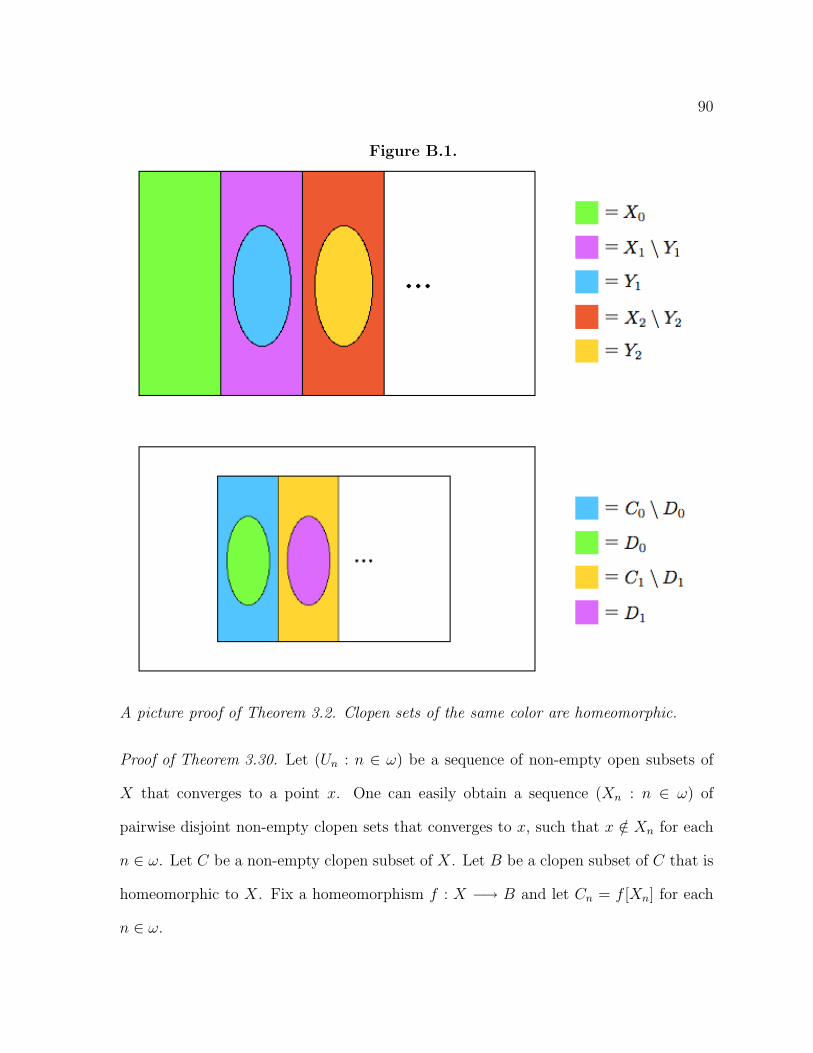
Theorem 3.2 (Terada). Assume that X is non-pseudocompact. If X has a π-base
consisting of clopen sets that are homeomorphic to X then X is h-homogeneous.
The proof of Theorem 3.2 uses the fact that a zero-dimensional non-pseudocompact
space can be written as the disjoint union of infinitely many of its non-empty clopen
subsets (the converse is also true, trivially). However, that is the only consequence of
zero-dimensionality that is actually used (see Appendix B). Therefore such assumption
is redundant by the following lemma.
Lemma 3.3. Assume that X has a π-base B consisting of clopen sets. If X is non-
pseudocompact then X can be written as the disjoint union of infinitely many of its
non-empty clopen subsets.
58
Proof. Let f : X −→ R be an unbounded continuous function. Then the range of f
contains a countably infinite subset D that is closed and discrete as a subset of R. Let
D = {dn : n ∈ ω} be an injective enumeration. Choose pairwise disjoint open sets Un
such that dn ∈ Un for each n ∈ ω. Then choose open sets Vn such that dn ∈ Vn ⊆
cl(Vn) ⊆ Un and diam(Vn) ≤ 2−n for each n ∈ ω.
Next, we will show that V =⋃
n∈ω cl(Vn) is closed. Pick y /∈ V . Choose N ∈ ω big
enough so that 2−N < d(y, D) and let W be the open ball around y of radius 2−(N+1).
We claim that W ∩Vn = ∅ for every n ≥ N + 1. Otherwise, for an element z of such an
which is a contradiction. So W \ (cl(V0) ∪ · · · ∪ cl(VN)) is an open neighborhood of y
that is disjoint from V .
Finally, fix Bn ∈ B such that Bn ⊆ f−1[Vn] for each n ∈ ω. We will show that
B =⋃
n∈ω Bn is clopen, concluding the proof. Pick x /∈ B. If x ∈ f−1[Un] for some n ∈ ω,
then f−1[Un] \ Bn is an open neighborhood of x that is disjoint from B. Now assume
that x /∈⋃
n∈ω f−1[Un]. Then y = f(x) /∈ V , so we can find an open neighborhood W of
y that is disjoint from V . It is clear that f−1[W ] is an open neighborhood of x that is
disjoint from B.
Using Theorem 3.2 one can easily prove the following.
Theorem 3.4 (Terada). Assume that X =∏
i∈I Xi is non-pseudocompact. If Xi is
h-homogeneous and it has a π-base consisting of clopen sets for every i ∈ I then X is
h-homogeneous.
59
In the next section we will introduce the tools that (together with Glickberg’s Theo-
rem 3.20) will ultimately allow us to prove Theorem 3.25, which complements Theorem
3.4. In the process, we will also generalize and exploit some results from Section 2.1, in
order to obtain further partial results on products of h-homogeneous spaces (see Corol-
lary 3.17 and Corollary 3.15).
3.2 Strong CLP-rectangularity
Definition 3.5. A product space X =∏
i∈I Xi is strongly CLP-rectangular if every
clopen subset of X can be written as the union of a collection of pairwise disjoint clopen
rectangles.
The following theorem will be the key to showing that h-homogeneity is preserved
under products in certain cases.
Theorem 3.6. Let Xi be h-homogeneous for every i ∈ I. If C is a non-empty clopen
subset of X =∏
i∈I Xi that can be written as the disjoint union of clopen rectangles then
C ≈ X.
Proof. Let C be a non-empty clopen subset of X such that C =⋃R, where R is a
collection of pairwise disjoint non-empty clopen rectangles. Observe that R ≈ X for
every R ∈ R. In particular the result is trivial if |R| = 1. If |R| > 1 then X is
disconnected, so Xi is disconnected for some i ∈ I. Since Xi is also h-homogeneous,
it follows that Xi ≈ n × Xi whenever 1 ≤ n < ω. Therefore X × n ≈ X whenever
1 ≤ n < ω. So the theorem is established for |R| < ω.
60
Finally, assume that κ = |R| is an infinite cardinal. Then
C ≈ κ×X
≈ (X \ C)⊕ C ⊕ (κ×X)
≈ (X \ C)⊕ (κ×X)
≈ X,
which concludes the proof.
Corollary 3.7. Let Xi be h-homogeneous for every i ∈ I. If X =∏
i∈I Xi is strongly
CLP-rectangular then X is h-homogeneous.
Trivially, every strongly CLP-rectangular product space is CLP-rectangular. The
next theorem shows that, in some cases, the reverse implication holds. However, the
reverse implication does not hold in general (see Proposition 3.18). We will need the
following obvious definition and a cute (even if I say so myself) ‘geometric’ lemma, that
will also be useful in Section 3.3.
Definition 3.8. A space X is CLP-Lindelof if every cover of X consisting of clopen
sets has a countable subcover.
Lemma 3.9. Assume that C is a clopen subset of X×Y that can be written as a boolean
combination of finitely many rectangles. Then C can be written as the union of finitely
many pairwise disjoint clopen rectangles.
Proof. For every x ∈ X, let Cx = {y ∈ Y : (x, y) ∈ C} be the corresponding vertical
cross-section. For every y ∈ Y , let Cy = {x ∈ X : (x, y) ∈ C} be the corresponding
horizontal cross-section. Since C is clopen, each cross-section is clopen.
61
Let A be the Boolean subalgebra of Clop(X) generated by {Cy : y ∈ Y }. Since A is
finitely generated, it is finite (see Corollary 4.5 in [32]). Hence A is isomorphic to the
power set algebra of a finite set (see Corollary 2.8 in [32]). Let P1, . . . , Pm be the atoms
of A. Similarly, let B be the Boolean subalgebra of Clop(Y ) generated by {Cx : x ∈ X},
and let Q1, . . . , Qn be the atoms of B.
Observe that the rectangles Pi × Qj are clopen and pairwise disjoint. Furthermore,
given any i, j, either Pi × Qj ⊆ C or (Pi × Qj) ∩ C = ∅. Hence C is the union of a
(finite) collection of such rectangles.
Corollary 3.10. Assume that C is a clopen subset of∏
i∈I Xi that can be written as a
boolean combination of finitely many rectangles. Then C can be written as the union of
finitely many pairwise disjoint clopen rectangles.
Proof. The case |I| < ω can be established by induction starting from Lemma 3.9. The
case |I| ≥ ω follows, because any boolean combination of finitely many rectangles only
depends on finitely many coordinates.
Theorem 3.11. Assume that X =∏
i∈I Xi is CLP-Lindelof and let C be a clopen subset
of X. If C can be written as the union of clopen rectangles them C can be written as
the union of a countable collection of pairwise disjoint open rectangles.
Proof. Assume that C =⋃Q, where Q is a collection of clopen rectangles. Since X
is CLP-Lindelof, we can assume without loss of generality that Q = {Qn : n ∈ ω} is
countable.
By Corollary 3.10, given any n ∈ ω, it is possible to write
Qn \ (Q0 ∪ · · · ∪Qn−1) =⋃Rn,
62
where Rn is a finite collection of pairwise disjoint clopen rectangles in X. Clearly
R =⋃
n∈ω Rn is the desired countable collection.
Corollary 3.12. If X =∏
i∈I Xi is CLP-Lindelof and CLP-rectangular then X is
strongly CLP-rectangular.
Corollary 3.13. Let Xi be h-homogeneous for every i ∈ I. If X =∏
i∈I Xi is CLP-
Lindelof and CLP-rectangular then X is h-homogeneous.
Corollary 3.14. Let Xi be h-homogeneous for every i ∈ I. If X =∏
i∈I Xi is CLP-
compact then X is h-homogeneous.
Proof. Simply apply Proposition 2.10 and Corollary 3.13.
Corollary 3.15. Let X = X1 × · · · ×Xn. If each Xi is h-homogeneous, CLP-compact
and sequential then X is h-homogeneous.
Proof. Notice that X is CLP-compact by Theorem 2.2.
For example, it follows from Corollary 3.15 that every finite power of the Knaster-
Kuratowski K fan is h-homogeneous (see also Question 4.16).
Combining Kunen’s result from Section 2.1 with the above theorem, we will obtain a
further partial result on products of h-homogeneous spaces. Notice that the following is
an improvement of Corollary 2.12, where we weaken the assumption of σ-compactness
to paracompactness, and we strengthen the conclusion of CLP-rectangularity to strong
CLP-rectangularity.
Corollary 3.16. Let X = X1×· · ·×Xn. If each Xi is locally compact and paracompact
then X is strongly CLP-rectangular.
63
Proof. By the proof of Theorem 5.1.27 in [19], each Xi is the disjoint sum of σ-compact
clopen sets. So X will be the disjoint sum of clopen sets in the form S = S1 × · · · × Sn,
where each Si ⊆ Xi is locally compact and σ-compact. Fix one such product S. Notice
that S is CLP-rectangular by Corollary 2.12. Furthermore, since S is σ-compact, it
is Lindelof, hence CLP-Lindelof. So S is strongly CLP-rectangular by Corollary 3.12,
which concludes the proof.
Corollary 3.17. Let X = X1 × · · · ×Xn. If each Xi is h-homogeneous, locally compact
and paracompact then X is h-homogeneous.
We conclude this section with the promised counterexample. For all the set-theoretic
notions, see [34].
Proposition 3.18 (Kunen). There exists a product space X×Y that is CLP-rectangular
but not strongly CLP-rectangular.
Proof. Let κ be a regular uncountable cardinal with the order topology. Let X and Y
be disjoint stationary subsets of κ. One can easily check that the set
C = {(x, y) ∈ X × Y : x < y} = (X × Y ) ∩ {(x, y) ∈ κ2 : x ≤ y}
consisting of the points above the diagonal is clopen. Since X and Y are both zero-
dimensional, the set C can be written as the union of clopen rectangles.
Assume, in order to get a contradiction, that C =⋃R, where R is a collection of
pairwise disjoint clopen rectangles in X × Y . Whenever (x, y) ∈ C, we will denote by
R(x,y) the unique element of R that contains (x, y). Fix x ∈ X. For every y ∈ Y such
that y > x, choose β(x,y) < y such that {x} × ((β(x,y), y] ∩ Y ) ⊆ R(x,y). By the Pressing
Down Lemma, there must be a stationary subset Tx ⊆ Y of κ and βx ∈ κ such that
64
β(x,y) = βx for every y ∈ Tx. Now let yx be the least element of Tx and let Rx = R(x,yx).
Since the elements of R are pairwise disjoint, it follows that
{x} × ((βx, κ) ∩ Y ) ⊆ Rx
for every x ∈ X.
For every x in X let αx < x be such that ((αx, x]∩X)× ((βx, κ)∩ Y ) ⊆ Rx. By the
Pressing Down Lemma, there must be a stationary subset S ⊆ X of κ and α ∈ κ such
that αx = α for every x ∈ S.
Finally, fix x0 ∈ S and pick x1 ∈ S such that x0 < yx0 ≤ x1 < yx1 . Observe that
(x0, yx1) ∈ Rx0 because βx0 < yx0 ≤ yx1 . On the other hand, (x0, yx1) ∈ Rx1 because
αx1 = αx0 < x0 ≤ x1 and βx1 < yx1 . Therefore Rx0 and Rx1 are the same rectangle
R. Since (x0, yx0) ∈ Rx0 and (x1, yx1) ∈ Rx1 , it follows that (x1, yx0) ∈ R ⊆ C, which
contradicts the definition of C.
3.3 The productivity of h-homogeneity, part II
For a nice introduction to βX, see [50]. Given any open subset U of X, define Ex(U) =
βX \ clβX(X \ U). For proofs of the following facts, see Appendix C.
• Ex(U) is the biggest open subset of βX such that its intersection with X is U .
• If C is a clopen subset of X then Ex(C) = clβX(C), hence Ex(C) is clopen in βX.
• The collection {Ex(U) : U is open in X} is a base for βX.
We remark that it is not true that βX is zero-dimensional whenever X is zero-
dimensional (see Example 6.2.20 in [19] or Example 3.39 in [72]). If βX is zero-
dimensional then X is called strongly zero-dimensional.
65
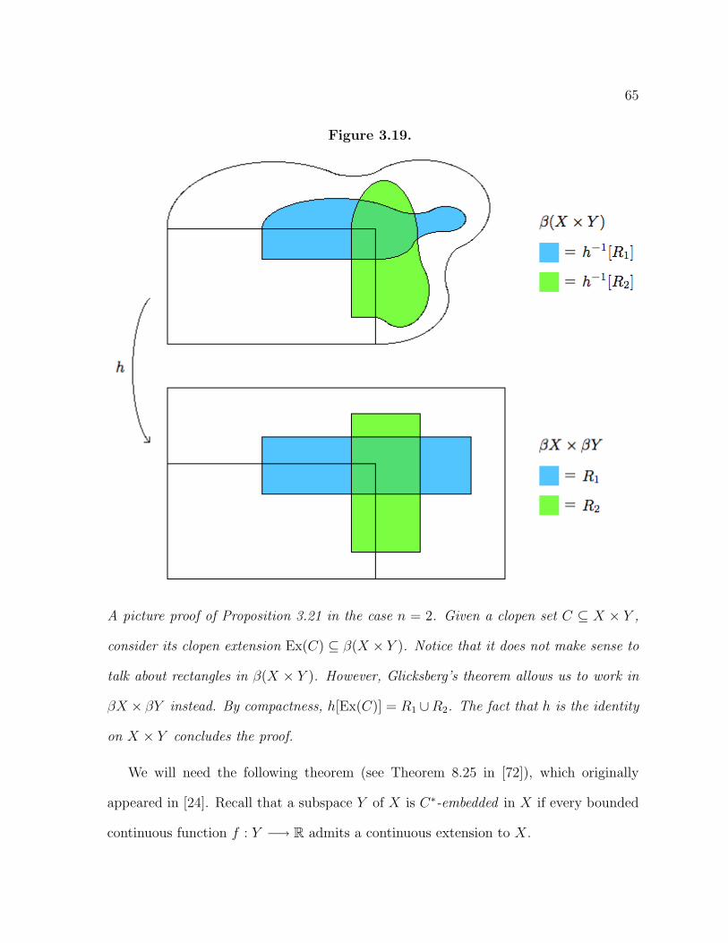
Figure 3.19.
A picture proof of Proposition 3.21 in the case n = 2. Given a clopen set C ⊆ X × Y ,
consider its clopen extension Ex(C) ⊆ β(X × Y ). Notice that it does not make sense to
talk about rectangles in β(X × Y ). However, Glicksberg’s theorem allows us to work in
βX × βY instead. By compactness, h[Ex(C)] = R1 ∪R2. The fact that h is the identity
on X × Y concludes the proof.
We will need the following theorem (see Theorem 8.25 in [72]), which originally
appeared in [24]. Recall that a subspace Y of X is C∗-embedded in X if every bounded
continuous function f : Y −→ R admits a continuous extension to X.
66
Theorem 3.20 (Glicksberg). Assume that X =∏
i∈I Xi is pseudocompact. Then X is
C∗-embedded in∏
i∈I βXi.
The reverse implication is also true, under the additional assumption that∏
j 6=i Xj is
infinite for every i ∈ I. Such assumption is clearly not needed in the above statement
(see Proposition 8.2 in [72]).
Proposition 3.21. Assume that X × Y is pseudocompact. If C is a clopen subset of
X × Y then C can be written as the union of finitely many open rectangles.
Proof. First observe that X×Y is C∗-embedded in βX×βY by Theorem 3.20. Therefore,
by the universal property of the Cech-Stone compactification (see Corollary 3.6.3 in [19]),
there exists a homeomorphism h : β(X × Y ) −→ βX × βY such that h � (X × Y ) is the
identity.
Let C be a clopen subset of X × Y . Notice that h[Ex(C)] will be a clopen sub-
set of βX × βY . Since {Ex(U) : U is open in X} is a base for βX and {Ex(V ) :
V is open in Y } is a base for βY , the collection
B = {Ex(U)× Ex(V ) : U is open in X and V is open in Y }
is a base for βX × βY . Therefore, by compactness, it is possible to write h[Ex(C)] =
R1 ∪ · · · ∪Rn for some n ∈ ω, where Ri = Ex(Ui)× Ex(Vi) ∈ B for each i.
Finally, since h−1 � (X × Y ) is the identity, we get
C = Ex(C) ∩ (X × Y )
= h−1[R1 ∪ · · · ∪Rn] ∩ (X × Y )
= (R1 ∪ · · · ∪Rn) ∩ (X × Y )
67
= (R1 ∩ (X × Y )) ∪ · · · ∪ (Rn ∩ (X × Y ))
= (U1 × V1) ∪ · · · ∪ (Un × Vn),
which concludes the proof.
An obvious modification of the above proof yields the following.
Proposition 3.22. Assume that X =∏
i∈I Xi is pseudocompact. If C is a clopen subset
of X then C can be written as the union of finitely many open rectangles.
Corollary 3.23. Assume that X =∏
i∈I Xi is pseudocompact. If C is a clopen subset
of X then C depends on finitely many coordinates.
We remark that the zero-dimensional case of Corollary 3.23 is a trivial consequence of a
result by Broverman (see Theorem 2.6 in [7]).
Corollary 3.24. Assume that X =∏
i∈I Xi is pseudocompact. Then X is strongly
CLP-rectangular.
Proof. Apply Proposition 3.22 and Corollary 3.10.
Theorem 3.25. Assume that X =∏
i∈I Xi is pseudocompact. If Xi is h-homogeneous
for every i ∈ I then X is h-homogeneous.
Proof. Apply Corollary 3.24 and Corollary 3.7.
Theorem 3.26. If Xi is h-homogeneous and it has a π-base consisting of clopen sets
for every i ∈ I then X =∏
i∈I Xi is h-homogeneous.
Proof. If X is pseudocompact, apply Theorem 3.25; if X is non-pseudocompact, apply
Theorem 3.4.
68
Corollary 3.27. If Xi is h-homogeneous and zero-dimensional for every i ∈ I then∏i∈I Xi is h-homogeneous.
A natural problem that remains open is whether the zero-dimensionality requirement
can be dropped in the above corollary (see Question 4.15).
3.4 Some applications
The compact case of the following result was essentially proved by Motorov (see Theorem
0.2(9) in [52] and Theorem 2 in [51]).
Theorem 3.28. Assume that X has a π-base B consisting of clopen sets. Then Y =
(X × 2×∏B)κ is h-homogeneous for every infinite cardinal κ.
Proof. One can easily check that Y has a π-base consisting of clopen sets that are
homeomorphic to Y . Therefore, if Y is non-pseudocompact, the result follows from
Theorem 3.2.
On the other hand, an analysis of Motorov’s proof shows that the only consequence
of the compactness of Y that is used is the fact that clopen sets in Y depend on finitely
many coordinates. Therefore the same proof works if Y is pseudocompact by Corollary
3.23. We reproduce such proof for the convenience of the reader.
Assume that Y is pseudocompact and let C be a non-empty clopen subset of Y .
The fact that C depends on finitely many coordinates (see Corollary 3.23) implies that
C ≈ Y × C. So it will be enough to show that Y × C ≈ Y .
Let B be a clopen subset of C that is homeomorphic to Y . Let D = C \ B and
E = (Y \C)⊕B. Observe that Y ≈ Y 2 ≈ (Y ×D)⊕(Y ×E) and that Y ⊕Y ≈ 2×Y ≈ Y .
69
Therefore
Y × C ≈ (Y ×D)⊕ (Y ×B)
≈ (Y ×D)⊕ Y 2
≈ (Y ×D)⊕ ((Y ×D)⊕ (Y × E))
≈ ((Y ⊕ Y )×D)⊕ (Y × E)
≈ (Y ×D)⊕ (Y × E)
≈ Y,
which concludes the proof.
Corollary 3.29. For every non-empty zero-dimensional space X there exists a non-
empty zero-dimensional space Y such that X × Y is h-homogeneous. Furthermore, if X
is compact, then Y can be chosen to be compact.
In [70], using a very brief and elegant argument, Uspenskiı proved that for every
non-empty space X there exists a non-empty space Y such that X ×Y is homogeneous.
However, it is not true that Y can be chosen to be compact whenever X is compact:
Motorov proved that the closure in the plane of {(x, sin(1/x)) : x ∈ (0, 1]} is not the
retract of any compact homogeneous space (see Section 3 in [2] for a proof). Corollary
3.29 is an h-homogeneous analog of Uspenskiı’s result. We do not know whether it holds
in the non-zero-dimensional case (see Question 4.18).
The following was proved by Matveev (see Proposition 3 in [37]) under the additional
assumption that X is zero-dimensional, even though such assumption is not actually used
in the proof (see Appendix B). Recall that a sequence (An : n ∈ ω) of subsets of a space
X converges to a point x if for every neighborhood U of x there exists N ∈ ω such that
70
An ⊆ U for each n ≥ N .
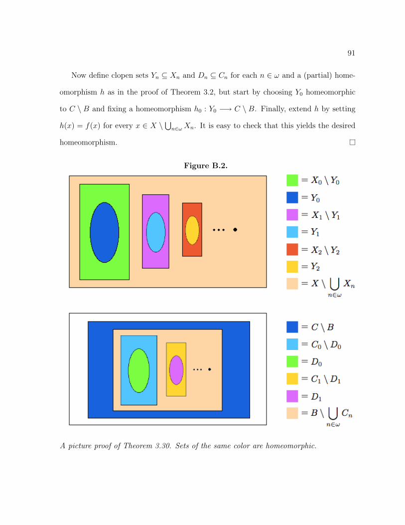
Theorem 3.30 (Matveev). Assume that X has a π-base consisting of clopen sets that
are homeomorphic to X. If there exists a sequence (Un : n ∈ ω) of non-empty open
subsets of X that converges to a point then X is h-homogeneous.
The case κ = ω of the following result is an easy consequence of Theorem 3.30.
Motorov first proved it under the additional assumption that X is a zero-dimensional
first-countable compact space (see Theorem 0.2(2) in [52] and Theorem 1 in [51]). Terada
proved it for an arbitrary infinite κ, under the additional assumption that X is zero-
dimensional and non-pseudocompact (see Corollary 3.2 in [69]).
Theorem 3.31. Assume that X is a space such that the isolated points are dense. Then
Xκ is h-homogeneous for every infinite cardinal κ.
Proof. We will show that Xω is h-homogeneous and it has a π-base consisting of clopen
sets. Since Xκ ≈ (Xω)κ for every infinite cardinal κ, an application of Theorem 3.26
will conclude the proof.
Let D be the set of isolated points of X and let Fn(ω,D) be the set of finite partial
functions from ω to D. Given s ∈ Fn(ω,D), define Us = {f ∈ Xω : f ⊇ s}. Now fix
d ∈ D and let g ∈ Xω be the constant function with value d. It is easy to see that
(Ug�n : n ∈ ω) is a sequence of open sets in Xω that converges to g. Furthermore B =
{Us : s ∈ Fn(ω,D)} is a π-base for Xω consisting of clopen sets that are homeomorphic
to Xω. So Xω is h-homogeneous by Theorem 3.30.
71
3.5 Infinite powers of zero-dimensional first-countable
spaces
The following proposition is folklore, and it explains why h-homogeneous spaces are
sometimes called ‘strongly homogeneous’. Recall that a space X is homogeneous if for
every x, y ∈ X there exists a homeomorphism h : X −→ X such that h(x) = y.
Proposition 3.32. Assume that X is a zero-dimensional first-countable space. If X is
h-homogeneous then X is homogeneous.
Proof. Assume that X is h-homogeneous. Fix x, y ∈ X. Choose local bases {Un : n ∈ ω}
and {Vn : n ∈ ω} at x and y respectively so that the following conditions are satisfied.
• All Un and Vn are clopen.
• U0 ∩ V0 = ∅.
• Un+1 ( Un and Vn+1 ( Vn for every n ∈ ω.
By h-homogeneity, for every n ∈ ω, there exists a homeomorphism
hn : Un \ Un+1 −→ Vn \ Vn+1.
It is easy to see that⋃
n∈ω(hn∪h−1n ) can be extended to a homeomorphism h : X −→ X
such that h(x) = y and h(y) = x.
72
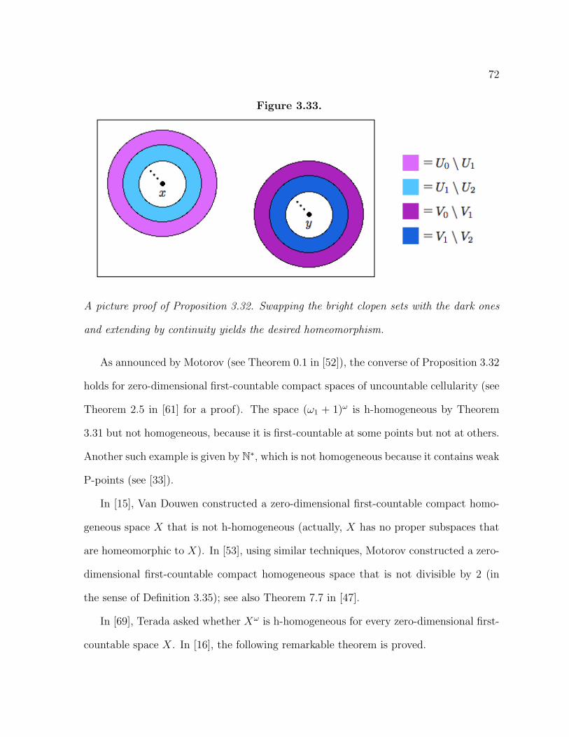
Figure 3.33.
A picture proof of Proposition 3.32. Swapping the bright clopen sets with the dark ones
and extending by continuity yields the desired homeomorphism.
As announced by Motorov (see Theorem 0.1 in [52]), the converse of Proposition 3.32
holds for zero-dimensional first-countable compact spaces of uncountable cellularity (see
Theorem 2.5 in [61] for a proof). The space (ω1 + 1)ω is h-homogeneous by Theorem
3.31 but not homogeneous, because it is first-countable at some points but not at others.
Another such example is given by N∗, which is not homogeneous because it contains weak
P-points (see [33]).
In [15], Van Douwen constructed a zero-dimensional first-countable compact homo-
geneous space X that is not h-homogeneous (actually, X has no proper subspaces that
are homeomorphic to X). In [53], using similar techniques, Motorov constructed a zero-
dimensional first-countable compact homogeneous space that is not divisible by 2 (in
the sense of Definition 3.35); see also Theorem 7.7 in [47].
In [69], Terada asked whether Xω is h-homogeneous for every zero-dimensional first-
countable space X. In [16], the following remarkable theorem is proved.
73
Theorem 3.34 (Dow and Pearl). If X is a zero-dimensional first-countable space then
Xω is homogeneous.
However, Terada’s question remains open, even for separable metric spaces (but see
Corollary 3.43 and the remarks before Proposition 3.42). In [51] and [52], Motorov asks
whether such an infinite power is always divisible by 2. Using Theorem 3.34, we will
show that the two questions are equivalent: actually even weaker conditions suffice (see
Proposition 3.38).
Definition 3.35. A space F is a factor of X (or X is divisible by F ) if there exists Y
such that F × Y ≈ X. If F ×X ≈ X then F is a strong factor of X (or X is strongly
divisible by F ).
We will use the following lemma freely in the rest of this section.
Lemma 3.36. The following are equivalent.
1. F is a factor of Xω.
2. F is a strong factor of Xω.
3. F ω is a strong factor of Xω.
Proof. The implications (2) → (1) and (3) → (1) are clear.
Assume that (1) holds. Then there exists Y such that F × Y ≈ Xω, hence
Xω ≈ (Xω)ω ≈ (F × Y )ω ≈ F ω × Y ω.
Since multiplication by F or by F ω does not change the right-hand side, it follows that
(2) and (3) hold.
74
Lemma 3.37. Assume that Y is a non-empty zero-dimensional first-countable space.
Then X = (Y ⊕ 1)ω is h-homogeneous and X ≈ Y ω × (Y ⊕ 1)ω ≈ 2ω × Y ω.
Proof. Recall that 1 = {0} and let g ∈ X be the constant function with value 0. For
each n ∈ ω, define
Un = {f ∈ X : f(i) = 0 for all i < n}.
Observe that B = {Un : n ∈ ω} is a local base for X at g consisting of clopen sets
that are homeomorphic to X. But X is homogeneous by Theorem 3.34, therefore it has
such a local base at every point. In conclusion X has a base (hence a π-base) consisting
of clopen sets that are homeomorphic to X. It follows from Theorem 3.30 that X is
h-homogeneous.
To prove the second statement, observe that
X ≈ (Y ⊕ 1)×X ≈ (Y ×X)⊕X,
hence X ≈ Y ×X by h-homogeneity. It follows that X ≈ Y ω × (Y ⊕ 1)ω. Finally,
Y ω × (Y ⊕ 1)ω ≈ (Y ω × (Y ⊕ 1))ω ≈ (Y ω ⊕ Y ω)ω ≈ 2ω × Y ω,
that concludes the proof.
Proposition 3.38. Assume that X is a zero-dimensional first-countable space contain-
ing at least two points. Then the following are equivalent.
1. Xω ≈ (X ⊕ 1)ω.
2. Xω ≈ Y ω for some space Y with at least one isolated point.
3. Xω is h-homogeneous.
75
4. Xω has a non-empty clopen subset that is strongly divisible by 2.
5. Xω has a proper clopen subset that is homeomorphic to Xω.
6. Xω has a proper clopen subset that is a factor of Xω.
Proof. The implication (1) → (2) is trivial; the implication (2) → (3) follows from
Lemma 3.37; the implications (3) → (4) → (5) → (6) are trivial.
Assume that (6) holds. Let C be a proper clopen subset of Xω that is a factor of
Xω and let D = Xω \ C. Then
Xω ≈ (C ⊕D)×Xω
≈ (C ×Xω)⊕ (D ×Xω)
≈ Xω ⊕ (D ×Xω)
≈ (1⊕D)×Xω,
hence Xω ≈ (1⊕D)ω ×Xω. Since (1⊕D)ω ≈ 2ω ×Dω by Lemma 3.37, it follows that
2ω is a factor of Xω. So 2ω is a strong factor of Xω. Therefore (1) holds by Lemma
3.37.
The next two propositions show that in the pseudocompact case we can say something
more.
Proposition 3.39. Assume that X is a zero-dimensional first-countable space such that
Xω is pseudocompact. Then Cω ≈ (X ⊕ 1)ω for every non-empty proper clopen subset
C of Xω.
Proof. Let C be a non-empty proper clopen subset of Xω. It follows from Corollary
3.23 that C ≈ C × Xω, hence Cω ≈ Cω × Xω. Since Cω × Xω clearly has a proper
76
clopen subset that is homeomorphic to Cω × Xω, Proposition 3.38 implies that Cω is
h-homogeneous, hence strongly divisible by 2. So Cω ≈ 2ω ×Cω ≈ 2ω ×Cω ×Xω. Since
2ω ×Xω ≈ (X ⊕ 1)ω by Lemma 3.37, it follows that Cω ≈ Cω × (X ⊕ 1)ω.
On the other hand, (X ⊕ 1)ω ≈ Xω × (X ⊕ 1)ω by Lemma 3.37. Hence (X ⊕ 1)ω has
a clopen subset homeomorphic to C × (X ⊕ 1)ω. But Lemma 3.37 shows that (X ⊕ 1)ω
is h-homogeneous, so C × (X ⊕ 1)ω ≈ (X ⊕ 1)ω. Therefore Cω × (X ⊕ 1)ω ≈ (X ⊕ 1)ω,
that concludes the proof.
Proposition 3.40. In addition to the hypotheses of Proposition 3.38, assume that Xω
is pseudocompact. Then the following can be added to the list of equivalent conditions.
(7) Xω has a non-empty proper clopen subset that is homeomorphic to Y ω for some
space Y .
Proof. The implication (5) → (7) is trivial.
Assume that (7) holds. Let C be a non-empty proper clopen subset of Xω that is
homeomorphic to Y ω for some space Y . Then clearly Cω ≈ C. Therefore C ≈ (X ⊕ 1)ω
by Proposition 3.39. Hence C is strongly divisible by 2 by Lemma 3.37, showing that
(4) holds.
Finally, we point out that Proposition 3.38 can be used to give a positive answer to
Terada’s question for a certain class of spaces. We will need the following definition.
Definition 3.41. A space X is ultraparacompact if every open cover of X has a re-
finement consisting of pairwise disjoint clopen sets.
It is easy to see that every ultraparacompact space is zero-dimensional. As noted
by Nyikos in [54], a space is ultraparacompact if and only if it is paracompact and
77
strongly zero-dimensional (this is proved like Proposition 1.2 in [17]). A metric space
X is ultraparacompact if and only if dim X = 0 (see Theorem 7.2.4 in [19]); see also
Theorem 7.3.3 in [19]. For such a metric space X, Van Engelen proved that Xω is h-
homogeneous if X is meager in itself or X has a completely metrizable dense subset (see
Theorem 4.2 and Theorem 4.4 in [18]). It follows that Xω is h-homogeneous if X is a
subset with the property of Baire in the restricted sense of some completely metrizable
space (see Corollary D.2). In particular, this holds if X is in the σ-algebra generated by
the analytic subsets of some completely metrizable space (see Corollary D.4). Similar
result were obtained independently by Ostrovskiı (see Theorem 8 and Theorem 9 in [56]).
See also the discussion that follows Corollary 3.43. However, according to Medvedev,
the proof of Theorem 4.3 in [18] contains a gap (which he fixed: see Remark 4 in [43]).
Proposition 3.42. Assume that X is a (zero-dimensional) first-countable space. If Xω
is ultraparacompact and non-Lindelof then Xω is h-homogeneous.
Proof. Let U be an open cover of Xω with no countable subcovers. By ultraparacom-
pactness, there exists a refinement V of U consisting of pairwise disjoint non-empty
clopen sets. Let V = {Cα : α ∈ κ} be an enumeration without repetitions, where κ is
an uncountable cardinal.
Now fix x ∈ Xω and a local base {Un : n ∈ ω} at x consisting of clopen sets. Since
Xω is homogeneous by Theorem 3.34, for each α < κ we can find n(α) ∈ ω such that
a homeomorphic clopen copy Dα of Un(α) is contained in Cα. Since κ is uncountable,
there exists an infinite S ⊆ κ such that n(α) = n(β) for every α, β ∈ S. It is easy to
check that⋃
α∈S Dα is a non-empty clopen subset of Xω that is strongly divisible by 2.
Therefore Xω is h-homogeneous by Proposition 3.38.
78
An application of Corollary 4.1.16, Theorem 7.3.2 and Theorem 7.3.16 in [19] imme-
diately yields the following result.
Corollary 3.43. Assume that X is a metric space such that dim X = 0. If X is non-
separable then Xω is h-homogeneous.
We conclude this chapter with two remarks about Theorem 25 in [43], which was
obtained independently by Medvedev and overlaps with the above corollary. The first
remark is that the statement of such theorem contains an inaccuracy: to make the
proof work, X should be required to have the property of Baire in the restricted sense
(see Appendix D), not just the property of Baire. In fact, the property of Baire is not
enough to obtain the dichotomy given by Proposition D.1 (see the remark preceding it).
The second remark is that by Corollary 3.43, in the non-separable case, no additional
requirement on X is needed anyway.
79
Chapter 4
Open problems
4.1 The topology of ultrafilters as subspaces of the
Cantor set
In this section, we will follow the same conventions of Chapter 1. Since most of our main
constructions need some additional set-theoretic assumption (namely, Martin’s Axiom
for countable posets), in each case it is natural to ask whether such assumption can be
dropped. Questions 4.1, 4.2 and 4.3 first appeared as Questions 2, 3 and 7 respectively
in [41]. As we explained in Section 1.8, it follows from a result of Shelah that it is not
possible to construct in ZFC an ultrafilter U ⊆ 2ω that is completely Baire.
Question 4.1. Is it possible to construct in ZFC an ultrafilter U ⊆ 2ω that is not
countable dense homogeneous?1
Question 4.2. Is it possible to construct in ZFC an ultrafilter U ⊆ 2ω that is countable
dense homogeneous?
Question 4.3. Is it possible to construct in ZFC an ultrafilter U ⊆ 2ω such that A ∩ U
has the perfect set property whenever A is an analytic subset of 2ω?
1Very recently, Repovs, Zdomskyy and Zhang constructed in ZFC a non-meager filter F ⊆ 2ω thatis not countable dense homogeneous (see [59]).
80
The case of countable dense homogeneity seems particularly interesting because at this
point it is still conceivable that there exists a model of ZFC in which every ultrafilter is
countable dense homogeneous and one in which no ultrafilter is countable dense homo-
geneous. Certainly, by Theorem 1.15 and Theorem 1.21, there exists a model of ZFC in
which both kinds of ultrafilter exist (take any model of MA(countable)).
Regarding the relation between P-points and the topological properties that we in-
vestigated, we remark that the following four questions remain open (see the discussion
in Section 1.8). Questions 4.4, 4.6 and 4.7 first appeared as Question 11, the first half
of Question 12 and the second half of Question 12 respectively in [41].
Question 4.4. Is it possible to prove in ZFC that every P-point U ⊆ 2ω is countable
dense homogeneous?2
Question 4.5. Is it possible to prove in ZFC that every countable dense homogeneous
ultrafilter U ⊆ 2ω is a P-point?
Question 4.6. Is it possible to prove in ZFC that if U ⊆ 2ω is a P-point then A ∩ U
has the perfect set property whenever A is an analytic subset of 2ω?
Question 4.7. Is it possible to prove in ZFC that if U ⊆ 2ω is an ultrafilter such that
A ∩ U has the perfect set property whenever A is an analytic subset of 2ω then U is a
P-point?
Observe that Lemma 1.33 might be viewed as a partial answer to Question 4.6.
We conclude this section by mentioning two isolated questions that remain open.
The first one aims at ‘optimizing the definability’ of X in Question 1.23, and it first
appeared as Question 6 in [41].
2While this thesis was being written, Hernandez-Gutierrez and Hrusak showed that F and Fω areboth countable dense homogeneous whenever F ⊆ 2ω is a non-meager P-filter (see [25]).
81
Question 4.8. Is it consistent that there exists an analytic non-Gδ subset X of 2ω such
that Xω is countable dense homogeneous? Co-analytic?
We are only asking for a consistency result because under Projective Determinacy every
projective countable dense homogeneous space is completely metrizable (see Corollary
2.7 in [26]).
The second one is about the exact consistency strength of an ultrafilter like the one
given by Theorem 1.36, and it first appeared as part of Question 9 in [41].
Question 4.9. Does the Levy collapse Col(ω, κ) of an inaccessible cardinal κ to ω1 force
the existence an ultrafilter U ⊆ 2ω such that A∩U has the perfect set property for every
A ∈ P(2ω) ∩ L(R)?
Notice that Theorem 1.36 implies that such consistency strength is between that of an
inaccessible cardinal and a Mahlo cardinal. If the answer to the above question were
‘yes’, then it would be exactly that of an inaccessible cardinal.
4.2 Products and CLP-compactness
As we mentioned in the introduction to Chapter 2, very little is known about infinite
products when it comes to CLP-compactness. Even the following question (which is
Question 6.4 in [68]), arguably the ‘easiest possible’, is still open.
Question 4.10 (Steprans and Sostak). Let X =∏
i∈ω Xi. If each Xi is CLP-compact
and second-countable, must X be CLP-compact?
To look at a concrete example: Theorem 2.2 implies that every finite power Kn of the
82
Knaster-Kuratowski fan is CLP-compact (hence CLP-rectangular by Proposition 2.10),
but the following question remains open.
Question 4.11. For which infinite cardinals κ is Kκ CLP-compact (equivalently, CLP-
rectangular)?
As observed by Glicksberg in [24] (see also Proposition 8.26 in [72]), a product space
is pseudocompact if and only if every countable subproduct is pseudocompact. Does the
analogous theorem hold for CLP-compactness?
Question 4.12. Let κ be an uncountable cardinal. If {Xξ : ξ ∈ κ} is a collection of
spaces such that∏
ξ∈I Xξ is CLP-compact for every I ∈ [κ]<ω1 does it follow that∏
ξ∈κ Xξ
is CLP-compact? Does this depend on the size of κ?
Notice that the above might be viewed as the natural ‘sequel’ to Question 2.5.
Finally, it is natural to investigate whether the separation properties of our coun-
terexample can be improved.
Question 4.13. In Corollary 2.22, can ‘Hausdorff’ be substituted by ‘regular’?
We will conclude this section by showing that our example is indeed not regular.
Since for zero-dimensional spaces CLP-compactness is equivalent to compactness, it will
be enough to prove that every locally countable regular space is zero-dimensional. This
follows from the fact that countable regular spaces are zero-dimensional (see Corollary
6.2.8 in [19]) and the next proposition.
Proposition 4.14. Assume that X is locally zero-dimensional and regular. Then X is
zero-dimensional.
83
Proof. Fix x ∈ X. We will show that the clopen neighborhoods of x form a local base
of X at x. Let U be an open zero-dimensional neighborhood of x. By regularity, there
exists an open subset V of X such that x ∈ V ⊆ clX(V ) ⊆ U . By zero-dimensionality,
there exists a clopen subset C of U such that x ∈ C ⊆ V .
We claim that C is clopen in X. The fact that C is open in X is obvious. To see
that C is closed in X, notice that clX(C) ⊆ clX(V ) ⊆ U , and therefore C = clU(C) =
clX(C) ∩ U = clX(C).
4.3 Products and h-homogeneity
In this section we implicitly assume that all spaces are Tychonoff. All the work done
in Chapter 3 notwithstanding, it is still an open problem (even in the case of finite
products) whether h-homogeneity is productive. Terada originally posed the problem in
[69], but he was including zero-dimensionality in the definition of h-homogeneity. The
question in its full generality first appeared in [40].
Question 4.15. If Xi is h-homogeneous for every i ∈ I, does it follow that X =∏
i∈I Xi
is h-homogeneous?
Observe that any counterexample X must be non-pseudocompact (by Theorem 3.25)
and non-zero-dimensional (actually, by Theorem 3.26, it cannot even have a π-base
consisting of clopen sets). Also keep in mind that Theorem 3.6, Corollary 3.15 and
Corollary 3.17 hold.
Once again, the Knaster-Kuratowski fan K might be an interesting test space. Recall
that Kn is h-homogeneous for every n ∈ ω by Corollary 3.15. However, we do not know
the answer to the following question.
84
Question 4.16. For which infinite cardinals κ is Kκ h-homogeneous?
Recall that E = {x ∈ `2 : xn ∈ Q for all n ∈ ω} is the Erdos space. It is easy to
see that En ≈ E for every n ∈ ω. It is also true, but hard to prove, that Eω ≈ E (see
Corollary 9.4 in [13]). Therefore Eκ is h-homogeneous whenever κ ≤ ω by Corollary 8.15
in [13]. However, the following question remains open.
Question 4.17. For which uncountable cardinals κ is Eκ h-homogeneous?
Another result which we would like to generalize to the non-zero-dimensional case is
Corollary 3.29. The following question first appeared in [40].
Question 4.18. Is it true that for every non-empty space X there exists a non-empty
space Y such that X × Y is h-homogeneous? If X is compact, can Y be chosen to be
compact?
Together with Question 4.15, we believe the following to be the most interesting open
problem on the topic of h-homogeneity, and Section 3.5 is best viewed as a collection of
partial results towards its solution.
Question 4.19 (Terada). Is Xω h-homogeneous whenever X is a zero-dimensional first-
countable space?
If one drops the ‘h’, then the answer is ‘yes’ by Theorem 3.34, which was proved by Dow
and Pearl in [16]. Since h-homogeneity implies homogeneity for zero-dimensional first-
countable spaces (see Proposition 3.32), a positive answer would give a strenghtening of
their result. Proposition 3.38 suggests a strategy for answering ‘yes’ to Question 4.19:
one could try to use the techniques of [16] to show that condition (1) actually holds for
85
every zero-dimensional first-countable space X. Also observe that the following question
of Motorov (see [51] and [52]) is equivalent to Question 4.19 by Proposition 3.38.
Question 4.20 (Motorov). Is Xω divisible by 2 whenever X is a zero-dimensional first-
countable space containing at least two points?
In the same articles, Motorov asked whether the 2 can be dropped from the definition
of Y in his version of Theorem 3.28. Inspecting our proof reveals that this is possible if
Y is non-pseudocompact, but we do not know the answer in general.
Question 4.21. Assume that X has a π-base B consisting of clopen sets. Does it follow
that Y = (X ×∏B)κ is h-homogeneous for every infinite cardinal κ?
Observe that if the answer were ‘yes’ then Theorem 3.31 would become an immediate
corollary of Theorem 3.28.
86
Appendix A
The Knaster-Kuratowski fan
In this section, we will discuss a space introduced by Knaster and Kuratowski in [31],
which turns out to be an interesting example of h-homogeneous CLP-compact space (see
Proposition A.2). This example is also known as Cantor’s teepee (see Example 129 in
[65]). The exposition is based on Exercise 6.3.23 in [19].
We will work in the plane R2. Identify 2ω with the usual Cantor set in [0, 1] × {0}.
Fix a countable dense subset Q of 2ω, and let P = 2ω \ Q. Let q = (1/2, 1/2). Given
c ∈ 2ω, denote by Lc the half-open line segment connecting c and q, including c but
excluding q. Given c ∈ 2ω, define
Kc =
{(x, y) ∈ Lc : y ∈ Q} if c ∈ Q,
{(x, y) ∈ Lc : y ∈ R \Q} if c ∈ 2ω \Q.
Define K =⋃
c∈2ω Kc and F = K ∪ {q}. We will refer to K as the Knaster-Kuratowski
fan, even though Engelking uses that name for F , because K is much more interesting
than F for our purposes (see Proposition A.3).
Lemma A.1. Assume that C is a clopen subset of K. Then there exists a clopen set C
in 2ω such that C =⋃
c∈ eC Kc.
Proof. Let A = A0 and B = A1 be closed subsets of R2 such that A ∩ K = C and
B ∩K = K \C. Let Q∩ [0, 1/2) = {qn : n ∈ ω} and let Hn = {(x, qn) : x ∈ R} for every