Business School The University of Sydney

OME WORKING PAPER SERIES

The Two-sided Weibull Distribution and Forecasting

Financial Tail Risk

Richard Gerlach Business School

The University of Sydney

Qian Chen Business School

The University of Sydney

Abstract

A two-sided Weibull is developed to model the conditional financial return distribution, for the purpose of forecasting Value at Risk (VaR) and conditional VaR. A range of conditional return distributions are combined with four volatility specifications to forecast tail risk in four international markets, two exchange rates and one individual asset series, over a four year forecast period that includes the recent global financial crisis. The two-sided Weibull performs at least as well as other distributions for VaR forecasting, but performs most favourably for conditional Value at Risk forecasting, prior to as well as during and after the recent crisis.

February 2011

OME Working Paper No: 01/2011 http://www.econ.usyd.edu.au/ome/research/working_papers

The Two-sided Weibull Distribution and Forecasting

Financial Tail Risk

Qian Chena ∗, Richard H. Gerlachb

aDiscipline of Operations Management and Econometrics, University of Sydney, NSW 2006, Australia.

Email: qian.chen@sydney.edu.au.

bDiscipline of Operations Management and Econometrics, University of Sydney, NSW 2006, Australia.

Tel: 612 9351 3944. Fax: 612 9351 6409. Email: richard.gerlach@sydney.edu.au.

∗Corresponding author is Qian Chen. Email: qian.chen@sydney.edu.au.

1

Abstract

A two-sided Weibull is developed to model the conditional financial return dis-

tribution, for the purpose of forecasting Value at Risk (VaR) and conditional VaR.

A range of conditional return distributions are combined with four volatility speci-

fications to forecast tail risk in four international markets, two exchange rates and

one individual asset series, over a four year forecast period that includes the recent

global financial crisis. The two-sided Weibull performs at least as well as other dis-

tributions for VaR forecasting, but performs most favourably for conditional Value

at Risk forecasting, prior to as well as during and after the recent crisis.

Keywords: Two-sided Weibull, Value-at-Risk, Expected shortfall, Back-testing, global

financial crisis, volatility.

1 Introduction

The Global Financial Crisis (GFC) has highlighted that international financial markets

can be subject to very fast changing volatility and risk levels and once again called into

question risk measurement and risk management practices in general. As Basel III starts

its life in 2011, fundamental questions are still being raised and examined concerning

how to measure risk and how, or even if, its level can be forecast accurately. In the

academic literature, much interest has focused on conditional asset return distributions,

which could help solve the second issue if well specified, and in particular on two aspects:

(i) the time-varying nature of the distribution, e.g. volatility; and (ii) the shape and form

of the standardised conditional distribution itself, e.g. Gaussian.

Volatility modelling now has a fairly long history, its importance well-known at least

since the development of the parametric ARCH model in Engle (1982) and subsequently

GARCH in Bollerslev (1986). These 1st generation models were extended to capture

various aspects of observed returns, e.g.: the Exponential-GARCH model of Nelson (1991)

and the GJR-GARCH (GJR) model of Glosten, Jagannathan and Runkle (1993), which

capture the asymmetric volatility effect of Black (1976). More recently, fully nonlinear

GARCH models have been specified, including the threshold (T)-GARCH of Zakoian

(1994), the double threshold (DT)-ARCH of Li and Li (1996); the DT-GARCH of Brooks

(2001) and the smooth transition (ST-)GARCH of Gonzalez-Rivera (1998) and Gerlach

and Chen (2008). Many other models have been proposed that are far too numerous to

mention. We focus on four of these specifications: GARCH, GJR-GARCH, T-GARCH

and ST-GARCH.

Regarding the distribution of returns, there is considerable empirical evidence that

daily asset returns are fat-tailed or leptokurtic, and also mildly negatively skewed (see

e.g. Poon and Granger, 2003, among many others), both unconditionally and condition-

ally. Mandelbrot (1963) and Fama (1965) pioneered the use of non-Gaussian distributions

in finance investigating the stable Paretian and power laws, while Mittnik and Ratchev

(1989) also considered the Weibull, log-normal (separately for positive and negative re-

turns) and Laplace, as unconditional return distributions. Fama (1965) and Barnea and

1

Downes (1973) also considered mixtures of Gaussians in this context. Subsequent to the

1st generation ARCH and GARCH models, and since the extra kurtosis allowed by Gaus-

sian errors does not often fully capture fat-tails in returns, Bollerslev (1987) proposed

the GARCH with conditional Student-t error model; McCulloch (1985) used a simplified

ARCH-type structure with a conditional stable distribution, updated to GARCH by Liu

and Brorsen (1995); Nelson (1982) employed the generalised exponential as a conditional

distribution in his E-GARCH; Vlaar and Palm (1993) used a mixture of Gaussians as

the errors in a GARCH model; while Hansen (1994) developed a skewed Student-t dis-

tribution, combining it with a GARCH model, also allowing both conditional skewness

and kurtosis to change over time. More recently, Zhu and Galbraith (2009) extended

the skewed-t idea by using a generalized asymmetric Student-t conditional distribution,

with separate parameters in each tail; Griffin and Steel (2006) and Jensen and Maheu

(2010) employed Dirichlet process mixtures, while Aas and Haff (2006) used a generalised

hyperbolic, for the conditional return distribution.

Chen, Gerlach and Lu (2011) employed an asymmetric Laplace distribution, devel-

oped by Hinkley and Revankar (1977), combining with a GJR-GARCH model and found

it was the only conditional return distribution considered (they also tried Student-t and

Gaussian) that consistently over-estimated risk levels, and thus was a conservative risk

model, during the GFC period. This paper aims to more accurately estimate risk levels

by employing a natural and more flexible extension of the Laplace: the Weibull, and sub-

sequently developing a two-sided Weibull distribution. After developing this distribution

and its properties, the authors found that Sornette et al (2000) had developed a symmet-

ric, two-sided ’modified’ Weibull, subsequently used in Maleverge and Sornette (2004) as

an unconditional distribution for asset returns, combined with a Gaussian copula, in order

to form efficient portfolios; an asymmetric ’modified’ Weibull was also briefly discussed.

We propose a slightly more flexible asymmetric two-sided Weibull to use as a conditional

return distribution in this paper.

Two of the most well-known and popular modern risk measures are Value-at-Risk

(VaR), pioneered by JP Morgan in 1993, and conditional VaR, or expected shortfall (ES),

proposed by Artzner, Delbaen, Eber and Heath (1997, 1999). VaR represents the market

2

risk as one number: the minimum loss expected on an investment, over a given time

period at a specific quantile level. It is an important regulatory tool, recommended by

the Basel Committee on Banking Supervision in Basel II, to control the risk of finan-

cial institutions, by helping to set minimum capital requirements to protect against large

unexpected losses. However VaR was criticised at least by 1999, when the Bank of Inter-

national Settlements (BIS) Committee pointed out that extreme market movement events

“were in the ’tail’ of distributions, and that VaR models were useless for measuring and

monitoring market risk”. While perhaps an exaggerated comment, VaR clearly does not

measure the magnitude of the loss for violating returns; ES, however, does give the ex-

pected loss (magnitude) conditional on exceeding a VaR threshold. Further, Artzner et al.

(1999) found that VaR is not a ’coherent’ measure: i.e. it is not sub-additive, while ES,

which they proposed, is coherent. Consequently, the use of VaR can (sometimes) lead to

portfolio concentration rather than diversification, while ES cannot. Finally, while VaR

is recommended in Basel II, ES is not. Both are considered here.

Basel II recomends a back-testing procedure for evaluating and comparing VaR mod-

els based on the number of observed violations, i.e. when actual losses exceed the VaR, in

a hold-out sample period of at least one year. Under-estimation of VaR (and ES) levels

can result in setting aside insufficient regularity capital and thus suffering fatal losses

during extreme market movements. Ewerhart (2002) argued that prudent financial insti-

tutions tend to hold unnecessary, excessive regulatory capital to ensure their reputation

and quality, while Bakshi and Panayotov (2007) called this the ‘Capital Charge Puzzle’.

Intuitively, overstated VaR will lead financial institutions to allocate excessive amounts

of capital, which may be attractive in the post-GFC market. However, as the goals of

financial institutions are to meet the regulatory and capital requirements and to maxi-

mize profits and attract investors, such capital over-allocation represents an investment

opportunity cost. Thus, although the regulators may prefer smaller violation numbers

in case of excessive losses, investors favour models adequately predicting risk instead of

over-(or under-) predicting it. The goal of our paper is to find a model achieving that

both prior to as well as during and after the recent GFC.

Parameter estimation and inference is executed via a Bayesian approach with an

3

adaptive Markov chain Monte Carlo (MCMC), adapted from Chen et al (2011). The

rest of the paper is structured as follows: Section 2 introduces the two-sided Weibull

distribution; Section 3 specifies the volatility models considered; Section 4 briefly describes

the Bayesian approach and MCMC methods; Section 5 presents the empirical studies from

four international stock markets, two exchange rates and one individual asset return series,

back-testing a range of models for VaR and ES; Section 6 summarizes.

2 A two-sided Weibull distribution

The Weibull distribution, introduced by Weibull (1951), is a special case of an extreme

value distribution and of the generalised gamma distribution. It is widely applied in the

fields of material science, engineering and also in finance, due to its versatility. Mittnik and

Ratchev (1989) found it to be the most accurate for the unconditional return distribution

for the S&P500 index when applied separately to positive and negative returns; while

various authors have employed it as an error distribution in range data modelling (see

Chen et al, 2008) and trading duration (ACD) models (see e.g. Engle and Russell, 1998).

Sornette et al. (2000) proposed and used a symmetric modified (two-sided) Weibull

distribution as an unconditional return distribution, combined with a Gaussian copula,

to choose efficient portfolios in Malevergne and Sornette (2004); they also mentioned a

two-sided Weibull but did not explore its properties. We introduce a similar, though

more flexible, transformed Weibull, called the two-sided Weibull distribution (TW). The

motivation for this is to capture empirical traits in conditional return distributions such

as fat-tails and skewness for the purposes of risk measure forecasting: thus, the tails are

the most important regions to model accurately. The idea, as in Mittnik and Ratchev

(1989) and Malevergne and Sornette (2004), is to allow a different Weibull distribution

for positive and negative returns. This also sets up a flexible extension of the asymmetric

Laplace (AL) distribution in Chen et al (2011), where a different exponential was allowed

for positive and negative returns; i.e. if X ∼ Exp’l(λ) then Xk ∼Weibull(λ, k).

Since a conditional error in a GARCH-type model needs to have mean 0 and vari-

ance 1, we further develop the standardised two-sided Weibull distribtion (STW). We

4

subsequently derive the pdf, cdf, quantile function and the conditional expectation func-

tions required to calculate the likelihood as well as VaR and ES measures for the STW

distribution.

The TW’s shape and scale can be tuned by four Weibull parameters. The definition

of a TW is, Y ∼ TW (λ1, k1, λ2, k2) if: −Y ∼Weibull(λ1, k1) ; Y < 0

Y ∼Weibull(λ2, k2) ; Y ≥ 0

where the shape parameters satisfy k1, k2 > 0 and scale parameters λ1, λ2 > 0.

2.1 Standardised Two-sided Weibull distribution

Error distributions in volatility models should be standardised. A standardised TW dis-

tribution is equivalent to Y√Var(Y )

. For a TW, it can be shown that:

Var(Y ) = b2p =λ31k1

Γ(

1 +2

k1

)+λ32k2

Γ(

1 +2

k2

)−[−λ

21

k1Γ(

1 +1

k1

)+λ22k2

Γ(

1 +1

k2

)]2.

The pdf for an STW random variable X = Y√Var(Y )

, where Y ∼ TW (λ1, k1, λ2, k2), is:

f(x|λ1, k1, k2) =

bp(−bpxλ1

)k1−1exp

[−(−bpxλ1

)k1]; x < 0

bp(bpxλ2

)k2−1exp

[−(bpxλ2

)k2]; x ≥ 0

(1)

To ensure the pdf integrates to 1:

λ1k1

+λ2k2

= 1 (2)

Thus, in this formulation there are only three free parameters, and we write X ∼

STW (λ1, k1, k2) where λ2 is fixed by (2). In this parametrization Pr(X < 0) = λ1k1

; thus,

if λ1k1< 0.5, the density is positively skewed to the right, while negative or left skewness

occurs when λ1k1> 0.5. The STW (λ1, k1, λ2) has cdf, obtained by direct integration,

F (x|λ1, k1, k2) =

λ1k1

exp[−(−bpxλ1

)k1]; x < 0

1− λ2k2

exp[−(bpxλ2

)k2]; x ≥ 0

(3)

5

The inverse cdf or quantile function of an STW is:

F−1(α|λ1, k1, k2) =

−λ1bp

[− ln

(k1λ1α)] 1

k1 ; 0 ≤ α < λ1k1

λ2bp

[− ln

(k2λ2

(1− α))] 1

k2 ; λ1k1≤ α < 1

(4)

The mean of an STW, µX , is given in Appendix 1. Thus Z = X − µX has a shifted

STW (λ1, k1, k2) distribution with mean 0 and variance 1. To save space, other relevant

characteristics of the STW distribution, such as skewness and kurtosis, are summarized

in Appendix 1.

For the purposes of parsimony and simplification, and since we notice for real return

data supports this choice, we consider only the case k1 = k2. Setting k1 = k2 means we

can write simply STW (λ1, k1) with only two parameters to estimate. As Pr(X < 0) = λ1k1

,

thus 0 < λ1 ≤ k1, and λ2 = k1−λ1. Chen at al (2011) considered the asymmetric Laplace

(AL) distribution, whose skewness ranged from [−2, 2] and kurtosis ranged from [6, 9].

When k1 = k2, the range of skewness in the STW is [−2.4, 2.4] and kurtosis is [2.5, 11.5],

which illustrates the increased flexibility. Malevergne and Sornette (2004) considered only

the case k1 ≤ 1 which preserves a single mode of the density. However, the tails of the

STW density become fatter as k1 < 1 compared to k = 1, which is the AL distribution

that Chen et al (2011) found already too fat-tailed during the GFC period. As such, we

do not restrict k1 in estimation. This will allow the conditional distribution potentially

to be multi-modal, which may not be a good fit to the data in centre of the distribution,

however it will potentially allow the tails, and thus VaR and ES, to be estimated more

accurately. This result is confirmed in the empirical section to come.

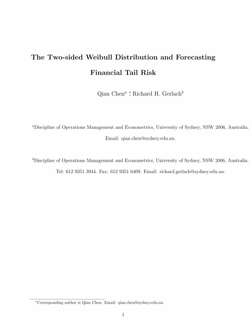
Figure 1 shows some STW densities, and log-densities, for the range of parameter

estimates found for k1 in the real return series we analyse (i.e. k1 ∈ (1, 1.22)), as well

as k1 = 0.95; the skewness was kept constant in each density; the STW distribution’s

flexibility is demonstrated, as is the slight thinning of the tails as k1 > 1.

6

2.2 VaR and tail conditional expectations for two-sided Weibull

The 1-period VaR, for holding an asset, and the conditional 1-period VaR, or ES, are

formally defined via

α = Pr(rt+1 < VaRα|Ωt) ; ESα = E [rt+1|rt+1 < VaRα,Ωt]

where rt+1 is the one-period return from time t to time t + 1, α is the quantile level and

Ωt is the information set at time t. The VaR is thus simply the quantile given in (4).

In practice, λ1k1

is estimated much closer to 0.5 than α, since risk management focuses

on only the extreme tails of returns, particularly the cases α ≤ 0.05, thus only the case

α < λ1k1

in (4) is relevant here. In this context, the tail expectation of an STW is:

ESα1 =

−λ21αbpk1

∫ ∞(−bpV aRα

λ1

)k1(−bpx

λ1

)k1 1k1

+1−1

exp

−(−bpxλ1

)k1 d(−bpxλ1

)k1

=−λ21αbpk1

Γ

1 +1

k1,

(−bpV aRα

λ1

)k1 ; 0 ≤ α <λ1k1

(5)

where Γ(s, x) =∫∞x ts−1e−tdt is the upper incomplete gamma function.

3 Model specification

This section discusses the general forms for the financial return series models considered

in the empirical section. We follow the common assumption that the mean of a return

series is (well approximated as) zero. The generalized model for a financial return series

y is:

yt = (εt − µε)√ht , εt

i.i.d.∼ D(1), (6)

where Var(yt|Ωt) = ht is the conditional variance and D is the conditional distribution

and has variance 1 and mean µε (often 0). The VaR and ES in this model are:

VaRt+1 = D−1α

√ht+1 ; ESt+1 = ESDα

√ht+1. (7)

where D−1α is the inverse cdf of D, and ESDα is the expected shortfall of D, at the α×100%

level. The Gaussian, Student t, Skewed t of Hansen (1994), the AL of Chen et al (2011)

7

and the STW distribution are considered. The latter two have non-zero means that are

subtracted in (6). Expressions for ESDα in the Gaussian and Student-t cases can be found

in McNeil, Frey and Embrechts (2005, pg 45, 46), while for the AL see Chen et al (2011).

Appendix 3 repeats these expressions and contains a derivation of ESDα for the skewed-t

distribution.

3.1 Volatility models

The most general volatility model considered is a two regime smooth transition nonlinear

(ST-)GARCH model, similar to that in Gerlach and Chen (2008). As the data considered

are observed daily, such a smooth change between regimes is potentially more reasonable

than a sharp regime transition, as in a T-GARCH, though both will be considered and

compared. The specified ST-GARCH model has volatility dynamics:

ht = h1t +G(xt−1; ι, r)h2t ,

h[i]t = α

[i]0 + α

[i]1 y

2t−1 + β

[i]1 ht−1. (8)

and thus represents a continuous mixture of two regimes: where h[2]t is the difference

between the conditional variances between the regimes. G(xt−1; γ, r) is a function defined

on [0, 1]: we take a logistic as standard:

G(xt−1; γ, r) =1

1 + exp−γ

(xt−1−rsx

) ,where γ is the smoothness or speed of transition parameter, assumed positive for identifi-

cation; sx is the sample standard deviation of the observed threshold variable x, allowing

γ to be independent of the scale of x.

The T-GARCH model is a special case of (8), where γ → ∞. Further, the GJR-

GARCH is then a special case of the T-GARCH, where xt−1 = yt−1, r = 0 and α[2]0 =

β[2]1 = 0 and G(yt−1|γ = ∞, r = 0) = 1 when yt−1 < 0 and 0 otherwise. The symmetric

GARCH model has constant G(yt−1|γ, r = −∞) = 0, so there is only one regime.

The standard sufficient 2nd order stationary and positivity constraints are:

α[1]0 > 0 ; 0 ≤ α

[1]1 + β

[1]1 < 1 ;α

[1]1 , β

[1]1 ≥ 0;

8

α[1]0 + α

[2]0 > 0 ; 0 ≤ α

[1]1 + 0.5α

[2]1 + β

[1]1 + 0.5β

[2]1 < 1;

α[1]1 + α

[2]1 , β

[1]1 + β

[2]1 ≥ 0;

0 ≤ α[1]1 + α

[2]1 + β

[1]1 + β

[2]1 < 1 (9)

which apply whenever E(G(·)) = 0.5 and D is symmetric. Chen et al (2011) derived

expressions for cp, which replaces 0.5 in these expressions, in the case of the GJR-GARCH

model for the AL distribution. Appendix 2 contains derivations of the extensions of these

expressions to the case of the GJR-GARCH model with STW errors. Expressions are

not known for the T-GARCH or ST-GARCH models in general. However, we note that

with negative skewness, as commonly found in daily financial returns, the values of cp are

> 0.5, indicating that (9) is conservatively sufficient for stationarity.

4 Estimation and Forecasting Methodology

This section specifies the Bayesian methods and MCMC procedures for estimating pa-

rameters and generating forecasts.

4.1 Bayesian estimation methods

In a Bayesian analysis, a likelihood function and a prior are usually required. The required

likelihood follows from the choice of error distribution D and equation (6) together with

a volatility equation (8). We consider the priors for the most general ST-GARCH model

with STW errors.

The ST-GARCH parameters in each regime are grouped and denoted θ[1], θ[2] and each

group is generated separately in the MCMC scheme. Let θ =(θ[1],θ[2]

), the prior is

π(θ[1]) ∝ I(0 < α

[1]0 < s2y, α

[1]1 + β

[1]1 < 1, α

[1]1 , β

[1]1 ≥ 0

);

π(θ[2]|θ[1]) ∝ I

−α[1]0 < α

[2]0 < s2y − α

[1]0 , 0.5(α

[2]1 + β

[2]1 ) < 1− (α

[1]1 + β

[1]1 ),

α[2]0 ≥ −α

[2]1 , β

[2]1 ≥ −β

[1]1 ,−(α

[1]1 + β

[1]1 ) ≤ α

[2]1 + β

[2]1 < 1− (α

[2]1 + β

[2]1 )

,where s2y is the sample variance of the return data. This prior ensures that (9) are satisfied

and that the volatility intercepts are suitably bounded.

9

For the threshold value r a constrained uniform is applied, as standard, i.e. π(r) ∝

I (ll ≤ r ≤ ul); where ll and ul are the 10th and 90th percentiles of the threshold variable,

to ensure sufficient observations for identification and inference in each regime. The prior

for the speed of transition parameter γ is:

π(γ) ∝ I

(− sylog(99)

min(x)− r≤ γ ≤ 20

);

similar to that suggested in Chen, Gerlach, Choy and Lin (2010), which together with

the bounded prior on r ensures that the parameter γ does not get too close to 0, in which

case θ[1] and θ[2] are not identified, since G = 0.5 is constant in that case, while also not

allowing γ → ∞. The prior effectively ensures that the function G is below 0.01 at the

minimum value of the threshold x and thus not constant over the range.

For the STW distribution the parameters λ1 and k1 have a flat prior:

π(λ1) ∝ I (0 < λ1 < k1) ;

The AL distribution has k1 = 1 and the same prior on λ1 = p. For the skewed t

distribution the degrees of freedom and shape parameters, respectively ν and ζ, have:

π(ν) ∝ I (4 < ν < 30) ;π(ζ) ∝ I (−1 < ζ < 1) ;

None of the parameter groupings have a standard recognisable conditional posterior

density and as such Metropolis and Metropolis-Hastings methods are required. Gerlach

and Chen (2008) illustrated the efficiency and speed of mixing gains from employing an

adaptive scheme where iterates in the burn-in period, simulated from standard random

walk Metropolis methods with tuning to achieve desired acceptance rates, are used to

build a Gaussian proposal density for use in the sampling period. Chen et al (2011)

extended this method to cover a mixture of Gaussian proposals, both in the burn-in and

sampling periods. This method is adapted to the models here. This method is a special

simplified case of the more general and flexible ”AdMit” mixture of Student-t proposal

procedure proposed by Hoogerheide, Kaashoek and van Dijk (2007).

Convergence is obsessively checked for by running the MCMC scheme from multiple

and wide ranging starting points and checking trace plots of iterates for convergence to

the same posterior. Simulation results are available from the authors on request.

10

4.2 VaR and ES forecasts

One-step-ahead forecasting is considered. The GARCH family in (8) provides one-step-

ahead forecasts of volatility based on known parameter values. In MCMC methods, at

each stage the entire parameter vector, denoted θ, has values simulated for it from the

posterior, combining to give a Monte Carlo sample θ[1], . . . ,θ[N ], where N is the MC

sample size. Each of these iterates provides a one-step-ahead forecast of ht, which can be

combined with, (7) via e.g. (4) and (5) for STW errors, to give MC iterate forecasts of

VaR and ES, i.e. VaR[i], ES[i] for i = 1, . . . , N , for each model. These are simply averaged

over the iterates in the sampling period of the MCMC scheme, to give a one-step-ahead

forecast of VaR and ES for each model.

4.3 Back-testing VaR models

As recommended by Basel II VaR forecasts are obtained at the 1% risk level, while also

5% is considered for illustration. Each model’s forecasts are evaluated and compared by

first considering their violation rate:

VRate =1

m

n+m∑t=n+1

I(yt < VaRt),

and comparing their violation ratios VRate/α, where VRate/α ≈ 1 is preferred. Formal

back-tests considered are the unconditional coverage (UC) test of Kupiec (1995); the

conditional coverage (CC) test of Christoffersen (1998) and the Dynamic Quantile (DQ)

test of Engle and Manganelli (2004).

4.4 Back-testing ES models

Although there are a few existing back-testing methods in the literature for ES, e.g., the

censored Gaussian method of Berkowitz (2001), the functional delta approach of Kerkhof

and Melenberg (2004) and the saddle point techniques of Wong (2008), they appear to be

based on Gaussian distribution, and also seem overly-complex and difficult to implement.

Kerkhof and Melenberg (2004) made an excellent suggestion of comparing ES models in

the same manner as VaR models: on an equal quantile level. ES after all does occur at

11

a specific quantile of the return distribution. In particular, for the standard Gaussian

and AL distributions, the ES quantile level at a fixed α is (different but) constant: the

ES quantile level only depends on α for the Gaussian and AL (and not on the unknown

shape parameter of the AL). Denote δESα as the nominal levels for ES at VaR level α. For

the Gaussian and AL distribution, these are given in Table 1.

Chen et al (2011) exploited this result to employ the standard VaR back-testing

methods, discussed above, to back-test ES models. For the Student-t and skewed-t,

however, the quantile level of ES depends on α, plus the degrees of freedom ν and λ for

the skewed-t. Similarly, for the STW, the ES quantile level depends on the parameters

λ1, k1. To back-test ES models with these distributions, we approximate by considering

the ES level for the average estimated parameters during the forecast sample. This works

well since these parameters do not change very much during the forecast period.

5 Empirical study

5.1 Data

The model is illustrated by applying it to daily return series from four international

stock market indices: the S&P 500 (US); FTSE 100 (UK); AORD All ordinaries index

(Australia); HANG SENG Index (Hong Kong); plus two exchange rate series: the AU

dollar to the US dollar and the Euro to the US dollar; as well as one single asset series:

IBM. The data are obtained from Yahoo! Finance, covering twelve years, January 1998 to

January 2010, except the exchange rate of Euro to US dollar, which starts from January

1999. The daily return series is yt = (ln(Pt) − ln(Pt−1)) × 100, where Pt is the closing

price/value on day t.

The sample is initially divided into two periods: the period from January 1998 to

December 2005, roughly the first 2000 returns, is used as an initial learning period. The

data from January 2006 to January 2010 are used as the forecasting period. The forecast

sample sizes vary from 770 to 1050 days, due to different trading day holidays, etc. and

this period completely contains the GFC. Table 2 shows summary statistics for the seven

12

return series in the learning and forecast samples. Clearly, that the forecast period is

mostly more volatile and more fat-tailed (higher kurtosis), except notably for IBM. The

estimation results in each series, not shown to save space, are mostly as expected and well-

documented in the literature: high volatility persistence (α1 + β1); fat-tailed (e.g. ν < 10

in Student-t and skewed-t error models) and mildly negatively skewed (e.g. λ1/k1 > 0.5

in STW, p > 0.5 in AL and λ < 0 in skewed-t) conditional distributions.

5.2 VaR forecast comparison

Table 3 shows the ratios, and their summaries, of observed VRates to the true nominal

levels α = 0.01, 0.05 across all series; summaries shown are average (’Mean’) and deviation

(’Std’) for each model and series. ’Std’ is the square root of the average squared distance

of the observed ratio away from the expected ratio of 1. For each series, the ratio closest to

1 is boxed, while the mean ratio and deviation closest to 1 over the models, for each series,

is also boxed. Violation ratios that are significantly different from 1, at a 5% significance

level by the UC test, are in bold.

First, it is clear that the differences between models are dominated by the choice of

error distribution: models with the same distribution but different volatility equation are

much closer in violation ratios, to each other, than they are to models with a different

distribution. Thus models with the same error distributions appear together in the table.

As such, discussion centres on the different distributions first. At α = 0.01, it is clear

that models with Gaussian errors are consistently anti-conservative and under-predict risk

levels in all series: on average VRates are double or more the nominal 1%. Alternatively,

models with AL errors over-predict risk levels: on average VRates are half the nominal

1%, and are thus conservative; this agrees with results in Chen et al (2011). Models

with skewed-t errors tend to under-predict risk, but less so than Gaussian models, with

average VRates about 20-30% too high. Models with Student-t and STW errors are

clearly the best performed and most favoured with VRates close to nominal on average.

The GJR-t model ranks highest with average VRate closest to 1 (1.02), closely followed

by the GARCH-STW with 1.03, which also has the minimum deviation from 1 (0.3),

equal best with the ST-GARCH-STW model. All models with STW errors have VRate

13

ratio deviations equal to or lower than all other models. Informally, then, models with

STW errors have done best in forecasting risk levels at α = 0.01, very marginally ahead

of models with Student-t errors.

Similar results hold for α = 0.05, with Gaussian and skewed-t error models con-

sistently under-predicting risk, while models with AL, Student-t and STW errors have

VRate ratios quite close to 1 across the seven series.

Table 4 shows counts of the number of rejections for each model, at a 5% significance

level, across the seven series, under the three formal back-tests: the unconditional coverage

(UC), the conditional coverage (CC), and the dynamic quantile (DQ) test. Following

Engle and Manganelli (2004) we choose a lag of 4 for the DQ test, while using the extended

CC test in Chen et al (2011), also with a lag of 4. At α = 0.01 the Gaussian error models

are rejected in all or most series, while the models with Student-t errors are rejected

on average more than the other models. The three best models are rejected only in

one series: the GJR-GARCH-STW, and the ST-GARCH and GJR-GARCH both with

skewed-t errors. Models with AL, skewed-t and STW errors are quite comparable and do

the best on these tests across the seven series. At α = 0.05, models with Gaussian errors

are again rejected in most series. The other models are quite comparable, except for the

GJR-GARCH-STW and T-GARCH-STW models, which are only rejected in one series

each.

In summary, models with STW and Student-t errors tended to have average VRates

closest to nominal at both α = 0.01, 0.05. In terms of deviation in VRate ratios from

1, again models with STW errors did best overall, though models with AL errors did

very well at α = 0.05. In terms of the tests, for both α = 0.01, 0.05 a model with

STW had the minimum number of rejections: one in seven series. Models with Gaussian

errors significantly under-predicted risk in most series at α = 0.01, 0.05 by over 100% at

α = 0.01; models with skewed-t errors, while doing reasonably well in the formal tests,

under-predicted risk levels by 10− 30% on average.

14

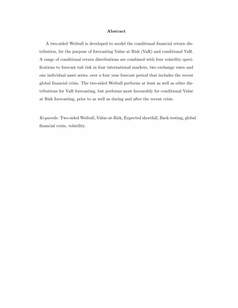
5.3 Expected Shortfall Forecast Comparison

The ES forecasts from several parametric models, for the returns on the Australian stock

market and the AU to US dollar exchange rate, are shown in Figure 2.

The plots indicate a clear ordering in ES levels across distributions: the Gaussian is

least extreme, followed by the Student-t, skewed-t, STW, while the AL distribution gives

the most extreme ES forecasts. This pattern occurred consistently across the seven series,

holding the volatility model constant.

The quantile levels that ES occurs at, for various VaR quantile levels α, are well known

and calculable in standard software for the Gaussian and Student-t distributions, using

their cdf functions; the ES quantile levels, constant for fixed α, for the AL distribution

were derived by Chen et al (2011) and are given in appendix 3 and Table 1. The closed

forms for the ES and the relation between ES and VaR for the skewed-t are derived and

given in appendix 3, while for the STW this is given by (5) and (3) allows evaluation of

the ES quantile level for a STW at VaR level α. Table 5 shows the approximate quantile

levels for ES from the Student-t, skewed-t and STW models, with ST-GARCH volatility

equation, obtained using the average of the estimates of each distribution’s parameters

over the forecast period in each series. The quantile levels for other volatility models are

very similar and not shown to save space.

Using these ES quantile levels, the ES violation rate, ESRate, is defined as:

ESRate =1

m

n+m∑t=n+1

I(yt < ESt),

and a good model should have ESRate very close to the nominal δα.

Table 6 contains the ratios of δα/δα at α = 0.01, 0.05 across all models and the seven

series in the forecast period. Again the best risk ratio, closest to 1, is boxed and ESRates

significantly different to nominal by the UC test are in bold. At α = 0.01, it is clear that

models with Gaussian errors are consistently anti-conservative and significantly under-

predict risk levels in all series: on average ESRates are close to 3 times or more the nominal

1%. Further, models with Student-t errors also under-predict risk, sometimes significantly,

on average their ES violation rates are 55 − 84% above nominal. Alternatively, models

15

with AL errors again over-predict risk levels, but not significantly, on average ESRates are

half the nominal 1%, and are thus conservative; agreeing with Chen et al (2011). Models

with skewed-t errors tend to under-predict risk, not significantly, with ESRates 16-39%

too high on average. However the 3rd and 4th ranked models, by average ESRate ratio,

with 1.16 and 1.17 respectively, are the GARCH and GJR-GARCH with skewed-t errors.

The top two ranked models by average ESRate ratio, with 1.02 and 1.05, are the GARCH

and T-GARCH with STW errors. The GJR-GARCH and ST-GARCH with STW rank

5th and 6th respectively on this measure. Further, by minimum deviation of ratios from

1, the models with STW errors rank 1st, 2nd, 3rd, with the ST-GARCH-STW ranking

5th best. The 4th ranked model is the GJR-GARCH with skewed-t errors. Under these

criteria, it is clear that models with STW errors have performed most favourably, followed

by the GARCH and GJR-GARCH with skewed-t errors.

At α = 0.05, a similar story now holds. Models with Gaussian errors are signifcantly

anti-conservative, but now by ≈ 50−70% on average, and Student-t error models perform

similarly and are mostly rejected in 3 of the 7 series by the UCC test. Models with AL

errors now only marginally over-predict risk levels, with ESRates on average 15 − 20%

below nominal, while Skewed-t error models under-predict risk levels again by 17− 30%

on average. Here, the top four ranked models, with ESRates clearly closest to nominal

on average, are the four STW error models. Three of these, excluding the GJR-GARCH-

STW, occupy the top ranked positions by minimum deviation in ratios from 1.

Table 4 shows counts of the number of rejections for each ES forecast model, at

a 5% significance level, across the seven series, under the three formal back-tests: the

unconditional coverage (UC), the conditional coverage (CC), and the dynamic quantile

(DQ) test using the ES quantile levels discussed above. At α = 0.01 and 0.05 the Gaussian

error models are again rejected in all or most series by all tests, while the models with

Student-t errors are again rejected on average more than the other models. At α = 0.05,

Student-t error models are rejected in all or most series for ES forecasting. The two best

models could not be rejected in any series: the T-GARCH-AL and the GJR-GARCH-

STW. Models with AL, STW and skewed-t errors were generally rejected in 1 series only

at α = 0.01, and thus do quite comparably on these tests across the seven series. At

16

α = 0.05, only the GJR-GARCH with STW errors could not be rejected in any series; all

other models were rejected at least twice.

Overall, for forecasting ES during this forecast period, models with STW errors have

performed more favourably than all other models and error distributions considered, with

ESRates generally closest to nominal in both average and squared deviation and ES

forecasts mostly not rejected by the formal tests, across the seven return series. Under

each criteria, a model with STW errors ranked first. The models with AL errors may also

be attractive for regulatory purposes, since they have very small violation ratios, basically

half the amount of violations expected. However, these smaller violation ratios do signal

over-estimation of risk and excessive allocation of capital, which may not be ideal. Models

with STW errors provided adequate and accurate risk coverage.

5.4 Pre-financial-crisis and post-financial-crisis forecast perfor-

mance

The forecast sample period covers the well-known GFC. The performance of the models

may vary between the pre-financial-crisis effects period and the post-financial-crisis period

(which contains returns during the GFC and post-crisis). We thus present the pre and

during/post-crisis comparison of the models’ risk forecasting performance.

A specific date for the start of the crisis must be chosen here, but this date need

not be exactly the same in each market. From news media accounts and Wikipedia,

it is largely agreed that the effects of the crisis are initially apparent during September

and/or October, 2008 in international markets. We choose dates for each market based

on maximizing the sample return variance in the post-crisis period among possible days in

September/October 2008. The dates thus chosen for each market were: Australia, 22nd

September; US and IBM, 19th September; UK, 10th September; HK, 18th September;

AU/US, 23rd September; and EUR/US, 23rd September, all in 2008. The forecast sample

up to the day before these dates is the pre-crisis period, while from these dates up to

January, 2010, is the post-crisis period. For each market, there are approximately 700

days in the pre-crisis period and approximately 350 days in the post-crisis sample.

17

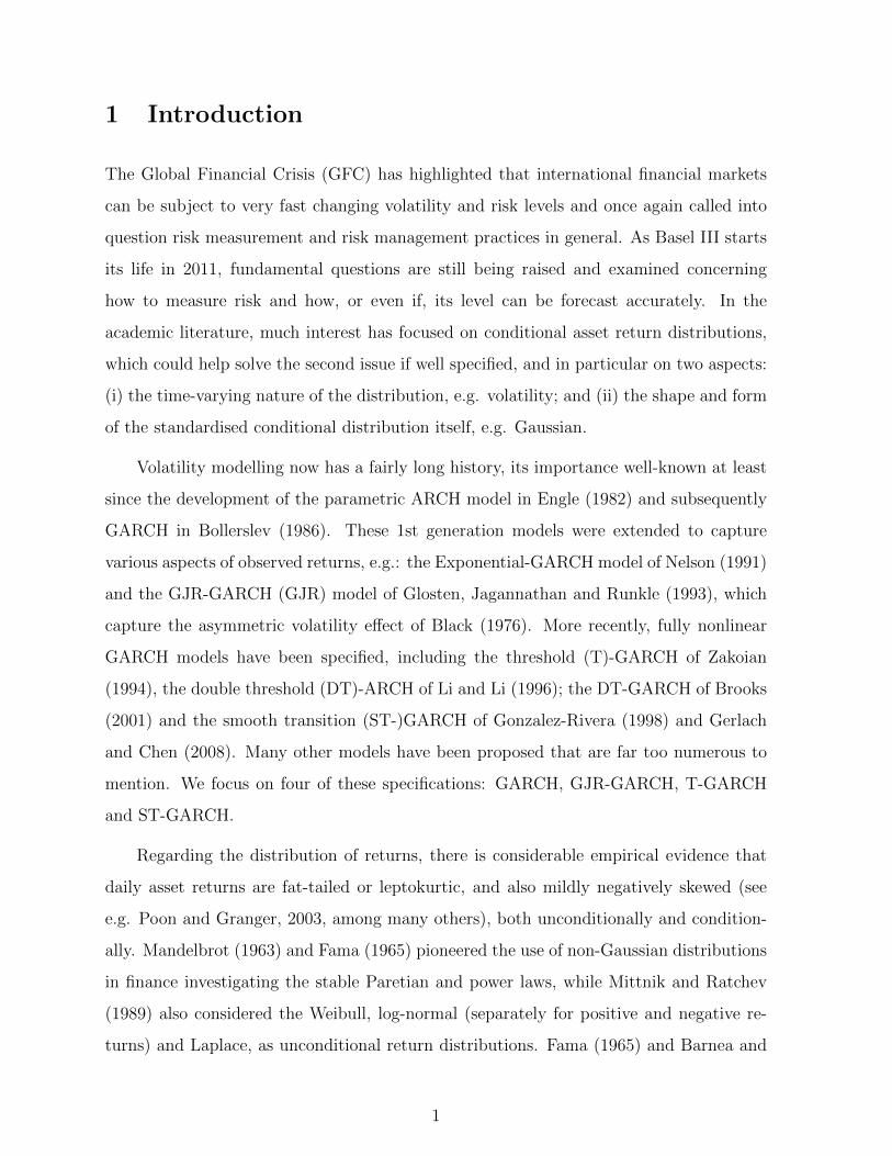
Figures 3 and 4 show the ratios of VRate/α and ESRate/δα at α = 0.01, 0.05 for the

pre-crisis and post-crisis periods for the VaR and ES forecast models, as labelled. The

results for the pre-crisis sample are highly consistent with those for the whole forecast

sample, no doubt influenced by the larger overlapping sample size: Models with STW

and Student-t errors forecast VaR most accurately at the 1% and 5% risk levels, with

VRate averaging close to 1, though STW error models have VRate ratios with slightly

lower variation around 1. Further, only models with STW errors have ESRate ratios con-

sistently, and averaging, close to 1. Models with AL errors are again the only consistently

conservative risk forecasters for both VaR and ES.

Results for the post-crisis period tell a slightly different story. For VaR forecasting,

models with Student-t, skewed-t and STW errors perform well at α = 0.01, all with

average ratios close to 1 and similar deviations about 1, across the seven series. For ES

forecasting, the TW is clearly the best model post-crisis, with average ratio closest to

1 and smallest deviation about 1. At the 5% risk level however, the models with AL

and Student-t errors perform best for VaR forecasting, with STW models slightly under-

predicting risk levels on average. For ES forecasting at α = 0.05, the TW has the closest

average ratio to 1 post-crisis, but the AL also does well and has the smallest deviation in

ratios from 1.

5.5 Loss function

Loss functions are also applicable to assess quantile forecasts. The applicable loss function

is the criterion function, minimised in quantile regression estimation e.g. as in Koenker

and Bassett (1978), as can be written as:

LF =n+m∑t=n+1

(yt −Rt) (α− It).

where It is the indicator variable of a violation (i.e. yt < Rt), Rt is the risk forecast, here

we use V aRt for each model/method, and α is the quantile where the VaR is evaluated.

ES forecasts can also be assessed at their approximate quantile levels, whereby δα is

substituted for α above. The best risk forecasts in terms of accuracy should minimise this

loss function.

18

Figure 5 shows the mean of the loss function for the VaR and ES forecasts via various

models, taken over the seven series in the entire forecast period. Two things are apparent:

the GJR model (shown as squares) usually has the lowest average loss for each error

distribution; for VaR forecasting at α = 0.01, models with Student-t, skewed-t and STW

errors have the lowest, and comparable, average losses. For VaR forecasting at α = 0.05

however, the skewed-t, AL and STW-error models have comparable and lowest average

loss. For ES, losses among all distributions except the Gaussian, which has the largest

average loss in each case, seem quite close and comparable.

Overall, the STW model is the most favourably performed risk forecaster for this

forecast data period across the seven series over both VaR and ES forecasting at both

α = 0.01, 0.05 levels. By almost all criteria, models with STW errors ranked best or

equal best, with violation rates closest to 1 by average and squared deviation, minimum

number of model rejections by formal tests, both in the entire period and in the pre and

post-GFC periods. Models with Student-t errors consistently did well at VaR forecasting

for α = 0.01, while models with AL errors were consistently conservative and exhibited

violation rates usually below nominal, with comparatively small variation in violation rate

ratios.

6 Conclusion

The recent global financial crisis challenges market participators’ ability to provide reason-

able coverage for dynamic changing risk levels. As a coherent risk measurement method,

expected shortfall is able to measure the size of loss in extreme cases, unlike VaR. De-

spite the benefit of this alternative method, expected shortfall is absent in regulations

such as Basel II, perhaps mostly because back-testing of ES models is less straightforward

than that for VaR. Calculating a benchmark for allocating regulatory capital and thus

protecting the financial institutions from the risk during extreme market movements is

the ultimate goal of VaR and ES models. However, as another essential function of these

financial entities is to make profit, the allocation of capital matters a lot. In this paper,

we argue that other than using an extremely conservative model, a more appropriate

19

approach should be able to relieve the burden of over-allocation of regulatory capital,

and protect against the risky under-allocation of capital, by more accurately forecasting

dynamic risk levels, thus carefully and properly increasing the investment opportunities

in more profitable assets. For this purpose, we proposed the use of a two-sided Weibull

conditional return distribution, coupled with a volatility model. Properties of this distri-

bution were developed and presented, including the VaR and expected shortfall functions.

An adaptive Markov chain Monte Carlo method was employed for estimation and forecast-

ing. An empirical study of seven asset return series found that models with conditional

two-sided Weibull errors were highly accurate at forecasting both VaR and ES levels and

could not be consistently rejected or bettered across several criteria, compared to the

Gaussian, Student-t, skewed-t and asymmetric Laplace conditional return distributions.

This accurate performance was found to hold both before the GFC hit markets as well

as during and after the GFC period. Hopefully, the model introduced in this paper offers

both the regulators and the financial institutions a new option or compromise between

suffering from excess violations or from unnecessarily reduced profit. It is clear that the

two-sided Weibull has improved modelling the tails of the conditional return distribution.

An extension of our model could involve allowing a distribution that had Weibull tails

while preserving a single mode, perhaps through the use of a partitioned distribution: e.g.

Student-t in the centre and Weibull in the tails.

Appendices

Appendix 1 Some properties of STW

Let X ∼ STW(λ1, k1). Then,

E(X) =−λ21bpk1

Γ(

1 +1

k1

)+

λ22bpk2

Γ(

1 +1

k2

)= µX . (10)

The skewness of a standardized two-sided Weibull random variable is

S(X) = − λ41b3pk1

Γ(

1 +3

k1

)+

λ42b3pk2

Γ(

1 +3

k2

)

20

− 3

[λ31b2pk1

Γ(

1 +2

k1

)+

λ32b2pk2

Γ(

1 +2

k2

)] [− λ21bpk1

Γ(

1 +1

k1

)+

λ22bpk2

Γ(

1 +1

k2

)]

+ 2

[− λ21bpk1

Γ(

1 +1

k1

)+

λ22bpk2

Γ(

1 +1

k2

)]3. (11)

The kurtosis of a standardized two-sided Weibull random variable is

K(X) =λ51b4pk1

Γ(

1 +2

k1

)+

λ52b4pk2

Γ(

1 +2

k2

)

− 4

[− λ21bpk1

Γ(

1 +1

k1

)+

λ22bpk2

Γ(

1 +1

k2

)] [−λ41b3pk1

Γ(

1 +3

k1

)+

λ42b3pk2

Γ(

1 +3

k2

)]

+ 6

[− λ21bpk1

Γ(

1 +1

k1

)+

λ22bpk2

Γ(

1 +1

k2

)]2 [λ31b2pk1

Γ(

1 +2

k1

)+

λ32b2pk2

Γ(

1 +2

k2

)]

− 3

[− λ21bpk1

Γ(

1 +1

k1

)+

λ22bpk2

Γ(

1 +1

k2

)]4(12)

These formulas can be used to verify the range of skewness and kurtosis given in Section

2 for the STW.

Appendix 2 A necessary and sufficient condition for second-order stationarity of the

GJR-GARCH-STW model

The GJR-GARCH-STW model is:

yt = εtσt,

εti.i.d.∼ STW (λ1, k1),

ht = α0 + (α1 + α2I(yt−1 < 0)) y2t−1 + β1ht−1. (13)

Theorem: A necessary and sufficient condition for the the existence of a second-order

stationary solution to the GJR-GARCH-STW model is:

α1 + β1 + α2cp < 1, (14)

where

cp =

µ2ελ1k1

exp[−(−bpµελ1

)k1]+ 2

µελ21bpk1

Γ(1 + 1

k1, µε

)+

λ31b2pk1

Γ(1 + 2

k1, µε

); if 0.5 ≤ λ1

k1≤ 1

µ2εk1−λ1k1

exp[−(−bpµεk1−λ1

)k1]+ 2µε(k1−λ1)

2

bpk1γ(1 + 1

k1, µε

)+ (k1−λ1)3

b2pk1γ(1 + 2

k1, µε

)+µ2

ελ1k1

+ 2µελ21bpk1

Γ(1 + 1

k1

)+

λ31b2pk1

Γ(1 + 2

k1

); if 0 ≤ λ1

k1≤ 0.5

21

Here bp =

√λ31k1

Γ(1 + 2

k1

)+

λ32k1

Γ(1 + 2

k1

)−[−λ21k1

Γ(1 + 1

k1

)+

λ22k1

Γ(1 + 1

k1

)]2, µε =

−λ21bpk1

Γ(1 + 1

k1

)+

λ22bpk1

Γ(1 + 1

k1

)and λ2 = k1 − λ1. Γ (s, x) is the upper incomplete gamma function and

γ (s, x) is the lower incomplete gamma function. If λ1k1

= 1/2, the above incomplete

gamma functions become gamma functions, and if k1 = 1, then cp = 1/2: i.e. in this sym-

metric error case, the necessary and sufficient condition reduces to that of the traditional

GJR-GARCH specification.

Proof: First note from (13) with STW errors that Iyt−1<0 = Iεt−1<µε, and

σ2t = α0 + (α1 + α2Iεt−1<µε)(εt−1 − µε)2σ2

t−1 + β1σ2t−1 (15)

= α0 + ϕt−1σ2t−1 ,

where ϕt = (α1 + α2Iεt<µε)(εt − µε)2 + β1.

We first prove the necessity. Assume yt is a second-order stationary solution to the

GJR-GARCH-TW model. Then E(y2t ) = E(σ2t ) < ∞, which is independent of t. It

follows from (13) together with (15) and Var(εt) = E[(εt−1 − µε)2] = 1 that

E(y2t ) = E(σ2t ) = α0 + E(ϕt−1σ

2t−1) = α0 + E(ϕt−1)E(σ2

t−1)

= α0 + E(ϕt)E(σ2t )

=α0

1− E(ϕt),

by the independence of εt and σt in (13). Therefore Eϕt−1 < 1 for α0 > 0 and Eσ2t > 0.

E(ϕt) = α1 + β1 + α2E(Iεt<µε(εt − µε)2

)(16)

= α1 + β1 + α2cp .

To show this, note that:

E(Iεt<µε(εt − µε)2

)=∫ µε

−∞(x− µε)2f(x|p) dx , (17)

where f(x|p) is the STW density function given by (1). For λ1k1< 0.5 we have µε > 0, so

that

E(Iεt<µε(εt − µε)2

)=

∫ µε

0(x− µε)2bp

(bpx

λ2

)k1−1exp

−(bpxλ2

)k1 dx (18)

+∫ 0

−∞(x− µε)2bp

(−bpxλ1

)k1−1exp

−(−bpxλ1

)k1 dx ,22

while for λ1k1> 0.5 we have µε < 0, so that

E(Iεt<µε(εt − µε)2

)=∫ µε

−∞(x− µε)2bp

(−bpxλ1

)k1−1exp

−(−bpxλ1

)k1 dx , (19)

where in each case integration by parts applied twice results in (15).

We now turn to sufficiency. Under the condition (14), note from (15) that through

iterations, we find that

σ2t = α0 + α0

∞∑j=1

j∏i=1

ϕt−j. (20)

Obviously, owing to the i.i.d. property of εt in (6), (20) is a second-order stationary

solution to (15) if we can display

E(σ2t ) = α0 + α0

∞∑j=1

E

j∏i=1

ϕt−j

= α0 + α0

∞∑j=1

(E(ϕt))j <∞. (21)

This is seen to hold true on noticing (16) and (14). Hence it follows from (13) that there

is a stationary solution to the model in (13) under (14).

Appendix 3 The VaR and ES of the skewed student’s t and AL

The skewed student’s t distribution by Hansen (1994) is considered and has the

following density function:

g(z|ν, ζ) =

bc(

1 + 1ν−2

(bz+a1−ζ

)2)−(ν+1)/2

; z < −a/b,

bc(

1 + 1ν−2

(bz+a1+ζ

)2)−(ν+1)/2

; z ≥ −a/b

where 2 < ν <∞, and −1 < ζ < 1. The constants a, b and c are given by

a = 4ζc(ν − 2

ν − 1

),

b2 = 1 + 3ζ2 − a2,

c =Γ(ν+12

)√φ(ν − 2)Γ

(ν2

) . (22)

The variable is positively skewed to the right when ζ > 0, and negatively skewed when

ζ < 0. The inverse CDF of the skewed student’s t distribution Skewt(ν, λ) is:

F−1(α|ν, ζ) =

1−ζb

√ν−2νF−1s

(α

1−ζ , ν)− a

b; α < 1−ζ

2,

1+ζb

√ν−2νF−1s

(0.5 + 1

1+ζ

(α− 1−ζ

2

), ν)− a

b; α ≥ 1−ζ

2,

23

Here F−1s is the inverse CDF of the Student’s t distribution.

The Expected Shortfall of a Skewt(ν, ζ) at level α for a long position can be calibrated

via:

ESα =− c(1−ζ)2

bν−2ν−1d

ν−12 − 1−ζ

bF−1s

(bV aRα+a

1−ζ , ν)

α; V aRα < −

a

b(23)

where

d = cos2(arctan

(− bV aRα + a

(1− ζ)√ν − 2

))

The Asymmetric Laplace (AL) distribution is simply the STW distribution with

k1 = 1. All formulas,. e.g. VaR and ES, for the AL can be obtained by setting k1 = 1

and using the corresponding formula for the STW. For example, if p = λ1, then:

V aRα,t+1 = σt+1p

bplog

(α

p

)− µεσt+1,

ESα,t+1 =

1− 1

log(αp

)VaRα,t+1 ; 0 ≤ α < p. (24)

References

Aas K. and Haff I. (2006), “The Generalized Hyperbolic Skew Student’s t-Distribution,”

Journal of Financial Econometrics, 4, 275-309.

Artzner, P., Delbaen, F., Eber, J.M., and Heath, D. (1997), “Thinking coherently,”Risk,

10(11), 68-71.

Artzener, P., Delbaen, F., Eber, J.M., and Heath, D. (1999), “Coherent measures of

risk,”Mathematical Finance, 9, 203-228.

Bakshi, G. and Panayotov, G. (2007), “The Capital Adeqacy Puzzle,” working paper,

Smith Business School, University of Maryland.

Barnea, A. and Downes, D. H. (1973), “A re-examination of the empirical distribution of

stock price changes,” Journal of the American Statistical Association, 168, 348-50.

24

Berkowitz, J. (2001), “Testing density forecasts, with applications to risk management,”

Journal of Business and Economic Statistics, 19, 465-474.

Black, F. (1976), “Studies in stock price volatility changes,” American Statistical Asso-

ciation Proceedings of the Business and Economic Statistics Section, 178-181.

Brooks, C. (2001), “A double-threshold GARCH model for the French France/Deutschmark

exchange rate,” Journal of Forecasting, 20, 135-145.

Bollerslev, T. (1986), “Generalized autoregressive conditional heteroskedasticity,” Jour-

nal of Econometrics, 31, 307-327.

Bollerslev, T. (1987), “A conditionally heteroskedastic time series model for speculative

prices and rates of return,” Review of Economics and Statistics, 69(3), 542-547.

Chen, C.W.S.,Gerlach, R. and Lin, E.M.H. (2008), “Volatility forecasting using threshold

heteroskedastic models of the intra-day range,” Computational Statistics & Data

Analysis, 52(6), 2990-3010.

Chen, Q., Gerlach, R. and Lu, Z. (2011), “Bayesian Value-at-Risk and expected shortfall

forecasting via the asymmetric Laplace distribution,” Computational Statistics &

Data Analysis, in press.

Chen, Y.T. (2001), “Testing conditional symmetry with an application to stock returns,”

working paper, Institute for Social Science and Philosophy, Academia Sinica.

Christoffersen, P. (1998), “Evaluating interval forecasts,” International Economic Re-

view, 39, 841-862.

Engle, R. F. (1982), “Autoregressive conditional heteroskedasticity with estimates of the

variance of United Kingdom inflations,” Econometrica, 50, 987-1007.

Engle, R.F. and Russell, J. (1998), “Autoregressive Conditional Duration: A New Model

for Irregulatory Spaced Transaction Data,” Econometrica, 66, 1127-1162.

Engle, R. F. and Manganelli, S. (2004), “CAViaR: conditional autoregressive value at risk

by regression quantiles,” Journal of Business and Economic Statistics, 22, 367-381.

25

Ewerhart, C. (2002), “Banks, internal models and the problem of adverse selection,”,

working paper, University of Bonn.

Fama, EUGENE F. (1965), “Portfolio Analysis in a Stable Paretian Market,” Manage-

ment Science .

Gerlach, R., Chen, C.W.S. (2008), “Bayesian inference and model comparison for asym-

metric smooth transition heteroskedastic models,” Statistics and Computing, 18 (4),

391-408.

Glosten, L. R., Jagannathan, R., and Runkle, D. E. (1993), “On the Relation Between

the Expected Value And the Volatility of the Nominal Excess Return on Stock,”

Journal of Finance, 48, 1779-1801.

Gonzalez-Rivera, G. (1998), “Smooth Transition GARCH Models,” Studies in Nonlinear

Dynamics and Econometrics, 3(2), 61-78.

Griffin, J.E. and Steel, M.F.J. (2006), “Order-Based Dependent Dirichlet Processes,”

Journal of the American Statistical Association, 101, 179-194.

Hansen, B. E. (1994), “Autoregressive Conditional Density Estimation,” International

Economic Review, 35(3), 705-730.

Hinkley, D.V. and Revankar, N.S. (1977), “Estimation of the Pareto law from underre-

ported data,” Journal of Econometrics, 5, 1-11.

Hoogerheide, L.F., van Dijk, H.K. (2007), “On the shape of posterior densities and credi-

ble sets in instrumental variable regression models with reduced rank: an application

of flexible sampling methods using neural networks,” Journal of Econometrics, 5,

1-11.

Jensen, M. J. and Maheu, J. M. (2010), “Bayesian semiparametric stochastic volatility

modeling”, Journal of Econometrics, 157(2), 306 - 316.

Kerkhof, F.L.J. and Melenberg, B. (2004), “Backtesting for risk-based regulatory capi-

tal,” Journal of Banking and Finance, 28, 1845-1865.

26

Koenker, Roger W. and Bassett, Gilbert. Jr. (1978), “Regression Quantiles,” Econo-

metrica, 46(1), 33-50.

Kupiec, P. H. (1995), “Techniques for verifying the accuracy of risk measurement mod-

els,” The Journal of Derivatives, 3, 73-84.

Li, C.W. and Li, W.K. (1996), “On a double-threshold autoregressive heteroscedastic

time series model,” Journal of Applied Economics, 11, 253-274.

Liu, Shi-Miin and Brorsen, B. Wade (1995), “GARCH-Stable as a Model of Futures

Price Movements,” Review of Quantitative Finance and Accounting, 5(2), 155-67.

Malevergne, Y. and Sornette, D. (2004), “VaR-Efficient portfolios for a class of super

and sub-exponentially decaying assets return distributions”, Quantitative Finance,

4, 17-36.

Mandelbrot, B. (1963), “The Variation of Certain Speculative Prices,” Journal of Busi-

ness, University of Chicago Press, 36, 394.

McCulloch, J. Huston (1985), “Interest-Risk Sensitive Deposit Insurance Premia,” Jour-

nal of Banking and Finance, 9, 137-156.

McNeil, A.J., Frey, R., Embrechts, P. (2005), “Quantitative Risk Management”, New

Jersey: Princeton University Press, p. 283.

Mittnik, M. and Rachev, S.T. (1989), “Stable distributions for asset returns,” Applied

Mathematics Letters, 2(3), 301-304.

Nelson, W. (1982), “Applied life data analysis”, John Wiley and Sons, New York.

Nelson, D. B. (1991), “Conditional heteroskedasticity in asset returns: a new approach

econometrica,” Econometrica, 59, 347-370.

Poon, S. H. and Granger,C. (2003), “Forecasting volatility in financial markets: A re-

view,” Journal of Economic Literature, 41, 478-539.

Richardson, M. and Smith, T. (1993), “Asymptotic filtering theory for univariate ARCH

models,” Journal of Financial and Quantitative Analysis, 24(2), 205-216.

27

Sornette, D., Simonetti, P. and Andersen, J.V. (2000b), “Φq-field theory for portfolio

optimization : fat-tails and non-linear correlations,” Physics Reports, 335(2), 19-

92.

Vlaar, P. J. G. and Palm, F. C. (1993), “The Message in Weekly Exchange Rates in

the Eu- ropean Monetary System: Mean Reversion, Conditional Heteroskedasticity,

and Jumps,” Journal of Business and Economic Statistics, 11, 351-360.

Weibull, W. (1951), “A statistical distribution function of wide applicability,” Journal

of Applied Mechanics -Trans. ASME, 18, 293-297.

Wong, K. (2008), “Backtesting trading risk of commercial banks using expected short-

fall,” Journal of Banking and Finance, 32, 1404-1415.

Zakoian, J.M. (1994), “Threshold heteroscedastic models,” Journal of Economic Dy-

namics and Control, 18, 931-944.

Zhu, D., Galbraith, J. (2009), ”Forecasting expected shortfall with a generalized asym-

metric Student-t distribution,” CIRANO Working Papers, 2009s-24, CIRANO.

Tables and Figures

Table 1: ES quantile levels for corresponding VaR level αδα

α N(0, 1) AL

0.01 0.0038 0.0037

0.05 0.0196 0.0184

28

STW densities

STW log-densities

Figure 1: Some standardised two-sided Weibull densities.

29

Australian market.

AU/US.

Figure 2: 1% ES forecasts from GJR-n,GJR-t,GJR-skt,GJR-ALCP and GJR-TW.

30

Figure 3: Circles: GARCH; squares: GJR; crosses: TGARCH; diamonds: STGARCH;

large triangles: mean of VRates for each distribution.

Figure 4: Circles: GARCH; squares: GJR; crosses: TGARCH; diamonds: STGARCH;

large triangles: mean of ESRates for each distribution.

31

Table 2: Summary statistics

Index Period Mean Std Skewness Kurtosis Min Max

Aus 98-05 0.028 0.73 -0.53 7.12 -5.85 3.39

06-09 0.007 1.36 -0.54 7.23 -8.55 5.36

US 98-05 0.013 1.20 0.00 5.36 -7.04 5.57

06-09 -0.011 1.65 -0.22 11.44 -9.47 10.96

UK 98-05 0.003 1.20 -0.11 5.19 -5.59 5.90

06-09 -0.001 1.53 -0.10 10.00 -9.26 9.38

HK 98-05 0.019 1.64 0.20 8.64 -9.29 13.40

06-09 0.033 2.13 0.09 9.26 -13.58 13.41

AU/US 98-05 0.006 0.72 -0.19 5.53 -4.45 4.82

06-09 0.022 1.13 -0.72 15.10 -8.21 7.70

EUR/US 98-05 0.006 0.61 0.02 3.72 -2.47 2.71

06-09 0.010 0.74 0.39 7.36 -3.00 4.62

IBM 98-05 -0.012 2.677 -9.449 253.415 -71.130 12.364

06-10 0.044 1.623 0.177 7.681 -6.102 10.899

Figure 5: Loss function of VaR ES forecasts from various distributions across various

volatility models.

32

Table 3: Ratios of α/α at α = 0.01, 0.05

α = 0.01 Aust US UK HK AU/US EUR/US IBM Mean Std.

G-n 2.09 2.43 2.02 2.11 2.05 1.93 1.84 2.07 1.08

GJR-n 2.65 2.53 2.50 1.81 2.14 1.54 1.26 2.06 1.17

TG-n 2.94 2.43 2.60 1.91 2.24 1.54 1.46 2.16 1.27

ST-n 2.94 2.63 2.69 1.81 2.24 1.93 1.46 2.24 1.34

G-t 1.14 0.88 1.54 0.70 0.68 0.90 0.29 0.88 0.38

GJR-t 1.23 1.07 1.83 0.60 0.68 1.03 0.68 1.02 0.40

TG-t 1.80 1.07 1.83 0.91 0.68 0.77 0.39 1.06 0.52

ST-t 1.71 1.07 1.92 0.70 0.68 0.64 0.78 1.07 0.50

G-SKT 1.33 1.26 1.63 1.31 1.07 1.29 1.17 1.29 0.34

GJR-SKT 1.33 1.17 1.63 1.31 0.78 1.16 1.17 1.22 0.32

TG-SKT 1.71 1.17 1.83 1.51 0.78 0.77 1.17 1.28 0.48

ST-SKT 1.61 1.17 1.83 1.41 0.78 1.03 1.17 1.28 0.44

G-AL 0.47 0.49 0.58 0.60 0.58 0.13 0.68 0.50 0.52

GJR-AL 0.47 0.39 0.48 0.60 0.39 0.13 0.87 0.48 0.56

TG-AL 0.66 0.29 0.48 0.70 0.49 0.13 0.78 0.50 0.54

ST-AL 0.66 0.39 0.58 0.60 0.49 0.13 0.78 0.52 0.52

G-TW 1.23 1.07 1.35 1.31 0.68 0.51 1.07 1.03 0.30

GJR-TW 1.04 0.88 1.25 0.70 0.68 0.26 0.87 0.81 0.35

TG-TW 1.23 1.07 1.73 1.21 0.68 0.51 1.17 1.09 0.38

ST-TW 1.33 1.07 1.44 1.01 0.88 0.51 1.26 1.07 0.30

α = 0.05 Aust US UK HK AU/US EUR/US IBM Mean Std.

G-n 1.25 1.28 1.23 1.17 1.07 1.21 0.78 1.14 0.22

GJR-n 1.44 1.28 1.31 1.31 1.09 1.29 0.76 1.21 0.30

TG-n 1.52 1.26 1.31 1.41 1.09 1.26 0.91 1.25 0.31

ST-n 1.59 1.36 1.33 1.39 1.11 1.16 0.89 1.26 0.34

G-t 1.02 1.01 1.04 0.74 0.84 0.98 0.52 0.88 0.21

GJR-t 1.21 1.07 1.17 0.87 0.84 1.06 0.56 0.97 0.21

TG-t 1.29 1.05 1.15 0.91 0.82 1.03 0.49 0.96 0.24

ST-t 1.31 1.13 1.15 0.93 0.90 1.00 0.52 0.99 0.23

G-SKT 1.16 1.21 1.12 1.13 1.05 1.18 0.89 1.10 0.14

GJR-SKT 1.31 1.21 1.15 1.31 1.01 1.21 0.93 1.16 0.21

TG-SKT 1.35 1.15 1.19 1.39 1.07 1.21 1.01 1.20 0.23

ST-SKT 1.36 1.25 1.15 1.25 1.09 1.08 0.99 1.17 0.20

G-AL 1.00 1.01 0.88 0.99 0.84 0.90 0.78 0.91 0.12

GJR-AL 1.02 0.95 0.85 1.01 0.84 0.93 0.66 0.89 0.16

TG-AL 1.08 0.91 0.85 1.11 0.88 0.98 0.70 0.93 0.15

ST-AL 1.10 0.91 0.87 1.03 0.94 0.98 0.72 0.93 0.13

G-TW 1.12 1.17 1.08 1.03 0.94 1.06 0.82 1.03 0.11

GJR-TW 1.23 1.11 1.10 1.13 0.88 1.00 0.72 1.02 0.16

TG-TW 1.27 1.13 1.21 1.35 0.97 1.18 0.85 1.14 0.21

ST-TW 1.29 1.25 1.19 1.27 1.03 1.06 0.85 1.14 0.20

Note: Boxes indicate ratio closest to 1 in that market, bold indicates the model is rejected

by the unconditional coverage test (at a 5% level), for each market.

33

Table 4: Counts of model rejections at α = 0.01, 0.05

α = 0.01 α = 0.05

Method UC CC DQ Total(out of 7) UC CC DQ Total(out of 7)

G-n 7 6 7 7 1 2 5 5

GJR-n 5 4 6 6 4 1 3 4

TG-n 5 4 5 5 3 2 3 3

ST-n 6 4 6 6 4 2 3 4

G-t 1 1 2 2 1 2 2 2

GJR-t 1 0 4 4 1 2 2 2

TG-t 3 0 3 3 2 2 2 2

ST-t 2 0 5 5 2 2 2 2

G-SKT 0 0 3 3 0 1 3 3

GJR-SKT 0 0 1 1 2 0 2 2

TG-SKT 2 0 2 2 2 1 1 2

ST-SKT 1 0 1 1 1 0 2 2

G-AL 1 1 3 3 0 0 2 2

GJR-AL 3 1 1 3 1 1 3 3

TG-AL 2 0 3 3 1 0 2 2

ST-AL 2 1 1 2 1 0 2 2

G-TW 0 0 2 2 0 0 3 3

GJR-TW 1 0 1 1 1 0 0 1

TG-TW 1 0 3 3 0 0 1 1

ST-TW 0 0 3 3 1 0 3 3

Note: Boxes indicate the favored model, bold indicates the leaset favored model(at a 5%

level).

Table 5: δα/δα at α = 0.01, 0.05

α = 0.01 Aust US UK HK AU/US EUR/US IBM

ST-t 0.0037 0.0037 0.0037 0.0035 0.0036 0.0036 0.0034

ST-SKT 0.0037 0.0037 0.0037 0.0035 0.0036 0.0036 0.0034

ST-TW 0.0037 0.0037 0.0037 0.0037 0.0037 0.0037 0.0037

α = 0.05 Aust US UK HK AU/US EUR/US IBM

ST-t 0.0186 0.0188 0.0190 0.0181 0.0182 0.0186 0.0175

ST-SKT 0.0186 0.0188 0.0190 0.0181 0.0182 0.0186 0.0175

ST-TW 0.0189 0.0188 0.0189 0.0186 0.0188 0.0188 0.0187

34

Table 6: δα/δα at α = 0.01, 0.05

α = 0.01 Aust US UK HK AU/US EUR/US IBM Mean Std.

G-n 4.68 3.79 4.25 3.40 2.79 2.01 2.52 3.35 2.51

GJR-n 3.70 2.53 3.75 3.40 2.53 2.01 2.27 2.88 2.00

TG-n 4.68 2.28 4.50 3.14 2.03 2.01 2.02 2.95 2.24

ST-n 4.44 2.53 4.25 3.14 2.03 1.00 2.52 2.84 2.16

G-t 2.13 1.35 3.12 1.15 1.92 0.35 0.86 1.55 1.01

GJR-t 2.36 1.84 3.10 1.14 1.93 0.35 1.71 1.77 1.12

TG-t 2.34 1.85 3.10 1.14 1.92 0.35 1.14 1.69 1.09

ST-t 2.60 2.11 3.36 1.70 1.65 0.35 1.14 1.84 1.24

G-SKT 1.06 1.34 2.33 1.14 1.09 0.35 0.86 1.17 0.58

GJR-SKT 1.30 1.59 1.81 0.85 1.09 0.35 1.14 1.16 0.47

TG-SKT 1.82 1.32 2.06 1.14 1.09 0.35 1.14 1.28 0.58

ST-SKT 1.82 1.59 2.32 0.85 1.10 0.35 1.70 1.39 0.73

G-AL 0.51 0.52 0.26 0.81 0.78 0.00 0.26 0.45 0.62

GJR-AL 0.51 0.26 0.26 0.54 0.78 0.00 0.26 0.37 0.67

TG-AL 0.51 0.52 0.51 0.27 0.78 0.34 0.26 0.46 0.57

ST-AL 0.51 0.26 0.26 0.54 0.78 0.00 0.26 0.41 0.64

G-TW 1.01 0.52 1.80 1.08 1.04 0.35 1.30 1.02 0.45

GJR-TW 1.01 0.78 1.28 0.54 0.79 0.35 0.78 0.79 0.35

TG-TW 1.52 0.78 1.54 0.82 1.04 0.34 1.30 1.05 0.41

ST-TW 1.27 1.56 1.80 0.81 1.31 0.34 1.30 1.20 0.49

α = 0.05 Aust US UK HK AU/US EUR/US IBM Mean Std.

G-n 1.84 1.79 1.42 1.54 1.44 1.38 1.29 1.53 0.56

GJR-n 2.28 1.84 1.67 1.34 1.74 1.32 0.94 1.59 0.71

TG-n 2.57 1.79 1.77 1.44 1.64 1.45 0.94 1.66 0.80

ST-n 2.66 1.99 1.77 1.54 1.59 1.45 1.04 1.72 0.86

G-t 1.72 1.80 1.38 1.23 1.29 1.24 0.95 1.37 0.46

GJR-t 1.85 1.75 1.72 1.12 1.46 1.31 1.06 1.47 0.55

TG-t 2.09 1.77 1.77 1.22 1.45 1.38 0.95 1.52 0.63

ST-t 2.24 1.86 1.72 1.17 1.45 1.31 1.06 1.54 0.67

G-SKT 1.24 1.63 1.37 1.06 0.96 0.96 0.95 1.17 0.29

GJR-SKT 1.43 1.50 1.47 1.06 1.07 1.03 0.95 1.22 0.31

TG-SKT 1.58 1.56 1.52 1.06 1.23 1.31 0.83 1.30 0.40

ST-SKT 1.58 1.55 1.62 1.11 1.18 1.11 0.94 1.30 0.39

G-AL 1.13 1.11 1.05 0.82 0.85 0.42 0.63 0.86 0.28

GJR-AL 1.03 1.00 1.15 0.88 0.85 0.42 0.69 0.86 0.27

TG-AL 1.03 0.79 1.10 0.93 0.79 0.42 0.58 0.81 0.30

ST-AL 1.03 0.79 1.1 0.88 0.85 0.42 0.74 0.84 0.27

G-TW 1.11 1.25 1.22 0.86 0.93 0.69 0.83 0.98 0.20

GJR-TW 1.26 1.04 1.33 0.81 0.83 0.55 0.67 0.93 0.28

TG-TW 1.26 1.19 1.37 0.97 1.04 0.82 0.88 1.08 0.20

ST-TW 1.26 1.24 1.48 1.03 0.88 0.75 0.83 1.07 0.26

Note: Boxes indicate ratio closest to 1 in that market, bold indicates the model is rejected

by the unconditional coverage test (at a 5% level), for each market.

35

Table 7: Counts of model rejections at α = 0.01, 0.05

α = 0.01 α = 0.05

Method UC CC DQ Total (out of 6) UC CC DQ Total (out of 6)

G-n 6 5 6 6 3 4 6 6

GJR-n 6 4 7 7 4 3 5 5

TG-n 4 3 6 6 4 4 5 5

ST-n 5 3 7 7 5 4 5 5

G-t 1 1 4 4 2 3 5 5

GJR-t 2 1 3 3 3 3 6 6

TG-t 2 1 2 2 3 4 4 4

ST-t 2 1 2 2 3 3 4 4

G-SKT 1 1 3 3 1 1 5 5

GJR-SKT 0 0 1 1 2 1 2 2

TG-SKT 0 0 1 1 3 0 2 3

ST-SKT 1 0 0 1 3 0 2 3

G-AL 1 0 0 1 1 1 5 5

GJR-AL 1 0 0 1 1 0 2 2

TG-AL 0 0 0 0 2 0 3 3

ST-AL 1 0 0 1 1 1 3 3

G-TW 0 0 2 2 0 1 5 5

GJR-TW 0 0 0 0 0 0 0 0

TG-TW 0 0 1 1 0 1 2 2

ST-TW 0 1 1 1 1 1 2 2

Note: Boxes indicate the favored model, bold indicates the leaset favored model(at a 5%

level).

36