biblio.ugent.be

The UGent Institutional Repository is the electronic archiving and dissemination platform for all

UGent research publications. Ghent University has implemented a mandate stipulating that all

academic publications of UGent researchers should be deposited and archived in this repository.

Except for items where current copyright restrictions apply, these papers are available in Open

Access.

This item is the archived peer-reviewed author-version of:

A correlation for the laminar burning velocity for use in hydrogen spark ignition engine

simulation

Verhelst, Sebastian; T'Joen, Christophe; Vancoillie, Jeroen; Demuynck, Joachim

In: INTERNATIONAL JOURNAL OF HYDROGEN ENERGY, 36 (1), 957-974, 2011

http://dx.doi.org/10.1016/j.ijhydene.2010.10.020

To refer to or to cite this work, please use the citation to the published version:

Verhelst, S. et al. (2011). " A correlation for the laminar burning velocity for use in

hydrogen spark ignition engine simulation." International Journal of Hydrogen Energy

36(1): 957-974. doi: 10.1016/j.ijhydene.2010.10.020

brought to you by COREView metadata, citation and similar papers at core.ac.uk

provided by Ghent University Academic Bibliography

1

A correlation for the laminar burning velocity for use in

hydrogen spark ignition engine simulation

S. Verhelsta*, C. T’Joena,b, J. Vancoilliea and J. Demuyncka

a: Ghent University; Department of Flow, Heat and Combustion Mechanics; Sint-Pietersnieuwstraat

41, B-9000 Gent, Belgium

b: Delft University of Technology; Department of Radiation, Radionuclides & Reactors, Mekelweg 15,

2629 JB Delft, The Netherlands (current working address)

*corresponding author: T +32 9 264 3306; F +32 9 264 3590; E-mail Sebastian.Verhelst@UGent.be

Abstract

Hydrogen is an interesting fuel for internal combustion engines. It is a versatile fuel that enables high

efficiencies and low emissions of oxides of nitrogen (NOx), throughout the load range.

Computer simulations of hydrogen-fuelled spark ignition engines would facilitate the development of

these engines. These necessitate the calculation of the turbulent combustion of hydrogen to track

the flame propagation throughout the combustion chamber and resolve in-cylinder pressure and

temperature. In order to do this, the laminar burning velocity of the in-cylinder mixture at the

instantaneous pressure and temperature is needed. However, there is a scarcity of data in the

literature, particularly at engine conditions. This is further complicated by the occurrence of flame

instabilities at engine-like pressures, which compromises some of the existing data.

This paper discusses the available experimental data and correlations for the laminar burning velocity

of hydrogen mixtures, and their deficiencies. One-dimensional chemical kinetic calculations of the

laminar burning velocity of mixtures of hydrogen, air and residuals, at engine-like pressures and

temperatures are then reported. A correlation is derived for use in hydrogen engine codes and is

compared to other correlations presented previously.

2

Nomenclature

Greek Symbols

- temperature exponent

β - pressure exponent

γ - residual gas coefficient

- air-to-fuel equivalence ratio

Symbols

k 1/s rate of flame stretch

DM,exc cm²/s mass diffusivity of the excess reactant

DM,lim cm²/s mass diffusivity of the deficient reactant

DT cm²/s thermal diffusivity of the unburned mixture

f vol% residual gas content

L mm Markstein length

Le - Lewis number

p bar pressure

T K temperature

ul cm/s (stretch-free) laminar burning velocity

un cm/s stretched normal burning velocity

Abbreviations

CFD computational fluid dynamics

DI direct injection

EGR exhaust gas recirculation

H2ICE hydrogen internal combustion engine

ICE internal combustion engine

NOx oxides of nitrogen

NTP normal temperature and pressure

SSD sum of the squared differences

3

1. Introduction

As fossil fuel reserves are decreasing and emissions of noxious substances and greenhouse gases

from the energy and transportation sector keep increasing, hydrogen becomes ever more

interesting. If produced using renewable energy, it is an energy carrier with large potential [1, 2]. The

internal combustion engine (ICE), used exclusively for road transport today, can be converted to

hydrogen use [3-7]. Because of its wide flammability limits in air and large tolerance for exhaust gas

recirculation (EGR), hydrogen can be burned in engines with high efficiencies and low emissions of

NOx (the only noxious component to be considered for hydrogen ICEs). A wide range of equivalence

ratios is typically used, with considerable EGR concentrations, to maximize efficiency for all load

demands.

The development of hydrogen fuelled ICEs (H2ICEs) would be greatly facilitated if accurate simulation

tools were available, that can be used to optimize engines taking the properties of hydrogen into

account. Recently, several hydrogen engine models have been reported, ranging from multi-zone

thermodynamic engine models [8-10] to computational fluid dynamics (CFD) models [11-14]. All of

these works stress the importance of accurate data on the laminar burning rate of mixtures of

hydrogen, air and residuals from combustion (exhaust gas, internally or externally recirculated).

In order to allow computation of hydrogen combustion in engines as well as to increase the

understanding of hydrogen combustion at engine conditions, data on the laminar burning velocity of

hydrogen mixtures are needed, for a wide range of conditions. However, as demonstrated in the

following section, such data are scarce or non-existing, or unusable.

This paper reviews the available data on hydrogen laminar burning velocity, highlights issues with the

previously reported data and correlations, and reports calculations of the laminar burning velocity of

hydrogen-air-residuals mixtures. A tentative correlation is presented as a function of equivalence

ratio, pressure, temperature and residual gas fraction, that can be used in a hydrogen engine

simulation code.

2. The laminar burning velocity and flame front instabilities

The laminar burning velocity of hydrogen mixtures and its dependence on mixture conditions and

flame front instabilities have been discussed at length by one of the authors elsewhere [3]. For

clarity, some of the discussion is repeated in the following sections, and now includes the most

recent relevant literature.

The laminar burning velocity, ul, of a fuel-air mixture is an important physicochemical property due

to its dependence on pressure, temperature, mixture equivalence ratio and diluent concentration. It

affects the combustion rate in an engine, the equivalence ratio limits for stable combustion, the

4

tolerance for EGR etc. Most engine combustion models assume the flame structure to be that of a

(stretched) laminar flame, with the effect of the in-cylinder turbulence to stretch and to wrinkle the

flame, thereby increasing the flame area. Consequently, data on the laminar burning velocity and its

dependence on pressure, temperature, mixture composition and stretch rate are a prerequisite.

Several mechanisms exist that can trigger instability of a laminar flame. The discontinuity of density

(with the unburned gas density being a multiple of the burned gas density) causes a hydrodynamic

instability known as the Darrieus-Landau instability [15,16]. A flame is unconditionally unstable when

only considering hydrodynamic stretch and neglecting the effect of flame stretch (see below) on the

structure of the flame. The lower density of the burned gases compared to the unburned gases is

also the cause for a second instability arising from gravitational effects. This body-force or buoyant

instability, also known as the Rayleigh-Taylor instability, arises when a less-dense fluid is present

beneath a more-dense fluid; such is the case in, e.g., an upwardly propagating flame. Finally, flame

instability can be caused through unequal diffusivities [15,16]. Three diffusivities are of importance:

the thermal diffusivity of the unburned mixture, DT, the mass diffusivity of the deficient reactant (this

refers to the reactant limiting the rate of reaction, thus, in a lean flame, the deficient reactant is the

fuel), DM,lim, and the mass diffusivity of the excess reactant, DM,exc. The ratio of two diffusivities can be

used to judge the stability of a flame when subjected to a perturbation or flame stretch. The Lewis

number, Le, of the deficient reactant is defined as the ratio of the thermal diffusivity of the unburned

mixture to the mass diffusivity of the deficient reactant: Le=DT/DM,lim. If this Lewis number is greater

than unity, the thermal diffusivity exceeds the mass diffusivity of the limiting reactant. When this is

the case, a wrinkled flame front will have parts that are “bulging” towards the unburned gases lose

heat more rapidly than diffusing reactants can compensate for. The parts that recede in the burned

gases, on the contrary, will increase in temperature more rapidly than being depleted of reactants.

As a result, the flame speed of the “crests” will decrease and the flame speed of the “troughs” will

increase, which counteracts the wrinkling and promotes a smooth flame front. The mixture is then

called thermo-diffusively stable. When the Lewis number is smaller than unity, similar reasoning

shows that a perturbation is amplified, which indicates unstable behavior. In the case of hydrogen,

because of its very high mass diffusivity, for lean mixtures the Lewis number is much lower than unity

(of the order of 0.3).

Another mechanism involving unequal diffusivities is the following: when the limiting reactant

diffuses more rapidly than the excess reactant, DM,lim>DM,exc, it will reach a bulge of the flame front

into the unburned gases more quickly and cause a local shift in mixture ratio. As in this case, the

more diffusive reactant is the limiting reactant, the local mixture ratio will shift so that it is nearer to

stoichiometry, and the local flame speed will increase. Thus, a perturbation is amplified and the

resulting instability is termed a preferential diffusion instability. This mechanism is easily illustrated

5

by the propensity of lean mixtures with lighter-than-air fuels such as hydrogen to develop cellular

flame fronts [17,18].

In reality, all mechanisms described above are simultaneously present. Disturbances of a flame front

causing it to deviate from a steady planar flame can be summarized in one scalar parameter, the rate

of flame stretch, , which is defined as the normalized rate of change of an infinitesimal area

element of the flame,

(1)

The combined effect of the instability mechanisms is dependent on the magnitude of the stretch

rate. For instance, thermo-diffusively stable spherically expanding flames start out smooth, as the

stretch rate is initially high enough for thermo-diffusion to stabilize the flame against hydrodynamic

instability. For small to moderate rates of stretch, the effect of stretch on the burning velocity can be

expressed to first order [15] by:

(2)

where the subscript “n” denotes the stretched value of the normal burning velocity, and L is a

Markstein length. Depending on the sign of L and whether the flame is positively or negatively

stretched, the actual burning velocity can be increased or decreased compared to the stretch-free

burning velocity, ul. A positive Markstein length indicates a diffusionally stable flame, as flame stretch

decreases the burning velocity. Any disturbances (wrinkles) of the flame front will thus tend to be

smoothed out. A negative Markstein length indicates an unstable flame. A perturbation of the flame

front will then be enhanced, and such flames quickly develop into cellular structures (see below for

an example). Thus, when measuring burning velocities, it is important that this is done at a well-

defined stretch rate and the Markstein length is simultaneously measured so that the stretch-free

burning velocity can be calculated (which even some recent papers have failed to do [19]). It has

taken a while for the effects of stretch to be understood and for measuring methodologies to be

developed that could take the effects into account. As illustrated in the following section, this is the

main reason for the large spread in the reported data on hydrogen mixture burning velocities

throughout the years.

3. Literature review of available experimental data

Contemporary reviews of data and correlations for the laminar burning velocity of hydrogen-air

mixtures show a wide spread of experimental and numerical results [3,20,21]. Figure 1 plots laminar

burning velocities against the equivalence ratio for hydrogen-air mixtures at normal temperature and

pressure (NTP). Note the large difference in burning velocities, with stoichiometric burning velocities

6

varying from 2.1 m/s up to 2.5 m/s, with even larger differences for the lean mixtures (e.g., for =2

from 56 cm/s to 115 cm/s, with the air-to-fuel equivalence ratio). The cause of this large spread can

be found in the influence of the flame stretch rate on experimentally observed burning velocities.

The filled symbols in Fig. 1 denote stretch-free burning velocities, as determined by Taylor [22],

Vagelopoulos et al. [23], Kwon and Faeth [24] and Verhelst et al. [25]. These burning velocities were

corrected to account for the effects of the flame stretch rate, using Eq. (2) (note that recent work

points out that the extrapolation using Eq. (2) is only valid under certain conditions, which might not

have been respected by these works [26,27]). The open symbols denote other measurements that

did not take stretch rate effects into account, as reported by Liu and MacFarlane [28], Milton and

Keck [29], Iijima and Takeno [30] and Koroll et al. [31]. These experiments result in consistently

higher burning velocities, with the difference increasing for leaner mixtures. As explained in the

previous section, the flame stretch rate can cause an increase in burning velocity or flame

acceleration due to cellularity.

There are very few data available at engine conditions. The range of conditions covered by the

correlations of Liu and MacFarlane [28], Milton and Keck [29], Iijima and Takeno [30] and Koroll et al.

[31], mentioned above, include lean to rich mixtures and elevated temperatures (up to 550 K) and

pressures (up to 25 atm). However, as discussed previously, they did not account for the effects of

stretch and instabilities, which grow stronger with pressure as the flame thickness decreases [25].

Consequently, at engine-like pressures, the flame is cellular from inception onwards, accelerating

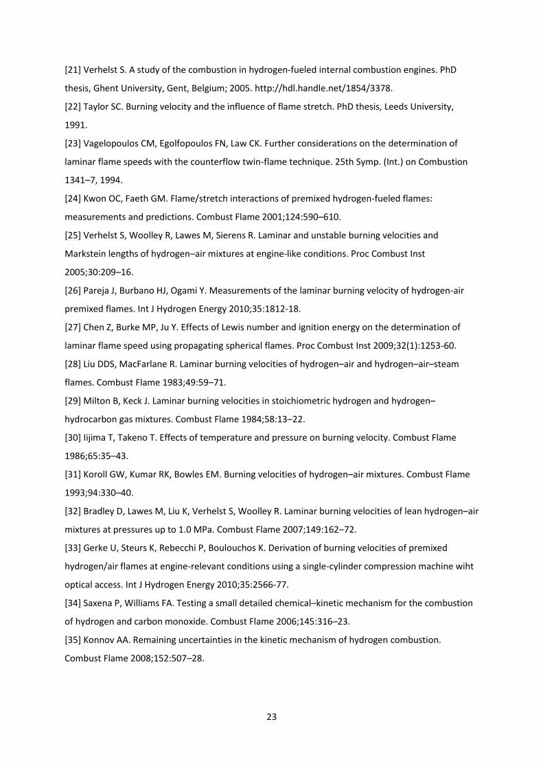
throughout its growth, as illustrated in Fig. 2. The flame speed increases faster than linearly with

decreasing flame stretch rate, consequently the methodology of obtaining stretch-free burning

velocities ul (and its dependence on stretch rate), using eq. (2), is no longer applicable [25,32].

To study the influence of temperature, pressure and residual gas content, Verhelst et al. [21,25]

determined the burning velocity of a spherically expanding flame at a flame radius of 10 mm, for 1 ≤

≤ 3.3, 300 K ≤ T ≤ 430 K, 1 bar ≤ p ≤ 10 bar and 0 % ≤ f ≤ 30 % (with T the temperature, p the

pressure and f the residual gas content, in vol%). This burning velocity is not a fundamental

parameter but, as the authors claim, “is indicative of the burning rate at a fixed, repeatable

condition, representing a compromise that involves a sufficiently large radius to minimize the effects

of the spark ignition, while being small enough to limit the acceleration due to the instabilities”. It is

noteworthy that these are the only data that include the effects of residual gas content, an important

parameter, given the operating strategies that are proposed for H2ICEs.

An alternative methodology has been proposed to obtain ul and Markstein lengths at higher

pressures, from high speed schlieren photography of freely expanding spherical flames. The laminar

burning velocity ul as well as Markstein lengths have been reported for equivalence ratios from =3.3

7

up to stoichiometric, for pressures of 1, 5 and 10 bar [32]. However, this involved numerous

experiments and very high camera frame rates. Furthermore, experimental uncertainty is rather

high, especially on the Markstein lengths.

The most recent attempt at measuring laminar flame speeds with the goal of deriving a correlation

for use in an engine code is reported by Gerke et al. [33]. They extensively discuss the effects of

flame instabilities and demonstrate the resulting complexity of experimentally determining burning

velocities, through measurements of propagating flames in a rapid compression machine. They

measured flame speeds using OH-chemiluminescence as well as deriving flame speeds from the

pressure rise, for a fairly large range of conditions (0.4 ≤ ≤ 2.8, 350 K ≤ T ≤ 700 K, 5 bar ≤ p ≤ 45 bar).

The large variability, large error bars and large deviation between optical (OH) and thermodynamic

(pressure) results clearly illustrate the problems in obtaining hydrogen flame speeds at engine

conditions.

An alternative to the experimental determination is the use of a one-dimensional chemical kinetics

code to calculate ul. The H2/O2 system is one of the simplest reaction mechanisms, it is fairly well

known (with more than 100 mechanisms reported in the literature, e.g., [34]) and computations of ul

are reasonably fast. However, it is perhaps surprising to learn that even for this simple system, there

still exists a number of uncertainties, as recently reviewed by Konnov [35].

4. Literature review of chemical kinetic calculations

As the previous section has demonstrated, experimental determination of laminar burning velocities

is difficult at engine-like conditions because of the occurrence of flame instabilities. Computationally,

flame instabilities can be avoided by the assumption of a one-dimensional, planar flame. With this

assumption, the accuracy of the calculated burning velocities depends on the accuracy of the

molecular transport coefficients, the realism of the chemical kinetic reaction scheme, and the

accuracy of the rate constants.

Several works report results for the laminar burning velocity of hydrogen mixtures calculated with

one-dimensional chemical kinetics. Verhelst et al. report results comparing several published

reaction mechanisms [21,36]. First, based on initial results the reaction mechanism of Ó Conaire et

al. [37] was chosen as it resulted in the best correspondence with the selected experimental data at

atmospheric conditions. Secondly, calculation results were compared with the experimental results

from Verhelst et al. [21,25] for a range of pressures, temperatures, equivalence ratios and residual

gas fractions. Note that these experimental results are not stretch-free burning velocities (see

above). The authors report that the calculations break down for (very) lean mixtures and higher

pressures. For moderately lean to stoichiometric mixtures, the effect of temperature and dilution

8

with residuals is reported to be predicted reasonably well. The inability of steady, planar calculations

to predict burning velocities at very lean mixtures which are in agreement with experimentally

observed values has recently been elucidated by Williams and Grcar [38], who demonstrate both

through asymptotic analysis as through direct numerical simulation, that a premixed flame front can

indeed propagate when the mixture is leaner than the flammability limit for planar flames. They

provide evidence that this is due to the high diffusivity of molecular hydrogen, leading to a

propagation mechanism that can be qualitatively seen as the advancement of a collection of point

sinks of fuel into the fresh mixture. Thus, the high fuel diffusivity leads to a stratification with locally

fuel- enriched zones.

Bradley et al. [32] compare their stretch-free experimentally determined data of ul, at 5 and 10 bar,

to calculations using the reaction mechanisms of Ó Conaire et al. [37] and Konnov [39]. The results

using Konnov's scheme are reported to correspond best to the experimental results within the rather

large uncertainty bands.

CFD simulations have been used by a team from TU Graz and BMW to investigate the mixture

formation and combustion in DI engines [12-14]. The Fluent code was used with the turbulent

burning velocity model by Zimont [40]. The laminar burning velocity was obtained from chemical

kinetic calculations using the reaction scheme of Ó Conaire et al. [37], neglecting the influence of

residual gas. The prediction of the flame propagation and rate of heat release corresponded well

with measurements obtained in an optical engine.

Finally, Gerke et al. [33] also report burning velocity calculations using the scheme of Ó Conaire et al.

[37], and compare them to the experimental results discussed in the previous section. Both their

measured unstable burning velocities as the “stable” burning velocities derived from linear stability

theory are higher than the values computed with the chemical kinetic scheme.

However, as the previous section has shown, experimental stretch-free data are scarce, especially at

engine-like conditions. Thus, one has to keep in mind that validation of reaction mechanisms is very

limited at best. Accurate burning velocity measurements at lean conditions are next to impossible

because of instability. An alternative approach is to test reaction mechanisms on the basis of

measured autoignition times [41,42].

5. Review of published correlations

A number of ul correlations have been used in the literature for hydrogen engine cycle calculations.

Using correlations is mostly preferred to using tabulated ul data as they are more easily implemented

in engine codes. Most correlations use the following form to express the influence of equivalence

9

ratio, pressure, temperature and residual gas content, as originally proposed by Metghalchi and Keck

[43]:

(3)

This form is computationally convenient but assumes the effects of , p, T and f to be independent.

In some cases, the exponents , or are expressed as a function of for a better fit to

experimental data. A correlation of this form was derived for hydrogen mixtures from the

experimental data reported by Verhelst et al. [21,25] and partly validated using an engine code [8].

Knop et al. [11] also proposed a correlation of this form, based largely on the correlation of Verhelst

but extended to <1 (presumably through chemical kinetic calculations but not detailed in the paper)

to allow computations of stratified combustion in DI engines (with locally rich mixtures). The

comparison between simulated and measured engine cycles reported in the paper represents a

limited validation of the correlation. Gerke et al. [33] also use Eq. (3), and present a correlation both

for their measured pressure-derived burning velocities as for the computed burning velocities using a

chemical kinetic mechanism. The effects of equivalence ratio are incorporated both in the ul0 term as

through a dependence of the exponents and . For the residual gas term they refer to Verhelst

[21].

However, Verhelst and Sierens [20] point out that in reality there can be a strong interaction

between the effects of e.g. equivalence ratio and pressure, leading them to propose an alternative

formulation for a laminar burning velocity correlation:

(4)

Here, ul0( ,p), ( ,p), 0( ,p) and 1( ,p) are functions of the form:

(5)

This correlation involves more calculation steps than eq. (3) but is still easily implemented.

D'Errico et al. [9,44] subsequently used this formulation to construct a correlation for the laminar

burning velocity from chemical kinetic calculations using an in-house reaction scheme [45]. The

correlation is claimed to be valid in the range 1 ≤ ≤ 2.8, 500 K ≤ T ≤ 900 K, 1 bar ≤ p ≤ 60 bar. The

validity range for is not stated in the paper. The authors use the correlation in full-cycle

simulations using 1D gas dynamic calculations combined with a quasi-dimensional combustion

model, for a hydrogen engine with cryogenic port injection. Engine cycle simulations were run for

varying engine speed and equivalence ratio and compared to experiments. The combustion pressure

was well predicted for stoichiometric and moderately lean mixtures, but was less satisfactory for

10

(very) lean conditions at medium to high engine speeds. The authors pointed to the effects of

differential diffusion and instabilities for these (very lean) conditions and the high ratios of turbulent

to laminar burning velocities reported for these mixtures [46], which were unaccounted for in the

combustion model.

Although both formulations of a correlation for hydrogen mixtures have been partly validated

through engine simulations, close inspection reveals a problem with the terms describing the effect

of the residual gas fraction:

(6)

The term proposed by Verhelst et al. [21,25] and used in engine cycle simulation [8,11,47] uses a

coefficient that is function of the equivalence ratio:

(7)

Thus, eq. (6) becomes negative for a certain residual gas fraction, depending on equivalence ratio.

For example, for stoichiometric mixtures, a negative is obtained if exceeds 45vol%. However,

hydrogen engine experiments have been reported with external EGR rates of 45% and higher [48,49],

with normal combustion. If such operating strategies are to be simulated, it is clear that the residual

gas terms, eqs. (6) and (7), are inadequate.

The alternative term from eq. (4), proposed by Verhelst et al. [20] and also used in engine cycle

simulation [9,43], uses a coefficient that is function of the equivalence ratio, pressure and

temperature:

(8)

Equation (8) implicates a higher tolerance for dilution with increased temperature ( decreases with

T, thus decreasing the result of eq. (6)). Verhelst et al. [20] gave coefficients for the and

functions (see eq. (5)), valid in the range 1 ≤ ≤ 3, 300 K ≤ T ≤ 800 K, 1 bar ≤ p ≤ 16 bar. For

stoichiometric mixtures the residual gas term also becomes negative if exceeds 45vol%. D’Errico et

al. [9,44] use the same coefficients for the and functions but, as stated above, claim them to be

valid in the range 1 ≤ ≤ 2.8, 500 K ≤ T ≤ 900 K, 1 bar ≤ p ≤ 60 bar. However, such an extrapolation to

much higher pressures leads to non-physical results: depending on the temperature, the residual gas

term can even become greater than 1, implying that diluting the mixture with residual gas would

increase the burning velocity, which clearly is not the case (see also Section 6.4). Also, ref. [9] gives

the same coefficients as ref. [20] although the correlation form for and uses the fuel-to-air

equivalence ratio in [9], as opposed to in ref. [20]. Finally, ref. [9] states that is the mass

fraction of residual gases, whereas it is defined as a volume fraction in ref. [20].

11

In order to allow computation of the laminar burning velocity of hydrogen mixtures at the conditions

that are currently explored in hydrogen engine operating strategies, one-dimensional chemical

kinetic calculations are reported here, the results of which are then fitted to a new correlation form.

6. Calculations and correlation

6.1. Choice of kinetic scheme and range of conditions

Based on the studies discussed in Section 4, the reaction scheme of Konnov [39] was chosen for the

calculation of the laminar burning velocity of hydrogen mixtures, as it is the only scheme (partly)

validated at elevated pressures, using stable burning velocities [32]. The Chem1D one-dimensional

chemical kinetics code developed at the Technical University of Eindhoven [50] was used to calculate

a one-dimensional planar adiabatic flame, the burning velocity of which is by definition.

Calculations have been performed for , , and

. This range covers most of the expected conditions that the unburned

mixture in a hydrogen-fuelled engine will experience. Over 1000 conditions within this range have

been calculated to build up a database to which a correlation can be fitted (see below). The

parameter range is clarified in Table 1.

6.2. Laminar burning velocity without residual gases

In order to determine the correlation the dataset was first examined in more detail to determine the

effect of the different parameters on the laminar burning velocity values. A reference temperature

and pressure were defined (p0 = 1 bar, T0 = 300 K) and used to make the pressure and temperature

non-dimensional. The initial analysis combined with the literature survey suggested the following

functional form for the correlation (Eq. (9)-(10)):

,

0

0

, , , , , , ,

p

l l

Tu p T f u p F p T f

T (9)

0,1,,, ffTpF 0,1,,, ffTpF (10)

This form is based on the earlier correlation of Verhelst and Sierens [20], see Eq. (4), but with a

different correction term F to account for the impact of residual gases. Figure 3 shows the natural

logarithm of ul set out against the natural logarithm of T/T0 for a number of data series without

residual gases. This figure clearly supports the proposed power relationship as all the data series are

almost perfectly linear. This was the case for all considered data points (f = 0). So for each

combination of pressure and equivalence ratio the intercept (ln ul0) and the slope (α) of the linear

12

relation were determined. This resulted in 30 values which were then fit as a function of p/p0 and λ.

As noted by Verhelst and Sierens [20+ both α(λ, p) and ul0(λ, p) are a complex function of p and λ due

to the strong interaction between these variables.

The Levenberg-Marquadt algorithm [51] was used to determine the coefficients of the fitted

equations. This algorithm seeks to reduce the sum of the squared differences (SSD) between the

observed and predicted values. Due to the large spread in ul values (ranging from cm/s to more than

14 m/s) a weighting parameter was used during the fitting, to ensure an accurate fit also for the

lower burning velocities. The weighting was set to the squared reciprocal of the observed value as

this gave the best results (this roughly corresponds to minimizing the relative differences between

observed and predicted values). Each of the proposed equations (see below, Eqs. 11 – 12 – 18) in

this paper is the result of a large number of iterations, whereby different functional forms were fit to

the data. Initially these forms consisted of only linear terms in the different variables (p/p0, λ, f, T/T0).

Progressively terms were added, first ‘pure’ quadratic terms ((p/p0)², λ², f², (T/T0)²) followed by linear

cross terms (e.g. (p/p0) x t, t x f…), inverse linear terms (e.g. 1/(p/p0)) and progressively higher order

terms and combinations of these factors. This was continued until the resulting SSD no longer

decreased. Once this stage was reached it was attempted to ‘trim’ the equation, by selectively

removing terms one by one to see their impact on the SSD. Usually a number of terms could be

removed at this stage, as their impact on the prediction of ul was covered by a cross term. Once such

a relationship was found, the process was repeated but with a different order in which the cross

terms and higher order terms were added to the fit. Eventually the equation which resulted in the

smallest SSD is presented here.

All of the proposed relationships are valid within the entire considered parameter range. Even

though it is possible to reduce the SSD further by splitting the database up into smaller parts (e.g.

lean and rich mixtures), this makes the correlations less generally applicable and presents problems

at the boundaries where they should overlap. It was therefore preferred to present equations which

are valid over the entire range.

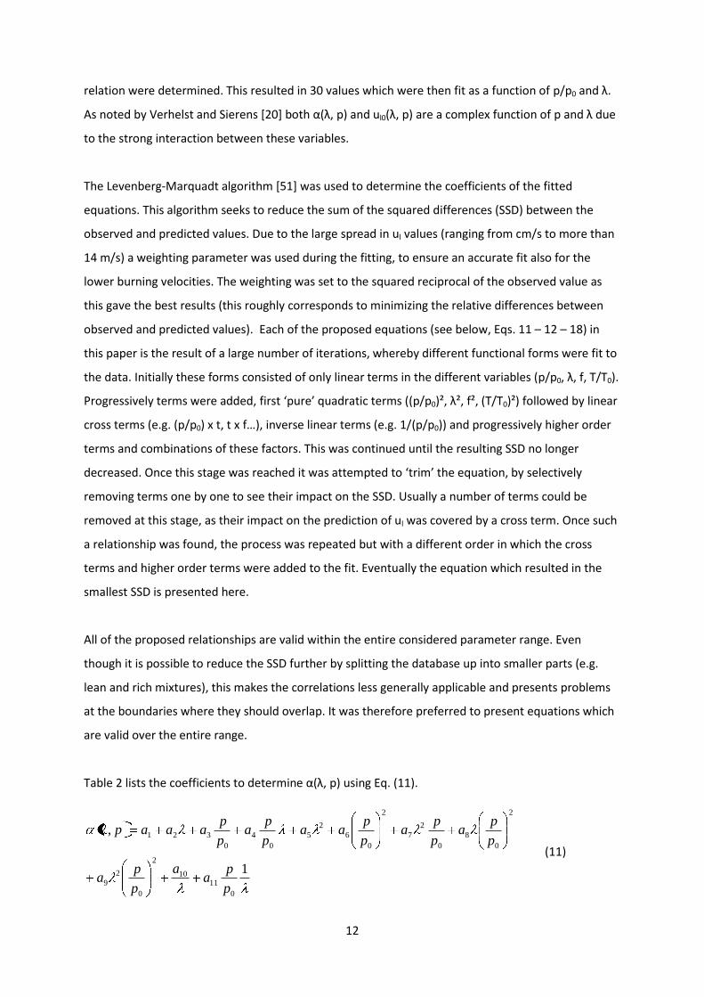
Table 2 lists the coefficients to determine α(λ, p) using Eq. (11).

1

,

0

1110

2

0

2

9

2

0

8

0

2

7

2

0

6

2

5

0

4

0

321

p

pa

a

p

pa

p

pa

p

pa

p

paa

p

pa

p

paaap

(11)

13

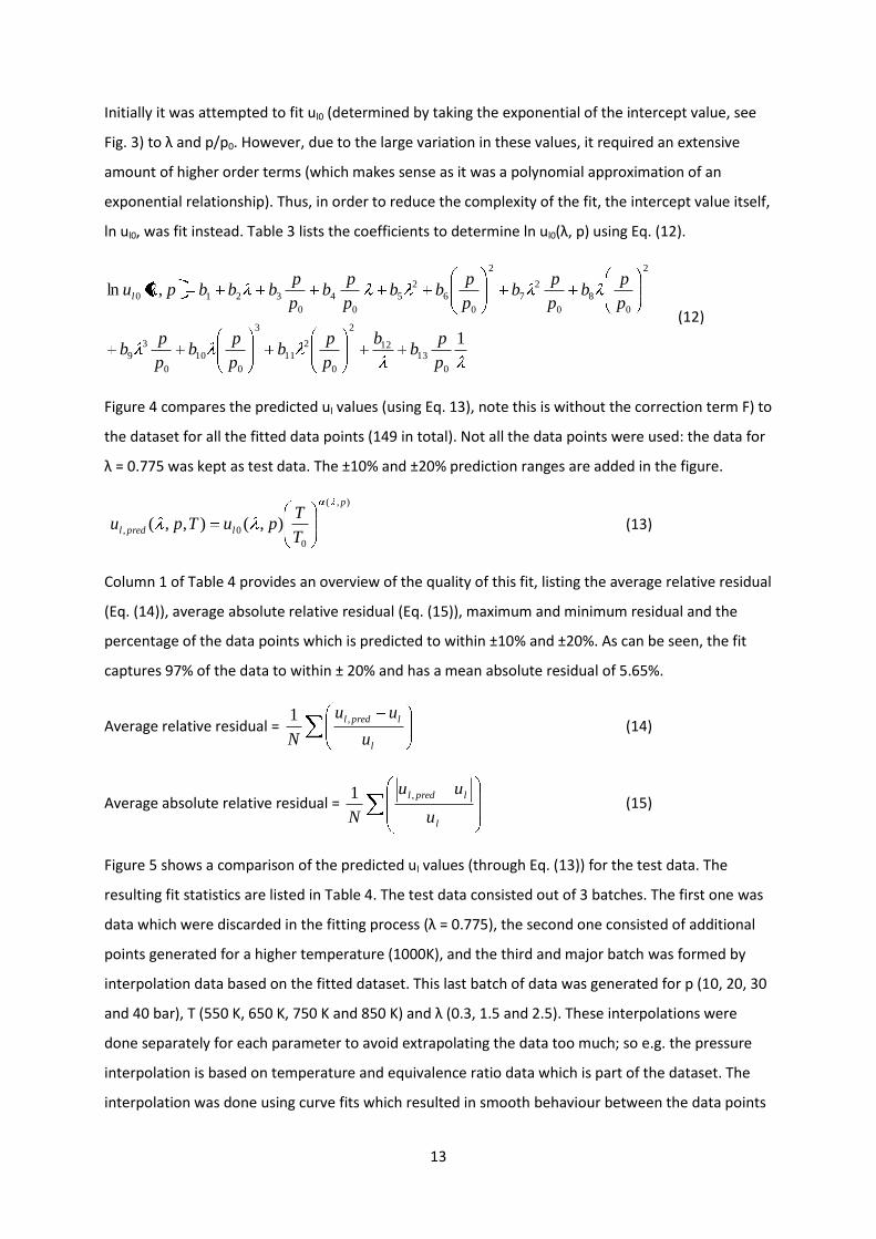
Initially it was attempted to fit ul0 (determined by taking the exponential of the intercept value, see

Fig. 3) to λ and p/p0. However, due to the large variation in these values, it required an extensive

amount of higher order terms (which makes sense as it was a polynomial approximation of an

exponential relationship). Thus, in order to reduce the complexity of the fit, the intercept value itself,

ln ul0, was fit instead. Table 3 lists the coefficients to determine ln ul0(λ, p) using Eq. (12).

1

,ln

0

1312

2

0

2

11

3

0

10

0

3

9

2

0

8

0

2

7

2

0

6

2

5

0

4

0

3210

p

pb

b

p

pb

p

pb

p

pb

p

pb

p

pb

p

pbb

p

pb

p

pbbbpul

(12)

Figure 4 compares the predicted ul values (using Eq. 13), note this is without the correction term F) to

the dataset for all the fitted data points (149 in total). Not all the data points were used: the data for

λ = 0.775 was kept as test data. The ±10% and ±20% prediction ranges are added in the figure.

),(

0

0, ),(),,(

p

lpredlT

TpuTpu (13)

Column 1 of Table 4 provides an overview of the quality of this fit, listing the average relative residual

(Eq. (14)), average absolute relative residual (Eq. (15)), maximum and minimum residual and the

percentage of the data points which is predicted to within ±10% and ±20%. As can be seen, the fit

captures 97% of the data to within ± 20% and has a mean absolute residual of 5.65%.

Average relative residual = l

lpredl

u

uu

N

,1 (14)

Average absolute relative residual = l

lpredl

u

uu

N

,1 (15)

Figure 5 shows a comparison of the predicted ul values (through Eq. (13)) for the test data. The

resulting fit statistics are listed in Table 4. The test data consisted out of 3 batches. The first one was

data which were discarded in the fitting process (λ = 0.775), the second one consisted of additional

points generated for a higher temperature (1000K), and the third and major batch was formed by

interpolation data based on the fitted dataset. This last batch of data was generated for p (10, 20, 30

and 40 bar), T (550 K, 650 K, 750 K and 850 K) and λ (0.3, 1.5 and 2.5). These interpolations were

done separately for each parameter to avoid extrapolating the data too much; so e.g. the pressure

interpolation is based on temperature and equivalence ratio data which is part of the dataset. The

interpolation was done using curve fits which resulted in smooth behaviour between the data points

14

(this was visually verified). Different curves were used, selected after being tested to ensure the

same curve can be used for the entire parameter range. For the temperature fit an exponential curve

was used (Eq. (16)).

bT

fitfitl aeyfTpu 0, ,,, (16)

For the pressure a linear-exponential combination (Eq. (17)) was used.

p

dcpaeyfTpu bp

fitfitl 0, ,,, (17)

For the equivalence ratio a more elaborate fit was needed, whereby first α and ln(u0) were fit using

the exponential linear relationship. These values were then used to compute the test data. Some

examples are shown in Fig. 6 for the temperature (A) and pressure (B), with the filled symbols

corresponding to database values and open symbols to generated test values. This resulted in a

database of 425 test points. Figure 5 compares the predicted ul values (through Eq. (13)) to the test

data. The proposed relationship captures 99% of the test data to within ± 20% and has a mean

absolute residual of 4.78 %. Note how the correlation spans a very large range (from a few cm/s up

to 25 m/s) but is able to provide satisfactory accuracy over the entire range.

6.3. Correction term to account for residual gases

Having first fit the laminar burning velocity for the cases with no residual gases, the correction term

describing the influence and interaction of the pressure, temperature, equivalence ratio and the

volume fraction of the residual gases on the ul values now has to be determined. Verhelst and

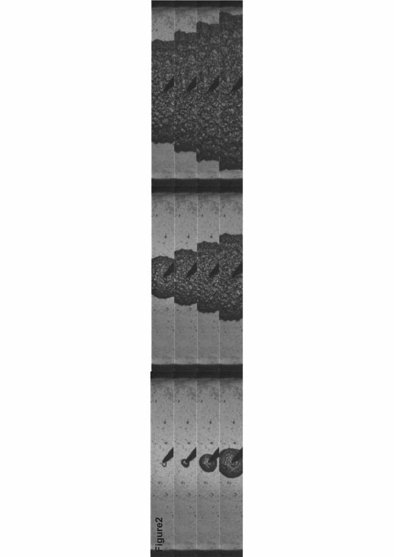
Sierens [20] previously suggested a linear relationship in T and f combined with quadratic terms in p

and λ. For low pressure and equivalence ratio, the trend in T/T0 is indeed linear, but as pressure or

equivalence ratio increases, the trend becomes quadratic. This is indicated in Fig. 7. This figure shows

a number of data series for the correction term (computed as the ratio of the dataset values, with

residuals, to the corresponding predicted values, without residuals, using the correlation proposed

above, Eqs. (11)-(13)) set out against temperature, for stoichiometric mixtures ( =1). Just as for the

data without residual gases a strong coupling between p and λ was found in the correction term,

including higher order terms. Of the different parameters, f has the strongest impact on the value of

the correction term: increasing the residual gas content from 0 to 50 vol % results in a decrease of F

from 1 to about 0. Instead of percentage values (e.g. 20%), decimal values (0.2) are used in all

computations.

15

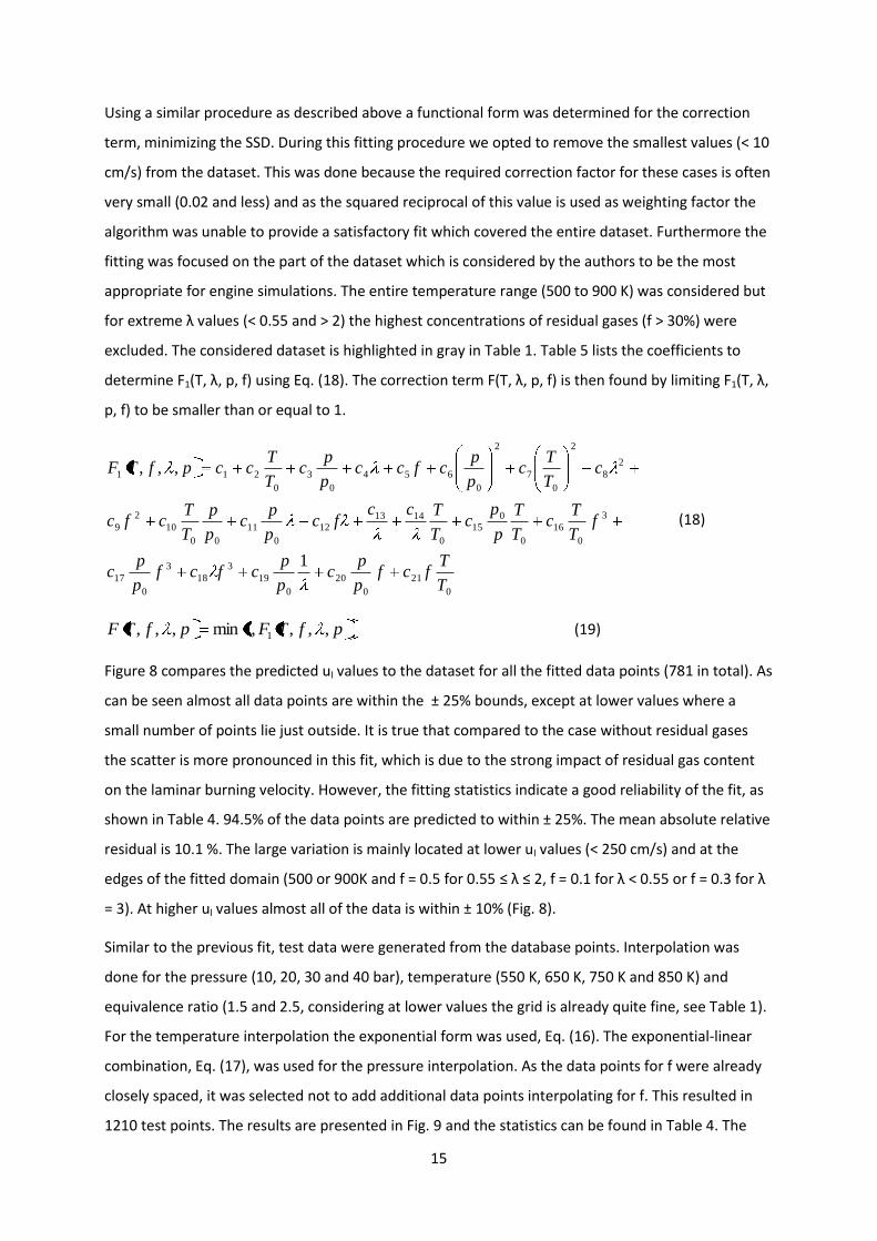
Using a similar procedure as described above a functional form was determined for the correction

term, minimizing the SSD. During this fitting procedure we opted to remove the smallest values (< 10

cm/s) from the dataset. This was done because the required correction factor for these cases is often

very small (0.02 and less) and as the squared reciprocal of this value is used as weighting factor the

algorithm was unable to provide a satisfactory fit which covered the entire dataset. Furthermore the

fitting was focused on the part of the dataset which is considered by the authors to be the most

appropriate for engine simulations. The entire temperature range (500 to 900 K) was considered but

for extreme λ values (< 0.55 and > 2) the highest concentrations of residual gases (f > 30%) were

excluded. The considered dataset is highlighted in gray in Table 1. Table 5 lists the coefficients to

determine F1(T, λ, p, f) using Eq. (18). The correction term F(T, λ, p, f) is then found by limiting F1(T, λ,

p, f) to be smaller than or equal to 1.

0

21

0

20

0

19

3

18

3

0

17

3

0

16

0

0

15

0

1413

12

0

11

00

10

2

9

2

8

2

0

7

2

0

654

0

3

0

211

1

,,,

T

Tfcf

p

pc

p

pcfcf

p

pc

fT

Tc

T

T

p

pc

T

Tccfc

p

pc

p

p

T

Tcfc

cT

Tc

p

pcfcc

p

pc

T

TccpfTF

(18)

pfTFpfTF ,,,,1min,,, 1 (19)

Figure 8 compares the predicted ul values to the dataset for all the fitted data points (781 in total). As

can be seen almost all data points are within the ± 25% bounds, except at lower values where a

small number of points lie just outside. It is true that compared to the case without residual gases

the scatter is more pronounced in this fit, which is due to the strong impact of residual gas content

on the laminar burning velocity. However, the fitting statistics indicate a good reliability of the fit, as

shown in Table 4. 94.5% of the data points are predicted to within ± 25%. The mean absolute relative

residual is 10.1 %. The large variation is mainly located at lower ul values (< 250 cm/s) and at the

edges of the fitted domain (500 or 900K and f = 0.5 for 0.55 ≤ λ ≤ 2, f = 0.1 for λ < 0.55 or f = 0.3 for λ

= 3). At higher ul values almost all of the data is within ± 10% (Fig. 8).

Similar to the previous fit, test data were generated from the database points. Interpolation was

done for the pressure (10, 20, 30 and 40 bar), temperature (550 K, 650 K, 750 K and 850 K) and

equivalence ratio (1.5 and 2.5, considering at lower values the grid is already quite fine, see Table 1).

For the temperature interpolation the exponential form was used, Eq. (16). The exponential-linear

combination, Eq. (17), was used for the pressure interpolation. As the data points for f were already

closely spaced, it was selected not to add additional data points interpolating for f. This resulted in

1210 test points. The results are presented in Fig. 9 and the statistics can be found in Table 4. The

16

proposed relationship is able to predict 94% of the test data to within ± 25% and has a mean

absolute relative residual of 9.3%. The same remarks apply here as for the earlier presented fitted

data (Fig. 8), highlighting the overall quality of the fit, being able to well reproduce the high values

(within ± 10%), and with the scatter mainly located at lower ul values and towards the edges of the

fitted domain.

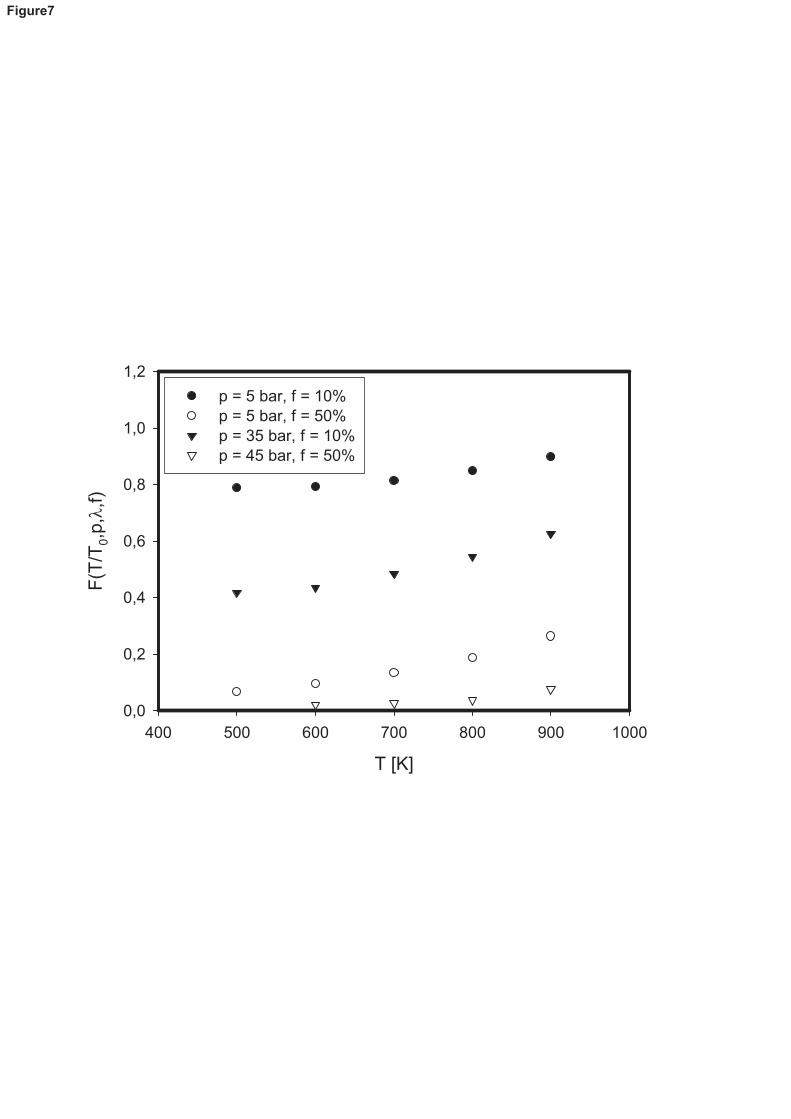
Having determined the coefficients for the correction term F, the full correlation is now known. It

consists of Eq. (9) whereby α(λ,p), ul0(λ,p) and F(T, λ, p, f) are computed through Eqs. (11) – (12) –

(18) – (19) respectively, making use of the coefficients listed in Tables 2, 3 and 5, with p0 and T0 as

given above, f the volume fraction of residuals and ul given in cm/s. Figure 10 presents the

comparison of the predicted values to the database for all available points. The correlation predicts

96.2% of the database points within ±20% and has a mean absolute relative residual of 9.5%.

7. Comparison to other correlations

7.1. Statistical comparison

The correlation presented in the previous section was compared to the correlations published

previously. The comparison includes:

the present correlation, Eq. (9), making use of Eqs. (11) – (12) – (18) – (19)

the correlation presented by Verhelst et al. [21,25] based on experimental data (not

corrected for the effects of stretch and instabilities) , using the correlation form of Eq. (3),

“Verhelst”,

the correlation presented by Knop et al. [11], based on a combination of the correlation by

Verhelst et al. and chemical kinetic calculations, using the correlation form of Eq. (3), “IFP”,

the correlation presented by Gerke et al. [33], based on experimental data (not corrected for

the effects of stretch and instabilities), using the correlation form of Eq. (3), “ETH exp”,

the correlation presented by Gerke et al. [33], based on chemical kinetic calculations using

the mechanism of Ó Conaire et al. [37] , using the correlation form of Eq. (3), “ETH kin. corr.”,

the correlation presented by D’Errico et al. [9], based on chemical kinetic calculations using

the mechanism of Frassoldati et al. [45] , using the correlation form of Eq. (4), “Milano”.

As a basis for the comparison the results from the detailed kinetics calculations were used, because

of the lack of experimental data as discussed earlier. It should be stressed that, as also treated above,

the range of conditions calculated is out of the range of the proven reliability of chemical kinetic

schemes. The calculations were limited to λ≥1 in the case of the correlations of Verhelst et al. and

D’Errico et al., and limited to λ<3 in the case of the two correlations of Gerke et al. and the

correlation of D’Errico et al., to take the reported validity ranges into account.

17

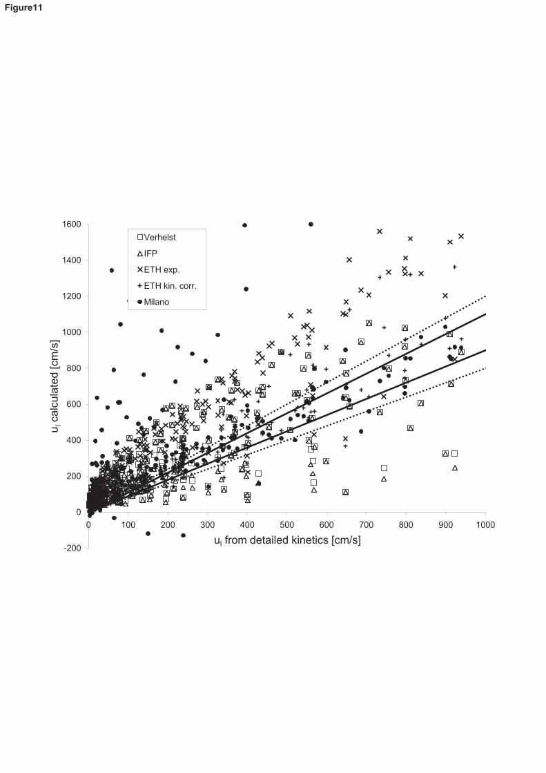
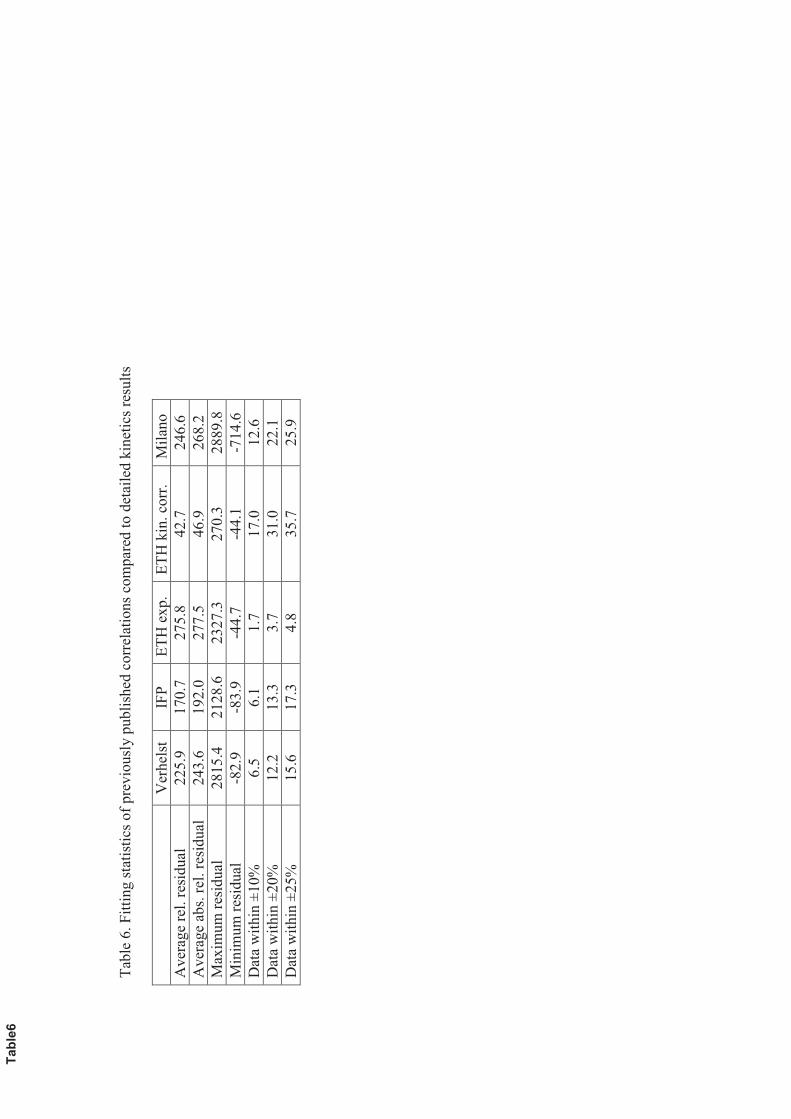
First, a statistical analysis was made, analogous to the analysis that led to Table 4 using Eqs. (14) and

(15). Table 6 lists the average relative residual (Eq. (14)), average absolute relative residual (Eq. (15)),

maximum and minimum residual and the percentage of the results calculated using the different

correlations which correspond to the detailed kinetics results to within ±10%, ±20% and ±25%. Figure

11 plots the burning velocities computed from the different correlations versus the burning velocities

calculated with the one-dimensional chemical kinetics code, showing the ±10% and ±20% ranges.

It is clear from Table 6 and Fig. 11 that there are very large differences, between the results obtained

from the previous correlations and from the present one, and between the previous correlations

themselves. The correlation with the best correspondence to the kinetic results is “ETH kin. corr.”,

which is no surprise being itself a fit to detailed kinetics results within a similar range of conditions.

However, “best correspondence” is a relative notion: looking at the statistics in Table 6 and

confirmed visually from Fig. 11, the differences with the detailed kinetic results presented in this

paper are substantial. This is even more the case for the “Verhelst” and “IFP” correlations, which can

be seen to result in relatively similar values. Looking at the “ETH exp.” correlation results, it is clear

that they are consistently higher than the reference. Finally, using the “Milano” correlation leads to a

wide spread in burning velocities, with some of them even negative. In the following paragraphs, the

differences between the correlations are illustrated for a few selected conditions.

7.2. Graphical illustration

To provide a graphical illustration of the differences in behavior of the correlation presented here

and in previous literature, 5 conditions were selected to compare the present correlation to

previously reported correlations, first for cases without residual gases. As in engines, higher

pressures will be accompanied by higher temperatures, the following conditions were selected from

the database given in Table 1 (marked by the bold X’s):

(5 bar; 500 K)

(15 bar; 600 K)

(25 bar; 700 K)

(35 bar; 800 K)

(45 bar; 900 K)

A more conventional approach would be to illustrate the differences with graphs in which one

parameter is varied while the others are kept constant, but in our opinion this has little practical

relevance as that does not correspond to actual combinations of e.g. p and T. Thus, burning velocities

were calculated for these, admittedly rather arbitrarily chosen, 5 conditions, at three equivalence

ratios, also selected from the database: a rich condition ( =0.55), a stoichiometric mixture ( =1) and

18

a lean one ( =2). The residual gas content was set to be zero for all cases (the correction term for

residuals will be evaluated in the following section).

Figure 12 plots laminar burning velocities for the 5 conditions at the 3 equivalence ratios, calculated

using the correlations listed above. The correlation presented in this paper is marked in the figure as

“Eq. (13)”, as the comparison is limited here to conditions without residuals. The values from the

present database as calculated by Chem1D using Konnov’s mechanism *39] are also shown. Although

5 discrete sets of conditions of pressure and temperature were selected for the comparison, the

results from the correlations are shown using interconnected lines. This was done for clarity. The top

graph of Fig. 12 ( =0.55) does not show results for the correlations “Verhelst” and “Milano”, as these

correlations are only valid for ≥1. In terms of pressure and temperature, the correlation “ETH exp”

is used outside of its validity domain for some points (T>700 K).

As discussed in Section 3, there unfortunately is little or no accurate data for the laminar burning

velocity of hydrogen mixtures at engine conditions, so Fig. 12 does not include experimentally

measured data points. Thus, the correlations can only be compared qualitatively and judged by the

trends they predict. Even so, some interesting observations can be made:

First, the correlation based on cellular flames in a rapid compression machine (“ETH exp”)

predicts substantially higher velocities than all others.

The correlation based on chemical kinetic calculations given by Gerke et al. (“ETH kin. Corr.”)

predicts the burning velocity at 15 bar and 600K to be the lowest of the 5 conditions, for the

3 equivalence ratios. For the other correlations, the lowest burning velocity is for the lowest

temperature condition (5 bar, 500 K) at the rich and stoichiometric conditions. The

correlation based on experimental results given by Gerke et al. (“ETH exp”) also shows a

“discontinuous” trace around the 15 bar, 600 K point, not seen with the other correlations.

The results from the correlations fitted to chemical kinetic calculations using the mechanisms

of Ó Conaire et al. and Konnov, “ETH kin. corr.” and “Eq. (13)” respectively, are fairly close for

the higher pressure and temperature points, especially for the lean case.

At stoichiometry, the results using the correlations “Verhelst” and “IFP” are almost identical

(the lines overlap in the figure), whereas a clear difference can be seen for the lean case.

For the lean case, the correlation proposed by D’Errico et al. (“Milano”) results in a

completely different trend compared to the other correlations.

Finally, it can be seen again that Eq. (13) gives results very close to the detailed results from

the chemical kinetic calculations.

Based on these observations, and although not corroborated by experimental “evidence”, it is safe to

say that the correlations of D’Errico et al. (“Milano”) and Gerke et al. (“ETH kin. corr.”) seem to have

19

a smaller validity range than that claimed by these authors, probably due to the inadequate

correlation form, being too simple to reproduce all the trends given by the detailed kinetic

calculations.

Next, an assessment is made of the behavior of the correction term accounting for the effect of

residual gases.

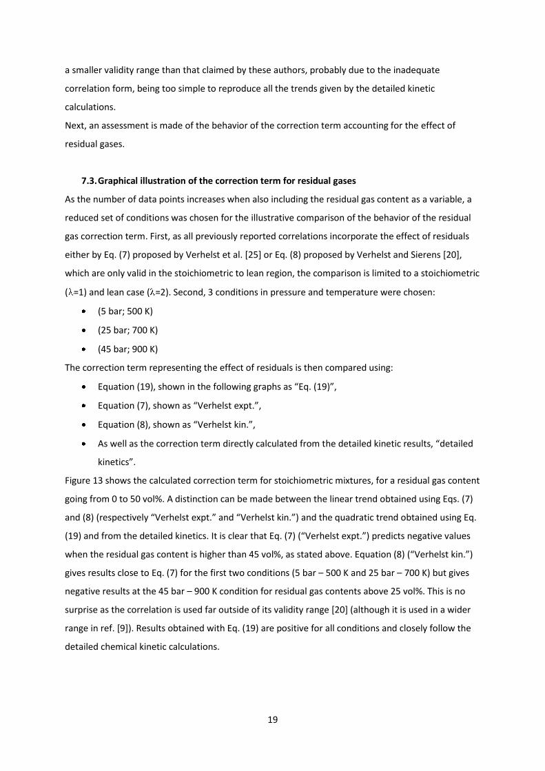
7.3. Graphical illustration of the correction term for residual gases

As the number of data points increases when also including the residual gas content as a variable, a

reduced set of conditions was chosen for the illustrative comparison of the behavior of the residual

gas correction term. First, as all previously reported correlations incorporate the effect of residuals

either by Eq. (7) proposed by Verhelst et al. [25] or Eq. (8) proposed by Verhelst and Sierens [20],

which are only valid in the stoichiometric to lean region, the comparison is limited to a stoichiometric

( =1) and lean case ( =2). Second, 3 conditions in pressure and temperature were chosen:

(5 bar; 500 K)

(25 bar; 700 K)

(45 bar; 900 K)

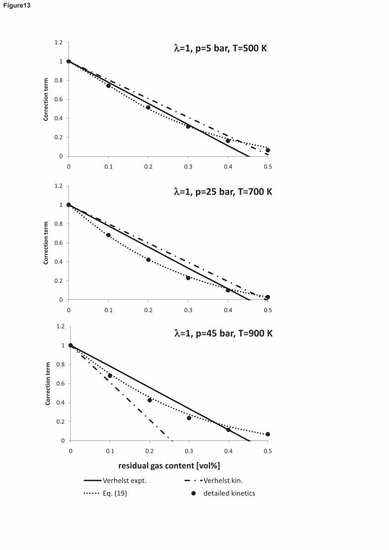
The correction term representing the effect of residuals is then compared using:

Equation (19), shown in the following graphs as “Eq. (19)”,

Equation (7), shown as “Verhelst expt.”,

Equation (8), shown as “Verhelst kin.”,

As well as the correction term directly calculated from the detailed kinetic results, “detailed

kinetics”.

Figure 13 shows the calculated correction term for stoichiometric mixtures, for a residual gas content

going from 0 to 50 vol%. A distinction can be made between the linear trend obtained using Eqs. (7)

and (8) (respectively “Verhelst expt.” and “Verhelst kin.”) and the quadratic trend obtained using Eq.

(19) and from the detailed kinetics. It is clear that Eq. (7) (“Verhelst expt.”) predicts negative values

when the residual gas content is higher than 45 vol%, as stated above. Equation (8) (“Verhelst kin.”)

gives results close to Eq. (7) for the first two conditions (5 bar – 500 K and 25 bar – 700 K) but gives

negative results at the 45 bar – 900 K condition for residual gas contents above 25 vol%. This is no

surprise as the correlation is used far outside of its validity range [20] (although it is used in a wider

range in ref. [9]). Results obtained with Eq. (19) are positive for all conditions and closely follow the

detailed chemical kinetic calculations.

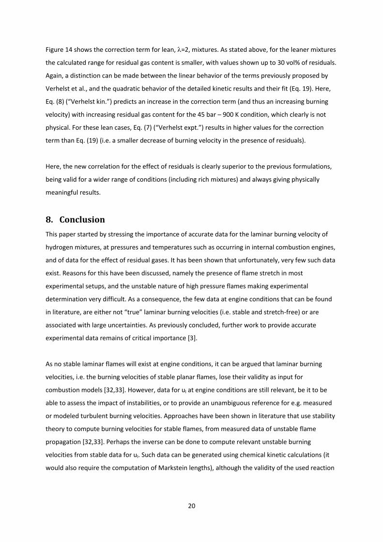
20

Figure 14 shows the correction term for lean, =2, mixtures. As stated above, for the leaner mixtures

the calculated range for residual gas content is smaller, with values shown up to 30 vol% of residuals.

Again, a distinction can be made between the linear behavior of the terms previously proposed by

Verhelst et al., and the quadratic behavior of the detailed kinetic results and their fit (Eq. 19). Here,

Eq. (8) (“Verhelst kin.”) predicts an increase in the correction term (and thus an increasing burning

velocity) with increasing residual gas content for the 45 bar – 900 K condition, which clearly is not

physical. For these lean cases, Eq. (7) (“Verhelst expt.”) results in higher values for the correction

term than Eq. (19) (i.e. a smaller decrease of burning velocity in the presence of residuals).

Here, the new correlation for the effect of residuals is clearly superior to the previous formulations,

being valid for a wider range of conditions (including rich mixtures) and always giving physically

meaningful results.

8. Conclusion

This paper started by stressing the importance of accurate data for the laminar burning velocity of

hydrogen mixtures, at pressures and temperatures such as occurring in internal combustion engines,

and of data for the effect of residual gases. It has been shown that unfortunately, very few such data

exist. Reasons for this have been discussed, namely the presence of flame stretch in most

experimental setups, and the unstable nature of high pressure flames making experimental

determination very difficult. As a consequence, the few data at engine conditions that can be found

in literature, are either not “true” laminar burning velocities (i.e. stable and stretch-free) or are

associated with large uncertainties. As previously concluded, further work to provide accurate

experimental data remains of critical importance [3].

As no stable laminar flames will exist at engine conditions, it can be argued that laminar burning

velocities, i.e. the burning velocities of stable planar flames, lose their validity as input for

combustion models [32,33]. However, data for ul at engine conditions are still relevant, be it to be

able to assess the impact of instabilities, or to provide an unambiguous reference for e.g. measured

or modeled turbulent burning velocities. Approaches have been shown in literature that use stability

theory to compute burning velocities for stable flames, from measured data of unstable flame

propagation [32,33]. Perhaps the inverse can be done to compute relevant unstable burning

velocities from stable data for ul. Such data can be generated using chemical kinetic calculations (it

would also require the computation of Markstein lengths), although the validity of the used reaction

21

scheme is hard to assess precisely because of the lack of experimental data to validate to the

scheme.

Thus, the present paper reports values for the laminar burning velocity of hydrogen mixtures,

obtained from chemical kinetic calculations, using a reaction scheme that was at least partially

validated against burning velocity measurements at increased temperature and pressure. This was

done for a wide range of conditions representative of engine combustion: 0.2 ≤ ≤ 3.0, 500 K ≤ T ≤

900 K, 5 bar ≤ p ≤ 45 bar and 0 vol% ≤ f ≤ 50 vol%. A lot of attention was devoted to a suitable

formulation of a correlation fitting these results, as such a correlation is more easily implemented in

an engine code and allows a better comparison to existing correlations. Deficiencies of the

correlations previously used in literature have been discussed, and a comprehensive study of the

impact of the different parameters resulted in a new type of correlation closely fitting the detailed

kinetic results. As the influence of residual gases was incorporated in a separate correction term, this

can easily be added to other correlations.

Acknowledgements

The authors would like to thank Ronny Tuybens for contributing to this work during his MSc thesis,

and the Combustion Technology section at the Technical University of Eindhoven, in particular Prof.

Philip de Goey, Dr. Bart Somers and Dr. Jeroen Van Oijen, for the use of and help with the Chem1D

code. J. Vancoillie acknowledges the Research Foundation - Flanders (FWO) for the PhD grant

09/ASP/030, J. Demuynck acknowledges the Institute for the Promotion of Innovation

through Science and Technology in Flanders (IWT Vlaanderen) for the PhD grant SB-081139.

References

[1] Abbott D. Hydrogen Without Tears: Addressing the Global Energy Crisis via a Solar to Hydrogen

Pathway, Proc. IEEE 2009;97:1931-4.

[2] Abbott D. Keeping the Energy Debate Clean: How Do We Supply the World’s Energy Needs?, Proc.

IEEE 2010;98:42-66.

[3] Verhelst S, Wallner T, Hydrogen-Fueled Internal Combustion Engines, Progress in Energy and

Combustion Science 2009;35:490-527.

[4] Verhelst S, Maesschalck P, Rombaut N, Sierens R. Efficiency comparison between hydrogen and

gasoline, on a bi-fuel hydrogen/gasoline engine, Int J Hydrogen Energy 2009;34:2504-10.

22

[5] Verhelst S, Maesschalck P, Rombaut N, Sierens R. Increasing the power output of hydrogen

internal combustion engines by means of supercharging and exhaust gas recirculation, Int J Hydrogen

Energy 2009;34:4406–12.

[6] Verhelst S, Verstraeten S, Sierens R. A critical review of experimental research on hydrogen fueled

SI engines. SAE technical paper nr 2006-01-0430. Also in SAE Trans 2006 J Engines 264–74.

[7] White CM, Steeper R, Lutz AE. The hydrogen-fueled internal combustion engine: a technical

review. Int J Hydrogen Energy 2006;31:1292–305.

[8] Verhelst S, Sierens R. A quasi-dimensional model for the power cycle of a hydrogen fuelled ICE. Int

J Hydrogen Energy 2007;32:3545–54.

[9] D’Errico G, Onorati A, Ellgas S. 1d Thermo-fluid dynamic modelling of an SI

single-cylinder H2 engine with cryogenic port injection. Int J Hydrogen Energy 2008;33:5829–41.

[10] Safari H, Jazayeri S, Ebrahimi R. Potentials of NOx emission reduction methods in SI hydrogen

engines: simulation study. Int J Hydrogen Energy 2009;34:1015–25.

[11] Knop V, Benkenida A, Jay S, Colin O. Modelling of combustion and nitrogen oxide formation in

hydrogen-fuelled internal combustion engines within a 3D CFD code. Int J Hydrogen Energy

2008;33:5083–97.

[12] Wimmer A, Wallner T, Ringler J, Gerbig F. H2-direct injection – a highly promising combustion

concept. SAE Paper No. 2005-01-0108 (2005).

[13] Messner D, Wimmer A, Gerke U, Gerbig F. Application and validation of the 3D CFD method for a

hydrogen fueled IC engine with internal mixture formation. SAE Paper No. 2006-01-0448 (2006).

[14] Gerke U, Boulouchos K, Wimmer A. Numerical analysis of the mixture formation and combustion

process in a direct injected hydrogen internal combustion engine. Proceedings 1st international

symposium on hydrogen internal combustion engines. pp. 94–106 (Graz, Austria, 2006).

[15] Clavin P. Dynamic behaviour of premixed flame fronts in laminar and turbulent flows. Prog

Energy Combust Sci 1985;11:1–59.

[16] Williams FA. Combustion theory. 2nd ed. Addison-Wesley; 1985.

[17] Kwon S, Tseng LK, Faeth GM. Laminar burning velocities and transition to unstable flames in

H2/O2/N2 and C3H8/O2/N2 mixtures. Combust Flame 1992;90:230–46.

[18] Hertzberg M. Selective diffusional demixing: occurrence and size of cellular flames. Prog Energy

Combust Sci 1989;15:203–39.

[19] Ilbas M, Crayford AP, Yilmaz I, Bowen PJ, Syred N. Laminar-burning velocities of hydrogen-air and

hydrogen-methane-air mixtures: an experimental study. Int J Hydrogen Energy 2006;31:1768-1779.

[20] Verhelst S, Sierens R. A laminar burning velocity correlation for hydrogen/air mixtures valid at

spark-ignition engine conditions, ASME Spring Engine Technology Conference paper nr. ICES2003-555

(Salzburg, Austria, 2003).

23

[21] Verhelst S. A study of the combustion in hydrogen-fueled internal combustion engines. PhD

thesis, Ghent University, Gent, Belgium; 2005. http://hdl.handle.net/1854/3378.

[22] Taylor SC. Burning velocity and the influence of flame stretch. PhD thesis, Leeds University,

1991.

[23] Vagelopoulos CM, Egolfopoulos FN, Law CK. Further considerations on the determination of

laminar flame speeds with the counterflow twin-flame technique. 25th Symp. (Int.) on Combustion

1341–7, 1994.

[24] Kwon OC, Faeth GM. Flame/stretch interactions of premixed hydrogen-fueled flames:

measurements and predictions. Combust Flame 2001;124:590–610.

[25] Verhelst S, Woolley R, Lawes M, Sierens R. Laminar and unstable burning velocities and

Markstein lengths of hydrogen–air mixtures at engine-like conditions. Proc Combust Inst

2005;30:209–16.

[26] Pareja J, Burbano HJ, Ogami Y. Measurements of the laminar burning velocity of hydrogen-air

premixed flames. Int J Hydrogen Energy 2010;35:1812-18.

[27] Chen Z, Burke MP, Ju Y. Effects of Lewis number and ignition energy on the determination of

laminar flame speed using propagating spherical flames. Proc Combust Inst 2009;32(1):1253-60.

[28] Liu DDS, MacFarlane R. Laminar burning velocities of hydrogen–air and hydrogen–air–steam

flames. Combust Flame 1983;49:59–71.

[29] Milton B, Keck J. Laminar burning velocities in stoichiometric hydrogen and hydrogen–

hydrocarbon gas mixtures. Combust Flame 1984;58:13–22.

[30] Iijima T, Takeno T. Effects of temperature and pressure on burning velocity. Combust Flame

1986;65:35–43.

[31] Koroll GW, Kumar RK, Bowles EM. Burning velocities of hydrogen–air mixtures. Combust Flame

1993;94:330–40.

[32] Bradley D, Lawes M, Liu K, Verhelst S, Woolley R. Laminar burning velocities of lean hydrogen–air

mixtures at pressures up to 1.0 MPa. Combust Flame 2007;149:162–72.

[33] Gerke U, Steurs K, Rebecchi P, Boulouchos K. Derivation of burning velocities of premixed

hydrogen/air flames at engine-relevant conditions using a single-cylinder compression machine wiht

optical access. Int J Hydrogen Energy 2010;35:2566-77.

[34] Saxena P, Williams FA. Testing a small detailed chemical–kinetic mechanism for the combustion

of hydrogen and carbon monoxide. Combust Flame 2006;145:316–23.

[35] Konnov AA. Remaining uncertainties in the kinetic mechanism of hydrogen combustion.

Combust Flame 2008;152:507–28.

24

[36] Verhelst S, Sierens R. A Two-Zone Thermodynamic Model for Hydrogen-Fueled S.I. Engines, 7th

COMODIA – Int. Conf. on Modeling and Diagnostics for Advanced Engine Systems, Sapporo, Japan,

July 28-31 2008, paper FL1-3

[37] Ó Conaire M, Curran H, Simmie J, Pitz W, Westbrook C. A comprehensive modeling study of

hydrogen oxidation. Int J Chem Kinet 2004;36:603–22.

[38] Williams FA, Grcar JF. A hypothetical burning-velocity formula for very lean hydrogen–air flames.

Proc Combust Inst 2009;32:1351–7.

[39] Konnov AA. Refinement of the kinetic mechanism of hydrogen combustion. J Adv Chem Phys

2004;23:5–18.

[40] Zimont V. Gas premixed combustion at high turbulence. Turbulent flame closure combustion

model. Exp Ther Fluid Sci 2000;21:179–86.

[41] Williams FA. Detailed and reduced chemistry for hydrogen autoignition. J Loss Prev Process

Indust 2008;21:131–5.

[42] Ströhle J, Myhrvold T. An evaluation of detailed reaction mechanisms for hydrogen combustion

under gas turbine conditions. Int J Hydrogen Energy 2007;32:125-135.

[43] Metghalchi M, Keck JC. Laminar Burning Velocity of Propane-Air Mixtures at High Temperature

and Pressure, Combust Flame 1980;38:143-54.

[44] D’Errico G, Onorati A, Ellgas S, Obieglo A. Thermo-fluid dynamic simulation of a S.I. single-

cylinder H2 engine and comparison with experimental data. ASME Spring Engine Technology

Conference paper nr. ICES2006-1311 (Aachen, Germany, 2006).

[45] Frassoldati A, Faravelli T, Ranzi E. A wide range modeling study of NOX formation and nitrogen

chemistry in hydrogen combustion. Int J Hydrogen Energy 2006;31:2310-28.

[46] Lipatnikov A, Chomiak J. Molecular transport effects on turbulent flame propagation and

structure. Prog Energy Combust Sci 2005;31:1–73.

[47] Gerke U. Numerical analysis of mixture formation and combustion in a hydrogen direct-injection

internal combustion engine. PhD thesis, Swiss Federal Institute of Technology, Zurich, Switzerland.

[48] Brewster S, Bleechmore C. Dilution Strategies for Load and NOx Management in a Hydrogen

Fuelled Direct Injection Engine. SAE technical paper nr 2007-01-4097.

[49] Verhelst S, Sierens R. Combustion Studies for PFI Hydrogen IC Engines. SAE technical paper nr

2007-01-3610.

[50] Combustion Technology group, Technical University of Eindhoven,

http://www.combustion.tue.nl.

[51] More JJ. The Levenberg-Marquardt algorithm: implementation and theory. Proceedings of the

1977 Dundee conference on numerical analysis (Berlin, Heidelberg, New York, Tokyo) (G. A. Watson,

ed.), Lecture notes in mathematics 630, Springer Verlag, 1978, pp. 105-116.

25

Figure and table captions

Table captions

Table 1. The database of ul values

Table 2. Coefficients for Eq. (11)

Table 3. Coefficients for Eq. (12)

Table 4. Fitting statistics of Eq. (13) (partial fit, f=0) and Eq. (9)-(18)-(19) (full fit, f≥0) compared to

fitted data and test data

Table 5. Coefficients for Eq. (18)

Table 6. Fitting statistics of previously published correlations compared to detailed kinetics results

Figure captions

Figure 1. Laminar burning velocities plotted against air-to-fuel equivalence ratio, for NTP hydrogen-

air flames. Experimentally derived correlations from Liu and MacFarlane [27], Milton and Keck [28],

Iijima and Takeno [29] and Koroll et al. [30]. Other experimental data from Taylor [21], Vagelopoulos

et al. [22], Kwon and Faeth [23] and Verhelst et al. [24].

Figure 2. Schlieren photographs of a =1.25, 300 K, 5 bar hydrogen-air flame, taken in a constant

volume combustion chamber (time interval 0.385 ms), illustrating the cellular nature of the flame

caused by flame front instability.

Figure 3. Plot of the natural logarithm of ul set out against the natural logarithm of the

dimensionless temperature T/T0. Various data series are shown (pressure p given in bar), spanning

the entire database illustrating the generality of the proposed power relationship.

Figure 4. Comparison between the predicted laminar burning velocity values ul,pred using the

correlation (Eqs. (11)-(13)) and the source data upon which the correlation is based (no residual

gases). The ± 10% (solid lines) and ± 20% (dashed lines) are indicated.

Figure 5. Comparison between the predicted laminar burning velocity values ul,pred using the

correlation (Eqs. (11)-(13)) and the test data (no residual gases). The ± 10% (solid lines) and ± 20%

(dashed lines) are indicated.

Figure 6. Examples of test data (open symbols) generated based on the dataset (black symbols) for

intermediate temperatures (A) and pressures (B). Various data series are shown, spanning the entire

database.

Figure 7. Trend analysis of the correction term F(T, λ, p, f) for varying temperatures and =1.

26

Figure 8. Comparison between the predicted laminar burning velocity values ul,pred using the

correlation (Eqs. (9)-(11)-(13)-(18)-(19)) and the source data upon which the correlation is based

(with residual gases). The ± 10% (solid lines) and ± 25% (dashed lines) are indicated.

Figure 9. Comparison between the predicted laminar burning velocity values ul,pred using the

correlation (Eqs. (9)-(11)-(13)-(18)-(19)) and the test data (with residual gases). The ± 10% (solid

lines) and ± 25% (dashed lines) are indicated.

Figure 10. Comparison between the predicted laminar burning velocity values ul,pred using the

correlation (Eqs. (9)-(11)-(13)-(18)-(19)) and the entire dataset (fitted and test data). The ± 10%

(solid lines) and ± 25% (dashed lines) are indicated.

Figure 11. Comparison between the laminar burning velocity values using previously published

correlations (ul calculated) to the values obtained using the present chemical kinetic computations

(ul from detailed kinetics). The ± 10% (solid lines) and ± 20% (dashed lines) are indicated.

Figure 12. Comparison of the calculated burning velocities for 5 combinations of pressure and

temperature, at 3 air-to-fuel equivalence ratios. Burning velocities calculated with the correlations

of Verhelst et al. [20,24+ (“Verhelst”), Knop et al. [11+ (“IFP”), Gerke et al. *32] (on the basis of their

experimental results – “ETH exp” and of chemical kinetics – “ETH kin. corr.”), D’Errico et al. *7+

(“Milano”), and Eq. (13). Results from the detailed kinetics also shown.

Figure 13. Comparison of the calculated correction term as a function of residual gas content, for 3

combinations of pressure and temperature, for stoichiometric mixtures. Calculations done with the

correlations of Verhelst et al. [19,24+ (respectively “Verhelst kin.” and “Verhelst expt.”) and Eq. (19).

Results from the detailed kinetics also shown.

Figure 14. Comparison of the calculated correction term as a function of residual gas content, for 3

combinations of pressure and temperature, for an air-to-fuel equivalence ratio =2. Calculations

done with the correlations of Verhelst et al. [19,24+ (respectively “Verhelst kin.” and “Verhelst

expt.”) and Eq. (19). Results from the detailed kinetics also shown.

0

0.5

1

1.5

2

2.5

3

3.5

4

0.5 1 1.5 2 2.5 3

ul(m/s

)

l

Liu&MacFarlane

Iijima&Takeno

Koroll et al.

Milton&Keck

Taylor

Kwon&Faeth

Vagelopoulos et al.

Verhelst et al.

Figure1

Figure2

ln(T/T0)

0,4 0,5 0,6 0,7 0,8 0,9 1,0 1,1 1,2

ln u

l

0

1

2

3

4

5

6

7

8

p = 5 bar, = 0.2

p = 5 bar, = 0.55

p = 5 bar, = 1

p = 5 bar, = 2

p = 5 bar, = 3

p = 45 bar, = 0.2

p = 45 bar, = 0.55

p = 45 bar, = 1

p = 45 bar, = 2

p = 45 bar, = 3

Figure3

ul [cm/s]

0 500 1000 1500 2000

ul,p

red [cm

/s]

0

500

1000

1500

2000

Figure4

Figure5

Figure6

T [K]

400 500 600 700 800 900 1000

F(T

/T0,p

, ,f)

0,0

0,2

0,4

0,6

0,8

1,0

1,2

p = 5 bar, f = 10%

p = 5 bar, f = 50%

p = 35 bar, f = 10%

p = 45 bar, f = 50%

Figure7

Figure8

Figure9

Figure10

-200

0

200

400

600

800

1000

1200

1400

1600

0 100 200 300 400 500 600 700 800 900 1000

ulcalc

ula

ted [cm

/s]

ul from detailed kinetics [cm/s]

Verhelst

IFP

ETH exp.

ETH kin. corr.

Milano

Figure11

500

700

900

1100

1300

1500

1700

1900

2100

500 600 700 800 900

ul[c

m/s

]temperature [K]

l=0.55

400

600

800

1000

1200

1400

1600

ul[c

m/s

]

l=1

50

150

250

350

450

550

5 15 25 35 45

ul[c

m/s

]

pressure [bar]

l=2

Eq. (13) Verhelst IFP

ETH exp ETH kin. corr. Milano

detailed kinetics

Figure12

0

0.2

0.4

0.6

0.8

1

1.2

0 0.1 0.2 0.3 0.4 0.5

Co

rre

ctio

n t

erm

l=1, p=5 bar, T=500 K

0

0.2

0.4

0.6

0.8

1

1.2

0 0.1 0.2 0.3 0.4 0.5

Co

rre

ctio

n t

erm

l=1, p=25 bar, T=700 K

0

0.2

0.4

0.6

0.8

1

1.2

0 0.1 0.2 0.3 0.4 0.5

Co

rre

ctio

n t

erm

residual gas content [vol%]

l=1, p=45 bar, T=900 K

Verhelst expt. Verhelst kin.

Eq. (19) detailed kinetics

Figure13

0

0.2

0.4

0.6

0.8

1

1.2

0 0.1 0.2 0.3

Co

rre

ctio

n t

erm

l=2, p=5 bar, T=500 K

0

0.2

0.4

0.6

0.8

1

1.2

0 0.1 0.2 0.3

Co

rre

ctio

n t

erm

l=2, p=25 bar, T=700 K

0

0.2

0.4

0.6

0.8

1

1.2

0 0.1 0.2 0.3

Co

rre

ctio

n t

erm

residual gas content [vol%]

l=2, p=45 bar, T=900 K

Verhelst expt. Verhelst kin.

Eq. (19) detailed kinetics

Figure14

Table 1: The database of ul values

p\T 500 K 600 K 700 K 800 K 900 K λ\f 0 0.1 0.2 0.3 0.4 0.5

5 X X X X X 0.2 X X - - - -

15 X X X X X 0.38 X X X X - -

25 X X X X X 0.55 X X X X X X

35 X X X X X 0.775 X X X X X X

45 X X X X X 1 X X X X X X

2 X X X X X X

3 X X X X X X

Table1

Table 2: coefficients for Eq. (11)

a1 0.584069

a2 1.097884

a3 -3.683272 e-2

a4 2.454259 e-2

a5 0.104381

a6 -4.119350 e-4

a7 7.621143 e-3

a8 7.62759 e-4

a9 -4.498380 e-4

a10 0.331465

a11 2.165434 e-2

Table2

Table 3: coefficients for Eq. (12)

b1 7.505661

b2 -1.903711

b3 5.380840 e-2

b4 -3.936929 e-2

b5 1.896873 e-2

b6 5.964680 e-4

b7 -3.010525 e-2

b8 -3.431092 e-4

b9 9.023031 e-4

b10 -1.556492 e-5

b11 8.452404 e-4

b12 -0.478534

b13 -3.105883 e-2

Table3

Tab

le 4

. F

itti

ng s

tati

stic

s of

Eq. (1

3)

(par

tial

fit

, f=

0)

and E

q. (9

)-(1

8)-

(19)

(full

fit

, f≥

0)

com

par

ed t

o f

itte

d d

ata

and t

est

dat

a

u

l,p

red

(Eq. (1

3))

ul,

pre

d (

Eq. (1

3))

:

test

dat

a

ul,

pre

d

(Eq. (1

3)-

(18)-

(19))

ul,

pre

d (

Eq.

(13)-

(18

)-(1

9))

:

test

dat

a

Aver

age

rel.

res

idual

0.0

07

%

-0.8

1%

-4

.3%

-1

.5%

Aver

age

abs.

rel

. re

sidual

5.6

7%

4.7

8%

10

.1%

9.3

%

Max

imum

res

idual

21.7

%

25.9

%

41

%

48.4

%

Min

imum

res

idual

-2

4%

-2

4.2

%

-44

%

-34.1

%

Dat

a w

ithin

±10%

85.3

%

94.3

%

73.1

%

84%

Dat

a w

ithin

±20%

96.6

%

99.1

%

87.8

%

89%

Dat

a w

ithin

±25%

100%

99.7

%

94.5

%

94%

Table4

Table 5: coefficients for Eq. (18)

c1 1.782191

c2 -1.945813E-01

c3 -4.071734E-03

c4 -4.987061E-01

c5 -4.347767

c6 8.576177E-05

c7 4.490150E-02

c8 7.878902E-02

c9 4.243647

c10 -2.052509E-03

c11 3.724404E-03

c12 -2.114637E-01

c13 -2.224738E-01

c14 4.624703E-02

c15 2.116186E-01

c16 -2.098941

c17 7.029643E-02

c18 1.334951

c19 4.861730E-04

c20 -1.915344E-02

c21 6.146191E-01

Table5

Tab

le 6

. F

itti

ng s

tati

stic

s of

pre

vio

usl

y p

ubli

shed

corr

elat

ions

com

par

ed t

o d

etai

led k

inet

ics

resu

lts

V

erhel

st

IFP

E

TH

ex

p.

ET

H k

in. co

rr.

Mil

ano

Aver

age

rel.

res

idual

225.9

170.7

275.8

42.7

246.6

Aver

age

abs.

rel

. re

sidual

243.6

192.0

277.5

46.9

268.2

Max

imum

res

idual

2815.4

2128.6

2327.3

270.3

2889.8

Min

imum

res

idual

-8

2.9

-8

3.9

-4

4.7

-4

4.1

-7

14.6

Dat

a w

ithin

±10%

6.5

6.1

1.7

17.0

12.6

Dat

a w

ithin

±20%

12.2

13.3

3.7

31.0

22.1

Dat

a w

ithin

±25%

15.6

17.3

4.8

35.7

25.9

Table6