The Unconventional Energy Revolution: Estimated Energy Savings for Public School Districts and State and Local Governments Prepared for: American Petroleum Institute Prepared by: IHS Global Inc. 1150 Connecticut Ave, NW, Suite 401 Washington, D.C. 20036 May 28, 2014
Transcript
The Unconventional Energy Revolution: Estimated Energy Savings for Public School Districts and State and Local
Governments
Prepared for:
American Petroleum Institute
Prepared by:
IHS Global Inc. 1150 Connecticut Ave, NW, Suite 401
Washington, D.C. 20036
May 28, 2014
Savings by State & Local Governments and School Districts from Unconventional Energy Development
Final Report i IHS Global Inc.
CONTACT INFORMATION RICHARD FULLENBAUM Vice President, IHS Economics Consulting IHS Global Inc. 1150 Connecticut Ave., NW, Suite 401 Washington, DC 20036 Tel: 202-481-9212 Email: [email protected] JAMES DIFFLEY Senior Director, IHS Economics Consulting IHS Global Inc. 1650 Arch Street, Suite 2000 Philadelphia, PA 190103 Tel: 215-789-7422 Email: [email protected] PHIL HOPKINS Senior Consultant, IHS Economics Consulting IHS Global Inc. 1650 Arch Street, Suite 2000 Philadelphia, PA 190103 Tel: 215-789-7468 Email: [email protected]
State and local governments considered ...................................................................................................... 2
Reference year ................................................................................................................................................ 3
IHS studies of the unconventional energy sector .......................................................................................... 3
Energy use and spending ..................................................................................................................................... 5
Energy consumption by fuel type .................................................................................................................. 5
Energy intensity .............................................................................................................................................. 7
Energy consumption by end use .................................................................................................................... 8
Regional variations in energy use .................................................................................................................. 8
Public elementary and secondary school districts ...................................................................................... 16
State and local governments ........................................................................................................................ 17
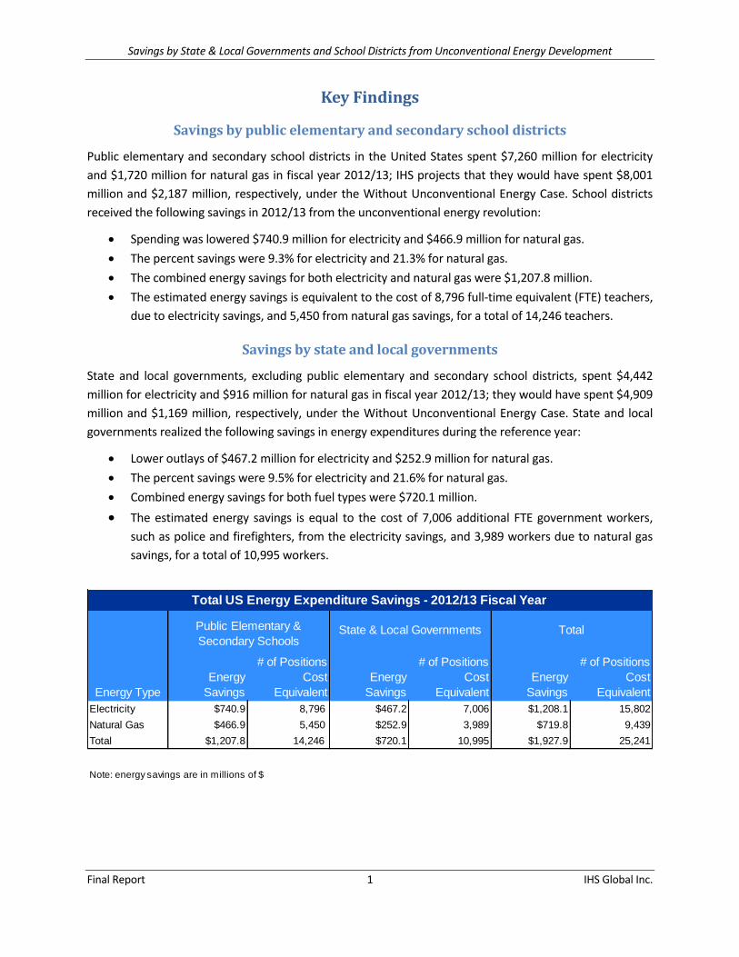
Natural Gas $466.9 5,450 $252.9 3,989 $719.8 9,439
Total $1,207.8 14,246 $720.1 10,995 $1,927.9 25,241
Public Elementary &
Secondary SchoolsState & Local Governments
Note: energy savings are in millions of $
Total
Total US Energy Expenditure Savings - 2012/13 Fiscal Year
Savings by State & Local Governments and School Districts from Unconventional Energy Development
Final Report 2 IHS Global Inc.
Introduction
Purpose
In the recently completed study—America’s New Energy Future (ANEF) – Volume 3: A Manufacturing
Renaissance—IHS estimated the effect of the unconventional energy revolution on the US economy.
This revolution has increased domestic oil and natural gas production, lowered prices for oil and natural
gas, and increased energy investment. These direct industry effects, in turn, have affected the national
economy, including GDP, foreign trade, industrial production, and household disposable income. The
ANEF study determined lower prices for oil and natural gas, the accompanying declines in electricity
prices, and other economic effects, increased US households’ annual disposable income by $1,200 in
2012.
API retained IHS to extend its ANEF results to estimate similar energy savings due to the unconventional
energy revolution received by state and local governments & public elementary and secondary school
districts across the US. These institutions paid lower rates for much of their energy use as a direct result of
the unconventional energy revolution. The savings are the differences between actual spending for energy
by state and local governments & school districts, and estimates of what they would have paid under a
scenario with higher oil and natural gas prices which would have occurred without US unconventional oil
and natural gas development.
State and local governments considered
This study estimates the energy savings received by: 1) state and local governments, excluding public
elementary and secondary school districts, and 2) public elementary and secondary school districts. The
local, non-education, government sector is large and varied, as it includes county, city, and municipal
governments, authorities (e.g., water and sewer systems, solid waste management authorities, and local
public utilities) and special-use districts, such as those for libraries, irrigation, etc. The term “state and local
governments,” as it is used in this report, does not include public elementary and secondary schools
districts.
According the Census Bureau, in 2012, there were 14,178 public school districts in the United States.
Private K-to-12 schools are not considered in the analysis of public elementary and secondary schools, due
to the difficulty in obtaining energy spending data. Charter schools that are public schools are included in
the study. The inability to consider private schools does not significantly affect the results, because,
according to the United States Department of Education, in 2009, about 90% of all students in grades K to
12 attended public schools, so those schools account for the vast majority of energy spending by all K-to-
12 schools.
Savings by State & Local Governments and School Districts from Unconventional Energy Development
Final Report 3 IHS Global Inc.
Reference year
The reference year of analysis for this study is fiscal year (FY) 2012/13, which was from 1 July 2012 to 30
June 2013. It was selected because: 1) virtually all state governments, many local governments, and most
public elementary and secondary districts use a 1 July to 30 June fiscal year; and 2) it was the most recent
fiscal year for which detailed energy spending figures were consistently available. If information could not
be obtained for the reference year, but had been published for prior fiscal years, price indices were used to
convert figures to FY 2012/13 dollars. Quarterly values for price indices were used to convert calendar-
year data to a fiscal-year basis.
Scenarios evaluated
This study estimated energy spending savings by state and local governments, and by public elementary
and secondary school districts, during the reference year for two scenarios:
The Base Case uses energy cost estimates for 2012 and 2013 from the IHS ANEF study, which
includes unconventional oil and natural gas production. This report uses the term “Base Case” to
refer to this scenario.
The Without Unconventional Energy Case is the energy cost environment that would have existed
without unconventional oil and natural gas.
In order to calculate benefits from the unconventional energy revolution, IHS’s energy group provided
estimates of electricity and natural gas prices under both scenarios in FY 2012/13. Because this study
estimates actual energy spending by both types of governments, the appropriate metric is the retail or
delivered price of electricity and natural gas. Finally, we use commercial prices for electricity and natural
gas, as both types of governments are usually classified as commercial customers by electric and natural
gas utilities.
IHS studies of the unconventional energy sector
Our ANEF study estimated that the economic benefit from the unconventional energy revolution was an
increase of $1,200 in annual real disposable income per US household in 2012. These economic benefits
are the cumulative result of higher spending and investment in the unconventional energy value chain, in
addition to lower fuel and feedstock prices paid by the US manufacturing sector, especially by energy-
intensive sub-sectors such as chemicals, oil refining, food, and metals. The $1,200 figure is the total value
of economic benefits across the US economy that households received, including:
Lower consumption costs from reduced prices for natural gas used for heating and water heating.
Reduced prices for electricity due to lower costs for natural gas used as a fuel in electricity
generating plants.
Lower prices for consumer goods and services, especially for energy-intensive products, due to
lower input costs.
Higher wage income as the manufacturing renaissance increases industrial activity, leading to
rising employment and wage levels in manufacturing, and in the downstream sectors that use its
goods as inputs.
Savings by State & Local Governments and School Districts from Unconventional Energy Development
Final Report 4 IHS Global Inc.
IHS forecasts in the ANEF study that the increase in real disposable income per US household provided by
unconventional oil and natural gas revolution will grow over time, from just over $2,000 in 2015, to more
than $3,500 by 2025.1
1 IHS, America’s New Energy Future: The Unconventional Oil and Gas Revolution and the US Economy, Volume 3: A Manufacturing Renaissance, September 2013.
Savings by State & Local Governments and School Districts from Unconventional Energy Development
Final Report 5 IHS Global Inc.
Energy use and spending
This study includes the following types of energy consumed in buildings used by both types of
governments.
Electricity
Natural gas
Fuel oil
Propane
Other (e.g., steam, geothermal, compressed natural gas, etc.)
This study does not include fuel used in vehicles.
IHS conducted a literature review to describe energy use patterns in state and local governments, and in
elementary and secondary school buildings. Understanding energy use patterns by fuel type and end use
category was necessary to evaluate how the differences in retail energy prices between the two scenarios
had affected energy spending by the two types of governments. For example, lower prices for natural gas
have caused both types of governments in the New England and Mid-Atlantic Census divisions to
substitute it for fuel oil in systems used to provide space and water heating. At the same time, in order to
take maximum advantage of lower natural gas wholesale prices, both types of governments are also are
entering into longer-term contracts. While it is outside the scope of this study, both types of governments
are also increasingly considering using natural gas-fueled vehicles in order to lower their transportation
costs. While the retail price of commercial electricity has fallen due to lower natural gas wholesale prices,
it is still high enough to provide both types of governments with an incentive to reduce their electricity
consumption.
Data on energy spending, consumption patterns by fuel type, and end use in government buildings is from
the United States Department of Energy’s (USDOE) Building Energy Data Book. The information contained
in this source is for calendar year 2003, so it should be used knowing that energy use patterns have likely
changed since then, especially following the unconventional energy revolution’s start in the late 2000s.
After talking with energy experts from both USDOE and IHS, we feel the energy consumption patterns by
end use, and to a lesser extent by fuel type, are still generally applicable. It is certain the energy share used
for computers has increased since 2003, as both types of governments have invested more in information
technology (IT). For example, many school districts have increased the number of computers and other
devices in their buildings.
IHS analyzed energy use information in the nine census divisions for elementary and secondary buildings,
and for state and local government buildings, which are defined below in the methodology section.
Energy consumption by fuel type
Energy consumption on a British thermal unit (Btu) basis by fuel type varied significantly in 2003 between
elementary and secondary buildings, and state and local government buildings. Fuel use in school buildings
was almost evenly split between electricity (46.9%) and natural gas (41%) with the remaining fuel types
making up just over 12% of consumption. By comparison, fuel use in state and local government buildings
Savings by State & Local Governments and School Districts from Unconventional Energy Development
Final Report 6 IHS Global Inc.
was much more heavily concentrated in electricity—55%, and was evenly distributed between natural gas
and other fuels at approximately 21% each.
Consumption by fuel type varied considerably across the nine census divisions, with fuel oil in the New
England and Mid-Atlantic divisions accounting for 65.8% and 25.3%, respectively, of total consumption in
elementary and secondary buildings in 2003; these two shares have almost certainly declined significantly
since then. In general, electricity’s share of total energy consumption was highest, for both building types,
in the southern and western census divisions, especially in the South Atlantic, West South Central, East
South Central, and Pacific.
Natural gas’s share of total energy consumption in elementary and secondary school buildings was highest
in the East North Central, Pacific, Middle Atlantic, and Mountain Census divisions, all with shares above
40%. For state and local government buildings, natural gas shares were highest in Mountain, Middle
Atlantic, East South Central, and East North Central, all with shares above 25%. It is worth noting the West
North Central, West South Central, and Middle Atlantic divisions are major centers of unconventional
energy production.
Savings by State & Local Governments and School Districts from Unconventional Energy Development
Final Report 7 IHS Global Inc.
According to US DOE’s Buildings Energy Data book, in 2003, electricity and natural gas accounted for 87.9%
of total energy consumption and 92.9% of total energy expenditures at public elementary and secondary
education buildings. Similarly, the two fuels accounted for 76.1% of total energy consumption and 81.6%
of total energy expenditures at state and local government, non-education buildings. As a result, the focus
of this study is on expenditure savings produced by declines in retail, commercial prices of electricity and
natural gas.
Energy intensity
Total energy use intensity, measured as 1,000s of Btus consumed per square foot of floor area per year, in
state and local government buildings was 109.5 Btus per square foot, about 51.5% higher than in
elementary and secondary buildings. The difference was due principally to intensive use of electricity in
state and local government buildings, which was 77.9% higher than in elementary and secondary school
buildings, and state and local governments’ greater reliance on other fuels.
Savings by State & Local Governments and School Districts from Unconventional Energy Development
Final Report 8 IHS Global Inc.
Energy consumption by end use
Across the US, shares of energy consumed for space heating were similar, at 45.2% in elementary and
secondary buildings, and 44.4% in state and local government buildings. Elementary and secondary schools
had substantially higher shares for cooling, ventilation, and water heating than did state and local
government buildings. By contrast, end-use shares for lighting, office equipment, and computers were
noticeably higher in state and local government buildings than in school buildings. Variations in energy
end-use shares between the two types of buildings are due to differences in the activities performed in
each of them; providing education services has a different pattern of energy use than providing state and
local government services.
Regional variations in energy use
Our analysis of the USDOE’s data showed that energy consumption patterns for both intensity (i.e., Btus of
use per square feet of building area per year) and for shares by end-use category vary widely across the
census divisions, due principally to differences in climate and seasonal weather patterns. Energy intensity
in elementary and secondary school buildings in 2003 was highest in the New England, Middle Atlantic,
and East North Central divisions, at over 80,000 Btus per square foot per year, and just under this level in
the Mountain Division. By contrast, the lowest energy intensity levels in elementary and secondary school
buildings were in the West South Central and East South Central divisions. The US average for energy
intensity in elementary and secondary school buildings in 2003 was approximately 72,300 Btus per square
foot per year.
Savings by State & Local Governments and School Districts from Unconventional Energy Development
Final Report 9 IHS Global Inc.
The energy intensity level for state and local government buildings was near or more than 100,000 Btus
per square foot per year in five census divisions: East North Central, New England, Mountain, Middle
Atlantic, and East South Central. The lowest intensity levels were in the West South Central, West North
Central, and Pacific divisions, at or less than 70,000 Btus per square foot per year. The average energy
intensity for state and local government buildings in the United States in 2003 was 109,500 Btus per
square foot per year.
Energy intensity levels in state and local government buildings varied more across the nine census divisions
than did intensity levels for elementary and secondary buildings. The percent difference across the nine
census divisions between lowest and highest energy intensity levels in elementary and secondary buildings
was 76.3%, compared to 145.8% for state and local government buildings. The lower variation for
education is likely because elementary and secondary school districts perform similar types of activities
across the US, while state and local governments activities vary widely based on the level of service
provided, and on the number and sizes of governmental units that deliver them.
Energy consumption by end-use category also varied across the nine census divisions for both building
types. Because of differences in climate, energy end-use shares for cooling and heating varied widely
across the country. Census divisions in colder climates—New England, Middle Atlantic, Mountain, East
North Central, and West North Central—had the highest shares for heating and cooling for both building
types. The lowest shares for heating and cooling were in the East South Central, South Atlantic, and Pacific
divisions. Heating and cooling end-use shares in the United States in 2003 were 56.5% for elementary and
secondary buildings, and 51.5% for state and local government buildings.
Energy consumption shares for other major end uses, such as lighting, ventilation, office equipment, and
computers were relatively similar across the nine divisions for both building types.
Savings by State & Local Governments and School Districts from Unconventional Energy Development
Final Report 10 IHS Global Inc.
Savings by State & Local Governments and School Districts from Unconventional Energy Development
Final Report 11 IHS Global Inc.
Annual spending
Considered together, the two types of governments are large annual users and purchasers of energy,
primarily due to their large size. The FY 2010-11 total expenditures by state and local governments
(excluding transfers) was approximately $3.1 trillion, with $1.5 trillion spent by state governments. Total
spending by local governments was $1.6 trillion, which included $558 billion for public elementary and
secondary education. Excluding public elementary and secondary education, local governments spent
approximately $1.1 trillion in FY 2010/11. Therefore, the combined spending by state and local
governments, excluding education, was approximately 4.7 times greater than spending by public
elementary and secondary school districts.
The two types of governments considered in this study in general are not energy-intensive activities, as
their direct spending on energy comprises only small shares of their annual budgets. However, some local
government activities can be energy intensive, such as the operation of mass transit systems and electric
and natural gas utilities.
An order-of-magnitude estimate of spending for electricity and natural gas as percent shares of total
annual spending by both types of governments was derived from the 2007 benchmark input/output (I/O)
tables for the United States. We estimate combined purchases of electric and natural gas services
accounted for about 0.6% of total 2007 spending by both types of governments. Since retail electricity and
natural gas prices have declined since 2007, it is likely energy spending shares in FY 2012/13 are even
lower. However, even if energy spending is a small fraction of overall government budgets, lower electric
and natural gas prices from the unconventional energy revolution can still produce significant energy
spending savings in absolute terms, since government expenditures are in excess of $3.1 trillion.
Savings by State & Local Governments and School Districts from Unconventional Energy Development
Final Report 12 IHS Global Inc.
Methodology
This section summarizes the methodology used by IHS to estimate savings in energy expenditures by both
units of government resulting from the unconventional energy revolution during FY 2012/13.
Geography
Because of observed differences in regional energy use patterns, IHS decided to estimate energy savings
by census division. Since there are a large number of state and local governments and public school
districts within a census division, our approach was to estimate energy savings for at least one benchmark
state in each Division, then extrapolate the results to other states in it if their climates indicated similar
energy use patterns. Benchmark states are shown below in bold; in some divisions, such as the South
Atlantic and Mountain, we used more than one benchmark state because of their large size and climate
diversity (e.g., in the Mountain Census Division, energy consumption patterns are different in Montana
than in Arizona).
New England: Connecticut, Maine, Massachusetts, New Hampshire, Rhode Island, Vermont
Middle Atlantic: New Jersey, New York, Pennsylvania
South Atlantic: Delaware, District of Columbia, Florida, Georgia, Maryland, North Carolina, South
Carolina, Virginia, West Virginia
East North Central: Illinois, Indiana, Michigan, Ohio, Wisconsin
East South Central: Alabama, Kentucky, Mississippi, Tennessee
West North Central: Iowa, Kansas, Minnesota, Missouri, Nebraska, North Dakota, South Dakota
West South Central: Arkansas, Louisiana, Oklahoma, Texas
Mountain: Arizona, Colorado, Idaho, Montana, Nevada, New Mexico, Utah, Wyoming
Pacific: Alaska, California. Hawaii, Oregon, Washington
The benchmark states were used for the elementary and secondary schools analysis; there were some
differences for the state and local government analysis because of information availability. Within each
census division, we selected the benchmark state that was centrally located and representative of weather
conditions across the entire division. We used California as the benchmark state in the Pacific Division
because it has a very high share of its government spending.
Estimate energy spending shares in benchmark states
IHS obtained actual data on energy spending by fuel type for both types of governments in each
benchmark state for FY 2012/13. From this data, we derived key variables needed to derive energy
spending benefits:
Energy spending shares, defined as outlays for electricity and natural gas as percent shares of
total annual spending for both types of governments.
For the public school districts, the energy spending shares were calculated as a percent of the
general fund; for state and local governments excluding public education, they were a percent
of total direct spending across all fund types.
Savings by State & Local Governments and School Districts from Unconventional Energy Development
Final Report 13 IHS Global Inc.
We faced two challenges in deriving energy spending shares. First, we were required to find financial
reports, budget documents, etc. with line-item details on annual expenditures by individual fuel type,
especially for electricity and natural gas. Second, we needed data for individual governmental entities,
such as local governments and school districts, so we could construct energy spending shares using a
representative sample in each benchmark state.
IHS first estimated the two energy spending shares for selected public school districts in each benchmark
state. Since most states did not have the required level of expenditure detail publicly available, we
identified the five largest public school districts according to enrollment in each benchmark state, and
estimated energy spending shares from their budgets. We obtained, when easily available, data for
multiple years to determine trends in energy spending shares over time. Public elementary and secondary
school districts’ combined energy spending share for electricity and natural gas, excluding gasoline and
diesel fuel used for vehicles, usually ranged between 1.5% and 2.0% of the general fund.
We did not estimate spending shares for fuel oil, propane, and other fuel types because of a lack of data.
This omission is not significant, because in 2003, according to USDOE data presented above, electricity and
natural gas together accounted for 87.9% of energy use in elementary and secondary buildings, and 76.1%
in state and local government buildings. Our literature review confirmed these shares are higher now.
IHS then collected data on energy spending by fuel type to derive state government energy spending
shares in the benchmark states. To obtain the required level of spending detail, we examined a range of
state-level sources, including annual budgets, transparency websites with detailed spending figures,
energy plans, and reports by general service agencies that manage state office buildings. State government
energy spending shares were derived by dividing the actual level of state energy spending by the National
Association of State Budget Officials (NASBO) estimates of total state spending across all fund types for FY
2012/13. Our research indicated state government energy spending shares for electricity and natural gas
together across all fund types was under 0.5%. This share is less than the range of 1.5% to 2% for
elementary and secondary education, because the denominator—total direct spending—is much larger, as
it includes disbursements from all fund types.
According to the Census Bureau’s 2012 Census of Governments, there were 90,056 local government
entities in the United States, only 14,178 of which were school districts. Because of the large number and
different types of local non-education governmental entities, it was not possible to collect detailed energy
spending data from a representative sample without a level of effort beyond the scope of this study. As a
result, IHS made a key assumption that energy spending shares by fuel type for state governments also
applied to local, non-education units of government. IHS concluded that this assumption was defensible
for the following reasons:
States and local, non-education units of governments deliver similar types of services, so they also
require a similar mix of inputs such as labor, energy, office and information technology equipment,
supplies, etc.
Savings by State & Local Governments and School Districts from Unconventional Energy Development
Final Report 14 IHS Global Inc.
Both levels of government require the same types of buildings to deliver their services, so their
energy use characteristics are comparable. Most studies that estimate energy consumption by end
use combine state government and local, non-education government into a single sector; this is
done in both USDOE’s Buildings Energy database and in the 2007 benchmark input/output use
table.
Energy spending under the Base Case
The next step in our analysis was to estimate electricity and natural gas spending by both types of
governments during FY 2012/13 under the Base Case. This was accomplished by multiplying energy
spending shares for electricity and natural gas, as calculated for the benchmark states, by figures of total
annual spending for both types of government in each state. To ensure consistency we used the following
sources of spending by state:
State governments: National Association of State Budget Officials (NASBO) estimates of total state
spending across all fund types for FY 2012/13.
Local, non-education governments: total local government expenditures from the Census Bureau’s
State and Local Government Finance report projected to FY 2012/13.
Public elementary and secondary school districts: The US Department of Education’s National
Center for Education Statistics Common Core of Data estimates of total current expenditures
which IHS projected to FY 2012/13.
As noted above, we assumed a benchmark state’s energy spending shares applied to all other states in its
census division. IHS estimates state and local governments, excluding elementary and secondary
education, spent $5.36 billion for electricity and natural gas during the reference year, while elementary
and secondary school districts spent $8.98 billion.
Calculate differences in energy spending
The first step in estimating the differences in energy spending between the two scenarios was to
determine the following four energy price levels for the reference year of the study:
Retail electric prices for commercial customers by state under the Base Case: This information is
used in our state forecast models; the history comes from the USDOE’s Energy Information Agency
(EIA).
Retail electric prices for commercial customers by state under the Without Unconventional
Energy Case: IHS’s energy group provided an estimate of the percent difference in the US retail
electricity price for commercial customers between the two scenarios. It was used, along with
current prices, to derive the percentage increase in electricity prices in each state that would have
occurred under the Without Unconventional Energy Case.
Retail natural gas prices for commercial customers by state under the Base Case: These prices
are also contained in our state forecast models, and historic values come from the USDOE.
Retail natural gas prices for commercial customers by state under the Without Unconventional
Energy Case: IHS’s energy group provided absolute differences in wholesale natural gas prices for
Savings by State & Local Governments and School Districts from Unconventional Energy Development
Final Report 15 IHS Global Inc.
each state under the two scenarios; they were added to the existing retail prices to estimate retail
prices that would have occurred under the Without Unconventional Energy Case. This is a
conservative approach, as it assumes differences in the retail natural gas price between the two
scenarios are due entirely to changes in wholesale prices (i.e., no other markup for transmission or
distribution charges were included).
Some school districts and governments contacted while gathering data for this study said the retail energy
prices they pay have declined in recent years for reasons in addition to the drop in wholesale prices that
has occurred under the unconventional energy revolution. They acknowledged that while both types of
governments have benefitted from the decline in wholesale prices in recent years, they have continued to
take other steps, which they have been doing for many years, to obtain lower retail energy rates. Some of
these actions include: forming consortia to buy energy in bulk to obtain lower rates and entering into long-
term, fixed-price contracts to reduce the risk of short-term price spikes. Some governments are teaming
with other commercial and industrial users with different load profiles to negotiate with utilities to obtain
better rates. The aggregate load of both the governmental entities and private-sector commercial and
industrial customers can often be served more efficiently by utilities, enabling them to offer lower retail
rates. While it is difficult to determine the share of the drop in retail energy prices in recent years due to
the drop in wholesale prices for oil and natural gas, versus the share due to other actions, the size of the
absolute decline in wholesale energy prices strongly suggests reductions in energy spending by both types
of governments in recent years is primarily due to the benefits of the unconventional energy revolution.
Energy spending shares used in this study were derived from reported data, so they reflect actual market
energy prices. Retail prices include the effects of steps taken by both types of governments to negotiate
lower energy rates. We assumed that 100% of the increase in wholesale natural gas prices under the
Without Unconventional Energy Case would have been passed through to consumers, thus raising retail
prices by the same absolute amount. As a result, energy savings are the same regardless of retail prices
under the Base Case.
The percent increases in commercial natural gas retail prices under the Without Unconventional Energy
Case are substantially smaller than the corresponding percent increases in the wholesale natural gas price
under this scenario. This difference occurred because the absolute increase in the wholesale natural gas
price under the Without Unconventional Energy Case, which averaged about $2.23/million Btus (mmBtus)
across the states, was added to the existing retail commercial natural gas price which was, on average,
about five times greater. For example, IHS determined the wholesale natural gas price in Pennsylvania
under the Without Unconventional Energy Case would have been $2.79/mmBtus higher than under the
Base Case, a difference of 80%.
The four energy price levels described above were expressed at a quarterly frequency on a calendar-year
basis; we converted them to a FY basis so they aligned with budget data.
Savings by State & Local Governments and School Districts from Unconventional Energy Development
Final Report 16 IHS Global Inc.
Results
Public elementary and secondary school districts
IHS estimates public elementary and secondary school districts spent $7,260 million for electricity and
$1,720 million for natural gas during FY 2012/13, making up 1.2% and 0.3%, respectively, of total current
expenditures. Under the Without Unconventional Energy Case, school districts would have spent $8,001
million for electricity and $2,187 million for natural gas. Therefore, we estimate public elementary and
secondary school districts in the United States saved $740.9 million in electricity spending and $466.9
million in natural gas spending during FY 2012/13.
The savings, expressed as a percent reduction from what they would have spent under the Without
Unconventional Energy Case, were 9.3% for electricity and 21.3% for natural gas. The combined energy
savings for both electricity and natural gas was $1,207.8 million, or 0.1% of total current expenditures,
during FY 2012/13.
Four census divisions—Middle Atlantic, South Atlantic, West South Central, and Pacific—accounted for
67.9% of electricity spending savings because their large sizes and reliance on electricity, especially in the
South Atlantic and West South Central divisions. By contrast, 63.7% of natural gas savings were received by
public school districts in the Middle Atlantic, East North Central, West South Central, and Pacific divisions
because of their dependence on this fuel. The percent reductions in electricity spending varied between
7.3% in the West South Central Division and 12% in the New England Division. The percent savings for
natural gas expenditures were similar across eight of the nine divisions, ranging between 20% and 26%;
the exception was the New England Division, where the percent reduction in natural gas spending was
only 9.3%. Fuel oil has a substantially higher share of the home heating market in New England than in
other parts of the country. The relatively narrow percent differences in energy spending savings across the
nine divisions, especially for natural gas, is because the absolute changes in wholesale energy prices were
also similar across divisions.
To put the energy savings in perspective, IHS calculated the cost equivalent of the number of public school
teachers that was equal to the estimated annual energy savings. For the United States as a whole, the
Census Division Electricity Natural Gas Total Electricity Natural Gas Total Electricity Natural Gas Total
New England $47.7 $31.8 $79.5 12.0% 9.3% 10.8% 482 320 802