THE UNDERGROUND ECONOMY : AN OVERVIEW AND ESTIMATES FOR CYPRUS

G.M. Georgiou & G.L. Syrichas*

Abstract

The paper begins by describing three important macroeconomic approaches to the measurement of the underground economy. Estimates of the size of the underground economy in Cyprus are then discussed. The estimates are derived using a method first applied by Tanzi to data for the United States. Using annual times series data for the period 1960-1990 the size of the underground economy in Cyprus is estimated to be, approximately, between 3% and 10% of GNP. 1. INTRODUCTION

During the past decade or so there has been a burgeoning literature on that part of the economy often referred to as ‘underground’ or ‘black’. Concern with underground economic activity has arisen out of recognition of its potential distortionary effects on the economy and concomitant economic policies. It is generally agreed that the underground economy can result in significant measurement errors of GNP. More controversially, some writers such as Feige (1989) have also argued that it may lead to an overestimation of inflation and unemployment. Furthermore, if underground economic activity is significant there will be a serious loss of tax revenue to the State with obvious repercussions for the budget deficit. Although the literature shows no clear preference for a particular method of estimating underground economic activity, there is even less agreement on the precise terminology. Apart from the ‘underground’ or ‘black’ we have counted a further twenty terms1 indicating that these descriptions do not always refer to the same activity and they often generate, unintentionally, connotations not justified by the activities they purport to describe. The definition we adopt in this paper is broad and similar to that used by Tanzi (1980). Underground economic activity is that activity which is unrecorded or unreported in the national accounts as a result of tax evasion2 . The problem of appropriate terminology is exacerbated by the fact that all the studies undertaken in this area so far, without exception, have been exercises in ‘measurement without theory’3 . This is not a criticism but rather simple recognition of

* Central Bank of Cyprus. The views expressed in this paper are those of the authors and should in

no part be attributed to the Central Bank of Cyprus.

2

what the literature often implicitly rather than explicitly acknowledges. The question of whether it is even possible to construct a theory of the underground economy is a contentious one. The purpose of this paper is, leaving aside the problems mentioned above, to apply an estimation procedure first used by Vito Tanzi at the IMF in his study of the underground economy in the USA in order to ascertain a tentative estimate, and no more than that, of underground activity in Cyprus. Our research has been prompted by the fact that in Cyprus underground economic activity in general and ‘moonlighting’ in particular are officially acknowledged4 . The paper is organised as follows: Section 2 summarises three macroeconomic approaches to measuring underground activity; Section 3 presents some stylised facts and Section 4 presents and discusses the empirical results. Finally, Section 5 contains a summary and concluding remarks. 2. MACROECONOMIC APPROACHES Macroeconomic measures of the size of the underground economy can be classified into two broad approaches: those based on income/expenditure measures and those based on monetary measures5 . The former approach looks at differences between national income and national expenditure on the assumption that if expenditure is greater than income then the discrepancy can be attributed, assuming there is no other plausible explanation, to underground activity. Within the more widely used monetary approach we can distinguish between the cash-ratio method and the monetary transactions method6 . The former uses movements in the narrow measure of money to track movements in the underground economy whereas the latter uses all monetary transactions. While it is generally acknowledged that Guttman (1977) provided the seminal impetus for the underground economy literature based on the monetary approach we shall concentrate primarily on Vito Tanzi and Edgar L. Feige whose contrasting approaches have been the most influential, and certainly the most widely cited. The starting point for Tanzi (1980 and1983) is the demand for currency which is assumed to be a function of, inter alia, taxes. Assuming that economic agents engage in underground economic activity in order to circumvent their tax obligations then an estimate of the tax elasticity of currency demand can be used to calculate the stock of currency held in the underground sector. Following the study on the demand for

3

currency by Cagan (1958) the dependent variable proposed by Tanzi is not currency per se but the ratio of currency to M2. Although Tanzi gives prominence to tax evasion as the motivating force for informal economic activity he includes several other explanatory variables. These include per capita income, the ratio of total wages and salaries in personal income and the rate of interest on time deposits. An increase in real per capita income results in a fall in the currency ratio. The ratio of total wages and salaries in personal income is assumed to be positively related to the currency ratio since wages are paid predominantly in cash and the rate of interest on time deposits is included as a measure of the opportunity cost of holding cash. Tanzi’s model for the period 1929-76 is:

RaYaWaTaaMC o lnlnlnln)2/(ln 4321 3++++= (1)

where C is the stock of currency holdings, T is a tax variable, W represents the share of wages and salaries in personal income, Y is real per capita income and R is the rate of interest on time deposits. Based on the values of 2R , Durbin-Watson and t - statistics, Tanzi concludes that (1) performs well. The only variable found to be insignificant is real per capita income. This leads him to state that (1) establishes “a connection between changes in the level of income taxes and changes in the 2/MC

ratio. This connection can be attributed to the existence of a tax induced ‘underground’ or ‘subterranean’ economy in which transactions are carried out mainly through the use of currency” (Tanzi, 1980, pp. 444-45). Assuming that the income velocity of money in the underground economy is the same as that in the ‘legal’ economy then the size of the former can be approximated by multiplying the income velocity of money in the ‘legal’ economy by the stock of money in the underground sector. This Tanzi does by first solving equation (1) for the 1976 values of the independent variables and then obtaining predicted values for C , the difference between predicted and actual values being attributable to underground economic activity. Tanzi estimates the size of the US underground economy to be between 3.4% and 5.1% of GNP. In a later study Tanzi (1983) estimates an equation similar to (1) but extends the period to 1980. His results are as follows:

4

YRWTWMC ln2926.0ln1554.0ln7303.1)1ln(2479.00262.5)2/ln( −−+++−=

)90.1()66.3()33.5()81.5()61.3( (2)

576.1..95.02

== WDR

YRWTMC n12804.0ln1603.0ln5791.1)1ln(3096.02005.4)2/ln( −−+++−=

)22.2()37.3()76.4()26.5()93.2( (3)

677.1..947.02

== WDR

All the variables are defined as in (1) but the tax terms have been adjusted. TW is the weighted average tax rate on interest income and T is the ratio of total income tax to adjusted gross income. Based on the results of equation (2) the underground economy is estimated to be between 5.19% and 6.07% of GNP for the period 1977-1980 whereas using the results of equation (3) the underground economy for the same period is estimated to be between 3.6% and 4.49% of GNP. An alternative to the currency-ratio approach is that of the monetary transations method developed by Feige (1979, 1980). The transactions method concentrates on the volume of payments rather than changes in the stock of money. The starting point for Feige is Fisher’s equation of exchange, PTMV = . If independent estimates of MV and PT are not equal then the discrepancy can be attributed to underground economic activity. If, however, PT (which includes both formal and underground transactions) cannot be estimated then estimates of MV can still be used to ascertain the size of the underground sector. Feige (1989) summarises the procedure as follows: let URT YYY += (4)

where TY is total income, RY is recorded income and UY is unrecorded income. Also

assume that PT is made up of transactions undertaken using cash and transactions using cheques. We can then write: dc VDVCPT .. += (5)

Where C is the stock of currency, D represents checkable deposits, cV is the

currency velocity and dV is the checkable deposit velocity. Assume total transactions

5

to be proportional to total income. Using the Cambridge version of Fisher’s equation i.e. KYPT =/ together with (4) and (5) we obtain:

RdcU YKVDVCY −+= )]/)..[( (6)

Given estimates of total payments and recorded income one can estimate the size of the underground economy. However, as can be seen from (6) UY cannot be

estimated unless we have a value for .K In order to overcome this problem Feige assumes “that there exists some period during which all income is properly recorded” (Feige, 1989, p.47). In Feige (1979, 1980) he opts for 1939 as a benchmark year during which he assumes that there was no informal economic activity. For 1939 he calculates K to be 10.3 and treats this as normal. By estimating PT and substituting the 1939 value of K into equation (8) the underground economy is estimated to be between 13.2% and 21.7% of GNP in 1976 and between 25.5% and 33.1% in 1978. Using the same methodology in his 1989 study, Feige extends the period of estimation to 1981 and concludes that “unreported income in the United States is estimated to range between $280 billion and $420 billion, amounting to 16-24% of reported gross income in 1981”, (Feige, 1989, p.54). Although Tanzi and Feige have been at the forefront of research into informal economic activity their work has been the subject of critical reassessment. In the case of Tanzi important criticisms relating to issues of methodology and the use of restrictive assumptions have been made by Acharya (1984) and Feige (1986 and 1989). The econometric weaknesses of Tanzi’s results are demonstrated by Thomas (1986, 1989) and Porter and Bayer (1989) who show that equations (2) and (3) are misspecified and unstable. The assumptions underlying Feige’s estimates have been criticised by Thomas (1989) and Porter and Bayer (1989) for lacking empirical validity. Thomas also points out that the transactions method can result in double counting. This may explain the large estimates produced by Feige (1979, 1989), though Tanzi (1983) suggests that it is due to their sensitivity to the choice of initial period. Despite the problems associated with the Tanzi and Feige methodologies they nonetheless provide relatively simple procedures for ascertaining rough estimates of the size of the underground economy. In a recent study of the underground economy in the United Kingdom, Bhattacharyya (1990) departs from most of the existing literature in two important respects. First, the model used deliberately excludes taxation as an explanatory variable. Second, the modelling strategy and procedures used rely heavily on appropriate diagnostic testing.

6

Assuming that transactions in the underground economy take the form of cash payments, Bhattacharyya writes the maintained hypothesis as: URR MMM += (7)

where M is the total demand for currency and RM and URM are the demands for

currency in the recorded and unrecorded sectors, respectively. Assuming that a) the demand for money in the recorded economy is a function of income ),( RY a short-term

rate of interest )(R , and the retail price index )(P ; and b) the demand for money in the

unrecorded economy is a function of underground income )( hY , Bhattacharyya derives

the following equation: ttRtt PRYDM lnlnln)(lnln 32111 ββδβα ++++=

∑=

+ +++4

21

)( (.)/)( 24

itt

DiRi veHYa tδβ (8)

where ttt

DR DPRYaH t ,(.) 3211 )(

11ββδβ += is a dummy variable included to pick up the

structural break at the end of the 1973 oil crisis and tε and tv are disturbance terms.

The estimates obtained from (8) are found to satisfy a variety of diagnostic tests including the Lagrange Multiplier test for serial correlation and the Autoregressive Conditional Heteroscedasticity test. Using the results of (8) and the assumption that ,Rtiht YY αΣ= Bhattacharyya reports

estimates for the underground economy on a quarterly basis. As a percentage of recorded GNP the estimates vary from 3.75% in the second quarter of 1962 to a peak figure of 11.13% in the first quarter of 1977. Between the second quarter of 1977 and the fourth quarter of 1984 the proportion varies from 10.91% in the first quarter of 1978 to 7,65% in the last quarter of 1984. Bhattacharyya’s approach has several advantages the most important of which are: (1) its emphasis on the use of diagnostic testing as the criterion for model selection; (2) the deliberate exclusion of a tax variable, thus reducing the risk of spurious results; and (3) its avoidance of the type of tenuous assumptions associated with the estimation procedures of Tanzi and Feige. However, as with most other approaches Bhattacharyya’s lacks any theoretical foundations. His use of the ‘optimum cash

7

balance’ theory, like Feige’s use of the quantity theory of money, may be an appropriate representation of the demand for currency in the formal economy but it does not follow that it is an adequate description of behaviour in the underground sector. Bhattacharyya’s modelling is, with its emphasis on diagnostic testing, the most sophisticated of the three approaches discussed. Its application, however, requires the use of lengthy quarterly time series data which, though readily available for most advanced industrialised countries, may not be available for underdeveloped or developing economies. The less sophisticated modelling adopted by Tanzi and Feige, where the emphasis is on estimation rather than testing, is not so data constrained though one needs to be cautious in accepting results based on little else than an 2R , a ..WD statistic and −t ratios. As a compromise the simplicity of Tanzi’s model can be combined with greater emphasis on diagnostics. This is essentially the approach we adopt in this paper and whose results are discussed in section 4. Apart from greater emphasis on diagnostics our application of the Tanzi procedure has another important advantage. Thomas (1989) points out that one of the problems with cash-ratio studies which rely on US data is that they may in fact be measuring the underground economy of other countries rather than that of the US. This is especially so in the case of Latin America where US dollar holdings are largely due to the currency’s popularity as a hedge against political and economic instability added to which is its widespread use in the laundering of profits from the drugs trade. No such problem exists for Cyprus due in large part to the existence of exchange control restrictions and the non-convertibility of the Cyprus pound. Thus to the extent that our estimates purport to measure, albeit very approximately, the size of the underground economy in Cyprus there can be little doubt about the source of the currency holdings. 3. SOME STYLIZED FACTS

Taking Cyprus’s Independence in 1960 as our starting point, Figures 1 and 2 (see Appendix) show currency in circulation and per capita currency holdings respectively, up to and including 1990. Both series show a strong upward trend over this 30 year period. When the per capita currency series is plotted in real terms, Figure 3 (Appendix), the upward trend is still prevalent but there is a very small decline in 1974 – 75 and a steeper but gradual decrease over the period 1983-86. The decline in 1974-75 can be

8

attributed to the disruption to economic activity caused by Turkey’s military intervention in the summer of 1974, though the magnitude of the decline may, under the circumstances, appear to be small7. The steeper decline during the period 1983-86, which saw per capita currency holdings fall from CYP250.8 to CYP229.3, is a result of their lower growth compared to inflation. Interestingly, the mid-1980’s saw the introduction of technological and financial innovations such as automatic teller machines and credit cards which would, intuitively, lead us to expect a decline in currency holdings. Although a decline in real per capita currency occurred between 1983 and 1986 the trend thereafter resumed its upward path. Per capita currency increased from CYP229.3 in 1983 to CYP256.7 in 1990. In the absence of any plausible explanation, the continued growth of currency holdings can, according to Matthews (1982), be indicative of an increase in ‘black economy’ transactions which tend to be undertaken in the form of cash8 . Figure 4 in the Appendix shows the ratios of currency to demand deposits, 1M and

2/,1/,/(2 MCMCDCM , respectively). These three ratios are the most commonly used

dependent variables in the literature. The greatest volatility is shown by the DC/ .

Between 1960 and 1972 this ratio displayed a downward trend interspersed with upward movements in 1963 and 1967. In 1972-73 it began rising sharply reaching a peak in 1975 thereafter resuming its downward trend though, again, there was some volatility, albeit less erratic than the pre-1976 period. The ratios 1/MC and 2/MC show markedly greater stability, though

the latter shows less variation than the former. The erratic behaviour of the DC/ ratio is unlikely to provide meaningful results and

econometric estimates might be influenced by the period 1972-76, though appropriate dummies can be included in the empirical model. The choice of dependent variable would thus seem to be between 1/MC and 2/MC . However, in section 4 we report

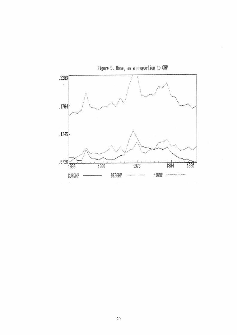
the results for all three. Finally, Figure 5 in the Appendix shows four different measures of the money supply as a proportion of GNP. All four ratios display, to varying degrees, some votality over the period 1960-90. In the case of GNPM /2 there appears to be a slight upward trend

whereas in the case of the other three ratios no discernable trend is obvious either from the plots or from the data. What is interesting, however, is that GNPMGNPC /1,/

and GNPM /2 show sudden increases during the periods 1963-64 and 1974-75. In

9

the case of GNPD/ the turning point in 1963-64 follows the direction of the other three

ratios but is less dramatic. For the period 1974-75 it shows no sudden increase, though there is some upward movement during 1975-76. The two periods 1963-64 and 1974-75 were periods of political turmoil and economic disruption. Intercommunal strife between the Greek and Turkish communities in 1963-64 and Turkey’s invasion of the island in 1974 resulted in a fall in GNP9, thus accounting for the increase in the money/GNP ratios.

4. EMPIRICAL MODELS AND RESULTS Estimates for Cyprus are derived using Tanzi’s methodology as described in Section 2. To recap this involves two stages. First, econometric estimates are obtained for the appropriate measure of money ratio in the observed economy. Using the results from this first stage we then proceed to obtain estimates of the stock of money in the underground economy. Multiplying these estimates by the income velocity of circulation we obtain estimates of the size of the underground economy. Several empirical models were estimated based on the following general relationship: Dependent Variable = );;/;/( PGNPRYWSYTf (9)

where T is a measure of income tax, Y is national income, WS is wages and salaries, R is an appropriate rate of interest and PGNP represents per capita .GNP Following Tanzi (1983) we tried both translog and semi-log specifications. We also estimated equations in simple level terms. Equation (10) below, estimated for the period 1960-90 using OLS, represents our best results:

PGNPADRYWSYTMC 17.092.3)/(86.0)/(81.394.1)2/(ln −−++−= (10)

)33.12()47.3()09.7()71.3()32.25( −−−

0735.0)24,1(:0817.0)24.1(:0339.0 === FFFFSCSER

1951.5)28,1(:4379.0)2(:9582.0 22 === FHXNR

10

ADR is the average deposit rate. A dummy with value 0 for the period 1960 – 1973 and 1 for the period 1974 – 1990 was included to capture changes in the pre and post-Turkish invasion period. The reported coefficients and t-statistics (given in parentheses) have been rounded to two decimal places. SER is the standard error of the regression; SC is the F version of a Lagrange Multiplier test for first order serial correlation; FF is Ramsey’s RESET test for functional form, which involves regressing the residuals on the square of the fitted values; N is a skewness – kurtosis test for normality; and H is the F version of a test for heteroscedasticity which involves regressing the squared residuals on squared fitted values. All the variables in equation (10) are statistically significant at the 5% level and all have the correct sign. The SC,FF and N tests are satisfied at the 5% level but the H test passes only at the 1% level. Equation (10) also passes the Chow-test for stability which is obtained by splitting the estimation period into two sub-periods and then applying the OLS procedure to each sub-period. The stability results are shown in equations (11) and (12) below: 1960 – 1973

PGNPADRYWSYTMC 01.029.6)/(24.1)/(61.203.2)2/ln( −−++−= (11)

)01.0()44.0()99.1()07.2()68.7( −−−

7577.0)9,16(:2160.1)20,5(:2183.8)12,1(:5913.0)2(:8905.0

8215.2)8,1(:0029.0)8,1(:0368.022

=====

===

FPFCFHXNRFFFFSCSER

1974 – 1990

(12)

)38.7()94.1()19.1()90.2()40.9( −−−

0169.0)8,1(:9507.1)10,1(:0298.0 === FFFFSCSER

2878.1)12,1(:4522.0)2(:9655.0 22 === FHXNR

C is the Chow-test which passes at the 5% level and P is Chow’s second test for adequacy of predictions and also passes at the 5% level. The stability of the equation is also verified from plots of the CUSUM (Cumulative Sum) and CUSUMQ (Cumulative Sum of Squares) tests10 .

PGNPADRYWSYTMC 23.065.5)/(41.0)/(84.1089.1)2/(ln −−++−=

11

The results of equation (11) satisfy all the diagnostic tests at the 5% level with the exception of the H test which passes at only the 1% level. The estimates for the period 1974-90, equation (12), pass all the diagnostic tests at the 5% level. Estimates using DC/ and 1/MC as dependent variables produced unacceptable

results. Examples of these are shown by equations (13) and (14).

PGNPADRYWSYTDC 19.072.14)/(43.1)/(43.014.1)/ln( −−+−−= (13)

)80.6()15.5()87.5()21.0()37.7( −−−−

0709.1)28,1(:3483.1)2(:7756.08348.3)24,1(:1786.13)24,1(:0682.0

22 ===

===

FHXNRFFFFSCSER

PGNPADRYWSYTMC 097.026.7)/(73.0)/(26.027.1)1/ln( −++−− (14)

)82.6()05.5()97.5()25.0()26.16 −−

1729.0)28,1(:0972.1)2(:7782.08360.2)24,1(:2727.12)24,1(:0343.0

22 ===

===

FHXNRFFFFSCSER

In both cases the SC test for serial correlation fails at the 5% level, YT/ is insignificant

and the signs for YT/ and ADR are not what we would expect.

Using the results from equation (10) we plot estimated currency holdings against actual values. As can be seen from Figure 6 in the Appendix the fit is very good, especially from 1960 to 1974. Equation (10) gives the logarithm of estimated currency ratio for every year. Given

2M we can calculate the estimated currency holdings )( eC . To see this let

)2/ln( MCX = , then 2lnln MCX −= or equivalently ).2lnexp( MXCe += The actual

and estimated currency holdings are shown in columns one and two of Table 1 in the Appendix. Setting the tax variable in equation (10) equal to zero and following the same procedure, a new estimate of currency holdings )( xC is obtained. The difference

between eC and xC (column 4, Table 1, p.15) is a measure of the excess amount of

money – ‘illegal money’ that people hold presumably to evade taxes. ‘Legal money’ is defined as the difference between M1 and illegal money (column 5). Column 6 shows

12

the income velocity of legal money as the ratio of GNP to legal money. Assuming that the velocities of the observed and underground sectors are the same, an estimate of the underground sector is calculated as the product of the velocity of money and illegal money. These estimates are shown in column 7, whereas column 8 reports the same estimates as a proportion of GNP. 5. CONCLUSION

This paper has attempted to provide estimates of the size of the underground economy in Cyprus. In doing so it has applied a method first developed by Tanzi for the US but supplemented it by subjecting the results to more extensive diagnostic tests. Although several models were estimated using three different dependent variables and specifications, Tanzi’s semi-log specification with the currency ratio, C/M2, as the dependent variable performed best. Based on our preferred model the underground economy in Cyprus for the period 1960-90 is estimated to be between a low 2.7% of GNP (CYP 3.27million) in 1962 and a high 10.3% of GNP (CYP222.9 million) in 1990. Tanzi’s method, as indeed is the case with alternative methods, is not unproblematic. This raises the important question of appropriate criteria for method selection. Two criteria adopted in this paper, which are by no means exclusive or definitive, are as follows: 1) do the available methods provide competing theoretical justifications for their utilisation? and 2) are the available methods constrained by data availability? Beginning with the second criterion first, the existence of more sophisticated approaches which rely on, for example, micro rather than macro data cannot be disputed11 . However, the quality of such data in Cyprus is unreliable. On the question of method selection it has already been stated in Section 1 that none of the available methods are based on a theory of underground economic activity. This raises the related question of whether such a theory can be formulated. The underground economy describes such a varied group of activities that it is doubtful whether an economic theory can be developed which offers an adequate explanation of behaviour by economic agents whose motivation for their actions cannot be reduced to the usual neo-classical motus operandi of utility or profit maximisation12.

13

NOTES

1. These include: cash, casual, clandestine, corrupt, hidden, illegal, illegitimate, informal, irregular, parallel, second, secret, shadow, subterranean, unaccounted, unobserved, unofficial, unrecorded, unreported, and unsanctioned. Feige (1989) presents a taxonomic framework for distinguishing between different meanings of the underground economy.

2. Although economic activity which is unreported may be formally

distinguishable from that which is unrecorded in practice it can be difficult to disentangle the two. Unrecorded income is that part of income which is omitted from the national accounts whereas unreported income usually refers to income omitted from tax returns. The construction of national income figures using inland revenue data will result in unrecording due to unreporting. An added complication for researchers is that while some activities are illegal the income they generate is, nonetheless, recorded in the official statistics. The ‘laundering’ of money is an obvious example.

3. This paper does not pretend to be otherwise.

4. In an interview with the press in the spring of 1991 the Minister of Finance

not only admitted to the existence of a ‘black’ economy but also quoted its size as being in the region of 10% of GDP. This figure has also been mentioned by the island’s two trade union federations, PEO, SEK.

5. See Thomas (1988) for further elaboration.

6. Ibid.

7. The small decline in the face of political instability is not so surprising if we

assume that cash is likely to be viewed as the most liquid and hence least risky form of wealth. Indeed one could argue that under such circumstances per capita currency should, ceteris paribus, increase rather than decrease.

8. For a summary of explanations relating to movements in the currency ratio,

albeit in the UK, see Beenstock (1989), pp. 470-472.

9. GNP declined from CYP121.8 million in 1963 to CYP112.3 million in 1964 and from CYP316.5 million in 1974 to CYP271.2 million in 1975.

14

10. See Brown et al (1975). The plots are available from the authors.

11. Working within the neo-classical paradigm Frey (1989) provides an outline of

how the criminal aspects of underground economic behaviour might be modelled. Thomas (1988), in contrast, suggests a multidisciplinary approach may provide the appropriate route to an understanding of underground activity in general.

15

Appendix

16

17

18

19

20

21

22

Table 1 - Estimates of Informal Economy

YEAR CUR (C) (1)

ECUR (Ce) (2)

ECURT (Cx) (3)

IM (4)

LM (5)

VLM (6)

UE (7)

UEGMP (8)

1960 1961 1962 1963 1964 1965 1966 1967 1968 1969 1970 1971 1972 1973 1974 1975 1976 1977 1978 1979 1980 1981 1982 1983 1984 1985 1986 1987 1988 1989 1990

7.8900 8.7600 9.0300 9.4800

10.9000 11.7200 12.2000 13.6300 15.4900 17.1900 18.4200 21.7600 26.2700 29.7400 35.7500 35.2300 40.8200 44.6700 52.7300 63.9900 75.9500 89.5100 101.6400 115.8600 122.2200 127.8800 130.6700 142.5800 157.6400 169.0800 183.5300

7.7645 8.2415 9.0955 9.5605

11.6128 11.3906 12.7754 13.7031 14.9989 16.8655 18.9296 21.6221 25.4730 29.4612 34.6350 38.1205 41.4522 46.7687 54.1979 63.3424 74.0715 86.8312 99.4434 111.8643 118.6372 128.4990 134.2989 143.7329 156.7022 170.1227 187.5380

6.4585 7.5266 8.5786 9.0220

10.1509 10.4141 11.1666 12.1429 13.6239 15.1360 16.7814 19.5346 23.0251 26.0296 30.7293 34.2609 37.9038 42.4775 48.0463 55.2423 63.5457 74.5871 84.5678 92.4338 97.3880 103.9607 109.4965 116.6858 126.4205 134.7332 146.4783

1.3060

.7149 .5169 .5385 1.4619 .9765 1.6088 1.5602 1.3750 1.7295 2.1482 2.0875 2.4479 3.4316 3.9057 3.8596 3.5483 4.2912 6.1515 8.1001 10.5258 12.2441 14.8757 19.4304 21.2491 24.5383 24.8024 27.0471 30.2817 35.3894 41.0597

13.5940 16.3051 18.4231 19.8415 20.7681 23.4735 24.3312 27.5898 31.3150 36.2905 40.4318 44.6325 55.0021 57.4184 61.8143 58.0484 75.7617 81.1688 94.0185

118.7799 141.7442 175.1259 202.1043 228.6896 238.6109 261.0717 258.5776 289.2029 329.6983 349.4606 398.7903

6.9295 6.3600 6.3236 6.1387 5.4073 6.0025 6.2019 6.2813 5.9939 5.9933 5.7875 6.0404 5.5634 5.9389 5.1202 4.6720 4.5907 5.4442 5.6021 5.4883 5.5523 5.1563 5.2221 5.0658 5.7064 5.7708 6.2832 6.2451 6.1380 6.5120 6.3364

9.0500 4.5465 3.2687 3.3058 7.9050 5.8615 9.9776 9.8004 8.2414

10.3656 12.4326 12.6097 13.6188 20.3795 19.9977 18.0319 16.2893 23.3622 34.4614 44.4558 58.4417 63.1343 77.6816 98.4311 121.2548 141.6061 155.8388 168.9118 185.8699 230.4573 260.1711

.0961 .0438 .0281 .0271 .0704 .0416 .0661 .0566 .0439 .0477 ,0531 .0468 .0445 .0598 .0632 .0665 .0468 .0529 .0654 .0682 .0743 .0699 .0736 .0850 .0891 .0940 .0959 .0935 .0918 .1013 .1030

23

24

REFERENCES Acharya, S. (1984) “The Underground Economy in the United States: Comment on Tanzi”

Staff Papers, International Monetary Fund, No. 31, December, pp. 742-746. Beenstock, M. (1989) “The Determinants of the Money Multiplier in the United Kingdom”,

Journal of Money, Credit and Banking, Vol. 21, No. 4, pp. 465-480. Bhattacharyya, D.K. (1990) “An Econometric Method of Estimating the ‘Underground

Economy’ United Kingdom (1960 – 1984): Estimates and Tests” Economic Journal, Vol. 100, No. 402, September, pp. 703-717.

Brown, L., J. Durbin and J. Evans (1975) “Techniques for testing the constancy of regression

relations over time”, Journal of the Royal Statistical Society, 37, pp. 149-92. Cagan, P. (1958) “The Demand for Currency Relative to the Total Money Supply”, Journal of

Political Economy, 66, pp. 303-328. Economic Report 1989, Department of Statistics and Research, Ministry of Finance, Nicosia,

Republic of Cyprus. Feige, L. (1979) “How Big is the Irregular Economy?”, Challenge, 22, pp. 5-13. ____________ (1980) “A New Perspective on Macroeconomic Phenomena – the Theory and

Measurement of the Unobserved Sector of the United States: Causes, Consequences, and Implications”. Mimeo.

____________ (1986) “A Re-examination of the ‘Underground Economy’ in the United

States: A Comment on Tanzi”, Staff Papers, International Monetary Fund, Vo. 33, No. 4, pp. 768-781.

____________ (ed) (1989) The Underground Economies: Tax Evasion and Information

Distortion, Cambridge University Press. ____________ (1989) “The Meaning and Measurement of the Underground Economy” in

Feige (ed) (1989), pp. 13-56. ____________ (1989) “How Large (or Small) should the Underground Economy Be?” in

Feige (ed) (1989), pp. 111-126. Guttman, M. (1977) “The Subterranean Economy”, Financial Analysts Journal, 34, pp. 24-27.

25

International Financial Statistics Yearbook 1990, International Monetary Fund, Washington. International Financial Statistics, February, 1991, International Monetary Fund, Washington. Matthews, K. (1982) “Demand for Currency and the Black Economy in the U.K.”, Journal of

Economic Studies, 9, pp. 3-22. Pissarides, C. and Weber, G. “An Expenditure - Based Estimate of Britain’s Black Economy”

Journal of Puplic Economics, Vol. 39, No 1, pp 17-32. Porter, D. and Bayer, S. (1989) “Monetary Perspective on Underground Economic Activity in

the United States” in Feige (Ed) (1989), pp. 129-157. Statistical Abstract 1987/88, Department of Statistics and Research, Ministry of Finance,

Nicosia, Republic of Cyprus. Tanzi, V. (1980) “The Underground Economy in the United States: Estimates and

Implications”, Banco Nazionnale del Lavoro Quarterly Review, 135, pp. 427-453. _____________ (1983) “The Underground Economy in the United States: Annual Estimates,

1930-80” Staff Papers, International Monetary Fund, pp. 283-305. ______________ (1984) “The Underground Economy in the United States: Reply to

Acharya”, Staff Papers, International Monetary Fund, pp. 747-750. Thomas, J. (1986) “The Underground Economy in the United States: Comment on Tanzi”,

Staff Papers, International Monetary Fund, Vol. 33, No 4, pp. 782-788. _________ (1988) “The Politics of the Black Economy”, Work, Employment & Society, Vol. 2,

No. 2, pp. 159-190. _________ (1989) “Indirect Monetary Measures of the Size of the Black Economy: A

Sceptical Note”, Mimeo.