Diploma Thesis The Unfolding Pathway of Ubiquitin in various chemical environments Florian Dommert Ludwigs-Maximilians University Munich Chair for Applied Physics Prof. Dr. Hermann E. Gaub July 2007
Figure 1.1: Sequence and secondary structure of ubiquitin. The tertiary structure
of the protein mainly arises from the arrangement of the strands β1 to
β5, the α-helix, and the two 310-helices. Figure adapted from [9].
not start until 80 ◦C and is almost pH-independent [10, 11]. Further structural stability
is provided by a dense hydrogen bonding pattern, due to a high amount of secondary
structure elements. Additional to the hydrogen bonds connecting the residues of the
α -helix and the β -strands, the backbone nitrogen atoms of the residues 23 and 24 form
hydrogen bonds with the carbonyl oxygen atoms of the residues 52 and 54. Furthermore
hydrogen bonds between the backbone nitrogen atoms of the residues 56 and 57 and
the carbonyl oxygen atoms of the residues 18 and 21 strengthen the tertiary structure.
We aim at analyzing the unfolding pathway of ubiquitin in different urea concentra-
tions with MD simulations, which allow direct observation of the unfolding process on
the atomic level. Application of different methods to stress the protein by modelled
mechanical forces, enables us to compare the unfolding events with the time course of
the forces and their influence on the unfolding process. This is expected to gain insight
into the Gibb’s free energy landscape. Furthermore with the addition of the denaturant
urea we want to derive information about its influence on the unfolding process and its
interaction mechanism with the solvent and the protein. To this end we will analyse
the course of the secondary structure, the energetics of the hydrogen bonds, providing
9
1 Introduction
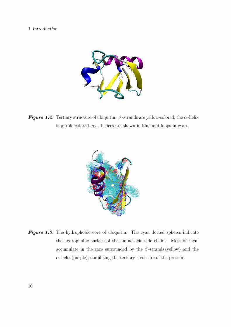
Figure 1.2: Tertiary structure of ubiquitin. β -strands are yellow-colored, the α -helix
is purple-colored, α310 helices are shown in blue and loops in cyan.
Figure 1.3: The hydrophobic core of ubiquitin. The cyan dotted spheres indicate
the hydrophobic surface of the amino acid side chains. Most of them
accumulate in the core surrounded by the β -strands (yellow) and the
α -helix (purple), stabilizing the tertiary structure of the protein.
10
information about a change of the enthalpic part of G, and the surface of the residues
accessible to the solvent, that helps to get an idea about a changing entropy of the
system.
11
2 Methods
2.1 Molecular Dynamics Simulations
Molecular Dynamics (MD) studies aim at elucidating processes at the atomic level.
They enable us to obtain information about many physical quantities that are difficult
or impossible to access experimentally. Particularly examinations of biological systems
like a solvated protein, can be refined with the help of computer simulations. However,
some problems arise: the creation of an accurate model, the sampling of the configu-
rational space of the investigated protein and the the limited computational resources
that restrict the size of the simulation system. This chapter describes the basics of MD
simulations and our way to adress the problems mentioned above.
One main concern in MD simulations is the reduction of the computational cost. To
this end several possibilities exist, which affect the accuracy of the model in different
ways. Major difference arises in the model for the interaction of the protein with its
environment. Here two different possibilities are available; either the interaction bet-
ween protein and solvent is included in a model of the protein (implicit solvent) or the
interaction between protein and solvent in a simulation is explicitly calculated (explicit
solvent). The first method considerablely reduces the computational effort, but the
results strongly depend on the protein model. As the interaction of urea with the
protein and water is not clear at all, we used an explicit solvent model. Furthermore
this model allows a more precise description, but the computational cost is much higher,
12
2.1 Molecular Dynamics Simulations
due to the explicit treatment of the solvent molecules. Accordingly, the simulation
times with explicit solvent are restricted to the nanosecond timescale.
2.1.1 Principles
To gain an atomic description of a protein motion, the Schrodinger equation for the
system has to be solved:(Te + TK + Ve + VK + VeK
)Ψ = i · ~ ∂
∂tΨ, (2.1)
with Ψ = Ψ(~x1, ..., ~xNe , ~X1, ..., ~XNK
).
The vectors ~xi ∈ R3, (i ∈ {1...Ne}), and ~Xj ∈ R3, (j ∈ {1...NK}) denote the positions
of the electrons with mass me and nuclei with mass MK , respectively, the operator for
the kinetic energies T for the electrons is,
Te =−~2
2
Ne∑i=1
1
me
∂2
∂ ~xi2 , (2.2)
and for the nuclei
TK =−~2
2
NK∑j=1
1
MK
∂2
∂ ~X2j
. (2.3)
The operators Ve = Ve (x1, ..., xNe) and VK = VK(X1, ..., XNK) describe the potential
energy V in terms of the coordinates of the electrons and nuclei, respectively, arising
from their interaction among each other. To include the energy, that results from the in-
teraction between eletrons and nuclei the operator VeK = VeK (x1, ..., xNe , X1, ..., XNK)
is present.
For all but the most simple cases the Schrodinger equation cannot be solved analyti-
cally, therefore since its introduction in 1927 theoretical physics searches for appropiate
approximations [12]. Until M.Born and R. Oppenheimer provided a more rigorous ex-
planation [13], a separability of the wavefunction Ψ in χ(X1, ...XNK) and ϕ(~x1, ..., ~xNe)
was justified with the thermodynamic equipartition of the velocities of the electrons
13
2 Methods
and nuclei. Due to the strongly differing masses of electrons and nuclei, their velocities
scale with√
me
mK. For this reason the reaction of the electrons, following a movement
of the nuclei, is assumed to be instantaneous. Hence, a description of the molecule in
its center of mass system with a wavefunction separated in a function of the nucleus
coordiantes and a function of the electron coordinates, parametrized by the nucleus
coordinates is justified. Finally an orthogonal transformation can be found, yielding
the complete separability of the the coordinates of the electrons and nuclei in the wave-
function. It should be mentioned that the calculations of M. Born and R.Oppenheimer
do not only explain the separability of the wavefunctions, they firstly predicted the or-
der of the energy spectrum from a diatomic molecule by its vibrational and rotational
modes. For our aims the separability of the wavefunction allows us to treat the motion
of the considered atoms with the coordinates of their nuclei.
Another approximation is to describe the potential V of our examined system in
mathematically simple terms to obtain an easily computable and parametrized expres-
sion, the so called force field. The potential energy V and the resulting forces ~Fk
mainly depend on the Coulomb, Van der Waals, and intramolecular interactions, that
are defined by the bond configuration of the molecule. Due to the long range interac-
tion character of the Coulomb forces, their calculation turns out to be the most time
consuming part of the computations.
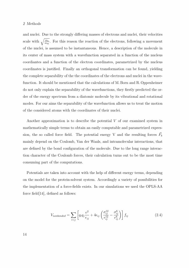
Potentials are taken into account with the help of different energy terms, depending
on the model for the protein-solvent system. Accordingly a variety of possibilities for
the implementation of a force-fields exists. In our simulations we used the OPLS-AA
force field[14], defined as follows:
Vnonbonded =∑i<j
[qiqj
e2
rij
+ 4εij
(σ12
ij
r12ij
−σ6
ij
r6ij
)]fij (2.4)
14
2.1 Molecular Dynamics Simulations
fij =
0 pair ij connected by a valence bond or a valence bond angle
0.5 1,4 interaction (separated by exactly 3 bonds)
1.0 otherwise
Vbonded =∑bonds
Kr (r − req)2 , (2.5)
Vangle =∑
angles
KΘ (Θ−Θeq)2 , (2.6)
Vtorsion = 12
∑i
V1,i [1 + cos(φi)] + V2,i [1− cos(2φi)] +
V3,i [1 + cos(3φi)] . (2.7)
The nonbonded terms include the electrostatic and the Van der Waals interactions,
where fij defines their strength and rules out the directly bonded pairs. Harmonic
potentials approximate the energies, arising from the deviations in the equilibrium
distances req and equilibrium angles Θeq of the bond conformations. The dihedral
configuration energy (2.7) depends on the potentials V1,i, V2,i, V3,i of the bonded atoms
i. In contrast to force-fields, using only a single term for the diheral configuration
energy, the three terms allow a more accurate description of the energy.
The third important approximation in MD simulatons is the classical treatment of
the molecular motion. Newton’s second law is applied to the masses of the nuclei and
its numerical integration yields the trajectories of the nuclei in an MD simulation:
MK ·d2 ~XK
dt2= −∂V ( ~X1, ..., ~XN)
∂ ~XK
(2.8)
= ~FK( ~X1, ..., ~XN). (2.9)
In 1967 L. Verlet[15] published a simple algorithm to solve this set of coupled differential
equations by discretizing the time t and expanding up to second order in t:
~XK(t + ∆t) = 2 ~XK(t)− ~XK(t−∆t) +~FK (∆t)2
mK
(2.10)
15
2 Methods
The resulting data of a simulation, integrated over n time steps ∆t, describe the tra-
jectories of the molecules,
~XK(ti), ti = i ·∆t, i = 1, ..., n, (2.11)
providing a possibility to calculate many thermodynamic and mechanic quantities,
not accessible to measurements in experiments. Today most MD program packages
use a modified version of the Verlet algorithm, but the discretization in time and the
expansion up to second order is still the main idea to allow fast and precise computation.
2.1.2 Force Probe Molecular Dynamics simulations
To model the effect of the mechanical stress harmonic potentials, modelling a spring
with spring constant k, are attached to the terminus atoms of the protein (fig. 2.1).
They are moved in a specified direction n with velocity v, hence the potential energy
Vα on the respective atoms is modified by including the term:
Vα,eff(t) =1
2k ·
(~XK(t)− n · v · t
)2
. (2.12)
vpull vpull
Figure 2.1: Setup of an FPMD simulation: Two springs are pulling the termini of
the protein each in opposite directions. This way friction forces arising
from a movement of the protein through the solvent are reduced.
16
2.1 Molecular Dynamics Simulations
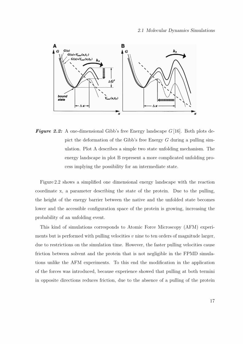
Figure 2.2: A one-dimensional Gibb’s free Energy landscape G [16]. Both plots de-
pict the deformation of the Gibb’s free Energy G during a pulling sim-
ulation. Plot A describes a simple two state unfolding mechanism. The
energy landscape in plot B represent a more complicated unfolding pro-
cess implying the possibility for an intermediate state.
Figure 2.2 shows a simplified one dimensional energy landscape with the reaction
coordinate x, a parameter describing the state of the protein. Due to the pulling,
the height of the energy barrier between the native and the unfolded state becomes
lower and the accessible configuration space of the protein is growing, increasing the
probability of an unfolding event.
This kind of simulations corresponds to Atomic Force Microscopy (AFM) experi-
ments but is performed with pulling velocities v nine to ten orders of magnitude larger,
due to restrictions on the simulation time. However, the faster pulling velocities cause
friction between solvent and the protein that is not negligible in the FPMD simula-
tions unlike the AFM experiments. To this end the modification in the application
of the forces was introduced, because experience showed that pulling at both termini
in opposite directions reduces friction, due to the absence of a pulling of the protein
17
2 Methods
through the solvent. Anyway, the results of the simulations and the experiments are
not comparable directly and an appropriate description of the effect of friction on the
calculated forces is inevitable. A model for a two energy state system [17], describing
the protein unfolding attempt frequency k0 in terms of the reciprocal thermal energy
β = 1kBT
and Kramer’s prefactor[18] ω0, provides an approximation of the attempt
frequency for unfolding:
k0 = ω0 · exp(−β∆G 6=). (2.13)
As an unfolding attempt decreases the probability to find the system in the folded state,
with the assumption of a linear decrease in the barrier height ∆G 6=(t) = ∆G 6=−kvt∆x,
yields a differential equation describing the probability P (t) to find the system in the
native state. In the model ∆x corresponds to the distance between the minimum of G
and the following maximum.
dP (t)
dt= −P (t) · k0(t) (2.14)
= −P (t) · ω0 · exp(−β(∆G 6= − kvt∆x)). (2.15)
This approximation holds as long as ∆G 6=− k · v ·∆x · t � kBT and back reactions are
negligible. Integrating eq. 2.15 yields, regarding the boundary condition P (t = 0) = 1,
to find the system in the folded state:
P (t) = exp
[ω0
βkv∆xe−β∆G6=
(1− eβkvtD∆x
)]. (2.16)
Substituting the rupture force FD = kvtD in eq. 2.16 and differentiating the result in
respect to FD reveals the most probable pulling force Fmax at the time of an unfolding
event, according to dP (FD)dFD
= 0:
Fmax =1
β∆x· ln(
βkv∆x
k0
). (2.17)
For an explicit treatment of the friction forces a linear term with a friction constant γ
is added heuristically:
Fmax = γ · v +1
β∆x· ln
(βkv∆x
k0
). (2.18)
18
2.1 Molecular Dynamics Simulations
Equation (2.18) provides the possibility to extrapolate the computed forces to the
regime, where friction is negligible— the situation given in the AFM experiments—
hence rendering a direct comparison possible.
2.1.3 Force Clamp Molecular Dynamics Simulations
In the previous section was described how to deal with the friction forces and the time-
dependent shift of the Gibb’s free energy G, occuring in FPMD simulations. Both
strongly affect the unfolding mechanism. To minimize their influence on the unfolding
mechanism of the protein, the idea of the Force Clamp experiments was realized in
simulations. Force Clamp experiments are carried out with AFM by pulling the protein
with a cantilever applying a constant force (k0 = const.), yielding a constant overall
decrease of ∆G 6=. To realize this situation in the Force Clamp Molecular Dynamics
(FCMD) simulations, the position of the harmonic potential is calculated and adjusted
every integration step to keep the distance between the potential and the considered
atoms constant. The advantage arises in the improved comparability of experiment and
simulations. Since the constant shift of the Gibb’s free energy that favours unfolding
is realized in nearly identical ways in simulation and experiment, no special analysis
of the friction forces Fγ in the FCMD simulations is required. Additionally in this
kind of simulations unfolding is not dominated by the mechanical deformation of the
tertiary structure, due to the increasing distance of the pulling potentials. Instead, the
denaturation mechanism is based on the lowering of ∆G 6=, which perturbs the native
energy landscape to a lesser extent. Apart from the differences in the method to apply
a force the simulation setup corresponds to the FPMD simulations.
For an FCMD simulation information about the rupture force Frup is required.
FCMD simulations with a force much lower than Frup yield unfolding attempt fre-
quencies k0, which are too low to obtain an unfolding event in a computationally
feasible time-span. An application of a force too strong can yield unfolding pathways
19
2 Methods
of the protein, that are artificial, because of the strongly deformed Gibb’s free energy
landscape.
2.2 The Aquaeous Urea Solution
FPMD and FCMD simulations provide us a tool to denature the protein in a time-span
feasible for computational studies. Additionally, chemical denaturants like urea (fig. 2.3)
reveal a possibility to influence the protein unfolding behavior. Urea is one of the prote-
olysis end products in mammals, some plants and many fungi [19]. The French chemist
Rouelle firstly extracted urea with hot alcohol from evaporated urine in 1773 [20].
Figure 2.3: The urea molecule (H2N)2 CO
Urea is widely used as a denaturant. However, despite its common application it
is not clear how urea influences unfolding. On the one hand, there could be direct
interaction within urea and the protein [7]. This model suggest, that interaction be-
tween the urea molecules and the less polar atoms of the protein backbone provide the
denaturating effect of urea. On the other hand unfolding can be affected by altering of
the solvent environment, due to interaction of urea with water [8]. Several experiments
and MD studies led to two models for the hydrogen bonding dynamics in an aqueous
urea solution, according to which the urea concentration strongly effects the action
mechanism. One model suggests that the urea molecules fit into the hydrogen bond
20
2.3 Simulation Details
network of water. No distortion of the orientational dynamics of the water dynamics
occurs and the entropy of the system stays stable. This model is suitable to describe
low concentrations of urea. At high urea concentration however, the urea molecules
start to interact strongly with each other resulting in a urea aggregation, predicted
by the other model. This narrows the water configurational space decisively with the
effect of lower solvent entropy due to urea aggregation.
In the native state, the tertiary structure of ubiquitin generates a hydrophobic core,
because most of the hydrophobic residues point inwards. Unfolding increases the sol-
vent accessible surface area of these residues and narrows the configurational space of
the water molecules, which lowers the entropy of the solvent. If the stability of ubiquitin
is strongly dependent on the solvent entropy, high urea concentrations should desta-
bilize the protein, due to the lower absolute entropy of the whole system. Otherwise
if the stability of the protein depends mostly on the enthalpic part of the Gibb’s free
Energy a change in urea concentration should not effect the unfolding process much.
In case that the distortion of the hydrogen bonding pattern of the water molecules
in high urea concentration is of major relevance, the question arises whether the dis-
turbed electrostatic environment or a change in the viscosity of the solution influences
the unfolding.
2.3 Simulation Details
The simulations are performed in a box, filled with the protein and a solvent. To
minimize artifacts from the limited system size, periodic boundary conditions (PBC)
are used in the calculation of the forces. The PBC feature a wrapping of the simula-
tion box with copies of itself, allowing an appropriate treatment of the forces by the
minimal image convention (MIC). This convention constrains the number of atoms for
the determination of the potential energy V to the bulk within a box, centered at the
21
2 Methods
position of the atom considered for the integration.
As we use PBC in our simulations, the time consuming calculation of the electrostatic
interaction can be modified to reach faster computation time with only a slight loss in
accuracy. To this aim the calculation of the electrostatic potential is split up. Within
a certain cut-off radius rcutoff the potenial is calculated explicitly. Beyond this radius
the charges are assigned to a grid via an adequate distribution that is subjected to
a Fourier transformation. The two parts of the electrostatic potential converge fast,
because the cut-off radius does restrict explicit calculation to a small space and the
presence of the PBC allows an easily computable expression for the potential in the
reciprocal space, dependent on the used distribution function. This method is an
enhanced Ewald summation[21] and called Particle Mesh Ewald (PME) algorithm[22].
In contrast to an explicit calculation the number of computational operations is reduced
from O(N2) to O (N log N).
All simulations represent an NpT ensemble, so at first the methods to keep the pres-
sure and temperature constant should be explained. To obtain constant temperature
and pressure during the MD simulation all the atoms in the simulation box are coupled
to an external heat bath via a Berendsen thermostat and barostat [23].
A constant temperature requires a constant mean kinetic energy. To this end in every
simulation step the atom velocities are linearly scaled to yield a constant temperature:
v → λ · v, (2.19)
λ =
√1 +
∆t
2τT
(T0
T− 1
). (2.20)
Similarly, the pressure scaling corresponds to a variation of the box size and coordi-
nates. Introducing a pressure coupling constant τP , the transformation for a cubic box
22
2.4 System Setup
with lenght l and the coordinates XK can be written as follows:
~XK → µ ~XK , (2.21)
l → µl, (2.22)
µ = 3
√1− ∆t
τP
(P − P0) . (2.23)
The coupling constants have to be set appropiate to the system size, to take the
energy flux through the system into account. For our setup we choose τP = 1ps and
τT = 0.1 ps.
2.4 System Setup
Ubiquitin renders a good simulation system, due to its small size of 76 residues. For
this reason no big simulation box is required and the computational resources allow
simulations on the nanosecond timescale. Additionally, a structure model, obtained
from a x-ray diffraction pattern, exists[11], containing structure information about the
individual residues with a resolution of 1.8 A. These conditions alleviate the set up of
a realistic simulation system in several steps.
First the crystal structure of the protein has to be solvated in a simulation box. To
this end we chose a water model, suitable for the applied force field. Our choice, the
TIP4P model water consists of two hydrogens, one oxygen, and an additional charged
dummy atom to approximate the water dipole moment more accurately. In this case
our simulation setup differs from the methods of [1], but this change is required to
achieve comparability of the interaction in the solvent with the results of [7].
The simulation box was cubic and of 5.9 nm length filled with about 5000 TIP4P
water molecules. Finally to get a physiological environment, we added sodium and
chloride ions to obtain a 150mM NaCl solution.
The x-ray-scattering method does not provide information about the protonation
23
2 Methods
Figure 2.4: TIP4P water model. The coloured grid illustrates the electrostatic influ-
ence of the different atoms. In addition to the two hydrogens (blue) and
the oxygen (red), an added dummy atom (green) provides an improved
approximation of the water dipole moment.
states of the native state of the protein. To overcome this problem we used the program
packages WHAT IF [24] and Delphi. They enable us to calculate the electrostatic
potentials at the residue sites and the pKa in the solution, resulting in information
about the protonation states of the protein. We found the histidines being in the
protonated state.
Now the protein is ready for further steps preparing the producing simulations.
To obtain a solved protein from the crystal structure, surrounded by water, sodium,
and chloride ions, first we minimized the potential energy of the crystal structure
via a Monte-Carlo method. This deepest descent energy minimization scans the di-
hedral configurational space of the protein to reach a minimum in the potential en-
ergy (fig. 2.5 ). As yet the water molecules are positioned uniformly with random ori-
entations, but are not necessarily thermally equilibrated. To reach the thermal equi-
librium within the solvent molecules, the next preparation step aims at a uniform
distribution of the solvent molecules only affected by the presence of the protein. To
24
2.4 System Setup
0 20 40 60 80 100 120 140!3.4
!3.2
!3
!2.8
!2.6
!2.4
!2.2
!2 x 10⁵
time (ps)
pote
ntia
len
ergy
(k
Jm
ol)
Figure 2.5: During a deepest descent energy minimization the potential energy of
the whole system is converging to a minimum.
0 100 200 300 400 500
!2
!1!1
x 105
time (ps)
pote
ntia
len
ergy
(k
Jm
ol)
0 100 200 300 400 500
2.5
4.5
x 104
kine
tic
ener
gy(
kJ
mo
l)
Figure 2.6: Potential (blue) and kinetic (green) energy of the system in the simulation
during the equilibration of the water. The increase in kinetic energy the
potential energy is decreasing, corresponding to the equilibration of the
solvent.
25
2 Methods
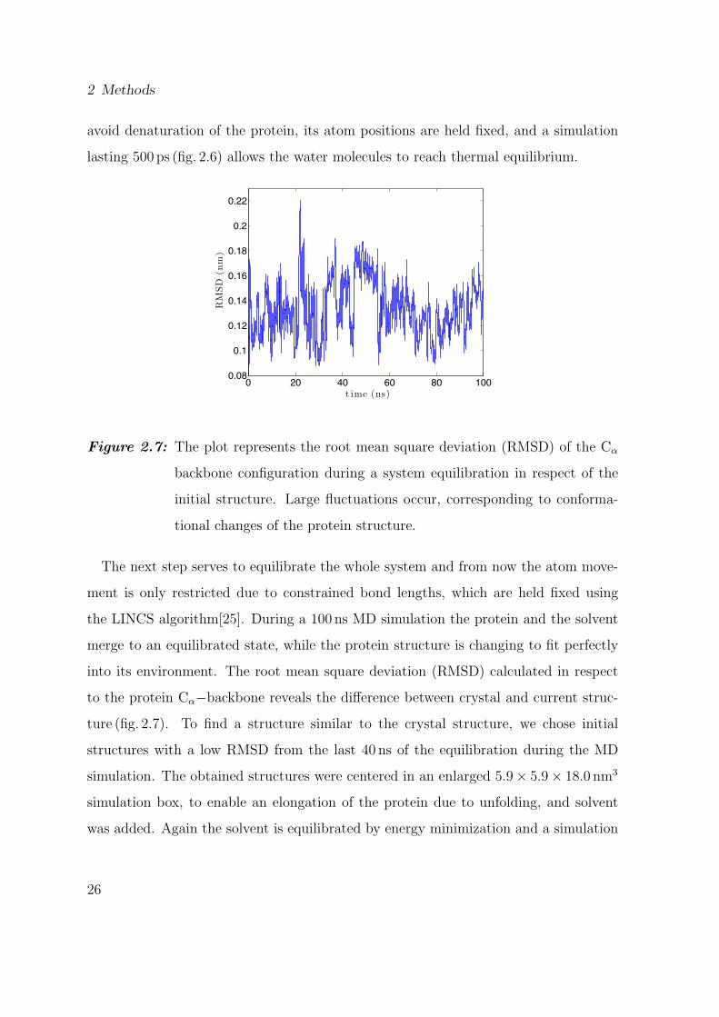
avoid denaturation of the protein, its atom positions are held fixed, and a simulation
lasting 500 ps (fig. 2.6) allows the water molecules to reach thermal equilibrium.
0 20 40 60 80 1000.08
0.1
0.12
0.14
0.16
0.18
0.2
0.22
t ime (ns)
RM
SD
(nm
)
Figure 2.7: The plot represents the root mean square deviation (RMSD) of the Cα
backbone configuration during a system equilibration in respect of the
initial structure. Large fluctuations occur, corresponding to conforma-
tional changes of the protein structure.
The next step serves to equilibrate the whole system and from now the atom move-
ment is only restricted due to constrained bond lengths, which are held fixed using
the LINCS algorithm[25]. During a 100 ns MD simulation the protein and the solvent
merge to an equilibrated state, while the protein structure is changing to fit perfectly
into its environment. The root mean square deviation (RMSD) calculated in respect
to the protein Cα−backbone reveals the difference between crystal and current struc-
ture (fig. 2.7). To find a structure similar to the crystal structure, we chose initial
structures with a low RMSD from the last 40 ns of the equilibration during the MD
simulation. The obtained structures were centered in an enlarged 5.9× 5.9× 18.0 nm3
simulation box, to enable an elongation of the protein due to unfolding, and solvent
was added. Again the solvent is equilibrated by energy minimization and a simulation
26
2.4 System Setup
with restrained protein atom positions.
Finally the system is in an equilibrated state and prepared for the actual investi-
gations. As mentioned we intend to unfold ubiquitin by applying mechanical force
in several solvent environments. To this end after the selection of the three starting
structures the described equilibration process for the solvent has been performed using
a 3M, 7M, and 9M urea solution in addition to the pure water box.
Figure 2.8: Simulation box containing the protein (black) and about 18000 solvent
molecules, depending on the urea concentration. For further FPMD
and FCMD simulations, twelve different structures with variable solvent
concentration and protein conformation were used.
Each of the twelve structures was subjected to an FCMD simulation applying 500 pN
force to the Cα terminus atoms for 18 ns. This simulation setup was expected to be
adequate to observe an unfolding process [1] in respect to the simulation time and the
applied force. The pulling was carried out in two opposite directions parallel to the
z-axis, where most space is available. In contrast to a setup applying only one pulling
potential to a bound protein, our setup reduces the occurring friction forces. In the
different FPMD simulation the direction of the force was kept the same, but the spring
modelling the potential was moving with different velocities of 1, 2, 5 and 10 ms. It
is expected that under these conditions the protein changes from the native folded to
27
2 Methods
the unfolded state. Further, ten FPMD simulations with the same structure in pure
water were performed to analyze the variance of the rupture force and alleviate error
estimation for the force extrapolation.
For our simulations we used a modified code of the MD program package GROMACS
3.3.1 [26]. Because of mechanisms concerning the Fourier transformation in the PME
algorithm GROMACS was compiled with the same FFTW2 library [27] like F.Grater [1]
to maintain comparability, despite longer computation times.
MD simulations produce a huge amount of data and FPMD additionally maintain
information about the spring position. However, GROMACS does not provide a tool
for the analysis of the spring positions. To this end and to provide an efficient way
for handling the data a tool in the C-language was written using the Message Passing
Interface (MPI) [28]. To visualize the trajectories of the molecules VMD [29] was used.
2.5 Analysis Methods
2.5.1 Secondary structure determination
Maps of the change of the secondary structure in time provide information about the
dynamics of the hydrogen bonds, not accurately accessible from direct observation. For
our analysis we used the established DSSP algorithm [30] , which localizes the motifs
by calculating the electrostatic energies between the according elements of the protein
backbone. To this end a partial charge q1 = 0.42 e and −0.42 e is assigned to the carbon
and oxygen, respectively, and a partial charge q2 = 0.20 e and −0.20 e is assigned to
the hydrogen and nitrogen, respectively, followed by a straightforward calculation of
the energy E:
E = f · q1q2 ·{
1
rON
+1
rCH
− 1
rOH
− 1
rCN
}. (2.24)
28
2.5 Analysis Methods
The units of the radii are in A and f = 1390 AC2 is a dimensional factor yielding the
energy unit of kJmol
. For E < −2.1 kJmol
, a hydrogen bond between the corresponding
atom groups is identified and finally, the secondary structure of the protein is derived
from the configuration of these hydrogen bonds.
2.5.2 Hydrogen Bond Energies
To calculate hydrogen bond energies between arbitrary atoms of the simulation system,
we used the established method in [31], based on the distance d in A between the
proton donor and proton acceptor:
EHB = −1
2
(50 · 103 kJ
mol
)· e−36d. (2.25)
2.5.3 Contact Maps
Contact maps were obtained by averaging the distance between the residues over a
time window of 1 ns. Complementing the secondary structure maps, the contact maps
provide information about the orientation of the different secondary structure motifs.
2.5.4 Solvent Accessible Surface Area
Calculation of the solvent accessible surface area of the protein bases on the Double
Cubic Lattice Method [32]. Firstly, the algorithm divides the volume around the pro-
tein into cubic boxes, which only contain one protein atom, treated as a sphere. By
projection of the overlapping spheres onto the surface of the cubes, the surface accessi-
ble to the solvent is calculated. An implementation of this algorithm is present in the
used MD programm package GROMACS, which we use for our analysis.
29
3 Results and Discussion
3.1 The Force Profile of Ubiquitin in the FPMD
simulations
The resulting force profile (fig. 3.1) of an FPMD simulation and a comparsion with
the time course of the simulation allows to identify rupture events and relate them
to involved residues. Figure 3.1 shows a typical force profile and illustrates the main
features of the performed simulations.
For the reaction coordinate, the end to end distance of the pulled atoms was chosen to
provide an appropiate description for the state of the protein, allowing the comparison
of FPMD simulations with different pulling velocities.
As can be seen in figure 3.2 A-C, the rupture forces in 0M, 3M, 7M, and 9M urea-
water solution only slightly differ. Raising the pulling velocity vpull from 1 ms
to 5 ms
increases the maximum force by about 250 pN. However, increasing the velocity fur-
ther to 10 ms
does not reveal drastic changes. In contrast, in the course of an unfolding
process the decrease of the force after the maximum is less pronounced for higher vpull.
Figure 3.2D depicts the scattering of the maximum forces, occuring in FPMD simu-
lations with a pulling speed of 10 ms. It reveals the strong influence of the starting
structure on the time course of the simulations. For the 0M environment, one struc-
ture could not be analyzed due to an error in the simulation setup pulling in wrong
directions, hence only two results are available for a discussion.
30
3.1 The Force Profile of Ubiquitin in the FPMD simulations
0 500 1000 1500 2000 2500 3000 35000
100
200
300
400
500
600
700
800
900
time (ps)
forc
e(p
N)
event 2
event 3
event 1
event 4
event 5
Figure 3.1: Force profile resulting from an FPMD simulation in pure water with a
pulling velocity of 1 ms. The encircled areas mark the different charac-
teristic rupture events of the unfolding process, described in fig. 3.6.
The rupture force peak seems to be slightly increased in case of a low 3M urea
concentration. Though, a further increase of the concentration weakens this effect or
the effect even vanishes. However, urea is known as a denaturant, implying a decrease
of the rupture force with increasing urea concentration, an effect not observable in the
force profiles of our simulations.
To estimate the error or the variance in our model ten FPMD simulations in water
solution were performed, differing only in the distribution of the starting velocities of
the particles corresponding to Poisson-Boltzmann. A pulling speed of 10 ms
was applied
to minimize the required computation time. Figure (3.3) presents the results of the ten
runs. The trajectories elucidate the occurring trend of the force. The rupture events
31
3 Results and Discussion
4 6 8 10 12 140
500
1000
1500
Distance (nm)
Forc
e(p
N)
0M
3M
7M
9M
4 6 8 10 12 140
500
1000
1500
Distance (nm)
Forc
e(p
N)
0M
3M
7M
9M
4 6 8 10 12 140
500
1000
1500
Distance (nm)
Forc
e(p
N)
0M
3M
7M
9M
A B
C D
vpull = 1 ms vpull = 5 m
s
vpull = 10 ms vpull = 10 m
s
0M 3M 7M 9M0
500
1000
1500
2000
2500
Forc
e(p
N)
urea concentration
Figure 3.2: Force vs. distance plots. Plots A to C illustrate the dependence of the
forces due to a change of vpull and the urea concentration. Plot D depicts
the scattering of the rupture forces for different structures obtained with
vpull = 10 ms.
32
3.1 The Force Profile of Ubiquitin in the FPMD simulations
1000
pN
50 ps
Time (ps)
Ruptu
reForc
e(p
N)
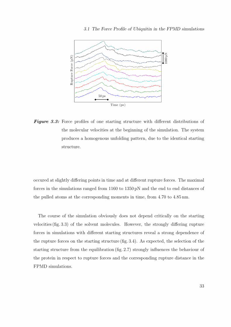
Figure 3.3: Force profiles of one starting structure with different distributions of
the molecular velocities at the beginning of the simulation. The system
produces a homogenous unfolding pattern, due to the identical starting
structure.
occured at slightly differing points in time and at different rupture forces. The maximal
forces in the simulations ranged from 1160 to 1350 pN and the end to end distances of
the pulled atoms at the corresponding moments in time, from 4.70 to 4.85 nm.
The course of the simulation obviously does not depend critically on the starting
velocities (fig. 3.3) of the solvent molecules. However, the strongly differing rupture
forces in simulations with different starting structures reveal a strong dependence of
the rupture forces on the starting structure (fig. 3.4). As expected, the selection of the
starting structure from the equilibration (fig. 2.7) strongly influences the behaviour of
the protein in respect to rupture forces and the corresponding rupture distance in the
FPMD simulations.
33
3 Results and Discussion
0 500 1000 1500 2000 2500 30000
200
400
600
800
1000
1200
1400
Time (ps)
Forc
e(p
N)
structure 1
structure 2
structure 3
Figure 3.4: Force vs time plot gained from FPMD simulations (vpull = 1 ms) in a 9M
urea solution.
3.2 Force fit from the FPMD simulations
To extrapolate the occuring friction forces to a regime, comparable with AFM experi-
ments, we choose pulling velocities vpull = 1, 2, 5 and 10 ms. A Non Linear Least Squares
fit of the maximum forces, averaged over the three starting structures, to eq. 2.18, cor-
responding to the first dissociation event in the course of unfolding, and the pulling
velocities should provide the friction γ and k0 as well as ∆x in the different solvent
environments.
All FPMD simulations, performed with equal velocity and urea concentration, reveal
a strong variance in the observed rupture force. Unfortunately, the number of the
simulations did not suffice to gain a reliable average of the rupture forces and fit them
using the model resulting in eq. 2.18. Furthermore, fig. 3.5 reveals, that all simulations
have been performed in the high friction regime, rendering an appropiate extrapolation
to the low friction regime impossible. As can easily be seen from the plot, already small
changes in the data lead to strongly differing values for the friction constant γ, k0, and
34
3.2 Force fit from the FPMD simulations
0 2 4 6 8 10 120.9
1
1.1
1.2
1.3
1.4
1.5 x 10⁻⁹
Velocity (m
s)
Forc
e(N
)
Figure 3.5: Force fit to eq. 2.18. The strong variance of the rupture forces renders a
reliable fit impossible.
∆x. To provide an example, omitting a single data point that does not follow the trend
of an increasing force with increasing velocity, can yield negative values for the friction
constant γ, which is not consistent with physical reality.
The application of the high pulling velocities entails very strong friction forces. Due
to the fast deformation of the Gibb’s free energy landscape, kinetically trapped tran-
sition states might arise, because the protein is not in thermal equilibrium with its
solvent environment, causing the extreme high rupture forces. Because of the inability
to extrapolate the rupture forces to the low friction regime comparison with experi-
ments is not possible. However, this result reveal, that in our further analysis of the
FPMD simulations we have to keep the influence of the very strong friction at the back
of our mind.
35
3 Results and Discussion
3.3 The Unfolding Pathway of Ubiquitin
3.3.1 Results of the FPMD simulations
In addition to the rupture forces, also available from experiments, snapshots of the
unfolding process can be obtained and compared to the events from the force pro-
file. Figure 3.6 shows snapshots from a trajectory of an FPMD simulation pulling the
terminal atoms with a velocity of 1 ms
in a water solution. They reveal the stepwise
conformational changes of ubiquitin during the simulation.
The first unfolding event occurs within a time of about 340 ps (fig. 3.6, event 1). The
Cα-turn breaks up and the amino acid chain starting at residue 71 is almost completely
stretched. This turn is contained in the crystal structure of the Protein Database but
does not occur in every starting structure of the FPMD simulation.
In the course of the FPMD simulations the arrangement of the β-strands changes
drastically (fig. 3.6, event 2). Two snapshots taken at 815 and 1000 ps simulation
time highlight the rupture of the protein structure, determined by the arrangement of
β-strands 1 to 5, a α-helix and two 310-helices. This second event leads to a loss of
contact between the loop connecting the β1 and β2 strand and the α helix. Furthermore
the contact between the β1 and β5 strand is lost. This structural change introduces
the separation into two small clusters formed by strandβ1 and β2, and the remaining
secondary structure elements of ubiquitin. The β1- and β5-strand align completely
along the pulling direction, whereas the remainder of the protein maintains its three
dimensional structure.
Further pulling on the terminal atoms separates the two stuctural clusters com-
pletely (fig. 3.6, event 3). The structural change of the β1/β2 cluster concentrates on
the alignment along the pulling direction, whereas the conformational dynamic of the
other cluster is dominated by a rearrangement of β3/β4/β5.
After the partitioning of the two clusters the larger cluster containing the α-helix
36
3.3 The Unfolding Pathway of Ubiquitin
t = 1100 ps t = 1300 ps!4
!5!2
!3!1
t = 1400 ps t = 2000 ps
!5
!3
!4
t = 1000 pst = 815 ps!4
!5
!1!2
!3
Event 4. The parallel alignment of !3 relative to !5 vanishes.
turn!-helix
t = 2500 ps t = 3600 ps
Event 5. The remaining tertiary structure gets lost by a suddendisrupture of the common axis of the !-helix and the turn.
Event 1. The small turn next to the C! atom of the N-terminuslooses its bond conformation due to the pulling
Event 2. Primary partitioning of the protein structure. The core-shaping conformation of the !1, !2 and !5-strand is altered drasti-cally, especially the orientation of !1 relative to !2, and !1 relativeto !5.
Event 3. Separation into a !1/!2 cluster and a cluster of theremaining structure elements is completed.
t = 140 ps t = 480 ps
C! ! turn
N-terminus C-terminus
Figure 3.6: Snaptshots depicting the unfolding in a FPMD simulation with pulling
velocity vpull = 1 ms.
37
3 Results and Discussion
rearranges. The contact between β3 and β5 opens up and instead β3 and β4 align
antiparallel (fig. 3.6, event 4). From now on the unfolding proceeds in a rotation around
the axis formed by the α-helix and the bend between β4 and the blue 310-helix in the
lower part of the figure.
At the end of the FPMD simulations the tertiary structure becomes an uncorrelated
chain of secondary structure elements (fig. 3.6, event 5). The last rupture events destroy
the alignment of the β-strands and the collective axis along the helix and the turn gets
lost. Further pulling yields a complete stretching of the residue chain without any
secondary structure elements.
This unfolding sequence was found in all performed FPMD simulations. Apart from
the first step, which can only arise if the starting contains the bend at the N terminus,
the protein unfolding follows this pathway independent of the urea concentration and
pulling velocity. The points in time of the events differ in the simulations, but the
order of the events remains unchanged and no dependence on the urea concentration
is detectable.
3.3.2 The Unfolding Process in the Force Clamp MD simulations
In contrast to the FPMD simulations a characterization of the unfolding process by
different rupture forces is not possible, due to the constant pulling force. However in
this case the end to end distance of the Cα termini allows a reliable characterization
the state of the protein. In our FCMD simulations we compare in unfolding in pure
water with unfolding in solutions with different urea concentrations (3M, 7M, 9M).
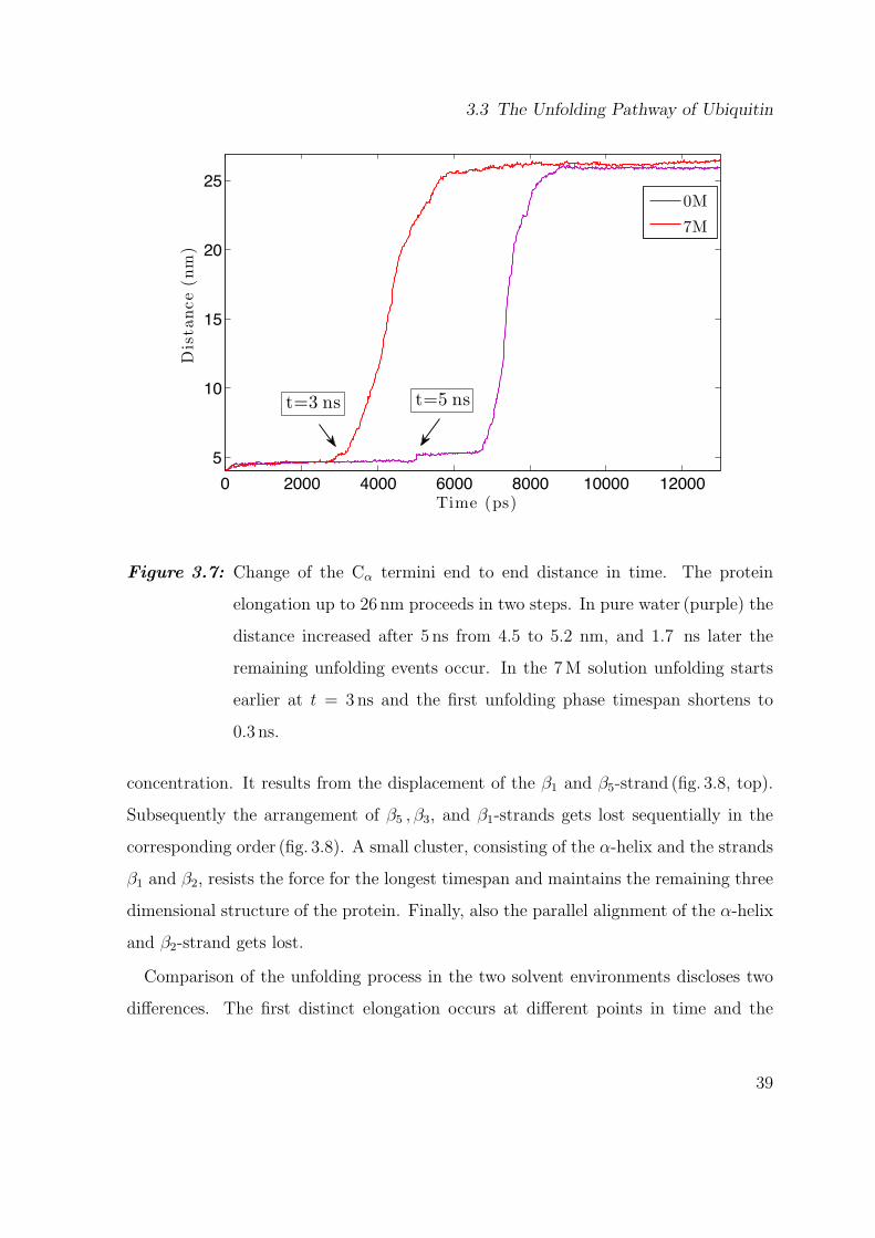
Unfolding was only obtained in pure water and 7M urea solution (fig. 3.7).
The unfolding process in an FCMD simulation proceeds differently compared to the
FPMD simulations. The first event is visible as the step in the end to end distance at
t = 3ns and t = 5ns in the 7M and 0M urea solution, respectively. For the two solvents
this intermediate state lasts for different times tIM; 1.7 ns in 0M and 0.3 ns in 7M urea
38
3.3 The Unfolding Pathway of Ubiquitin
0 2000 4000 6000 8000 10000 120005
10
15
20
25
Time (ps)
Dis
tance
(nm
)0M
7M
t=5 nst=3 ns
Figure 3.7: Change of the Cα termini end to end distance in time. The protein
elongation up to 26 nm proceeds in two steps. In pure water (purple) the
distance increased after 5 ns from 4.5 to 5.2 nm, and 1.7 ns later the
remaining unfolding events occur. In the 7M solution unfolding starts
earlier at t = 3ns and the first unfolding phase timespan shortens to
0.3 ns.
concentration. It results from the displacement of the β1 and β5-strand (fig. 3.8, top).
Subsequently the arrangement of β5 , β3, and β1-strands gets lost sequentially in the
corresponding order (fig. 3.8). A small cluster, consisting of the α-helix and the strands
β1 and β2, resists the force for the longest timespan and maintains the remaining three
dimensional structure of the protein. Finally, also the parallel alignment of the α-helix
and β2-strand gets lost.
Comparison of the unfolding process in the two solvent environments discloses two
differences. The first distinct elongation occurs at different points in time and the
39
3 Results and Discussion
!5
!1
t = 4.5 ns t = 5.3 ns!2
!4
t = 7.2 ns t = 7.4 ns
!-helix
turn
!3
!1
!2
At t = 7.2 ns the main unfolding process of the protein begins. After thedisorientation of the !-helix and the turn, firstly the alignment of "1/"2
vanishes.
During the first slow unfolding event the !1 and !5-sheets are pulled apart.This introduces the decay of the parallel alignment of !1/!2/!5.
Figure 3.8: Snaptshots describing the unfolding in a FCMD simulation in a 0M urea
solution.
duration of the decomposition of β1 and β5 is different. However only two unfolding
events are available for analysis, rendering a meaningful evaluation impossible.
40
3.3 The Unfolding Pathway of Ubiquitin
3.3.3 Comparison of the unfolding pathway in the FPMD and
FCMD simulations
Unfolding of ubiquitin was simulated using two different methods: pulling at the ter-
mini of the protein by a moving harmonic potential (FPMD) and alleviating the un-
folding process by applying a constant force on the termini of the protein (FCMD). It
turned out, that two different unfolding pathways occur, depending on the method to
apply mechanical stress to the protein. The difference in the unfolding process mainly
regards the dissociation of the β-sheet. In the FPMD simulations a loss of tertiary
structure is introduced by a rupture of the β-sheet between the strands β1 and β5,
resulting in a separation of the tertiary structure into an antiparallel β-sheet, consist-
ing of the strands β1 and β2, and a protein part consisting of the remaining secondary
structure elements. In contrast, our FCMD simulations reveal a disconnection of the
β5-strand from the β-sheet, yielding a separation of β5 from the remaining tertiary
structure. However, the urea concentration does not affect the unfolding pathway in
both cases.
Another difference between the FPMD and FCMD simulations arises in the time
course of ubiquitin unfolding. In the course of an FPMD simulation a rupture of the
bonds stabilizing the tertiary structure occurs continuously due to the linear increase
of the distance of the harmonic potential, pulling at the termini of the protein. An
approximately linear increase of the end to end distance of the termini of the protein
can be observed. However, the course of the end to end distance of the termini in an
FCMD simulation (fig. 3.7) reveals a distinct increase of about 0.7 nm, introducing the
unfolding of ubiquitin. The steplike increase arises from a translational displacement
of the strands β3 and β5, provided by a rupture of the hydrogen bonds between ARG42
and VAL70 and a reformation of a hydrogen bond between ARG42 und LEU69 (fig. 3.9).
Despite different unfolding pathways arising in the FPMD and FCMD simulations,
both have in common that final loss of tertiary structure occurs, when the connection
41
3 Results and Discussion
ARG42 ARG42
LEU69VAL70
BA
Figure 3.9: Segment of ubiquitin, depicting the residues 41-71. In the FCMD sim-
ulations, unfolding is introduced by the translational displacement of
the strands β3 and β5. The bonds (dotted lines) between ARG42 und
VAL70 (A) breakt and a new bond between ARG42 and LEU69 (B) is
formed.
ASP52
THR55
THR22
Figure 3.10: Segment of ubiquitin, depicting the residues 20-60. The residues
THR22, ASP52, and ASP55 provide the high stability of the arrange-
ment between the α-helix and the turn from residue 52 to 54, due to
two hydrogen bonds (dotted line).
42
3.4 Unfolding in terms of contact and secondary structure maps
between the α-helix and a turn, involving the residues 52 to 55, gets lost (fig. 3.6, 3.8).
Figure 3.10 provides an explanation for the strong bonding between these two secondary
structure elements of the protein. Two hydrogen bonds between THR22 and ASP52,
and between THR22 and THR55, maintain the remaining tertiary structure until their
final destruction.
3.4 Unfolding in terms of contact and secondary
structure maps
The previous sections described the analysis of ubiquitin unfolding with the help of
forces and structural snapshots. It turned out, that the sequential loss of tertiary
structure occurs differently in the FPMD and FCMD simulations. To obtain more
detailed information on the change of the secondary structure, we derived contact
maps and secondary structure maps from the trajectories.
3.4.1 Results of the FPMD simulations
Figure 3.11A depicts the time course of the secondary structure pattern of the protein
in an FPMD simulation (0M, vpull = 1 ms). At t=0 s many residues are involved in
secondary structure motifs, but in the course of the simulation the decay of the β-
strands (red) is cleary observable. Furthermore the figure 3.11A alleviates the identifi-
cation of the secondary motifs in the corresponding contact maps, which are symmetric
to the diagonal (blue) from the lower left to the upper right depicting the self contact of
the residues. Furthermore a homogenous broadening of the diagonal reflects helical sec-
ondary structure motifs. The domains, orthogonal and parallel to the diagonal depict
the antiparallel and parallel alignment of the β-strands, respectively. Further dashed
encircled areas indicate the interaction between the β-strands and the α-helix. The
43
3 Results and Discussion
Secondary Structure
10 20 30 40 50 60 70
10
20
30
40
50
60
70
Re
sid
ue
In
de
x
Residue Index
Mean smallest distance
0 Distance (nm) 1.5
t = 1! 2 ns t = 2! 3 ns
t = 3! 4 ns t = 4! 5 ns
A B
C D
E F
Contact map: t = 0! 1 ns
0 1000 2000 3000 4000 5000 6000
10
20
30
40
50
60
70R
esid
ue
Time (ps)
Secondary structure
Coil B-Sheet B-Bridge Bend Turn A-Helix 3-Helix
0 1000 2000 3000 4000 5000 6000
10
20
30
40
50
60
70
Resid
ue
Time (ps)
Secondary structure
Coil B-Sheet B-Bridge Bend Turn A-Helix 3-Helix
10 20 30 40 50 60 70
10
20
30
40
50
60
70
Resid
ue Index
Residue Index
Mean smallest distance
0 Distance (nm) 1.5
10 20 30 40 50 60 70
10
20
30
40
50
60
70
Resid
ue Index
Residue Index
Mean smallest distance
0 Distance (nm) 1.5
10 20 30 40 50 60 70
10
20
30
40
50
60
70
Resid
ue Index
Residue Index
Mean smallest distance
0 Distance (nm) 1.5
10 20 30 40 50 60 70
10
20
30
40
50
60
70
Resid
ue Index
Residue Index
Mean smallest distance
0 Distance (nm) 1.5
1 2
3
45
a
b
c
5
!-he
lix
Figure 3.11: Dynamic of the secondary structure (A) and contact maps (B-F) of an
FPMD simulation (0M, vpull = 1ms)
44
3.4 Unfolding in terms of contact and secondary structure maps
0 1000 2000 3000 4000 5000 6000
10
20
30
40
50
60
70
Re
sid
ue
Time (ps)
Secondary structure
Coil B-Sheet B-Bridge Bend Turn A-Helix 3-Helix
A B
C D
0 1000 2000 3000 4000 5000 6000
10
20
30
40
50
60
70
Resid
ue
Time (ps)
Secondary structure
Coil B-Sheet B-Bridge Bend Turn A-Helix 3-Helix
0 1000 2000 3000 4000 5000 6000
10
20
30
40
50
60
70
Resid
ue
Time (ps)
Secondary structure
Coil B-Sheet B-Bridge Bend Turn A-Helix 3-Helix
0M 3M
7M 9M
0 1000 2000 3000 4000 5000 6000
10
20
30
40
50
60
70
Resid
ue
Time (ps)
Secondary structure
Coil B-Sheet B-Bridge Bend Turn A-Helix 5-Helix 3-H
0 1000 2000 3000 4000 5000 6000
10
20
30
40
50
60
70
Re
sid
ue
Time (ps)
Secondary structure
Coil B-Sheet B-Bridge Bend Turn A-Helix 3-Helix
!1
!2
!3
!4
!5
!1
!2
!3
!4
!5
Figure 3.12: Comparison of the evolution of the secondary structure in several urea
solutions in FPMD simulations (vpull = 1 ms).
45
3 Results and Discussion
contact map (fig. 3.11B) for t=0-1 ns displays the large antiparallel β-sheet, with the
solid encircled areas revealing the arrangement of the different β-strands to each other.
With orientation on the secondary structure map, area 1 reflects the arrangement of
β1/β2. Area 2, parallel to the diagonal, depicts the parallel alignment of the strands
β1/β5, followed by area 3 visualizing the dense packing and antiparallel arrangement of
β2/β5. Finally the areas 4 and 5 reflect the antiparallel alignment of β3/β4 and β3/β5,
respectively. The areas a to c reveal the α-helix as the secondary structure motif pro-
viding further stabilization of the tertiary structure by its tight arrangement to β1 (a),
β2 (b), and β5 (c), that enables the protein to form further intramolecular hydrogen
bonds.
After a fast partioning of the protein in the course of the simulations (fig. 3.11B - D),
the decay of the remaining tertiary structure (fig.3.11D-F) proceeds slower. Particu-
larly the conformation of the α-helix, the strands β3 and β4 (fig. 3.11 F, encircled area),
and the turn at the residues 51 - 53 remains stable, revealing distances between the
involved residues in the range of the length of a hydrogen bond (≈ 0.15− 0.30 nm).
In section 3.3.1 the observation of the unfolding process via the snapshots and the
force profile of the FPMD simulations does not reveal any differences due to a changing
urea concentration of the solvent environment. However, a comparison of the different
secondary structure maps allows a more detailled analysis. Figure 3.12 depicts the
course of the secondary structure motifs under different urea concentrations, applying
a pulling speed of 1 ms, and they reveal an influence of the urea on the unfolding process.
The difference mainly arises in the stability of the β-strands. Particularly, the motif
β1/β2 resists the forces for a longer time, if urea is present. However increasing the
urea concentration weakens this effect.
46
3.4 Unfolding in terms of contact and secondary structure maps
3.4.2 Results of the FCMD simulations
In comparison to the FPMD simulations the FCMD reveal an altered unfolding path-
way. In addtion to fig. 3.11 a contact map of a structure, in an FCMD simula-
tion (fig. 3.13) containing a 7M urea solution, helps to describe the unfolding pro-
cesses. The presented plots are derived before (fig. 3.13A) and shortly after the begin-
ning (fig. 3.13B) of unfolding.
A B
10 20 30 40 50 60 70
10
20
30
40
50
60
70
Re
sid
ue
In
de
x
Residue Index
Mean smallest distance
0 Distance (nm) 1.5
10 20 30 40 50 60 70
10
20
30
40
50
60
70
Re
sid
ue
In
de
x
Residue Index
Mean smallest distance
0 Distance (nm) 1.5
10 20 30 40 50 60 70
10
20
30
40
50
60
70
Re
sid
ue
In
de
x
Residue Index
Mean smallest distance
0 Distance (nm) 1.5
t = 4! 5 nst = 3! 4 ns
Figure 3.13: Contact maps of the FCMD simulation with a 7M solvent environment
at the beginning of the unfolding process.
An effect, highlighted by the contact maps, concerns the partitioning of the protein
into two clusters. In the FPMD simulations the tertiary structure of ubiquitin splitted
up in a sequence of the α-helix and the motif β3/β4/β5, and the strands β1 and β2.
However, in the FCMD simulations the pulling separates the β-sheet into the β5-strand
and a cluster consisting of the remaining secondary structure elements (1 to 64).
Despite the different unfolding pathways in the FPMD and FCMD simulations,
the secondary structure maps of the structures, that unfold in the FCMD simula-
47
3 Results and Discussion
0 1000 2000 3000 4000 5000 6000
10
20
30
40
50
60
70
Re
sid
ue
Time (ps)
Secondary structure
Coil B-Sheet B-Bridge Bend Turn A-Helix 3-Helix
0 2000 4000 6000 8000 10000 12000
10
20
30
40
50
60
70
Re
sid
ue
Time (ps)
Secondary structure
Coil B-Sheet B-Bridge Bend Turn A-Helix 3-Helix
0 2000 4000 6000 8000 10000 12000
10
20
30
40
50
60
70
Re
sid
ue
Time (ps)
Secondary structure
Coil B-Sheet B-Bridge Bend Turn A-Helix 3-Helix
A: 0 M
B: 7M
Figure 3.14: Secondary structure maps derived from the FCMD simulations yield-
ing an unfolding process. The left bar indicates the onset of unfold-
ing, whereas the right bar depicts the complete loss of the secondary
structure. The distance between the bars is smaller in the 0M urea
solution revealing a faster unfolding process compared to the 7M envi-
ronment (B).
48
3.4 Unfolding in terms of contact and secondary structure maps
tions (fig. 3.14), display an analogue influence of urea in respect to the FPMD simula-
tions. The distance between the two black bars, reflects the duration for the decay of
the cluster after the partioning of the tertiary structure. Comparing the distances in
the 0M (fig. 3.14,A) and 7M (fig. 3.14B) environment also reveals hindering of the un-
folding process, due to a presence of urea. However, the proceeding in 7M environment
starts earlier than in pure water.
3.4.3 Discussion
The FCMD and FPMD simulations reveal a slower decay of secondary structure, if
the solvent contains urea. This finding is somewhat unexpected. As mentioned in
section 3.2 kinetic factors dominate interaction of the protein and the solvent. Hence,
the destabilizing mechanism of the denaturant urea [8, 7] might not affect the interac-
tion between the protein and the solvent. However, FPMD simulations in high urea
concentrations reveal a faster loss of the β-motifs than structures simulated with low
urea concentrations, which might hint, that the effect of solvent-water interaction is
outbalanced by the denaturating effect of urea. With a possible onset of aggregation
the viscosity of the liquid does not alter, but some urea molecules are able to interact
directly with the protein. This effect might allow rupture forces and unfolding veloc-
ities, which compare to the values for a 0M water solution and obeys the denaturant
characteristics of urea despite an increase in viscosity of the solvent due to an increasing
urea concentrations [33]. However this effect could also arise simply from the selection
of the system, as also a large scatter in the forces is observed. Thus more averaging is
required to obtain reliable information.
49
3 Results and Discussion
3.5 Hydrogen Bond Energies
As ubiquitin has a very large amount of secondary structure motifs, which stabilize
the tertiary structure by hydrogen bonds between them, we compared the hydrogen
bond energies for the different solvent environments in the simulations. To this end the
time course of the mean energy per hydrogen bond between the different components
of the modelled system was averaged over the three initial structures, simulated in
the different solutions. This way the influence, arising from a change in the urea
concentration, may be evaluated. A comparison of low and high pulling velocities does
not reveal significant differences in the absolute hydrogen bond energy values of the
several solvent environments (data not shown). Hence, we restrict the description of the
results to a detailled dissection of the FPMD simulations, performed with vpull = 1 ms
and the FCMD simulations, where averaging was only applied to folded structures and
not to the unfolded structures (one in 0M and one in 7M).
3.5.1 Analysis of the interaction between solvent molecules
Examinations of the hydrogen bond energies between the water molecules allow elu-
cidating a possible disturbance of the hydrogen bonding pattern of water due to the
presence of urea, which may destabilize the structure of the protein. Figure 3.15 depicts
the mean values of the hydrogen bond energy in the FPMD and FCMD simulations.
Obviously, the strength of a hydrogen bond between water molecules increases with
increasing urea concentration, highlighted by the clearly separated curves (fig. 3.15A).
In the FCMD simulations (fig. 3.15B), nearly equal values as in FPMD simulations
arise for the energies and also the magnitude of the fluctuations is at the same level.
Gaining information about the interaction of the urea molecules with each other
may help in understanding the influence of urea on unfolding. Hence, we turn to the
energies of the hydrogen bonding pattern between urea molecules. In comparison to
50
3.5 Hydrogen Bond Energies
FPMD: vpull = 1 ms
FCMD
A B0 1000 2000 3000 4000 5000 6000
!32
!31
!30
!29
!28
Time (ps)
Ener
gy
/hydro
gen
bond
(kJ
mol)
0 M
3 M
7 M
9 M
water-water
urea-ureaC D
water-ureaE F
! "!!! #!!! $!!! %!!! &!!! '!!!!#()#
!#(
!#*)(
!#*)'
!#*)%
!#*)#
Time (ps)
Ene
rgy
/hy
drog
enbo
nd(
kJ
mol)
! "!!! #!!! $!!! %!!! &!!!! &"!!!!"%'"
!"%
!"('%
!"('$
!"('#
!"('"
Time (ps)
Ene
rgy
/hy
drog
enbo
nd(
kJ
mol)
! "!!! #!!! $!!! %!!! &!!! '!!!
!"&(#
!"&
!"%()
!"%('
!"%(%
!"%(#
!"%
Time (ps)
Ene
rgy
/hy
drog
enbo
nd(
kJ
mol)
! "!!! #!!! $!!! %!!! &!!!! &"!!!
!&'
!&#(%
!&#($
!&#(#
!&#("
!&#
Time (ps)
Ene
rgy
/hy
drog
enbo
nd(
kJ
mol)
! "!!! #!!! $!!! %!!! &!!! '!!!!"()'
!"()&
!"()%
!"()$
!"()#
!"()"
!"(
!"*)(
!"*)*
Time (ps)
Ene
rgy
/hy
drog
enbo
nd(
kJ
mol)
! "!!! #!!! $!!! %!!! &!!!! &"!!!!&'($
!&'()
!&'(#
!&'(*
!&'("
!&'(&
!&'
!&%('
!&%(%
Time (ps)
Ene
rgy
/hy
drog
enbo
nd(
kJ
mol)
Figure 3.15: Hydrogen bond energies between the solvent components. The results
were averaged over the starting structure (n=2 for FCMD, 0M and 7M;
otherwise n=3).
51
3 Results and Discussion
the hydrogen bond energies between the water molecules, the bond energy between
urea molecules is about -14.5 kJmol
in the FPMD and FCMD simulations (fig. 3.15 C
and D, respectively), which is only half of that between water molecules. However, the
difference in energy between the 3M, 7M, and 9M solvent environment decreases, while
the order of energies in respect to the urea concentration remains. Further distinction
arises in the magnitude of the fluctuation of the hydrogen bond energies, compared
to the fluctuations of the energies between the water molecules. Increasing the urea
concentration leads to a decrease of the magnitude of the fluctuations of the curves, an
effect that is detectable in the FPMD simulations as well as in the FCMD simulations.
It seems, that the urea concentration is affecting the hydrogen bond energies between
the solvent molecules. Hence, further information about the energy between water and
urea molecules is indispensable. The course of the energies in the different solvent
environments does not differ greatly between the FPMD simulations (fig. 3.15E) and
the FCMD simulations (fig. 3.15F). The values of the hydrogen bond energies between
the water and urea molecules range in the middle of the energy values of bonds between
water molecules or between urea molecules. Regarding the order of the values of the
hydrogen bond energies, in respect to the molar concentration of urea, the pattern is
analogous to the energies between congeneric molecules.
The presented results of the hydrogen bond energies between the different molecules
in the solvent suggest, that urea strengthens the hydrogen bonds. The strongest in-
teraction occurs between the water molecules. It increases with increasing urea con-
centration. This strong interaction is expected to decrease the entropy of the solvent
due to a restricted mobility of all molecules in it, yielding a decrease of its available
configurational space.
52
3.5 Hydrogen Bond Energies
3.5.2 Analysis of the interaction within the protein and between
the protein and the solvent molecules
It is interesting to observe the time evolution of the hydrogen bond energies in FPMD
and FCMD simulations in order to relate it to protein unfolding (fig. 3.16). In FPMD
simulations energies vary by an amount of about 4 kJmol
during unfolding (fig. 3.16A),
independent of the urea concentration and no tendency for a stabilization of hydrogen
bonds in different urea concentrations is observable. In contrast, as expected energies
do not change in case of the FCMD simulations (fig. 3.16B), which do not unfold during
the simulation time.
Due to the rupture of a great amount of hydrogen bonds during the unfolding process,
the possibilities for the protein to form bonds with solvent molecules increase. Because
they are the main solvent component, water molecules have the highest probability
to form new hydrogen bonds with the protein. Hence, a discussion of the hydrogen
bond energies between the protein and water, is expected to help understanding the
denaturation process.
Figures 3.16C and D depict the time course of the hydrogen bond energies between
the protein and water, gained from the FPMD and FCMD simulations, respectively.
Both plots reveal a difference in energy of about 1 kJmol
between the simulations in pure
water and the simulations, containing urea. In the FCMD simulations the energy values
remain constant throughout the simulation apart from small fluctuations. In contrast,
the FPMD simulations show a slightly increasing course of the energy, particularly in
the first half of the simulations. This increase of energy stops when the collective axis
of the α-helix and the turn gets lost, depicted in fig. 3.6 (event 5, t ≈ 2500 ps). From
this time on the protein is almost completely unfolded and all the hydrophobic residues
are able to connect to the hydrogen bond network of the solvent. In the process the
order of the energy values in respect to the urea concentration converges to the order of
the energy values between the solvent components. Due to the relatively weak bonds
53
3 Results and Discussion
! "!!! #!!! $!!! %!!! &!!!! &"!!!!'"
!'!
!"%
!"$
!"#
!""
!"!
Time (ps)
Ene
rgy
/hy
drog
enbo
nd(
kJ
mol)
! "!!! #!!! $!!! %!!! &!!! '!!!!$(
!$)
!$'
!$&
!$%
!$$
!$#
!$"
!$!
Time (ps)
Ene
rgy
/hy
drog
enbo
nd(
kJ
mol)
! "!!! #!!! $!!! %!!! &!!!! &"!!!!'%
!'(
!'$
!')
!'#
!''
!'"
!'&
!'!
Time (ps)
Ene
rgy
/hy
drog
enbo
nd(
kJ
mol)
FPMD: vpull = 1 ms
FCMD
A B
C
E F
0 1000 2000 3000 4000 5000 6000!32
!31
!30
!29
!28
Time (ps)
Ener
gy
/hydro
gen
bond
(kJ
mol)
0 M
3 M
7 M
9 M
protein-protein
! "!!! #!!! $!!! %!!! &!!! '!!!!$#
!$!
!#(
!#'
!#%
!##
!#!
Time (ps)
Ene
rgy
/hy
drog
enbo
nd(
kJ
mol)
! "!!! #!!! $!!! %!!! &!!!! &"!!!!"'
!"#
!"(
!""
!"&
!"!
!&)
Time (ps)
Ene
rgy
/hy
drog
enbo
nd(
kJ
mol)
! "!!! #!!! $!!! %!!! &!!! '!!!!#&
!#%
!#$
!##
!#"
!#!
!"(
Time (ps)
Ene
rgy
/hy
drog
enbo
nd(
kJ
mol)
protein-urea
protein-waterD
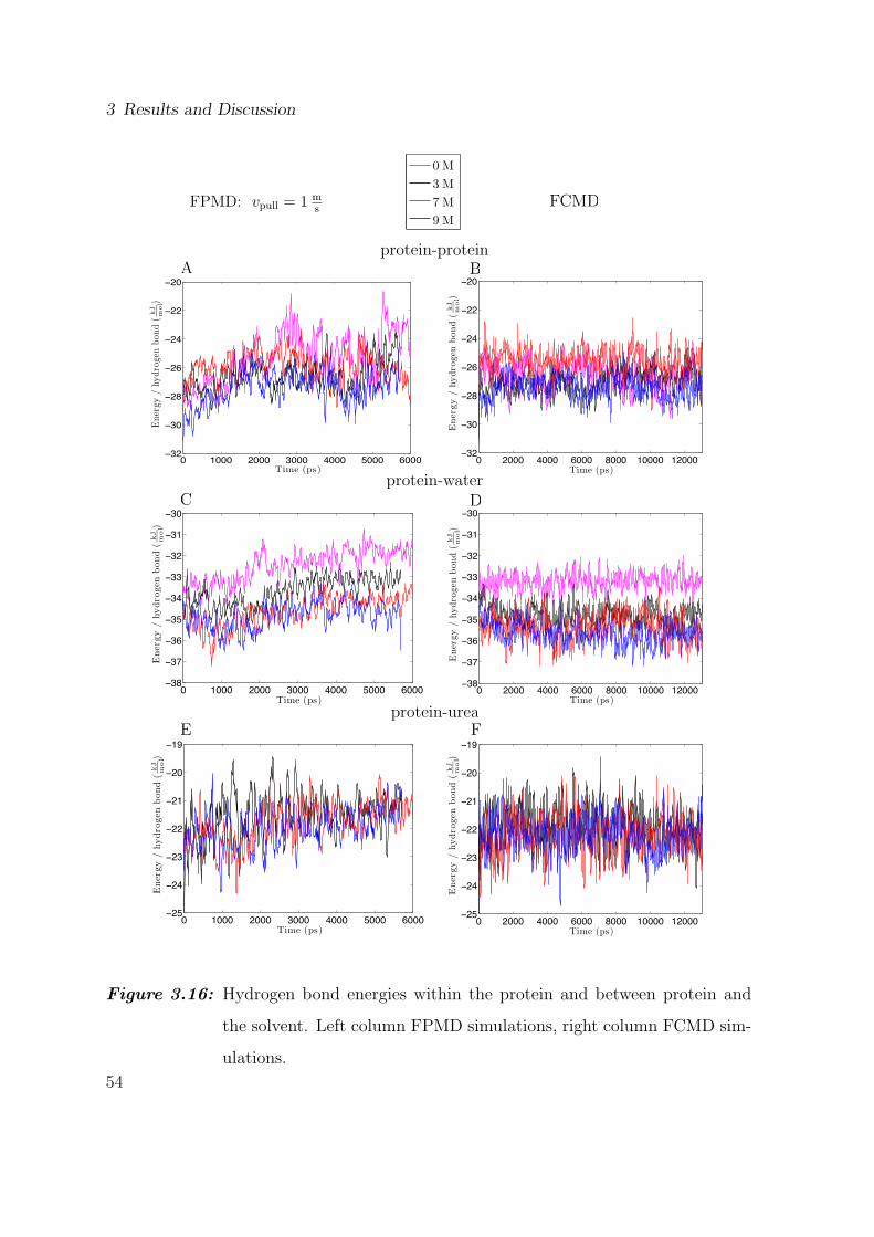
Figure 3.16: Hydrogen bond energies within the protein and between protein and
the solvent. Left column FPMD simulations, right column FCMD sim-
ulations.
54
3.5 Hydrogen Bond Energies
of hydrophobic residues to water molecules, the mean energy per hydrogen bond is
increased in respect to the initial structure. This effect provides the explanation for
the increasing energy during the unfolding process, which is however not observed in
fig. 3.16D, because the plot represents those structures, that remain in the folded state
throughout the FCMD simulation.
To complete the observation of the energy of the hydrogen bonds between the dif-
ferent components of our simulation system, we also examine the interaction between
urea and the protein. Like all the other types of interaction discussed, the values of the
hydrogen bond energy between urea and the protein are in the same order of magnitude
in the FPMD(fig. 3.16E) and FCMD(fig. 3.16F) simulations and no differences due to
a changing urea concentration arise. However, a tendency of increased energy per hy-
drogen bond in the course of unfolding is observable, because an increasing number of
less polar residues is exposed to the solvent, forming weaker hydrogen bonds. Hence
the mean energy bond increases.
The characterization of the interaction within the protein and between the protein
and the solvent by the hydrogen bond energies, reveals the influence of urea concentra-
tion. The results of the hydrogen bond energies between the protein and urea molecules
do not reveal significant differences due to a changing urea concentration. In contrast,
for both FPMD and FCMD simulations, interactions between the protein and water
show a visible effect of urea on the stability of the hydrogen bonds. Hydrogen bond
energies between protein and water are lower in the presence of urea. However, in
contrast to fig. 3.15 increasing urea concentrations did not lead to a clear gradient of
decreasing bond energies.
Two possibilities exist for an explanation of the influence of urea on unfolding of a
protein. Firstly, a direct interaction between the protein and urea might be a driving
factor for the denaturation of the protein. However, a denaturating effect of urea based
on direct interaction, as observed in [7], was not observed in our work. Secondly, urea
55
3 Results and Discussion
might affect unfolding via an indirect mechanism due to a distortion of the hydrogen
bonding pattern of water as the dominant factor for the denaturative character of
urea [8]. This distortion might lead to the increasing strenght of the hydrogen bonds
between protein and water because the water molcules may favour a bonding to the
protein instead to a bonding to urea. However, this interpretation is only speculative
and does not explain why increasing urea concentration does not further stabilize the
hydrogen bond significantly. As the values of the hydrogen bond energies between the
protein and water are nearly equal in the FPMD and FCMD simulations (fig. 3.16 C
and D, respectively), friction effects can be excluded, because they are absent in the
FCMD simulations.
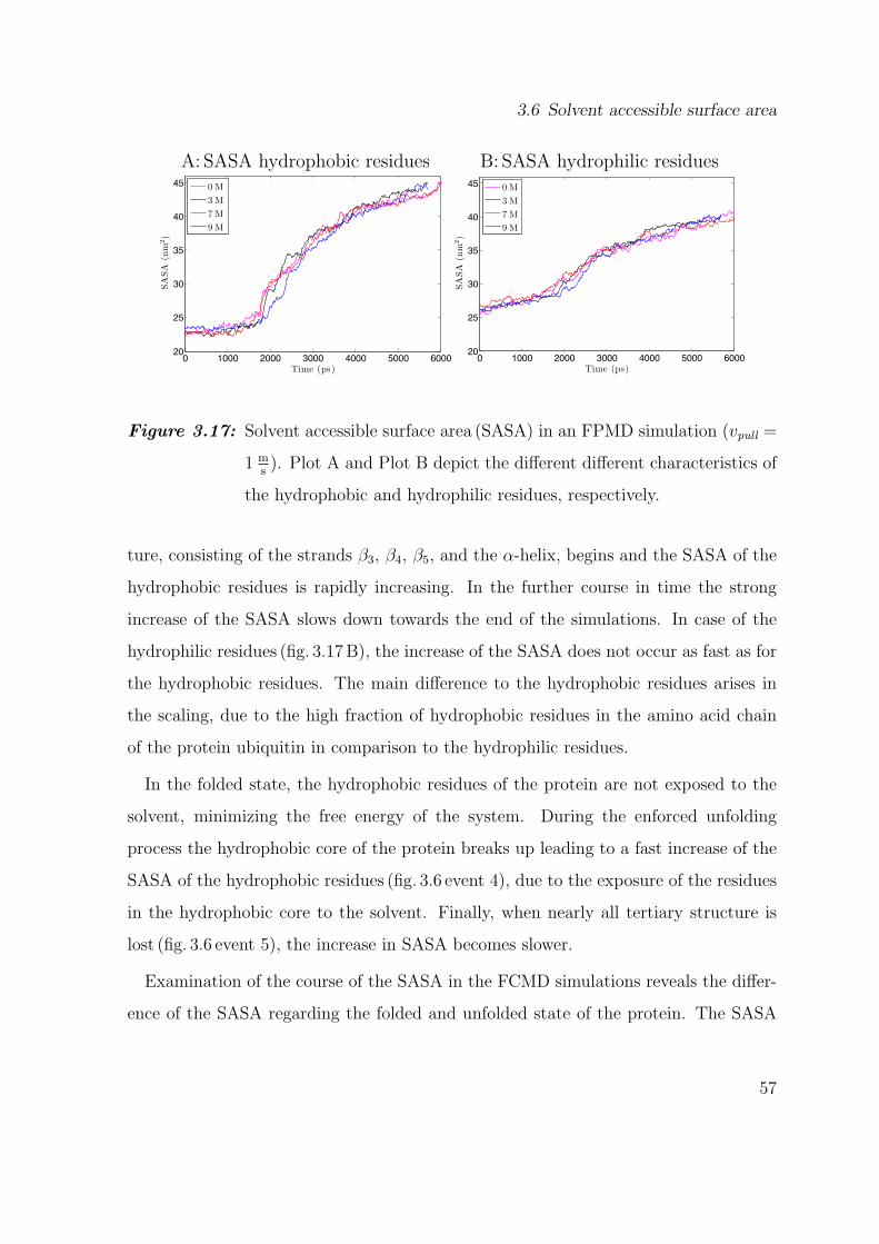
3.6 Solvent accessible surface area
Observations on the energies of the hydrogen bonds particularly yield information on
the electrostatic effect of urea on ubiquitin. Therefore the course of the solvent ac-
cessible surface area (SASA) of the residues of the protein was analyzed, to obtain
information about the influence of urea on the entropy of the system. For FPMD sim-
ulations (fig. 3.17), we averaged the results the simulations with different structures,
while in FCMD simulations no averaging was carried out because only two struc-
tures unfolded. We distinguish between the SASA of the hydrophobic and hydrophilic
residues to outline the influence of hydrophobic effects.
All FPMD simulations, independent of the pulling velocity, revealed the same charac-
teristics of the SASA in the course of the simulation. Hence we restrict the discussion
and analysis to the simulation with a pulling velocity of 1 ms. No differences in the
SASA of the hydrophobic residues (fig. 3.17A), due to a changing urea concentration
arise. In the first part of the unfolding procedure between t = 0ps and t ≈ 1800 ps
no increase is observable. At t ≈ 1800 ps the decay of the core-shaping tertiary struc-
56
3.6 Solvent accessible surface area
0 1000 2000 3000 4000 5000 600020
25
30
35
40
45
Time (ps)
SA
SA
(nm
2)
0 M
3 M
7 M
9 M
0 1000 2000 3000 4000 5000 600020
25
30
35
40
45
Time (ps)
SA
SA
(nm
2)
0 M
3 M
7 M
9 M
A: SASA hydrophobic residues B: SASA hydrophilic residues
Figure 3.17: Solvent accessible surface area (SASA) in an FPMD simulation (vpull =
1 ms). Plot A and Plot B depict the different different characteristics of
the hydrophobic and hydrophilic residues, respectively.
ture, consisting of the strands β3, β4, β5, and the α-helix, begins and the SASA of the
hydrophobic residues is rapidly increasing. In the further course in time the strong
increase of the SASA slows down towards the end of the simulations. In case of the
hydrophilic residues (fig. 3.17B), the increase of the SASA does not occur as fast as for
the hydrophobic residues. The main difference to the hydrophobic residues arises in
the scaling, due to the high fraction of hydrophobic residues in the amino acid chain
of the protein ubiquitin in comparison to the hydrophilic residues.
In the folded state, the hydrophobic residues of the protein are not exposed to the
solvent, minimizing the free energy of the system. During the enforced unfolding
process the hydrophobic core of the protein breaks up leading to a fast increase of the
SASA of the hydrophobic residues (fig. 3.6 event 4), due to the exposure of the residues
in the hydrophobic core to the solvent. Finally, when nearly all tertiary structure is
lost (fig. 3.6 event 5), the increase in SASA becomes slower.
Examination of the course of the SASA in the FCMD simulations reveals the differ-
ence of the SASA regarding the folded and unfolded state of the protein. The SASA
57
3 Results and Discussion
of the hydrophobic residues increases from 25 nm2 to about 55 nm2 in the 0M as well
as in the 7M urea solution (fig. 3.18A). However, after the complete elongation of the
protein an obvious difference arises in the further course of the SASA in the two dif-
ferent solvent environments. In case of the 7M environment, the SASA stays constant
after complete elongation, whereas in the 0M urea concentration the SASA decreases
about 5 nm2. The increase of the SASA of the hydrophilic residues (fig. 3.18B) displays
an equal character, but the increase in the SASA is only 20 nm2. As expected and sim-
ilar to the FPMD simulations, the course does not differ much from the SASA of the
hydrophobic residues.
0 2000 4000 6000 8000 10000 1200020
25
30
35
40
45
50
55
60
Time (ps)
SA
SA
(nm
2)
0 M
7 M
B: SASA hydrophilic residuesA: SASA hydrophobic residues
0 2000 4000 6000 8000 10000 1200020
25
30
35
40
45
50
55
60
Time (ps)
SA
SA
(nm
2)
0 M
7 M
Figure 3.18: Solvent accessible surface area (SASA) in the FCMD simulation, which
yielded unfolding of the protein.
The sparse results of the FCMD simulations only allow a preliminary analysis of the
influence of urea, but the characteristic decrease of the SASA in pure water after the
gained maximum indicates the influence of urea on the interaction between protein
and solvent. An explanation for the decrease is a partial refolding of the protein in
water due to the high fraction of hydrophobic residues in the amino acid chain of the
protein. Driven by the hydrophobic effect, the elongated protein attempts to minimize
its SASA in respect to the water molecules, resulting in the observed decrease of the
58
3.6 Solvent accessible surface area
SASA. The resulting slight difference in the end to end distance of the terminus Cα
atoms of the protein for the unfolded state in a 0M and 7M solution, as depicted in
fig. 3.7 effective from t ≈ 8000 ps, corroborates this explanation. In case of a 7M urea
solution it seems that the hydrophobic effect is not as pronounced allowing a larger
elongation of the protein, resulting in a larger SASA.
59
4 Summary and Conclusion
Motivated by recent simulation [1] and experimental [4, 5] studies on the protein ubiq-
uitin applying AFM methods we performed several Molecular Dynamics simulations
to explore the unfolding pathway of ubiquitin in different chemical environments. To
this end we simulated two different AFM methods enforcing the unfolding of ubiquitin.
First, we unfolded ubiquitin by pulling at the termini of the protein with potentials
moving with constant velocity (FPMD) in opposite directions. Second, the termini
were stressed with constant forces (FCMD) of 500 pN in opposite directions.
The FPMD simulations enable us to obtain an idea of the time course of the rupture
forces. However, in FPMD simulations the energy landscape of G is time dependent.
With proceeding simulation time the energy landscape G is strongly disturbed, in
contrast to FCMD simulations, in which the shift of the perturbed G remains constant
throughout a simulation. Furthermore, results from FPMD simulations are strongly
influenced by friction forces, which is not the case for FCMD simulations.
The influence of urea on the unfolding process is of interest, because urea is widely
used as denaturant, but the interaction mechanism is not clear at all [7, 8]. To elucidate
the influence of urea, four different concentrations, 0M, 3M, 7M and 9M solutions, in
the setup of the simulations were compared.
The analysis of the results of the FPMD simulations with different initial structures
revealed a very strong scattering of the rupture forces for the intial structures of the
simulations. All starting structures differ only little in the RMSD of the Cα-backbone,
60
but large differences in respect to the rupture forces in the FPMD simulations are
observable (fig. 3.4). This finding corroborates the small variance of the time course of
the forces if the same initial structures are simulated with different starting velocities
of the solvent molecules (fig. 3.3). However, although the points in time of the several
unfolding events vary as well as the corresponding rupture forces, all FPMD simulations
even when performed with different structures, equal in respect to the order of rupture
events, independent of the urea concentration.
The influence of urea on the velocity of the loss of the secondary structure motifs is
somewhat unexpected; no direct relation between rupture forces and increasing urea
concentration is observable. However, the presence of some urea molecules (3M) seems
to stabilize the protein, though it is actually know for its denaturant characteristics.
Yet in both cases the expected influence of urea might simply be hidden by the large
scatter of the forces.
The extremely high forces in combination with only a slight increase with the chang-
ing of the pulling velocities from 1 ms
to 10 ms
reflects that the simulated system is
strongly influenced by friction effects of the solvent during the unfolding process [33].
To analyse whether the unexpected influence of urea is an artefact, due to high fric-
tion occuring in FPMD simulations, we try to extrapolate the rupture force to the low
friction regime. However, a reliable fit of the forces to the model resulting in eq. 2.18
and hence extrapolation to the low friction regime, governing AFM experiments is im-
possible due to the strong variance of the different simulations. Assuming a strong
influence of hydrodynamic effects a speculative explanation for the absence of the de-
naturative effects of urea is possible. An increasing urea concentration leads to a non
linear increase of the viscosity of the solvent [33], which might outbalance the denat-
urative effects of urea in a pulling simulation. However, at high urea concentrations,
more urea molecules aggregate at the surface of the protein and may affect it in a
denaturative way, such that the rupture forces decrease despite an increasing viscosity
61
4 Summary and Conclusion
of the solvent. But also in this case the effect could simply have a statistical character.
Furthermore, the strongly differing force profiles of the different starting structures
corroborate that quantitative conclusions about the course of Gibb’s free energy during
unfolding are infeasible. A possible explanation might arise from a strong deformation
of the Gibb’s free energy landscape, due to the fast pulling. The possibility to over-
come the energetic barriers for an unfolding event is strongly increased resulting in the
differing points in time and forces for the unfolding events (fig. 3.4).
A different unfolding pathway of ubiquitin found in the FCMD simulations, compared
to the FPMD simulations, reflects the influence of the two methods to apply a force
on the termini of the protein on the Gibb’s free energy landscape. Here, only two
simulations yield an unfolding event and conclusions are only speculative. However,
the observed unfolding events might reflect the denaturative character of urea in respect
to the secondary structure of the protein. The unfolding of the protein in a solution
containing urea starts much earlier than the observed unfolding event in pure water.
Furthermore, the FCMD simulation in urea leading to unfolding of ubiquitin shows a
larger elongation of the protein in comparison to the unfolding in pure water. These two
effects might support our interpretation for the unexpected behaviour of the protein in
the different urea solutions in the FPMD simulations, because in the FCMD simulations
friction and hydrodynamic effects do not play a decisive role until the main unfolding
event starts. In 7M urea concentration the elongation proceeds with a velocity of
several ms. Hence the longer unfolding time of the structure in a 7M urea solution in
comparison to pure water might point to a possible influence of the viscosity of the
solvent. However this effect could also depend on the mechanical stress and once again
the statistics of the simulated process are too bad for a reliable conclusion.
The results of the energetic environment of the protein in terms of hydrogen bond en-
ergies and the solvent accessible surface area of the protein do not allow a clear conclu-
sion about the interaction mechanism between urea, the protein, and water molecules.
62
As proposed by one model of the urea-water interaction [8] low urea concentrations
strongly disturb the hydrogen bonding pattern of water, yielding a decrease in the
solvent entropy, an effect that indirectly affects the stability of the protein. However,
current MD studies on urea [7] suggest, that urea directly affects the protein. Our
results show a stabilization of the bonds between protein and water in the presence of
urea. With increasing urea concentration more urea molecules may replace the weak
hydrogen bonds between water and the less polar residues. Hence, the average energy
of the hydrogen bonds decreases. However, this effect decreases with increasing urea
concentration, because most less polar residues are saturated already at low urea con-
centrations. This interpretation points again to a direct interaction mechanism of urea
and the protein.
In summary, our studies show the high dynamics of the protein ubiquitin and a
complex interaction of the protein with urea. The denaturative character of urea is
not observed in the simulations, particularly low urea concentrations seem to have a
stabilizing effect on the protein (high rupture force), but this effect might be explained
with the help of the friction between the protein and the solvent due to fast pulling.
Hence, an improved insight into the interaction mechanism between the solvent and
the protein could be gained by much slower FPMD simulations, which minimize the
hydrodynamic effects and elucidate the influence of urea on the Gibb’s free energy
landscape of the protein ubiquitin. Additional FCMD simulations, which last more
than 20 ns or application of a higher force on the protein, could provide more unfold-
ing events providing a possibility to refine the information on the energy landscape.
Definitely many simulations with different starting structures have to be performed to
get a deeper insight into the statistics of the unfolding process in the various chemical
environments.
63
Acknowledgements
Very many thanks to Prof. Dr. Hermann Gaub and Prof. Dr. Helmut Grubmuller
for providing me the possibility to join Mr. Grubmullers group at the department of
Theoretical and Computational Biophysics of the Max-Planck Institute for Biophysical
Chemistry in Gottingen and their continuous support in every aspect of this work.
Thanks to all group members for their patience, when the cluster nodes were filled
up with my simulation jobs. Special thanks to Frauke Grater and Wolfram Stacklies
for providing parts of the source code for the FCMD simulations. Furthermore special
thanks to Ira Tremmel and Martin Stumpe for very generative discussions on this work.
Additionally many thanks to my family, which supported me in all unscientific aspects
during my whole studies. Finally I would like to thank my physics teacher Mr. Kuhnel,
for his encouraged school, that sparked my interest, resulting in the physics studies.
64
Bibliography
[1] Frauke Grater and Helmut Grubmuller. Fluctuations of primary ubiquitin folding
intermediates in a force clamp. Journal of Structural Biology, 157:557–569, 2007.
[2] W. F. van Gunsteren and H. J. C. Berendsen. Computer simulation of molecular
dynamics: Methodology, application, and perspectives in chemistry. Angewandte
Chemie, 29:992–1023, 1990.
[3] W. F. van Gunsteren et. al. Biomolecular modeling: Goals, problems, perspectives.
Angewandte Chemie, 45:4064–4092, 2006.
[4] Michael Schlierf, Hongbin Li, and Julio M. Fernandez. The unfolding kinetics of
ubiquitin captured with single molecule force clamp techniques. Proceedings of the
National Academy of Sciences of the United States of America, 101(19):7299–7304,
May 2004.
[5] Julio M. Fernandez and Hongbin Li. Force-clamp spectroscopy monitors the fold-
ing trajectory of a single protein. Science, 303:1674–1678, March 2004.
[6] Julia Wirmer, Wolfgang Peti, and Harald Schwalbe. Motional properties of un-
folded ubiquitin: a model for a random coil protein. Journal of Biomolecular
NMR, 35:175–186, 2006.
[7] Martin C. Stumpe and Helmut Grubmuller. Aqueous urea solutions: Structure,
65
Bibliography
energetics and urea aggregation. Journal of Chemical Physics B, 111:6220–6228,
2007.
[8] A. Idrissi. Molecular structure and dynamics of liquids: aqueous urea solutions.
Spectrochimica Acta Part A, 61:1–17, 2005.
[9] Sequence details of ubiquitin 1UBQ. http://www.pdb.org.