The University of Texas at Austin Marine Science Institute P.o. Box 1267 Port Aransas, Texas 78373-1267

PREDICTING LONG-TERM EFFECTS OF FRESHWATER INFLOW ON MACROBENTHOS IN

THE LAVACA-COLORADO AND GUADALUPE ESTUARIES

Paul A. Montagna, Principal Investigator

TWDB Contract No. 91-483-787

Technical Report Number TR/91-004

FINAL REPORT

PREDICTING LONG-TERM EFFECTS OF FRESHWATER INFLOW

ON MACROBENTHOS IN THE

LAVACA-COLORADO AND GUADALUPE ESTUARIES

by

Paul A. Montagna, Principal Investigator

from

University of Texas at Austin

Marine Science Institute

P.O. Box 1267

Port Aransas, Texas 78373

to

Texas Water Development Board

P.O. Box 13087 Capitol Station

Austin, Texas 78711

Interagency Cooperative Contract

TWDB Contract No. 91-483-787

The University of Texas Marine Science Institute Technical Report Number

TR/91-004

October 1991

PREDICTING LONG-TERM EFFECTS OF FRESHWATER INFLOW ON

MACROBENTHOS IN THE LAVACA-COLORADO AND GUADALUPE ESTUARIES

TABLE OF CONTENTS

ABSTRACT................................................... 1

INTRODUCTION 1

METHODS................................................... 2

Why Study Benthos? ....................................... 2

Study Design and Area ..................................... 2 Hydrographic Measurements ................................. 6

Geological Measurements ................................... 7

Chemical Measurements 7

Biological Measurements .................................... 7

Statistical Analyses ........................................ 8

RESULTS. . . . . . . . . . . . . . . . . . . . . . . . . . . . . . . . . . . . . . . . . . . . . . . . . . . . 9

Guadalupe Estuary ........................................ 9

Lavaca-Colorado Estuary . . . . . . . . . . . . . . . . . . . . . . . . . . . . . . . . . . .. 23

Lavaca-Colorado Estuary Station A . . . . . . . . . . . . . . . . . . . . . . . . . . . .. 24

DISCUSSION ................................................. 39

CONCLUSION ................................................ 41

ACKNOWLEDGEMENTS ......................................... 42

REFERENCES ................................................ 42

EFFECTS OF THE LAGUNA MADRE, TEXAS BROWN TIDE ON BENTHOS

............................................................ 68

The Brown Tide Event . . . . . . . . . . . . . . . . . . . . . . . . . . . . . . . . . . . . .. 68

The Effect of Brown Tide on Benthos ........................... 69

PREDICTING LONG-TERM EFFECTS OF FRESHWATER INFLOW ON

MACROBENTHOS IN THE LAVACA-COLORADO AND GUADALUPE ESTUARIES

ABSTRACT

Two estuaries have been studied to determine the effect of year-to-year variation

of freshwater inflow on macrobenthic infauna. The estuaries have similar inflow

characteristics, but the Lavaca-Colorado has direct exchange of coastal marine water with

the Gulf of Mexico and the Guadalupe does not. Studies in the Lavaca-Colorado began

in 1984, and studies in the Guadalupe began in 1987. There are changes in community

structure and function from year-to-year, which can be linked to the long-term cycle of wet and dry years along the Texas coast. There appears to be a long-term cycle of high­

inflow stimulated recruitment, followed by nutrient depletion and recruitment of marine

species during low-inflow periods, followed by declines in productivity until the next wet

year. These cycles appear to have a period of 2-3 years, but it will take at least 3 more

years of data to test this hypothesis.

INTRODUCTION

Prudent management of freshwater resources is required to meet residential, industrial, and agricultural needs while still protecting the natural resources in our

environment. One aspect of environmental conservation (as evidenced by good

management practices) is to ensure that there is adequate freshwater inflow to our

estuaries. Data is needed to describe the effects of freshwater inflow on estuaries, so that

an assessment of freshwater needs can be made.

The climate of Texas is characterized by a long-term cycle of floods and droughts.

Yet, we have very little information about the scales of natural variability over the long­

term. This makes it very difficult to create long-range plans for the management of water resources. Data is needed to describe the long-term variability of biological indicators of

freshwater inflow effects.

Previous studies have shown that benthos are good indicators of freshwater inflow

effects (Montagna, 1989; Kalke and Montagna, 1991; Montagna and Yoon, 1991; Montagna and Kalke, submitted ms.). However, all of these studies were carried out over

a narrow time scale, from seven to 21 months. The studies spanning more than one year

hint that there is a long-term effect associated with wet and dry years. The purpose of

1

this study is to determine if freshwater inflow affects on benthos is greater for year -to-year variability than for seasonal variability. This would allow us to build better models of quantitative relationships between freshwater inflow and benthos in Texas estuaries.

METHODS

Why Study Benthos?

Benthos are the most economical and reliable indicators of the effects of freshwater inflow in Texas estuaries. This contradicts the conventional wisdom. Rivers transport

nutrients to estuaries, which should stimulate phYtoplankton production (Nixon et aI.,

1986). The benthos would benefit by this production if filter feeders, e.g., oysters consume phytoplankton in the water column or if the primary production is deposited to the bottom via gravity. Previous studies have shown that phytoplankton parameters are

very variable. Primary production can vary as much over one or two days as it can over

a week. Therefore, we have not been successful in correlating primary production with

river inflow. We also don't know what taxonomic groups, let alone species, are

responding to the inflow. It would be very labor intensive and expensive to generate

enough data to fully describe the natural variability in primary production and

phytoplankton species distributions to determine if man's activities in managing freshwater inflow would increase that variability. Benthos, on the other hand, are relatively fixed in space and easy to sample accurately, long-lived and integrate effects over a long time

period, and many community characteristics can be measured inexpensively.

Study Design and Area

There are seven major estuarine systems along the Texas coast (Figure 1). Each

system receives drainage from one to three major rivers. The northeastern most

estuaries receive more freshwater inflow than the southwestern estuaries (Figure 2). Two estuarine systems were studied in detail (Figure 3). Both systems have similar freshwater

inflow characteristics, but the Lavaca-Colorado has direct exchange of marine water with

the Gulf of Mexico via Pass Cavallo, whereas the Guadalupe does not. To assess

ecosystem-wide variability stations in the freshwater influenced and marine influenced

zones were chosen. Two stations, which replicate each of the two treatment effects

(freshwater and marine) influence, were sampled. Generally these stations were along

the major axis of the estuarine system leading from river mouth to the foot of the estuary

2

I 1 "~N£OY

I L_ I 'l'l'lll.&~Y -, .

I-w-.../""'

TEXAS \ " ~ /"". CA.IoII(AON

£c$I Atfclt2gDrdD ,sIt/Dry

CC/DrtldD ,sIt/Dry

LDflDca-Trl!s Pa/(Jc;os ,slt/ary

...

Miss;on-Arans(ls lI$1ua,J'

Laguna Modr/! I!sluory

o 10 Ie 50 .0 "ll£S =r= T-=-:J

o I.... )0 .~ 601(IlO ... (T(RS ~:"J;-~

Figure 1. Location of Texas Estuaries.

3

47 - year (1941-1987) Average Freshwater Inflow Balance (109 acre - ft . y)

Inflow 14 ,-------------------------------,

13 x

12 l>)'> 1>/> »)<

11

-1 ~----------------------------~

SN TJ LC GE MA NC LM

Estuary

Figure 2. Annual average inflow in Texas Estuaries. SN=Sabine-Neches, TJ=Trinity­

San Jacinto, LC=Lavaca-Colorado, GE=Guadalupe, MA=Mission-Aransas, NC=Nueces, LM=Laguna Madre (doesn't show at this scale).

4

..

" Guadalupe

:"::""": River

.. '. ', .....

.. ', .

San Antonio Bay

, .... . :. Tres Palacios

River

Figure 3. Sampling locations within the Guadalupe and Lavaca-Colorado Estuaries.

5

near the barrier island. This design avoids pseudoreplication, where only one station has

the characteristic of the main effect, and it is not possible to distinguish between station

differences and treatment differences.

The Lavaca River empties into Lavaca Bay, which is connected to Matagorda Bay.

Matagorda Bay also has freshwater input from the Colorado and Tres Palacios River.

Over a 47-year period (1941-1987) the Lavaca-Colorado Estuary received an average of

3.800x109 m3 y-1 with a standard deviation of 2.080 m3 y.1 (3.080 ± 1.686 x106 ac-ft y-1)

of freshwater input, and the freshwater balance (input-output) was 3.392x109 m3 y-1 with

a standard deviation of 2.345x109 m3 y.1 (2.750 ± 1.901 x106 ac-ft y-1) (TDWR, 1980a;

TWDB unpublished data). Four Stations were occupied along the axis of the system.

Two stations were in Lavaca Bay (A and B), and two stations were in Matagorda Bay (C

and D) (Figure 3). Depths of stations A, B, C, and D were 1.3 m, 2.0 m, 3.1 m, and 4.2

m, respectively. Five field trips were performed. Station A in Lavaca Bay was the same

station 85 sampled in 1984-1986 (Jones et aI., 1986).

The San Antonio River joins the Guadalupe River that flows into San Antonio Bay.

Over a 46-year period the Guadalupe Estuary received an average of 2.896x109 m3 y.1

with a standard deviation of 1.597 m3 y-1 (2.347 ± 1.295 x1 06 ac-ft y.1) of freshwater input,

and the freshwater balance (input-output) was 2.624x109 m3 y.1 with a standard deviation

of 1.722x1 09 m3 y-1 (2.127 ± 1.396 x106 ac-ft y.1) (TDWR, 1980b; TWDB unpublished

data). This system was studied from January through July 1987. Four stations were

occupied: freshwater influenced stations at the head of the bay (station A) and at mid-bay

(station B), and two marine influenced stations near the Intracoastal Waterway, one at the

southwestern foot of the bay (station C) and one at the southeastern foot of the bay

(station D) (Fig. 1). Stations were sampled five times in the first year. All stations were

in shallow water. Depths of stations A, B, C, and D were 1.3 m, 1.9 m, 2.0 m, and 1.6

m, respectively.

Hydrographic Measurements

Salinity, conductivity, temperature, pH, dissolved oxygen, and redox potential were

measured at the surface and bottom at each station during each sampling trip.

Measurements were made by lowering a probe made by Hydrolab Instruments. Salinities

levels are automatically corrected to 25°C. The manufacturer states that the accuracy

of salinity measurements are 0.1 ppt. When the Hydrolab instrument was not working,

water samples were collected from just beneath the surface and from the bottom in jars,

and refractometer readings were made at the surface.

6

Geological Measurements

Sediment grain size analysis was also performed. Sediment core samples were

taken by diver and sectioned at depth intervals 0-3 cm and 3-10 cm. Analysis followed

standard geologic procedures (Folk, 1964; E. W. Behrens, personal communication).

Percent contribution by weight was measured for four components: rubble (e.g. shell

hash), sand, silt, and clay. A 20 cm3 sediment sample was mixed with 50 ml of hydrogen

peroxide and 75 ml of deionized water to digest organic material in the sample. The

sample was wet sieved through a 62 JIm mesh stainless steel screen using a vacuum

pump and a Millipore Hydrosol SST filter holder to separate rubble and sand from silt and

clay. After drying, the rubble and sand were separated on a 125 JIm screen. The silt and

clay fractions were measured using pipette analysis.

Chemical Measurements

The vertical distribution of carbon and nitrogen content of sediments was measured

in October 1990. One m cores were sectioned every 10 cm. Two replicate cores were

taken at each station. The samples were frozen until they were prepared for analysis.

Sediments were prepared for analysis of total carbon and nitrogen by drying at 50 'C for

24 h, after which they were ground into a fine powder with a mortar and pestle. A Perkin­

Elmer 240B elemental analyzer was used for sample analysis. Sample sizes of about 120

mg for sediments were necessary for adequate detection of carbon.

Quality control was determined by running a blank, and standards at the beginning

and ending of each days measurements. Blank values were used to determine the

validity of the days runs. If blanks were too high, then the data were rejected. Caffeine

was used as the standard. Over all runs, the average measured carbon value was

50.98% (± 2.14 SD), and the average nitrogen value was 31.23% (± 1.22). Indicating the

precision for replicate measurements (Le., the coefficient of variation) was ± 4.2% for

carbon and ± 3.9% for nitrogen. The true values are 49.48% for carbon and 28.85% for

nitrogen. Indicating the accuracy (calculated as 100x[observed-true]jtrue) was ± 3.3%

for carbon and ± 8.2% for nitrogen.

Biological Measurements

Sediment was sampled with core tubes held by divers. The macrofauna were

sampled with a tube 6.7 cm in diameter, and sectioned at depth intervals of 0-3 cm and

3-10 cm. Three replicates were taken within a 2 m radius. Samples were preserved with

7

5% buffered formalin, sieved on 0.5 mm mesh screens, sorted, identified, and counted.

Each macrofauna sample was also used to measure biomass. Individuals were combined into higher taxa categories, Le., Crustacea, Mollusca, Polychaeta, Ophiuroidea, and all other taxa were placed together in one remaining sample. Samples were dried for 24 h at 55 ·C, and weighed. Before drying, mollusks were placed in 1 N HCI for 1

min to 8 h to dissolve the carbonate shells, and washed with fresh water.

Statistical Analyses

Statistical analyses to reveal differences among cruises, stations and sediment

depths were performed using general linear model procedures (SAS, 1985). Two-way

analysis of variance (AN OVA) models were used where sampling dates and stations were the two main effects. Tukey multiple comparison procedures were used to find a

posteriori differences among sample means (Kirk, 1982). Multivariate ANOVA was used to test for treatment effects on species data. Factor analysis and cluster analysis was

used to determine if communities were similar on different sampling dates. Linear

correlation coefficients were calculated to determine if salinity was correlated to

macrofauna abundance, biomass or diversity. Diversity is calculated using Hill's diversity

number one (N1) (Hill, 1973). It is a measure of the effective number of species in a

sample, and indicates the number of abundant species. It is calculated as the

exponentiated form of the Shannon diversity index: N1 = eH' (1)

The Shannon index is the average uncertainty per species in an infinite community made

up of species with known proportional abundances (Shannon and Weaver, 1949). The

Shannon index is calculated by:

(2)

Where n1 is the number of individuals belonging to the ith of S species in the sample and

n is the total number of individuals in the sample.

8

RESULTS

There is a linear decrease in average annual freshwater inflow from north to south

along the Texas coast (one-way ANOVA, P = 0.0001, Figure 2). The Lavaca-Colorado

and Guadalupe Estuaries have the same average inflow (linear contrast, P = 0.3333,

Figure 2). Lavaca-Colorado and Guadalupe Estuaries are very different in certain respects. The Lavaca-Colorado is much larger, receives drainage from three rivers, has a typical primary and secondary bay configuration, and has excellent exchange with the

Gulf of Mexico (Figure 3). The Guadalupe has restricted Gulf exchange and is composed

of a single bay. The impact of human activities is very different also. The Guadalupe receives drainage from the San Antonio River, which passes through a major metropolitan

area, yet San Antonio Bay is very rural. The Lavaca-Colorado watershed is mostly rural,

but Lavaca Bay is heavily impacted by channels, ship traffic, and the chemical industry.

I must use salinity as an indicator of freshwater inflow. Assessments of freshwater inflow into the Guadalupe and Lavaca-Colorado do not extend beyond 1988.

Guadalupe Estuary

Since 1987, the Guadalupe has gone through three different phases (Figure 4,

Table 1). There was a great flood in the spring of 1987. In the summer of 1987, even

the stations located in the zone of greatest marine influence had salinities of near zero.

A two year drought followed that period. During the drought salinities rose to 20-30 ppt throughout the estuary. The period since April 1990 has been one of fluctuations.

Salinities in the upper part of the estuary dropped to near zero during spring floods, but

the salinities at the lower end of the estuary, only dropped to the 6-12 range. The period

during the spring of 1991 looks a lot like the period prior to the flood of the spring of 1987.

The sediments of the upper part of the estuary are characterized by high silt and

clay contents (Figure 5, Table 2). Only station D sediments were dominated by sand.

Rubble was common in deep sediments from A, and shallow sediments in C. Correlated with the high sand content, station D had the lowest carbon (Figure 6) and nitrogen

(Figure 7) contents of all stations (Table 3). There was considerably more carbon

throughout the top m of sediment in stations A and B than in C and D. Nitrogen content

was higher in A and B only in the top 40 cm.

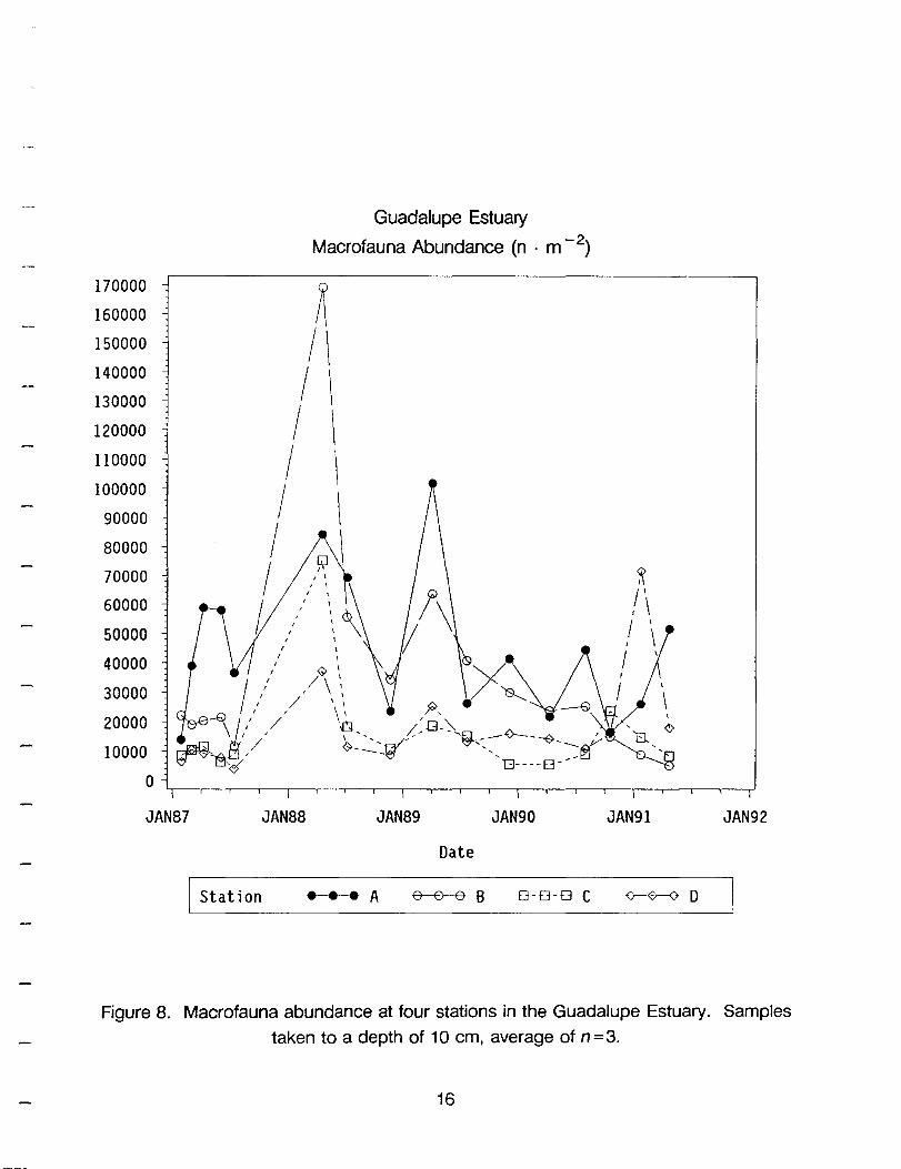
Macrofauna abundance (Figure 8) and biomass (Figure 9) are generally higher in stations A and B in the upper end of the estuary than in stations C and D in the lower end

of the estuary (linear contrast, P=0.0001 for both). The average density (in units of

9

individuals· m-2) over the entire study period was 44,512 at A, 35,318 at B, 17,474 at D,

and 15,629 at C (Table 4). The average biomass (in units of g • m-2) during the entire

study period was 9.47 at A, 6.95 at B, 5.41 at D and 3.06 at C. An exception to the

generality is biomass in station D when rare, but large, ophiuroids are present (Figure 9).

There were large year-to-year fluctuations in both parameters during the course of the

study, but in general, the station pairs changed in similar ways.

Average estuarine-wide salinity was plotted with average estuarine-wide abundance

(Figure 10), average estuarine-wide biomass (Figure 11), and average estuarine-wide

diversity (Figure 12) to determine the relationship between freshwater inflow and biological

response. Over time, biomass was significantly correlated with changes in salinity

(r=0.59, P=0.0164), but abundance was not (r=0.32, P=0.2277). However, simple

correlation does not explain the response completely. The highest abundance, over

90,000.m·2, occurred in 1988, following the flood of 1987. Density dropped with

sustained high salinities during 1989 and 1990. Biomass also increased to peak levels

after the flood of 1987, and was declining during the drought of 1989-1990. Together,

these data suggest that periodic flooding, and resulting nutrient enrichment are required

to maintain a productive benthic ecosystem. Hill's diversity index was highly correlated

with salinity (r=0.71, P =0.0020). Diversity is most affected when there are floods. During

floods diversity drops to very low levels. The lower diversity is probably resulting from

displacement of marine species with freshwater species. There are fewer species present

in the upper reaches of the estuary than in the lower reaches (Table 5). There appears

to be a succession of species groups through time. The first two factors in a factor

analysis of sampling dates accounts for 77% of the variability in the species dataset. The

first factor appears to be related to suites of freshwater species since the dates during the

flood of 1987 are separated from other groups along that axis (Figure 13). Marine

conditions prevailed from July 1988 to July 1989 and these dates separate along the axis

of the second factor, indicating the second factor is related to a suite of marine species.

January 1987 also separates as a marine period. Transitional periods are in the center

of the factor analysis. A cluster analysis shows a similar trend (Figure 14). In the cluster

analysis dates from March 1987 to December 1989 separate from later dates, suggesting

that succession to marine conditions were complete to that date. January 1987 separates

out with the latter dates, since marine conditions prevailed prior to the 1987 flood.

10

p P

40

30

Guadalupe Estuary Salinity (ppt)

t 20

10

o ~~~~~~~~~~~~~~~~--~r-r-~ JAN87 JAN88 JAN89 JAN90 JAN91 JAN92

Date

I Station • • • A e----B----B B 0 - 0 - 0 C ()--~ D

Figure 4. Bottom water salinity at four stations in the Guadalupe Estuary.

11

Figure 5. Sediment grain size in the Guadalupe Estuary. Samples taken in October

1990. STASEC = Station, vertical section combination. Section in cm.

12

Guadalupe Estuary Sediment Composition (% dry weight)

STASEC=A 0-3

CLAY

SAND ?-=:::::::::::=l-- RUBBLE

'--~- SILT

STASEC=B 0-3

CLAY

RUBBLE SAND -~ SILT

STASEC=C 0-3

RUBBLE CLAY

SAND

SILT

STASEC=D 0-3

SAND ~===!--- RUBBLE SILT

13

RUBBLE

SAND

CLAY

RUBBLE SAND

SAND

SAND

STASEC=A 3-10

CLAY

SILT

STASEC=B 3-10

'----- SILT

STASEC=C 3-10

,----- CLAY

r=:::::::::::l-- RU BB L E

'---SILT

STASEC=D 3-10

CLAY

RUBBLE SILT

dm o

-1

-2

-3

-4

-5

-6

-7

-8

-9

-10

o

« I , r ,

J \ ,

1> ,

J I ,

1>

I <l>

I ,

I Station

<) , /

1

Guadalupe Estuary Total Carbon (% dry weight)

2

c

, Q , ,

, , ~ , I I

4J , , ,

, ,

3

, [l

• •• A e-e-e B 0-0-0 C

4 5

Figure 6. Vertical distribution of carbon in sediments from the Guadalupe Estuary.

Samples taken October 1990 at 10 cm intervals, average of n=2, 1 dm=10 cm.

14

dm 0

<;> , COL

-1 \ , 1>

-2 / ~

-3 \

-4 \ ~

-5 /

i -6 / ,

f -7

, I ,

-8 I , I .c{ , ~

-9 I ~

~

~

, [~(

-10

0.01 0.02 0.03

I Station

,Cl

Guadalupe Estuary Total Nitrogen (% dry weight)

/ /

'Et 0-...... _____

----- -----'iiJ , , ----, ----0 ~----,

/ ~

/ -_/---~

\ /

~

I ~

0.04 0.05 0.06 0.07 0.08 0.09

N

---------~

0.10 0.11

• • • A e--B--e B 0-0-0 C 0-0-0 D

Figure 7. Vertical distribution of nitrogen in sediments from the Guadalupe Estuary.

Samples taken in October 1990 at 10 cm intervals. 1 dm = 10 cm.

15

170000

160000

150000

140000

130000

120000

110000

100000

90000

80000

70000

60000

50000

40000

30000

20000

10000

o JAN87

I Stat ion

JAN88

Guadalupe Estuary

Macrofauna Abundance (n . m -2)

JAN89 JAN90

Date

0-0-0 C

JAN91 JAN92

Figure 8. Macrofauna abundance at four stations in the Guadalupe Estuary. Samples

taken to a depth of 10 cm, average of n=3.

16

Biomass 40

30

20

10

o JAN87

I Station

JAN88

Guadalupe Estuary

Macrofauna Biomass (g . m -2)

1\ <;>

/ \ /\ , ' / \

\ , \

\ ,

JAN89 JAN90

Date

0-0-[3 C

JAN91 JAN92

<:t--0---<) D

Figure 9. Macrofauna biomass at four stations in the Guadalupe Estuary. Samples

taken to a depth of 10 cm, average of n=3.

17

Guadalupe Estuary

Macrofauna Abundance (n . m -2) and Salinity (ppt)

Abundance 100000 f- 30

90000 II 80000 - I I ,~ , ,0 ,

)3-" , , 'Q ,

1 ,I: ,

70000 'tf , £J , " ,

1 el\ Q [if , ,

I ,

, ,

,., \ ,

60000 I , I , I I , I

/..:1

I , I I

I I

l I ,

50000 I I I I

I: I 1 \

I I

,/ ~ I I

40000 I I I ' I'

, I

~,I/ \ 1 I' I

\ I' I [CJ ,

30000

if:A 1/ \ 1 !\ ~ J'J ~--B I "

20000 ' j' ~ ~ /~ ~ 7 ~/ V

10000 -I I I I I , I

JAN87 JAN88 JAN89 JAN90 JAN91 JAN92

Oate

Figure 10. Relationships between macrofauna abundance (0) and salinity (0) in the

Guadalupe Estuary. Average abundance and salinity at all stations.

18

20

10

0

s a 1

n i t Y

Biomass 14

13

12

11

10 -

9 -

8 -

7

6

5

4

3

Guadalupe Estuary

Macrofauna Biomass (g . m -2) and Salinity (ppt)

, , , , , ,

, ,

30

20 S

10

o

a 1 i n i t Y

JAN87 JAN92

Date

Figure 11. Relationships between macrofauna biomass (0) and salinity (0) in the

Guadalupe Estuary. Average biomass and salinity at all stations.

19

Guadalupe Estuary Macrofauna Diversity (Hill's N1) and Salinity (ppt)

Diversity 70

.---________________________ ~ Sal inity 30

60

20

30 - 10

20

\ , \ I , I

\ I

[']

10 -l __ ~_.~,_._~_.~,_._~_.~,_._~_.-,_._~_,-,_~ T ' I' I' I' I I

JAN87 JAN88 JAN89 JAN90 JAN91 JAN92

Date

Figure 12. Relationships between macrofauna diversity (0) and salinity (0) in the

Guadalupe Estuary. Average diversity and salinity at all stations.

20

o

Figure 13. Factor analysis for macrofauna species at all sampling dates in the

Guadalupe Estuary. Species occurring at all stations for a given date.

Guadalupe Estuary Principal Factor Analysis With PROMAX Rotation

Factor 1 1.0

JUL87 ..l N87

0.8

APR87

0.6 MAA87

0.4

0.2 - ceca

APR88 JUlB9 N0V8S AlJG90 PR90 JUl88

0.0 APR89 JAN87

-0.2 JAN91

-0.4

-0.6

-0.8

-1.0 I I I I I I I I I

-1.0 -0.8 -0.6 -0.4 -0.2 0.0 0.2 0.4 0.6 0.8

Factor 2

21

I

1.0

DISTANCE METRIC IS EUCLIDEAN DISTANCE SINGLE LINKAGE METHOD (NEAREST NEIGHBOR)

TREE DIAGRAM

0.000 JAN87

APR89

JUL89

APR87

JUN87

MAR87

JUL88

NOV88

JUL87

APR88

DEC89

AUG90

OCT90

APR90

JAN91

APR91

-

-

-

-

}

DISTANCES 50.000

r--

.

r-

r-

r-

Figure 14. Cluster analysis of sampling dates for Guadalupe Estuary. Distance metric

is euclidean distance single, linkage method (nearest neighbor)

22

Lavaca-Colorado Estuary

Station A was also studied during 1984-1986, and called station 85 in previous

studies (Kalke and Montagna, 1991). Unfortunately, my record is incomplete during 1987,

so we can not look at the effect of the spring flood in the Lavaca-Colorado Estuary (Table

6). However, the period between 1984 and 1985 was a very wet period indicated by low

salinities in station A (Figure 15). 1986 to early 1987 was dry, and similar to the recent

period from April 1990 to the present. 1988 through 1989 was the highest salinity period

recorded.

The sediments of the upper part of the estuary are characterized by high silt and

clay contents (Figure 16, Table 2). Station C sediments were dominated by rubble and

sand. Sand, silt and clay are equally abundant at station D. Rubble was common in

sediments from C. Correlated with the high sand content, station D had the lowest

carbon (Figure 17) and nitrogen (Figure 18) contents of all stations (Table 3). The

patterns of carbon content throughout the top m of sediment were different in the two

parts of the estuary. Carbon was higher in the top 30 cm at stations C and D, but

relatively uniform through the to m of sediment at stations A and B. Nitrogen content was

higher in A and 8 than in C and D, but only in the top 50 cm.

Macrofauna abundance (Figure 19) and biomass (Figure 20) are generally higher

in stations C and D in the lower end of the estuary than in stations A and 8 in the upper

end of the estuary (linear contrast, P=0.0001 for both). The average density (in units of

individuals· m·2) over the entire study period was 10,347 at A, 10,012 at 8,20,909 at D,

and 30,689 at C (Table 7). The average biomass (in units of g • m-2) during the entire

study period was 2.42 at A, 3.47 at 8, 12.71 at C, and 19.22 at D. There were large year­

to-year fluctuations in both parameters during the course of the study, but in general, the

station pairs were changed in similar ways. There were more polychaete and crustacean

species in the lower part of the estuary (stations C and D) than in the upper part of the

estuary (stations A and 8) (Table 8).

Average estuarine-wide salinity was plotted with average estuarine-wide abundance

(Figure 21), average estuarine-wide biomass (Figure 22), and average estuarine-wide

diversity (Figure 23) to determine the relationship between freshwater inflow and biological

response. Although, both abundance and biomass seem to respond to salinity patterns

over time, neither abundance (r = 0.19, P = 0.5782), nor biomass (r = -0.04, P = 0.8997) was

significantly correlated with changes in salinity. The lack of correlation is due to the

period between April and July 1988. After that period, downward trends in salinity relate

to downward trend in abundance and biomass. Hill's diversity index was also not

correlated with salinity (r=-0.40, P=0.2256). Diversity seemed to be most affected by

23

seasonal swings. There appears to be a succession of species groups through time. The first two factors in a factor analysis of sampling dates accounts for 91 % of the variability in the species dataset. The first factor appears to be related to suites of

species during the period between April 1988 July 1989 (Figure 24). The second factor

is related to the community present from December 1989 to present. This latter period

has been fresher than the preceding period. A cluster analysis shows a slightly different trend (Figure 25). In the cluster analysis dates April 1988 and July 1988 are sharply separated from one another. April 1988 is very different from all other communities.

Lavaca-Colorado Estuary Station A

Since station A was studied from 1984, we can look at the data from that station

alone to try and discern long-term trends. Unfortunately, there was a 20-month break in

records from August 1986 through April 1988. Biomass was measured differently during

the 1984-1986 study, so we can only compare abundance and diversity with the current dataset. The trends are more clear in the long-term data set. Abundance and salinity

were low from 1984 to 1986, they both increased from 1986 to 1987, were uniformly high

from 1988 to 1990, and both declined in 1991 (Figure 26). Diversity exhibited the same

trend (Figure 27). Within these general trends, small fluctuations are also obvious.

During the height of the 1988 drought, both abundance and diversity dropped. This

analysis confirms two ideas in the present study, that trends are only obvious over long

periods of time, and that floods and droughts are both perturbations.

24

p P

40

30

Lavaca Estuary Salinity (ppt)

» I ,

t 20 \ \ ,

10

o

\ , \ , \ , \ , \ ,

JAN84 JAN85 JAN86 JAN8l JAN88 JAN89 JAN90 JAN91 JAN92

Date

I Station • • • A e----B---B B EJ - EJ - EJ C· 0-0--<7 D

Figure 15. Bottom water salinity at four stations in the Lavaca-Colorado Estuary.

25

Figure 16. Sediment grain size in the Lavaca-Colorado Estuary. Samples taken in October 1990. STASEC=Station, vertical section combination. Section in cm.

26

Lavaca - Colorado Estuary Sediment Composition (% dry weight)

STASEC=A 0-3 STASEC=A 3-10

CLAY CLAY

r-~=I-- OTHER ,,----9-- RUBBLE

'---- SILT SAND SILT

STASEC=B 0-3 STASEC=B 3-10

~-CLAY ,------ CLAY

RUBBLE ----~

\-----,-==!-- RUBBLE

SAND SILT SAND SILT

STASEC=C 0-3 STASEC=C 3-10

RUBBLE ,----- CLAY CLAY RUBBLE

SILT SILT

SAND SAND

STASEC=D 0-3 STASEC=D 3-10

,---CLAY ,-----CLAY

~r-===J.--- RUBBL E ----r-==:j- RUBBL E

SAND SAND '----- SI L T SILT

27

Lavaca Estuary Total Carbon (% dry weight)

elm 0

,~'J~ p

, -1

,/'

o/' / " "Ef

-2 / ~

0\ ~'

-3 , I

~ I

~ J [\ ! -4 /

¢ Jb -5 / // ,

(,D' ~

-6 "-~,1 "-

1i> J /\ -7 / / J

, <\ lCl

-8 ~ , ,

"B ,

b

-9 ~~

~ -10

0 1 2 3

C

I Station • • • A ET-0--e B 0-0-0 C ()----0-<) 0

Figure 17. Vertical distribution of carbon in sediments from the Lavaca-Colorado

Estuary. Samples taken October 1990 at 10 cm intervals, n=2, 1 dm=10 em.

28

dm o

-1

-2

-3

-4

-5

-6

-7

-8

-9

-10

0.01

/ /'

<;1

/

,

0.02 0.03

I Station •

Lavaca Estuary Total Nitrogen (% dry weight)

/

[]

:0

IT ----------0

0.04 0.05 0.06 0.07 0.08 0.09 0.10

N

• • A &-€>-€I B 0-0-0 C (r-0----<) 0

Figure 18. Vertical distribution of nitrogen in sediments from the Lavaca-Colorado

Estuary. Samples taken in October 1990 at 10 cm intervals, n=2, 1 dm=10 cm.

29

110000

100000

90000

80000

70000

60000

50000

40000

30000

20000

10000

o JAN88

<;>

\ I

\ I

\ I

\ I

\ I

\ I

Lavaca Estuary

Macrofauna Abundance (n . m -2)

f/, I ,"-

\ / ' Q ' "-\ ~/ '~

, , , , , , , ,

JAN89 JAN90 JAN91

Date

I Station • •• A e-e-e B 0-0-0 C

JAN92

Figure 19. Macrofauna abundance at four stations in the Lavaca-Colorado Estuary.

Samples taken to a depth of 10 cm, average of n=3.

30

Biomass 60

50

40

30

20

10

o

JAN88

I Station

Lavaca Estuary

Macrofauna Biomass (g . m -2)

I

<i>

/ /

/ /

\

~ I

\

I

I I I I I I

4l " II I I I I I I

I I I I I I

I I

I

I I I I I

JAN89 JAN90 JAN91

Date

0-0-0 C

JAN92

Figure 20. Macrofauna biomass at four stations in the Lavaca-Colorado Estuary.

Samples taken to a depth of 10 em, average of n=3.

31

Abundance 50000

40000

30000 -

20000 -

10000

Lavaca - Colorado Estuary

Macrofauna Abundance (n . m -2) and Salinity (ppt)

, , I

I , I

, I

40

30

~ 20

I

I I

[:J O-T--.--.--.--~--~~--r-~--~-.--.-~--~--r-~--~ 10 I I I I I

JAN88 JAN89 JAN90 JAN91 JAN92

Date

Figure 21. Relationships between macrofauna abundance (0) and salinity (0) in the

Lavaca-Colorado Estuary. Average abundance and salinity at all stations.

32

S a 1 i n i t Y

Biomass 16

15 -

14

13

12

11

10

9 -

8

7 -

6

5

4 -

3 -

Lavaca - Colorado Estuary

Macrofauna Biomass (g . m -2) and Salinity (ppt)

, ,

GJ , , , ,

~ / \

r~G-- / \ \,! -e __ , / \

\, I G}------Q \ / ~ \ r ,/ \ /1\ \

;[\,/' '\ \ I! \ \ I

o

\ I ~ ~\ \ I \ \ I \! \\' J \J

\~ '\/ &

~

Q , , \ \ \ \

\ ' \ ,

, , ,

, ,

40

30 S a 1

20

i n i t Y

[:J ~-, __ .--,,--. __ .--, __ ,--. __ .--, __ ~ __ ~-, __ ,--. __ ~~10 I I 'T' T I

2

JAN88 JAN89 JAN90 JAN91 JAN92

Date

Figure 22. Relationships between macrofauna biomass (0) and salinity (0) in the

Lavaca-Colorado Estuary. Average biomass and salinity at all stations.

33

Diversity 110

100

90

80 -

70

60 -

50

40

30

20

10 -I

JAN88

[J ;

; ;

; ;

[j

Lavaca - Colorado Estuary Macrofauna Diversity (Hill's N1) and Salinity (ppt)

W

GJ 1\

A ; \ I \ \ ;

\ 1\ ; \

;

I \ ;

! \ GJ y\ 1 ~j--{J ! \ /\ I 1/ ;

\ ,

\ ,

I 1\ \ \

\ , \

,

\( \ ,

, I j , \ ;

" b\! / \ h ~I \ 1\ ;' V " \ \

' I , ;\ ) \ ! ,I \

; \0"'/ \ ~ \

\ ! Q

; ,

~ j ,

\

, ; , I

" ~ I , ,

I , ,

JAN89 JAN90 JAN91

Date

Sal inity - 40

r- 30

Iil 20

I I I

10 I

JAN92

Figure 23. Relationships between macrofauna diversity (0) and salinity (0) in the

Lavaca-Colorado Estuary. Average diversity and salinity at all stations.

34

Factor 1 1.0

0.8

0.6

0.4

0.2

0.0

-0.2

-0.4

-0.6

-0.8

-1.0

Lavaca - Colorado Estuary Principal Factor Analysis With PROMAX Rotation

~ ~ _91

JU ~

AI'A9O DEC89

JUlB8

JUl89

APR89

.

I I I I I I I

-1.0 -0.8 -0.6 -0.4 -0.2 0.0 0.2 0.4

Factor 2

NOV8B ,.,.t<tHI

I I I

0.6 0.8 1.0

Figure 24. Factor analysis for macrofauna species at all sampling dates in the Lavaca­

Colorado Estuary. Species occurring at all stations for a given date.

35

DISTANCE METRIC IS EUCLIDEAN DISTANCE SINGLE LINKAGE METHOD (NEAREST NEIGHBOR)

TREE DIAGRAM

0.000 APR88

NOV88

DISTANCES 100.000

Figure 25. Cluster analysis of sampling dates for Lavaca-Colorado Estuary. Distance

metric is euclidean distance, single linkage method (nearest neighbor).

36

Abundance 30000

20000 -

10000

o

Lavaca Bay (Station A)

Macrofauna Abundance (n . m -2) and Salinity (ppt)

Q I, I I I I

r.l I I ';r I 1

,': :~Q

I I I I I I

Q: :/\ \

~ : I: # \ \ '" ,"':0 ~' \ Iff ,0

I 1 \; , I

/~(!): cJ I I ' 0

[J I I

~~ ~/ I' d; rJ

JAN84 JAN8S JAN86 JAN8l JAN88 JAN89 JAN90 JAN91 JAN92

Date

Figure 26. Relationships between macrofauna abundance (0) and salinity (0) in the

Lavaca-Colorado Estuary, Station A, n =3.

37

40

30

S a 1 i

20 n i

10

t Y

Diversity 11

10

9

8

7

6

5 -

4

3

2

1

Lavaca Bay (Station A) Macrofauna Diversity (Hill's N1) and Salinity (ppt)

r-~~~~~~~~~~~~~~~~~~~~~-~~ Sal inity f- 40

30

20

10

o I I I I I I I I I

JAN84 JAN85 JAN86 JAN87 JAN88 JAN89 JAN90 JAN91 JAN92

Date

Figure 27. Relationships between macrofauna diversity (0) and salinity (0) in the

Lavaca-Colorado Estuary, Station A, n =3.

38

DISCUSSION

The Lavaca-Colorado and Guadalupe Estuaries are similar in the amount of

freshwater inflow (Figure 2), but different in two key attributes. The Lavaca-Colorado

Estuary (910 km2 at mean tide) is almost twice as large as the Guadalupe Estuary (579

km2 at mean tide). The Lavaca-Colorado also has direct exchange of marine water with

the Gulf of Mexico via Pass Cavallo and the Matagorda Ship Channel (Figure 3). Because

it is smaller and has restricted exchange, the Guadalupe generally has lower salinities

(average 13 ppt) than the Lavaca-Colorado (average 24 ppt). This indicates that

freshwater inflow has a greater effect on the upper part of San Antonio Bay than on

Lavaca Bay. This conclusion is supported by several pieces of data. The salinity time

series show that at any given time the salinities are lower in the Guadalupe, both

estuarine-wide, and particularly at stations A and B in both estuaries (Figures 4 and 15).

The amount of total carbon in sediments is much greater in the Guadalupe than in the

Lavaca-Colorado (Figure 6 and 17). Carbon content of Lavaca-Colorado sediments and

Guadalupe-station D sediments are about 1 %, but carbon content in the Guadalupe at

station C is 3%, and at stations A and B around 4%. The carbon data indicate that

organic matter is being trapped or not exported from the Guadalupe Estuary. Profiles of

nitrogen content exhibit the same trends found in carbon, but there is less difference in

total nitrogen content between the estuaries, both being about 0.05% (Figures 7 and 18).

Sediment texture is similar in both estuaries (Figures 5 and 16). Both are characterized

by silt-clay sediments, with increasing grain sizes from the upper to the lower parts of the

estuaries. Differences in physiography between the two estuaries mitigate the similarities

of inflow.

Macrofauna abundance is generally larger in the Guadalupe Estuary than in the

Lavaca-Colorado Estuary (Figures 8 and 19), but macrofauna biomass is generally larger

in the Lavaca-Colorado Estuary (Figures 8 and 19). The average abundance in the

Lavaca-Colorado among all times and stations was 15,308 individuals.m·2, and the

average biomass was 9.46 g.m-2. The average abundance in the Guadalupe among all

times and stations was 28,233 individuals.m-2, and the average biomass was 6.22 g.m-2

•

The differences between the estuaries is due to a greater abundance of ophiuroids, which

are rare and large, in the marine stations of the Lavaca-Colorado Estuary (Tables 5 and

8). Diversity is generally greater in the Lavaca-Colorado Estuary (N1 =54 species) than

in the Guadalupe Estuary (N 1 = 44 species) (Figures 12 and 23). These results indicate

that since the effect of freshwater inflow is less diluted by marine water in the Guadalupe

Estuary, we find higher benthic productivity. The greater Gulf exchange in the Lavaca­

Colorado leads to more oceanic species present in the that estuary, so we find higher

39

diversity. The time series data show that there are large year-to-year fluctuations in both

estuaries for both freshwater inflow (as indicated by salinity changes in Figures 4 and 15) and benthic community response (Figures 10, 11, 12, 21, 22, and 23). The key to understanding the biological response to freshwater inflow is to not try and relate

biological changes to inflow changes with simples linear models, e.g., regression or correlation. The proper model is a time series model.

Sine waves that are lag- -----------------­synchronized could more likely be the

true response of estuarine organisms to the inter-annual changes in inflow.

We have a continuous cycle of

drought and flood conditions. These cycles regulate freshwater inflow, and thus, directly affect the biological

communities. The variability in the

I 4) Nutr

HYDROLOGICAL CYCLE

1) Flood (freshwater)

i ent Poor

I 3) Drought (marine)

1 2) Nutrient Rich I

freshwater inflow cycle results in predictable changes in the estuary, Figure 28. Conceptual model of the long-term

effect of freshwater inflow on benthos. which are diagrammed in a

conceptual model of the temporal sequence of the hydrological cycle (Figure 28).

Our study of the Guadalupe Estuary demonstrates the biological effects of this

cycle. Flood conditions introduce nutrient rich waters into the estuary which result in

lower salinity. This happened in the spring of 1987. During these periods the spatial

extent of the freshwater fauna is increased, and the estuarine fauna replaced the marine

fauna in the lower end of the estuary. The high level of nutrients stimulated a burst of

benthic productivity (of predominantly freshwater and estuarine organisms) in the spring and summer of 1988 (Figures 10 and 11). This was followed by a transition to a drought

period with low inflow resulting in higher salinities, lower nutrients, marine fauna,

decreased productivity and abundances. At first, the marine fauna responded with a

burst of productivity as the remaining nutrients are utilized, but eventually nutrients are

depleted resulting in lower densities from 1989 to 1990. The cycle repeated in the spring

of 1990, with flooding and high freshwater inflows. However, the flood was not nearly as

great as the one in 1987. Yet, the biological response in terms of biomass in the summer of 1991 was even larger. The response of abundance was small and hardly noticeable. We have currently gone through one complete cycle, a wet period in 1987 to a wet period

in 1991. We must follow this succession for at least one more cycle, probably four more

years, to be sure that the response was not by chance alone.

40

Macrofauna responded to annual variation in freshwater inflow in a similar fashion

in the Lavaca-Colorado Estuary. Abundances and biomass were high in the spring of

1988, one year after the flood of 1987 (Figures 21 and 22). Both declined with increasing salinities in the last half of 1988. Abundances have remained relatively constant since

1989. Biomass rose again with lower salinities in the Spring of 1989, and decreased steadily through the drought of 1989-1990. Spring runoff in both 1990 and 1991 resulted in increased biomass. Salinities during 1987 are unknown, so the spring of 1991 is the

lowest recorded salinity in this record.

A longer record is available for station A in Lavaca Bay of the Lavaca-Colorado

Estuary (Figures 26 and 27). These data illustrate that the long-term trend is more obvious, and that records of eight years duration are much more revealing than records

of only three years. There was a wet period in spring of 1985 that was of the same

magnitude as the spring of 1991. Abundances were low during both wet periods, and increased in 1986 following the first wet period. The period in early 1988, following the

flood of 1987, had the highest abundances. 1989 through 1990 was generally dry with

high salinities. Ignoring seasonal changes, abundances generally decreased during this

drought period to the lowest recorded. If my hypothesis on how freshwater affects

benthos is correct, the there should be very high values in the spring of 1992. Time

series analysis requires at least three cycles to have occurred. When we have enough

data, we can fit the data to time series models.

CONCLUSION

The main difference between these two estuaries relate to both size and Gulf

exchange. Freshwater inflow has a larger impact on the smaller-restricted Guadalupe Estuary than in the Lavaca-Colorado. Both the smaller size and restricted inflow have

synergistic effects, thus the Guadalupe is generally fresher and has higher carbon content

than the Lavaca-Colorado. These conditions lead to higher benthic productivity in the

Guadalupe Estuary. On the other hand, higher salinities and invasion of marine species

is responsible for a more diverse community in Lavaca-Colorado Estuary. There is long­

term, year-to-year variability in inflow that drives benthic community succession, and

results in different levels of productivity from year-to-year.

41

ACKNOWLEDGEMENTS

This study builds on a data base which originated in other Texas Water

Development Board funded studies. Specifically, contract nos. 8-483-607, 9-483-705, and

9-483-706. The purpose of the studies was to determine the effects of freshwater inflow

on benthic biological responses.

REFERENCES

Folk, R L. 1964. Petrology of sedimentary rocks. Hemphill's Press. Austin, TIC 155 pp.

Hill, M. O. 1973. Diversity and evenness: a unifying notation and its consequences.

Ecology. 54:427-432.

Jones, RS., J.J. Cullen, RG. Lane, W. Yoon, RA. Rosson, R.D. Kalke, S.A. Holt and C.R

Arnold. 1986. Studies of freshwater inflow effects on the Lavaca River Delta and

Lavaca Bay, TX. Report to the Texas Water Development Board. The University of

Texas Marine Science Institute, Port Aransas, TX. 423 pp.

Kalke, RD. and Montagna, P.A. 1990. The effect of freshwater inflow on macrobenthos in the Lavaca River Delta and Upper Lavaca Bay, Texas. Contributions in Marine

SCience, 32: (in press) Kirk R. E. 1982. Experimental Design. 2nd Ed. Brooks/Cole Publ. Co., Monterey,

California, 911 p. Montagna, P.A. 1989. Nitrogen Process Studies (NIPS): the effect of freshwater inflow

on benthos communities and dynamics. Technical Report No. TR/89-011, Marine

Science Institute, The University of Texas, Port Aransas, TX, 370 pp.

Montagna, P.A. and RD. Kalke. The Effect of Freshwater Inflow on Meiofaunal and Macrofaunal Populations in the Guadalupe and Nueces Estuaries, Texas. Estuaries,

(submitted) Montagna, P.A. and W.B. Yoon. 1991. The effect of freshwater inflow on meiofaunal

consumption of sediment bacteria and microphytobenthos in San Antonio Bay, Texas

USA. Estuarine and Coastal Shelf SCience, 33: (in press)

Nixon, S. A., C.A. Oviatt, J. Frithsen, B. Sullivan. 1986. Nutrients and the productivity of

estuarine and coastal marine ecosystems. Journal of the Limnological Society of

South Africa, 12:43-71

SAS Institute, Incorporated. 1985. SAS/STAT Guide for Personal Computers, Version 6

Edition. Cary, NC:SAS Institute Inc., 378 pp.

42

Shannon, C. E. and W. Weaver. 1949. The Mathematical Theory of Communication.

University of Illinois Press. Urbana, IL.

Texas Department of Water Resources. 1980a. Lavaca-Tres Palacios Estuary: A study

of influence of freshwater inflows. Publication LP-106. Texas Department of Water

Resources, Austin, Texas. 325 p.

Texas Department of Water Resources. 1980b. Guadalupe Estuary: A study of influence

of freshwater inflows. Texas Department of Water Resources, Austin, Texas.

Publication LP-107. 321 p.

43

Table 1. Guadalupe Estuary hydrographic measurements. Abbreviations: STA=Station, Z= Depth, SAL(R) =Salinity by refractometer, SAL(M) =Salinty by meter, CONO = Conductivity, TEMP = Temperature, DO = dissolved oxygen, and ORP = oxidation redox potential. Missing values show with a period.

Date STA Z SAL(R) SAL(M) CONO TEMP pH DO ORP (m) (ppt) (ppt) (uS/cm) CC) (mg.I~) (mV)

28JAN87 A 1.25 0.3 14.40 28JAN87 B 1.80 0.4 14.80 30JAN87 C 2.00 6.5 15.50 30JAN87 0 1.50 4.1 15.80 03MAR87 A 1.25 0.2 15.00 03MAR87 B 1.80 0.4 16.00 03MAR87 C 2.00 6.9 16.00 03MAR87 0 1.50 12.5 17.50 08APR87 A 1.25 0.5 14.50 08APR87 B 1.80 6.3 15.20 10APR87 C 2.00 9.2 14.50 10APR87 0 1.50 13.2 14.90 03JUN87 A 0.00 0.5 1.50 26.70 9.40 03JUN87 A 1.25 1.0 1.50 26.20 9.40 03JUN87 B 0.00 4.3 7.70 26.00 7.90 03JUN87 B 1.80 4.6 26.70 03JUN87 C 0.00 3.4 6.30 26.50 03JUN87 C 2.00 4.3 6.60 26.20 03JUN87 0 0.00 7.6 13.00 25.90 9.40 03JUN87 0 1.50 9.9 13.00 26.40 9.20 15JUL87 A 1.25 0.4 30.50 15JUL87 B 1.80 0.4 30.00 15JUL87 C 2.00 1.1 30.50 15JUL87 0 1.50 0.9 30.50 18APR88 A 0.00 9 9.6 15.60 22.30 7.70 18APR88 A 1.25 9.2 16.20 21.90 18APR88 B 0.00 14 20.5 22.60 22.20 7.50 18APR88 B 1.75 13.7 32.70 22.00 18APR88 C 0.00 25 23.6 37.10 22.00 7.90 7.30 18APR88 C 2.00 23.6 37.10 22.10 22.10 18APR88 0 0.00 24 26.7 38.40 22.70 7.50 18APR88 0 1.60 24.5 41.50 22.10 7.10 07JUL88 A 0.00 10 10.0 28.40 07JUL88 A 1.25 10 10.0 28.40 07JUL88 B 0.00 21 21.0 29.30 07JUL88 B 1.80 21 21.0 29.30 08JUL88 C 0.00 26 26.0 28.90

44

08JUL88 C 2.00 26 26.0 28.90 08JUL88 D 0.00 32 32.0 28.90 08JUL88 D 1.50 32 32.0 28.90 060CT88 A 0.00 15 15.0 24.00 060CT88 8 0.00 22 22.0 24.00 060CT88 C 0.00 29 29.0 24.00 22NOV88 A 0.00 18.5 25.60 16.10 10.30 22NOV88 A 1.25 15.7 29.70 15.50 10.10 22NOV88 8 0.00 24.9 38.00 16.50 9.60 22NOV88 8 1.75 24.2 39.00 15.40 8.20 22NOV88 C 0.00 30.2 42.80 17.00 9.80 22NOV88 C 1.78 27.6 46.40 16.00 9.20 22NOV88 D 0.00 30.7 43.30 15.70 9.90 22NOV88 D 1.50 28.0 47.00 15.90 12.30 04APR89 A 1.25 15.0 24.00 04APR89 8 1.80 18.0 23.70 04APR89 C 2.00 24.0 22.00 04APR89 D 1.50 24.0 23.90 23JUL89 A 1.25 15.9 31.50 23JUL89 8 1.80 19.4 31.50 23JUL89 C 2.00 28.4 31.30 23JUL89 D 1.50 29.0 31.50 05DEC89 A 0.00 20 12.00 7.90 13.20 05DEC89 A 1.25 20.0 11.40 8.00 14.50 05DEC89 8 0.00 20 11.40 7.90 12.20 05DEC89 8 1.75 20.0 11.30 8.00 14.80 05DEC89 C 0.00 24 11.70 7.80 10.70 05DEC89 C 2.00 24.0 11.00 7.90 11.80 05DEC89 D 0.00 24 11.80 7.90 12.00 05DEC89 D 1.60 24.0 11.50 7.90 12.60 10APR90 C 0.00 24 24.6 37.30 21.18 8.20 8.28 10APR90 C 2.20 23.6 38.80 20.56 8.16 7.36 10APR90 D 0.00 26 25.9 40.50 21.16 8.23 7.65 10APR90 D 1.70 25.9 40.50 20.91 8.22 7.38 11APR90 A 0.00 7 6.9 12.47 19.14 8.02 8.80 11APR90 A 1.50 6.8 12.51 19.12 8.20 8.60 11APR90 8 0.00 20 21.1 33.80 19.50 8.12 8.00 11APR90 8 2.10 21.1 33.80 19.53 8.10 7.80 02AUG90 A 0.00 0.1 1.27 29.34 8.73 7.04 0.105 02AUG90 A 1.30 0.1 1.27 29.34 8.72 6.70 0.106 02AUG90 8 5.4 7.12 29.70 6.68 1.700 02AUG90 8 1.80 3.6 8.75 29.65 5.57 1.635 02AUG90 C 0.00 15.2 25.30 29.00 6.31 0.810 02AUG90 C 1.80 15.3 25.40 29.81 8.35 5.94 0.666 02AUG90 D 0.00 11.2 19.20 29.46 8.25 6.05 0.143 02AUG90 D 1.20 11.2 19.30 29.48 8.25 5.74 0.141

45

190CT90 A 0.00 10 9.4 16.40 22.35 9.07 12.93 0.106 190CT90 A 1.70 9.5 16.50 22.26 9.05 12.10 0.107 190CT90 B 0.00 18 18.0 29.40 22.19 8.67 5.09 0.113 190CT90 B 2.20 18.2 29.70 21.71 8.60 3.40 0.115 190CT90 C 0.00 20 20.0 32.20 22.25 8.41 4.98 0.121 190CT90 C 2.30 20.0 32.20 21.60 8.41 3.69 0.121 190CT90 0 0.00 27 27.8 43.20 21.57 8.54 4.25 0.105 190CT90 0 2.00 27.8 43.20 21.50 8.53 4.09 0.106 23JAN91 A 0.00 3 5.1 9.75 10.41 8.17 9.04 0.155 23JAN91 A 1.20 3 17.0 28.00 10.67 8.39 5.86 0.162 23JAN91 B 0.00 18 19.0 30.80 9.98 8.69 11.96 0.157 23JAN91 B 2.00 18 19.2 31.40 10.29 8.58 8.24 0.160 23JAN91 C 0.00 21 22.4 35.60 10.01 8.47 10.40 0.173 23JAN91 C 1.90 21 22.4 35.70 10.01 8.47 10.25 0.173 23JAN91 0 0.00 24 22.3 35.40 10.34 8.37 9.45 0.208 23JAN91 0 1.50 24 22.4 35.60 10.31 8.37 9.40 0.207 25JAN91 B 0.00 9 8.9 16.00 12.38 8.87 15.29 0.138 25JAN91 B 1.80 9 18.3 30.10 11.12 8.52 9.40 0.152 22APR91 A 0.00 0 0.0 0.50 25.26 8.13 7.65 0.137 22APR91 A 1.20 0 0.0 0.51 25.17 8.08 7.35 0.141 22APR91 B 0.00 2 0.6 2.10 24.74 8.18 8.27 0.140 22APR91 B 1.70 2 3.6 7.29 24.19 8.04 6.49 0.150 22APR91 C 0.00 6 6.7 12.30 24.38 8.23 8.90 0.150 22APR91 C 1.80 6 6.8 12.79 24.28 8.18 7.34 0.151 22APR91 0 0.00 7 7.1 12.89 24.51 8.19 8.50 0.148 22APR91 0 1.50 7 7.2 13.31 24.74 8.19 7.90 0.148 17JUL91 A 0.00 0 0.0 0.73 29.98 8.39 7.41 0.131 17JUL91 A 1.20 0 0.0 0.74 29.98 8.44 7.25 0.131 17JUL91 B 0.00 4 4.2 8.20 30.04 8.23 5.75 0.140 17JUL91 B 1.70 4 4.2 8.24 30.07 8.22 5.44 0.142 17JUL91 C 0.00 10 9.3 16.20 30.92 8.49 7.55 0.126 17JUL91 C 1.90 10 12.0 20.70 30.92 8.53 5.96 0.128 17JUL91 0 0.00 7 7.1 12.92 30.65 8.44 6.70 0.120 17JUL91 0 1.50 7 7.4 13.47 30.46 8.46 5.91 0.121

46

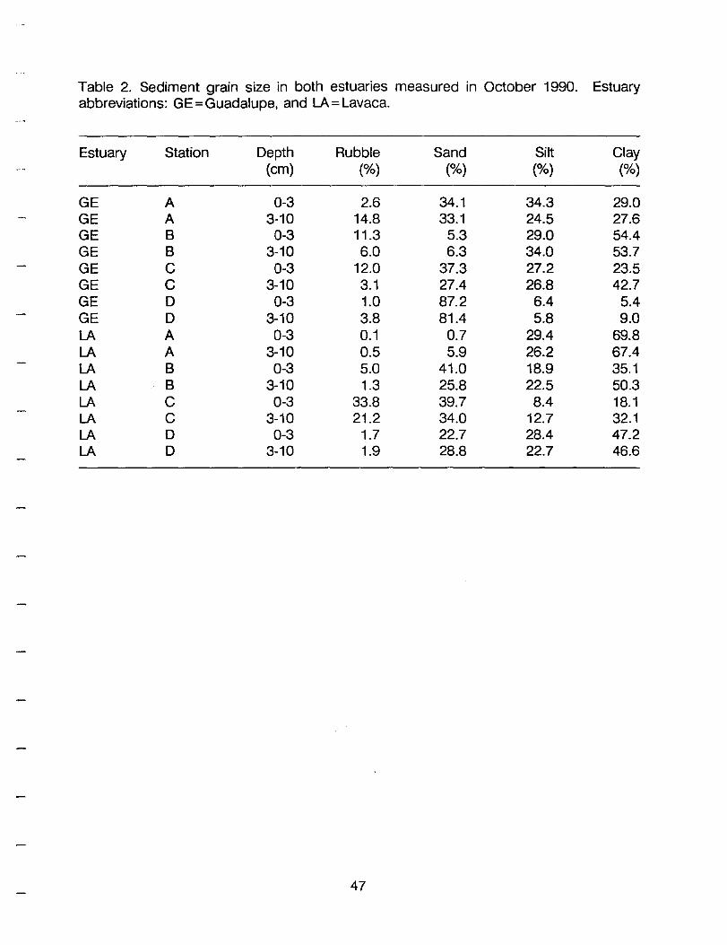
Table 2. Sediment grain size in both estuaries measured in October 1990. Estuary abbreviations: GE=Guadalupe, and LA = Lavaca.

Estuary Station Depth Rubble Sand Silt Clay (cm) (%) (%) (%) (%)

GE A 0-3 2.6 34.1 34.3 29.0 GE A 3-10 14.8 33.1 24.5 27.6 GE B 0-3 11.3 5.3 29.0 54.4 GE B 3-10 6.0 6.3 34.0 53.7 GE C 0-3 12.0 37.3 27.2 23.5 GE C 3-10 3.1 27.4 26.8 42.7 GE D 0-3 1.0 87.2 6.4 5.4 GE D 3-10 3.8 81.4 5.8 9.0 LA A 0-3 0.1 0.7 29.4 69.8 LA A 3-10 0.5 5.9 26.2 67.4 LA B 0-3 5.0 41.0 18.9 35.1 LA B 3-10 1.3 25.8 22.5 50.3 LA C 0-3 33.8 39.7 8.4 18.1 LA C 3-10 21.2 34.0 12.7 32.1 LA D 0-3 1.7 22.7 28.4 47.2 LA D 3-10 1.9 28.8 22.7 46.6

47

Table 3. Sediment carbon and nitrogen inventories in both estuaries measured in October 1990. Estuary abbreviations: GE = Guadalupe, and LA = Lavaca.

Estuary Station Depth Carbon Std Nitrogen Std (cm) (%) (%) (%) (%)

GE A 0-10 3.48 0.09 0.07 0.02 GE A 10-20 3.50 0.28 0.07 0.03 GE A 20-30 3.68 0.32 0.07 0.02 GE A 30-40 3.56 0.28 0.06 0.02 GE A 40-50 3.92 0.16 0.04 0.01 GE A 50-60 4.20 0.37 0.05 0.00 GE A 60-70 4.22 0.10 0.04 0.00 GE A 70-80 3.70 0.21 0.04 0.02 GE A 80-90 3.60 0.08 0.04 0.02 GE A 90-100 3.10 0.32 0.09 0.03 GE B 0-10 3.62 0.01 0.08 GE B 10-20 3.62 0.00 0.07 0.00 GE B 20-30 3.50 0.02 0.11 0.03 GE B 30-40 3.58 0.16 0.07 0.00 GE B 40-50 4.01 0.14 0.07 0.01 GE B 50-60 3.52 0.55 0.06 0.00 GE B 60-70 3.59 0.36 0.07 0.01 GE B 70-80 2.82 0.72 0.06 0.00 GE B 80-90 2.97 0.55 0.06 0.02 GE B 90-100 3.12 0.04 0.06 0.00 GE C 0-10 2.69 0.18 0.03 0.01 GE C 10-20 2.64 0.09 0.04 0.04 GE C 20-30 2.91 0.23 0.05 0.01 GE C 30-40 2.85 0.29 0.05 0.00 GE C 40-50 2.85 0.18 0.05 0.01 GE C 50-60 3.12 0.02 0.06 0.01 GE C 60-70 2.74 0.01 0.04 0.01 GE C 70-80 3.10 0.15 0.04 0.01 GE C 80-90 3.07 0.09 0.03 0.00 GE C 90-100 3.67 0.55 0.02 0.01 GE D 0-10 1.06 0.40 0.02 GE D 10-20 0.73 0.27 0.02 GE D 20-30 0.74 0.13 0.02 0.00 GE D 30-40 0.70 0.30 GE D 40-50 0.82 0.13 0.03 GE D 50-60 0.76 0.15 0.02 GE D 60-70 0.75 0.05 0.02 GE D 70-80 0.67 0.04 GE D 80-90 0.63 GE D 90-100 2.28 1.97 0.01 0.01

48

LA A 0-10 0.98 0.21 0.06 0.01 LA A 10-20 0.96 0.09 0.05 0.01 LA A 20-30 1.05 0.14 0.04 0.01 LA A 30-40 1.36 0.03 0.05 0.03 LA A 40-50 1.07 0.05 LA A 50-60 0.81 0.04 LA A 60-70 0.94 0.12 0.04 LA A 70-80 0.93 0.20 0.03 LA A 80-90 0.80 0.21 0.03 LA A 90-100 1.08 0.04 LA 8 0-10 1.23 0.07 LA 8 10-20 1.17 0.14 0.06 0.02 LA 8 20-30 1.44 0.11 0.07 0.02 LA 8 30-40 1.68 0.03 0.09 0.01 LA 8 40-50 1.54 0.02 0.05 0.03 LA 8 50-60 1.28 0.10 0.04 0.04 LA 8 60-70 1.30 0.04 LA 8 70-80 0.94 0.04 LA 8 80-90 1.30 0.04 LA 8 90-100 1.60 0.07 0.03 0.04 LA. C 0-10 2.47 0.58 0.06 LA C 10-20 2.27 0.73 0.03 0.03 LA C 20-30 1.47 0.30 0.05 LA C 30-40 1.44 0.15 0.04 0.00 LA C 40-50 1.64 0.04 0.04 0.02 LA C 50-60 1.40 0.14 0.03 0.01 LA C 60-70 1.19 0.10 0.05 0.01 LA C 70-80 1.29 0.06 0.05 0.01 LA C 80-90 1.47 0.12 0.07 0.02 LA C 90-100 1.51 0.02 0.06 0.02 LA 0 0-10 1.34 0.12 0.06 0.00 LA 0 10-20 0.74 0.51 0.03 0.03 LA 0 20-30 0.55 0.48 0.04 0.00 LA 0 30-40 0.67 0.05 0.03 0.00 LA 0 40-50 0.54 0.03 0.02 0.00 LA 0 50-60 0.41 0.03 0.01 0.00 LA 0 60-70 0.78 0.60 0.03 0.03 LA 0 70-80 0.69 0.11 0.02 0.00 LA 0 80-90 0.90 0.02 0.03 0.00 LA 0 90-100 0.86 0.04 0.09 0.09

49

Table 4. Guadalupe Estuary macrofauna abundance (n • m·2) and biomass (g • m-2).

Date Station Abundance STD Biomass STD

28JAN87 A 13898 5580 2.024 0.703 03MAR87 A 38953 5604 10.154 9.162 08APR87 A 58805 43356 3.855 2.498 03JUN87 A 57949 27889 9.339 4.262 15JUL87 A 36495 6249 10.656 1.761 18APR88 A 84241 14393 12.985 2.692 07JUL88 A 69198 6806 17.751 1.373 22NOV88 A 23542 4403 11.243 2.398 04APR89 A 101827 7023 8.880 1.004 23JUL89 A 26186 5240 4.781 1.148 05DEC89 A 41317 7618 10.283 1.541 11APR90 A 21651 3226 8.333 2.516 02AUG90 A 44248 2948 5.738 2.177 190CT90 A 16357 3124 3.174 0.594 23JAN91 A 26000 4523 30.276 47.281 22APR91 A 51528 4800 2.032 0.143 28JAN87 B 22124 5587 3.035 1.357 03MAR87 B 19004 6487 4.806 1.432 08APR87 B 20325 433 4.667 1.947 03JUN87 B 21554 8583 7.756 0.870 15JUL87 B 11535 6654 3.528 0.704 18APR88 B 169144 20768 15.364 4.243 07JUL88 B 55491 10673 14.040 2.556 22NOV88 B 34320 6542 23.485 1.591 04APR89 B 63630 5369 6.242 1.606 23JUL89 B 40649 3311 6.068 1.729 05DEC89 B 29877 1931 6.661 4.988 11APR90 B 23731 2129 5.328 0.796 02AUG90 B 25149 2681 4.331 0.490 190CT90 B 14844 1662 1.937 0.959 23JAN91 B 8698 1562 2.470 1.715 22APR91 B 5011 714 1.440 1.613 30JAN87 C 8603 327 1.826 1.917 03MAR87 C 10589 590 2.835 0.772 10APR87 C 11629 1986 5.021 3.047 03JUN87 C 6428 3287 4.185 3.255 15JUL87 C 8698 2979 2.073 1.513 18APR88 C 75259 12918 6.082 0.611 08JUL88 C 18056 2855 1.386 0.513 22NOV88 C 10873 1662 0.688 0.152 04APR89 C 18531 3188 2.260 1.415 23JUL89 C 15031 2878 1.976 0.976

50

05DEC89 C 5578 1428 1.767 0.870 10APR90 C 5389 2141 2.825 2.553 02AUG90 C 8793 5434 2.218 0.943 190CT90 C 23542 3439 2.263 0.442 23JAN91 C 14655 4541 5.826 0.959 22APR91 C 8415 2798 5.727 1.320 30JAN87 D 6428 590 1.386 0.874 03MAR87 D 10495 2215 3.685 0.751 10APR87 D 9264 3523 4.190 1.527 03JUN87 D 7846 433 6.767 4.867 15JULB7 D 3876 912 1.626 1.321 18APR88 D 37155 3070 1.933 0.313 08JULB8 D 11344 2599 0.751 0.350 22NOV88 D 8698 434 1.088 0.148 04APR89 D 25337 9652 8.259 4.467 23JULB9 D 13046 1965 20.909 13.294 05DEC89 D 15884 9952 5.249 1.672 10APR90 D 14182 1985 6.897 1.199 02AUG90 D 10778 2521 2.811 2.228 190CT90 D 15789 6019 1.350 0.433 23JAN91 D 71572 21347 14.373 4.777 22APR91 D 17869 3271 5.284 1.520

51

Table 5. Guadalupe Estuary species list. Average density (n • m-2) over entire study

period.

Taxa A B C D

Cnidaria Anthozoa

Anthozoa (unidentified) 6 a 18 6 Platyhelminthes

Turbellaria Turbellaria (unidentified) 18 6 160 30

Rynchocoela Rhynchocoel (unidentified) 414 467 408 207

Phoronida Phoronis architecta a a 219 71

Mollusca Gastropoda

Gastropoda (unidentified) 780 a a 18 Vitrinellidae

Vitrinellidae (unidentified) a a a 6 Caecidae

Caecum pulchellum a 6 a 6 Caecum johnsoni a a 6 6

Nassariidae Nassarius acutus a a 12 0

Pyramidellidae Odostomia sp_ a a 6 a Turbonilla sp. a a 12 41 Pyramidella crenulata 12 6 6 18 Pyramidella sp. 35 6 a 24

Retusidae Acteocina canaliculata 12 47 24 89

Crepidulidae Crepidula fornicata a a 6 a

Hydrobiidae Littoridina sphinctostoma 15592 5388 1253 266

Pelecypoda Pelecypoda (unidentified) a a 12 41

Nuculanidae Nuculana acuta a a a 12 Nuculana concentrica a a a 6

Mytilidae Brachidontes exustus a 41 a a

Cultellidae Ensis minor 0 6 6 53

52

Leptonidae Mysella p/anu/ata a a a 195

Tellinidae Macoma tenta a a a 6 Tellina sp a 6 a 6 Macoma mitchelli 213 366 124 278

Veneridae Mercenaria campechiensis a a 6 6

Lyonsiidae Lyonsia hyalina f/oridana a a 6 a

Pandoridae Pandora trilineata a a a 6

Sportellidae Afigena texasiana a a 6 77

Mactridae Mu/inia /ateralis 3001 4201 1371 756 Perip/oma cf. orbicu/are a a a 59 Rangia cuneata 30 18 a a

Periplomatidae Perip/oma margaritaceum a a 6 a

Solecurtidae Tage/us p/ebeius a a 24 24

Annelida Polychaeta

Sigalionidae Sigalionidae (unidentified) a a a 6

Palmyridae (= Chrysopetalidae) Pa/eanotus heteroseta a a a 12

Phyllodocidae Eteone heteropoda a 65 6 12 Anaitides erythrophyllus a a 12 a

Pilargiidae Parandalia ocu/aris 53 a 6 30

Hesionidae Gyptis vittata 12 6 53 47 Podarke obscura a a 6 a Hesionidae (unidentified) a a a 6

Syllidae Sphaerosyllis cf. sub/aevis a a a 6 Exogone sp. a a a 12

Nereidae Nereis succinea a a 12 65 Nereidae (unidentified) a a 18 18

Glyceridae G/ycera americana a a a 41 G/ycera capitata a a a 6

53

Goniadidae Glycinde solitaria 6 35 230 260

Onuphidae Diopatra cuprea 0 6 35 59

Arabellidae Drilonereis magna 0 0 6 0

Dorvilleidae Schistomeringos rudolphi 0 0 0 6

Spionidae Polydora ligni 0 0 0 30 Minuspio cirrifera 0 0 0 6 Paraprionospio pinnata 0 18 106 100 Scolelepis texana 0 6 24 41 Polydora websteri 30 0 0 24 Polydora socialis 0 6 59 18 Streblospio benedicti 13105 14286 2127 2541 Polydora caulleryi 0 0 12 1436 Polydora sp. 41 0 0 6 Scolelepis squamata 6 0 47 18 Spionidae (unidentified) 0 6 0 0

Chaetopteridae Spiochaetopterus costarum 0 0 177 1743

Cirratulidae Tharyx setigera 0 0 0 6

Cossuridae Cossura delta 0 0 89 95

Orbiniidae Haploscoloplos foliosus 136 408 331 148 Haploscoloplos fragi/is 0 0 0 12

Capitellidae Capitella capitata 496 148 35 35 Mediomastus californiensis 4384 6257 5897 4668 Notomastus latericeus 0 0 0 6 Heteromastus filiformis 30 0 0 0 Mediomastus ambiseta 4449 2617 1566 2417 Capitellidae (unidentified) 0 0 0 18

Maldanidae Clymenella torquata 0 0 12 95 Asychis sp. 0 0 12 71 Clymenella mucosa 0 0 24 77 Maldanidae (unidentified) 0 0 35 65

Pectinariidae Pectinaria gouldii 0 6 6 6

Ampharetidae Isolda pulchella 0 0 0 6 Melinna maculata 0 6 24 30 Hobsonia florida 804 83 0 0

54

Terebellidae Pista palmata 0 6 118 12 Terebellidae (unidentified) 0 0 0 6

Sabellidae Megalomma bioculatum 0 24 18 24 Sabellidae (unidentified) 0 12 0 0

Serpulidae Eupomatus dianthus 0 0 0 6 Serpulidae (unidentified) 0 0 0 18

Polychaete juv. (unidentified) 0 6 6 0 Oligochaeta

Oligochaetes (unidentified) 236 319 24 0 Crustacea

Copepoda Calanoida

Diaptomidae Pseudodiaptomus coronatus 6 6 24 6

Cyclopoida Cyclopidae

Hemicyclops sp. 0 0 0 12 Cirripedia

Balanus eburneus 18 12 0 0 Malacostraca

Reptantia Callianassidae

Callianassa sp. 0 0 6 6 Pinnotheridae

Pinnixa chacei 0 0 0 6 Pinnotheridae (unidentified) 0 0 0 6

Brachyuran Larvae Megalops 6 6 0 0

Mysidacea Mysidopsis bahia 6 0 6 30 Bowmanie/la sp. 6 0 0 0 Mysidopsis sp. 30 0 0 12 Mysidopsis almyra 18 24 0 0

Cumacea Cyc/aspis varians 30 65 165 26,) Oxyurosty/is sp. 0 0 12 6 Leucon sp. 0 0 47 0 Oxyurosty/is salinoi 0 18 18 18 Oxyurostylis smithi 12 30 201 177

Amphipoda Ampeliscidae

Ampe/isca abdita 30 12 12 30

55

Gammaridae Gammarus mucronatus 6 a 18 a

Oedicerotidae Monoculodes sp. 284 177 160 47 Synchelidium americanum a a a 30

Corophiidae Erichthonias brasiliensis a a a 47 Corophium ascherusicum a 12 a 6 Corophium louisianum a 6 18 a Microprotopus spp. 6 6 6 6

Bateidae Batea catharinensis a a 6 6

Uljeborgiidae Listriella barnardi a 0 6 30

Stenothoidae Parametopella sp. a a a 6

Caprellidae Caprellid 12 a 53 12

Melitidae Elasmopus sp. a a 6 a Melita sp. a a 18 6

Isopoda Anthuridae

Xenanthura brevitelson a 0 a 6 Idoteidae

Edotea montosa a 12 12 a Sphaeromatidae

Cassidinidea lunifrons 0 6 a 0 Echinodermata

Ophiuroidea Ophiuroidea (unidentified) 0 a 6 24

Insecta Pterygota

Diptera Chironomidae

Chironomid larvae 142 35 12 6

56

Table 6. Lavaca-Colorado Estuary hydrographic measurements. Abbreviations: STA = Station, Z = Depth, SAL(R) = Salinity by refractometer, SAL(M) = Salinty by meter, CONO=Conductivity, TEMP=Temperature, OO=dissolved oxygen, and ORP=oxidation redox potential. Missing values show with a period.

Date STA Z SAL(R) SAL(M) CONO TEMP pH DO ORP (m) (ppt) (ppt) (uS/cm) CC) (mg.r') (mV)

18APR88 A 0.00 25 23.7 37.30 24.10 8.50 18APR88 A 1.10 23.7 37.30 18APR88 B 0.00 29 27.3 42.20 23.30 8.80 18APR88 B 2.15 27.2 42.30 23.20 8.00 18APR88 C 0.00 34 31.0 44.80 22.90 18APR88 C 3.10 29.1 47.40 21.60 18APR88 0 0.00 34 31.2 46.90 22.40 8.30 18APR88 0 4.40 30.6 47.70 21.50 19JUL88 A 0.00 28 27.3 42.40 29.90 19JUL88 A 2.00 27.3 42.40 29.90 19JUL88 B 0.00 30 28.6 44.10 30.50 19JUL88 B 2.00 28.6 44.10 30.50 19JUL88 C 0.00 33 31.5 48.20 29.40 6.30 19JUL88 C 2.50 31.5 48.20 29.60 19JUL88 0 0.00 32 32.3 492.0 29.80 19JUL88 0 4.00 32.3 49.20 29.80 22NOV88 A 0.00 32 32.7 49.80 13.80 8.90 22NOV88 A 1.00 32.9 50.00 13.90 8.80 22NOV88 B 0.00 33 34.5 52.20 14.50 8.80 22NOV88 B 1.75 34.6 52.40 14.60 8.60 22 NOV88 C 0.00 35 35.2 53.20 15.40 8.80 22NOV88 C 2.50 35.3 53.30 15.50 8.50 22NOV88 0 0.00 35 34.4 52.10 16.70 8.50 22NOV88 0 4.00 35.1 53.00 16.70 8.30 05APR89 A 1.10 23.0 21.80 05APR89 B 2.10 23.0 20.30 05APR89 C 3.10 23.0 21.40 05APR89 0 4.40 23.0 21.00 22JUL89 A 1.10 22.2 29.50 22JUL89 B 2.10 25.8 29.00 22JUL89 C 3.10 28.2 31.00 22JUL89 0 4.40 36.1 31.00 050EC89 A 0.00 27 10.40 8.00 11.80 050EC89 A 1.50 27 10.20 7.90 11.90 050EC89 B 0.00 28 10.30 7.80 12.20 050EC89 B 2.00 28 10.30 7.80 12.10 050EC89 C 0.00 28 11.30 7.80 11.80

57

05DEC89 C 3.60 28 11.00 7.80 11.20 05DEC89 0 0.00 29 12.40 8.00 10.80 05DEC89 0 4.00 29 12.10 7.80 10.40 10APR90 A 0.00 20 19.4 31.00 19.77 8.23 8.20 10APR90 A 1.50 19.0 31.50 19.77 8.23 8.08 10APR90 B 0.00 20 21.6 33.10 19.96 8.26 8.67 10APR90 B 2.20 20.6 34.60 19.85 8.27 8.15 10APR90 C 0.00 26 26.1 40.50 19.90 8.25 8.15 10APR90 C 3.20 26.0 40.60 19.79 8.25 7.94 10APR90 0 0.00 27 27.6 41.70 20.41 8.34 8.63 10APR90 0 4.60 26.7 42.90 19.95 8.30 7.68 31JUL90 A 0.00 11.9 16.50 31.52 8.66 8.36 1.080 31JUL90 A 1.10 9.4 20.30 31.10 8.49 7.02 1.190 31JUL90 B 0.00 16.5 22.60 30.67 8.43 6.61 0.115 31JUL90 B 1.50 13.5 27.20 30.10 8.31 5.91 0.122 31JUL90 C 0.00 22.3 35.10 31.32 8.29 6.39 0.119 31JUL90 C 2.30 22.0 35.50 30.51 8.27 6.00 0.119 31JUL90 0 0.00 28.4 43.30 29.65 8.25 5.88 0.120 31JUL90 0 3.90 27.9 44.00 29.60 . 8.27 5.73 0.118 230CT90 A 0.00 22 23.5 37.30 19.09 8.17 8.90 0.159 230CT90 A 1.40 26.8 42.00 18.87 8.15 8.07 0.161 230CT90 B 0.00 22 24.7 38.80 18.67 8.18 9.06 0.156 230CT90 B 2.20 27.3 42.90 17.75 8.09 6.64 0.160 230CT90 C 0.00 28 30.9 47.60 19.10 8.24 6.98 0.148 230CT90 C 3.30 31.2 47.90 18.98 8.24 6.79 0.149 230CT90 0 0.00 30 32.3 49.40 18.95 8.29 6.47 0.142 230CT90 0 4.70 32.4 49.50 18.97 8.29 6.35 0.142 25JAN91 A 0.00 6 7.9 14.06 12.43 8.45 12.12 0.145 25JAN91 A 1.10 6 9.5 16.50 10.68 8.43 12.98 0.148 25JAN91 B 0.00 8 8.6 15.20 13.60 8.41 11.71 0.143 25JAN91 B 1.70 8 11.5 19.60 10.72 8.44 11.81 0.147 25JAN91 C 0.00 16 17.2 36.60 10.70 8.19 8.60 0.141 25JAN91 C 2.70 16 22.7 36.60 11.52 8.19 8.60 0.141 25JAN91 0 0.00 20 21.1 33.80 11.96 8.23 9.98 0.147 25JAN91 0 4.20 20 21.9 35.00 11.39 8.16 8.94 0.150 24APR91 A 0.00 3 2.4 5.21 24.98 7.95 8.48 0.143 24APR91 A 1.20 3 2.4 5.23 24.95 7.95 8.26 0.143 24APR91 B 0.00 4 4.3 8.35 24.31 7.92 8.24 0.147 24APR91 B 2.00 4 4.3 8.40 24.30 7.92 8.16 0.148 24APR91 C 0.00 10 10.4 18.10 23.64 7.88 8.03 0.145 24APR91 C 3.10 10 11.8 20.30 23.65 7.84 6.50 0.148 24APR91 0 0.00 20 20.9 33.50 23.79 7.87 7.34 0.152 24APR91 0 4.30 20 23.4 36.90 23.64 7.81 5.74 0.154

58

24JUL91 A 0.00 8 7.4 13.65 29.66 8.40 7.34 0.135 24JUL91 A 1.40 8 7.6 13.72 29.60 8.39 7.10 0.135 24JUL91 B 0.00 12 12.5 20.20 29.98 8.11 6.82 0.149 24JUL91 B 2.10 12 13.1 22.00 29.53 8.12 6.38 0.136 24JUL91 C 0.00 21 20.6 33.10 29.64 7.68 6.12 0.211 24JUL91 C 3.10 21 23.9 37.70 30.02 7.50 2.89 0.215 24JUL91 D 0.00 32 31.4 48.30 29.70 7.85 5.19 0.170 24JUL91 D 4.50 32 32.6 49.50 29.73 7.67 3.18 0.175

"

59

Table 7 . Lavaca-Colorado Estuary macrofauna abundance (n • m-2) and biomass (g • . 2) m.

Date Station Abundance STD Biomass STD

28NOV84 A 8149 2521 23JAN85 A 8451 4803 06MAR85 A 7621 3524 03APR85 A 5961 1925 08MAY85 A 7319 1699 05JUN85 A 7847 3073 17JUL85 A 7092 2483 14AUG85 A 5357 915 220CT85 A 3546 692 04DEC85 A 2113 653 05FEB86 A 6036 1898 09APR86 A 14109 2911 04JUN86 A 7319 2267 06AUG86 A 5357 795 18APR88 A 29499 1771 7.381 2.875 19JUL88 A 7941 1725 0.824 0.633 22NOV88 A 9170 1181 2.687 1.577 05APR89 A 26757 6344 10.678 7.117 22JUL89 A 8035 2412 3.790 1.532 05DEC89 A 7658 2269 0.760 0.455 10APR90 A 14560 867 7.956 2.892 31JUL90 A 4349 1845 2.808 4.143 230CT90 A 2269 750 0.208 0.046 25JAN91 A 1702 851 0.039 0.026 24APR91 A 1891 912 1.082 1.787 18APR88 B 18531 2412 2.605 0.494 19JUL88 B 11249 3124 1.886 1.578 22NOV88 B 8508 1860 0.667 0.450 05APR89 B 11629 2948 5.549 2.101 22JUL89 B 8508 2947 1.812 1.083 05DEC89 B 9455 1456 3.604 2.949 10APR90 B 12575 3592 3.418 1.567 31JUL90 B 4444 590 1.330 0.963 230CT90 B 10400 3324 2.004 1.326 25JAN91 B 11251 1279 2.896 1.116 24APR91 B 3593 655 0.797 0.332 18APR88 C 32334 12286 13.456 12.015 19JUL88 C 17961 7553 5.989 3.402 22NOV88 C 14369 2147 4.429 1.452 05APR89 C 8226 4292 8.055 9.434 22JUL89 C 4821 2423 1.089 1.340

60

05DEC89 C 17586 7057 8.484 3.390 10APR90 C 22975 4687 9.729 5.110 31JUL90 C 22313 8069 7.154 1.831 230CT90 C 42073 4932 51.454 34.782 25JAN91 C 25149 5746 16.861 7.671 24APR91 C 22218 4766 13.160 4.084 18APR88 D 101340 47872 12.249 4.113 19JUL88 D 25808 3196 10.579 5.802 22NOV88 D 41027 7851 3.817 1.118 05APR89 D 29782 2947 28.041 25.082 22JUL89 D 22972 3001 43.350 23.086 05DEC89 D 17397 4248 35.999 17.594 10APR90 D 25244 4643 26.730 13.264 31JUL90 D 12669 3934 6.370 5.801 230CT90 D 8604 1~89 9.814 3.021 25JAN91 D 15317 1300 5.895 2.275 24APR91 D 37440 10506 28.549 18.105

61

Table 8. Lavaca-Colorado Estuary species list. Average density (n • m-2) over entire

study period.

Taxa A B C 0

Cnidaria Anthozoa

Anthozoa (unidentified) 0 17 17 95 Platyhelminthes

Turbellaria Turbellaria (unidentified) 17 9 60 60

Rynchocoela Rhynchocoel (unidentified) 34 103 567 902

Phoronida Phoronis architecta 0 69 17 52

Mollusca Gastropoda

Gastropoda (unidentified) 9 9 9 0 Caecidae

Caecum johnsoni 0 0 17 34 Columbellidae

Mitrella lunata 0 0 9 0 Nassariidae

Nassarius acutus 34 43 34 34 Nassarius vibex 0 0 0 17

Pyramidellidae Odostomia sp. 26 17 0 0 Turbonil/a sp. 0 26 103 9 Pyramidella crenulata 26 77 17 0 Pyramidella sp. 26 34 9 0

Retusidae Acteocina canaliculata 146 120 17 17

Crepidulidae Crepidula fornicata 0 0 0 26

Hydrobiidae Uttoridina sphinctostoma 17 0 0 0

Scaphopoda Dentaliidae

Dentalium texasianum 0 0 0 17 Pelecypoda

Pelecypoda (unidentified) 43 26 43 576 Nuculanidae

Nuculana acuta 0 0 9 60 Nucu/ana concentrica 26 52 43 43

Arcidae Anadara ova/is 0 0 0 9

62

Cultellidae Ensis minor 120 0 0 0

Leptonidae Mysel/a planulata 34 26 0 17

Tellinidae Macoma tenta 0 0 0 17 Teflina sp 69 52 0 9 Tellina texana 0 0 0 9 Macoma mitchelli 60 52 9 0

Semelidae Abra aequalis 0 0 0 95

Veneridae Mercenaria campechiensis 0 0 0 9

Corbulidae Corbula contracta 0 0 0 1057

Pandoridae Pandora trilineata 0 17 0 0

Sportellidae A1igena texasiana 0 0 17 0

Mactridae Mulinia /ateralis 859 455 34 26 Perip/oma cf. orbiculare 0 0 129 1693

Periplomatidae Periploma margaritaceum 0 0 34 0

Solecurtidae Tagelus p/ebeius 69 0 0 0

Hiatellidae J

Hiatel/a arctica 0 0 0 138 Annelida

Polychaeta Polychaete juv. (unidentified) 0 17 9 69

Polynoidae Eunoe cf. nodulosa 0 0 0 34 Polynoidae (unidentified) 0 0 0 9

Sigalionidae Sigalionidae (unidentified) 0 0 52 69

Palmyridae (= Chrysopetalidae) Paleanotus heteroseta 0 0 120 421

Phyllodocidae Eteone heteropoda 9 0 0 9 Anaitides erythrophyl/us 9 0 0 0 Phyllodocidae (unidentified) 9 0 0 0

Pilargiidae Sigambra tentaculata 0 0 0 86 Ancistrosyllis groenlandica 0 0 9 17 Ancistrosyllis papillosa 0 0 9 17 Parandalia ocularis 69 0 17 0

63

Ancistrosyllis cf. fa/cata a a a 9 Sigambra cf. wassi a a a 9 Pilargiidae (unidentified) a a 9 17

Hesionidae Gyptis vittata 17 26 524 232 Podarke obscura a a 9 17

Syllidae Sphaerosyllis ct. sublaevis a a a 9 Sphaerosyllis erinaceus a a 9 9 Brania clavata a a 455 9 Sphaerosyllis sp. A 26 17 26 163 Syllidae (unidentified) a a 60 9

Nereidae Ceratonereis irritabilis a a 9 a Laeonereis culveri 9 9 a a Nereidae (unidentified) 34 a 17 86

Nephtyidae Aglaophamus verrilli a a a 9

Glyceridae G/ycera americana a 9 43 26 Glycera capitata a a a 9 Glyceridae (unidentified) 43 9 a a

Goniadidae Glycinde solitaria 370 163 275 138

Onuphidae Diopatra cuprea 34 34 43 52

Arabellidae Drilonereis magna a 9 1246 129

Dorvi/leidae Schistomeringos rudolphi a a 9 26 Schistomeringos sp. A a a 26 a

Spionidae Polydora Iigni 52 a 9 a Minuspio cirrifera a a 395 1323 Paraprionospio pinnata 77 292 206 146 Apoprionospio pygmaea a a 17 a Scolelepis texana a 9 a a Polydora socialis a a 146 9 Streblospio benedicti 1229 2234 309 26 Polydora caulleryi a a 2432 1427 Polydora sp. a a a 26 Scole/epis squamata 17 a a a Spionidae (unidentified) a a 52 541

Magelonidae Magelona pettibaneae a a 26 a Magelana phyllisae a a 9 9

Chaetopteridae

64

Spiochaetopterus costarum 43 34 206 17 Cirratulidae

Cirriformia filigera 0 0 9 0 Tharyx setigera 0 0 1435 17

Cossuridae Cossura delta 241 679 438 567

Orbiniidae Haploscoloplos foliosus 77 112 34 103 Naineris laevigata 0 0 17 352

Paraonidae Paraonidae Grp. A 0 0 275 34 Paraonidae Grp. B 0 0 963 524

Opheliidae Armandia maculata 0 0 0 69

Capitellidae Capitella capitata 26 9 0 0 Mediomastus californiensis 3334 2870 3730 4142 Notomastus latericeus 0 0 9 34 Notomastus cf. latericeus 0 0 26 52 Heteromastus filiformis 112 34 0 0 Mediomastus ambiseta 816 1461 3369 1899 Capitellidae (unidentified) 0 0 17 9

Maldanidae Branchioasychis americana 9 17 223 34 Clymenella torquata 17 0 103 26 Asychis sp. 9 0 258 0 Clymenella mucosa 52 69 318 17

- Maldanidae (unidentified) 0 69 163 77 Oweniidae

Owenia fusiformis 0 0 17 0 Flabelligeridae

Brada ct. villosa capensis 0 0 0 9 Pectinariidae

Pectin aria gouldii 0 0 0 9 Ampharetidae

Melinna maculata 17 34 77 9 Terebellidae

Amaenana trilobata 0 0 52 34 Pista palmata 0 0 17 0 Terebellidae (unidentified) 0 0 9 43

Sabellidae Sabella microphthalma 0 0 17 0 Megalomma bioculatum 0 9 17 0

. Sabellidae (unidentified) 0 0 9 0 Oligochaeta

Oligochaetes (unidentified) 0 0 86 756

65

Sipuncula Phascolion strombi a a 9 138 Sipuncula (unidentified) a a a 9

Crustacea Ostracoda

Myodocopa Sarsiella texana 17 a 17 a Sarsiella spinosa a a 9 9

Copepoda Calanoida

Diaptomidae Pseudodiaptomus coronatus 9 34 26 43

Cyclopoida Cyclopidae

Hemicyclops sp. 9 a a a Uchomolgidae

Cyclopoid copepod (commensal) 95 26 a a Malacostraca

Natantia Ogyrididae

Ogyrides Iimicola a 9 9 a Reptantia

Paguridae Pagurus annuli pes a a a 26 Pagurid juv. a a 17 a

Portunidae Callinectes similis a a 9 a

Xanthidae Xanthidae (unidentified) a a 9 a

Pinnotheridae Pinnixa sp. a a a 43 Pinnixa cristata a a 17 a Pinnixa chacei a a 17 120 Pinnixa retinens a a. 17 a Pinnotheridae (unidentified) a a a 9

Brachyuran Larvae Megalops a a a 9

Mysidacea Mysidopsis bigelowi a a 60 a Mysidopsis bahia 17 9 26 17 Mysidopsis sp. a 26 9 9

Cumacea Cyclaspis varians 95 103 a a Oxyurostylis sp. a 9 26 9 Leucon sp. 77 120 9 a Oxyurostylis salinoi a a 138 a Oxyurosty/is smithi 86 17 43 9

66

Eudorella sp. a 43 17 a Amphipoda

Amphipoda (unidentified) a a 9 17 Ampeliscidae

Ampelisca sp. B a a 9 43 Ampelisca abdita 1461 138 52 9 Ampelisca verrilli a a 17 a

Gammaridae Gammarus mucronatus 9 a a a

Oedicerotidae Monoculodes sp. 26 17 26 a

Corophiidae Erichthonias brasiliensis a a a 34 Ph otis sp. a a 17 a Microprotopus spp. 26 17 a a

Liljeborgiidae Listriella barnardi 9 9 52 60 Listriella clymenellae a a 17 a

Caprellidae Caprellid 9 a 17 9

Amphilochidae Amphilochus sp. a a 9 a

Isopoda Idoteidae

Edotea montosa 34 a a a Tanaidacea

Apseudidae Apseudes sp. A a a 9 9840

Echinodermata Ophiuroidea

Ophiuroidea (unidentified) a a 249 576 Chordata

Hemichordata Schizocardium sp. a 9 284 610

67

EFFECTS OF THE LAGUNA MADRE, TEXAS BROWN TIDE ON BENTHOS

The Brown Tide Event

In January 1990, a bloom of an undescribed species of a chysophyte began in the

upper reaches of Baffin Bay, Texas bordering the King Ranch. The chrysophyte is a

small (5 JLm in diameter) single cell diatom, with a crescent-shaped chloroplast. Bloom

conditions did not exist until later in the spring. In fact, the brown tide was not noticed

until it reached the adjacent Laguna Madre (Figure 1). The brown tide went unnoticed

for 5 months, because it occurred in an unpopulated area. Sport or commercial

fisherman did not report the event either. In the Laguna Madre it could not go unnoticed. The chlorophyll content in the water increased by almost two orders of magnitude, and

the visibility over the seagrass beds dropped from 10 feet to less than 1 inch. You could

not see you hand when it was placed just below the surface of the water. Once the

brown tide bloom reached the Laguna Madre, it quickly spread to adjacent estuaries. By

late summer 1990, the prevailing south-westerly winds had spread the tide north to (but

not in) San Antonio Bay. The wind-reversing northerlies of fall 1990 and winter 1991

reversed the brown tide movement. The southern (or lower) Laguna Madre was

completely covered during this period. Over the entire year the brown tide covered an area of about 150 linear miles. A wet spring and summer in 1991 has led to a decline in

the bloom conditions, but the chrysophyte is still present.

It is impossible to know, in hindsight, exactly what caused the brown tide bloom.

However, since several research projects were in progress at the time, more is probably

known about the causes and effects of this brown tide than any other. Several events

were coincident at the outset of the brown tide suggesting that there were multiple

causes, and that they must occur at the same time, since these events occurred by

themselves regularly in the past without causing brown tides. The 2-year period

preceding the brown tide was very dry. Salinities rose from 30 ppt in 1986 to 45 ppt in

1989 during the drought. During the spring of 1990, the drought was broken by a spring

flood event that elevated nutrient levels in Baffin Bay and Laguna Madre. There was also a freeze in December 1989 just prior to the first signs of the brown tide. The freeze

occurred during a period of low tides. The combination of cold and shallow water led to

an enormous fish kill. This resulted in an enormous amount of nitrogen, which had been

locked up in fish biomass, being released into the water. It is probable that the combination of the freeze coming after a drought was the primary cause of the brown

tide. Nutrients were dumped into a system that had low diversity, low stability, and was

68

•

nutrient depleted. These are ideal conditions for a bloom event. Other conditions were

also present and could have had a role in causing the bloom. Maintenance dredging was

being performed in the Intracoastal Waterway (lCW), and the King Ranch had put a large

tract close to Baffin Bay in agriculture. Finally, Baffin Bay and Laguna Madre are

characterized by little circulation, and a microtidal range. The lack of adequate circulation

also contributed to low flushing of the bloom organism.

The immediate concern of the brown tide was that the concomitant water transparency

and light reductions could lead to loss of seagrass bed habitats. The degradation of the

habitats would be an environmental disaster. The Laguna Madre and Baffin Bay have

great value. This region of the Texas coast yielded 53% of the total commercial finfish

harvest during the last 20 years. It is an overwintering ground for the endangered

redhead ducks. It is one of the last relatively pristine areas, the human population density

is low, and it is bordered by the King Ranch on one side and the Padre Island National Seashore on the other side. The principal human activities in the area are tourism, oil and gas production, and transportation (via the ICW). The local tourism and fishing industry

was devastated by the brown tide during the summer of 1990, but has recovered

significantly in the summer of 1991. Although, the potential for negative effects on

seagrass exists, it probably has not occurred. The seagrasses had enough carbon

stored in roots to survive and grow during the brown tide (at least down to a depth of 1 -

1.3 m). Fortunately, the beds were mapped in 1988 by the U.S. Fish and Wildlife Service

and they plan a post-brown tide survey. Until the beds are mapped again, the extent of

effects on seagrass won't be known.

The Effect of Brown Tide on Benthos

The main effect of brown tide on benthos in other areas of the U.S. was the decline

of bivalve mollusk densities due to clogging of feeding appendages by the small

chrysophyte. This led to a severe economic loss in shellfish fisheries of the northeast.

In Texas, there is a climatic gradient from northeast to southwest of decreasing rainfall

and concomitantly decreasing freshwater inflow to estuaries. Due to a lack of sufficient

inflow, only the northeastern estuaries of Texas support a commercial oyster industry. Therefore, the economic effects of brown tide in south Texas would not be direct effects

on benthos, but indirect effects could alter food webs and have dramatic consequences.

A variety of benthic studies have been performed to examine productivity of (both

autotrophic and heterotrophic) microbial producers, and abundance and community

structure of macro benthic organisms. These studies were performed in Baffin Bay and

69

the upper Laguna Madre. Benthic nutrient regeneration, oxygen consumption, and

bacterial biomass and productivity were studied bimonthly for one year before the brown tide event. Biomass, productivity and responses to light by microphytobenthos were

studied before and after the brown tide. Macrofauna were sampled bimonthly until

January 1990 and quarterly thereafter.

Baffin Bay is deeper and more turbid than the Laguna Madre, so one may suppose

that benthic primary production by microphytobenthos is low. Prior to the brown tide, the

shade-adapted microphytobenthos produced up to 3 g C·m·2 ·d·1 in Baffin Bay sediments

(Figure 2). The amount fluctuates daily, decreasing with wind-induced resuspension of

sediments, which blocks light reaching the bottom. After the brown tide, no benthic

photosynthesis occurred because of a lack of light reaching the bottom (Figure 3). This

represents a great loss of autotrophic production, and consequently high quality food, to

the benthic food web.

Sediment bacterial production is correlated with bacterial cell abundance (Table 1). Sediment oxygen consumption and inorganic nitrogen regeneration are correlated with

bacterial production. Baffin Bay sediments are sources of regenerated nitrogen, and

Laguna Madre sediments are sinks for nitrogen. The uptake of nitrogen by Laguna

Madre sediments is probably due to absorption by seagrass roots.

There are indications that a disturbance of some sort was already occurring in the

sediments of Baffin Bay and Laguna Madre prior to the brown tide. In early 1989, the

macrofauna community was very abundant and diverse. However, from August 1989 to

January 1990, abundance was increasing while diversity was decreasing (Figures 4-5). The community in Baffin Bay was dominated by a single species, the polychaete worm

Streb/ospio benedicti (Table 2). This pattern is typical of a disturbed benthic community.

During the onset of the brown tide, abundances and diversity decreased to near zero.

As found in the northeast, bivalve mollusks disappeared within weeks after the brown tide onset. Baffin Bay is now completely dominated by Streb/ospio, while Laguna Madre is

dominated by polychaetes and gastropods. Streb/opsio is a suspension feeder and a

deposit feeder. There has been a complete alteration of the benthic food web. The loss

of the bivalves, particularly Mulinia lateralis, is of great concern, since it is reported to be

the dominant food source of black drum. The hypersaline Baffin Bay-Laguna Madre ecosystem is a very fragile environment.

This is indicated by the lack of stability in the ecosystem. When the equilibrium was put

out of balance by the loss of diversity, the benthic system rapidly deteriorated and

crashed. This crash could be either a pre-condition, causal mechanism, or a contributing

factor for the onset of the brown tide. The ecosystem was apparently already disturbed and did not have the stability to withstand further disturbance. An alternative hypothesis

70

is that what ever caused the disturbance that led to the benthic response before the

brown tide also caused the brown tide. If this is true then benthos could play the role of

"canary" to future blooms.

71

Table 1. Descriptive statistics of microbial and sediment variables by station over the entire study period. Variables are fol1wed by abbrieviations in parentheses. Statistics include mean ± standard error and number of observations in parentheses.

STATION

VARIABLE UNITS VEGETATED BARE-PATCH MUD

Bacterial abundance (BA) 109 ce11s ocm-3 5.41 ± 3.08 (36) 3.25 ± 2.76 (36) 5.72 ± 1.43 (36) Bacterial production (BP) fJ.g Cocm- 3oh-1 1.78 ± 2.13 (36) 0.43 ± 0.51 (36) 1.92 ± 2.09 (36) Specific growth rate (SGR) d- 1 0.25 ± 0.23 (36) 0.12 ± 0.11 (36) 0.28 ± 0.31 (36) , Oxygen metabolism (OM) mmol om- 2oh-1 3.96 ± 2.12 (48) 1.42 ± 0.71 (48) 0.87 ± 0.46 (48) Dissolved organic carbon (DOC) fJ.g Cocm- 3 30.7 ± 11.0 (36) 24.6 ± 7.86 (36) 14.6 ± 3.14 (36) Total organic carbon (TOC) mg Cocm-3 13.6 ± 4.27 (11) 11.1 ± 2.52 (11) 5.99 ± 1.73 (11) Organic carbon content (C) Yo 1.96 ± 0.76 (11) 1.27 ± 0.90 (11) 1. 82 ± 0.11 (11) Total organic nitrogen (TON) mg Nocm- 3 0.96 ± 0.26 (11) 0.78 ± 0.26. (11) 0.64 ± 0.10 (11) Organic nitrogen content (N) Yo 0.14 ± 0.08 (11) 0.09 ± 0.09 (11) 0.20 ± 0.04 (11)

--J f\) Molar C to N ratio (CN) 16.6 ± 2.5 (11) 17.5 ± 4.6 (11) 10.8 ± 1.6 (11)

Ammonium concentration (NH4) fJ.M 55.3 ± 34.4 (36) 72.9 ± 60.6 (36) 138 ± 88.6 (36) Nitrite concentration (N02) fJ.M 3.47 ± 2.84 (36) 2.35 ± 3.73 (36) 2.38 ± 3.56 (36) Nitrate concentration (N03) fJ.M 4.11 ± 6.60 (36) 1.89 ± 3.26 (36) 3.77 ± 7.09 (36) Chlorophyll concentration' (CHL) mg f m- 2 20.8± 7.97 (36) 27.6 ± 8.38 (36) 11.1 ± 6.70 (36) Phaeopigment concentration' (PHA) mg om- 2 111 ± 21.7 (35) 64.9 ± 17.3 (36) 59.1 ± 10.4 (36) Water content (W) Yo 45.7 ± 13.4 (11) 36.6 ± 14.3 (11) 72.7 ± 6.80 (11) Percent sandb (SA) Yo 77.07 (1) 81.55 (1) 30.67 (1) Percent siltb (SI) Yo 0.92 (1) 3.64 (1) 15.41 (1) Percent clayb (CL) Yo 5.71 (1) 3.99 (1) 48.36 (1)

, integrated to 1 cm depth. b Results of single samples of 0-3cm strata sediment collected during the March 1989 sampling.

Table 2. Macrofauna community composition over two years. Brown tide started in

January 1990 in Baffin Bay, and reached Laguna Madre in June 1990. Table finds

average percent abundance from 6 replicates.

1989 1990

Taxa Mar May Jul Nov Jan Apr Jul Oct

BAFFIN BAY

Mollusca 29 28 0 1 1 12 2 0

Polychaeta 63 66 t99 98 99 88 97 100

Crustacea 8 4 0 1 0 0 1 0

Other 0 2 1 0 0 0 0 0

LAGUNA MADRE

Mollusca 23 14 17 14 10 t80

Polychaeta 70 55 70 76 84 18

Crustacea 6 30 10 9 3 2

Other 1 1 3 1 3 0

tstart Streb/ospio benedicti dominance

tall Gastropoda

73

CORPUS CHRISTI

BAY

t :n

Study Area I

GULF

OF

MEXICO

Figure 1. Study area. Stations sampled are marked with stars. The two stations in

Laguna Madre were paired seagrass bed (Halodule wrightil) and bare patch stations.

74

o 9:00 '" 13:00 [] 16:00 25 . ----~------------ ---~---------,

L

.c

~ 20 E

I ...J 15 :r () (]l

E () 10 (]l

E

c o

:.:; o :J

U o L.

5

(A) o 0 o

o o o

b.

o co 0 o

o o o o

D- O~----------~----------~----------.-----------~ o 500 1000 1500 2000

Irradiance Cumol·m- 2 ·sec-,:-1)

3500~--------------------------------------------~

~

'I .3000 >­o

<:? 2500 N I

~ 2000 () (]l

S 1500 c o

=t; 1000 :J

U o L.

D- 500

(8)

1990

Figure 2. Microphytobenthos primary production. (A) Production as a function of light

irradiance during the day. (8) Modeled daily production based on bottom light

measurements and photosynthetic parameters calculated from A.

75

m CS

0.20 ~ ---I 0-

...c 2 ---~

R 0.82 ---~ - ---~ I 0.15 ---I --..-----.. a ~

I ...c. UJ

U N. 0.10 --I --(]l E -- 0 --E ------0 0.05 --U --E -----(]l ::t. C E '-../ ~ '--' 0.00

0 200 400 600 800

(Jl-mol -2 -1

lrradiance m s )

Figure 3. Effect of brown tide an photosynthetic parameters of microphytobenthos.

o=May 1990 (before brown tide) and D=July 1990 (during brown tide).

76

"~-----------'------

Q) ()

c o " C ::J .0 «

8E4

6E4

4E4

2E4

0 F A 1989

Effect of Brown Tide on Macrobenthos

•

J A 0 0 F 1990

.-.Baffin Bay

0-0 laguna Madr

~ "" 0

A J A 0 0

Figure 4. Effect of brown tide on macrobenthos abundance in Baffin Bay and Laguna

Madre. Brown tide appeared at these station in June 1990.

77

Effect of Brown Tide on Macrobenthos

24

L 0 __

.-.Baffin Bay Ql 20 I -0

..Q \ E I 0- -0 Laguna Madr :J I \ z 16 \ >. I \ ....... Vl I \ L Ql 12 I 0--0 >

0 0 '\. '\. .- 0 __ z 8

Vl '--- ~

---I 4 .-e --~ -- -0

0 .-. • F A J A 0 0 F A J A 0 0 1989 1990

Figure 5. Effect of brown tide on macrobenthos diversity in Baffin Bay and Laguna

Madre. Hill's diversity number is a measure of the number of dominant species.

78