17
The use of CFD for heliostat wind load analysis A.V. Hariram, T.M Harms & P. Gauché Solar Thermal Energy Research Group (STERG)

The use of CFD for heliostat wind load
analysis
A.V. Hariram, T.M Harms & P. Gauché
Solar Thermal Energy Research Group (STERG)

Introduction: Why CFD?
• Heliostat field can make up to 40% of central receiver
plant’s cost
• Cost reduction in development of heliostats could have
major cost saving implications
• Can be achieved by designing heliostats based on wind loads
and to not overdesign them
• Wind loads traditionally acquired through wind tunnel
testing
• Wind tunnel testing can be time consuming and expensive,
with CFD providing an alternative method to determine
wind loads
2

Past CFD work
• To my knowledge, only 2 previous numerical studies on full
3-D heliostats
• Sment and Ho investigated velocity profiles above a heliostat
predicted by CFD with comparison to full scale field
measurements
• Wu and Wang looked at load and moment coefficients with
comparison to experimental results, concluding that CFD
would be a useful tool in this area
3
Simulations from Sment and Ho

CFD Methods Chosen
• RANS modelling methods chosen for this study due to it being
essentially a first study; simple approach desired
• Three turbulence models of interest were RNG-k-ε, Realisable-k-ε and SST-k-𝜔
• Complete analysis including mesh independency and strong
possibility of transient analysis with all three models not viable
in time available
• Single model to be chosen to move forward with for complete
analysis
• Selection of model based on simulation of flat plate
perpendicular to the flow in two orientations (next slide)
• Geometry very similar to a heliostat with reported results for
drag and velocity fluctuations in the wake makes for an ideal
test case
4

Flat Plate Orientations
5
Flow direction
Two orientations: Gap at lower edge of plate (left) and
ground mounted (right)
Gap

Flat Plate Simulation
• These simulations used same mesh and settings across all
models to isolate effect of just turbulence model
• Mesh independency also achieved with each model to
ensure results only affect by modelling techniques
• First result investigated was drag coefficient:
• Results show that the Realisable-k-ε model predicts the drag
the closest whilst the other two models show similar
accuracy to each other
6
Realisable-k-ε RNG-k-ε SST-k-ω
Simulation 1.13 1.11 1.17
Experimental 1.14 1.14 1.14
Error -0.87 % -2.63 % 2.63 %
Flat Plate Simulation
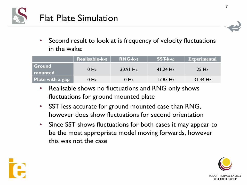
• Second result to look at is frequency of velocity fluctuations
in the wake:
• Realisable shows no fluctuations and RNG only shows
fluctuations for ground mounted plate
• SST less accurate for ground mounted case than RNG,
however does show fluctuations for second orientation
• Since SST shows fluctuations for both cases it may appear to
be the most appropriate model moving forwards, however
this was not the case
7
Realisable-k-ε RNG-k-ε SST-k-ω Experimental
Ground
mounted0 Hz 30.91 Hz 41.24 Hz 25 Hz
Plate with a gap 0 Hz 0 Hz 17.85 Hz 31.44 Hz

Model Selection
• Realisable model actually chosen moving forward for a few
reasons
• One major factor is dataset from Peterka and associates,
used to validate CFD results, does not contain transient
data meaning transient data from CFD cannot be validated
• Transient simulations also require undesirable amounts of
time to obtain results that cannot be full validated
• Since Realisable model produced most accurate drag
coefficient and considering only time-averaged load
coefficients are available for validation, Realisable was
chosen to move forward
8

Heliostat Simulation
• Once Realisable model chosen to move forward, simulations
for heliostat based on Peterka et al. were conducted
9
Geometry used in CFD (left) and experimental geometry from
Peterka et al. (right)

Heliostat Simulation
• Simulations conducted to reproduce similar upstream
turbulence and velocity profiles for a heliostat on two
orientations.
10
Oriented perpendicular to the flow (left) and at 45° to both the
ground and flow (right)
Flow direction

Heliostat Simulation
• First look at the upstream velocity and turbulence profiles
produced compared to experimental profiles:
• Turbulence matches well whereas velocity can be seen to
show some inaccuracy near the ground
11
0
0.2
0.4
0.6
0.8
1
0 2 4 6 8 10
No
rmalise
d h
eig
ht
Turbulence intensity (%)
Turbulence intensity profile
CFD
Experimental
0
0.2
0.4
0.6
0.8
1
0 0.2 0.4 0.6 0.8 1 1.2N
orm
alise
d h
eig
ht
Normalised velocity
Normalised velocity profile
CFD
Experimental

Heliostat Simulation
• Results of concern are various load and moment coefficients
such as 𝐶𝐹𝑋 (drag) and 𝐶𝑚𝑦(overturning moment):
12
Various load and moment coefficients from Peterka et al.

Heliostat simulation
• For perpendicular orientation, only the drag and overturning
moment about base are considered as other reported
coefficients are small and thus can be sensitive to
measurement errors making the CFD results appear
inaccurate
• At this orientation, it can be seen that values are slightly
over predicted, yet are still quite accurate
• Overturning difference likely due to difference in velocity
profile
13
𝑪𝑭𝒙 (Drag) 𝑪𝒎𝒚𝒃𝒂𝒔𝒆(Overturning moment about base)
CFD -1.265 -0.647
Experimental -1.171 -0.635
Error 8.02 % 1.89 %

Heliostat simulation
• For the angled orientation, again only some coefficients are
considered:
• Drag prediction accuracy decreased whilst lift prediction is
quite accurate
• Moment prediction inaccurate with likely cause again being
the differing velocity profile
• Other cause of inaccuracies could be the geometric
simplifications affecting the flow field
• Could be RANS cannot accurately predict complex flow
features associated with bluff body flows
14
𝑪𝑭𝒙(Drag) 𝑪𝑭𝒛(Lift) 𝑪𝒎𝒚𝒃𝒂𝒔𝒆(Overturning moment about base)
CFD -0.724 -0.690 -0.387
Experimental -0.556 -0.672 -0.208
Error -23.20 % -2.6 % -46.25 %

Conclusions
• CFD can potentially be used to estimate basic loading
coefficients
• RANS modelling techniques not appropriate to capture all
relevant information required for a complete heliostat
design
• Even with inaccuracies predicted from CFD, it can still be
useful in comparing heliostat designs early in the process
15

Current and Future Work
• Involved in post-processing of PIV data acquired with Danica
Bezuidenhout for a heliostat with a simpler geometry than
Peterka et al.
• Simulations conducted with partial lower atmospheric
boundary lower turbulence and velocity profiles
• If computing power allows, LES or hybrid RANS-LES models
would be the most appropriate to model flow over a
heliostat
16

Thank you!
17
Acknowledgements:
Contact details:Author A.
Thermal Energy Research Group
(STERG)
University of Stellenbosch
Stellenbosch
South Africa
+27 (0)21 808 4016
Visit us:
concentrating.sun.ac.za
blogs.sun.ac.za/STERG
Acknowledgements: Contact details:
A.V. Hariram
Solar Thermal Energy Research
Group (STERG)
University of Stellenbosch
South Africa
STERG
University of Stellenbosch
ESKOM


