The Use of Hourly Model-Generated Soundings to Forecast...

DECEMBER 1998 1165F O R E C A S T I N G T E C H N I Q U E S

q 1998 American Meteorological Society

FORECASTING TECHNIQUES

The Use of Hourly Model-Generated Soundings to Forecast Mesoscale Phenomena.Part I: Initial Assessment in Forecasting Warm-Season Phenomena

ROBERT E. HART AND GREGORY S. FORBES

Department of Meteorology, The Pennsylvania State University, University Park, Pennsylvania

RICHARD H. GRUMM

National Weather Service, State College, Pennsylvania

16 December 1997 and 14 July 1998

ABSTRACT

Since late 1995, NCEP has made available to forecasters hourly model guidance at selected sites in the formof vertical profiles of various forecast fields. These profiles provide forecasters with increased temporal resolutionand greater vertical resolution than had been previously available. The hourly forecast profiles are provided forall of NCEP’s short-range models: the Nested Grid Model, Eta Model, and Mesoscale Eta Model. The high-resolution forecasts aid in the timing of frontal passages, low-level jets, and convective initiation. In addition,through time–height cross sections of Richardson numbers, forecasters can alert pilots to the potential for clearair turbulence several hours to a day in advance. Further, the profiles are useful in prediction of cloudiness andthe dissipation of low-level stratus and fog. Time–height cross sections of wind velocity have proven extraor-dinarily useful in visualizing and forecasting inversion heights, frontal passage timing, boundary layer depth,and available environmental and storm-relative helicity during convective events.

The hourly model forecasts were found to be exceptionally helpful when combined with hourly surfaceobservations to produce enhanced real-time analyses of convective parameters for use in very short term fore-casting. High-resolution analyses of lifted index, CAPE, convective inhibition, moisture flux convergence, and2-h changes in these fields aid the forecaster in anticipating convective trends. The introduction of model forecasterror into these real-time analyses was minimized by using the latest available Eta or Mesoscale Eta Modelruns. Therefore, the model data used to enhance the analyses are typically no more than 6–12 h old.

1. Introduction

One of the greatest challenges facing forecasters to-day is the need to extract essential information from agreat wealth of available data. Until recently, modelguidance available to forecasters was generally on gridsno finer than 100 km in resolution with 5–10 verticallayers and at intervals of 3–6 forecast hours. During thepast five years, however, the volume of available griddeddata has increased ten-fold and continued growth is an-ticipated. The Eta (Black et al. 1993) and MesoscaleEta Models (MESO; Black 1994), the National Centerfor Environmental Prediction’s (NCEP’s) most complexsynoptic model and first mesoscale model, respectively,produce high-resolution output at 30–50 vertical levels

Corresponding author address: Mr. Robert E. Hart, Department ofMeteorology, The Pennsylvania State University, 503 Walker Bldg.,University Park, PA 16802.E-mail: [email protected]

and at every forecast hour in the form of soundings (or‘‘profiles’’). Therefore, the fine time and spatial reso-lutions of the model output make possible operationalprediction of mesoscale features unlike what has beenpossible previously. The forecasting problem is how touse this high-resolution data to improve the forecastingprocess without overwhelming or distracting the fore-caster.

The dataset used in this research is relatively new andfew methods have been developed previously to visu-alize the data. Clearly none took advantage of the datato its fullest. The primary method for visualization ofmodel soundings has been through BUFKIT, a packagedeveloped locally at the Buffalo office of the NationalWeather Service (NWS) (Niziol and Mahoney 1997).This exceptional package was developed primarily forlake-effect snow forecasting. BUFKIT aids forecastersthrough animations of hourly forecast soundings andmaps of projected lake-effect snowbands based on thewind profiles and inversion heights within those sound-ings. The latest version of BUFKIT also provides fore-

1166 VOLUME 13W E A T H E R A N D F O R E C A S T I N G

TABLE 1. Database period and duration of model sounding profiles for each model available. The archive duration of the 0900 UTC runof the MESO is shorter than for other models because it was run solely for the support of the 1996 Summer Olympic Games. The NGMarchive was locally halted in late 1996 because there was insufficient CPU time to process all three models in a real-time scenario. TheNGM archive was resumed in September 1997 after a hardware upgrade.

Model Run Archive periodArchive duration

(months)

NGMEta

MESOMESO

0000, 1200 UTC0000, 1200 UTC0300, 1500 UTC0900 UTC

September 1995–December 1996February 1996–currentMarch 1996–currentMay 1996–August 1996

161716

3

TABLE 2. Summary of relevant changes to the Eta and MESOModels that impact the results of this research.

Date Description of model change

August 1995 NGM soundings made availableJanuary 1996 Eta and MESO soundings made availableFebruary 1997 Radiation parameterization scheme fixed (ozone

and aerosol concentrations)March 1997 Several dozen model sounding stations added to

Eta and MESOMarch 1997 Actual land-based model sounding grid points

located over water are moved to have corre-sponding model grid points over land

casters with many of the graphical formats used in thisresearch, including time–height cross sections and timeseries histograms.

For several years another software package, GEM-PAK (desJardins and Petersen 1985), has been used todraw model-forecasted soundings based on the 3D grids.The user picks a location within the 2D domain of themodel grid and GEMPAK plots the interpolated sound-ing profile based on the gridded model output. The ad-vantage of this approach is that the user can choose anylocation within the region (the user is not limited to afixed set of stations). The disadvantages are significant,however. The GEMPAK sounding typically has a ver-tical resolution of 25–50 mb, since the raw model gridsused to generate the profile are only available at thisspacing. Shallow layers containing potential significantinformation concerning convective instability, precipi-tation type, or jet streams may be missed due to thiscoarse vertical resolution. Second, the grids are pro-duced every 3–6 h of the forecast period, limiting thetemporal resolution of the interpolated soundings.

The purpose of this paper is to demonstrate how high-resolution model data can be used to improve the fore-casting of mesoscale phenomena. The results show howthese data displayed using visualization software can beused to improve forecasts of convection, turbulence,temperatures, and fog. This paper is divided into foursections. Section 2 is a detailed description of the meth-odology involved in this research, including the data-sets, hardware, and software used. Section 3 examinesthe results of the research. A concluding discussion isgiven in section 4, which presents significant findingsand avenues for future research. This article focuses on

the application of model soundings to forecasting warm-season phenomena. The second article in this series(Hart and Forbes 1999, manuscript submitted to Wea.Forecasting, hereafter HF) examines their utility in fore-casting nonconvective strong wind gusts.

2. Methodology

a. Data

The data used were hourly forecast vertical profilesin Binary Universal Form for the Representation of me-teorological data (BUFR) format. These BUFR profileswere retrieved from the anonymous file transfer protocol(FTP) servers at NCEP and the Office of Science Op-erations (OSO) and decoded locally into tabular format.Hourly profiles were retrieved for each of NCEP’s short-range operational models: Regional Analysis and Fore-cast System Nested Grid Model (NGM; Hoke et al.1990), Eta (Black et al. 1993), and MESO (Black 1994).The hourly profiles are full-model-resolution verticalprofiles of model output, produced at every forecasthour. Data are available for temperature, wind velocity,precipitation, moisture, and parameterized or diagnosedvalues such as skin or 2-m temperature. Each of themodel runs and corresponding data archive duration areillustrated in Table 1.

Unlike the NGM, the Eta and MESO are not fixedmodels. The Eta and MESO’s physics and parameteri-zations are being improved with time. Several of theseimprovements came as a result of this research andthrough communication with scientists at NCEP. Thesemodel changes can have a dramatic impact upon theinterpretation of these results. Table 2 summarizes thechanges that occurred during this research, and the datesof their implementation.

NGM model soundings are obtained through inter-polation between grid points to the exact observing sta-tion location. In contrast, the Eta and MESO forecastprofiles are taken from gridpoint locations and are notinterpolated to the exact surface observation station lo-cation. Consequently, there is a displacement betweenthe hourly model profile location and the surface ob-servation location for the Eta and MESO Models. Usingthe closest available grid point, the maximum displace-ment possible is approximately 34 km for the Eta and20 km for the MESO. This misalignment could often


be detected when precipitation totals associated with themodel soundings were compared to those disseminatedin the NCEP Forecast Output User Statistics (FOUS)data, where spatial interpolation within grids was per-formed. One consequence of the misalignment de-scribed above is that for land-based stations near a lakeor ocean, the closest grid point to that station may beover water.

In early 1997, this mislocation problem was recog-nized by scientists at NCEP (Table 2). At that time, allstations suffering from the land–ocean/land–river mis-location problem were assigned to a different grid point.Thus, prior to this change stations such as Erie, Penn-sylvania; Portland, Maine; and Key West, Florida, wereassociated with model soundings that were over water.After the change, the associated model soundings wereshifted to grid points located over land. While this al-leviates, to a considerable degree, the problems just dis-cussed, it creates another: the mislocation distance be-tween the station and model sounding has dramaticallyincreased for these stations, some by a factor of 2–5.

The degree of station-model sounding mislocation isquantified in Fig. 1. For each model sounding, the as-sociated surface observation station is marked with an‘‘3.’’ The associated Eta and MESO Model soundinggrid points are also shown. The surface elevation dif-ferences between the observation stations and the modelsoundings are depicted. One can note immediately thatthe model sounding grid point is not the same frommodel to model, the result of varying grid spacing andgridpoint location. In addition, certain sites had theirmodel sounding grid point deliberately misplaced tomatch Next Generation Radar (NEXRAD) locationsrather than the actual surface observing site. Cases ofthis include Cincinnati, Ohio; Wilmington, North Car-olina; Dover, Delaware; and Morristown, Tennessee.Further, certain sites (WHI, C26) were chosen to verifywind profiler locations and thus do not have a corre-sponding NWS surface observing site. For this reason,these stations have not been included in Fig. 1. Thereare several forecasting consequences of the displace-ments, which will be discussed throughout the resultssection.

b. Methods

Once the forecast soundings are in ASCII tabular for-mat, a series of forecast products are then generatedusing the Grid Analysis and Display System (GrADS;http://grads.iges.org/grads). Once the data has been re-trieved from the FTP server at NCEP or OSO, the entiresuite of forecast products (for approximately 25 sites)is generated in 2–3 h, permitting real-time use of theforecast products by forecasters at the National WeatherService Office in State College, Pennsylvania, and else-where. The forecast products, along with their appli-cations, advantages, and disadvantages, are summarizedin Table 3. This table summarizes applications of these

products that cannot be fully explained here but wereobserved frequently during the course of this research.Lastly, the hourly model sounding data are integratedwith real-time surface data to produce hourly analysesof convective parameters such as CAPE, lifted index,and convective inhibition. The greatest hindrance to ef-ficient product generation was server downtime andslowdown at NCEP, which could often delay productgeneration by 3–5 h or lead to a loss of current dataonce or twice a week.

While GrADS provided nearly all graphical require-ments for the creation of forecast products, there wasno skew T–logp capability in the GrADS package at thetime the research was started. To overcome this limi-tation, a GrADS function was developed that allowsusers to create such diagrams. This is a fully functionalskew T–logp routine including capability to plot windprofile, stability indices, hodograph, storm-relative he-licity, and parcel traces. In addition, the function allowsfor sounding overlay so that model forecast values canbe directly compared to observed soundings, Dopplerradar–derived wind profiles, or other model output.

The development and rapid expansion of the WorldWide Web during the early stages of this research pro-vided an excellent interface by which nearly all userscould acquire the graphical forecast products. In early1996 a form-based Web interface was developed to pro-vide users access to the forecast images. Through thisWeb site (http://www.ems.psu.edu/wx/etats.html), userscan also monitor the status of the datasets to determinewhen new data has been received and also to browseany dataset received during the past 24 h.

3. Results

The forecast model sounding profiles for approxi-mately 100 stations were archived for a period of timeranging between 3 and 17 months, depending on themodel (Table 1). This extended archive allowed for de-tailed statistical analysis of the forecast soundings andtheir ability to predict various conditions. These resultsexamine the utility of hourly model profiles in fore-casting warm-season phenomena (late spring throughearly fall): shelter temperature, fog, turbulence, strato-cumulus burnoff, and thunderstorm potential. Greaterdetail on all these results can be found in Hart (1997).

a. Two-meter temperature histograms

Prior to the operational implementation of the EtaModel, forecasts of shelter temperatures could be de-rived through statistical approaches only, such as thecurrent Model Output Statistics (MOS) approach (Dal-lavalle et al. 1992). In such an approach, statistical fore-casts of shelter temperature were developed based onforecast temperatures and thicknesses at various levelswithin the atmosphere. The advantage of such an ap-proach was that it accounted for model biases effec-


FIG. 1. Surface station model sounding gridpoint mislocation magnitude for several stations.The crosses represent the surface observation station location. The legend indicates the symbolsused to measure the degree of vertical mislocation between the model sounding and the observingstation. This mislocation (both horizontal and vertical) is significant to the forecast since it rep-resents a consistent bias that exists between what is numerically forecast and what is observed.The bias is reflected in almost all operational and experimental output, including precipitationtype, wind gust forecast, surface temperature forecast, and convective potential. Further, themislocation varies between the models, and therefore when forecasters perform model comparison,this bias must be subjectively accounted for.


TABLE 3. Summary of types of forecast products generated from the hourly model soundings. Forecast applications of each of theproducts as well as each product’s advantages and disadvantages are presented.

Plot type

Profile graphical display products

Display fields Forecast applications Advantages Disadvantages

Time–height se-ries

TemperatureRelative humidityVertical velocityEquivalent potential

temperatureWind profilesRichardson number

High and low tempera-ture

Cloud type and levelWind speed and directionTurbulence

Temporal changes for a singlelocation during forecast pe-riod

Trends and progression ofsensible weather at a singlelocation

Subject to model biasSubject to model timing er-

rorsNo sense of spatial forecast

Skew T–log pplots

Static soundingsAnimated soundings

Stability (changes)CloudsWindsPrecipitation and type

Point in time for a specificlocation

Detailed changes in tempera-ture and moisture



Distance–heightcross sections

Static and animatedTemperature and merid-

ional windsRelative humidityVertical velocityPotential temperature

Cold air dammingFrontal timingTiming precipitationClouds

Interpret for points betweenforecast locations

Visualize weather features


rors

Time histograms Accumulated precipita-tion and type

2-m temperature, dew-point, and skin tem-perature

Fog productConvective parameters

lifted indexK indextotal totalsStorm-relative helicity

Frost and freeze prod-ucts

Wind gust probability

PrecipitationTemperaturesConvection

severity typetiminglocation

Agriculturalfrost warningsfreeze warnings

High wind watches–warn-ings

Refined local forecasts forspecified points

Specialized products provideguidance on potentialweather elements

Easy to interpret and userfriendly

Subject to model biasSubject to model physics and

parameterization changesSubject to model timing er-


tively. The disadvantage was that one equation was usedper forecast variable during a whole season, thus in-nately limiting the usefulness of the approach duringanomalous situations.

The Eta and MESO Models have more complex par-ameterizations than the NGM, and the output providedto the user by these two models has increased. Themodel outputs forecast 2-m temperature fields that, forpractical purposes, serve as shelter temperature fore-casts. Since parameterized physical processes determinethe 2-m temperature, the 2-m temperature forecastsshould be superior to the MOS-based shelter tempera-ture forecasts during anomalous situations. Indeed, wefound that during severe arctic outbreaks and heatwaves, the 2-m temperature more accurately forecastedobserved shelter temperatures than MOS. The most no-table increase in accuracy was seen during sharp tem-poral changes in temperature, which the MOS approachtends to smooth out with time.

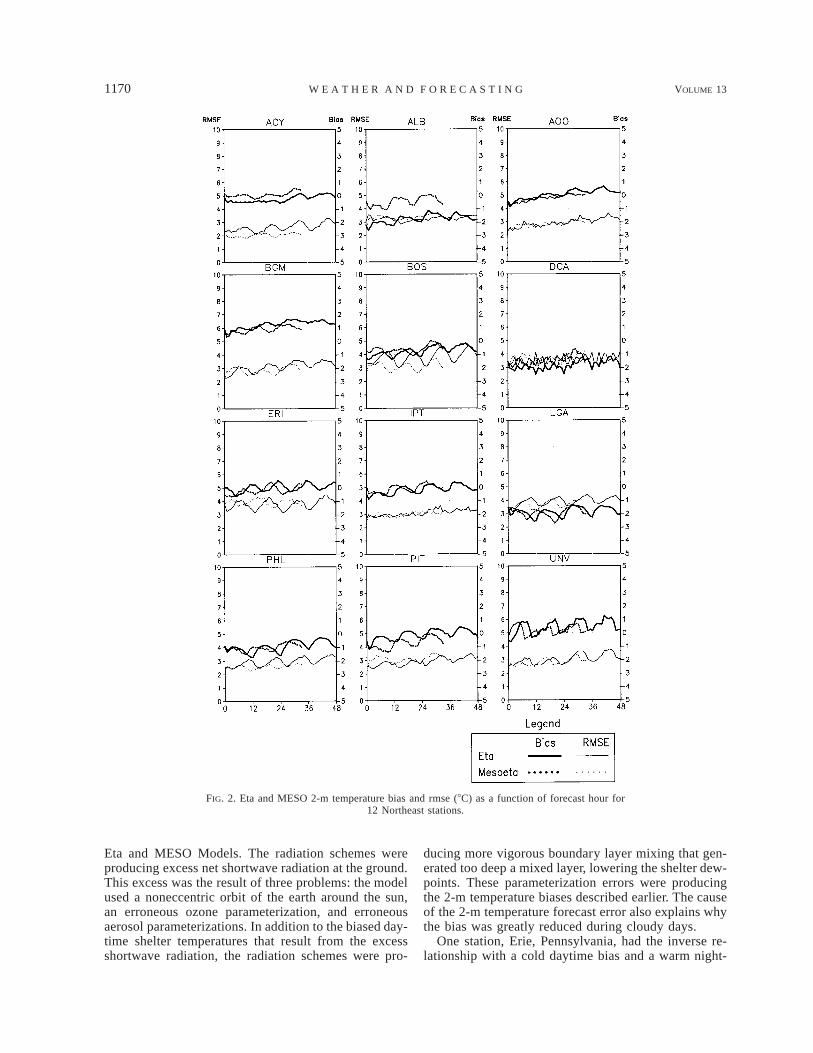
There are significant problems with using the 2-mtemperature as a shelter temperature forecast. Statisticswere compiled for 12 model sounding stations in thenortheast United States on the use of 2-m temperatureas a shelter temperature forecast for a 1-yr period(March 1996–February 1997). These statistics were pro-duced for both the Eta and MESO Models. The NGM

2-m temperature forecast is not provided. Figures 2 and3 present the bias and root-mean-square error (rmse) foreach of the 12 stations for both models. Figure 2 plotsthe statistics as a function of forecast hour, while Fig.3 plots the statistics as a function of time of day.

For 10 of the 12 stations there was a strong cold biasduring the nighttime and a weak to strong warm biasduring the daytime. The cold bias peaked just beforesunrise and the warm bias peaked during maximumheating. The magnitude of the bias at rural locations(Altoona, Pennsylvania; State College, Pennsylvania;and Binghamton, New York) was less than in urbanareas. This suggests that the effects of heat-island in-fluence were contributors. Clearly, however, this cannotbe the sole cause since the bias still exists in rural areas.The bias indicates that the surface radiation and/orboundary layer parameterization schemes may be in er-ror. Another source of the bias would be elevation mis-location between the sounding and station, as previouslymentioned. The largest forecast errors occurred duringtimes of minimal cloud cover. When a clear night wasforecasted, the model 2-m temperature forecast was, onaverage, 38–68C too low. The forecast error was lessduring times of cloud cover and precipitation.

In February 1997 (Table 2), NCEP scientists discov-ered a problem with the radiation schemes within the


FIG. 2. Eta and MESO 2-m temperature bias and rmse (8C) as a function of forecast hour for12 Northeast stations.

Eta and MESO Models. The radiation schemes wereproducing excess net shortwave radiation at the ground.This excess was the result of three problems: the modelused a noneccentric orbit of the earth around the sun,an erroneous ozone parameterization, and erroneousaerosol parameterizations. In addition to the biased day-time shelter temperatures that result from the excessshortwave radiation, the radiation schemes were pro-

ducing more vigorous boundary layer mixing that gen-erated too deep a mixed layer, lowering the shelter dew-points. These parameterization errors were producingthe 2-m temperature biases described earlier. The causeof the 2-m temperature forecast error also explains whythe bias was greatly reduced during cloudy days.

One station, Erie, Pennsylvania, had the inverse re-lationship with a cold daytime bias and a warm night-


FIG. 3. Eta and MESO 2-m temperature bias and rmse (8C) as a function of time of day (UTC)for 12 Northeast stations.

time bias (Fig. 3). The cause of this is the land–oceanmisplacement described previously. The forecast sound-ing for Erie was located over water for both the Eta andMESO Models. Once again, however, it should be notedthat all stations now have corresponding model sound-ing stations that are located over land and thus the biaspresented in Erie and other coastal stations should bediminished. Since these parameterizations have been

fixed, it has been observed that the shelter temperaturesforecast in the model soundings have improved consid-erably. Preliminary poststudy analyses show that the 2-m temperature forecast by the Eta and MESO Modelsnow have a slight to moderate (18–48C) cool daytimebias and a slight (18–28C) nighttime warm bias.

While a discussion of the full ramifications of thislow-level temperature bias is beyond the scope of this


TABLE 4. Optimal threshold low-level relative humidity values forprediction of fog (visibility less than 2 mi) for each of the threemodels. The forecast accuracy at each of these threshold values isalso presented.

Model

Optimal threshold relativehumidity for fog prediction

(visibility # 2 mi)Forecast accuracy

(%)

NGMEta

MESO

959293

666165

paper, it is interesting to note that these biases maycontribute to an increased coastal area baroclinicity. Forexample, in the polar or arctic air mass over land, low-level temperatures are likely to be too cold in the Etaand MESO, especially during the night, as discussedearlier. Over the water, especially the Gulf Stream, thisbias does not exist since the skin temperature is heldfixed to the temperature of the water, thus preventingexcessive radiational cooling as is seen over land duringclear nights with these models. Even over land in thepresence of a tropical air mass, the low-level parame-terized temperature bias is likely to be greatly dimin-ished (compared to that in dry arctic air masses) sincethe moisture content of the boundary layer is excessive.Consequently, these models may artificially enhance thelow-level baroclinicity along the East Coast as a resultof this gradient of low-level temperature bias. This in-creased coastal baroclinicity may lead to an anomalousenhancement of the deepening rates during cyclogene-sis.

b. Experimental fog forecast

The ability of a model to predict fog is directly relatedto its ability to predict low-level moisture. Not all mod-els predict variables explicitly at the surface; therefore,a level close to the surface must be chosen to representthe conditions at the surface. While fog usually occursat relative humidity of close to 100%, model parame-terizations of explicit and convective precipitation gen-eration work feverishly to remove saturation. As a re-sult, it is necessary to determine what forecast subsatu-ration low-level relative humidity can be associated witha prediction of fog. With this question in mind, hourlymodel sounding data were analyzed to determine theability of the profiles to predict fog. The results of thisanalyses are presented in Table 4.

Based on analyses of several hundred forecast hours,it was found that an NGM forecast relative humidity of95% or higher in the lowest sigma layer suggested aforecast of visibility of 2 mi or less. Data were pooledfor 11 cases of synoptically forced fog and low visibilityat Pittsburgh and State College, Pennsylvania, associ-ated with periods of precipitation from September 1995through March 1996. On average, the forecast was cor-rect 66% of the time, on an hourly basis, for all forecasts

out through 48 h. Surprisingly, NGM forecasts validfrom 0 to 12 h in advance were somewhat less accuratethan average, and forecasts for hours 30–42 were some-what more accurate than average. It was apparent thatin many instances the hourly changes in NGM relativehumidity gave indications of the trends toward increas-ing or decreasing visibility. Further, the NGM forecastsdid not always verify observed fog observations on anhour-by-hour basis, but they did show considerable skillin indicating that fog was likely to develop, persist, ordissipate during a period of a few hours through hourlychanges in low-level relative humidity. The NGM hour-ly soundings did not appear to possess significant skillin forecasting localized ground fogs due primarily toradiation.

MESO sounding output for Altoona, Pennsylvania,and Pittsburgh, Pennsylvania, were examined duringMay 1996. Upon examination of three fog events (8days), it was found that the 2-m relative humidity is abetter predictor of fog than is the relative humidity inthe lowest model layer. The 2-m relative humidity wascalculated using the 2-m temperature and 2-m mixingratio. It was determined that the appropriate MESOthreshold forecast relative humidity for a prediction offog of visibility 2 mi or less is 92%. When used, thisforecast was correct 61% of the time, compared to 54%when a relative humidity threshold of 95% was used.The trend of the 2-m relative humidity was often anexcellent indicator of the anticipated breakup or for-mation of fog. Forecast errors were more often due totiming errors than otherwise.

Another indicator of fog breakup or formation wasoften found by comparing the 2-m relative humidity tothe lowest model layer relative humidity. In severalcases, fog formation was associated with a trend inwhich the 2-m relative humidity was increasing fasterthan the lowest model layer humidity. Conversely, fogbreakup was often associated with a trend in which the2-m relative humidity was decreasing more rapidly thanthe relative humidity of the model layer above it. Therewere not sufficient cases of these events to quantify theforecasting ability of this trend.

A similar procedure was applied to the Eta soundingsbetween February and May 1996. Once again, the 2-mrelative humidity was found to be a more accurate in-dicator of fog than the lowest model layer above it. Theoptimal threshold for fog prediction (again, visibility 2mi or less) by this model was found to be 93% (at the2-m level). Forecasts using this threshold were correct65% of the time. Similar to the MESO model, the trendof the fog was often indicated by the trend in the relativehumidity at both the 2-m and lowest model layers. Aswith the NGM soundings, neither the MESO soundingsnor the Eta soundings appeared to have success in pre-dicting ground fogs.

c. Experimental turbulence forecast histogramsThe accuracy of Richardson number forecasts was

examined for the Eta and MESO Models for a period


FIG. 4. Example overlay of forecast Richardson number and pilotobserved turbulence. Analysis of this field was used to evaluate theability of the Eta and MESO Models to forecast CAT. The shadedfield is the forecast Richardson number and the superimposed num-bers are the magnitude of pilot-reported turbulence. An ‘‘3’’ indicatesthat a pilot did not report turbulence.

TABLE 5. Results from the analysis of Eta and MESO forecastingability for pilot-reported turbulence. The period of analysis spans 2weeks at three major airports—New York City’s LaGuardia (LGA),Chicago’s O’Hare (ORD), and Pittsburgh (PIT)—and only includedforecasts of less than 24 h. During this period, 614 turbulent reportswere sent by pilots. In both diagrams, the percentages represent thefraction of the 614 turbulent reports that occurred within a certainwindow of a forecast Richardson number. This window was definedas 28 horizontally, 100 mb vertically, and 3 h temporally. In (a), thepercentages shown are for four independent ranges of Richardsonnumber. (b) Successive cumulative totals of the bins in (a) are rep-resented. For both models, nearly two-thirds of the time a pilot re-ported turbulence the forecast Richardson number was less than 0.25.Nearly 90% of the time turbulence was observed, the forecast Rich-ardson number was less than 1.0.

ForecastRichardson number

Eta forecast vspilot-reported

turbulence (%)

Mesoscale Eta forecastvs pilot-reportedturbulence (%)

(a).1.00.50–1.00.25–0.50,0.25

1413

766

11151064

(b),1.0,0.50,0.25

837366

897464

of 2 weeks (3–16 April 1997) at three major airports(Chicago’s O’Hare, New York City’s LaGuardia, andPittsburgh). This period of time is advantageous in thatit minimizes potential data contamination from convec-tively produced turbulence. Pilot reports (PIREPS) wereexamined and these reports of turbulence were used toverify Richardson number forecasts from the first 24 hof each model forecast. For each station, a pilot reportwas deemed ‘‘at the airport’’ if it occurred within 28lat–long of that airport. Pilot reports of turbulence (withintensity estimates rated 1 to 7, for weak to severe,respectively) were superimposed on model forecastfields of Richardson number, as shown in Fig. 4. If apilot did not report turbulence, an ‘‘3’’ was marked onthe diagram to attempt to validate regions predicting thelack of turbulence. From a model forecast standpoint,turbulence was forecasted as possible when the Rich-ardson number dropped below 1 and probable when itdropped below 0.25. The results of this analysis areshown in Table 5.

Pilot report density played a significant role in ver-ification of turbulence forecasts. Flight occurrences dropoff dramatically after 0100 UTC and remain minimalthrough 1100 UTC. During this time, it was difficult todetermine whether an unverified forecast was the resultof an inaccurate forecast or simply the lack of pilot

reports to verify it. As a result, forecasted turbulenceoccurring during this period was not examined unlessa pilot report was available. Given the large verificationradius for each airport (28), a large verification windowwas applied for each airport. If a pilot report of tur-bulence occurred within 3 h or 100 mb of a forecastedevent, then the report was considered valid for the event.In addition, the 100-mb vertical window was appliedsince Kelvin–Helmholtz wave generation as a result ofclear air turbulence (CAT) may extend above the un-stable layer (as a result of wave breaking or otherwise).

During the 2-week evaluation period, 614 pilot re-ports of turbulence were observed. Of those reports,66% were associated with Eta-based Richardson numberforecasts of less than the empirical critical threshold of0.25. If the constraint on verification is lessened, 73%of the reports occurred with a forecast Richardson num-ber of less than 0.5 and 86% occur with a forecast of1 or less. The ability to forecast turbulence does exist,with nearly two-thirds or more of observed turbulenceevents occurring within the empirically calculatedthreshold.

Determining the false alarm rate of turbulence fore-casts is difficult since the density of pilot reports is low.The vast majority of turbulence reports occur within200 mb of the surface, with a fraction occurring abovethis layer and then mostly at cruising altitudes near jetstreams. The number of pilot reports in the middle tro-posphere (700–400 mb) is low, giving low confidenceto forecasting ability in this region of the atmosphere.Subjectively, it can be said that most of the time whena potentially turbulent layer (Richardson number , 1)


was forecasted above the boundary layer during the 24-h period, a pilot report of turbulence was received. How-ever, using the current observational dataset, the falsealarm rate for predicting turbulence would be excep-tionally high if the lack of a PIREP was used as a neg-ative confirmation since the probability of a thin, short-lived turbulent layer being intercepted by a plane waslow. For this reason, false alarm rate statistics are notbeing presented.

It was observed that model forecasts of boundary layerRichardson number often approach zero (and occasionallydropped slightly below zero during times of superadiabaticlapse rates) and yet turbulence was not reported if theturbulent layer was too shallow. From a verification stand-point, therefore, it is not practical to associate every criticallayer with turbulence since extremely high false alarmrates would result. It is quite evident from this analysisthat a minimal potentially turbulent layer depth is requiredin boundary layer forecasts (and perhaps aloft as well) forturbulence to verify, despite the duration of the unstablelayer. For the three airports evaluated, this critical depthis approximately 75 mb. If this depth was exceeded, pilotreports of turbulence were almost guaranteed if the Rich-ardson number dropped below 0.25. Further, if the poten-tially turbulent layer depth exceeded 150 mb, turbulencewas always reported and often exceeded the rate of fivereports per hour. Additionally, if the turbulent layer depthexceeded 150 mb, the pilot-reported turbulence would fre-quently reach moderate to severe levels (PIREP turbulencelevels 3–7). Yet, if the layer depth dropped near or below75 mb, the number of pilot-reported turbulence eventswould dramatically decrease or vanish. If the depthdropped to or below 50 mb, it was exceedingly rare fora pilot to observe turbulence (even weak turbulence) nearor in the boundary layer, even if the Richardson numberwas near zero for the entire depth of the shallow layer.Given the large number of pilot reports in and just abovethe boundary layer, there is considerable confidence inthese statistics involving critical depth.

Statistics and results from the MESO forecasts aresimilar to those from the Eta forecasts. For the 614 pilot-reported turbulence events, 64% occurred with a Rich-ardson number below 0.25. Further, 74% of the eventsoccurred with a Richardson number of less than 0.5,with 89% occurring with a Richardson number of lessthan 1, as shown in Table 5b. The slightly increasedaccuracy may be due to the increased vertical resolutionof this model; this enables stronger vertical gradients ofwind and temperature, allowing for increased likelihoodthat pilot-reported turbulence would verify in the MESOthan in the Eta Model, where such gradients are slightlyless resolved. Regardless, it appears from this exami-nation that further increases in model vertical resolutionwill not dramatically increase the forecast accuracy ofturbulence, although it may make the forecasts moreprecise. Doing so, however, also raises the potential forfalse alarms, since the areal (vertical and temporal) cov-

erage of the 1.0 value of Richardson number is likelyto increase as vertical resolution increases.

d. Low-level moisture, stratus, and stratocumulusburnoff

During the warm season, a very significant forecastproblem became evident for Pennsylvania and the sur-rounding region: the Eta and MESO Models have ex-treme difficulty in reliably predicting removal of earlymorning low-level stratus and fog. It was quite commonthat the model would predict rapid burnoff of the mois-ture (boundary layer relative humidity dropping below80%), and yet it never occurred, or occurred near sunset.This has severe implications on forecasts of insolation,shelter temperatures, and instability. If the 2-m tem-perature is used as a forecast of shelter temperature, thelargest daytime forecast errors occur between 1700 and2100 UTC (Fig. 3). Of the 10 days with largest forecast2-m temperature error during the spring and summer of1996, 9 of the 10 had overcast skies and fog as weatherconditions. On each of these days, the forecast 2-m tem-perature was off by 108–208C. Such forecast errorswreak havoc on forecasters’ ability to predict the lo-cation and intensity of convection, especially when theenvironment is weakly forced. Is it possible to anticipatedays when stratus and fog will not burn off as quicklyas the model suggests by using forecast boundary layertemperature and moisture profiles?

In an attempt to answer this question, several dozencases were examined during the spring of 1996 in Penn-sylvania where fog and low-level stratus were reluctantto mix out while the Eta and MESO forecasted quickburnoff of the low-level moisture. It appears that in amajority of these cases, this phenomenon can be pre-dicted with reasonable success by examining the verticaland temporal gradients of relative humidity within theboundary layer between 1200 and 1800 UTC. Thesegradients gave clear indications of the degree of mixingthat was likely to occur and whether this mixing wouldbe sufficient to remove the low-level moisture.

Results indicate that on 70% of the days, existinglow-level stratus and fog will not break by 1800 UTCif the following two conditions are met prior to 1800UTC.

1) The forecast maximum relative humidity within theboundary layer (lowest 100 mb) does not drop below80% for two consecutive hours.

2) The forecast shelter (2-m) relative humidity does notdrop below 60% for two consecutive hours.

Two examples of this approach are demonstrated inFigs. 5 and 6. The first example, Fig. 5, demonstratesthe use of the approach to anticipate clearing during themorning hours. Figure 5a is a time–height cross sectionof forecast relative humidity from the 1500 UTC MESOrun of 8 June 1996 for Altoona, Pennsylvania. The periodof interest is from 1200 through 1800 UTC on 9 June.


FIG. 5. Example application of (a) forecast relative humidity time–height cross section to anticipate model forecasterror in (b) low-level temperatures. In this case, forecast 2-m temperatures, shown in (b), had considerable skill inpredicting shelter temperatures during the afternoon of 9 June. The criteria specified in the text are not met in thetime–height cross section of forecast relative humidity shown in (a). Thus, we conclude that sufficient mixing willindeed occur to allow low-level drying and allow forecasters to anticipate that the forecast 2-m temperatures will berealized.


FIG. 6. Example application of forecast relative (a) humidity time–height cross section to anticipate model forecasterror in (b) low-level temperatures. In (a), a forecast cross section of relative humidity is presented from the MesoscaleEta Model for Altoona, PA. The model forecasts deep low-level moisture during the early morning of 8 May, whichdecreases greatly by early afternoon. In (b), the model forecasts 2-m temperatures to rise near 208C by early afternoon.In reality, the observed shelter temperatures remained below 128C the entire day and skies never cleared. By examiningthe temporal and spatial changes in moisture in (a) as described in the text, such a forecast error can be anticipatednearly 70% of the time.


At 1200 UTC the model forecasts a moist boundary layer,which then is mixed vertically through solar heating andthe boundary layer dries to 55% relative humidity by1700 UTC. However, as mentioned earlier, the model isoften too quick in forecasting lowering of boundary layerrelative humidity. Using the approach described above,it can be determined with reasonable accuracy whetherthe low-level relative humidity will, in fact, be decreasedas the model indicates. The first criterion is clearly notmet, since the relative humidity in the boundary layerbetween 1400 and 1800 UTC drops well below 80%.The second criterion is also not met since the shelterrelative humidity drops below 60% at 1600 UTC. Fore-casters should conclude that the model forecast for low-level stratus removal is accurate. The accuracy of theforecast on this occasion can be seen in the shelter tem-peratures. The 2-m forecast temperature (Fig. 5b) was areliable forecast for the shelter temperatures that day,correctly predicting the maximum afternoon temperature,although the timing was off by 3 h.

The second example demonstrates the successful useof the approach to anticipate the maintenance of highboundary layer relative humidity and corresponding cool-er shelter temperatures, avoiding a forecast bust. Figure6a is the forecast relative humidity for Altoona, Penn-sylvania, from the 1500 UTC 7 May 1996 MESO run.The time period of interest is 1200–1800 UTC on 8 May.A saturated boundary layer at 1200 UTC is forecast toremain moist, although below saturation, through 1800UTC. Despite this, the forecast 2-m temperature (Fig. 6b)shows significant warming from 1200 through 1800 UTCduring that day. Forecasters must be skeptical of such ahigh temperature forecast by the model, since the abovetwo criteria are met for this period. Forecasters shouldexpect that the low-level relative humidity will remainhigh, fog and stratus will not dissipate, and that sheltertemperatures are likely to be considerably cooler thanpredicted. Indeed, as shown in Fig. 6b, the observed shel-ter temperatures rose only 48C during the 6-h period,compared to the forecast of a 108–118C rise.

Examination of the 10 events similar to those justdescribed show that on days when the fog and stratusdo not dissipate by 1800 UTC during the spring–earlysummer, a typical daytime maximum temperature isabout 38–88C warmer than the morning minimum. Whenstratus and fog dissipate early, a daytime warmup of98–208C is typical. Thus, the approach just describedcan help forecasters reduce the forecast error of sheltertemperatures during such events.

e. Thunderstorm potential forecasts

For each station available on the Web site, time serieshistograms of storm-relative helicity are provided to theforecaster, along with similar histograms of forecast lift-ed index, total totals index, and K index. Further, all ofthese variables, including convective inhibition, aremade available on the sounding animations. Using these

products, the forecaster can quickly determine the de-gree to which forecast ingredients are coming togetherto yield severe weather at various stations in the forecastarea. The ability of the Eta and MESO to forecast con-vective available potential energy (CAPE), convectiveinhibition (CIN), and helicity—three of the most crucialfactors that determine the thunderstorm potential, type,and severity (Gaza and Bosart 1985; Johns and Doswell1992)—are now examined. The forecasting ability ofthe Eta and MESO was analyzed during 18 convectiveevents in the Pennsylvania and surrounding region dur-ing June and July 1996. During each of these events,the observed soundings at 1200 and 0000 UTC werecompared to forecast model soundings for those times,using the three upper-air sites closest to the Pennsyl-vania region: Pittsburgh, Albany, and WashingtonD.C.’s Dulles International Airport.

1) CAPE FORECASTS

For each of the 18 convective events, the observedand forecast values of CAPE were compared. CAPEwas determined based on the highest equivalent poten-tial temperature layer in the lowest 250 mb at the threesites, which was typically the surface. These observedvalues were then compared to model forecast values ofCAPE for the Eta and MESO Models. Results are shownin Fig. 7. The model forecast values for CAPE werethose from the model run prior to the observation time,giving a 12-h forecast for the Eta Model and a 9-hforecast for the MESO Model. It is acknowledged thatthis analysis is not completely representative of the con-vective potential during these events since the obser-vation times used (0000 and 1200 UTC) are typicallynumerous hours before and after the events occur and,thus, not representative of the convective environmentduring the most unstable time of the day in the UnitedStates. Regardless, this analysis gives a first glance atthe ability of the Eta and MESO Models to predict theseparameters, illuminating any biases that may be presentand applicable to other times during the day whensounding observations are not taken.

In all four diagrams there is considerable spread inthe data, indicating significant difficulty forecastingCAPE. At 0000 UTC, there appears to be slightly greatertendency for each model to overpredict CAPE than tounderpredict it. In those cases where the models over-forecast CAPE, it was typically the result of two factors:(a) forecasting the shelter temperatures too high as aresult of erroneous cloud-cover forecasts described pre-viously or the erroneous radiation parameterization de-scribed previously, and (b) the lack of cool downdraftsin the Betts–Miller convective parameterization scheme,(Black et al. 1993; Black 1994; Janjic 1994), which pro-duces low-level temperature fields that are too warmfollowing convection. The tendency to overpredictCAPE was limited by the models’ tendency to under-forecast afternoon dewpoints by 18–28C during these


FIG. 7. Observed vs forecast CAPE for the Eta and MESO Models.

events. This dewpoint bias is consistent with the biasof overdeepening the boundary layer discussed previ-ously. While the dewpoint has a greater impact on theCAPE calculation, the cool bias associated with the fore-cast dewpoints was considerably less than the warm biasassociated with the forecast temperatures.

It was also noted on several occasions that when el-evated convection was occurring in reality, the Eta andMESO Models had a tendency to underforecast the con-vective response and place the regions of convectiverainfall too far into the low-level high equivalent-po-tential-temperature air. This results from the choice ofconvective parameterization in these models, since thescheme determines cloud base and vertical velocitybased on the lowest 100 mb of the atmosphere, which

can often be quite stable or even exhibit an inversionduring times of elevated convection. In such situations,the scheme would be more likely to produce precipi-tation in the low-level warm air, since the scheme re-sponds more strongly if the unstable air is closer to thesurface. Further discussion and examples of this con-vective bias are given in Grumm and Hart (1998, manu-script submitted to Wea. Forecasting).

At 1200 UTC, the MESO has considerably more skillthan the Eta in predicting CAPE. During the 1200 UTCobservations associated with these 18 events, the largestforecast error for CAPE was 1600 J kg21 by the Eta butonly 600 J kg21 by the MESO. This can be partiallyattributed to the 3-h difference in forecast time betweenthe two models. During several events, it was observed


FIG. 8. Observed vs forecast CIN for the Eta and MESO Models.

that timing errors in frontal passage or advection pat-terns aloft were the cause of erroneous CAPE forecasts,with a few-hour timing error changing CAPE values byone to two orders of magnitude. Based on these resultsand the corresponding discussion, forecasters should notblindly accept forecast values of CAPE. The models doappear to have skill in identifying the high CAPE eventsfrom the low CAPE events, thus alerting the forecasterto the potential of likely thunderstorm type (squall linevs multicell). However, the forecaster should be waryof using the model forecast CAPE to determine the thun-derstorm potential to higher precision, given the models’drawbacks associated with surface temperature forecastsand the lack of cool downdrafts. The short-term fore-casting method advised is to use the model forecast

soundings as a first guess for the current upper- andmidlevel conditions, but to adjust the boundary layertemperature, dewpoint, and wind velocity to those val-ues observed by surface observation stations and theNEXRAD velocity azimuth display (VAD) wind profile.

2) CONVECTIVE INHIBITION (CIN) FORECASTS

Figure 8 illustrates the forecast versus observed con-vective inhibition for each of the 18 convective events.Both models have little skill predicting CIN at 0000UTC if the CIN exceeded 100 J kg21. The occurrencesof underforecasted CIN can be partially attributed to themodels’ tendency to overheat the boundary layer, thuserroneously decreasing the inhibiting factor of warm


FIG. 9. Observed vs forecast environmental helicity (EH) for the Eta and MESO Models.

layers aloft. Again, the bias of underforecasting CINwas limited only by the tendency to underforecast dew-points. In the few cases where the model overforecastconvective inhibition at 0000 UTC, it was the result oferrors in timing of frontal passages. If the model wastoo slow forecasting a cold frontal passage, the CINwould be overestimated; the opposite would be true forforecasts of erroneously early frontal passages.

In contrast to the forecasts valid at 0000 UTC, as thetwo lower panels in Fig. 8 illustrate, the models doappear to possess skill in forecasting CIN during theearly morning (1200 UTC). Both the Eta and MESOappear biased toward underforecasting CIN, though theMESO has a smaller bias. One explanation for the great-er skill at 1200 UTC is that the stable boundary layer

typically found during this time of day makes CIN fore-casting sensitive to the conditions above the boundarylayer. Thus, the CIN field at 1200 UTC is governedmore by the synoptic-scale processes than by the me-soscale or storm-scale phenomena, as may be the caseat 0000 UTC when convection is occurring or has al-ready occurred in the atmosphere or the model. Second,0000 UTC forecasts of surface equivalent potential tem-perature are warm biased (warm surface temperaturebias exceeding cool dewpoint bias), leading to forecastsof CIN that are too low since the temperatures of as-cending parcels are erroneously too warm. Based onthese results, forecasters should be wary of using themodel forecast soundings to anticipate the strength ofconvective inhibition. The intensity of the warm layer


FIG. 10. Observed vs forecast storm-relative helicity (SREH) for the Eta and MESO Models.

aloft producing the inhibition was often correctly mod-eled, but the surface and boundary layer conditions atthe same time were not as well forecasted.

3) ENVIRONMENTAL AND STORM-RELATIVE

HELICITY FORECASTS

During the 18 convective events, the environmentaland storm-relative helicity were calculated for each ob-servation–forecast pair for both the Eta and MESOModels (Figs. 9 and 10). Storm-relative helicity wascalculated using the method described in Davies-Joneset al. (1990). Each model appears to have skill in pre-dicting the environmental helicity at both 0000 and 1200UTC, although there is a slight tendency to overpredict

it. Neither model appears to have significantly more skillthan the other, which can probably be attributed to thehigh vertical resolution of both models. Surprisingly,Fig. 10 indicates that both models have more skill inpredicting storm-relative helicity than environmentalhelicity, with slightly more skill at 1200 UTC than at0000 UTC. However, in many cases during the 2-monthevaluation period storm-relative helicity was increasedon the mesoscale or storm scale due to storm–environ-ment interaction that was not predicted by the model.This mesoscale or storm-scale increase of storm-relativehelicity could be seen on the NEXRAD VAD wind pro-file. Examples of this are discussed in great detail inPearce (1997). The models may provide for a reasonableprediction of the helicity field, but forecasters must be


FIG. 11. (a) Example hourly model sounding-enhanced real-time analysis of CAPE. This particular analysisshows the moderately unstable air to the south of a southward moving cold front. (b) Example hourly modelsounding enhanced real-time analysis of 2-h change in lifted index. Solid contour indicate positive values, while


←

dashed contours indicate negative values. The stabilization of the atmosphere behind the cold front is shown well in this analysis. Two-hourchanges in lifted index of 4–6 exist immediately behind the front. In contrast, the region ahead of the front (Maine, Virginia, and Cape Cod)is continuing to destabilize as shelter temperatures rise.

alert to dramatically increased localized regions of high-er storm-relative helicity resulting from storm–environ-ment interaction (Pearce 1997).

During those days when the environmental or storm-relative helicity was underestimated, it was often dueto the models’ inability to veer boundary layer windssufficiently in the presence of a weak southeasterly flow.Quite often during the evaluation period low-level winds(below 950 mb) would have a slight easterly componentwhile the models would consistently forecast a slightwesterly component. One possible explanation for thiserror is the overheating of the boundary layer previouslydiscussed, which would tend to overmix and overdeepenthe boundary layer depth, erroneously overmixing west-erly momentum closer to the surface and reducing theageostrophic fraction of the total wind at the surface.This 208–408 forecast error in wind direction can dra-matically influence the helicity values. Forecasters mustbe alert to such model forecast errors since such an errorcan create an environment less suitable to mesocyclonedevelopment than the real conditions may indicate. Asnoted previously, the parameterization errors leading tothis bias have been fixed and, thus, we might expectthat the errors in forecast low-level wind velocity shouldbe reduced.

4) CONVECTIVE INITIATION FORECASTS

During weakly forced events, determining the loca-tions and timing of thunderstorm development can beextremely difficult. If the synoptic or mesoscale dynam-ics are weak, determining the location of thunderstormdevelopment hinges on determining the locations wheresurface heating is maximized, surface wind convergenceis increased (through mesoscale, cloud, or topographicboundaries), and convective inhibition is first overcome.The timing of convective initiation (the point at whichconvective development is no longer inhibited by ther-modynamic limitations) is typically given by the pointat which the surface temperature and dewpoint are suf-ficiently high that rising parcels are able to just barelyovercome a layer of CIN.

During the convective season of 1996, the forecastsof convective initiation by the Eta and MESO Modelswere examined, with a focus on weakly forced events.Observed convective initiation was determined whentowering cumulus clouds were first indicated in surfacereports. Model forecast convective initiation was saidto occur when forecast CAPE exceeded forecast CIN.Overall, the results were fair, with convective devel-opment typically occurring within 1–3 h of the modelforecast development (based on CAPE–CIN). There

were, however, numerous cases where timing errorswere significant.

The greatest source of convective initiation timingerror resulted from the tendency of both models to dis-sipate low-level stratus and fog too early, especiallywithin and east of the Appalachian Mountains, as de-scribed previously. If the models removed the low-levelstratus and fog too early, the boundary layer would beforecast to warm too quickly, and the convective tem-perature would be reached too early. This would erro-neously start convection too early and too far east. Inreality, the boundary layer would remain moist andslightly cooler east of the mountains if an easterly com-ponent of the low-level flow existed, while the boundarylayer would warm much more quickly west of the moun-tains. Thus, convection would initiate too late in the eastand too early the west. The tendency to initiate con-vection too early in weakly forced events was also sup-ported by the models’ tendencies to overforecast sheltertemperatures. In cases where the environment wasstrongly forced, errors in convective timing were moreoften the result of erroneous forecast timing of synopticfeatures, such as fronts or jet streaks. Forecasters areadvised to compare observed shelter temperatures toforecast shelter temperatures during the midmorninghours in weakly forced situations to determine if con-vection is likely to be initiated earlier or later than mod-els may indicate.

5) REAL-TIME MODEL SOUNDING ENHANCED

CONVECTIVE ANALYSES

In the United States, upper-air observations are usu-ally taken several hours before and after convectiveevents. For forecasters to estimate convective potentialduring the late morning or early afternoon, morningsoundings are typically adjusted to a forecast surfacetemperature or an observed surface temperature. Thisprocess is fairly limiting, however, since upper-air ob-servations are scarce and, on average, only one obser-vation exists per forecast area. Therefore, mesoscaleforecasting of convective potential is nearly impossibleusing modified observed upper-air soundings. The hour-ly model soundings alleviate, to a large degree, the lim-itations of using observed upper-air soundings. Giventhe hourly resolution, there exists a one-to-one rela-tionship between a forecast model sounding and anhourly surface report. Further, numerous model sound-ings exist within a forecast area, giving the ability todiagnose the convective potential on the mesoscale.

During the convective season of 1997, hourly modelsoundings were used to derive mesoscale analyses of


hourly (real time) convective potential. Approximately50 model soundings were objectively analyzed to pro-duce a three-dimensional grid of forecast thermodynam-ic conditions for each forecast hour. The observed sur-face conditions (temperature and dewpoint) were thenused to determine the lifting condensation level (LCL).Parcel traces from the LCL were then compared to theinterpolated hourly model sounding atmospheric profilefor that forecast hour. Using this method, estimates ofCAPE (Fig. 11a), CIN, and lifted index (Fig. 11b) werecalculated and made available to forecasters through aWeb site (http://hail.met.psu.edu/comet/automet2/automet2.html). In addition, analyses indicating the 2-h changes in these fields were also made available, giv-ing forecasters a sense of the trends in convective po-tential. Finally, standard surface analyses using only sur-face observations were also made available (tempera-ture, dewpoint, equivalent potential temperature, pres-sure change, moisture convergence).

While the synthesis of hourly model soundings andsurface observations alleviates the spatial and temporalresolution problems associated with observed rawin-sonde soundings, it does introduce a larger source oferror. Any model forecast errors will be translated tothe model-enhanced convective fields. This potential forerror is minimized, however, by constantly updating theupper-air objective analysis through use of only the lat-est available set of hourly model soundings. Therefore,typically the upper-air forecast data used in the con-vective fields are no more than 6–9 h old. Forecastersat the National Weather Service Office in State Collegehave expressed a high degree of satisfaction with theconvective analyses. They have found the fields to beuseful in anticipating the formation and dissipation ofthunderstorms, mesoscale convective complexes, con-vective trends, mesoscale boundaries, and areas of mois-ture convergence.

4. Concluding summary and discussion

This research examined the utility of high-resolutionnumerical model vertical profiles to forecast mesoscalephenomena. The vertical profiles were visualized in fourformats: time–height cross sections, time series histo-grams, skew T–logp animations, and distance–heightcross sections. The ability of the NGM, Eta, and MESOModels to forecast warm-season mesoscale phenomenawas examined. The most significant forecast errors werein the forecast shelter-level temperatures, which pro-duced a cascade of impacts on the forecast accuracy ofother mesoscale phenomena, as described below.

The 2-m temperature forecast by the Eta and MESOModels can be used as a forecast for the local surfacehigh and low temperatures. Overall, there exists a warmbias in the 2-m temperature during the daytime and acold bias at night. This bias is maximized during clearskies and light winds. The warm daytime bias also over-deepens the boundary layer, lowering surface dewpoints

too greatly and overmixing westerly momentum to thesurface. Improvements in the model radiation parame-terizations in early 1997 have resulted in a decrease inthe magnitude of the 2-m temperature bias. Preliminaryindications are that a bias still remains, with a slightcold bias (18–48C) during the daytime and a slight warmbias at night (18–28C).

Using the boundary layer relative humidity, theNGM, Eta, and MESO all showed some degree of skillin forecasting fog. The Eta and MESO produced fog atlower empirical relative humidity thresholds than theNGM: 92%, 93%, and 95%, respectively. There waslimited to little skill in predicting localized ground fogs,however. Using the experimental fog product, there didexist skill in forecasting the timing of fog burnoff. How-ever, the Eta and MESO had a tendency to burn off fogtoo quickly in the morning, a consequence of the PBLwarm temperature bias. This tendency to decrease low-level relative humidity too quickly was also seen in themodels’ tendency to remove morning stratus clouds tooquickly. However, by examining the vertical and tem-poral distribution of relative humidity in the boundarylayer, the forecaster is able to overcome the models’fog–stratus removal and associated warm PBL biases.Once this bias was accounted for, skill did exist to fore-cast the removal of early morning stratus.

Modest skill existed in forecasting convection usingthe Eta and MESO Models. The greatest detriments tothe models’ ability to forecast convection were twofold:first, the PBL warm bias produced overestimates ofCAPE and underestimates of CIN. In addition, the in-creased boundary layer depth produced an overmixingof westerly momentum to the surface, which greatlyimpacted helicity forecasts. Second, the Betts–Millerconvective parameterization scheme is not well suitedfor forecasting convection in the middle latitudes. Thescheme is unable to produce cool downdrafts, cannotproduce realistic rainfall rates, and is unable to simulateelevated convection.

The most promising results of this study appeared tobe in forecasting turbulence. The increased accuracy ofthe results may partially be attributed to the relativeindependence of turbulence outside the boundary layerfrom the PBL thermal bias. Forecast Richardson numbervalues of 0.25 or less can be associated with turbulence.Further, values of Richardson number of less than 1 werehighly correlated with a high probability of turbulence.These results show the potential for artificial intelligenceapplications to generate computer-worded aircraft rout-ing forecasts.

Significant spatial errors exist between the Eta–MESO Model sounding location and the observationstation location. The consequences of this displacementcould be seen in forecasts of all warm-season phenom-ena: surface temperature, precipitation, and fog. Theconsequences of this displacement are greatest nearcoastlines and in regions of large terrain gradients. Fu-ture studies involving verification of convective precip-


itation events will likely require interpolation betweenmodel sounding points.

Given the high-resolution and locale-specific fore-casts provided through these model profiles, researchcould be applied to produce artificial intelligence ap-plications that would generate worded forecasts to ac-company the visualization tools shown here. Develop-ment of experimental products during this research wasan integral portion of the success of the project. Usingthese products, forecasters now have nonofficial guid-ance for the occurrence of fog and the threat of tur-bulence to pilots, 1–2 days in advance. These productshave shown variable skill and as forecasters becomemore familiar with the output produced by the products,their utility will only increase with time. However, itshould be emphasized that the criteria found during thisresearch are not necessarily directly applicable to otherregions of the country. Further refinement of empiricalthresholds for other (non-Pennsylvania) locales willlikely be necessary. In addition, the criteria developedduring this research may not perform as well in thefuture as changes to model physics, parameterizations,and resolution occur.

Finally, during the course of this research project,NCEP was provided with the preliminary findings andthey added model sounding sites to expand and improvethe overall study. This led to NCEP’s continued refine-ments and improvements in the parameterizationschemes in the Eta and MESO during the course of thisproject. This interactive relationship facilitated the im-provement of the model profiles’ usefulness and accu-racy as the project continued.

Acknowledgments. The authors gratefully acknowl-edges the support of the National Weather Service andCOMET for supporting this research through a NWS–COMET Fellowship. In particular, funds were providedby the University Corporation for Atmospheric Re-search (UCAR) Subawards UCAR S95-59695 andUCAR S96-75664 and pursuant to the National Oceanicand Atmospheric Administration Awards NA37WD0018-01V and NA57GP0576. The views expressed herein arethose of the authors and do not necessarily reflect theviews of NOAA, its subagencies, or UCAR.

Numerous scientists, students, and forecasters pro-vided invaluable guidance and support during the twoyears of research, without whom this research could nothave been as complete. Keith Brill and Dr. GeoffDiMego of NCEP provided the dataset on which thisresearch was supported. Their efforts to constantly im-prove the quality, completeness, and timeliness of thedataset are greatly appreciated. The efforts to modifythe scope of the dataset to meet the needs of this research

are also appreciated, including the addition of severalmodel sounding stations in the Pennsylvania region. Fi-nally, the authors thank the Center for Ocean–Land–Atmosphere Studies (COLA) of the University of Mary-land for the use of the GrADS software package. Ad-ditionally, we would like to thank Dr. Mike Fiorino ofthe Lawrence Livermore National Laboratory for hishelp with the package during the early stages of thisresearch, including the development of the skew T–logproutine.

REFERENCES

Black, T. L., 1994: The new NMC mesoscale Eta model: Descriptionand forecast examples. Wea. Forecasting, 9, 265–278., D. G. Deaven, and G. DiMego, 1993: The step-mountain etacoordinate model: 80 km early version and objective verifica-tions. NWS Tech. Procedures Bull. 412, 31 pp. [Available fromNational Weather Service, Office of Meteorology, 1325 East–West Highway, Silver Spring, MD 20910.]

Dallavalle, J. P., J. S. Jensenius Jr., and S. A. Gilbert, 1992: NGM-based MOS guidance—The FOUS14/FWC message. NWS Tech.Procedures Bull. 408, 19 pp. [Available from National WeatherService, Office of Meteorology, 1325 East–West Highway, SilverSpring, MD 20910.]

Davies-Jones, R., D. W. Burgess, and M. Foster, 1990: Test of helicityas a tornado forecast parameter. Preprints, 16th Conf. SevereLocal Storms, Kananaskis Park, AB, Canada, Amer. Meteor.Soc., 588–592.

desJardins, M. L., and R. A. Petersen, 1985: GEMPAK: A meteo-rological system for research and education. Preprints, First Confon Interactive Information and Processing Systems, Los An-geles, CA, Amer. Meteor. Soc., 313–319.

Gaza, R. S., and L. F. Bosart, 1985: The Kansas City severe weatherevent of 4 June 1979. Mon. Wea. Rev., 113, 1320–1330.

Hart, R. E., 1997: Forecasting studies using hourly model-generatedsoundings. M.S. thesis, Department of Meteorology, The Penn-sylvania State University, University Park, PA, 166 pp. [Avail-able from Dept. of Meteorology, The Pennsylvania State Uni-versity, 503 Walker Bldg., University Park, PA 16802.]

Hoke, J. E., N. A. Phillips, G. J. DiMego, J. J. Tucillo, and J. Sela,1989: The Regional Analysis and Forecast System of the Na-tional Meteorological Center. Wea. Forecasting, 4, 323–334.

Janjic, Z. I., 1994: The step-mountain eta coordinate model: Furtherdevelopments of the convection, viscous sublayer, and turbu-lence closure schemes. Mon. Wea. Rev., 122, 927–945.

Johns, R. H., and C. A. Doswell III, 1992: Severe local storms fore-casting. Wea. Forecasting, 7, 588–612.

Niziol, T. A., and E. A. Mahoney, 1997: The use of high resolutionhourly soundings for the prediction of lake effect snow. Pre-prints, 13th Int. Conf. on Interactive Information and ProcessingSystems for Meteorology, Oceanography, and Hydrology, LongBeach, CA, Amer. Meteor. Soc., 92–95.

Pearce, M. L., 1997: Non-classic and weakly forced convectiveevents: A forecasting challenge for the dominant form of severeweather in the mid-Atlantic region of the United States. M.S.thesis, Department of Meteorology, The Pennsylvania State Uni-versity, University Park, PA, 122 pp. [Available from Dept. ofMeteorology, The Pennsylvania State University, 503 WalkerBldg., University Park, PA 16802.]

Date post:	07-Nov-2018
Category:	Documents
Upload:	truonglien
View:	213 times
Download:	0 times

The Use of Hourly Model-Generated Soundings to Forecast...

Documents