THE USE OF SERIAL ULTRASOUND EVALUATION OF BODY COMPOSITION TRAITS TO PREDICT PERFORMANCE ENDPOINTS IN COMMERCIAL BEEF CATTLE A Dissertation by SORREL ANN CLEMENT Submitted to the Office of Graduate Studies of Texas A&M University in partial fulfillment of the requirements for the degree of DOCTOR OF PHILOSOPHY August 2009 Major Subject: Animal Science
Transcript
THE USE OF SERIAL ULTRASOUND EVALUATION OF BODY
COMPOSITION TRAITS TO PREDICT PERFORMANCE ENDPOINTS IN
COMMERCIAL BEEF CATTLE
A Dissertation
by
SORREL ANN CLEMENT
Submitted to the Office of Graduate Studies of Texas A&M University
in partial fulfillment of the requirements for the degree of
DOCTOR OF PHILOSOPHY
August 2009
Major Subject: Animal Science
THE USE OF SERIAL ULTRASOUND EVALUATION OF BODY
COMPOSITION TRAITS TO PREDICT PERFORMANCE ENDPOINTS IN
COMMERCIAL BEEF CATTLE
A Dissertation
by
SORREL ANN CLEMENT
Submitted to the Office of Graduate Studies of Texas A&M University
in partial fulfillment of the requirements for the degree of
DOCTOR OF PHILOSOPHY
Approved by:
Chair of Committee, Andy D. Herring Committee Members, Jeff W. Savell
Jason E. Sawyer Tryon A. Wickersham Department Head, Gary R. Acuff
August 2009
Major Subject: Animal Science
iii
ABSTRACT
The Use of Serial Ultrasound Evaluation of Body Composition Traits to Predict
Performance Endpoints in Commercial Beef Cattle. (August 2009)
heifers (n = 172) were evaluated to determine relationships between serial carcass
ultrasound traits and ability to breed in short (45 to 90 d) breeding seasons. Data
collected included carcass ultrasound traits: ribeye area (REA), intramuscular fat
(IMF), rump fat (UFAT), ribfat, weight, and body condition score taken at yearling
age, pregnancy determination, before breeding, and after the breeding season when
pregnancy status was recorded. A logistic regression analysis was used to determine
the influence of ultrasound traits and body condition on pregnancy status. Odds
ratios suggested the likelihood of primiparous cattle rebreeding would have been
increased by 93% if IMF would have averaged 3.5% instead of 2.5% as yearlings, or
an increase in the average ribfat as yearlings from 0.287 to 0.387 cm would have
increased the odds of rebreeding by 88%. Increased average body condition score of
6.5 rather than 5.5 at 30 days postpartum in primiparous cows was estimated to have
increased rebreeding 367%. The odds of yearling Beefmaster heifers successfully
breeding during a 45-day season would have been increased by 73% (year 1) or
iv
274% (year 2) by increasing REA 6.4 to 6.5 cm2 at a year of age. Steers were
serially scanned beginning at approximately 265 kg of body weight through harvest
in 56 day ± 6 intervals. Data collected included ultrasound measurements (ribeye
area (REA), 12th rib fat thickness (RibFat), percent intramuscular fat (IMF), and
rump fat (UFAT)), weight, and carcass data. Days to choice was calculated for each
steer based on a linear regression. The IMF deposition was quantified as quadratic
from scans 1-6 and linear when cattle were on full feed. Prediction models at scans
1, 2, 3, 4, 5, and 6 yielded R-square values of 0.20, 0.25, 0.41, 0.48, 0.59, and 0.49,
respectively for days to choice. Odds ratios suggested that if steers in this study had
averaged 3.78% at day 0 rather than 2.78, the odds of cattle grading premium choice
or greater would have been increased by 300%.
v
ACKNOWLEDGEMENTS
I would not have been blessed so abundantly with the opportunities, sustenance,
or the courage to finish had it not been for the grace of God. Through Him all things
are possible and to Him all praise belongs.
I owe my deepest gratitude to my parents and brothers for their unwavering
support during every step of this project. They organized every data collection
event, managed all the cattle, and funded 100% of this research project.
The pursuit of this degree and completion of this dissertation would not have
been possible without the sponsorship and guidance of Dr. Andy Herring who served
as my major professor and chair. Additionally, without the constant support of Drs.
Jason Sawyer and Tryon Wickersham this dissertation would not be possible. These
three gentlemen always selflessly invested their personal best when asked for
assistance in all aspects of this dissertation as well as my academic career. Their
generosity, vested interest, and support will never be forgotten and they are personal
heroes of mine. I want to acknowledge Dr. Jeff Savell and Dr. Dan Hale for serving
on my committee as members. I would also like to recognize Dr. Michael Speed for
his generous statistical counsel.
I would also like to express my appreciation to Texas A&M University and the
Department of Animal Science to study at a prestigious university and for the
opportunity to complete a doctoral degree.
vi
TABLE OF CONTENTS
Page ABSTRACT ......................................................................................................... iii ACKNOWLEDGEMENTS .................................................................................. v TABLE OF CONTENTS ..................................................................................... vi LIST OF FIGURES ............................................................................................ viii LIST OF TABLES ............................................................................................... ix INTRODUCTION ................................................................................................. 1 Experiment 1 .................................................................................................... 1 Experiment 2 .................................................................................................... 2 LITERATURE REVIEW ...................................................................................... 3 Experiment 1 .................................................................................................... 3 Body composition influences in breeding females .................................. 3 The relationship between body condition score and post- partum interval ......................................................................................... 3 Carcass characteristics and body condition score .................................... 6 Serial carcass ultrasound in breeding females .......................................... 7 Puberty and body composition ................................................................. 9 Carcass ultrasound as a selection tool .................................................... 10
Experiment 2 ................................................................................................. 12 Body composition influences in growing feedlot cattle ........................ 12 The use of parental information to predict carcass merit of progeny .... 13 Deposition of marbling .......................................................................... 14 Using carcass ultrasound to predict carcass composition ..................... 19 Combining ultrasound data and background information ..................... 21 Summary of literature review ................................................................ 21
MATERIALS AND METHODS ........................................................................ 23
LITERATURE CITED ....................................................................................... 64 APPENDIX A ..................................................................................................... 68 APPENDIX B ................................................................................................... 139 VITA ................................................................................................................. 145
viii
LIST OF FIGURES
Page
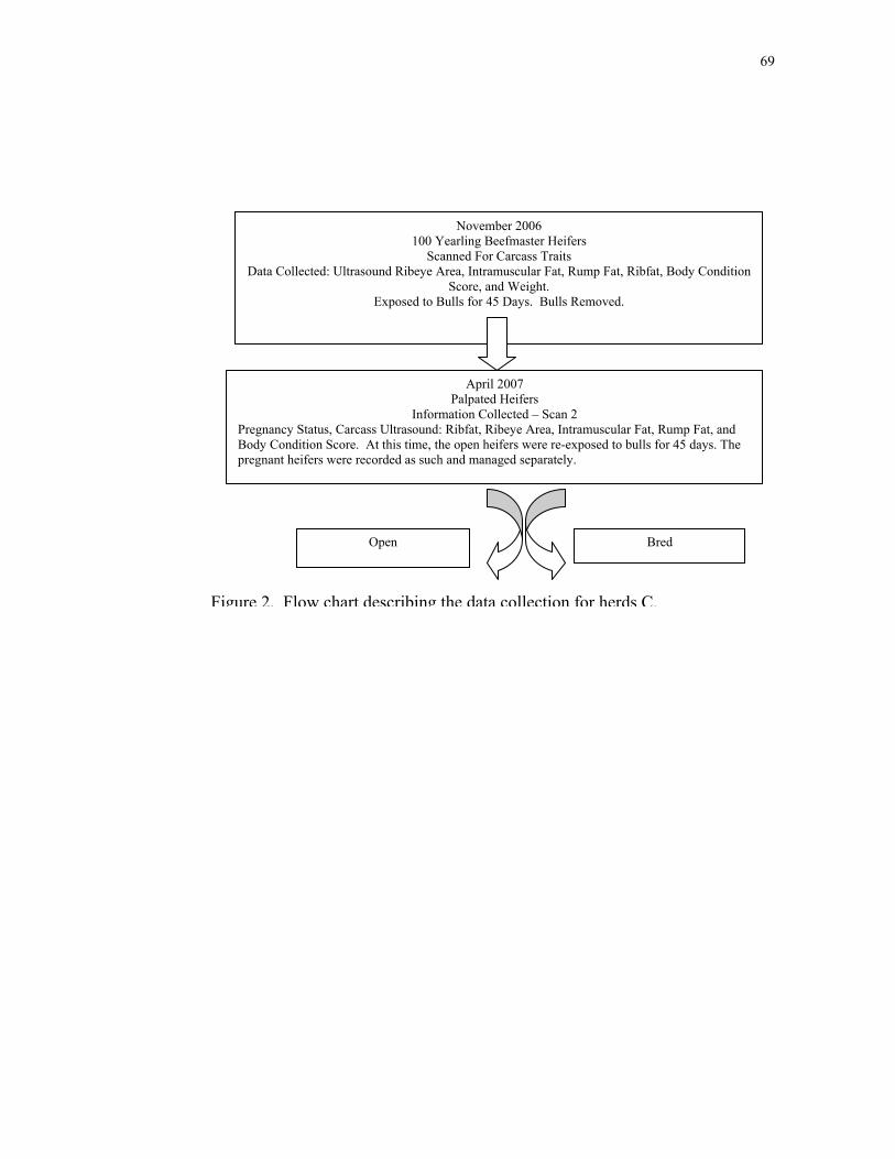
Figure 1. Flow chart describing the data collection for herds A and B .................... 68 Figure 2. Flow chart describing the data collection for herds C .............................. 69 Figure 3. Flow chart describing the data collection for herd D ................................ 70 Figure 4. Representation of least squares means across time for body condition score in herds A, B, and C & D ................................................. 71 Figure 5. Representation of least squares means across time for intramuscular
fat percentage in herds A, B, and C & D ................................................... 72 Figure 6. Representation of least squares means across time for ribeye area
(cm2) in herds A, B, and C & D ................................................................ 73 Figure 7. Representation of least squares means across time for 12th rib fat thickness (cm) in herds A, B, and C & D .................................................. 74 Figure 8. Representation of least squares means across time for fat depth
between the gluteus medias and biceps femoris (cm) in herds A,B, and C& D .......................................................................................... 75
Figure 9. Least squares means estimates plotted across time for weight (kg.) .......................................................................................................... 76 Figure 10.Least squares means estimates plotted across time for ribeye area
(cm2) ......................................................................................................... 76 Figure 11. Least squares means estimates for rib fat across time (cm) .................... 77 Figure 12. Least squares means estimates for IMF across time (%) ......................... 77 Figure 13. Least squares means for UFAT across time (cm) .................................... 78 Figure 14. Least squares means for Intramuscular fat (%) across time by quality grade ............................................................................................. 79
ix
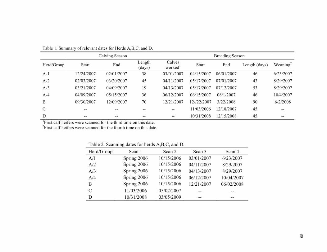
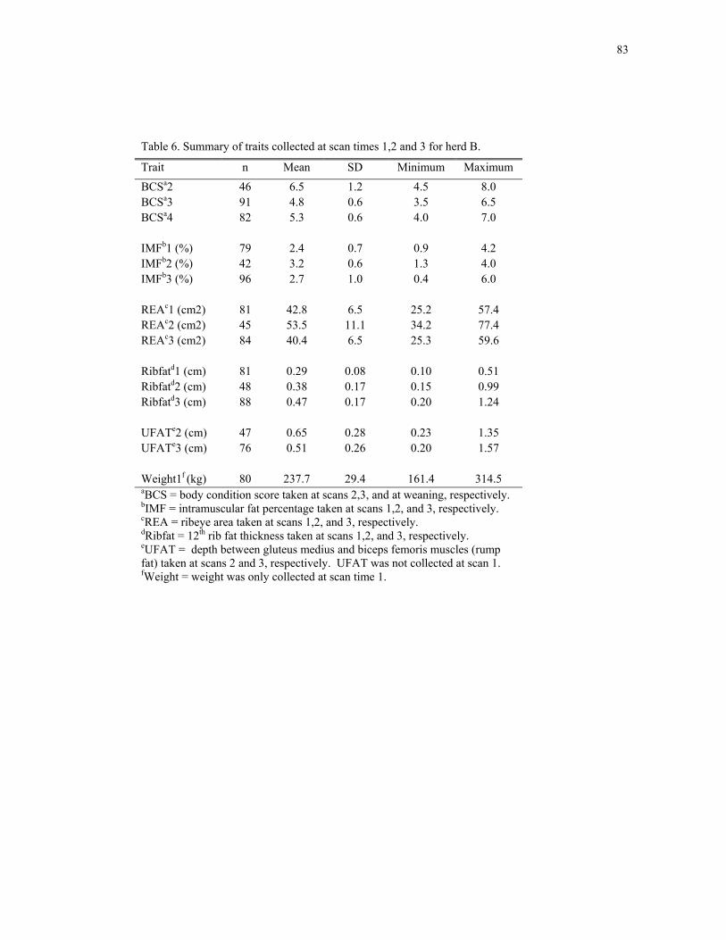
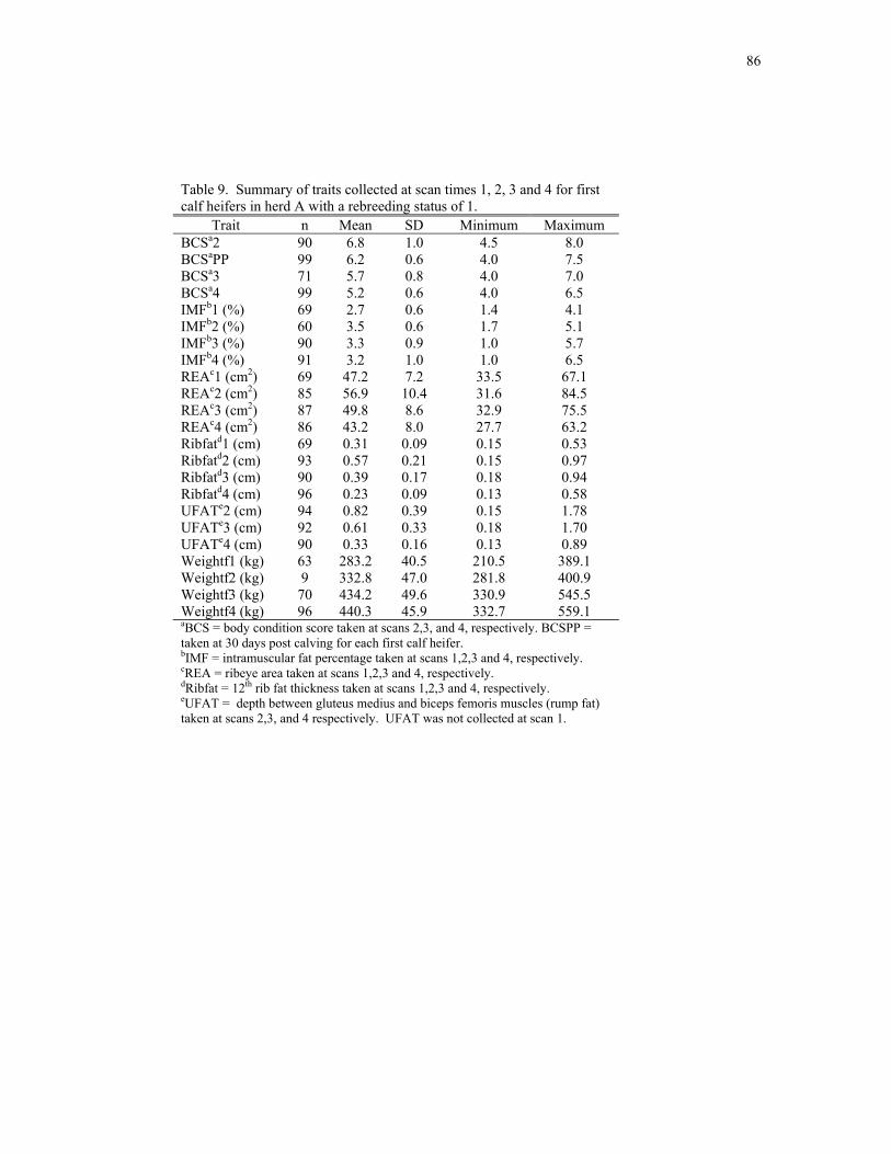
LIST OF TABLES Page Table 1. Summary of relevant dates for Herds A,B,C, and D ..................................... 80 Table 2. Scanning dates for herds A,B,C, and D ........................................................ 80 Table 3. Origin data for steers .................................................................................... 81 Table 4. Serial scan dates and slaughter dates for experiment 2 ................................ 81 Table 5. Summary of traits collected at scan times 1,2,3 and 4 for herd A ................ 82 Table 6. Summary of traits collected at scan times 1,2 and 3 for herd B .................... 83 Table 7. Summary of traits collected at scan times 1 and 2 for herd C ....................... 84 Table 8. Summary of traits collected at scan times 1 and 2 for herd D ..................... 85 Table 9. Summary of traits collected at scan times 1, 2, 3 and 4 for first
calf heifers in herd a with a rebreeding status of 1 ....................................... 86 Table 10. Summary of traits collected at scan times 1, 2, 3 and 4 for first
calf heifers in herd a with a rebreeding status of 0 ...................................... 87 Table 11. Summary of traits collected at scan times 1, 2, and 3 for first
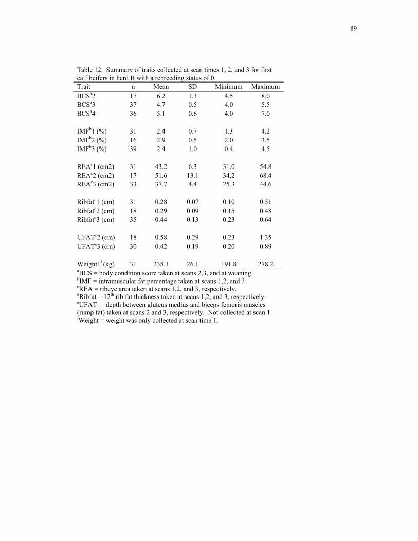
calf heifers in herd B with a rebreeding status of 1 ..................................... 88 Table 12. Summary of traits collected at scan times 1, 2, and 3 for first
calf heifers in herd B with a rebreeding status of 0 .................................. 89 Table 13. Summary of traits collected at scan times 1 and 2 for heifers in
herd C with a pregnancy status of 1 ............................................................ 90 Table 14. Summary of traits collected at scan times 1 and 2 for heifers in
herd C with a pregnancy status of 0 ............................................................ 91 Table 15. Summary of traits collected at scan times 1 and 2 for heifers in
herd D with a pregnancy status of 1 ............................................................ 92 Table 16. Summary of traits collected at scan times 1 and 2 for heifers in
herd D with a pregnancy status of 0 ............................................................ 93
x
Page Table 17. Correlation coefficients, P-values, and number of measurements involving body composition measurements at scans 1-4 in herd A ............................................................................................................. 94 Table 18. Correlation coefficients, P-values, and number of measurements involving body composition measurements at scans 1-3 in herd B ............................................................................................................. 95 Table 19. Correlation coefficients, P-values, and number of measurements involving carcass ultrasound traits measured at scans 1 and 2 for heifers in herd C .................................................................................... 96 Table 20. Correlation coefficients, P-values, and number of measurements involving carcass ultrasound traits measured at scan times 1 and 2 for heifers in herd D ........................................................................... 97 Table 21. Correlation coefficients, P-values, and number of measurements involving carcass ultrasound traits measured at scan 1 in herd A ............................................................................................................. 98 Table 22. Correlation coefficients, P-values, and number of measurements involving carcass ultrasound traits measured at scan 1 in herd B ............................................................................................................. 98 Table 23. Correlation coefficients, P-values, and number of measurements involving carcass ultrasound traits measured at scan 1 in herd C ............. 99 Table 24. Correlation coefficients, P-values, and number of measurements involving carcass ultrasound traits measured at scan 1 in herd D ........... 100 Table 25. Correlation coefficients, P-values, and number of measurements for carcass ultrasound traits measured at scan 2 in herd A .................... 101 Table 26. Correlation coefficients, P-values, and number of measurements involving carcass ultrasound traits measured at scan 2 in herd B .......... 102 Table 27. Correlation coefficients, P-values, and number of measurements involving carcass ultrasound traits measured at scan 2 in herd C for heifers that failed to conceive ........................................................... 103 Table 28. Correlation coefficients, P-values, and number of measurements involving carcass ultrasound traits measured at scan 2 in herd D .......... 104
xi
Page Table 29. Correlation coefficients, P-values, and number of measurements for carcass ultrasound traits measured at scan 3 in herd A .................. 105 Table 30. Correlation coefficients, P-values, and number of measurements involving carcass ultrasound traits measured at scan 3 in herd B ........ 106 Table 31. Correlation coefficients, P-values, and number of measurements for carcass ultrasound traits measured at scan 4 in herd A .................. 107 Table 32. Least squares means for body composition traits across time and rebreeding status in herd A ............................................................ 108 Table 33. Least squares means for body composition traits across time and rebreeding status in herd B ............................................................ 109 Table 34. Least squares means for body composition traits across time and rebreeding status in herds C & D .................................................. 110 Table 35. Effects of ultrasound traits on rebreeding status across evaluation times in herd A ................................................................... 111 Table 36. Effects of ultrasound traits on rebreeding status across evaluation times in herd B .................................................................... 112 Table 37. Effects of ultrasound traits on pregnancy status across evaluation times in herd C .................................................................... 113 Table 38. Effects of ultrasound traits on pregnancy status across evaluation times in herd D ................................................................... 114 Table 39. Effects of body condition rebreeding status across evaluation times in herd A ................................................................... 115 Table 40. Effects of body condition on rebreeding status across evaluation times in herd B .................................................................... 116 Table 41. Effects of body condition score on pregnancy status across evaluation times in herd C .................................................................... 117 Table 42. Effects of body condition score on pregnancy status across evaluation times in herd D ................................................................... 117
xii
Page Table 43. Summary of real time ultrasound traits and weights taken at scan times 1-6 ....................................................................................... 118 Table 44. Summary of carcass traits .................................................................... 119 Table 45. Correlation coefficients, P-values, and number of measurements involving real time ultrasound measures of IMF at scan times 1-6 and carcass marbling score ............................................................ 120 Table 46. Correlation coefficients, P-values, and number of measurements involving real time ultrasound measures of REA at scan times 1-6 and carcass ribeye area ................................................................... 121 Table 47. Correlation coefficients, P-values, and number of measurements involving real time ultrasound measures of Ribfat at scan times 1-6 and carcass back fat ...................................................................... 122 Table 48. Correlation coefficients, P-values, and number of measurements involving real time ultrasound measures of weight at scan times 1-6 and hot carcass weight .................................................................. 123 Table 49. Correlation coefficients, P-values, and number of measurements involving real time ultrasound measures of UFAT at scan times 1-6 ......................................................................................................... 124 Table 50. Correlation coefficients, P-values, and number of measurements involving real time ultrasound traits at scan time 1 ............................ 125 Table 51. Correlation coefficients, P-values, and number of measurements involving real time ultrasound traits at scan time 2 ............................. 126 Table 52. Correlation coefficients, P-values, and number of measurements involving utrasound traits measured at scan 3 ..................................... 127 Table 53. Correlation coefficients, P-values, and number of measurements involving ultrasound traits measured at scan 4 ................................... 128 Table 54. Correlation coefficients, P-values, and number of measurements involving ultrasound traits measured at scan 5 .................................... 129 Table 55. Correlation coefficients, P-values, and number of measurements involving ultrasound traits measured at scan 6 .................................... 130
xiii
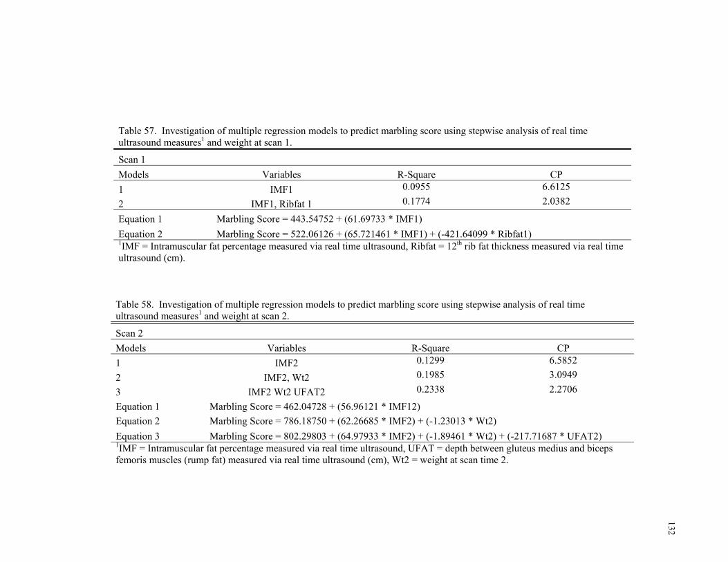
Page Table 56. Correlation coefficients, P-values, and number of measurements involving carcass data ........................................................................... 131 Table 57. Investigation of multiple regression models to predict marbling score using stepwise analysis of real time ultrasound measures and weight at scan 1 ................................................................................ 132 Table 58. Investigation of multiple regression models to predict marbling score using stepwise analysis of real time ultrasound measures and weight at scan 2 ............................................................................... 132 Table 59. Investigation of multiple regression models to predict marbling score using stepwise analysis of real time ultrasound measures and weight at scan 3 ............................................................................... 133 Table 60. Investigation of multiple regression models to predict marbling score using stepwise analysis of real time ultrasound measures and weight at scan 4 ............................................................................... 133 Table 61. Investigation of multiple regression models to predict marbling score using stepwise analysis of real time ultrasound measures and weight at scan 5 ............................................................................... 134 Table 62. Investigation of multiple regression models to predict marbling score using stepwise analysis of real time ultrasound measures and weight at scan 6 ............................................................................... 134 Table 63. Investigation of multiple regression models to predict days to choice using stepwise analysis of real time ultrasound measures and weight at scan 1 ............................................................................... 135 Table 64. Investigation of multiple regression models to predict days to choice using stepwise analysis of real time ultrasound measures and weight at scan 2 ............................................................................... 135 Table 65. Investigation of multiple regression models to predict days to choice using stepwise analysis of real time ultrasound measures and weight at scan 3 ............................................................................... 136
xiv
Page Table 66. Investigation of multiple regression models to predict days to choice using stepwise analysis of real time ultrasound measures and weight at scan 4 ............................................................................... 136 Table 67. Investigation of multiple regression models to predict days to choice using stepwise analysis of real time ultrasound measures and weight at scan 5 ............................................................................... 137 Table 68. Investigation of multiple regression models to predict days to choice using stepwise analysis of real time ultrasound measures and weight at scan 6 ............................................................................... 137 Table 69. Effects of ultrasound and animal body composition traits on attaining marbling score 600 or greater across time............................... 138
1
INTRODUCTION
The value of carcass ultrasound, or any tool used to make predictions, is the
ability to identify and adjust management strategies early in the production phase to
optimize an animal’s performance. This study is divided into two experiments which
explore serial ultrasound as a means to make predictions about reproductive
performance and feedlot performance of commercial cattle.
Experiment 1
Maternal productivity (defined for the purpose of this paper as the ability of a
primiparous heifer to calve as a two year old, breed back in less than 80 days post
partum so as to maintain a 365 day calving interval, and wean a healthy calf) is
extremely influential upon profit, but is hard to predict as it is influenced by many
factors. In commercial heifers, visual characteristics are the primary assessment of
maternal productivity potential as a result of lack of records in most cases. If
maternal productivity could be predicted at a younger age, heifers could be sorted
into groups based on predicted maternal abilities and managed or culled accordingly.
Thus, one of the purposes of this study is to explore ultrasound measures of body
composition as a means to evaluate potential maternal productivity in yearling
heifers.
The research objectives that defined Experiment 1 were to 1) study
relationships between maternal productivity and ultrasound body composition
__________________ This dissertation follows the style and format of the Journal of Animal Science.
2
measures in commercial females, and 2) establish ultrasound carcass data thresholds
which accurately predict maternal performance in yearling heifers.
Experiment 2
With pressure from rising input costs and increased cost of gain, the
implementation of tools that boost efficiency within feeding programs for beef cattle
are prevalent, and should continue to be explored in depth. Real time ultrasound has
the ability to increase efficiency within the feeding sector in terms of nutritional
management, sorting, and marketing. While the identification of cattle that do not fit
a certain market prior to exposure of discounts is desirable, a greater advantage
would be earlier identification of those cattle, maximizing the opportunity to
implement management strategies that favored increased efficiency through targeted
feeding programs.
The research objective that defined Experiment 2 was to establish the period
in a calf’s life from weaning to harvest when accumulation of fat, specifically
intramuscular fat, is most correlated to the end carcass quality grade that could be of
future use for sorting cattle.
3
LITERATURE REVIEW
Experiment 1
Body Composition Influences in Breeding Females
Strong evidence exists that body composition plays a vital role in the
regulation of estrous in beef cattle. This portion of the literature review attempts to
capture the significance of the relationship between body composition and post
partum interval, explore research on the relationship between body composition
measures and carcass traits, and investigate the potential relationships between
carcass traits and maternal ability. Published literature from experiments where
carcass ultrasound was used in heifers or cows is also presented here.
The Relationship between Body Condition Score and Postpartum Interval
Immediately following parturition, a critical period of 80 days exists in which
a cow must breed back to maintain a 365 day calving interval. Therefore, if two
opportunities are to be presented for breeding, cows must be cycling by day 60
postpartum (Dunn and Moss, 1992). Previous research has been conclusive in that
post partum interval is a dynamic trait affected by a variety of factors including
season, suckling, forage conditions, nutritional stress, and age (Wetteman et al.,
1986; Short et al., 1990; Randel, 1990; Dunn and Moss, 1992; Hess et al., 2005), but
is mostly highly influenced by body condition, which reflects the sum of all three
factors.
Body energy reserves at calving are the most influential factor on length of
post partum interval according to Wettemann et al. (1986). Dunn and Moss (1992)
4
emphasized an animal’s ability to repartition nutrients, and this phenomenon’s effect
on reproduction. Mammals cannot perform for any extended period of time in a
deficient state of any required nutrient. When the net energy of an animal’s diet is
significantly less than the energy expenditure of the animal; the result is a negative
energy balance. Cows are able to repartition nutrients for physiological functions
only if they have sufficient nutrients to meet their fundamental necessities which are
prioritized in an inherent order essential to life; 1) basal metabolism, 2) activity, 3)
growth, 4) basic energy reserves, 5) pregnancy, 6) lactation, 7) additional energy
reserves, 8) estrous cycles and initiation of pregnancy, and 9) excess reserves (Short
et al., 1990). Since reproduction is not essential to the survival of the individual
animal, it is usually subordinate to those processes essential to life (basal metabolic
rate, activity or growth). Randel (1990) found that underfed lactating cows have
extended periods of ovarian inactivity which supports this theory of repartitioning.
The effects of nutrition upon reproduction depend upon a web of variables
including nutritional content of feed, body condition of the cow, and other
physiological functions such as lactation or growth. For example, growth in first calf
heifers is an existing priority that takes precedence over reproduction thus reflecting
the root of the common dilemma in achieving rebreeding success in first calf heifers
(Short et al., 1990).
Body condition score (BCS), a subjective, visually assessed trait, is defined
by degree of fat cover on an individual. The most commonly used scale is 1 to 9,
with 1 representing the state of emancipation and 9 representing obesity (Wagner et
5
al., 1988). Body condition score has been used with a high degree of accuracy to
identify heifers and cows that will breed back at a faster rate (Corah et al., 1975;
Dunn and Moss, 1992; DeRouen et al., 1994; Spitzer et al., 1995; Ciccioli et al.,
2003.)
Cows experience an increased nutritional demand during the last trimester of
gestation and in early lactation. Consequently, it is vital for most cows to calve in a
body condition score of 5 to 6 and maintain that condition to account for the
nutritional demands experienced post parturition (Spitzer et al., 1995; Ciccioli et al.,
2003; Lake et al., 2007). DeRouen et al. (1994) reported that pre-partum body
weight and condition fluctuations had less influence on reproductive performance
than body condition at calving given that management conditions remain consistent
after calving. A study by Ciccioli et al. (2003) showed that cows must be managed
to maintain or increase body condition during lactation if expected to breed back in
80 days postpartum. This study also confirmed that cows fed to maintain or lose
body condition during lactation have prolonged intervals from calving to estrus, are
less fertile, and wean lighter calves (Ciccioli et al., 2003).
In studies that investigated post-calving supplemental effects Dunn et al.
(1969) found that the pregnancy rate 120 days postcalving was directly related to
post calving energy level in Angus and Hereford primiparous heifers. In the study,
cows were fed a low-low, low-moderate, high-low, and high-moderate or high-high
supplemental plane of nutrition pre-calving and post-calving for 60 days and then
challenged to rebreed in a 60 day breeding season. Post partum interval was longer
6
for cattle on a low pre-calving plane of nutrition, and the study concluded that pre-
calving nutrition effects the first 100 days of post-calving estrous regulation, and low
levels of nutrition pre-calving cannot be overcome by compensation through
excessive supplementation post-calving (Dunn et al., 1969).
In summary, body condition score immediately prior to and during the
breeding is critical. Body condition score should be managed so that cows have
sufficient reserves to calve, lactate, and maintain an adequate amount of condition
during the breeding season. Body condition score at calving is a good indicator of
body condition score at breeding if cattle are managed to account for the increased
nutritional demands that parturition and lactation present. Although a body
condition score of 5-6 has been recommended in previous literature, it should be
noted that this “optimum” condition score is based on achieving the shortest post
partum interval.
Carcass Characteristics and Body Condition Score
It has been demonstrated that body condition score is highly related to
reproductive performance and calf weaning weight. Bullock et al. (1991) and Apple
et al. (1999) attempted to define the relationship between carcass traits and BCS in
commercial cows. A study completed by Apple et al. (1999) was conducted with 83
mature culled beef cows of British influence 6 to 8 years of age, which were
assigned BCS prior to slaughter. Cattle were sorted into body condition scores that
ranged from 1 to 8. At slaughter, the carcasses of cows assigned BCS scores of 8,
prior to slaughter, exhibited the most marbling. The percentage of carcasses grading
7
U.S. utility or higher was 16.7%, 20.0%, 63.6%, 43.3%, 73.3%, and 100.0% for
cows assigned a BCS of 2, 3, 4, 5, 6, 7, and 8, respectively (Apple et al., 1999).
Bullock et al. (1991) evaluated the relationship between body condition and
carcass traits on 39 Angus x Hereford cows aged from 3 to 10 years, which were
sorted into three body condition groups based on ultrasonic measurements. One cow
from each group was slaughtered for an initial benchmark representation from each
body condition group. The remaining females were sorted into two sub groups; one
fed to gain and one fed to lose weight. Two cows from each group were slaughtered
to evaluate effects of nutrition. The correlation between BCS and marbling was 0.86
indicating that BCS can be used to predict marbling in mature cows (Bullock et al.,
1991). Lake et al. (2007) found that among three-year-old Angus x Gelbvieh heifers
managed to calve with body condition score of 4 had lower ultrasonic 12th rib fat at
day 3 of lactation when compared to cattle that were managed to calve in a BCS of 6.
Additionally, BCS was correlated with 12th rib fat at a correlation of r = 0.87 and
with body weight at a correlation of r = 0.75 on day three of lactation (Lake et al.,
2007).
Serial Carcass Ultrasound in Breeding Females
Rouse et al. (2001) used ultrasound to determine the changes in carcass
composition with regard to the stresses of calving, lactation, and rebreeding in first
calf Angus heifers. Body condition score and pregnancy data were not collected.
Angus heifers were scanned for carcass traits five times: (1) before breeding, (2)
before first calving, (3) at weaning of first calf, (4) before second calving, and (5) at
8
weaning of second calf. Ribeye area increased linearly throughout the five scans in
the study by Rouse et al. (2001), but the linear trend was not observed in this study in
either herds A and B. Weight increased until calving, whereupon heifers lost an
average of 38 kilograms during the first 183 days of lactation, and then resumed
weight gain (Rouse et al., 2001). It should be noted that the postpartum weight loss
did include fetal and placental weight. The pattern for subcutaneous fat followed
that of body weight changes with values of 0.08, 0.16, 0.14, 0.24, and 0.29 inches for
scans 1 through 5, respectively (Rouse et al., 2001). The intramuscular fat
percentage measurements took longer to recover than subcutaneous fat levels
although both traits followed the same pattern. This same pattern was observed in
herds A and B. Mean values of intramuscular fat percentages were 4.95, 5.13, 4.53,
4.11, and 5.11 for scans 1 through 5, respectively (Rouse et al., 2001). While
subcutaneous fat levels began to recover after weaning of the first calf, intramuscular
fat percentage did not begin to increase until weaning of the second calf (Rouse et
al., 2001). Two groups of heifers (n = 72 and n = 41), within the sample studied, did
not deviate from the general trend of sample means for intramuscular fat percentage
changes, but the rate of change differed by more than two percentage points from the
sample means, and less than one percentage point from the sample means,
respectively (Rouse et al., 2001).
The majority of research on post partum interval in primiparous heifers has
been done using BCS as a measurement tool because it is conveniently assessed, and
is highly related to fertility. Body condition can be used to identify which cows
9
should rebreed in a timely manner. However, some cows will rebreed at lower BCS
than recommended, and some will require more condition to conceive. It would be
valuable to determine which heifers have greater chances for maternal productivity
as yearlings, so efficiency in management could be improved prior to breeding. If
body condition in first calf heifers is correlated to ultrasound carcass data, the
potential of prediction, by means of ultrasound, of yearling heifers that have the
potential to excel in maternal productivity could be greatly increased. Due to
research that indicates maternal physiological processes influence body fat
composition including intramuscular and subcutaneous fat depots, the potential for
using these depots to predict maternal performance in yearling heifers exists.
Puberty and Body Composition
The ability of heifers to breed early in the breeding season is indicative of
their overall lifetime performance in terms of calves and pounds weaned (Lesmeister
et al., 1973). In a study consisting of 481 cows and 2,036 subsequent calves,
Lesmesier et al. (1973) found that not only did heifers that bred earlier in the season
continue to breed back early in succeeding breeding seasons, but calves born to these
females had an advantage in average daily gain from birth through finish compared
to later born contemporaries.
The initiation of puberty is characterized by the regulation of the GnRH
regulator (Ojeda et al., 2006). There are many factors that can limit puberty in
heifers such as nutrition (Hall et al., 1995), breed (Baker et. al, 1988), and season
(Schillo et al., 1992). Hopper et al. (1993) found that when comparing Angus to
10
Santa Gertrudis heifers, Angus heifers were fatter at puberty and physiologically
older at the same chronological age. This is most likely due to the puberty
differences for breed type as found by Baker et al. (1988) who found that Bos indicus
cattle are heavier, taller, and older at puberty. However, it seems that earlier
maturing breeds like Angus have greater amounts of fat in reserves for times of
nutritional stress such as gestation and lactation thereby having a better chance to be
in a suitable body condition to breed back at these times (Hopper et al., 1993).
Wiltbank et al. (1985) found that heifers that were managed to achieve 318
kg at the initial breeding season conceived 20 days earlier in the breeding season
than heifers managed to weigh 272 kg. Cattle were ½ to ¼ Brahman and the same
trend was evident in the subsequent year’s breeding season (Wiltbank et al., 1985).
Carcass Ultrasound as a Selection Tool
Little research has been done in terms of predicting maternal productivity in
heifers using carcass ultrasound. With the low heritability of reproductive traits
(heritability of pregnancy and first conception was found to be 0.13 ± 0.07 and 0.03
± -0.03, respectively, by Minick et al. (2001) with data from six herds in 5 states
with a population of 3,144 head of cattle), ultrasound offers potential as a tool for
selection. More research is needed to determine if carcass ultrasound data can
indeed be used to predict maternal performance of yearling heifers.
In a study conducted on Angus cattle, Minick et al. (2001) found that heavier
yearling heifers were more likely to possess mature reproductive tracts at breeding
than their lighter weight contemporaries. Additionally, heavier heifers exhibited
11
larger ribeyes, more rump fat at one year of age, and were more likely to be cycling
at one year of age. Heifers were scanned at 268, 303, 370 and 405 days of age
(Minick et al., 2001). Patterson et al. (1992) showed similar findings in that heifers
that weighed more at weaning were more likely to reach puberty earlier than their
contemporaries in a study comparing Brahman x Herefords (n = 148) to Angus x
Hereford (n = 148) heifers. The earlier maturing Angus x Hereford heifers produced
heavier calves, but had a longer post partum interval (Patterson et al, 1992).
However, this relationship was not exhibited in the Brahman x Hereford heifers
(Patterson et al, 1992). It should also be noted that earlier maturing heifers in the
study weaned heavier calves and consequently had decreased body condition scores
at breeding which may be partly responsible for the longer post partum intervals
(Patterson et al, 1992).
Until one year of age, heifers are typically managed as a single group, and so
carcass data prior to one year of age is beneficial. Once exposed to bulls for the first
time, variables such as pregnancy and cycling status emerge which heighten the
opportunity for division of herd into management groups for efficiency purposes.
After breeding, it becomes more economical to manage heifers based on their
physiological needs. If a relationship between scanned carcass data taken at one year
of age and maternal productivity exists, the potential to identify and sort heifers
based on physiological potential, management needs, and predicted performance
would also exist.
12
Wilson et al. (2001) found that in Angus, the heritability estimates from
developing heifer carcass data were higher than those estimated from yearling bull
data and thus more accurate in predicting carcass merit of steer-mate half-sibs.
Perhaps this is due to the fact that carcass composition is more similar between
yearling heifers and yearling steers than that of yearling bulls and yearling steers, or
the fact that there is less variation among bulls than heifers when scanning took
place. This finding shows a promising future for the continued research on carcass
data of commercial females and their subsequent maternal performance and carcass
merit of their offspring.
If scanned carcass data taken at one year of age could predict performance
with regard to post partum interval and the carcass merit potential of her offspring,
time and money could be saved. Additionally, heifers could be matched with bulls
that complement the carcass merit profile of the female to produce more
predictability in carcasses of offspring.
Experiment 2
Body Composition Influences in Growing Feedlot Cattle
The development of body composition measurements, especially
intramuscular fat, has been studied with both serial slaughter and serial ultrasound in
the past. Previous research indicates that body compositional changes in growing
cattle are influenced by a variety of factors of both genetic and environmental
origins. This portion of the literature review will present research that pertains to the
relationship between carcass traits in growing beef cattle.
13
The Use of Parental Information to Predict Carcass Merit of Progeny
Relative variances in carcass traits measured via ultrasound have been proven
to be passed to progeny through the additive genetic component. Heritability (the
fraction of total phenotypic variation due to variation in breeding value differences)
of carcass traits are moderately heritable with values reported by Kemp et al., (2002)
as 0.36, 0.39, 040, 0.17, 0.38, and 0.49 for carcass ribeye area, carcass fat thickness,
increased accuracy in prediction models where additional information was known
such as sire, ultrasound information, and ranch of origin (Dean et al., 2006). All
cattle had information pertaining to weight, muscle and frame score, and ultrasound
measures. However, only a portion of the cattle had known sires. The results
indicated that percentage of variation accounted for was greater in cattle with
additional pieces of information such as known sire. Ultrasound information was
used to a greater potential when used in combination with other pieces of
information that accounted for variation in carcass traits such as sire and ranch of
origin. This study indicated the potential value of additional calf background
information in combination with ultrasound measurements for increased
predictability of profit on a per animal basis.
Summary of Literature Review
As extensive research supports, body condition score has been a reliable
indicator of reproductive performance in beef cattle and regulation of the estrous
22
cycle. Limited research has been published on the relationship between either body
condition score or reproductive performance and carcass ultrasound traits. The
purpose of this study was to explore ultrasound measures of body composition as a
means to evaluate potential maternal productivity in yearling heifers. The research
objectives that defined Experiment 1 were to 1) study relationships between maternal
productivity and ultrasound body composition measures in commercial females, and
2) establish ultrasound carcass data thresholds which accurately predict maternal
performance in yearling heifers.
Research pertaining to changes in body composition as expressed through
serial slaughter and serial ultrasound in growing beef calves have been summarized
in this paper. Marbling deposition occurs consistently throughout a calf’s life and
has been shown to be linear when expressed as a function of hot carcass weight. The
research objective that defined Experiment 2 was to establish the period in a calf’s
life from weaning to harvest when accumulation of fat, specifically intramuscular fat,
is most correlated to the end carcass quality grade that could be of future use for
sorting cattle.
23
MATERIALS AND METHODS
This project was organized as two distinct, but related experiments.
Originally, the calves from Experiment 1 were to be used in Experiment 2.
However, due to unforeseen management issues, only 25% of the calves were
retained for the project, and the other 75% of the calves in Experiment 2 came from
outside sources. Body composition measures in breeding females were evaluated via
ultrasound, body condition score evaluation, and weight before and after the
breeding season in both first calf heifers and primiparous heifers. This component is
referred to as Experiment 1. Ultrasound measures of body composition as well as
weight were also investigated in growing steers to every 56 days from
preconditioning to slaughter. This component is referred to as Experiment 2. Both
experiments were designed to investigate the efficacy of using carcass ultrasound to
sort cattle based on a desired endpoint. The desired endpoints were pregnancy and
quality grade in experiments 1 and 2, respectively.
Experiment 1
Cattle
There were four experimental groups of cattle upon which data were
collected, all of which were privately owned cattle in cooperator herds. The groups
differed in breed composition, calving dates, calving locations, or age, as illustrated
in Tables 1 and 2. Herds A and B were F1 Brahman x Hereford heifers (n = 412)
ranging in age from 9 to 15 months when acquired from Nixon and Poteet, Texas
and transported to Parker County Texas. Cattle that did not breed during the initial
24
90 day breeding season were exposed to bulls for an additional 90 days before they
were culled from the experiment. This would have been the first breeding season for
these heifers. It is important to note, that although heifers arrived in a group with a
spread of an estimated 6-month range in age, only heifers that calved as 2-yr-olds
were utilized for this project. Cattle were divided into a spring (herd A) and fall
(herd B) calving groups, and these were analyzed separately. The management and
data collection schedules for these two herds are shown in Figure 1. Herd A was
divided into four groups to account for seasonal variations in the weather and forage
supply since the calving season spanned January to May. Group 1 through 4 in herd
A had approximately 50 calves each and included heifers that calved within 45 days.
Herd B was managed as a single group. The breeding performance trait accessed
was the ability for the first calf heifer to rebreed in the postpartum breeding season of
45 or 90 days, respectively, for herds A and B. Additionally, two sets of yearling
heifers, herds C and D, were evaluated for the same aforementioned traits prior to
and after the initial breeding season, as shown in Figures 2 and 3, respectively.
Breed composition of these heifers was Beefmaster (n = 100 and n = 72 for herds C
and D, respectively). The performance trait accessed for herds C and D was
pregnancy status as a result of the initial 45 day breeding season. Herds C and D
were both managed on a single ranch in Shackelford County, Texas, during two
management seasons (2006 - 2007 and 2008 - 2009). A summary of calving and
weaning dates across these herds is provided in Table 1.
25
Cows in herd A were challenged to rebreed for the first postpartum breeding
season in 45 days; cows in herd B were challenged to rebreed for the postpartum
breeding season in 90 days. Cattle in herds C and D were challenged to breed at 14
months during an initial 45 day breeding season. Cattle that were determined as
pregnant were designated to have a pregnancy status of 1, and cows that were
determined not pregnant were designated as 0. For herds A and B this represented
rebreeding status after their second breeding season, whereas for Herds C and D, this
represented pregnancy status following their first breeding season.
Data Collection - Ultrasound
Data were collected at various time points in these four herds that
corresponded to typical times when production might be evaluated. The time frame
included the age range from approximately one year of age to two years of age in
herds A and B and spanned the postpartum breeding seasons. The time frame in the
other two herds included before and after the initial breeding season for yearling
heifers. Four ultrasound measurements of ribeye area (REA), 12th rib fat thickness
(RibFat), percent intramuscular fat (IMF), and rump fat (UFAT) were collected by a
single, certified ultrasound technician utilizing an ALOKA 500V ultrasound machine
with a 17 cm 3.5 GHz probe and Biotronics Inc. (Ames, IA) software. Images were
interpreted by the National CUP Lab in Ames, Iowa. In addition to ultrasound data,
body condition scores (BCS) and weights were collected at the same times, with
pregnancy status recorded as well on appropriate dates. A summary of the dates for
data collection across all four herds is provided in Table 2.
26
Statistical Analyses
All data were analyzed with SAS 9.1 (SAS Institute, Cary, NC). For herds A,
B, C and D, simple means and simple Pearson correlations were calculated for all
traits, measured across time, each scan time, and among rebreeding/pregnancy status.
These statistics were evaluated across the entire dataset, and compared among the
heifers that were determined pregnant after the breeding season and those that were
determined open for each herd. An ANOVA Mixed model analysis with repeated
measures was performed for ultrasound traits, with pregnancy status (yes or no), cow
id (group), and time as main class variables, with appropriate interactions
investigated. Least squares means and associated significance levels from two-tailed
t-tests were obtained for rebreeding/pregnancy status across time for each trait
measured. Additionally, a Glimmix Procedure (logistic regression) analysis was
evaluated for pregnancy status (as confirmed via reproductive ultrasound by a
veterinarian) as the dependent variable to determine which traits significantly
impacted breeding success/failure. Ultrasound traits at each collection time were
evaluated along with the conventional tool of body condition score. Odds ratios
were calculated for herds A, C, and D, but herd B due to missing data points.
Weaning weights were available for calves in herd A and weaning weight (above or
below the 312 pound average) and weaning status (whether the cow weaned her first
calf or not) were investigated in both the repeated measures as class variables and in
the glimmix procedure as an independent variable.
27
Experiment 2
Cattle
As shown in Table 2, steers (n = 104) of four origins, born in the spring of
2007 (January through May), were serially scanned beginning at approximately 265
kg of body weight through harvest in 56 day ± 6 intervals, as illustrated in Table 2.
Cattle were entered into a feedlot in Mclean, Texas in June of 2008, fed a standard
step-up diet, and harvested in three lots in November 2008, January 2009, and March
2009. Carcass data were collected upon harvest through the commercial beef plant
by their personnel.
Data Collection - Ultrasound
Ultrasound measurements were collected by a single, certified technician and
included ribeye area (REA), 12th rib fat thickness (RibFat), percent intramuscular fat
(IMF), and rump fat (UFAT). Images were taken with an ALOKA 500V ultrasound
machine with a 17 cm 3.5 GHz probe and Biotronics Inc. software. Images were
interpreted by the National CUP Lab in Ames, Iowa. Weights were also recorded
each time ultrasound measurements were obtained. Carcass data included marbling
score, ribeye area, back fat, yield grade, hot carcass weight, and KPH (kidney,
pelvic, and heart fat) at slaughter.
Statistical Analyses
All data were analyzed with SAS 9.1 (SAS Institute, Cary, NC). Simple
means, standard deviations and ranges were calculated for all traits, and simple
Pearson correlations across time were evaluated. An ANOVA-Mixed model with
28
repeated measures analysis (PROC MIXED) was performed for each ultrasound trait
as the dependent variable with days in program, origin, and time as main class
variables, with appropriate interactions investigated. Least squares means were
obtained for each trait across time. An analysis of the Glimmix Procedure (a logistic
regression approach) was also performed to determine what traits significantly
impacted cattle obtaining a marbling score of 600 (Modest Ch) or greater at
slaughter. Intramuscular fat percentage at each scan time was used as the
independent variables.
Upon investigation of line plots with intramuscular fat plotted against time, it
was determined that there was an exponential factor to the intramuscular fat
deposition for this population. Intramuscular fat percentage, measured via real time
ultrasound, was regressed across days for the entire data set and it was determined
that days and days squared were both significant in predicting intramuscular fat in a
linear regression procedure. Next, a regression was performed for every
observation. Intramuscular fat percentage was regressed across days. Subsequent
beta coefficients for each observation were obtained. The model used was Y = Bo +
B1X + B22 where Y was the value of intramuscular fat percentage, and X was the
number of days to reaching the specified value of Y. It was determined that Y would
be set to 4.0, the value of intramuscular fat that is equivalent to the quality grade of
choice. Using the quadratic equation, X (days to choice) was obtained for each
observation. The intercept, B1, and B2 were tested in an ANOVA-Mixed procedure
to determine the effect of end quality grade (Choice or above and Choice - and
29
below) as a class variable. Multiple regressions using the stepwise method
determined which ultrasound and weight variables were useful in determining
marbling score, and days to choice, for each scan time, under the constraint of having
a P–value of less than 0.15.
30
RESULTS AND DISCUSSION
Experiment 1
General Statistical Summaries
General descriptive statistics are presented in Tables 5, 6, 7, and 8 for Herds
A, B, C, and D, respectively. Furthermore, Tables 9 through 16 show simple
descriptive statistics of females that were classified as pregnant vs. not pregnant in
Herds A through D, respectively. Simple means were compared to least squares
means from formal analyses as a check measure. Measures of body composition as
exhibited in ultrasound traits, body condition score, and weight appeared to be
generally higher in cows with a pregnancy status of 1 across herds A and B (Tables 9
and 10, and Tables 11 and 12, respectively). In herds C and D, heifers with a
pregnancy status of 1 appeared to differ little from the heifers that with a pregnancy
status of 0 (Tables 14-16).
Correlation Coefficients
Evaluation of correlations among traits had two specific focus areas: (1)
correlations of the same trait evaluated across times, and (2) correlations among
traits that were evaluated at the same time. As expected, correlations among same
traits were stronger with subsequent scans as shown in Tables 17, 18, 19, and 20
among herds A, B, C, and D. In Tables 21 through 31, correlation coefficients
among herds within scan times are expressed. Ribfat and rump fat were correlated (r
= 0.82, P < 0.001; r = 0.83 P < 0.001; r = 0.79 P < 0.001) for scans 2, 3, and 4,
respectively in herd A. REA and BCS were correlated (r = 0.75, P < 0.001; r = 0.74
31
P < 0.001; r = 0.66 P < 0.001) for scans 2, 3, and 4, respectively in herd A. REA and
BCS were correlated (r = 0.78, P < 0.001; r = 0.50 P < 0.001) for scans 2, and 3,
respectively in herd B. Ribfat and rump fat were correlated (r = 0.78, P < 0.0001; r =
0.49 P < 0.0001) for scans 2, and 3, respectively, in herd B. Similarly, the
correlation coefficients for ribfat and UFAT were r = 0.54 (P < 0.001), and r = 0.42
(P = 0.0002), for herd C in scans 1 and 2, respectively. Correlation coefficients for
ribfat and UFAT were r = 0.61 (P < 0.001), and r = 0.70 (P < 0.001) in herd D for
scans 1 and 2, respectively. Ribeye area and body condition score were correlated at
r = 0.52 (P < 0.001) and r = 0.061 (P = 0.550) in herd C at times 1 and 2,
respectively. Ribeye area and body condition score were correlated at r = 0.29 (P =
0.013) in herd D at time 1; body condition score was not collected at scan 2 in herd
D.
Interestingly, some correlations across time were more variable than others.
It should also be noted that the correlations for ribeye area with itself at scans 1 and 2
were extremely low (r = 0.09, P = 0.241 and r = -0.02, P = 4728) for both herds A
and B, respectively. These neutral correlations could be due to the fact that different
technicians were used for scans 1 and 2 (the only time technicians were different).
At times 2 and 3, the correlations for REA were r = 0.78 (P < 0.001) and r = 0.46 (P
= 0.001) for herds A and B, respectively. The duration from scans 2 to 3 was much
shorter for herd A than herd B (approximately 6 months versus 1 year) which could
partially explain the large difference in correlations among the two herds. The
32
correlations between REA with itself at scans 1 and 2 were r = 0.36 (P < 0.001) and r
= 0.80 (P < 0.001) for herds C and D, respectively.
Body condition score correlated with itself at times 2 and 3 were r = 0.63 and
r = 0.003 for herds A and B, respectively. The correlations for BCS with itself
evaluated at scans times 3 and at weaning of the first calf were r = 0.43 and r = 0.31
in herds A and B, respectively. These weak correlations suggest that cattle were
changing in both BCS and REA during the course of data collection. Again the time
lapse between scans 2 and 3 was approximately 6 months for herd A while it was 1
year for herd B. The correlations between body condition score with itself at scans 1
and 2 were r = 0.16 (P < 0.001) for herd C.
Correlations across time for herds A and B showed IMF correlations to
decrease with subsequent scans. For IMF evaluated at scans 1 and 2, 2 and 3, and 3
and 4 the correlations of IMF with itself taken at those times were r = 0.74 (P <
0.001), r = 0.67 (P < 0.001), and r = 0.56 (P < 0.001), respectively for herd A. For
IMF evaluated at scans 1 and 2, and 2 and 3 the correlations of IMF with IMF taken
at those times were r = 0.69 (P < 0.001) and r = 0.50 (P < 0.001), respectively for
herd B. The correlations between ribeye area with itself at scans 1 and 2 were r =
0.07 (P = 0.4892) and r = 0.57 (P < 0.001) for herds C and D, respectively.
Ribfat evaluated at times 1 and 2, 2 and 3, and 3 and 4 correlated with itself
across time was r = 0.43 (P < 0.001), r = 0.57 (P < 0.001), and r = 0.59 (P < 0.001),
respectively, in herd A. Interestingly, UFAT in herd A was correlated across
evaluation times 2 and 3, and 3 and 4 at r = 0.64 (P < 0.001) and r = 0.61 (P <
33
0.001). While ribfat correlations grew stronger across time in herd A, rump fat
remained constant. In herd B, ribfat correlated with itself across time for scans 1 and
2, and 2 and 3 was r = 0.66 (P < 0.001) and r = 0.35 (P < 0.001), respectively. The
correlations between ribfat with itself at scans 1 and 2 were r = 0.12 (P = 0.226) and
r = 0.27 (P = 0.021) for herds C and D, respectively.
When looking at the general summary statistics, cattle in herd A lost
approximately one half of a body condition score from scan 2 through 30 days post
partum and then lost an additional score from the beginning to the end of the post
partum breeding season of 45 days. The ribeye area fluctuated by approximately 7
square centimeters between scans 2 through 4 eventually averaging out at 5.9 cm2
less on the post partum scan than the average ribeye area of 47.2 cm2 at yearling age,
in herd A. Herd B was also characterized by dropping body condition score and
ribeye size through the course of data collection. Body condition score in herd B
was evaluated at 6.2 at scan 2, but dropped to 4.8 at scan 3. Likewise, ribeye area in
herd B increased 10.8 cm2 to an average of 53.5 but fell sharply when re-evaluated at
scan 3 averaging only 40.4 cm2. As cattle lost body condition immediately following
parturition and through lactation, ribeye size decreased simultaneously.
Repeated Measures Analyses
Results from the mixed model, repeated measures analyses are discussed
individually for each trait below. Least squares means for traits across time and
pregnancy status are provided in Table 32 for Herd A, Table 33 for Herd B and
Table 34 for Herds C and D pooled. Additionally, these least squares means are
34
graphically presented by trait in Figures 4 through 8. Significance values for these
effects as well as residual variances can be found in Appendix B. Class variables
included pregnancy status, group (in herd A only), time, and the pregnancy status by
time interaction. Weaning weights, below or above the 312 pound average, of calves
from herd A were investigated as a class variable to determine the influence of
weaning weight on ultrasound traits and body condition score. Weaning weight
influenced body condition score (P = 0.001) but did not influence IMF (P = 0.315),
REA (P = 0.080), or Ribfat (P = 0.496). There was a trend for weaning status
(whether a cow weaned her first calf or not) to impact BCS (P = 0.0822).
Weight
Weight was not influenced by group (P = 0.586), but was influenced by
pregnancy status (P = 0.004), time (P < 0.001), and time by pregnancy status
interaction (P = 0.009) in herd A. Weight was not influenced pregnancy status (P =
0.902) herd B. Weight was influenced by year (P = 0.001), by pregnancy status (P =
0.015), time (P < 0.001), but not by time by pregnancy status interaction (P = 0.450)
in herds C and D. Due to inconsistency with the scales and resulting missing data
points, least square means for weight were only available at times 1 and 4 in herd A
and time 1 in herd B. In herd A, cattle with a pregnancy status of 1 weighed more at
scan time 4 than cattle with a pregnancy status of 0 (P < 0.05). In herds C and D,
cattle with a pregnancy status of 1 weighed more at scan 1 (P < 0.05) but not at scan
time 2.
35
Body condition score
Body condition score was influenced by group (P = 0.001), pregnancy status
(P < 0.001), and time (P < 0.001), but not the pregnancy status by time interaction (P
= 0.862) in herd A. Body condition score was influenced by time (P < 0.001), but
not pregnancy status (P = 0.224), or the pregnancy status by time interaction (P =
0.227) in herd B. Due to body condition score not being measured at scan 1, and
missing data points at scan 3, least squares means were only available for body
condition score at times 2 and 4 for herd A, and times 2 and 3 for herd B. Body
condition score was influenced by pregnancy status (P = 0.059), time (P < 0.001),
year (P < 0.001), and the pregnancy by time interaction (P = 0.035) in herds C and
D.
Body condition score was different across pregnancy status within time for
scans 2 (P < 0.001) and 4 (P < 0.001) in for herd A. Body condition score was lower
(P < 0.05) in females that failed to obtain pregnancy in Herd A at time 2 (6.2 vs. 6.7)
and time 4 (4.6 vs. 5.2; Table 32); however, this was not the case in Herd B (Table
33), although the differences in BCS at time 2 were very similar values to those
observed in Herd A (6.2 vs. 6.6). In herd B, body condition score differed within
pregnancy status between times 2 and 3 (6.2 vs. 4.7 in heifers that failed to rebreed
and 6.6 vs. 4.7 in heifers that bred back). In herds C and D, heifers that became
pregnant had higher body condition score at time 1 (5.6 vs. 5.3), but not at time 2
(both 5.2). Body condition scores at scan 1 differed (P = 0.006) within pregnancy
status across time in herds C and D.
36
Figure 4 shows the trend of decreased body condition score across scan
times, but cattle with a pregnancy status of 1 tended to maintain a higher body
condition score throughout the project. These findings concur with previous
research that suggests a threshold body condition score of 5 to 6 at calving is
essential for cows to rebreed following parturition (Spitzer et al., 1995; Ciccioli et
al., 2003; Lake et al., 2007).
Intramuscular fat percentage
Intramuscular fat percentage was influenced by group (P = 0.097), pregnancy
status (P = 0.037), time (P < 0.001), and the pregnancy by time interaction (P =
0.029) in herd A. Intramuscular fat percentage was influenced by time (P < 0.0001),
but not pregnancy status (P = 0.565), or the pregnancy by time interaction (P =
0.817) in herd B. Intramuscular fat percentage was influenced by year (P < 0.001),
but not pregnancy status (P = 0.246), time (P = 0.435), or pregnancy by time
interaction (P = 0.116) in herds C and D.
Measures of IMF were different during scan 3 among pregnancy status within
time (P < 0.001) in herd A, where heifers that bred back had 3.27% IMF, but heifers
that failed to breed back only had 2.79% IMF. In herds B, C, and D, measures of
IMF were not different across pregnancy status within time. Furthermore, across
times within pregnancy status, IMF in herds C and D did not differ. In contrast, IMF
did differ across times within pregnancy status for herds A and B, with the exception
of times 3 and 4 (P = 0.268) for bred cattle, and times 2 and 3 (P = 0.248) for open
cattle, for herds A and B, respectively. In herd A, IMF was different in females that
37
rebred vs. those that did not at time 2 (P = 0.054) and time 3 (P < 0.001), but were
not different at times 1 (P = 0.160) or 4 (P = 0.198). Intramuscular fat percentage
with a pregnancy status of 1 in herd A remained higher across all four scan periods.
Although IMF in herd B were lower at scan time 1, for cattle with a pregnancy status
of 1, the ending IMF at scan 3 was higher for this group of cattle (P = 0.036). In
herds C and D, IMF was similar at scan time one, but cattle with a pregnancy status
of 1 had lower IMF at scan 2. The initial increase in IMF and then subsequent
decreases concurs with literature published by Rouse et al. (2001) in Angus females
scanned five times from yearling age to the weaning of their second calf. Rouse et
al. (2001) reported that Angus first calf heifers gained IMF until first parturition and
IMF reserves did not begin to replenish until after the second calf was born. Cattle
in herds A and B were not scanned beyond weaning of the first calf, however, IMF
levels in both herds were both higher at scan 3 than they were at scan 1. It should be
noted that the cattle in the study by Rouse et al. (2001) were purebred Angus cattle.
Bullock et al. (1991) published a correlation of r = 0.86 between marbling
and body condition score in cull beef cows at slaughter. Cows in their project
differed from cattle in our work as they were mature, open, and not lactating.
Furthermore, cows in their project were medium to large framed black white faced
cows of varying body condition obtained through local salebarns. Minick et al.
(2001) reported that IMF measurements took longer to recover after parturition in
primiparous Angus heifers than did ribfat. It was reported that IMF levels decreased
after parturition and did not begin to increase until after the second parturition.
38
Although cattle in this experiment were not scanned through the second calving, the
IMF values did fluctuate in herds A and B. At scan one, or yearling age, IMF values
were 2.5 and 2.4 for herds A and B, respectively. At scan two, IMF levels peaked in
both herds to 3.4 and 3.2 for herds A & B respectively. After calving and
approximately 30-60 days of lactating, cattle in herds A and B expressed IMF values
of 3.1 and 2.7, respectively. Loss of IMF while experiencing the physiological
burdens of pregnancy, parturition, and lactation concurred with those findings by
Rouse et al. (2001).
Ribeye area
Ribeye area was influenced by group (P = 0.006), pregnancy status (P =
0.006), time (P < 0.001), and the pregnancy by time interaction (P = 0.026) in herd
A. Ribeye area was influenced by time (P < 0.001), but not by pregnancy status (P =
0.107), or the pregnancy by time interaction (P = 0.284) in herd B. Ribeye area was
influenced by time (P < 0.001), year (P < 0.001), pregnancy status (P = 0.0007), and
the pregnancy by time interaction (P = 0.0002), and, in herds C and D.
Ribeye area across pregnancy status was different at scans 2 (P = 0.001), 3 (P
= 0.007), and 4 (P = 0.002) in herd A Ribeye area decreased (P < 0.05) across time
for herds A and B (Figure 6) within pregnancy status with one exception that held
constant across both herds. Cattle with a pregnancy status of 1 did not differ in
ribeye area at times 1 and 3 in either herds A or B (P = 0.370 and P = 0.404),
suggesting cattle that rebred had not decreased in ribeye area compared to cattle that
failed to rebreed. Cattle in herds C and D increased between scan times 1 and 2, and
39
cattle with a pregnancy status of 1 had larger ribeye area with a more pronounced
difference at time 1 (P < 0.001). Ribeye area in herds C and D differed (P < 0.05)
across time within pregnancy status. This is in accordance with Minick et al. (2001)
who concluded that Angus heifers with greater ribeye areas were more apt to be
cycling at one year of age when scanned prior to the first breeding season. This
study also reported REA as a linear growth curve over a five scan period of (1)
before breeding, (2) before first parturition, (3) at weaning of first calf, (4) before
second parturition, and (5) at weaning of their second calf. It should be noted that
these cattle were purebred Angus cattle and rebreeding data or supplementation
strategies were not reported.
Ribfat
Ribfat was influenced by group (P = 0.001), pregnancy status (P < 0.001),
time (P < 0.001), and pregnancy by time interaction (P < 0.001) in herd A. Ribfat
was similarly influenced by pregnancy status (P = 0.004), time (P < 0.001), and the
pregnancy by time interaction (P = 0.051) in herd B. Ribfat was influenced by time
(P < 0.001) and year (P = 0.019), but not by pregnancy status (P = 0.114) or the
pregnancy by time interaction (P = 0.081) in herds C and D.
Ribfat differed between pregnancy status 1 and 0 at times 1 (P = 0.001), 2 (P
= 0.007), and 3 (P = 0.002), in herd A, time 2 (P = 0.020), in herd B, and time 2 (P <
0.001), in herds C and D. In herds A and B, ribfat differed across all times within
pregnancy status, with the exception of times 1 and 2 (P = 0.646) in herd A, and
times 1 and 3 (P = 0.622) in herd B for cattle with a pregnancy status of 0. Across
40
time and within pregnancy status, ribfat differed ( P < 0.002) between scans 1 and 2
for herds C and D. Cattle with a pregnancy status of 1 appeared to express higher
levels of ribfat at all scan periods for herds A, B, C, and D.
Across pregnancy status within time, cattle differed in ribfat at scan time 2
and 3 (P < 0.001) with ribfat being greater for cattle with a pregnancy status of 1, but
ribfat did not differ at scans 1 and 4 (P = 0.066 and P = 0.549, respectively) in herd
A. Across pregnancy status within time, cattle differed in ribfat at scan time 2 (P =
0.001) but not at scans 1 and 3 (P = 0.646 and P = 0.108, respectively) in herd B.
Across pregnancy status within time, cattle differed in ribfat at scan time 2 (P =
0.019) expressed as cattle with a pregnancy status of 1 having a greater amount of
ribfat, but ribfat did not differ at scan 1 (P = 0.935) in herds C and D.
Rouse et al. (2001) reported ribfat recovered in primiparous heifers after the
weaning of the first calf. Ribfat levels fell to the lowest average at scan 4 for both
herds A and B and did not recover. It should be noted that cattle in the study by
Minick et al. (2001) were scanned longer than cattle in this paper.
Rump fat
Rump fat was influenced by group (P = 0.002), pregnancy status (P < 0.001),
time (P < 0.001), and by the pregnancy by time interaction (P = 0.001) in herd A.
Rump fat was influenced by pregnancy status (P = 0.010), time (P = 0.002), and not
by the pregnancy by time interaction (P = 0.848) in herd B. Rump fat was influenced
by pregnancy status (P = 0.033), time (P < 0.001), and year (P < 0.001), but not the
by pregnancy by time interaction (P = 0.636) in herds C and D.
41
Measures of UFAT across pregnancy status differed in herd A at times 2 (P <
0.001) and 3 (P < 0.001), but only at time 3 (P = 0.027) in herd B; UFAT differed in
herds C and D at time 2 (P = 0.049). Cattle with a pregnancy status of 1 displayed
higher levels of rump fat at all times in all herds. Across time within pregnancy
status, measures of UFAT differed at all times in herds A and B. It is important to
note that UFAT was not measured at scan 1 on either herd A or B. Across time
within pregnancy status, measures of UFAT differed from scan 1 to 2 (P < 0.013) in
herds C and D.
Minick et al. (2001) reported that Angus heifers with higher amounts of rump
fat when adjusted to 395 days had higher reproductive tract scores. This finding
concurs with cattle in herds C and D with a pregnancy status of 1 having higher
amounts of ribfat and rump fat at both scan times and P < 0.05 at scan 2. This
suggests that cattle in herds C and D were more likely to be reproductively mature as
expressed through higher levels of rump and rib fat.
Glimmix – Logistic Regression of Pregnancy Status
A logistic regression procedure (PROC GLIMMIX) was performed to
determine which ultrasound traits at different evaluation times influenced pregnancy
status. Weaning weight was tested as the independent variable to determine the
impact on pregnancy status in herd A but was found to have a marginal effect (P =
0.053) on pregnancy. Weaning status (if a cow weaned her first calf) was also found
to have no effect on pregnancy status (P = 0.145). Weaning status was also
investigated as an independent variable along with ultrasound traits and with body
42
condition scores across scan times. Weaning status only impacted pregnancy status
at scan 3 (P = .0074) when tested with ultrasound traits, and at scan 4 (P = 0.035)
when tested with body condition score. Weaning status was removed from the
model during scan times when it was not significant.
Rump fat was not placed in the model because of the high correlations
between rib fat and rump fat. Rib fat was chosen to be analyzed over rump fat
because the measurement can be obtained from the ribeye image, and would be more
practical since an additional image would not be needed as in the case of rump fat.
The same procedure was performed using body condition score only at these scan
times to determine how it impacted pregnancy status. The results were compared to
determine if ultrasound could be any more successful than the conventional method
of BCS to predict pregnancy likelihood.
Ultrasound traits
Parameter estimates, standard errors, and significance values for the effects
of ultrasound traits on pregnancy status at different times for herd A are in Table 35.
Among traits evaluated at scan time 1, the traits that impacted pregnancy status were
IMF (P = 0.0253) and Ribfat (P = 0.0145). Among traits evaluated at scan 2, the
only trait that impacted pregnancy status was ribfat (P = 0.0135). Among traits
evaluated at scan times 3 and 4, none significantly impacted pregnancy. This
suggests that cattle with a pregnancy status of 1 were fatter at scan 1; potentially
older and further along in their growth curve with less growth requirements while
lactating.
43
Parameter estimates, standard errors, and significance values for the effects
of ultrasound traits on pregnancy status at different evaluation times for herd B can
be found in Table 36. Among traits evaluated at scan time 1, the traits that impacted
pregnancy status were IMF (P = 0.025) and Ribfat (P = 0.014). Among traits
evaluated at scan time 2, the only trait that impacted pregnancy status was ribfat (P =
0.022). Among the traits evaluated at scan 3, only trait that impacted pregnancy was
ribeye area (P = 0.013).
Parameter estimates, standard errors, and significance values for the effects
of ultrasound traits on pregnancy status across time for herd C can be found in Table
37. Among traits evaluated at scan time 1, the only trait that impacted pregnancy
status was REA (P = 0.023). Among traits evaluated at scan time 2, the only trait
that that impacted pregnancy status was ribfat (P = 0.035). Heifers were challenged
immediately following scan 1 to conceive in 45 days so it would be probable that
larger heifers at time 1 would be more likely to be cycling at that time if these ribeye
area differences reflected age differences.
Parameter estimates, standard errors, and significance values for the effects
of ultrasound traits on pregnancy status across time for herd D can be found in Table
38. The only trait that impacted pregnancy status at scan time 1 was REA (P =
0.007). There were no traits that impacted pregnancy status at scan time 2, although
IMF showed a trend (P = 0.07). The impact of REA at time 1 in both herds suggest
that relative differences in size at this time were likely an indicator of maturity.
44
Body condition score
Parameter estimates, standard errors, and significance values for the effects
of body condition scores on pregnancy status across time for herd A can be found in
Table 39. Body condition scores were not taken at scan time 1 for herd A. Body
condition scores impacted pregnancy at significance levels of P < 0.05, at scan times
2 (P = 0.001), 4 (P < 0.001), and 30 days post parturition (BCS PP) (P = 0.001).
This agrees with work done by DeRouen et al. (1994) who found that pre-partum
body weight and condition fluctuations of increasing or decreasing up to one
condition score ranging from BCS of 4–7 had lesser influence on reproductive
performance than body condition at calving. De Rouen et al. (1994) concluded that
cows in a body condition score of 6-7 had the shortest post partum interval while
cattle with a body condition score of >5 had a shorter post partum interval than cows
in body condition of 4. Cattle in the study published by DeRouen et al. (1994) were
primiparous crossbred cows.
Parameter estimates, standard errors, and significance values for the effects
of body condition scores on pregnancy status across time for herd B are presented in
Table 40. It should be noted that body condition scores were not taken at scan time 1
or 30 days after parturition on herd B. Body condition scores did not impact
pregnancy at scan times 2 or 3, but did for scan time 4. Cows in this herd were
managed to calve in the fall in West Texas. All cattle had low body condition scores
without much variation so there simply may not have been enough variation within
body condition scores to suggest a difference between pregnancy statuses.
45
Parameter estimates, standard errors, and significance values for the effects
of body condition scores on pregnancy status across time for herd C can be found in
Table 41. Body condition score impacted pregnancy status (P = 0.018) for scan time
1 only.
Parameter estimates, standard errors, and significance values for the effects
of body condition scores on pregnancy status across time for herd D can be found in
Table 42. It should be noted that body condition score was not taken at scan 1 on
herd D, and it did not appear to impact pregnancy status at scan time 2 (P = 0.117).
Odds Ratios – Ultrasound Traits
Odds ratios were calculated for herds A, C, and D for those traits that
impacted pregnancy status at a significance level of P < 0.05. The odds ratio
represents a way to compare the likelihood of the event occurring among two groups.
An odds ratio of 1 to 1 suggests that the event is equally likely to occur in both
groups. An odds ratio of greater than 1 would suggest that the likelihood of the
event occurring is greater in the control group when compared to the treatment
group. The treatment group would represent a theoretical situation in which the
average ultrasound traits or body condition scores were higher. The odds ratios that
were generated from the Glimmix Procedure for herd A indicated that a 1% increase
in the average IMF at scan 1 (2.5 % to 3.5 %) would increase the odds of a desirable
pregnancy status by 1.931 to 1. Therefore increasing the average IMF at scan 1 in
herd A to 3.5% would increase the odds of cattle successfully rebreeding by 93%.
Odds ratios at scan 1 indicated that a 0.10 cm increase in the average ribfat at scan 1
46
(0.287 cm to 0.387 cm) would increase the odds of a desirable pregnancy status by
1.88 to 1 (88%) in herd A.
Odds ratios at scan 1 indicated that a 6.45 cm2 increase in the average ribeye
area at scan 1 (47.0 cm2 to 53.53 cm2) would increase the odds of a desirable
pregnancy status by 1.73 to 1 (73%) in herd C. Odds ratios at scan 2 indicated that a
0.10 cm increase in the average ribfat at scan 2 (0.254 cm to 0.356 cm) would
increase the odds of a desirable pregnancy status by 1.73 to 1 (73%) in herd C.
Odds ratios at scan 1 indicated that a 6.45 cm2 increase in the average ribeye
area at scan 1 (41.9cm2 to 48.3 cm2) would increase the odds of a desirable
pregnancy status by 2.74 to 1 (274%) in herd D. Odds ratios at scan 2 indicated that
a 1% increase in the average IMF at scan 2 (4.6 % to 5.6 %) would increase the odds
of a desirable pregnancy status by 0.05 to 1 or just 5% for herd D.
Odds Ratios – Body Condition Score
Odds ratios were calculated for herds A, C, and D for body condition scores
that impacted pregnancy status at a significance level of P < 0.05. The odds ratios
that were generated from the Glimmix Procedure for herd A indicated that a body
condition score increase of 1 score would increase the odds of a desirable pregnancy
status when evaluated at scan time 2, scan time 3, or 30 days postpartum, and scan
time 4 by 1.75, 2.95, 1.94, and 3.67 to 1, respectively. The population averages for
body condition scores at these times were 6.4, 6.0, 5.5, and 4.9, and the odds ratios
were calculated assuming these averages could be increased by one score. Although
group was not significant in the analysis, the 30 day post partum body condition
47
score was investigated among the 4 groups in herd A. It was discovered that the
predicted odds ratios increased considerably when body condition score average was
lower, indicating a stronger impact on a positive pregnancy status with the addition
of body condition score when condition was lower or modest. Among groups in
herd A, odds ratios indicated that an increase in body condition by one score at 30
days postpartum for the following averages of 6.1, 6.0, 6.2, and 5.8 increased the
likelihood of a desirable pregnancy status by 1.536, 2.498, 2.551, and 4.775 to 1,
respectively. Odds ratios at scan 2 indicated that an increase in body condition score
from 5.5 to 6.5 would increase the odds of a desirable pregnancy status by 2.89 to 1
for herd C.
Experiment 2
General Statistical Summaries
General means, standard deviations and ranges of carcass ultrasound traits
and weights are expressed in Table 43. When initially scanned, steers averaged
265.3 kg weight, 2.8% intramuscular fat (IMF), 41.5 cm2 ribeye area (REA), 0.34 cm
rump fat (UFAT), and 0.23 cm ribfat. Over the course of approximately 336 days,
steers increased on average 280 kg, 1.8 % IMF, 39 cm2 REA, 0.76 cm of UFAT, and
0.78 cm of ribfat. Descriptive statistics for carcass traits are provided in Table 44;
steers averaged hot carcass weight of 361.6 kg, REA of 85.1, backfat of 1.76 cm,
marbling score of 614 (small Choice), and a yield grade of 3.1. By setting the initial
scan as day 0, steers averaged 237 days to reaching an IMF of 4 % or the equivalent
48
of quality grade small choice. Descriptive statistics for carcass traits by quality
grade are provided in Appendix B (Table B-1).
Correlation Coefficients
As expected, correlations among the same traits measured over time were
stronger with subsequent scans. Marbling score (Table 45) was correlated fairly
consistently to ultrasound IMF at times 1, 2, 3, 4, 5, and 6 at r = 0.32 (P = 0.005), r =
0.31 (P = 0.008), r = 0.34 (P = 0.003), r = 0.42 (P = 0.003), r = 0.40 (P = 0.006), r =
0.40 (P = 0.005), respectively. In previous studies, Wall et al. (2004) found a
correlation of r = 0.63 between carcass marbling score and ultrasound IMF taken at
96 to 105 days prior to slaughter. At scans taken closer to slaughter correlations as
high as r = 0.69 and r = 0.85 have been reported by Perkins et al. (1997) and
Brethour (2000), respectively. Carcass ribeye area (Table 46) was correlated to
ultrasound REA at times 1, 2, 3, 4, 5, and 6 at r = 0.34 (P = 0.003), r = 0.37 (P =
0.001), r = 0.37 (P = 0.001), r = 0.432 (P = 0.006), r = 0.42 (P = 0.002), r = 0.52 (P
< 0.001), respectively. Correlations between ribeye aea and carcass ribeye area
became stronger as scan times approached slaughter and fall within the range of
values previously reported. Wall et al. (2004) reported a correlation of r = 0.52
between carcass ribeye area and ultrasound ribeye area taken 96 to 105 days prior to
slaughter. At 5 days prior to slaughter, Greiner et al. (2003) reported r = 0.86
between carcass ribeye area and ultrasound ribeye area. Backfat (Table 47) became
increasingly correlated to ultrasound ribfat as time progressed with correlations at
times 1, 2, 3, 4, 5, and 6 of r = 0.38 (P = 0.008), r = 0.46 (P < 0.001), r = 0.43 (P =
49
0.002), r = -0.016 (P = 0.890), r = 0.29 (P = 0.014), r = 0.52 (P < 0.0001),
respectively. These correlations are lower than the correlation of r = 0.58 reported
by Wall et al. (2004) between carcass fat thickness and ultrasound ribfat taken 96 to
105 days prior to slaughter, and r = 0.89 at five days prior to slaughter reported by
Greiner et al. (2003). The correlations between backfat and ribfat were comparable
to results found by Rouse et al. (2000) where correlations reported were r = 0.53, r =
0.64, and r = 0.72 between carcass fat thickness and ultrasound fat thickness at 90,
46, and 6 days prior to slaughter, respectively. Weight (Table 48) was correlated to
hot carcass weight 1, 2, 3, 4, 5, and 6 at r = 0.31 (P = 0.007), r = 0.26 (P = 0.027), r =
0.20 (P = 0.090), r = 0.22 (P = 0.061), r = 0.12 (P = 0.300), r = 0.29 (P = 0.011),
respectively. It should be noted that although the correlation between weight
measured at scan time 6 and hot carcass weight is weak, the hot carcass weight was
not comparable to a live weight because it accounted for dressing percentage. It is
not clear as to why the correlations between hot carcass weight and weight measured
at times 1-6 are so low, but the highest correlation exists between weight collected at
scan 6 and hot carcass weight which is to be expected (r = 0.29, P = 0.011). Average
daily gains were 0.46, 0.45, 0.83, 1.87, 1.47, and 0.80 kg for the time periods
between scan times beginning at scan 1 and ending at slaughter.
Tables 50 through 55 include correlation coefficients for traits measured
within scan time. Ribfat was correlated to UFAT at scan times 1, 2, 3, 4, 5, and 6 at
r = 0.67 (P < 0.001), r = 0.68 (P < 0.001), r = 0.72 (P < 0.001), r = 0.88 (P < 0.001),
r = 0.78 (P < 0.001), r = 0.65 (P = < 0.001), respectively. Weight was fairly
50
consistently stable in its correlation to REA at scan times 1, 2, 3, 4, 5, and 6 at r =
0.65 (P < 0.001), r = 0.56 (P < 0.001), r = 0.80 (P < 0.001), r = 0.83 (P < 0.001), r =
0.73 (P < 0.001), r = 0.55 (P = < 0.001), respectively. Weight was more strongly
correlated to UFAT closer to slaughter with correlations of r = 0.37 (P < 0.001), r =
0.15 (P = 0.121), r = 0.72 (P < 0.001), r = 0.78 (P < 0.001), r = 0.67 (P < 0.001), r =
0.46 (P = < 0.001), respectively, for scans 1-6. The correlations between ribfat and
IMF became increasingly stronger across scans at r = 0.08 (P = 0.365), r = 0.16 (P =
0.102), r = -0.09 (P = 0.330), r = -0.04 (P = 0.293), r = 0.27 (P = 0.003), and r = 0.30
(P = 0.004) for scans 1-6, respectively.
Correlations among carcass traits at slaughter are presented in Table 56. The
correlation between backfat and marbling score was weak at r = 0.05 (P = 0.636).
The correlation between ribeye area and backfat was negative at r = -0.28 (P =
0.017). Strengthening relationships were found between backfat and KPH, hot
carcass weight, and yield grade with correlations of r = 0.10 (P = 0.365), r = 0.25 (P
= 0.033), r = 0.54 (P < 0.001), respectively. The correlations between marbling
score and yield grade (r = -0.23, P = 0.052), ribeye area (r = 0.02, P = 0.809), hot
carcass weight (r = -0.08, P = 0.502), and KPH (r = 0.09, P = 0.442) were all low.
Hot carcass weight was correlated to ribeye area at r = 0.29 (P = 0.011) and to yield
grade at r = 0.213 (P = 0.028).
Repeated Measures Analyses
The class variables in the repeated measures analysis were days (number of
days from initial scan to slaughter), origin (based on breed composition and age of
51
dam), time, and the time by origin interaction. Significance values for these effects
as well as residual variances can be found in Appendix B.
Weight
Weight was influenced by days (P < 0.001), time (P < 0.001), time by origin
interaction (P = 0.004), but not by origin (P = 0.084). Weight increased in a linear
fashion as shown in Figure 9 with the largest increase between scans 4 and 5 with an
increase of 102.5 kg (P < 0.001).
Ribeye area
Ribeye area was influenced by days (P < 0.001), time (P < 0.001), time by
origin interaction (P < 0.001), but not by origin (P = 0.564). Ribeye area did not
change between scans 1 and 2 or 2 and 3 with signficiance values of P = 0.29 and P
= 0.079, respectively. However, beginning at scan 3-6 ribeye area increased for the
remainder of the study in a linear fashion (P < 0.001) (Figure 10).
Ribfat
Ribfat was affected by days (P = 0.012), time (P < 0.001), time by origin
interaction (P < 0.001), but not by origin (P = 0.354). Ribfat actually remained
stagnant and not changing from scans 1-2 (P = 0.123), scans 2-3 (P = 0.596) but
increased beginning at scan 3-6 (P < 0.001) (Figure 11).
Intramuscular fat
Intramuscular fat (IMF) was affected by days (P = 0.678), time (P < 0.001),
time by origin interaction (P = 0.028), and by origin (P < 0.001). Intramuscular fat
(IMF) had an exponential element to the curve as shown in Figure 11. IMF
52
decreased between scans 1 and 2 (P < 0.001) and then increased in a linear fashion
(Figure 12.) Intramuscular fat was not different at scan times 1 and 3 (P = 0.972)
due to a drop in IMF from scan 1 to scan 2 (P < 0.001) and an increase between
scans 2 and 3 (P < 0.001).
Rump fat
Rump fat (UFAT) was affected by days (P < 0.001), time (P < 0.001), time
by origin interaction (P < 0.001), and by origin (P < 0.006). Similarly, UFAT
decreased from scans 1-3 (P < 0.001) and then increased during the remainder of the
study (P < 0.05) (Figure 13).
It should be noted that steers were on pastures from scan times 1 through 3.
Between scan times 3 and 4, cattle were placed in a feedlot where nutrition exceeded
maintenance requirements which most likely explain the body compositional trends
in the figures mentioned. The stair-step marbling deposition pattern as described by
Zinn et al. (1970) was not observed in this experiment. Cattle in this experiment lost
IMF initially between scans 1 and 2 (P < 0.001), and then gained it back between
scans 2 and 3 (P < 0.001) so the periods of dormancy referred to by Zinn et al.
(1970) in IMF deposition were not observed during the first or second half of this
study. Cattle in this experiment also accumulated IMF at 0.15% and 0.16% between
scans 4 and 5 and scans 5 and 6, respectively. The average IMF of choice equivalent
was reached between scans 5 and 6. The substantial increase in IMF when cattle
reached the threshold of choice as described by Brethour (2000) was not observed in
this study.
53
Although cattle increased in weight (P < 0.05) across scans 1-6, ribeye area
did not changed between scans 1-3 (P = 0.54) and ribfat also stabilized (P = 0.43).
Likewise IMF did not differ between scans 1 and 3 (P = 0.097). This shows that
although cattle continue to increase in frame and weight, if nutritional requirements
are not being met, cattle may not be increasing in ribeye size or deposition of IMF,
ribfat, or rump fat.
Intramuscular Fat by Quality Grade
Additionally, quality grade (prime, choice, small choice, and select) was
investigated across time for the trait of IMF (Figure 14). The class variables in the
repeated measures analysis were quality grade, time, and the time by quality grade
interaction. The trait IMF was influenced by time (P < 0.001), quality grade (P =
0.001), but not by the time by quality grade interaction (P = 0.847).
Prediction Equations for Marbling Score
Using stepwise regression to determine the most useful equation to predict
marbling score at each scan time automatically places the constraint that the
independent variables must have a significance level of at least 0.15 to be placed in
the model. At scan 1, two equations were derived using IMF and/or ribfat. The
equation with the highest R2 was 0.17 and utilized both IMF and ribfat at time 1
(Table 57.) At scan 2, three equations were derived using IMF, weight, and UFAT
singularly or collectively (Table 58). The equation with the highest R2 was 0.23 and
utilized IMF, UFAT and weight at time 2. At scan 3, two equations were derived
using IMF and weight (Table 59). The equation with the highest R2 was 0.19 and
54
utilized both IMF and weight at time 3. At scan 4, three equations were derived
using IMF, ribeye area, and weight (Table 60). The equation with the highest R2 was
0.30 and utilized IMF, ribeye area, and weight at time 4. At scan 5, two equations
were derived using IMF and ribfat (Table 61). The equation with the highest R2 was
0.16 and utilized IMF and ribfat at time 5. At scan 6, two equations were derived
using IMF and UFAT (Table 62). The equation with the highest R2 was 0.25 and
utilized IMF and UFAT at time 6.
These prediction models explain variation in marbling score similar to
equations found to predict carcass intramuscular fat percentage by Rouse et al.
(2000). Using carcass ultrasound data, Rouse et al. (2000) found that 30% of the
variation in marbling could be explained using carcass ultrasound traits 90 days prior
to harvest, which would be analogous to scan time 4 in this project. Additionally,
Wall et al. (2004) reported that ultrasound IMF at 61 to 69 days and 90 to 105 days
prior to harvest explained 42% and 39%, respectively, of the marbling score
variation in Angus cattle.
Prediction Equations for Days to Choice
Using stepwise regression to determine the most useful regression equation to
predict marbling score at each scan time automatically places the constraint that the
independent variables must have a significance level of at least 0.15 to be placed in
the model. Days to choice was the dependent variable and calculated as days from
the current scan time to point in time where the animal attained an IMF of 4.0% or
small Choice quality grade equivalent. At scan 1, two equations were derived using
55
IMF and ribfat. The equation with the highest R2 was 0.20 and utilized both IMF
and ribfat at time 1 (Table 63.) At scan 2, two equations were derived using IMF
and UFAT (Table 64). The equation with the highest R2 was 0.235 and utilized IMF
and UFAT at time 2. At scan 3, three equations were derived using IMF, UFAT, and
REA (Table 65). The equation with the highest R2 was 0.41 and utilized IMF, REA,
and UFAT at time 3. At scan 4, two equations were derived using IMF and UFAT
(Table 66). The equation with the highest R2 was 0.48 and utilized IMF and UFAT
at time 4. At scan 5, only one equation was derived using IMF (Table 67). The
resulting R2 was 0.59. Cattle averaged 4.6 % IMF at scan 6 which exceeds the
threshold for choice. Table 68 shows the regression equations derived for predicting
days to choice at scan time 6.
Zinn et al. (1970) reported that Hereford cattle deposited marbling in 60 to 90
day intervals followed by periods of dormancy. Zinn et al. (1970) conducted this
study on steers and heifers in a feedlot setting beginning at 8 ½ months of age and
cattle were fed a step up ration of sorghum silage base. The population of steers
discussed in this paper showed a linear increase in marbling over scan times 3 to 6
when nutritional requirements were exceeded by available feed. It is also important
to note that steers in this project were at least 50 % Angus.
Logistic Regression for Premium Choice Status
Cattle were classified as having a marbling score of 600 (Modest Ch) or
greater or 600 (Modest Ch) or less. Although there were 105 steers in the study,
marbling scores were only obtained on 70 animals. Of the 70 animals, 31 animals
56
had marbling scores of greater than 600 while 39 had marbling scores of less than
600. As shown in Table 69, IMF at scan times 1, 3, 4, and 5 were all significant (P <
0.05) in explaining the impact of IMF on whether steers attained premium choice or
not. Intramuscular fat evaluated at scan time 2 was only marginally significant (P =
0.058) These results indicate that animals that attained premium choice differed in
IMF percentages at every scan time suggesting these cattle consistently displayed
higher amounts of IMF throughout the course of the project. Odd ratios suggest that
if the average IMF for this set of steers would have been 3.78 instead of 2.78 at day
0, the odds for attaining a marbling score of 600 or greater at slaughter would have
increased by three fold (3.105 to 1). During scans 2 and 3, odds ratios suggest that if
the IMF during these times would have averaged 3.58 and 3.82, the odds of attaining
a marbling score of greater than 600 would have increased by 2.5 and 2.8 to 1,
respectively.
Days to Choice
Upon inspection of line plots plotting IMF across time for each observation,
an exponential element to the IMF curve was suspected and confirmed with a
regression. The variable days is the number of days beginning at scan 1 and ending
on the day of the last scan (scan time 6). Both the variables days and days squared
were significant in predicting IMF in a regression procedure. Therefore it was
determined that the IMF deposition followed an exponential curve from scan times 1
through 6, and scans 3 through 6 could be described as linear. The decision to use an
exponential curve concurs with Brethour (2000) who suggested that an exponential
57
or modified power curve fit the IMF curve better than a linear curve. Using
components of the model that was used to determine days to choice; the intercept
and beta coefficients were also tested against marbling score of 600 or greater in an
ANOVA procedure. The intercept, “days” parameter coefficient, and days squared
parameter coefficients had resulting P–values of 0.028, 0.823, and 0.712,
respectively. This indicates that scanning once is sufficient to determine if cattle
have the propensity to grade Modest Choice or higher.
58
CONCLUSION
Experiment 1
The results of this study suggest that measures of body composition with real
time ultrasound are affected by physiological stages in beef cow production such as
pregnancy, and lactation and are useful in explaining the differences in primiparous
heifers that rebreed in the first postpartum breeding season and those that do not.
Cattle that had a pregnancy status of 1 maintained a higher threshold of body
composition traits as measured by ultrasound and BCS from one year of age
throughout weaning of their first calf. Cattle that had a pregnancy status of 1 had
relative differences that suggested they were larger and more mature at one year of
age than cattle with a pregnancy status of 0. Summary tables for herds A, B, C, and
D are available in Appendix B.
In herd A, IMF was a significant influence on pregnancy status at time 1 (P =
0.025) and REA was different as well (P = 0.014). Looking back at the first
pregnancy determination, cattle that successfully rebred in the post partum breeding
season, had more ribfat at scan 2 (P = 0.013) and more body condition (P = 0.001).
Post parturition scans (3rd scan) taken 30-60 days after calving revealed that body
condition score had a marginal impact or pregnancy performance at scan 3 (P =
0.054). Differences in pregnancy status during the fourth scan taken at pregnancy
determination and after the post partum breeding season were reflected in body
condition score only (P < 0.001). These results suggest that Ribeye area and
intramuscular fat percentage evaluated on yearling cattle may be a useful indicator of
59
cattle that will maintain higher body condition scores at calving and through the
breeding season post parturition. Additionally, the findings during scan 2 suggest
that ribfat evaluated via real time ultrasound on bred cattle may be helpful in
predicting which cattle are more likely to rebreed in short post parturition breeding
seasons. Of the carcass ultrasound traits measured, IMF and ribfat were the most
useful carcass ultrasound traits in comparison to body condition score in predicting
maternal ability.
In herd B, cattle that rebred in a 90 day breeding season post parturition had
more ribfat at scan 2 (P = 0.022). It should be noted that cattle in herd B at scan 2
were open while cattle in herd A at scan 2 were bred. Cattle that would successfully
rebreed during the post partum breeding season had larger (P = 0.013) ribeye area
measurements during the post partum scan (3rd scan) taken 30-60 days post calving.
Body condition score was not a significant predictor of pregnancy status for the post
partum breeding season as cattle across pregnancy status didn’t differ from the 4.7
BCS average (P = 0.992). These findings suggest that cattle with more ribfat
between 1 and 2 years of age may be more apt to rebreed in the postpartum breeding
season. Additionally, when body condition score decreases, measurements such as
ribeye area may be useful in explaining the severity of compositional loss.
In herds C and D, cattle with a pregnancy status of 1 had larger ribeye area
measurements at time 1 (P = 0.023 and P = 0.007). Although not true for herd D,
cattle with a pregnancy status of 1 in herd C had more ribfat (P = 0.035) at scan 2.
These findings suggest that ribeye size is useful in predicting the breeding success in
60
yearling heifers as it may be an indicator of sexual maturity within a contemporary
group.
Summarizing the findings for herds A, B, C, and D, ribeye area appeared to
have the largest impact on pregnancy status for the initial breeding season in yearling
heifers for this project. Body condition score was consistently useful in predicting
which cattle would rebreed in the post partum breeding season. However, carcass
ultrasound offers the potential to provide knowledge of relative differences in carcass
traits in yearling heifers that may be reflected in future rebreeding performance, as
well as ability to maintain body condition score through parturition and lactation.
The knowledge provided by carcass ultrasound allows a producer to be aware of
relative differences in body compositional traits among a brood cow herd and adjust
management accordingly before those differences are reflected in poor body
condition. In predicting pregnancy status for primiparous heifers in a short post
partum breeding season, IMF evaluated at one year of age and ribfat evaluated at
pregnancy determination were useful and were reflected in higher body condition
scores later in the production cycle. Ribfat taken between 1 to 2 years of age in open
cattle was also a useful predictor in determining which primiparous cattle would
successfully rebreed in a moderate (90 day) post partum breeding season. It seems
that ribfat was useful in both open and bred cattle when evaluated between 1 and 2
years of age in determining which cattle were more likely to rebreed in a post partum
breeding season.
61
Experiment 2
The results of this project suggest that real time ultrasound does provide the
opportunity to capture the propensity of IMF deposition in young cattle. The
regression analysis suggests that when calves are not being fed a plane of nutrition
that exceeds growth demands that body composition trends including IMF tend to be
exponential (scans 1 through 3) but become linear when nutrition exceeds
requirements (scans 3 through 6). Regardless of the trend, these results also suggest
that the relative differences in IMF in young cattle have residual effects throughout
the remainder of days on feed and are subsequently expressed in the end quality
grade. This provides an opportunity for optimal sorting at any point in time.
The prediction models suggest that marbling score is most accurately
predicted among this population of cattle at scan 4 utilizing ultrasound traits of IMF,
REA, and weight. The prediction model explains 30 % of the variation in carcass
marbling score at this time (224 days post preconditioning). Prediction models for
days to choice calculated from this population suggest that scan 5 was the most
accurate in predicting days to choice. Although traits obtained at scan 5 could be
used in a prediction equation to explain 59 % of the variation in days to choice, the
average IMF percentage at this time was 3.8 % and bordering the 4 % mark of
choice. It seems that scans 3 and 4 may be more beneficial in collecting data to
predict days to choice because average IMF % at these times were 3.3 % and 3.8 %,
respectively. The prediction models at scans 3 and 4 explained 40 % and 48 % of
the variation in days to choice for this population of cattle. The prediction model
62
developed at scan 3 explained approximately twice as much variation as the
prediction models developed at scans 1 and 2. Although ribfat and UFAT were used
in the model to predict days to choice for scans 1 and 2, ribeye area became
important at scan 3 when cattle entered the feedlot.
The original intent of this study was to determine differences in marbling
deposition for cattle that graded select and cattle that graded choice, but the majority
of the cattle in this project graded choice and above. Although cattle in this project
were sorting into groups of base choice and above or small choice and below,
differences in ultrasound IMF were seen across time. To further validate these
findings, more cattle and variation among end quality grade would be beneficial.
Overall Conclusion
Real time carcass ultrasound provides an opportunity to capture an animal’s
ability to deposit or maintain fat in a given environment. Across brood cows/heifers
and growing steers, cattle with higher amounts of fat in body compositional traits,
that can be measured with real time ultrasound, maintain those relative differences
across time. When looking at the averages across cattle, relative differences in
compositional traits were consistent across physiological stages of pregnancy,
parturition, and lactation in primiparous heifers. Additionally, the relative
differences in compositional traits were consistent across growth and plane of
nutrition for growing beef calves in experiment 2. Relative differences in body
compositional traits measured via ultrasound may be reflected in a brood cow’s
ability to maintain body condition score in the future as a result of stressors such as
63
lactation and parturition. Cattle with higher measures of fat composition measured
via real time ultrasound are more likely to reach endpoints deemed desirable, in this
study, which were to conceive in a short initial or post partum breeding season for
experiment 1, or to grade at least modest choice in experiment 2.
64
LITERATURE CITED
Albrecht, E., Teuscher, F., Ender, K., Wegner, J. 2006. Growth- and breed-related changes of marbling characteristics in cattle. J. Anim Sci. 84:1067-1075.
Apple, J. K., Davis, J. C., Stephenson, J., Hankins, J. E., Davis, J. R., Beaty, S. L.
1999.Influence of body condition score on carcass characteristics and subprimal yield from cull beef cows. J. Anim Sci. 77:2660-2669.
Baker, J.F., Stewart, T. S., Long, C. R., Cartwright, T. C. 1988. Multiple regression and principal components analysis of puberty and growth in cattle. J. Anim Sci. 66:2147-2158.
Brethour, J. R. 2000. Using serial ultrasound measures to generate models of marbling and backfat thickness changes in feedlot cattle. J. Anim Sci. 78:2055-2061.
Bruns, K. W., Pritchard, R. H., Boggs, D. L. 2004. The relationships among body weight, body composition, and intramuscular fat content in steers. J. Anim Sci. 82:1315-1322.
Bullock, K. D., Bertrand, J. K., Benyshek, L. L., Williams, S. E., Lust, D. G. 1991. Comparison of real-time ultrasound and other live measures to carcass measures as predictors of beef cow energy stores. J. Anim Sci. 69: 3908-3916.
Cianzio, Danilo S., Topel, David G., Whitehurst, Garnett B., Beitz, Donald C., Self, H. L. 1985.Adipose tissue growth and cellularity: changes in bovine adipocyte size and number. J. Anim Sci. 60:970-976.
Ciccioli, N. H., Wettemann, R. P., Spicer, L. J., Lents, C. A., White, F. J., Keisler, D. H. 2003.Influence of body condition at calving and postpartum nutrition on endocrine function and reproductive performance of primiparous beef cows. J. Anim Sci. 81:3107-3120.
Corah, L. R., Dunn, T. G., Kaltenbach, C. C. 1975. Influence of prepartum nutrition on the reproductive performance of beef females and the performance of their progeny. J. Anim Sci. 41:819-824.
DeRouen, S. M., Franke, D. E., Morrison, D. G., Wyatt, W. E., Coombs, D. F.,
White, T. W., Humes, P. E., Greene, B. B. 1994. Prepartum body condition and weight influences on reproductive performance of first-calf beef cows. J. Anim Sci. 72:1119-1125.
65
Devitt, C. J., Wilton, J. W. 2001. Genetic correlation estimates between ultrasound measurements on yearling bulls and carcass measurements on finished steers. J. Anim Sci. 79:2790-2797.
Dunn, T. G., Moss, G. E. 1992. Effects of nutrient deficiencies and excesses on reproductive efficiency of livestock. J. Anim Sci. 70:1580-1593. Dunn, T. G., Ingalls, J. E., Zimmerman, D. R., Wiltbank, J. N. 1969. Reproductive
performance of 2-year-old Hereford and Angus heifers as influenced by pre-and post-calving energy intake. J. Anim Sci. 29:719-726
Greiner, S. P., Rouse, G. H., Wilson, D. E., Cundiff, L. V., Wheeler, T. L. 2003. The relationship between ultrasound measurements and carcass fat thickness and longissimus muscle area in beef cattle. J. Anim Sci. 81:676-682
Hall, J. B., Staigmiller, R. B., Bellows, R. A., Short, R. E., Moseley, W. M.,
Bellows, S. E. 1995.Body composition and metabolic profiles associated with puberty in beef heifers. J. Anim Sci. 73:3409-3420.
Hopper, H. W., Williams, S. E., Byerley, D. J., Rollosson, M. M., Ahmed, P. O.,
Kiser, T. E.1993. Effect of prepubertal body weight gain and breed on carcass composition at puberty in beef heifers. J. Anim Sci. 71:1104-1111.
Kemp, D. J., Herring, W. O., Kaiser, C. J. 2002. Genetic and environmental parameters for steer ultrasound and carcass traits. J. Anim Sci. 80:1489- 1496.
Lake, S. L., Weston, T. R., Scholljegerdes, E. J., Murrieta, C. M., Alexander, B. M., Rule, D. C.,Moss, G. E., Hess, B. W. 2007. Effects of postpartum dietary fat and body condition score at parturition on plasma, adipose tissue, and milk fatty acid composition of lactating beef cows. J. Anim Sci. 85:717-730.
Lesmeister, J. L., Burfening, P. J., Blackwell, R. L. 1973. Date of first calving in beef cows and subsequent calf production. J. Anim Sci. 36:1-6.
S. G. May, W. L. Mies, J. W. Edwards, J. J. Harris, J. B. Morgan, R. P. Garrett, F. L.
Williams, J. W. Wise, H. R. Cross, and J. W. Savell. 2000. Using live estimates and ultrasound measurements to predict beef carcass cutability. J Anim Sci. 78: 1255-1261.
Minick, J.A., D.E. Wilson, G.H. Rouse, A. Hassen, M. Pence, R. Sealock, and S. Hopkins. 2001. Relationship between body composition and reproduction in heifers. Beef Research Report, Iowa State University. A.S. Leaflet R1769.
A and Jung H. 2006. Neuroendocrine mechanisms controlling female puberty: new approaches, new concepts. Int J Androl 29,256–263.
Patterson, D. J., Corah, L. R., Brethour, J. R., Higgins, J. J., Kiracofe, G. H., Stevenson, J. S. 1992. Evaluation of reproductive traits in Bos taurus and Bos
indicus crossbred heifers: relationship of age at puberty to length of the postpartum interval to estrus. J. Anim Sci. 70:1994-1999.
Randel, R. D. 1990. Nutrition and postpartum pregnancy in cattle. J. Anim Sci. 68: 853-862. Robelin, J. 1981. Cellularity of bovine adipose tissues: developmental changes from 15 to 65 percent mature weight. J. Lipid Res. 22:452-457.
Rouse, G.H., D. E. Wilson, and Abebe Hassen. 2001. Body composition changes of
Angus females from initial breeding through second parturition and weaning determined by real-time ultrasound. Beef Research Report, Iowa State University. A.S. Leaflet R1757.
Rouse, G. S., Greiner, D. Wilson, C. Hays, J.R. Tait, and A. Hassen. 2000. The use
of real time ultrasound to predict live feedlot cattle carcass value. Beef Research Report, Iowa State University. A.S. Leaflet R1731.
Sapp, R. L., Bertrand, J. K., Pringle, T. D., Wilson, D. E. 2002. Effects of selection for ultrasound intramuscular fat percentage in Angus bulls on carcass traits of progeny. J. Anim Sci. 80:2017-2022.
Schillo, K. K., Hall, J. B., Hileman, S. M. 1992. Effects of nutrition and season on the onset of puberty in the beef heifer. J. Anim Sci. 70: 994-4005.
Selk, G. E., Wettemann, R. P., Lusby, K. S., Oltjen, J. W., Mobley, S. L., Rasby, R.
J. Garmendia, J. C. 1988. Relationships among weight change, body condition and reproductive performance of range beef cows. J. Anim Sci. 66: 3153-3159.
Short, R. E., Bellows, R. A., Staigmiller, R. B., Berardinelli, J. G., Custer, E. E. 1990.Physiological mechanisms controlling anestrus and infertility in postpartum beef cattle. J. Anim Sci. 68:799-816.
67
Spitzer, J. C., Morrison, D. G., Wettemann, R. P., Faulkner, L. C. 1995. Reproductive responses and calf birth and weaning weights as affected by body condition at parturition and postpartum weight gain in primiparous beef cows. J. Anim Sci. 73: 1251-1257.
Vieselmeyer, B. A., Rasby, R. J., Gwartney, B. L., Calkins, C. R., Stock, R. A., Gosey, J. A.1996. Use of expected progeny differences for marbling in beef: I. Production traits. J. Anim Sci. 74:1009-1013.
Wagner, J. J., Lusby, K. S., Oltjen, J. W., Rakestraw, J., Wettemann, R. P., Walters, L. E. 1988.Carcass composition in mature Hereford cows: estimation and effect on daily metabolizable energy requirement during winter. J. Anim Sci. 66:603-612.
Wall, P. B., Rouse, G. H., Wilson, D. E., Tait, R. G., Jr., Busby, W. D. 2004. Use of ultrasound to predict body composition changes in steers at 100 and 65 days before slaughter. J. Anim Sci. 82:1621-1629.
Wettemann, R. P., G. M. Hill, M. E. Boyd, J. C. Spitzer, D. W. Forrest, and W. E. Beal. 1986. Reproductive performance of postpartum beef cows after short-term calf removal and dietary energy and protein supplementation. Theriogenology 26:433�443.
Wilson, D.E., G.H. Rouse, C.L. Hays. 2001. Carcass EPDs from Angus heifer real- time ultrasound scans. Beef Research Report, Iowa State University. A.S. Leaflet R1736.
Wiltbank, J. N., Roberts, S., Nix, J., Rowden, L. 1985. Reproductive performance
and profitability of heifers fed to weigh 272 or 318 kg at the start of the first breeding season. J. Anim Sci.60: 25-34.
Yang, X. J., Albrecht, E., Ender, K., Zhao, R. Q., Wegner, J. 2006. Computer image
analysis of intramuscular adipocytes and marbling in the longissimus muscle of cattle. J. Anim Sci. 84:3251-3.
Zinn, D. W., Durham, R. M., Hedrick, H. B. 1970. Feedlot and carcass grade characteristics of steers and heifers as influenced by days on feed. J. Anim Sci. 31:302-306.
68
Open Cattle at Scan 2 (Herd A)
Calved in Kurten, TX 09/30/07 – 12/09/2007
Managed in Four Groups
APPENDIX A
Spring 2007 Scan 4 – 45 Day Breeding Season
Weaning of First Calf & Pregnancy Determination of Rebreeding Season
Information Collected Pregnancy Determination, Body Condition Score, Weight,
30 days after last calf in each 30 day calving season was born.
Information Collected Body Condition Score, Weight, Carcass Ultrasound: Ribfat, Ribeye Area, Intramuscular Fat, Rump Fat
Figure 1. Flow chart describing the data collection for herds A and B.
Fall 2006 Palpated Heifers
Information Collected – Scan 2 Pregnancy Status, Carcass Ultrasound: Ribfat, Ribeye Area, Intramuscular Fat, Rump Fat, and Body Condition Score. At this time, the pregnant heifers were kept in Brazos County and from now on referred to as Herd A. The open heifers were transported to Abilene, Texas where they were exposed to bulls for another 45 days and are from now on referred to as Herd B.
Spring 2006 Received Commercial F1 Heifers without Any Information
Information Collected – Scan 1 (Weight, Carcass Ultrasound: Ribfat, Ribeye Area, Intramuscular Fat) Heifers were exposed to bulls in groups as they achieved 65% of mature body weight (estimated at
1300 pounds).
Bred Cattle at Scan 2 (Herd B)
Calved in Abilene, TX 12/24/06 – 05/15/2007 Managed in One Group
December 21, 2007 Scan 3
Information Collected Body Condition Score, Carcass
Scanned For Carcass Traits Data Collected: Ultrasound Ribeye Area, Intramuscular Fat, Rump Fat, Ribfat, Body Condition
Score, and Weight. Exposed to Bulls for 45 Days. Bulls Removed.
April 2007 Palpated Heifers
Information Collected – Scan 2 Pregnancy Status, Carcass Ultrasound: Ribfat, Ribeye Area, Intramuscular Fat, Rump Fat, and Body Condition Score. At this time, the open heifers were re-exposed to bulls for 45 days. The pregnant heifers were recorded as such and managed separately.
Open Bred
Figure 2. Flow chart describing the data collection for herds C.
70
Figure 3. Flow chart describing the data collection for herd D.
October 2008 70 Yearling Beefmaster Heifers
Scanned For Carcass Traits Data Collected: Ultrasound Ribeye Area, Intramuscular Fat, Rump Fat, Ribfat, and Weight.
Exposed to Bulls for 45 Days. Bulls Removed.
March 2009 Palpated Heifers
Information Collected – Scan 2 Pregnancy Status, Carcass Ultrasound: Ribfat, Ribeye Area, Intramuscular Fat, Rump Fat, and Body Condition Score. At this time, the open heifers were re-exposed to bulls for 45 days. The pregnant heifers were recorded as such and managed separately.
Open
Bred
71
Least squares means for BCS across time and rebreeding status in herd A.
3
4
5
6
7
2 4
Scan Times
Rebreeding Status 0
Rebreeding Status 1
Least squares means for BCS across time and rebreeding status in herd B.
3
4
5
6
7
2 3
Scan Times
Rebreeding Status 0
Rebreding Status 1
Least squares means for BCS across time and pregnancy status in herds C&D.
3
4
5
6
7
1 2
Scan Times
Pregnancy Status 0
Pregnancy Status 1
Figure 4. Representation of least squares means across time for body condition score in herds A, B, and C & D.
72
Least squares means for IMF across time and rebreeding status in herd A.
2
2.5
3
3.5
4
4.5
5
1 2 3 4
Scan Times
Rebreeding Status 0
Rebreeding Status 1
Least squares means for IMF across time and rebreeding status in herd B.
2
2.5
3
3.5
4
4.5
5
1 2 3
Scan Times
Rebreeding Status 0
Rebreeding Status 1
Least squares means for IMF across time and rebreeding performance in herds C&D.
2
2.5
3
3.5
4
4.5
5
1 2
Scan Times
Pregnancy Status 0
Pregnancy Status 1
Figure 5. Representation of least squares means across time for intramuscular fat percentage in herds A, B, and C & D.
73
Least squares means for REA across time and rebreeding status in herd A.
30
35
40
45
50
55
60
65
70
1 2 3 4
Scan Times
Rebreeding Status 0
Rebreeding Status 1
Least squares means for REA across time and rebreeding status in herd B.
30
35
40
45
50
55
60
65
70
1 2 3
Scan Times
Rebreeding Status 0
Rebreeding Status 1
Least squares means for REA across time and rebreeding performance in herds C&D.
30
35
40
45
50
55
60
65
70
1 2
Scan Times
Pregnancy Status 0
Pregnancy Status 1
Figure 6. Representation of least squares means across time for ribeye area (cm2) in herds A, B, and C & D.
74
Least squares means for Ribfat across time and rebreeding status in herd A.
0
0.2
0.4
0.6
0.8
1
1 2 3 4
Scan Times
Rebreeding Status 0
Rebreeding Status 1
Least squares means for Ribfat across time and rebreeding status in herd B.
0
0.2
0.4
0.6
0.8
1
1 2 3
Scan Times
Rebreeding Status 0
Rebreeding Status 1
Least squares means for Ribfat across time and rebreeding performance in herds C&D.
0
0.2
0.4
0.6
0.8
1
1 2
Scan Times
Pregnancy Status 0
Pregnancy Status 1
Figure 7. Representation of least squares means across time for 12th rib fat thickness (cm) in herds A, B, and C & D.
75
Least squares means for UFat across time and rebreeding status in herd A.
0
0.2
0.4
0.6
0.8
1
2 3 4
Scan Times
Rebreeding Status 0
Rebreeding Status 1
Least squares means for UFAT across time and rebreeding status in herd B.
0
0.2
0.4
0.6
0.8
1
2 3
Scan Times
Rebreeding Status 0
Rebreeding Status 1
Least squares means for UFAT across time and rebreeding performance in herds C&D.
0
0.2
0.4
0.6
0.8
1
1 2
Scan Times
Pregnancy Status 0
Pregnancy Status 1
Figure 8. Representation of least squares means across time for fat depth between the gluteus medias and biceps femoris (cm) in herds A, B, and C & D.
76
Figure 9. Least squares means estimates plotted across time for weight (kg.) a-f Least square means across time with different superscripts differ by P < 0.05.
Figure 10. Least squares means estimates plotted across time for ribeye area (cm2). a-d Least square means across time with different superscripts differ by P < 0.05.
Least squares means estimates for weight (kg) across days
262.2a 292
b 324.3c
384.5d
487e
565 f
0
100
200
300
400
500
600
0 56 112 168 224 280 Days
Least squares means estimates for ribeye area (cm2) across days
42.49a 43.43
a 41.84a
54.52b
72.09c
84.76 d
0
10 20 30 40 50 60 70 80 90
0 56 112 168 224 280
Days
77
Figure 11. Least squares means estimates for rib fat across time (cm). a-f Least square means across time with different superscripts differ by P < 0.05.
Figure 12. Least squares means estimates for IMF across time (%). a-e Least square means across time with different superscripts differ by P < 0.05.
Least squares means estimates for 12 th rib fat thickness (cm) across days
0.21ab 0.19
ac0.19
bc0.32
d
0.65e
1.04 f
0
0.2
0.4
0.6
0.8
1
1.2
0 56 112 168 224 280 Days
Least squares means estimates for intramuscular fat (%) across days
2.72 a
2.49 b 2.72
a3.20
c3.83
d
4.62e
0 0.5
1 1.5
2 2.5
3 3.5
4 4.5
5
0 56 112 168 224 280
Days
78
Figure 13. Least squares means for UFAT across time (cm). a- e Least square means across time with different superscripts differ by P < 0.05.
Least squares means estimates for rump fat (cm) across days
0.32 a
0.28 b 0.26
b
0.48c
0.84d
1.12 c
0
0.2
0.4
0.6
0.8
1
1.2
0 56 112 168 224 280 Days
79
IMF Values Over Time By Quality Grade
0.00
0.50
1.00
1.50
2.00
2.50
3.00
3.50
4.00
4.50
5.00
5.50
0 56 112 168 224 280Scan Time
IMF
Prime
Choice
Small Choice
Select
Figure 14. Least squares means for Intramuscular fat (%) across time by quality grade. a- bLeast square means across quality grade with different superscripts differ by P < 0.05.
80
Table 1. Summary of relevant dates for Herds A,B,C, and D.
B 09/30/2007 12/09/2007 70 12/21/2007 12//22/2007 3/22/2008 90 6/2/2008
C -- -- -- -- 11/03/2006 12/18/2007 45 --
D -- -- -- -- 10/31/2008 12/15/2008 45 -- 1First calf heifers were scanned for the third time on this date. 2First calf heifers were scanned for the fourth time on this date.
Table 2. Scanning dates for herds A,B,C, and D.
Herd/Group Scan 1 Scan 2 Scan 3 Scan 4 A/1 Spring 2006 10/15/2006 03/01/2007 6/23/2007 A/2 Spring 2006 10/15/2006 04/11/2007 8/29/2007 A/3 Spring 2006 10/15/2006 04/13/2007 8/29/2007 A/4 Spring 2006 10/15/2006 06/12/2007 10/04/2007 B Spring 2006 10/15/2006 12/21/2007 06/02/2008 C 11/03/2006 05/02/2007 -- -- D 10/31/2008 03/05/2009 -- --
Table 5. Summary of traits collected at scan times 1,2,3 and 4 for herd A.
Trait n Mean SD Minimum Maximum
BCSa2 182 6.4 1.1 4.0 8.0 BCSaPP 208 6.0 0.7 4.0 7.5 BCSa3 143 5.5 0.9 3.5 7.0 BCSa4 199 4.9 0.7 3.0 7.0 IMFb1 (%) 155 2.5 0.6 0.9 4.1 IMFb2 (%) 131 3.4 0.6 1.3 5.1 IMFb3 (%) 171 3.1 1.0 0.9 5.7 IMFb4 (%) 154 3.1 1.0 1.0 6.5 REAc1 (cm2) 155 47.2 7.5 31.0 67.1 REAc2 (cm2) 170 54.5 11.1 28.4 87.1 REAc3 (cm2) 161 48.1 9.6 27.7 75.5 REAc4 (cm2) 154 41.3 8.8 23.2 63.9 Ribfatd1 (cm) 155 0.29 0.08 0.10 0.53 Ribfatd2 (cm) 188 0.50 0.22 0.13 1.22 Ribfatd3 (cm) 174 0.35 0.18 0.13 1.40 Ribfatd4 (cm) 179 0.23 0.10 0.13 1.04 UFATe2 (cm) 188 0.82 0.39 0.15 1.78 UFATe3 (cm) 173 0.52 0.31 0.13 1.70 UFATe4 (cm) 175 0.30 0.20 0.10 1.57 Weightf1 (kg) 145 279.7 39.3 180.9 389.1 Weightf2 (kg) 40 336.6 38.0 250.0 404.1 Weightf3 (kg) 142 418.3 54.4 285.0 545.5 Weightf4 (kg) 192 423.0 57.2 294.5 577.3 aBCS = body condition score taken at scans 2,3, and 4, respectively. BCSPP taken at 30 days post calving for each first calf heifer. bIMF = intramuscular fat percentage taken at scans 1,2,3 and 4, respectively. cREA = ribeye area taken at scans 1,2,3 and 4, respectively. dRibfat = 12th rib fat thickness taken at scans 1,2,3 and 4, respectively. eUFAT = depth between gluteus medius and biceps femoris muscles (rump fat) taken at scans 2,3, and 4 respectively. UFAT was not collected at scan 1.
83
Table 6. Summary of traits collected at scan times 1,2 and 3 for herd B.
Trait n Mean SD Minimum Maximum
BCSa2 46 6.5 1.2 4.5 8.0 BCSa3 91 4.8 0.6 3.5 6.5 BCSa4 82 5.3 0.6 4.0 7.0 IMFb1 (%) 79 2.4 0.7 0.9 4.2 IMFb2 (%) 42 3.2 0.6 1.3 4.0 IMFb3 (%) 96 2.7 1.0 0.4 6.0 REAc1 (cm2) 81 42.8 6.5 25.2 57.4 REAc2 (cm2) 45 53.5 11.1 34.2 77.4 REAc3 (cm2) 84 40.4 6.5 25.3 59.6 Ribfatd1 (cm) 81 0.29 0.08 0.10 0.51 Ribfatd2 (cm) 48 0.38 0.17 0.15 0.99 Ribfatd3 (cm) 88 0.47 0.17 0.20 1.24 UFATe2 (cm) 47 0.65 0.28 0.23 1.35 UFATe3 (cm) 76 0.51 0.26 0.20 1.57 Weight1f (kg) 80 237.7 29.4 161.4 314.5 aBCS = body condition score taken at scans 2,3, and at weaning, respectively. bIMF = intramuscular fat percentage taken at scans 1,2, and 3, respectively. cREA = ribeye area taken at scans 1,2, and 3, respectively. dRibfat = 12th rib fat thickness taken at scans 1,2, and 3, respectively. eUFAT = depth between gluteus medius and biceps femoris muscles (rump fat) taken at scans 2 and 3, respectively. UFAT was not collected at scan 1. fWeight = weight was only collected at scan time 1.
84
Table 7. Summary of traits collected at scan times 1 and 2 for herd C.
Trait n Mean SD Minimum Maximum
BCSa1 99 5.5 0.5 4.0 6.5
BCSa2 95 5.0 0.5 4.0 6.5
IMFb1 (%)
93 3.8 0.5 2.9 5.0
IMFb2 (%)
96 3.0 0.6 1.4 4.6
REAc1 (cm2)
98 46.8 7.9 27.1 65.1
REAc2 (cm2)
97 51.4 6.5 34.2 71.0
Ribfatd1 (cm)
98 0.27 0.09 0.13 0.76
Ribfatd2 (cm)
99 0.35 0.10 0.18 0.71
UFATe1 (cm)
99 0.43 0.15 0.18 1.09
UFATe2 (cm)
97 0.37 0.14 0.18 0.99
Weight1 (kg)
99 307.5 39.6 202.3 429.5
Weightf2 (kg)
40 341.0 35.4 238.6 413.2
aBCS = body condition score taken at scans 1 and 2, respectively. bIMF = intramuscular fat percentage taken at scans 1 and 2. cREA = ribeye area taken at scans 1 and 2, respectively. dRibfat = 12th rib fat thickness taken at scans 1 and 2, respectively. eUFAT = depth between gluteus medius and biceps femoris muscles (rump fat) taken at scans 1and 2, respectively. fWeight was only collected for 40 head due to an error with the scale.
85
Table 8. Summary of traits collected at scan times 1 and 2 for herd D.
Trait n Mean SD Minimum Maximum
BCSa1 71 5.5 0.4 4.5 6.0
IMFb1 (%) 70 3.9 0.7 2.0 5.5
IMFb2 (%) 71 4.6 0.9 1.8 7.3
REAc1 (cm2) 70 41.9 6.1 29.0 58.7
REAc2 (cm2) 71 47.3 6.2 34.2 64.5
Ribfatd1 (cm) 71 0.31 0.07 0.18 0.53
Ribfatd2 (cm) 71 0.36 0.12 0.15 0.71
UFATe1 (cm) 71 0.22 0.08 0.10 0.46
UFATe2 (cm) 71 0.38 0.10 0.23 0.69
Weight1 (kg) 71 289.0 24.7 227.0 344.0
Weightf2 (kg) 71 334.5 26.9 263.6 393.2 aBCS = body condition score taken at scan 1. BCS was not collected at scan 2. bIMF = intramuscular fat percentage taken at scans 1 and 2, respectively. cREA = ribeye area taken at scans 1 and 2, respectively. dRibfat = 12th rib fat thickness taken at scans 1 and 2, respectively. eUFAT = depth between gluteus medius and biceps femoris muscles (rump fat) taken at scans 1and 2, respectively.
86
Table 9. Summary of traits collected at scan times 1, 2, 3 and 4 for first calf heifers in herd A with a rebreeding status of 1.
Trait n Mean SD Minimum Maximum BCSa2 90 6.8 1.0 4.5 8.0 BCSaPP 99 6.2 0.6 4.0 7.5 BCSa3 71 5.7 0.8 4.0 7.0 BCSa4 99 5.2 0.6 4.0 6.5 IMFb1 (%) 69 2.7 0.6 1.4 4.1 IMFb2 (%) 60 3.5 0.6 1.7 5.1 IMFb3 (%) 90 3.3 0.9 1.0 5.7 IMFb4 (%) 91 3.2 1.0 1.0 6.5 REAc1 (cm2) 69 47.2 7.2 33.5 67.1 REAc2 (cm2) 85 56.9 10.4 31.6 84.5 REAc3 (cm2) 87 49.8 8.6 32.9 75.5 REAc4 (cm2) 86 43.2 8.0 27.7 63.2 Ribfatd1 (cm) 69 0.31 0.09 0.15 0.53 Ribfatd2 (cm) 93 0.57 0.21 0.15 0.97 Ribfatd3 (cm) 90 0.39 0.17 0.18 0.94 Ribfatd4 (cm) 96 0.23 0.09 0.13 0.58 UFATe2 (cm) 94 0.82 0.39 0.15 1.78 UFATe3 (cm) 92 0.61 0.33 0.18 1.70 UFATe4 (cm) 90 0.33 0.16 0.13 0.89 Weightf1 (kg) 63 283.2 40.5 210.5 389.1 Weightf2 (kg) 9 332.8 47.0 281.8 400.9 Weightf3 (kg) 70 434.2 49.6 330.9 545.5 Weightf4 (kg) 96 440.3 45.9 332.7 559.1 aBCS = body condition score taken at scans 2,3, and 4, respectively. BCSPP = taken at 30 days post calving for each first calf heifer. bIMF = intramuscular fat percentage taken at scans 1,2,3 and 4, respectively. cREA = ribeye area taken at scans 1,2,3 and 4, respectively. dRibfat = 12th rib fat thickness taken at scans 1,2,3 and 4, respectively. eUFAT = depth between gluteus medius and biceps femoris muscles (rump fat) taken at scans 2,3, and 4 respectively. UFAT was not collected at scan 1.
87
Table 10. Summary of traits collected at scan times 1, 2, 3 and 4 for first calf heifers in herd A with a rebreeding status of 0. Trait n Mean SD Minimum Maximum BCSa2 92 6.1 1.2 4.0 8.0 BCSaPP 109 5.8 0.7 4.5 7.5 BCSa3 72 5.3 0.8 3.5 7.0 BCSa4 100 4.7 0.7 3.0 7.0 IMFb1 (%) 86 2.4 0.6 0.9 4.1 IMFb2 (%) 71 3.2 0.6 1.3 4.9 IMFb3 (%) 81 2.8 0.9 0.9 4.7 IMFb4 (%) 63 3.1 1.1 1.3 6.1 REAc1 (cm2) 86 47.1 7.7 31.0 64.5 REAc2 (cm2) 85 52.1 11.3 28.4 87.1 REAc3 (cm2) 74 46.1 10.3 27.7 71.6 REAc4 (cm2) 68 38.8 9.1 23.2 63.9 Ribfatd1 (cm) 86 0.27 0.07 0.10 0.51 Ribfatd2 (cm) 95 0.42 0.21 0.13 1.22 Ribfatd3 (cm) 84 0.31 0.19 0.13 1.40 Ribfatd4 (cm) 83 0.22 0.12 0.13 1.04 UFATe2 (cm) 94 0.69 0.36 0.18 1.60 UFATe3 (cm) 81 0.41 0.25 0.13 1.40 UFATe4 (cm) 85 0.27 0.24 0.10 1.57 Weightf1 (kg) 82 277.1 38.4 180.9 376.4 Weightf2 (kg) 31 337.7 35.9 250.0 404.1 Weightf3 (kg) 72 402.8 54.7 285.0 504.5 Weightf4 (kg) 96 405.6 62.3 294.5 577.3 aBCS = body condition score taken at scans 2,3, and 4, respectively. BCSPP = taken at 30 days post calving for each first calf heifer. bIMF = intramuscular fat percentage taken at scans 1,2,3 and 4, respectively. cREA = ribeye area taken at scans 1,2,3 and 4, respectively. dRibfat = 12th rib fat thickness taken at scans 1,2,3 and 4, respectively. eUFAT = depth between gluteus medius and biceps femoris muscles (rump fat) taken at scans 2,3, and 4 respectively. UFAT was not collected at scan 1.
88
Table 11. Summary of traits collected at scan times 1, 2, and 3 for first calf heifers in herd B with a rebreeding status of 1. Trait n Mean SD Minimum Maximum BCSa2 24 6.6 1.1 4.5 8.0 BCSa3 45 4.7 0.6 3.5 6.5 BCSa4 44 5.5 0.7 4.5 7.0 IMFb1 (%) 40 2.3 0.6 1.4 3.6 IMFb2 (%) 23 3.2 0.6 1.3 4.0 IMFb3 (%) 48 2.8 0.8 0.5 3.9 REAc1 (cm2) 40 43.1 6.4 31.0 57.4 REAc2 (cm2) 24 54.3 10.1 38.1 77.4 REAc3 (cm2) 44 41.8 6.7 27.0 57.0 Ribfatd1 (cm) 40 0.30 0.09 0.10 0.51 Ribfatd2 (cm) 25 0.43 0.20 0.15 0.99 Ribfatd3 (cm) 46 0.49 0.19 0.20 1.24 UFATe2 (cm) 24 0.68 0.27 0.23 1.17 UFATe3 (cm) 41 0.58 0.29 0.20 1.57 Weight1f (kg) 39 238.9 30.0 179.5 314.5 aBCS = body condition score taken at scans 2,3, and at weaning. bIMF = intramuscular fat percentage taken at scans 1,2, and 3, respectively. cREA = ribeye area taken at scans 1,2, and 3, respectively. dRibfat = 12th rib fat thickness taken at scans 1,2, and 3, respectively. eUFAT = depth between gluteus medius and biceps femoris muscles (rump fat) taken at scans 2 and 3, respectively. Not collected at scan 1. fWeight = weight was only collected at scan time 1.
89
Table 12. Summary of traits collected at scan times 1, 2, and 3 for first calf heifers in herd B with a rebreeding status of 0. Trait n Mean SD Minimum Maximum BCSa2 17 6.2 1.3 4.5 8.0 BCSa3 37 4.7 0.5 4.0 5.5 BCSa4 36 5.1 0.6 4.0 7.0 IMFb1 (%) 31 2.4 0.7 1.3 4.2 IMFb2 (%) 16 2.9 0.5 2.0 3.5 IMFb3 (%) 39 2.4 1.0 0.4 4.5 REAc1 (cm2) 31 43.2 6.3 31.0 54.8 REAc2 (cm2) 17 51.6 13.1 34.2 68.4 REAc3 (cm2) 33 37.7 4.4 25.3 44.6 Ribfatd1 (cm) 31 0.28 0.07 0.10 0.51 Ribfatd2 (cm) 18 0.29 0.09 0.15 0.48 Ribfatd3 (cm) 35 0.44 0.13 0.23 0.64 UFATe2 (cm) 18 0.58 0.29 0.23 1.35 UFATe3 (cm) 30 0.42 0.19 0.20 0.89 Weight1f (kg) 31 238.1 26.1 191.8 278.2 aBCS = body condition score taken at scans 2,3, and at weaning. bIMF = intramuscular fat percentage taken at scans 1,2, and 3. cREA = ribeye area taken at scans 1,2, and 3, respectively. dRibfat = 12th rib fat thickness taken at scans 1,2, and 3, respectively. eUFAT = depth between gluteus medius and biceps femoris muscles (rump fat) taken at scans 2 and 3, respectively. Not collected at scan 1. fWeight = weight was only collected at scan time 1.
90
Table 13. Summary of traits collected at scan times 1 and 2 for heifers in herd C with a pregnancy status of 1.
Trait n Mean SD Minimu
m Maximum
BCSa1 44 5.6 0.4 4.5 6.5
BCSa2 42 4.9 0.5 4.0 6.5
IMFb1 (%) 42 3.9 0.4 3.1 4.9
IMFb2 (%) 45 3.0 0.7 1.4 4.6
REAc1 (cm2) 44 49.74 7.23 37.41 65.15
REAc2 (cm2) 45 52.14 6.58 39.99 70.95
Ribfatd1 (cm) 45 0.3 0.1 0.2 0.8
Ribfatd2 (cm) 44 0.4 0.1 0.2 0.7
UFATe1 (cm) 44 0.47 0.15 0.28 1.09
UFATe2 (cm) 44 0.42 0.15 0.18 0.99
Weight1 (kg) 44 318.9 35.8 246.4 429.5
Weightf2 (kg) 17 349.7 32.3 304.5 404.5 aBCS = body condition score taken at scans 1 and 2, respectively. bIMF = intramuscular fat percentage taken at scans 1 and 2, respectively. cREA = ribeye area taken at scans 1 and 2, respectively. dRibfat = 12th rib fat thickness taken at scans 1 and 2, respectively. eUFAT = depth between gluteus medius and biceps femoris muscles (rump fat) taken at scans 1and 2, respectively. fWeight was only collected for 40 head due to an error with the scale on that day.
91
Table 14. Summary of traits collected at scan times 1 and 2 for heifers in herd C with a pregnancy status of 0.
aBCS = body condition score taken at scans 1 and 2, respectively. bIMF = intramuscular fat percentage taken at scans 1 and 2, respectively. cREA = ribeye area taken at scans 1 and 2, respectively. dRibfat = 12th rib fat thickness taken at scans 1 and 2, respectively. eUFAT = depth between gluteus medius and biceps femoris muscles (rump fat) taken at scans 1and 2, respectively. fWeight was only collected for 40 head due to scale error.
92
Table 15. Summary of traits collected at scan times 1 and 2 for heifers in herd D with a pregnancy status of 1. Trait n Mean SD Minimum Maximu
m BCSa1 44 5.6 0.4 4.5 6.0
BCSa2 -- -- -- -- --
IMFb1 (%) 43 3.9 0.7 2.0 5.5
IMFb2 (%) 44 4.5 0.7 3.1 6.2
REAc1 (cm2) 43 43.52 6.23 32.25 58.70
REAc2 (cm2) 44 47.94 6.59 36.10 64.50
Ribfatd1 (cm) 44 0.3 0.1 0.2 0.5
Ribfatd2 (cm) 44 0.4 0.1 0.2 0.7
UFATe1 (cm) 44 0.22 0.08 0.10 0.46
UFATe2 (cm) 44 0.38 0.10 0.23 0.69
Weight1 (kg) 44 292.1 24.2 227.0 344.0
Weight2 (kg) 44 339.4 25.3 273.6 393.2 aBCS = body condition score taken at scan 1. BCS was not collected at scan 2. bIMF = intramuscular fat percentage taken at scans 1 and 2, respectively. cREA = ribeye area taken at scans 1 and 2, respectively. dRibfat = 12th rib fat thickness taken at scans 1 and 2, respectively. eUFAT = depth between gluteus medius and biceps femoris muscles (rump fat).
93
Table 16. Summary of traits collected at scan times 1 and 2 for heifers in herd D with a pregnancy status of 0.
Trait n Mean SD Minimum Maximum
BCSa1 27 5.5 0.4 4.5 6.0
BCSa2 -- -- -- -- --
IMFb1 (%) 27 3.9 0.7 2.0 5.5
IMFb2 (%) 27 4.6 0.9 1.8 7.3
REAc1 (cm2) 27 41.9 6.1 29.0 58.7
REAc2 (cm2) 27 47.3 6.2 34.2 64.5
Ribfatd1 (cm) 27 0.31 0.07 0.18 0.53
Ribfatd2 (cm) 27 0.36 0.12 0.15 0.71
UFATe1 (cm) 27 0.22 0.08 0.10 0.46
UFATe2 (cm) 27 0.38 0.10 0.23 0.69
Weight1 (kg) 27 289.0 24.7 227.0 344.0
Weight2 (kg) 27 334.5 26.9 263.6 393.2 aBCS = body condition score taken at scan 1. BCS was not collected at scan 2. bIMF = intramuscular fat percentage taken at scans 1 and 2, respectively. cREA = ribeye area taken at scans 1 and 2, respectively. dRibfat = 12th rib fat thickness taken at scans 1 and 2, respectively. eUFAT = depth between gluteus medius and biceps femoris muscles (rump fat).
94
Table 17. Correlation coefficients, P-values, and number of measurements involving body composition measurements at scans 1-4 in herd A.
Weight2 Weight3 Weight4
Weight1 0.72691 0.36106 0.30721
<.0001 <.0001 0.0003
40 114 134
Weight2 0.24759 0.44055
0.1648 0.0091
33 34
Weight3 0.6451
<.0001
129 aWeight measured at scan time 1,2,3,4, respectively.
RibFat2 RibFat3 RibFat4
RibFat1 0.43794 0.23733 0.24742
<.0001 0.0075 0.0045
151 126 130
RibFat2 0.57435 0.38929
<.0001 <.0001
155 160
RibFat3 0.5935
<.0001
152 aRibfat = 12th rib fat thickness measured via ultrasound at scan times 1,2,3,4, respectively.
UFat3 UFat4
UFat2 0.64421 0.42956
<.0001 <.0001
153 154
UFat3 0.61363
<.0001
149 aDepth of fat between gluteus medius and biceps femoris muscles (rump fat) measured via ultrasound at scan times 1,2,3,4, respectively.
REA2 REA3 REA4
REA1 0.0985 0.28241 0.36059
0.2418 0.0021 <.0001
143 116 114
REA2 1 0.78693 0.59786
<.0001 <.0001
131 125
REA3 0.777
<.0001
125 aREA = ribeye area measured at scans 1,2,3,4, respectively.
IMF2 IMF3 IMF4
IMF1 0.74554 0.59073 0.47448
<.0001 <.0001 <.0001
111 123 108
IMF 0.67252 0.577
<.0001 <.0001
112 92
IMF3 0.56457
<.0001
136 aIMF = Intramuscular fat percentage measured via ultrasound at scan times 1,2,3,4, respectively.
BCS3 BCS4
BCS2 0.63368 0.46155
<.0001 <.0001
140 172
BCS3 0.43333
<.0001
136 aBCS = Body condition score evaluated at scan times 2,3,4, respectively.
95
Table 18. Correlation coefficients, P-values, and number of measurements involving body composition measurements at scans 1-3 in herd B.
REA2 REA3
REA1 -0.0214 0.00689
0.9108 0.9545
30 71
REA2 0.46478
0.0033
38 aREA = ribeye area measured at scans 1,2,3, respectively.
RibFat2 Ribfat3
RibFat1 0.66614 0.16053
<.0001 0.1689
32 75
RibFat2 0.35769
0.0217
41 aRibfat = 12th rib fat thickness measured via ultrasound at scan times 1,2,3, respectively.
BCS3 BCS4
BCS2 0.00349 0.03368
0.9827 0.8387
41 39
BCS3 0.31323
0.0049
79 aBCS = Body condition score evaluated at scan times 2 and 3 respectively, and at weaning of calves (4).
IMF2 IMF3
IMF1 0.69119 0.36151
<.0001 0.0011
26 78
IMF2 0.509
0.0007
41 aIMF = Intramuscular fat percentage measured via ultrasound at scan times 1,2,3, respectively.
96
Table 19. Correlation coefficients, P-values, and number of measurements involving carcass ultrasound traits measured at scans 1 and 2 for heifers in herd C.
Scan 1 Scan 2a Scan 2b Scan 2c
Weight2 Weight2 Weight2
Weight1 0.4803 0.57558 0.30777
0.0011 0.0021 0.2295
43 26 17
Ufatd2 Ufatd2 Ufatd2
Ufatd1 0.20011 0.3147 0.02336
0.0459 0.0171 0.8818
100 57 43
Ribfate1 Ribfate2 Ribfate2 Ribfate2
0.12151 0.34637 -0.0553
0.2261 0.0083 0.7216
101 57 44
REAf1 REAf2 REAf2 REAf2
0.3655 0.34799 0.37065
0.0002 0.0092 0.0133
99 55 44
IMFg1 IMFg2 IMFg2 IMFg2
0.0722 0.13724 0.00537
0.4892 0.3319 0.9731
94 52 42
BCSh1 BCSh2 BCSh2 BCSh2
0.16169 0.25387 0.10547
0.1117 0.0567 0.5116
98 57 41 aAll heifers in herd C. bHeifers with a pregnancy status of 0. cHeifers with a pregnancy status of 1. d UFat = Depth between gluteus medius and biceps femoris muscles (rump fat). eRibfat = 12th rib fat thickness. fREA = Ribeye area. gIMF = Intramuscular fat percentage. hBCS = Body condition score.
97
Table 20. Correlation coefficients, P-values, and
number of measurements involving carcass ultrasound traits measured at scan times 1 and 2 for heifers in herd D. Scan 1 Scan 2a Scan 2b Scan 2c
Weight2 Weight2 Weight2
Weight1 0.88047 0.89528 0.86675
<.0001 <.0001 <.0001
71 27 44
Ufatd2 Ufatd2 Ufatd2
Ufatd1 0.49491 0.61081 0.43470
<.0001 0.0007 0.0032
71 27 44
Ribfate1 Ribfate2 Ribfate2 Ribfate2
0.27295 0.32392 0.29356
0.0213 0.0993 0.0531
71 27 44
REAf1 REAf2 REAf2 REAf2
0.80846 0.68632 0.86702
<.0001 <.0001 <.0001
70 26 44
IMFg1 IMFg2 IMFg2 IMFg2
0.57322 0.64036 0.50111
<.0001 0.0003 0.0006
70 27 43
aAll heifers in herd D. bHeifers with a pregnancy status of 0. cHeifers with a pregnancy status of 1. dUFat = Depth between gluteus medius and biceps femoris eRibfat = 12th rib fat thickness. fREA = Ribeye area. gIMF = Intramuscular fat percentage. hBCS = Body condition not evaluated at scan 2 on herd D.
98
Table 21. Correlation coefficients, P-values, and number of measurements involving carcass ultrasound traits measured at scan 1 in herd A.
RibFat1a REA1b IMF1c
Weight1 0.19771 0.67937 0.1405
0.0175 <.0001 0.093
144 144 144
RibFat1a 0.0426 0.30033
0.5987 0.0001
155 155
REA1b 0.02857
0.7242
155 aRibfat = 12th rib fat thickness measured via ultrasound at scan time 1. cREA=Ribeye area measured via ultrasound at scan time 1. dIMF=Intramuscular fat percentage measured via ultrasound at scan time1.
Table 22. Correlation coefficients, P-values, and number of measurements involving carcass ultrasound traits measured at scan 1 in herd B.
RibFat1a REA1b IMF1c
Weight1 0.27778 0.72746 0.23406
0.0151 <.0001 0.0447
76 76 74
RibFat1a 0.39751 0.48341
0.0002 <.0001
81 79
REA1b 0.21427
0.0579
79 aRibfat = 12th rib fat thickness measured via ultrasound at scan time 1. cREA=Ribeye area measured via ultrasound at scan time 1. dIMF=Intramuscular fat percentage measured via ultrasound at scan time1.
99
Table 23.Correlation coefficients, P-values, and number of measurements involving carcass ultrasound traits measured at scan 1 in herd C.
RibFat1b REA1c IMF1d BCS1e Weight1
Ufat1a 0.6156 0.54056 0.23667 0.3411 0.49918
<.0001 <.0001 0.0196 0.0004 <.0001
103 102 97 103 103
Ribfat1b 0.47512 0.26488 0.3626 0.53376
<.0001 0.0087 0.0002 <.0001
102 97 103 103
REA1c 0.38447 0.5207 0.68863
0.0001 <.0001 <.0001
97 102 102
IMF1d 0.26961 0.20684
0.0076 0.0421
97 97
BCS1e 0.54399
<.0001
99 aUFAT = Depth between gluteus medius and biceps femoris muscles (rump fat) measured via ultrasound at scan time 1. bRibfat = 12th rib fat thickness measured via ultrasound at scan time 1. cREA =Ribeye area measured via ultrasound at scan time 1. dIMF = Intramuscular fat percentage measured via ultrasound at scan time 1. eBCS = Body condition evaluated scan time 1.
100
Table 24. Correlation coefficients, P-values, and number of measurements involving carcass ultrasound traits measured at scan 1 in herd D.
RibFat1b REA1c IMF1d BCS1e Weight1
Ufat1a 0.54057 0.24461 0.07434 0.13092 0.20528
<.0001 0.0413 0.5408 0.2765 0.0859
71 70 70 71 71
Ribfat1b 0.18872 0.01152 0.25097 0.25267
0.1177 0.9246 0.0348 0.0335
70 70 71 71
REA1c -0.20236 0.29266 0.47786
0.093 0.0139 <.0001
70 70 70
IMF1d -0.00971 -0.21112
0.9364 0.0794
70 70
BCS1e 0.50688
<.0001
71 aUFAT = Depth between gluteus medius and biceps femoris muscles (rump fat) measured via ultrasound at scan time 1. bRibfat = 12th rib fat thickness measured via ultrasound at scan time 1. cREA =Ribeye area measured via ultrasound at scan time 1. dIMF = Intramuscular fat percentage measured via ultrasound at scan time 1. eBCS = Body condition evaluated scan time 1.
101
Table 25. Correlation coefficients, P-values, and number of measurements for carcass ultrasound traits measured at scan 2 in herd A.
38 aRibfat = 12th rib fat thickness measured via ultrasound at scan time 2. bREA = Ribeye area measured via ultrasound at scan time 2. cIMF = Intramuscular fat percentage measured via ultrasound at scan time 2. dUFat = Depth between gluteus medius and biceps femoris muscles (rump fat) measured via ultrasound at scan time 2. eBCS = Body condition evaluated scan time 2.
102
Table 26. Correlation coefficients, P-values, and number of measurements involving carcass ultrasound traits measured at scan 2 in herd B.
RibFat2b REA2c IMF2d UFat2e
BCS2a 0.64342 0.78962 0.31959 0.72002
<.0001 <.0001 0.0444 <.0001
45 42 40 45
RibFat2b 0.51588 0.42572 0.78835
0.0003 0.0049 <.0001
45 42 48
REA2c 0.33726 0.51368
0.0358 0.0003
39 45
IMF2d 0.41139
0.0068
42 aBCS = Body condition evaluated scan time 2. bRibfat = 12th rib fat thickness measured via ultrasound at scan time 2. cREA = Ribeye area measured via ultrasound at scan time 2 dIMF = Intramuscular fat percentage measured via ultrasound at scan time 2 eUFat = Depth between gluteus medius and biceps femoris muscles (rump fat) measured via ultrasound at scan time 2.
103
Table 27. Correlation coefficients, P-values, and number of measurements involving carcass ultrasound traits measured at scan 2 in herd C for heifers that failed to conceive.
aUFAT = Depth between gluteus medius and biceps femoris muscles (rump fat) measured via ultrasound at scan time 2. bRibfat = 12th rib fat thickness measured via ultrasound at scan time 2. cREA =Ribeye area measured via ultrasound at scan time 2. dIMF = Intramuscular fat percentage measured via ultrasound at scan time 2. eBCS = Body condition evaluated scan time 2.
104
Table 28. Correlation coefficients, P-values, and number of measurements involving carcass ultrasound traits measured at scan 2 in herd D, (n=71)
RibFat2b REA2c IMF2d Weight2
Ufat2a 0.42754 0.35685 0.17658 0.34945
0.0002 0.0023 0.1407 0.0028
Ribfat2b 0.47526 0.20223 0.33542
<.0001 0.0908 0.0042
REA2c 0.1308 0.40327
0.2769 0.0005
IMF2d -0.01835
0.8793 aUFAT = Depth between gluteus medius and biceps femoris muscles (rump fat) measured via ultrasound at scan time 2. bRibfat = 12th rib fat thickness measured via ultrasound at scan time 2. cREA =Ribeye area measured via ultrasound at scan time 2. dIMF = Intramuscular fat percentage measured via ultrasound at scan time 2. eBCS = Body condition evaluated scan time 2.
105
Table 29. Correlation coefficients, P-values, and number of measurements for carcass ultrasound traits measured at scan 3 in herd A.
142 aUFAT = Depth between gluteus medius and biceps femoris muscles (rump fat) measured via ultrasound at scan time 3. bRibfat = 12th rib fat thickness measured via ultrasound at scan time 3. cREA =Ribeye area measured via ultrasound at scan time 3. dIMF = Intramuscular fat percentage measured via ultrasound at scan time 3. eBCS = Body condition evaluated scan time 3. fBCS3.5 = Body condition score evaluated 30 days post calving on each individual first calf heifer.
106
Table 30. Correlation coefficients, P-values, and number of measurements involving carcass ultrasound traits measured at scan 3 in herd B.
UFat3b Ribfat3c REA3d IMF3e
BCS3a 0.53169 0.18328 0.50241 0.14637
<.0001 0.0972 <.0001 0.1662
71 83 79 91
UFat3b 0.49404 0.44333 0.21399
<.0001 <.0001 0.0634
76 74 76
Ribfat3c 0.282 0.17586
0.0094 0.1012
84 88
REA3d 0.18615
0.09
84
aBCS = Body condition evaluated scan time 3. bUFat = Depth between gluteus medius and biceps femoris muscles (rump fat) measured via ultrasound at scan time 3. cRibfat = 12th rib fat thickness measured via ultrasound at scan time 3. dREA = Ribeye area measured via ultrasound at scan time 3. eIMF = Intramuscular fat percentage measured via ultrasound at scan time 3.
107
Table 31. Correlation coefficients, P-values, and number of measurements for carcass ultrasound traits measured at scan 4 in herd A.
BCS4a UFat4b RibFat4c REA4d IMF4e
Weight4 0.62491 0.3955 0.32798 0.7 0.1436
<.0001 <.0001 <.0001 <.0001 0.0871
191 164 169 145 143
BCS4a 0.56616 0.41535 0.66702 0.14446
<.0001 <.0001 <.0001 0.0768
172 177 152 151
UFat4b 0.79224 0.48788 0.22444
<.0001 <.0001 0.0066
163 144 145
RibFat4c 0.43388 0.21428
<.0001 0.0099
153 144
REA4d 0.08666
0.3288
129 aBCS = Body condition evaluated scan time 4. bUFAT = Depth between gluteus medius and biceps femoris muscles (rump fat) measured via ultrasound at scan time 3. cRibfat = 12th rib fat thickness measured via ultrasound at scan time 4. dREA = Ribeye area measured via ultrasound at scan time 4. eIMF = Intramuscular fat percentage measured via ultrasound at scan time 4.
108
Table 32. Least squares means for body composition traits1 across time2 and rebreeding status in herd A.
4 5.2 ± 0.084bx 3.18 ± 0.083y 43.63 ± 975by 438.8 ± 4.913bx 0.23 ± 0.015z 0.32 ± 0.031y 1BCS = body condition score, IMF = Intramuscular fat percentage measured via real time ultrasound, REA = Ribeye area measured via real time ultrasound (cm2), Ribfat = 12th rib fat thickness measured via real time ultrasound (cm), UFAT = depth between gluteus medius and biceps femoris muscles (rump fat) measured via real time ultrasound (cm). 2Time 1 = time at which animal was scanned for the first time (yearling), Time 2 = time at which animal was scanned for the second time (pregnancy determination), Time 3 = time at which animal was scanned for the third time (approximately 30 days after calving) and prior to breeding season, Time 4 = time at which animal was scanned for the fourth time (weaning of first calf and pregnancy determination for rebreeding performance). a-bLeast squares means across rebreeding status within time within an effect with different superscripts differ (P < 0.05). w-zLeast squares means across time within rebreeding status within an effect with different superscripts differ (P < 0.05).
109
Table 33. Least squares means for body composition traits1 across time2 and rebreeding status in herd B.
3 4.7 ± 0.123y 2.75 ± 0.111z 41.87 ± 1.097bx -- 0.49 ± 0.021by 0.56 ± 0.042by 1BCS = body condition score, IMF = Intramuscular fat percentage measured via real time ultrasound, REA = Ribeye area measured via real time ultrasound (cm2), Ribfat = 12th rib fat thickness measured via real time ultrasound (cm), UFAT = depth between gluteus medius and biceps femoris muscles (rump fat) measured via real time ultrasound (cm) and was not measured at time 1. 2Time 1 = time at which animal was scanned for the first time (yearling), Time 2 = time at which animal was scanned for the second time (pregnancy determination), Time 3 = time at which animal was scanned for the third time (approximately 30 days after calving) and prior to breeding season. a-bLeast squares means across rebreeding status within time within an effect with different superscripts differ (P < 0.05). x-zLeast squares means across time within rebreeding status within an effect with different superscripts differ (P < 0.05).
110
Table 34. Least squares means for body composition traits1 across time2 and rebreeding status in herds C & D.
Failed to conceive during the initial 45 day breeding season at 14 months of age.
BCS IMF REA Weight RibFat Ufat Scan 1 5.3 ± 0.055ay 3.90 ± 0.077 42.14 ± 0.774 ay 291.5 ± 3.780 ay 0.33 ± 0.113 y 0.31 ± 0.014 y
1BCS = body condition score was taken once and therefore not a repeated measure, IMF = Intramuscular fat percentage measured via real time ultrasound, REA = Ribeye area measured via real time ultrasound (cm2), Ribfat = 12th rib fat thickness measured via real time ultrasound (cm), UFAT = depth between gluteus medius and biceps femoris muscles (rump fat) measured via real time ultrasound (cm). 2Time 1 = time at which animal was scanned for the first time (yearling) and prior to initial 45 day breeding season, Time 2 = time at which animal was scanned for the second time (pregnancy determination) approximately six months later. a-bLeast squares means across rebreeding status within time within an effect with different superscripts differ (P < 0.05). y-zLeast squares means across time within rebreeding status within an effect with different superscripts differ (P < 0.05).
111
Table 35. Effects of ultrasound traits1 on rebreeding status across evaluation times2 in herd A. Effect Estimate ± SE P-value Scan 1 Intercept -3.53 ± 1.41 0.0132 IMF1 0.65 ± 0.29 0.0253 Ribfat1 5.95 ± 2.40 0.0145 REA1 -0.0019 ± 0.02 0.9322 Scan 2 Intercept -2.62 ± 1.39 0.0632 IMF2 0.45 ± 0.35 0.2045 Ribfat2 3.67 ± 1.46 0.0135 REA2 -0.01 ± 0.02 0.5828 Scan 3 Intercept -2.67 ± 1.13 0.0200 IMF3 0.33 ± 0.21 0.1156 Ribfat3 1.33 ± 2.91 0.6477 REA3 0.11 ± 0.14 0.4003 Weaning3 1.116 ± 0.41 0.0074 Scan 4 Intercept -0.38 ± 1.10 0.7305 IMF4 0.052 ± 0.19 0.7837 Ribfat4 -0.25 ± 1.84 0.8891 REA4 0.018 ± 0.02 0.3862 1IMF = Intramuscular fat percentage, REA = Ribeye area (cm2), Ribfat = 12th rib fat thickness measured (cm), UFAT = depth between gluteus medius and biceps femoris muscles (rump fat) (cm). 2Time 1 = first scan time (yearling), Time 2 = second scan time (pregnancy determination), Time 3 = third scan time (approximately 30 days after calving) - prior to breeding season, Time 4 = fourth scan time (weaning of first calf and pregnancy determination for rebreeding performance). 3Weaning = if cow weaned first calf.
112
Table 36. Effects of ultrasound traits1 on rebreeding status across evaluation times2 in herd B. Effect Estimate ± SE P-value Scan 1 Intercept 0.33 ± 1.74 0.8464 IMF1 -0.21 ± 0.43 0.6243 Ribfat1 4.10 ± 3.77 0.2796 REA1 -0.017 ± 0.04 0.6735 Scan 2 Intercept -3.34 ± 2.73 0.2309 IMF2 1.02 ± 0.76 0.1885 Ribfat2 12.10 ± 5.03 0.0220 REA2 -0.065 ± 0.05 0.2025 Scan 3 Intercept -5.32 ± 1.98 0.0090 IMF3 0.12 ± 0.27 0.6485 Ribfat3 1.15 ± 1.86 0.5378 REA3 0.11 ± 0.04 0.0132 1IMF = Intramuscular fat percentage, REA = Ribeye area (cm2), Ribfat = 12th rib fat thickness measured (cm), UFAT = depth between gluteus medius and biceps femoris muscles (rump fat) (cm). 2Time 1 = first scan time (yearling), Time 2 = time at which animal was scanned for the second time (pregnancy determination), Time 3 = time at which animal was scanned for the third time (approximately 30 days after calving) - prior to breeding season.
113
Table 37. Effects of ultrasound traits1 on pregnancy status across evaluation times2 in herd C.
Effect Estimate ± SE P-value Scan 1 Intercept -5.52 ± 2.15 0.0122 IMF1 0.36 ± 0.53 0.4966 Ribfat1 -0.74 ± 6.26 0.9053 REA1 0.54 ± 0.23 0.0234 Scan 2 Intercept -0.88 ± 2.01 0.6614 IMF2 -0.27 ± 0.34 0.4165 Ribfat2 16.97 ± 7.94 0.0354 REA2 -0.021 ± 0.23 0.9303 1IMF = Intramuscular fat percentage, REA = Ribeye area (cm2), Ribfat = 12th rib fat thickness measured (cm), UFAT = depth between gluteus medius and biceps femoris muscles (rump fat) (cm). 2Time 1 = time at which animal was scanned for the first time (yearling), Time 2 = time at which animal was scanned for the second time (pregnancy determination).
114
Table 38.Effects of ultrasound traits1 on pregnancy status across evaluation times2 in herd D. Effect Estimate ± SE P-value Scan 1 Intercept -4.23 ± 2.83 0.1392 IMF1 -0.12 ± 0.39 0.7523 Ribfat1 -3.43 ± 2.36 0.1511 REA1 0.15 ± 0.05 0.0070 Scan 2 Intercept 0.10 ± 2.32 0.9639 IMF2 -0.57 ± 0.31 0.0734 Ribfat2 6.53 ± 4.28 0.1320 REA2 0.022 ± 0.04 0.6447 1IMF = Intramuscular fat percentage, REA = Ribeye area (cm2), Ribfat = 12th rib fat thickness measured (cm), UFAT = depth between gluteus medius and biceps femoris muscles (rump fat) (cm). 2Time 1 = time at which animal was scanned for the first time (yearling), Time 2 = time at which animal was scanned for the second time (pregnancy determination).
115
Table 39. Effects of body condition1 rebreeding status across evaluation times2 in herd A. Effect Estimate ± SE P-value Scan 2 Intercept -3.65 ± 1.14 0.0017 BCS2 0.66 ± 0.20 0.0016 Scan 3 Intercept -1.79 ± 1.03 0.0849 BCS3 0.39 ± 0.20 0.0544 Scan 4 Intercept -6.39 ± 1.27 <0.0001 BCS4 1.30 ± 0.25 <0.0001 Weaning3 0.866 ± 0.40 0.0357 Intercept -5.62±1.43 0.0001
BCSPP 0.91±0.23 0.0001 1BCS = body condition score. BCSPP = body condition score 30 days post calving. 2Time 2 = second scan time (pregnancy determination), Time 3 = third scan time (approximately 30 days after calving) - prior to breeding season, Time 4 = fourth scan time (weaning of first calf and pregnancy determination for rebreeding performance). 3Weaning = if cow weaned first calf.
116
Table 40. Effects of body condition1 on rebreeding status across evaluation times2 in herd B.
Effect Estimate ± SE P-value Scan 2 Intercept -1.45 ± 1.76 0.4153BCS2 0.27 ± 0.27 0.3082 Scan 3 Intercept 0.17 ± 1.87 0.9248BCS3 0.003 ± 0.39 0.9924 Scan 4 Intercept -4.61 ± 2.13 0.0333BCS 0.911 ± 0.40 0.02661BCS = body condition score. BCS30 = body condition score 30 days post calving. 2Time 2 = time at which animal was scanned for the second time (pregnancy determination), Time 3 = time at which animal was scanned for the third time (approximately 30 days after calving) - prior to breeding season.
117
Table 41. Effects of body condition score1 on pregnancy status across evaluation times2 in herd C. Effect Estimate ± SE P-value Scan 1 Intercept -6.08 ± 2.45 0.0149 BCS2 1.06 ± 0.44 0.0180 Scan 2 Intercept 1.59 ± 2.00 0.4292 BCS2 -0.36 ± 0.40 0.3633 1BCS = body condition score. 2Time 1= time at which animal was scanned as a yearling. Time 2 = time at which animal was scanned for the second time (pregnancy determination).
Table 42. Effects of body condition score1 on pregnancy status across evaluation times2 in herd D.
Effect Estimate ± SE P-value Scan 2 Intercept -4.90 ± 3.39 0.1531 BCS2 0.98 ± 0.61 0.1168 1BCS = body condition score. 2Time 2 = time at which animal was scanned for the second time (pregnancy determination).
118
Table 43. Summary of real time ultrasound traits and weights taken at scan times 1-6.
Trait n Mean SD Minimum MaximumYield grade 105 3.1 0.6 2.0 5.0 Hot carcass weight (kg) 108 361.6 22.2 306.8 418.6 Marbling score (degrees) 71 614 118 430 880 Back fat (cm) 72 1.76 0.56 0.81 4.27 Ribeye area (cm2) 71 85.1 6.7 70.3 107.9 KPH (%) 71 2.3 0.4 2.0 3.5 Days in research programa
106 334 50 241 394
Days to choiceb 101 237 82 11 441 Avg. daily IMF increasec 105 0.0064 0.0032 -0.0007 0.0165 aCalculated as the days from scan 1 to slaughter.bCalculated by regressing IMF on days for each animal and using the resulting beta coefficients in a quadratic equation which set Y=4.0 or the equivalent of choice to determine x or days to choice. cCalculated as Intramuscular fat percentage accumulated between scan time 1 and scan time 6 divided by days in program.
120
Table 45. Correlation coefficients, P-values, and number of measurements involving real time ultrasound measures of IMFa at scan times 1-6 and carcass marbling score.
71 aIMF = Intramuscular fat percentage measured at scan times 1-6, respectively.
121
Table 46. Correlation coefficients, P-values, and number of measurements involving real time ultrasound measures of REAa at scan times 1-6 and carcass ribeye area.
66 aREA = Actual ribeye area measured at scan times 1-6, respectively.
122
Table 47. Correlation coefficients, P-values, and number of measurements involving real time ultrasound measures of Ribfata at scan times 1-6 and carcass back fat.
aRibfat = 12th rib fat thickness measured at scan times 1-6, respectively.
123
Table 48. Correlation coefficients, P-values, and number of measurements involving real time ultrasound measures of weighta at scan times 1-6 and hot carcass weight.
Weight2
Weight3 Weight4 Weight5 Weight6
Hot carcass weight
Weight1 0.8336 0.7680 0.5818 0.3724 0.5182 0.3141
<.0001 <.0001 <.0001 .0013 <.0001 0.007
72 72 72 72 72 72
Weight2 0.8972 0.7937 0.6119 0.6722 0.2620
<.0001 <.0001 <.0001 <.0001 0.0273
72 71 72 72 72
Weight3 0.8055 0.6186 0.6388 0.2023
<.0001 <.0001 <.0001 0.0906
71 72 71 72
Weight4 0.8277 0.8139 0.2248
<.0001 <.0001 0.0613
71 71 70
Weight5 0.8546 0.1245
<.0001 0.300
72 71
Weight6 0.2970
0.0119
71 aWeight measured at scan times 1-6, respectively.
124
Table 49. Correlation coefficients, P-values, and number of measurements involving real time ultrasound measures of UFATa at scan times 1-6.
UFAT2 UFAT3 UFAT4 UFAT5 UFAT6
UFAT1 0.68737 0.42942 0.26456 0.40015 0.5219
<.0001 <.0001 0.0078 <.0001 <.0001
103 104 100 104 84
UFAT2 0.40151 0.19106 0.28583 0.37047
<.0001 0.0569 0.0033 0.0006
104 100 104 83
UFAT3 0.64849 0.57786 0.36077
<.0001 <.0001 0.0007
102 106 85
UFAT4 0.84466 0.57441
<.0001 <.0001
104 80
UFAT5 0.79263
<.0001
84 aUFat = Depth between gluteus medius and biceps femoris muscles (rump fat).
125
Table 50. Correlation coefficients, P - values, and number of measurements involving real time ultrasound traits at scan time 1.
Ribfatb1 UFATc1 REAd1 Weight1
IMFa1 0.0897 0.08511 -0.0304 -0.163
0.3652 0.388 0.7603 0.0967
104 105 103 105
Ribfatb1 0.67319 0.51379 0.38986
<.0001 <.0001 <.0001
104 103 104
UFATc1 0.45836 0.37745
<.0001 <.0001
103 105
REAd1 0.65831
<.0001
103 a IMF = Intramuscular fat percentage b Ribfat = 12th rib fat thickness. c UFat = Depth between gluteus medius and biceps femoris muscles (rump fat). dREA = Ribeye area.
126
Table 51. Correlation coefficients, P-values, and number of measurements involving real time ultrasound traits at scan time 2.
Table 56: Correlation coefficients, P-values, and number of measurements involving carcass data.
Marbling score
Yield grade Ribeye area Hot carcass
weight KPHa
Back fat 0.05703 0.5433 -0.2822 0.25245 0.10898
0.6366 <.0001 0.0172 0.0337 0.3656
71 68 71 71 71
Marbling score -0.23631 0.02918 -0.08097 0.09254
0.0524 0.8091 0.5021 0.4427
68 71 71 71
Yield grade -0.33358 0.1520 -0.0500
0.0054 0.1674 0.6855
68 84 68
Ribeye area 0.29926 -0.0297
0.0112 0.8058
71 71
Hot carcass weight -0.08435
0.4843
71 aKPH = Kidney, pelvic, and heart fat.
132
Table 57. Investigation of multiple regression models to predict marbling score using stepwise analysis of real time ultrasound measures1 and weight at scan 1.
Equation 2 Marbling Score = 522.06126 + (65.721461 * IMF1) + (-421.64099 * Ribfat1) 1IMF = Intramuscular fat percentage measured via real time ultrasound, Ribfat = 12th rib fat thickness measured via real time ultrasound (cm).
Table 58. Investigation of multiple regression models to predict marbling score using stepwise analysis of real time ultrasound measures1 and weight at scan 2.
Equation 3 Marbling Score = 802.29803 + (64.97933 * IMF2) + (-1.89461 * Wt2) + (-217.71687 * UFAT2) 1IMF = Intramuscular fat percentage measured via real time ultrasound, UFAT = depth between gluteus medius and biceps femoris muscles (rump fat) measured via real time ultrasound (cm), Wt2 = weight at scan time 2.
133
Table 59. Investigation of multiple regression models to predict marbling score using stepwise analysis of real time ultrasound measures1 and weight at scan 3.
Equation 2 Marbling Score = 693.83312 + (64.718991 * IMF3) + (-0.90408 * Wt3) 1IMF = Intramuscular fat percentage measured via real time ultrasound, Wt3 = weight at scan time 3. Table 60. Investigation of multiple regression models to predict marbling score using stepwise analysis of real time ultrasound measures1 and weight at scan 4.
Equation 3 Marbling Score = 514.39168 + (73.529151 * IMF4) + (4.47299 * REA4) + (-0.9896 * Wt4) 1IMF = Intramuscular fat percentage measured via real time ultrasound, REA = Ribeye area measured via real time ultrasound (cm2), Wt4 = weight measured at scan time 4.
134
Table 61. Investigation of multiple regression models to predict marbling score using stepwise analysis of real time ultrasound measures1 and weight at scan 5.
Equation 2 Marbling Score = 461.65043 + (57.654971 * IMF5) + (-110.65206 * RibFat5) 1IMF = Intramuscular fat percentage measured via real time ultrasound, Ribfat = 12th rib fat thickness measured via real time ultrasound (cm).
Table 62. Investigation of multiple regression models to predict marbling score using stepwise analysis of real time ultrasound measures1 and weight at scan 6.
Equation 2 Marbling Score = 447.11473 + (65.37219 * IMF6) + (-119.93067 * UFAT6) 1IMF = Intramuscular fat percentage measured via real time ultrasound, UFAT = depth between gluteus medius and biceps femoris muscles (rump fat) measured via real time ultrasound (cm).
135
Table 63. Investigation of multiple regression models to predict days to choice1 using stepwise analysis of real time ultrasound measures2 and weight at scan 1.
Scan 1
Models Variables R-Square CP
1 IMF 1 0.1850 4.59
2 IMF 1, Ribfat1 0.2090 3.63
Equation 1 Days to Choice = 369.49 + (-47.60 * IMF1)
Equation 2 Days to Choice = 344.53 + (-49.29 * IMF1) + (131.27 * Ribfat1) 1Days to choice = Calculated by regressing IMF on days for each animal and using the resulting beta coefficients in a quadratic equation which set Y=4.0 (the equivalent of choice) to determine x as days to choice. 2IMF = Intramuscular fat percentage measured via real time ultrasound, Ribfat = 12th rib fat thickness measured via real time ultrasound (cm), Wt1 = weight measured at scan time1.
Table 64. Investigation of multiple regression models to predict days to choice1 using stepwise analysis of real time ultrasound measures2 and weight at scan 2.
Scan 2
Models Variables R-Square CP
1 IMF 2 0.2080 4.17
2 IMF2, UFAT 2 0.2550 0.59
Equation 1 Days to Choice = 361.86 + (-48.75 * IMF 2)
Equation 2 Days to Choice = 334.49 + (142.87 * UFAT 2) + (-54.78 * IMF2) 1Days to choice = Calculated by regressing IMF on days for each animal and using the resulting beta coefficients in a quadratic equation which set Y=4.0 (the equivalent of choice) to determine x as days to choice.2IMF = Intramuscular fat percentage measured via real time ultrasound, UFAT = depth between gluteus medius and biceps femoris muscles (rump fat) measured via real time ultrasound (cm), Wt2 = weight measured at scan time2.
136
Table 65. Investigation of multiple regression models to predict days to choice1 using stepwise analysis of real time ultrasound measures2 and weight at scan 3.
Scan 3
Models Variables R-Square CP
1 IMF 3 0.3633 7.12
2 IMF 3, UFAT 3 0.3944 4.33
3 IMF 3, UFAT 3, REA 3 0.4156 3.06
Equation 1 Days to Choice = 414.62 + (-64.14 * IMF 3)
Equation 2 Days to Choice = 446.77 + (-113.22 * UFAT3) + (-63.97 * IMF3)
Equation 3 Days to Choice = 411.46 + (-200.57 * UFAT3) + (-61.66 * IMF3) + (1.28 * REA 3) 1Days to choice = Calculated by regressing IMF on days for each animal and using the resulting beta coefficients in a quadratic equation which set Y=4.0 (the equivalent of choice) to determine x as days to choice. 2IMF = Intramuscular fat percentage measured via real time ultrasound, UFAT = depth between gluteus medius and biceps femoris muscles (rump fat) measured via real time ultrasound (cm).
Table 66. Investigation of multiple regression models to predict days to choice1 using stepwise analysis of real time ultrasound measures2 and weight at scan 4.
Scan 4 Models Variables R-Square CP
1 IMF 4 0.4531 2.99
2 IMF 4, UFAT 4 0.4804 0.41
Equation 1 Days to Choice = 433.76 + (-60.12 * IMF4)
Equation 2 Days to Choice = 463.09 + (-61.75 * IMF4) + (-49.04 * UFAT 4) 1Days to choice = Calculated by regressing IMF on days for each animal and using the resulting beta coefficients in a quadratic equation which set Y=4.0 (the equivalent of choice) to determine x as days to choice. 2IMF = Intramuscular fat percentage, Ribfat = 12th rib fat thickness measured via real time ultrasound (cm).
137
Table 67. Investigation of multiple regression models to predict days to choice1 using stepwise analysis of real time ultrasound measures2 and weight at scan 5.
Scan 5
Models Variables R-Square CP
1 IMF 5 0.5982 -0.23
Equation 1 Days to Choice = 452.03 + (-55.57 * IMF5) 1Days to choice = Calculated by regressing IMF on days for each animal and using the resulting beta coefficients in a quadratic equation which set Y=4.0 (the equivalent of choice) to determine x as days to choice. 2IMF = Intramuscular fat percentage measured via real time ultrasound, Wt5 = weight at scan time 5.
Table 68. Investigation of multiple regression models to predict days to choice1 using stepwise analysis of real time ultrasound measures2 and weight at scan 6.
Scan 6
Models Variables R-Square CP
1 IMF 6 0.4687 2.01
2 IMF 6, Weight 6 0.4903 1.12
Equation 1 Days to Choice = 502.13 + (-55.97 * IMF6)
Equation 2 Days to Choice = 377.39 + (-56.37 * IMF6) + (0.23 * Weight 6) 1Days to choice = Calculated by regressing IMF on days for each animal and using the resulting beta coefficients in a quadratic equation which set Y=4.0 (the equivalent of choice) to determine x as days to choice. 2IMF = Intramuscular fat percentage measured via real time ultrasound.
138
Table 69. Effects of ultrasound and animal body composition traits1 on attaining marbling score 600 or greater across time. Effect Estimate ± SE P-value Scan 1 Intercept -3.49 ± 1.35 0.0147 IMF1 1.13 ± 0.47 0.0198 Scan 2
Intercept -2.19 ± 1.06 0.0422
IMF2 0.77 ± 0.40 0.0589 Scan 3 Intercept -2.70 ± 1.24 0.0326 IMF3 0.87 ± 0.42 0.0449 Scan 4 Intercept -3.03 ± 1.25 0.0184 IMF4 0.88 ± 0.37 0.0228 Scan 5 Intercept -3.54 ± 1.21 0.0048 IMF5 0.87 ± 0.30 0.0063 1IMF = Intramuscular fat percentage measured via real time ultrasound. (Marbling score of 600 or greater (n=31), 600 or less (n=39)).
Table B-2. Levels of significance and variance estimates from repeated measures1 in herd A. BCS IMF REA Weight RibFat Ufat Group 0.0001 0.097 0.006 0.586 0.0016 0.0026 Rebreed <0.0001 0.0037 0.0006 0.0041 <0.0001 <0.0001 Time <0.0001 <0.0001 <0.0001 <0.0001 <0.0001 <0.0001 Group x Rebreed 0.5303 0.0004 0.7224 0.4309 0.5817 0.9143 Group x Time <0.0001 0.0015 0.0013 <0.0001 <0.0001 0.0004 Rebreed x Time 0.8622 0.0296 0.026 0.0009 <0.0001 0.0018 Cow Variance 0.5523 0.5916 0.5529 0.6813 0.4320 0.6008 Residual Variance 0.7038 0.6298 81.7989 2303.96 0.02198 0.08727 1 BCS = body condition score was taken once and therefore not a repeated measure, IMF = Intramuscular fat percentage measured via real time ultrasound, REA = Ribeye area measured via real time ultrasound (cm2), Ribfat = 12th rib fat thickness measured via real time ultrasound (cm), UFAT = depth between gluteus medius and biceps femoris muscles (rump fat) measured via real time ultrasound (cm).
Table B-3. Levels of significance and variance estimates from repeated measures1 in herd B.
BCS IMF REA Weight RibFat Ufat Rebreed 0.2248 0.5657 0.1076 0.9025 0.0041 0.0109 Time <0.0001 <0.0001 <0.0001 -- <0.0001 0.0022 Rebreed x Time 0.2277 0.8173 0.2841 -- 0.0516 0.848 Cow Variance -0.01628 0.6386 0.1514 0 0.2682 0.2777
Residual Variance 0.6874 0.5918 57.7841 805.60 0.01973 0.08320 1 BCS = body condition score was taken once and therefore not a repeated measure, IMF = Intramuscular fat percentage measured via real time ultrasound, REA = Ribeye area measured via real time ultrasound (cm2), Ribfat = 12th rib fat thickness measured via real time ultrasound (cm), UFAT = depth between gluteus medius and biceps femoris muscles (rump fat) measured via real time ultrasound (cm).
140
Table B-4. Levels of significance and variance estimates from repeated measures1 in herd C&D.
BCS IMF REA Weight RibFat Ufat Pregnancy 0.0599 0.2464 0.0007 0.0153 0.1143 0.0332
Time <.0001 0.4353 <.0001 <.0001 <.0001 <.0001
Pregnancy x Time 0.0357 0.1161 0.0029 0.4506 0.0815 0.6361
Residual Variance 0.2240 0.4266 43.5079 1044.72 0.009330 0.01445 1 BCS = body condition score was taken once and therefore not a repeated measure, IMF = Intramuscular fat percentage measured via real time ultrasound, REA = Ribeye area measured via real time ultrasound (cm2), Ribfat = 12th rib fat thickness measured via real time ultrasound (cm), UFAT = depth between gluteus medius and biceps femoris muscles (rump fat) measured via real time ultrasound (cm).
Table B-5. Levels of significance and variance estimates for repeated measures1 for Experiment 2.
Effect IMF REA Ribfat UFAT Weight
days 0.6788 <.0001 0.0122 <.0001 <.0001 origin 0.0082 0.5648 0.3545 0.0069 0.0842 time <.0001 <.0001 <.0001 <.0001 <.0001 time x origin
0.0287 <.0001 <.0001 <.0001 0.0042
steer variance
0.5130 0.4460 0.7059 0.6527 0.6453
residual 0.5166 65.8973 0.03458 0.03460 1029.17 1 IMF = Intramuscular fat percentage measured via real time ultrasound, REA = Ribeye area measured via real time ultrasound (cm2), Ribfat = 12th rib fat thickness measured via real time ultrasound (cm), UFAT = depth between gluteus medius and biceps femoris muscles (rump fat) measured via real time ultrasound (cm).
141
Table B-6. Summary table for herd A and traits that impacted pregnancy status across scan times 1–4. SCAN 1 SCAN 2 SCAN 3 SCAN 4
YEARLING PREGNANCY
DETERMINATION 30–60 DAYS POST
CALVING WEANING OF FIRST
CALF
SPRING 2006 OCTOBER 2006 JAN – MAY 2007 MAY – OCTOBER 2007
IMF RIBFAT IMF* BCS
RIBFAT BCS BCS Status Trait Mean
0 Weight 277
RibFat 0.26
REA 47
IMF 2.3
1 Weight 283
RibFat 0.31
REA 47
IMF 2.7
Status Trait Mean
0 Weight 337
Ufat 0.69
RibFat 0.42 REA 52
IMF 3.2
BCS 6.1 1 Weight 332
Ufat 0.95
RibFat 0.57 REA 57
IMF 3.5
BCS 6.7
Status Trait Mean
0 Weight 402
Ufat 0.41
RibFat 0.30
REA 46
IMF 2.8
BCS 5.2 1 Weight 434
Ufat 0.61
RibFat 0.39
REA 49
IMF 3.3
BCS 5.7
Status Trait Mean
0 Weight 405
Ufat 0.26
RibFat 0.21
REA 39
IMF 3.0
BCS 4.6
1 Weight 440
Ufat 0.33
RibFat 0.23
REA 43
IMF 3.2
BCS 5.1
Traits in bold were significant in impacting pregnancy status at levels of P < 0.05. IMF* was only marginally significant with a P-value of 0.0544.
142
Table B-7. Summary table for herd B and traits that impacted pregnancy status across scan times 1–3.
SCAN 1 SCAN 2 SCAN 3
YEARLING PREGNANCY DETERMINATION
30–60 DAYS POST CALVING
SPRING 2006 OCTOBER 2006 DECEMBER 2007
RIBFAT REA
Status Trait Mean
0 IMF 2.3
REA 43
RibFat 0.28
Weight 238
1 IMF 2.3
REA 43
RibFat 0.29
Weight 238
Status Trait Mean
0 IMF 2.9
REA 51
RibFat 0.28
Ufat 0.58
BCS 6.2
1 IMF 3.2
REA 54
RibFat 0.43
Ufat 0.74
BCS 6.6
Status Trait Mean
0 IMF 2.6
REA 38
RibFat 0.43
Ufat 0.41
BCS 4.7
1 IMF 2.7
REA 41
RibFat 0.49
Ufat 0.56
BCS 4.7
Traits in bold were significant in impacting pregnancy status at levels of P < 0.05.
143
Table B-8. Summary table for herd C and traits that impacted pregnancy status across scan times 1-2.
SCAN 1 SCAN 2
YEARLING PREGNANCY DETERMINATION
FALL 2006 SPRING 2007
BCS RIBFAT RIBFAT
REA Status Trait Mean
0 BCS 5.3
IMF 3.7
REA 44
RibFat 0.33
UFAT 0.40
Weight 299
1 BCS 5.6
IMF 3.9
REA 49
RibFat 0.36
UFAT 0.46
Weight 318
Status Trait Mean
0 BCS 5.0
IMF 3.0
REA 50
RibFat 0.25
UFAT 0.34
Weight 337
1 BCS 4.9
IMF 2.9
REA 52
RibFat 0.29
UFAT 0.41
Weight 352
Traits in bold were significant in impacting pregnancy status at levels of P < 0.05.
144
Table B-9. Summary table for herd D and traits that impacted pregnancy status across scan times 1-2.
SCAN 1 SCAN 2
YEARLING PREGNANCY DETERMINATION
FALL 2008 SPRING 2009
REA
Status Trait Mean
0 BCS 5.4
IMF 4.0
REA 39
Weight 283
Ribfat 0.38
UFAT 0.22
1 BCS 5.5
IMF 3.8
REA 44
Weight 292
Ribfat 0.35 UFAT 0.21
Status Trait Mean
0
IMF 4.8
REA 46
Weight 326
Ribfat 0.29
UFAT 0.37
1
IMF 4.5
REA 48
Weight 339
Ribfat 0.32
UFAT 0.37
Traits in bold were significant in impacting pregnancy status at levels of P < 0.05.
Table B-10. Traits that differed across status in herds A & B (P < 0.05)
BCS IMF REA Weight Rib Fat UFAT 1 2 A A A A 3 A A,B A,B A,B 4 A A A
Traits that differed across status in herds C & D (P < 0.05)
BCS IMF REA Weight Rib Fat UFAT 1 C&D C&D C&D C&D 2 C&D
145
VITA
Name: Educational Background: Address:
Sorrel Ann Clement
B.S. Agricultural ScienceTexas A&M University
December 2004
M.Ed. Agricultural ScienceTexas A&M University
May 2006
Ph.D. Animal ScienceTexas A&M University
August 2009
Department of Animal Sciencec/o Dr. Andy D. Herring