THE USE OF THE PROPER ORTHOGONAL …bbaa6.mecc.polimi.it/uploads/validati/nb09.pdfTHE USE OF THE...

1

BBAA VI International Colloquium on:

Bluff Bodies Aerodynamics & Applications

Milano, Italy, July, 20-24 2008

THE USE OF THE PROPER ORTHOGONAL DECOMPOSITION FOR

SIMULTANEOUSLY ANALYZING THE PRESSURE FIELDS ON TWO

STRUCTURES

Rafael Flores-Vera1, Guy L. Larose

2, Hiroshi Tanaka

3

1,3 Department of Civil Engineering

University of Ottawa, 161 Louis Pasteur, Room A106, Ottawa K1N 6N5, Canada

e-mail 1: [email protected],

e-mail 3: [email protected]

2 Aerodynamics Laboratory

National Research Council, 1200 Montreal Road, Building M2, Ottawa K1A 0R6, Canada

e-mail: [email protected]

Keywords: Proper Orthogonal Decomposition, unsteady pressure measurements, vortex

shedding, hanging roof.

Abstract: The Proper Orthogonal Decomposition technique (POD) was applied to study the

pressure field on a long span hanging roof model for two cases : (1) on the isolated building

in smooth flow, and (2) for the roof model immersed in the vortex trail of a square prism. In

the latter case, the POD was used to analyze simultaneously the vortex generation around the

prism and the effects of the vortices impinging on the roof. In both cases the wind speed

ranged from 15 m/s to 40 m/s, equivalent to a Reynolds number range of 96,000<Re<256,000

based on the height of the building (same as the width of the prism). From the first case, the

use of the POD showed that the turbulence generated by the leading edge of the roof did not

cover the whole structure with a particular dominant mode. However, the second case

showed that vortices shed from the square prism created very clear flow patterns in the prism

itself and over the roof. These experiments validated previous studies on square prism in

cross-flow and are going a step further by analyzing how the turbulence created by the prism

affects a structure located in its vortex trail.

1 INTRODUCTION

Suppose it is possible to visualize the air particles that surround any object. If the air mass

starts to move slowly, the formation of a steady flow could be seen around the object. If the

wind speed increases a bit further, soon it would be possible to visualize regions –usually near

the sharp edges of the object, where the flow starts to show some unsteadiness. At greater

wind speeds, those regions increase their level of unsteadiness and their size and most likely,

some regions are superimposing with others. At some point, the flow pattern would be too

Rafael Flores-Vera, Guy L. Larose, Hiroshi Tanaka

2

complex that no human eye could distinguish any regular flow pattern. The proper orthogonal

decomposition technique (POD) has been used to extract flow patterns (also called structures

or modes) from turbulent flows to help the study of various phenomena. The physical mean-

ing of each structure is still a topic of debate, but in many instances, certain modes strongly

suggest the representation of aerodynamic phenomena, such as fluctuating lift and drag forces

due to vortex structures.

Several applications of the POD used to analyze wind loads on structures can be found in

the literature. The wind flow around rectangular prisms is studied in Refs. [1] and [2]. Both

papers show how the POD extract mode shapes that describe with high accuracy the vortex

shedding phenomena as well as the fluctuating drag forces in high-rise buildings. The POD

has also been studied in Refs. [3] and [4] for the case of low-rise buildings where the descrip-

tion of the pressure field on the roof is of major importance.

The present work shows a combination of the previous cases, i.e., the POD is used to ana-

lyze the dynamic pressure distribution on a hanging roof model when it is immersed in a

smooth flow with low turbulence and also when it is immersed in the vortex trail of a square

prism. Simultaneous pressure measurements on the roof model and the square prism were

performed, allowing the application of the POD for both, the square prism and the roof model

at the same time.

2 THE ROOF MODEL AND THE EXPERIMENTAL CONDITIONS

It was required to study the dynamic pressure field over the hanging roof of a sports facil-

ity. A rigid model was built in acrylic at a geometrical scale of 1:200. The footprint of the

model covered approximately a square area of 50 cm per side. The height at the centre of the

model was 11.6 cm. It should be noted that the vertical wall in the XZ-plane (see Figure 1)

over passed the parabolic edge, which brought a slight asymmetry to the building and in the

resulting surface pressure field.

Figure 1 Roof model configuration (left). The roof model and the square prism inside the wind tunnel (right)

The model was tested in the Pilot Wind Tunnel of the National Research Council Canada.

The tunnel has a nozzle that is 1.0m-wide and 0.8m-high. The air in the test section travels

from the upstream nozzle to a downstream collector. The test section has larger dimensions

than the nozzle, forming a large plenum. The roof model was placed 70 cm downstream of the

nozzle. All tests were performed in smooth flow and sub-urban turbulent flow (by using

spires). Nevertheless, the use of the spires did not bring outstanding additional information

when compared with the case of smooth flow. For the sake of simplicity only two configura-

tions are presently reported: 1) the roof model immersed in smooth flow, and 2) the roof

model immersed in the vortex trail of a square prism. For configuration 2, a square prism of

Wind direction

Tap 39

Tap 40

Tap 41


3

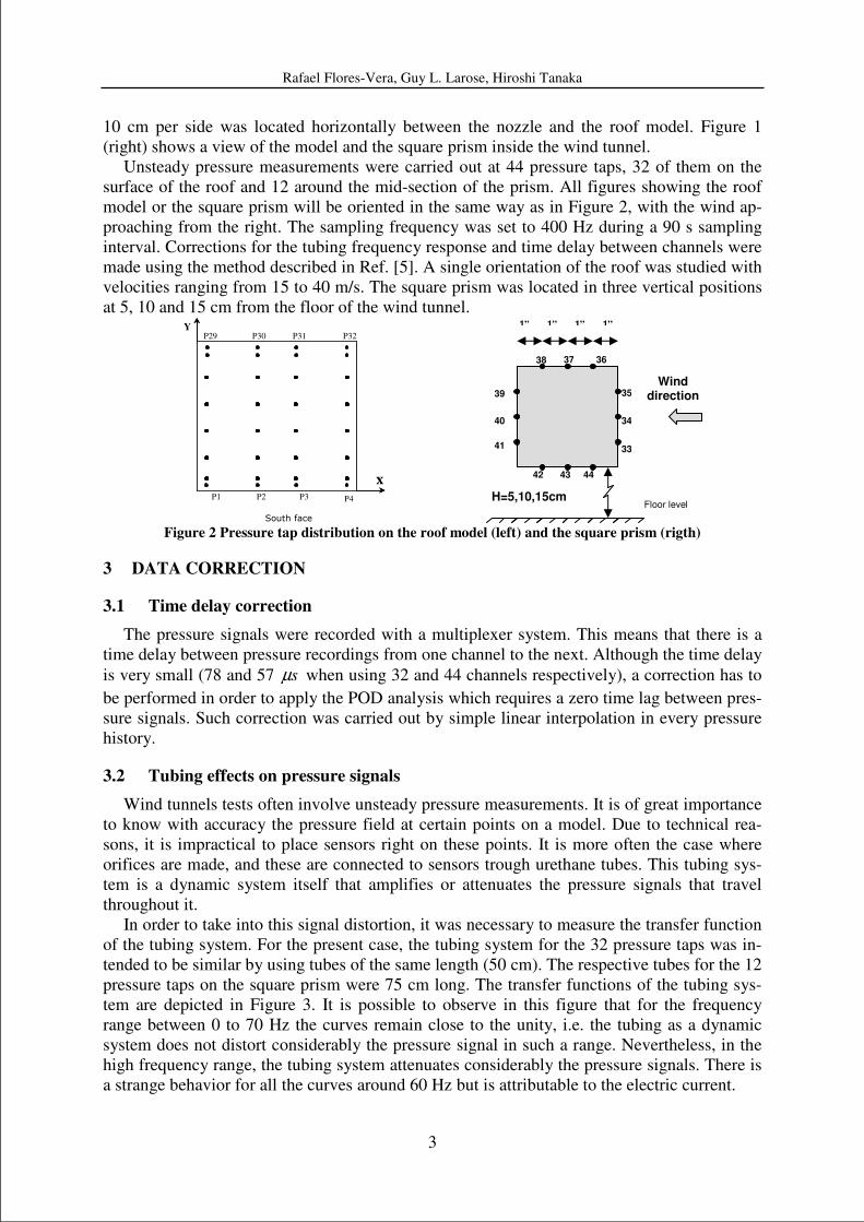
10 cm per side was located horizontally between the nozzle and the roof model. Figure 1

(right) shows a view of the model and the square prism inside the wind tunnel.

Unsteady pressure measurements were carried out at 44 pressure taps, 32 of them on the

surface of the roof and 12 around the mid-section of the prism. All figures showing the roof

model or the square prism will be oriented in the same way as in Figure 2, with the wind ap-

proaching from the right. The sampling frequency was set to 400 Hz during a 90 s sampling

interval. Corrections for the tubing frequency response and time delay between channels were

made using the method described in Ref. [5]. A single orientation of the roof was studied with

velocities ranging from 15 to 40 m/s. The square prism was located in three vertical positions

at 5, 10 and 15 cm from the floor of the wind tunnel.

Figure 2 Pressure tap distribution on the roof model (left) and the square prism (rigth)

3 DATA CORRECTION

3.1 Time delay correction

The pressure signals were recorded with a multiplexer system. This means that there is a

time delay between pressure recordings from one channel to the next. Although the time delay

is very small (78 and 57 sµ when using 32 and 44 channels respectively), a correction has to

be performed in order to apply the POD analysis which requires a zero time lag between pres-

sure signals. Such correction was carried out by simple linear interpolation in every pressure

history.

3.2 Tubing effects on pressure signals

Wind tunnels tests often involve unsteady pressure measurements. It is of great importance

to know with accuracy the pressure field at certain points on a model. Due to technical rea-

sons, it is impractical to place sensors right on these points. It is more often the case where

orifices are made, and these are connected to sensors trough urethane tubes. This tubing sys-

tem is a dynamic system itself that amplifies or attenuates the pressure signals that travel

throughout it.

In order to take into this signal distortion, it was necessary to measure the transfer function

of the tubing system. For the present case, the tubing system for the 32 pressure taps was in-

tended to be similar by using tubes of the same length (50 cm). The respective tubes for the 12

pressure taps on the square prism were 75 cm long. The transfer functions of the tubing sys-

tem are depicted in Figure 3. It is possible to observe in this figure that for the frequency

range between 0 to 70 Hz the curves remain close to the unity, i.e. the tubing as a dynamic

system does not distort considerably the pressure signal in such a range. Nevertheless, in the

high frequency range, the tubing system attenuates considerably the pressure signals. There is

a strange behavior for all the curves around 60 Hz but is attributable to the electric current.

Wind direction

44 43 42

41

40

39

38 37 36

35

34

33

1” 1” 1” 1”

H=5,10,15cm Floor level

X

South face

Y

X

P1 P2 P3 P4

P29 P32 P30 P31


4

Figure 3 Transfer function for all tubes. Channels 1 to 32 (left) and channels 33 to 44 (right)

From the paragraph above, it is expected that the power spectral densities (PSD) from un-

corrected data have lower values in the high frequency range when compared to those PSD of

corrected data. Figure 4 and Figure 5 show that this is true indeed.

Figure 4 Power Spectral Densities for corrected (dot line) and uncorrected (continuous line) data. Roof immersed

in a smooth flow, U=35 m/s

Figure 5 Power Spectral Densities for corrected (dot line) and uncorrected (continuous line) data. Roof immersed

in a vortex trail, U=40m/s

Data standardization (or normalization) is a common practice in experimental work. This

allow to compare the results of similar experiments that were obtained in different scales con-

ditions, either temporal or physical. This mean, for example, that it is possible to compare in-


5

formation of wind pressure measurements obtained in a building with those measurements

obtained in a model inside a wind tunnel.

The power spectral densities may also follow a normalization process, for both the hori-

zontal and vertical axes. The horizontal axis (frequency axis) is multiplied by a factor L/U,

where L is a characteristic length and U is the wind speed. The vertical axis (spectral ampli-

tude axis) is multiplied by a factor 2/ σf , where f is the frequency and 2σ is the variance of

the process.

3.3 Comparison of results between corrected and non corrected data

Since a correction is to be performed, it is interesting to note the impact of the correction

over different parameters and the final results obtained by using the POD.

The first observation is that data correction has no effect on the mean values of pressure

coefficients.

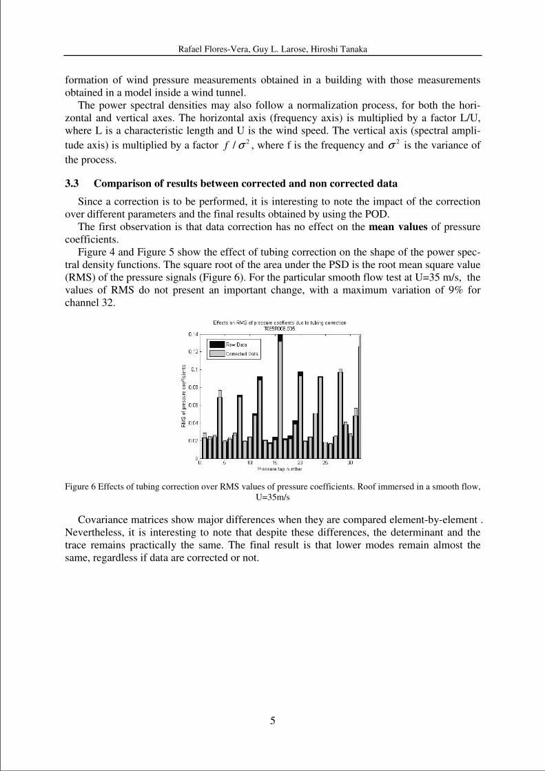
Figure 4 and Figure 5 show the effect of tubing correction on the shape of the power spec-

tral density functions. The square root of the area under the PSD is the root mean square value

(RMS) of the pressure signals (Figure 6). For the particular smooth flow test at U=35 m/s, the

values of RMS do not present an important change, with a maximum variation of 9% for

channel 32.

Figure 6 Effects of tubing correction over RMS values of pressure coefficients. Roof immersed in a smooth flow,

U=35m/s

Covariance matrices show major differences when they are compared element-by-element .

Nevertheless, it is interesting to note that despite these differences, the determinant and the

trace remains practically the same. The final result is that lower modes remain almost the

same, regardless if data are corrected or not.


6

Figure 7 First POD mode for uncorrected (left) and corrected data (right). Roof immersed in a vortex trail,

U=35m/s

The fact that tubing do not have an important influence neither on the statistical parameters

of pressure signals nor the POD results, can be attributed to the characteristics of the transfer

functions of the tubing system. All transfer functions show a value close to the unity from 0 to

70 Hz and it is precisely this range where it is contained most of the energy of the pressure

signals, as can be seen in the PSD functions. This coincidence should not give the wrong im-

pression that tubing correction is unnecessary. Shall the tubes be longer or the wind load con-

tain higher frequencies, the tubing correction would play a more important role.

For the rest of the work, all results will be presented based on the corrected data.

4 ROOF MODEL IMMERSED IN SMOOTH FLOW

The mean pressure coefficient surfaces obtained during this study were found to be similar

in magnitude and shape to those reported in Ref. [3] for flat rectangular roofs. As it is com-

monly observed for bluff body shapes, higher suction values occur near the leading edge,

Figure 8 (left) in the separation bubble.

Figure 8 Iso-contour of mean pressure coefficients (left) and root mean square of pressure coefficients (right).

Roof model immersed in a smooth flow.

The root mean square value (RMS) of the pressure coefficients is an indicator of the level

of unsteadiness in the flow field thus turbulence level, Figure 8 (right). There is a very impor-

tant difference between the RMS values reported here and those reported in Ref. [3], the for-

mer are much lower than the latter. It is apparent that the levels of turbulence of the oncoming

flow should be mainly responsible for this difference but the RMS values remained un-


7

changed even in the case of sub-urban flow. Other factors could be attributed to the curved

shape of the hanging roof which promote reattachment and to the models’ surface roughness.

Since the turbulence levels obtained for the hanging roof are small, it is assumed that the

characteristics of the turbulence observed is mainly local, i.e., the eddies created by the lead-

ing edge are small and/or remain stationary and/or do not travel coherently along the roof.

Consequently the POD is unable to detect a dominant mode, as can be seen in Figure 9 which

shows the energy distribution per mode. The figure shows a comparison with the results re-

ported in Ref. [3].

Figure 9 Cumulative energy distribution per POD mode. Hanging roof (clear), flat roof (dark).

The inexistence of dominant POD modes for the hanging roof contrasts notoriously with

the results obtained for the case of a flat roof, Ref. [3]. In the latter case, the first mode ac-

counts for 95% of the total energy, while the present study shows an energy content of only

20% for the first mode. Furthermore, the shape of the POD modes does not resemble to any of

those reported in the cited paper. Figure 10 shows the first mode.

Figure 10 First POD mode and its normalized spectral density. Roof immersed in a smooth flow.

5 ROOF MODEL IMMERSED IN THE VORTEX TRAIL OF A SQUARE PRISM

The presence of the square prism created mean-velocity and turbulence profiles like those

shown in Figure 11. A schematic representation of the location of the square prism and the

roof model are included in the figure. It is possible to observe a dramatic reduction of wind

speed behind the square prism. This reduction implies velocity gradients which originate a


8

highly turbulent wake, characterized by vortex shedding. An extensive review of vortex shed-

ding from bluff bodies can be found in Refs. [6] and [7].

Figure 11 Left figure: velocity profiles for two cases: smooth flow (dashed line), wind past a square prism (con-

tinuous line). Right figure: Turbulence profile for wind past a square cylinder

Although the POD analysis is carried out for pressure measurements with zero time lag for

all 44 pressure taps, it is convenient to discuss separately some results obtained for the square

prism and for the roof model.

The experiments were performed for three different vertical positions H of the square

prism. It was observed that the proximity of the prism to the floor has an effect on the forma-

tion of vortices, their traveling and the way they impinge the roof located downstream. It is

believed that the proximity of the floor tends to destroy the vortices shed from the bottom face

and/or probably create another structures that affect the vortices shed from the upper face.

Probably more important is the fact that a lower position of the bottom face with respect to the

leading edge of the roof prevent a natural vortex rolling over the roof surface. Actually, the

vortices shed from the bottom face of the prism are stopped by the front wall of the roof

model.

Since the highest position of the prism (H=15cm) provides the best vortex rolling over the

roof surface and also diminishes the floor interaction, such configuration is the most conven-

ient to simplify the study. All the following results were obtained from experiments with the

square prism located at H=15cm from the floor.

5.1 POD analysis for the square prism

The POD reveals flow structures around the square prism. The analysis is based on the un-

steady pressure measurements obtained from 12 pressure taps arranged around the mid span

of the prism -with 3 taps per side.

The mean pressure coefficients (Cp’s) are plotted on Figure 12. These values are practi-

cally the same for wind speeds ranging from 15 m/s to 35 m/s (96,000<Re<224,000) but there

is a 50% of increment in the absolute value recorded in channels 36 to 44 for wind speed of

40 m/s.


9

Figure 12 Mean pressure values for the square prism. U=15-35m/s (left) and U=40 m/s (right)

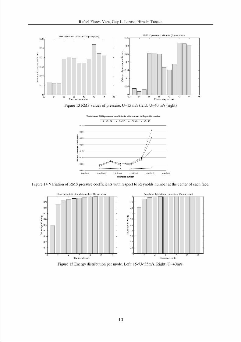
The RMS values of pressure coefficients for the lowest and highest wind speed (15 and 40

m/s) are shown in Figure 13. One may expect a smooth transition between these two graphs,

implying that gradual changes in wind speed will produce gradual changes in turbulence

(measured by RMS). Nevertheless, this was not true. Figure 14 shows the variation of RMS as

a function of Re. It is possible to observe that RMS values remain almost constant for

15m/s<U<35m/s, and so the respective eigenvalues and eigenvectors. However, for U=40m/s

there is a sudden increment in RMS.

The sudden changes in mean and RMS values of pressure coefficients for wind speed

U=40 m/s suggest that a critical speed was reached. This behavior could be attributed to the

lock-in phenomena, which appears when vortex shedding frequency matches the natural fre-

quency of the vortex generator, Ref. [8]. Although the natural frequency for the square prism

was not measured, its numerical estimation is close to 50 Hz. The Strouhal number for square

prisms is estimated between 0.12 and 0.14, Ref. [9]. By using St=0.13, U=40 m/s and L=0.10

m, the vortex shedding frequency is 52 Hz. This close match of frequencies show that the

lock-in phenomena took place at U=40 m/s.

The lock-in phenomena not only increased the RMS values but it actually had a greater ef-

fect on the off-diagonal elements of the covariance matrix of pressure coefficients. This non-

proportional changes in co-variances led to different eigenvalues and eigenvectors. The major

differences are the energy distribution per mode (Figure 15) and the shape of the PSD func-

tion of the second mode (Figure 17 and Figure 18 ).

It is important to mention the strong similarities of the present results with those obtained

in the literature. First of all, the energy distribution (eigenvalues) shown on the right plot of

Figure 15 is completely congruent with that reported in Ref. [1]. Similarly to Refs. [1] and [2],

the first POD mode and its spectral density function clearly show the action of vortex shed-

ding for all wind speeds. The second POD mode and its spectral density function for

15m/s<U<35m/s (Figure 17) also resembles the results obtained in the two references. Such

mode has a similar shape of the mean pressure distribution and it could be regarded as a time-

varying mean pressure.

The differences between the present results and those reported in Refs. [1] and [2] are at-

tributable to different test conditions, being the Re, oncoming flow turbulence and the prism

position inside the wind tunnel the most significant.


10

Figure 13 RMS values of pressure. U=15 m/s (left). U=40 m/s (right)

Variation of RMS pressure coefficients with respect to Reynolds number

0.00

0.05

0.10

0.15

0.20

0.25

0.30

0.35

5.00E+04 1.00E+05 1.50E+05 2.00E+05 2.50E+05 3.00E+05

Reynolds number

RM

S o

f p

ress

ure

co

eff

icie

nts

Ch 34 Ch 37 Ch 40 Ch 43

Figure 14 Variation of RMS pressure coefficients with respect to Reynolds number at the center of each face.

Figure 15 Energy distribution per mode. Left: 15<U<35m/s. Right: U=40m/s.


11

Figure 16 First POD mode in square prism. Similar for all wind speed range.

Figure 17 Second POD mode in square prism. Similar for wind speed range 15<U<35m/s.

Figure 18 Second POD mode in square prism. Wind speed U=40m/s.


12

5.2 POD analysis for the roof model in the vortex trail of the square prism

Since the roof model is immersed in the vortex trail of the square prism, the following re-

sults have to be analyzed in parallel with those reported in the previous section. Particularly, it

is observed again that all results remain practically constant in the wind speed range of 15-35

m/s but there are some noticeable differences when the wind speed reach 40 m/s.

The mean pressure coefficients (Cp’s) are plotted on Figure 19. The Cp’s on the roof re-

main constant for wind speeds between 15 m/s and 35 m/s (left plot). There is a slight varia-

tion on the pressure coefficients obtained for wind speed U=40m/s (right plot).

Figure 19 Mean pressure coefficients for the hanging roof. Left: 15<U<35m/s. Right: U=40m/s.

The RMS values are shown in Figure 20. These values remain practically constant for

15<U<35 m/s (left plot). There is a noticeable change of RMS distribution when the wind

speed reaches 40 m/s (right plot), although the magnitude of the RMS values remain in a

similar range in both plots. The differences in both plots do not seem to be enough reason to

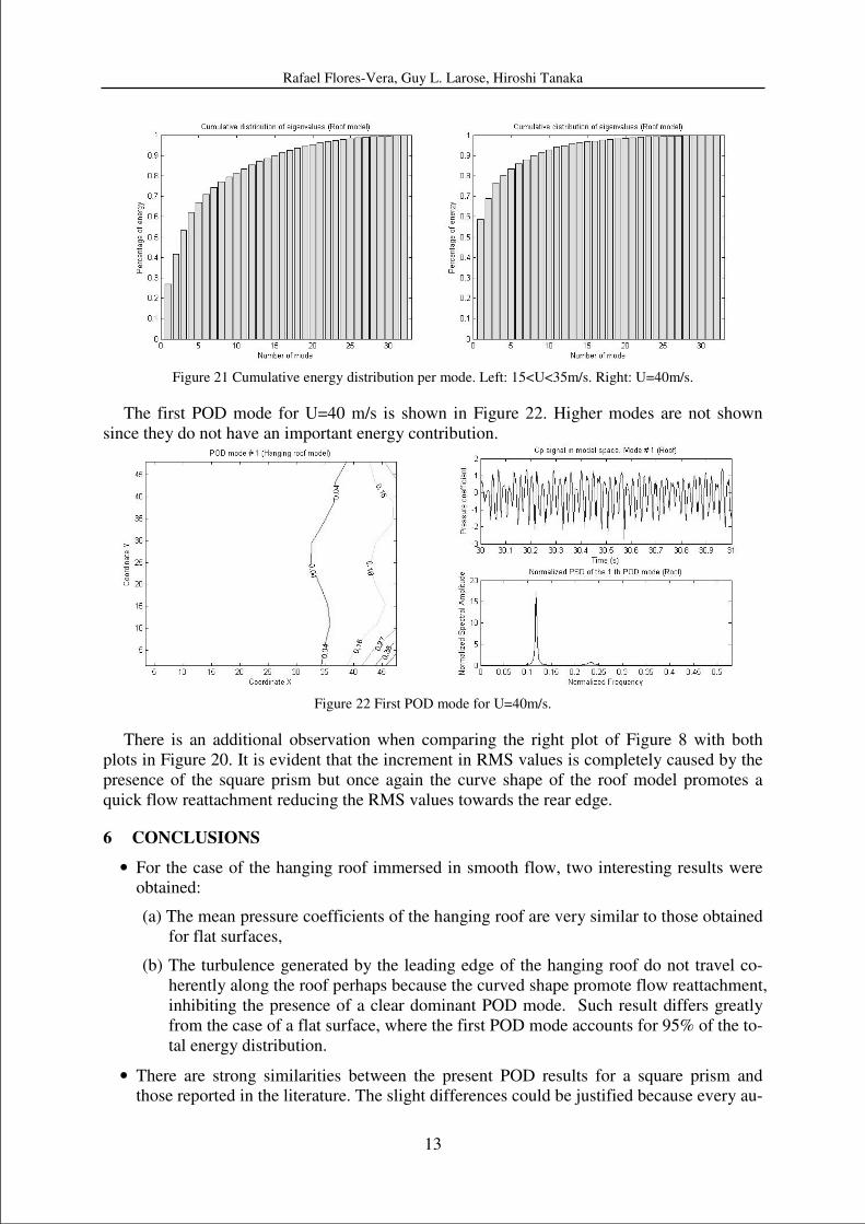
have a dramatic change in their energy distribution, which are shown in Figure 21. Similarly

to the previous section, the reason was found in non-proportional changes in the covariance

matrix elements caused by the lock-in phenomena discussed above.

The differences in covariance matrices with and without the lock-in phenomena have a

drastic effect on their respective energy distribution (eigenvalues) and also in the POD mode

shapes (eigenvectors). As can be seen in the left plot of Figure 21, there is no clear dominant

mode for wind speeds between 15 m/s and 35 m/s. While the right plot of the figure shows an

important increment in the contribution of the first POD mode.

Figure 20 RMS values of pressure for the roof model. Left: 15<U<35m/s. Right: U=40m/s.


13

Figure 21 Cumulative energy distribution per mode. Left: 15<U<35m/s. Right: U=40m/s.

The first POD mode for U=40 m/s is shown in Figure 22. Higher modes are not shown

since they do not have an important energy contribution.

Figure 22 First POD mode for U=40m/s.

There is an additional observation when comparing the right plot of Figure 8 with both

plots in Figure 20. It is evident that the increment in RMS values is completely caused by the

presence of the square prism but once again the curve shape of the roof model promotes a

quick flow reattachment reducing the RMS values towards the rear edge.

6 CONCLUSIONS

• For the case of the hanging roof immersed in smooth flow, two interesting results were

obtained:

(a) The mean pressure coefficients of the hanging roof are very similar to those obtained

for flat surfaces,

(b) The turbulence generated by the leading edge of the hanging roof do not travel co-

herently along the roof perhaps because the curved shape promote flow reattachment,

inhibiting the presence of a clear dominant POD mode. Such result differs greatly

from the case of a flat surface, where the first POD mode accounts for 95% of the to-

tal energy distribution.

• There are strong similarities between the present POD results for a square prism and

those reported in the literature. The slight differences could be justified because every au-


14

thor performed the experiments in different test conditions. In all cases, without excep-

tion, the first POD mode and its power spectral function clearly show that vortex shed-

ding is by far the dominant mode in flow past a square prism.

• The mean and co-variances of pressure coefficients did not change notoriously in the

wind speed range of 15-35 m/s, whereas an appreciable change for those statistics pa-

rameters took place when the wind speed increased to 40 m/s due to the lock-in phe-

nomenon.

• It was found that two tests with similar variances may lead to very different energy dis-

tributions. The reason for this was found in important changes in the co-variances, i.e. the

off-diagonal elements of the covariance matrix.

• Despite the vortices shed from the square prism are highly energetic at the source, they

have a reduced energy contribution when they impinge the roof model. It is believed that

the curved shape of the roof is the main responsible for such reduction.

ACKNOWLEDGEMENTS

The first author acknowledges the financial support from the Consejo Nacional de Ciencia

y Tecnología of Mexico (CONACYT) to carry out his Ph. D. studies in Canada.

REFERENCES

[1] N. Consentino, A. Benedetti. Use of Orthogonal Decomposition Tools in Analyzing

Wind Effect on Structures. Structural Engineering International, 15, 264-270, 2005

[2] H. Kikuchi, Y. Tamura, H. Ueda, K. Hibi. Dynamic Wind Pressures acting on a tall

building model –proper orthogonal decomposition. Journal of Wind Engineering and

Industrial Aerodynamics, 69-71, 631-646, 1997.

[3] B. Bienkiewicz, Y. Tamura, H.J. Ham, H. Ueda, H. Hibi. Proper orthogonal decomposi-

tion and reconstruction of multichannel roof pressure. Journal of Wind Engineering and

Industrial Aerodynamics, 54-55, 369-381, 1995.

[4] Y. Tamura, H. Ueda, H. Kikuchi, K. Hibi, S. Suganuma, B. Bienkiewicz. Proper or-

thogonal decomposition study of approach wind-building pressure correlation. Journal

of Wind Engineering and Industrial Aerodynamics, 72, 421-431, 1997.

[5] G.L. Larose, A. D’Auteuil. On the Reynolds number sensitivity of the aerodynamics of

bluff bodies with sharp edges. Journal of Wind Engineering and Industrial Aerodynam-

ics, in press, 2007.

[6] P.W. Bearman. Vortex shedding from oscillating bluff bodies. Annual Review Fluid

Mechanics, 16, 195-222, 1984.

[7] E. Berger, R. Wille. Periodic flow phenomena. Annual Review Fluid Mechanics, 313-

340, 1972

[8] E. Simiu, R.H. Scanlan. Wind Effects on Structures. John Wiley & Sons, Inc. Third Edi-

tion, p. 217, 1996.

[9] Da-hai Yu, A. Kareem. Numerical simulation of flow around rectangular prism. Journal

of Wind Engineering and Industrial Aerodynamics, 67-68, 195-208, 1997.

Date post:	15-Apr-2018
Category:	Documents
Upload:	votu
View:	216 times
Download:	1 times

THE USE OF THE PROPER ORTHOGONAL …bbaa6.mecc.polimi.it/uploads/validati/nb09.pdfTHE USE OF THE...

Documents