The Use of the Wavelet Transform to Extract Additional Information

6

The Use of the Wavelet Transform to Extract Additional Information on

Surface Quality from Optical Profilometers

Richard L. Lemaster North Carolina State University

USA

1. Introduction

This chapter investigates the use of advanced signal processing techniques especially wavelet transforms to extract additional information from a two dimensional surface profile. The wavelet transform is able to aid the user in quickly assessing, visually, if the surface profile has a periodic or non-periodic component as well as if the profile signal is stationary or non-stationary. In addition, thresholds could be set at different frequencies of interest to automatically determine for the user if a periodic signal is present and if its magnitude is acceptable or not. The basis of this chapter is a doctoral dissertation by Lemaster (2004). A laser based, non-contact profilometer was used for all the surface profiles presented in this chapter though contact profilometers could also benefit from this type of analysis. The original work was conducted for wood and wood-based composites; however the signal processing techniques discussed in this chapter are applicable to all types of surfaces. In fact, an industry that would also like to determine if a surface profile is stationary or not or has periodic components is the road surface industry. They routinely use laser based optical profilometers very similar to the type used in this study except for the optics used to obtain the desired range and sensitivity. They are interested in detecting and quantifying pot holes, ruts, and washboard which are very similar to the surface characteristics of interest to the wood industry but on a different scale.

Traditional time domain analysis that is commonly used in the analysis of surface quality does not adequately show if a periodicity exits on the surface. While frequency domain analysis can reveal if the surface has a periodicity component it cannot adequately determine if the periodicity continues across the entire surface (stationary) or if it only extends across a portion of the surface (non-stationary). This information is of importance if the user wants to extend the capability of traditional surface quality analysis and not only quantify surface irregularities but classify them to both type and source.

2. Background

2.1 Surface texture

Surface texture, a three-dimensional measurement, has been described as the topography, roughness, or irregularity of the interface between a substance and its surroundings,

www.intechopen.com

Advances in Wavelet Theory and Their Applications in Engineering, Physics and Technology 100

generally air (Stumbo, 1963). Surface roughness and surface topography are properties of engineering materials that are important to functional performance and can be used as a measure of product quality and process performance. Surface texture can be caused by the nature of the material itself, a manufacturing process applied to the material, or a combination of both. The processing characteristics that affect the surface texture include: inaccuracy in the machine tool, deformation under cutting force, tool or workpiece vibration, geometry of the cutting action, material tearing during chip formation, and heat treatment effects. Wood characteristics that can affect surface texture include: wood species, density, moisture content, and cutting direction. In most instances, however, surface finish has not been fully exploited in the areas of process monitoring, quality and performance prediction. Today, new measurement techniques and signal processing methods make it feasible to take a new look at the ways available for measuring and evaluating surface texture.

The degree of roughness of a surface often affects the way the material itself is used. In general, surface irregularities can cause misalignment and part malfunctions, excessive loading over small areas, friction and lubrication problems, general finish and reflectivity problems, as well as catastrophic failures. Although surface quality for wood products has been a key issue since woodworking first began, the level of precision required does not approach that found in the metal working industry. This has been due, in part, to wood's inherent dimensional instabilities. The other main reason was that many common uses for wood did not require exceptional surface finishes as compared to many metal applications. The monitoring of surface irregularities in wood is, however, important to assure proper fit of machined parts for gluing, acceptable surface finish for furniture, and as a methodology to monitor the accuracy of the manufacturing process. The last reason has become even more important in recent years due to the increased cost of raw materials, the increased production costs, and the higher production speeds available. Any deviation in expected product quality can quickly cause significant economic losses. There has also been a trend toward tighter tolerances for many forest products industries. An example of this would be the lamination of wood or wood-based products with plastic films or ultra-thin veneers. Even the slightest irregularity in the surface will show through the top laminate.

Usually, wood machining processes are heavily influenced by workpiece surface quality considerations. Tool sharpness requirements as well as machine feed and speed decisions are often based on workpiece surface quality. Research in surface measurement technology was aimed at identifying and quantifying defects associated with a variety of machining processes. Surface waviness is often introduced by the machining process or by the vibration of the tool or workpiece, whereas surface roughness is often introduced by the detachment of material from the workpiece. Of particular interest in this research was the use of frequency domain analysis to separate the random from the periodic components of the surface. The optical profilometer surface measurement system discussed in this chapter has been found to be effective for identifying surface defects including surface waviness, torn grain, fuzzy grain, and abrasive (sanding) grit marks.

Though beyond the scope of this chapter, methods of assessment have ranged from entirely subjective methods (simply feeling the wood surface) to modern day computerized three-dimensional (3D scans) assessments of the surface. The very nature of wood has made the

www.intechopen.com

The Use of the Wavelet Transform to Extract Additional Information on Surface Quality from Optical Profilometers 101

quantitative assessment of surface quality difficult. Wood materials exhibit a wide range of defects due to biological as well as machining-related causes. In some cases there is no clear distinction between biological causes of poor surface quality as opposed to machining related causes.

Monitoring the surface quality of a workpiece surface is a good indicator of the state of the machining process regardless of the workpiece material. It is common practice in wood product industries for lumber graders to check the quality of the surface visually, for composite panel manufacturers to use crayons to check for undesirable sanding marks, for planer operators to “feel” the depth and spacing of planer knife marks, and for saw operators to visually check the severity of saw marks. While these procedures are often used to attempt to determine if a process has varied with time, they are very inconsistent from day to day and do not permit the quantification of the defects. Monitoring the surface quality of a machining process is becoming increasingly important as the machining speed, the cost of raw material, and labor, all continue to increase. Any undetected changes in the quality of machining process can cause a significant impact on the economics of the process.

Workpiece quality evaluation during the actual wood machining process (on–line surface evaluation) has been done using cameras, lasers, x-ray, and various combinations of these technologies. These systems are able to provide a relatively rapid scan of the wood material, usually while the sample is moving slowly (or temporarily stopped on a conveyor) prior to or after being sorted or machined. Such systems are in common use in industry and are aimed primarily at detecting biological defects such as rot, discoloration, knots, etc. These types of systems have also been used to detect simple geometry problems, such as gross dimensional variations, etc.

The work that this chapter is based on consisted of using a laser based position sensing device (PSD) to obtain a 2 dimensional surface profile of the surface. The signal processing techniques that are discussed is an attempt to extract more information as to the type and cause of the surface irregularity than simple measuring the magnitude of the irregularity as is normally done based on the U.S. (ASME B461-2009) and international (ISO 4287/1) standards. The utility of simple frequency analysis is demonstrated below, for several idealized (simulated) examples of surface quality issues relevant to wood machining.

As mentioned above, all examples of surfaces analyzed in this chapter were from wood or wood based products. It is beyond the scope of this chapter to go into detail about wood structure. If interested, the reader is referred to “Understanding Wood” by Hoadley, 2000. The surface texture that is generated when machining wood is very complex and has many factors that can contribute to the variations of the surface quality. Surface defects can be either biological or machining based defects. The fact that wood is an anisotropic and hygroscopic material can cause the surfaces generated by a machining process to vary greatly.

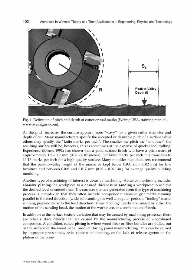
Peripheral milling or planing (moulding) may be defined as the removal of wood in the form of single chips by intermittent engagement of the workpiece with knives carried on the periphery of a rotating cutterhead (Koch, 1955). The resulting surface on the workpiece of a peripheral milling operation consists of individual knife traces generated by successive engagements of each knife or cutting edge (Figure 1). In addition to the height of the ridges or scallops (t), the distance between successive ridges or pitch (Sz) is also an import feature of surface roughness.

www.intechopen.com


Fig. 1. Definition of pitch and depth of cutter or tool marks (Weinig USA, training manual, www.weinigusa.com).

As the pitch increases the surface appears more “wavy” for a given cutter diameter and depth of cut. Many manufacturers specify the accepted or desirable pitch of a surface while others may specify the “knife marks per inch”. The smaller the pitch the “smoother” the resulting surface will be, however, this is sometimes at the expense of quicker tool dulling. Experience (Effner, 1992) has shown that a good surface finish will have a pitch mark of approximately 1.5 – 1.7 mm (0.06 – 0.07 inches). For knife marks per inch this translates to 15-17 marks per inch for a high quality surface. Many moulder manufacturers recommend

that the peak-to-valley height of the marks be kept below 0.005 mm (0.02 in) for fine

furniture and between 0.005 and 0.017 mm (0.02 – 0.07 in.) for average quality building moulding.

Another type of machining of interest is abrasive machining. Abrasive machining includes abrasive planing the workpiece to a desired thickness or sanding a workpiece to achieve the desired level of smoothness. The surfaces that are generated from this type of machining process is complex in that they often include non-periodic abrasive grit marks running parallel to the feed direction (wide belt sanding) as well as regular periodic “tooling” marks running perpendicular to the feed direction. These “tooling” marks are caused by either the motion of the sanding head, the motion of the workpiece, or a combination of both.

In addition to the surface texture variation that may be caused by machining processes there are other surface defects that are caused by the manufacturing process of wood-based composites. A condition, called pitting is where wood fiber or fiber bundles are pulled out of the surface of the wood panel product during panel manufacturing. This can be caused by improper press times, resin content or blending, or the lack of release agents on the platens of the press.

www.intechopen.com


2.2 Conventional surface quality measurement and analysis techniques

Vast amounts of work have been conducted in attempts to develop techniques to measure and evaluate surface texture in materials. These techniques generally fall into two distinct groups. The first is the hardware or method to measure surface texture data. The second is the analysis procedure to evaluate the surface texture. Numerous methods have been developed and researched for both the measurement and evaluation techniques. Measurement techniques normally fall into two distinct categories: contact and non-contact methods. It is beyond the scope of this chapter to discuss the surface measurement techniques that have been investigated in the past. The reader is referred to Lemaster (2004) for an overview of the various works on this topic. A general review of the optical techniques (and surface roughness techniques in general) is provided in several comprehensive reference works (Thomas, 1999; Whitehouse, 2011; Whitehouse, 1994; Thomas and King, 1977; and Riegel, 1993). The work conducted by the author on optical profilometry of wood and wood-based products can also be found in the literature (Lemaster, 2010, Lemaster, 2004; Lemaster 1997a, 1997b; Lemaster and Beall, 1996; Lemaster and DeVries, 1992; Lemaster and Dornfeld, 1983; Jouaneh, Lemaster, and Dornfeld, 1987; and DeVries and Lemaster, 1992).

The heart of any surface quality assessment system is the detector. The optical method used for the detector in this research is a variation of the reflectance method, whereby the positional change of the reflected laser light into the detector is correlated to changes in the test surface height. In this method, a laser spot is projected on the workpiece surface and the reflected light is focused on the surface of a lateral-effect photodiode. The change of the position of the reflected laser spot on the surface of the detector, a’ is correlated to the vertical height change of the workpiece, a. By moving a workpiece beneath the detector and recording the change in the position of the laser spot, a two-dimensional surface profile is obtained that is very similar to that obtained by the traditional stylus system (Figure 2). The resulting surface profile can then be analyzed according to traditional U.S. (ASME B461-2009) and international standards (ISO 4287/1). This method is non-contact and capable of detection at high speed, and since it measures position changes of the reflected light and not spot intensity, it is relatively insensitive to color changes of the workpiece.

Fig. 2. Schematic of optical profilometer

Detector

a’

a

Wood Surface

Laser

www.intechopen.com


2.2.1 Time domain characterization

Most surface quality analysis including three-dimensional analysis has been traditionally

based upon the surface tracing or surface profile. Most analysis of the surface profile

generated by the stylus system has been evaluated using time domain parameters such as

height deviations and asperity spacing or wavelength. Whitehouse (1982) gives a brief

history of the development of surface quality evaluation techniques and the confusion that

has developed due to new developments in measurement technology, lack of coordinated

efforts between countries, changes in manufacturing processes resulting in different surface

textures for a given part, and economic considerations affecting instrumentation

development. King and Spedding (1983) discussed three categories of approaches that have

been used to characterize a surface:

Characterization by process specification (sawing, milling, etc.)

Characterization according to function (intended use of workpiece)

Statistical characterization of the surface profile (magnitude of surface irregularities,

etc.)

The figure below (figure 3) shows a common example of time domain measurements. The

measurements include a measure of the average roughness, Rq (second moment, root mean

square), a measure of "extremes" Rtm, a measure of whether the surface defects are above or

below the average surface, a measure of skewness, Rsk (third moment), and a measure of the

shape of the surface defects, Rku kurtosis (4th moment).

Fig. 3. Definitions of surface descriptors

2.2.2 Frequency domain characterization

Although wood surface description is the main subject here, the potential advantages of

frequency analysis has been investigated for metal surface measurement as well as road

Distance (inch or mm)

0.0 0.5 1.0 1.5 2.0 2.5

Su

rfa

ce

He

igh

t Z

(in

or m

)

-40

-20

0

20

40Evaluation Length (L)

Rmax

Sample Length (l)

Z1

Z2

Zi

Mean or Reference Line

Rq = [Z1

2 + Z2

2 + Z3

2 + Zi

2 + ... ZN

2/N]

0.5

Rtm = mean value of the Rmax of

five consecutive sample lengths (l)

Rsk = (1/Rq

3)(1/N)Zi

3

Rku = (1/Rq

4)(1/N)Zi

4

www.intechopen.com


surface measurement. The use of standard surface descriptors based on time domain

analysis is sufficient for some applications; however it does not provide information as to

the periodicity of the surface characteristics or the nature or cause of the defects. Frequency

is most often expressed as cycles per second known as Hertz (Hz). However, frequency can

also be expressed spatially such as cycles per unit length (cycles per inch).

As stated by Brock (1983), in the field of signal processing and analysis as applied to sound

and vibration problems, the transformation of the signal from the time domain to the

frequency domain is very common due to the ease with which the signal can be analyzed

and characterized. Although this approach is not common in the field of surface quality

analysis, the same benefits can be realized. The main advantage of frequency analysis is that

it can reveal the dominant frequency components contained in the transducer signal. Ber

and Braun (1968) showed that the frequency spectra resulting from the measurements on

surfaces obtained by turning, grinding, and lapping are dissimilar. Raja and Radhakrishnan

(1979) separated the roughness from the waviness component on a surface by using fast

Fourier transform techniques. Staufert (1979) also used frequency domain analysis to

separate periodic components from random components in the surface. In the literature an

industry that has tended to use the power spectrum for surface quality analysis is that of

road surface evaluation. In an article by Bruscella, Rouillard, and Sek (1999) a laser based

optical profilometer was used to obtain a surface profile of the road. Both the time and

frequency domains were analyzed.

Work by Lemaster (1997b) has addressed the use of the frequency spectrum of the surface

profile to detect "periodicity" within a surface profile. This approach is suitable because a

surface profile is often composed of both random and periodic components. Under ideal

cutter conditions, the tool produces evenly spaced cutter marks which occur periodically. In

cases where the tool is not concentric, out of balance, or the workpiece is not properly held,

the marks are unevenly spaced and vary in depth. More random defects often result from

the detachment of material from the workpiece. The utility of simple frequency analysis is

demonstrated, for several idealized (simulated) examples of surface quality issues relevant

to wood machining is discussed below.

Much work has been conducted on using wavelets in filtering or de-composing the surface profile. The category of interest here is the use of wavelets to separate these surface components. Much of the work discussing wavelets as applied to surface roughness are based on analyzing the gray scales of an image of the surface which is beyond the scope of this chapter and will not be discussed here but the reader is referred to Fricout et. al. (2002) for one discussion of this approach. Other works discussing wavelets and surface texture consists of multi-resolution decomposition of the surfaces including separating the error of form, waviness, roughness, and localized defects. Work by Khawaja (2011) demonstrated the insensitivity of the shape of the wavelet in its ability to decompose the components of a surface trace and obtain a standard roughness descriptor. While these works are very important in the complete understanding of surface texture analysis, it was not the main thrust of the topic in this chapter. In fact, the work by Lemaster (2004) found that this use of wavelets did indeed provide a means of removing the form of the surface texture that, in many cases, yielded superior filtering than the traditional phase correct Gaussian filter.

www.intechopen.com


2.2.3 Shortcomings of simple time and frequency analysis

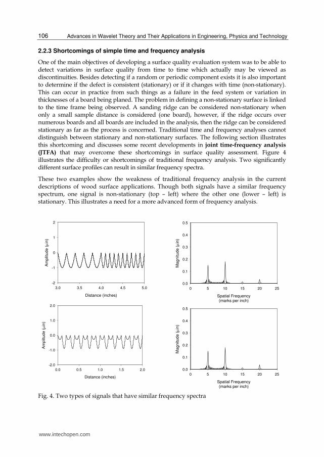
One of the main objectives of developing a surface quality evaluation system was to be able to detect variations in surface quality from time to time which actually may be viewed as discontinuities. Besides detecting if a random or periodic component exists it is also important to determine if the defect is consistent (stationary) or if it changes with time (non-stationary). This can occur in practice from such things as a failure in the feed system or variation in thicknesses of a board being planed. The problem in defining a non-stationary surface is linked to the time frame being observed. A sanding ridge can be considered non-stationary when only a small sample distance is considered (one board), however, if the ridge occurs over numerous boards and all boards are included in the analysis, then the ridge can be considered stationary as far as the process is concerned. Traditional time and frequency analyses cannot distinguish between stationary and non-stationary surfaces. The following section illustrates this shortcoming and discusses some recent developments in joint time-frequency analysis (JTFA) that may overcome these shortcomings in surface quality assessment. Figure 4 illustrates the difficulty or shortcomings of traditional frequency analysis. Two significantly different surface profiles can result in similar frequency spectra.

These two examples show the weakness of traditional frequency analysis in the current descriptions of wood surface applications. Though both signals have a similar frequency spectrum, one signal is non-stationary (top – left) where the other one (lower – left) is stationary. This illustrates a need for a more advanced form of frequency analysis.

Fig. 4. Two types of signals that have similar frequency spectra

Distance (inches)

3.0 3.5 4.0 4.5 5.0

Am

plit

ud

e ( in

)

-2

-1

0

1

2

Distance (inches)

0.0 0.5 1.0 1.5 2.0

Am

plit

ud

e (in

)

-2.0

-1.0

0.0

1.0

2.0

Spatial Frequency(marks per inch)

0 5 10 15 20 25

Magn

itude ( in

)

0.0

0.1

0.2

0.3

0.4

0.5


0 5 10 15 20 25

Magn

itude ( in

)

0.0

0.1

0.2

0.3

0.4

0.5

www.intechopen.com


3. Basic joint time / frequency analysis

3.1 The Short Time Fourier Transform (STFT)

The FT is very versatile, but is inadequate when one is interested in the “local” (in time or space) frequency content of the signal. A transform method that can analyze non-stationary signals where the frequency information changes with time is required for this type of analysis.

An obvious method, following on from the FT, is to analyze the time (space) signal over 0-T seconds in a train of shorter intervals such as 0-T/4, T/4-T/2, T/2-3T/4, 3T/4-T, known as windows (Figure 5).

Fig. 5. Short Time Fourier Transform (STFT) with moving non-overlapping rectangular windows.

The individual windows, being only of length T/4 in this case, mean that the lowest frequency fL will be only one-quarter of the full 0-T window value. This method, first described by Gabor (1956), is known as the Short Time Fourier Transform (STFT), (see Goswani and Chan (1999) and Qian (2002) for a full discussion). Today, the individual transforms are usually performed using the FFT algorithm where the window shape can be varied; i.e. rectangular, Hanning, cosine taper, etc.

Note in an STFT, as in the FT, the size of the window is fixed but the frequency of the sinusoids that are compared to the signal varies as does the number of oscillations. A small window is unable to detect low frequencies which are too large for the window. If too large a window is used then information about a brief change will be lost. This implies prior knowledge of the signal’s characteristics and will become an important criterion for choosing the analysis method. An additional advantage of the non-overlapping STFT is that perfect reconstruction of the original signal g(t) is still possible.

A more recent, but slower, method known as the adaptive Gabor spectrogram was developed by Qian and Chen (1994) where the time and frequency resolutions are defined by one parameter. Unlike the classical Gabor expansion, where the time and frequency resolutions are fixed, the time and frequency resolutions of the adaptive Gabor expansion can be adjusted optimally. This method while, it would be acceptable for “off-line” surface measurements was not investigated further in this research because of the slower computational times and the desire to have an efficient method that could be used on-line in a manufacturing environment.

0 T/4 T/2 3T/4 T

t

www.intechopen.com


An improvement to the STFT time-frequency analysis method is to overlap the windows. Figure 6 demonstrates the sliding window principle.

Fig. 6. Example of Sliding Short Time Fourier Transform

With digitized data, the limit to the time resolution is to move the window one sample at a time to yield up to N windows. There is a clear improvement in time resolution and with present day computer speeds so fast, there is little slowdown in the computation.

3.2 The Wavelet Transform

The JTFA methods such as the STFT and Wigner-Ville have been criticized for their failure to resolve both time and frequency simultaneously. This led to a search for other functions, besides sine and cosine waves to overcome this problem. These local basis functions, which have been studied in incredible mathematical detail in recent times, are typically used for analyzing non-stationary signals and are known as wavelets. Each wavelet is located at a different position along the time (space) axis which decreases to zero on either side of the center position, (see Figure 7) such that the average value (area under the wavelet) is zero. Wavelets are not necessarily of fixed frequency and can be either compressed or dilated in time, which results in a change of scale (see Figure 8). Much like the FT and STFT, multiplication of the signal g(t) by the wavelet shapes as basis functions yields a set of coefficients which describe the correlation between the signal and the wavelet. In particular, depending on the wavelet shape, discontinuities in the signal can be easily detected.

Fig. 7. Morlet mother wavelet function (Hubbard, 1998)

www.intechopen.com


Fig. 8. Example of wavelet compression (top) and dilation (bottom)

Further examination of figure 8 shows that, unlike the STFT (where the size of the windows are fixed, filled with oscillations of the sine and cosine waves of different frequencies) the reverse is now true in that the number of oscillations is fixed (the mother wavelet shape) but the window width or scale is varied. If the window is stretched, the wavelet frequency is decreased to analyze low frequencies (long times). When the window is compressed, analysis of high frequencies (short times) is possible. Hubbard (1998) called this technique a “mathematical microscope”. This initial wavelet shape may be viewed as the mother wavelet from which all the other wavelets (in this function class or shape) can be derived.

The concept is thus more complicated than the FT in that not only does the multiplying function contain multiple frequencies, but changes its center frequencies as it changes its scale. To overcome the time and resolution uncertainty effect it will be seen that many window (wavelet) widths or resolutions can be written into one algorithm. Although the original idea of the wavelets can be traced back to the Haar transform first introduced in 1910 (a German paper published in the Mathematical Annals, Volume 69), wavelets did not become popular until the early 1980’s when researchers in geophysics, theoretical physics, and mathematics developed the mathematical foundation (see Qian, 2002). Hubbard (1998) stated that tracing the history of wavelets was almost a job for an archaeologist. Meyer (1989) stated that he had found at least 15 distinct roots of the wavelet theory. Since then considerable work has been conducted by mathematicians and to a lesser degree by engineers. Uses of wavelets were discovered; in particular Mallet (1989) and Meyer (1989) found a close relationship between wavelets and the structure of multi-resolution analysis. Mallat stated that a multi-resolution transform of the signal is equivalent to a set of filters of constant percentage bandwidth in the frequency domain. Work by Mallet and Meyer led to a simple way of calculating the mother wavelet as well as a connection between continuous wavelets and digital filter banks. Following this work, Daubechies (1990) further developed a systematic technique of generating finite duration wavelets using sets of discrete difference equations to calculate the wavelet shape. They are designated D4, D20, etc. denoting the number of wavelet describing coefficients, Daubechies (1990).

It is not the intent of this chapter to cover the mathematical details of wavelets. The reader can find a comprehensive treatment of wavelet analysis and descriptions in Burrus (1998), Daubechies (1990), Mallat (2009), Newland (1997), and Strang and Nguyen (1996). For a less intense mathematical treatise of wavelets, the reader is referred to Hubbard (1998).

www.intechopen.com


3.2.1 Description of wavelets

While both STFT (and other JTFA techniques) and wavelets can be used for time-frequency analysis, they each have a distinct set of advantages and disadvantages. The STFT is suited for narrow instantaneous frequency bandwidths (such as chirps), while the wavelet (time-scale) transforms are best suited for signals that have instantaneous peaks or discontinuities (image description, sound generated by engine knocks, etc.) (Qian, 2002).

There are two major categories of wavelet transforms; continuous and discrete (Gaberson, 2002). According to Gaberson, the continuous wavelet transform (CWT) is easier to describe. The CWT is a “short wavy” function that is stretched or compressed and placed at many positions along the signal to be analyzed. The wavelet is then term-by-term multiplied with the signal, each product yielding a wavelet coefficient value. Just as the STFT with its non-overlapping time windows historically came before the (continuous) sliding STFT so have applications of the discrete wavelet transform (DWT) historically come before the CWT. In the DWT there will be a finite number of wavelet comparisons whereas in the CWT there could be an infinite number. Since this chapter is part of a book on applications of wavelets and is companioned with a book on the theory of wavelets the background of wavelets will not be discussed in detail here.

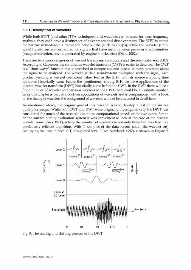
As mentioned above, the original goal of this research was to develop a fast online surface quality technique. While both CWT and DWT were originally investigated only the DWT was considered for much of the research due to the computational speeds of the two types. For an online surface quality evaluation system it was convenient to look at the case of the discrete wavelet transform (DWT), where the number of wavelets is not only finite but also lead to a particularly efficient algorithm. With N samples of the data record taken, the wavelet (t) occupying the time interval 0-T, designated level 0 (see Newland, 1997), is shown in Figure 9.

Fig. 9. The scaling and shifting process of the DWT

www.intechopen.com


Next the wavelet is compressed time-wise into two similar shapes of the same amplitude by a factor of one-half to form level 1, then again by another factor of one-half to form 4 wavelets at level 2, etc. Level -1 is the DC level of the signal. These wavelets are compared to the signal by multiplication generating the coefficients W(s,). Plotting the square of these coefficients yields a 3-dimensional time-scale or time-frequency plot similar to the STFT.

As a reminder, each multiplication of a wavelet with a part of the signal is a correlation or comparison of the signal with the wavelet and is called the wavelet transform coefficient W(s,). Note each wavelet waveform contains the same number of oscillations unlike the STFT described earlier. Following Newland (1997), with N samples of the data with N = 2n there will be n+1 levels of wavelet analysis (including the -1 level). There are n sets of wavelet multiplications. If N = 128 = 27 there will be 1, 2, 4, 8, 16, 32, and 64 wavelet compressions describing the shifts from level 0 through level 7. Note that the total number of multiplications is 127 which is of order (N). Following Hubbard (1998), if each wavelet is described or supported by c samples, the number of multiplications is cN. Thus the DWT is of the same order of computational efficiency as the FFT (where Nlog2N multiplications are required) for typical values of n.

The alternative filter bank approach (Strang and Nguyen, 1996) looks at data signals conceptually in the frequency domain. Approaching the method via the DWT, each wavelet behaves as a band-pass filter in the frequency domain (see Figure 10).

Fig. 10. Bandwidth of data windows for STFT (top) and DWT (bottom)

A third technique proposed by Newland (1993) is based on the fast Fourier transform (FFT) using an exact octave-band filter shape defined in the frequency domain (e.g. from

frequency 1 to 2). Fourier coefficients are processed in octave-bands to generate wavelet coefficients by an orthogonal transformation which is implemented by the FFT. Unlike wavelets generated by discrete dilation equations whose shapes cannot be expressed in functional form, harmonic wavelets have the simple structure:

Bandwidth of STFT window

Bandwidth of CWT window

www.intechopen.com


( 4 ) 2 )( ) / 2j t j tt e e j t (1)

This function is concentrated locally around t = 0, and is orthogonal to its own unit translations and octave dilations. Its frequency spectrum is confined exactly to an octave-band so that it is compact in the frequency domain instead of the time domain, see Figure 11, which shows a comparison of the Newland harmonic wavelet with the Daubechies D20 wavelet in the frequency domain (Newland, 1993). The Newland harmonic wavelet, being complex, can incorporate phase like some other wavelets but its amplitude decreases to zero at a slower rate of 1/t than some other wavelets. The Newland harmonic wavelet has been found to be particularly suitable for vibration and acoustic analysis because its harmonic structure is similar to naturally occurring signal structures and, therefore, they correlate well with experimental signals.

D20 Harmonic

Fig. 11. Comparison of the Daubechies - D20 (a) and Newland harmonic wavelets (b) in the time domain as well as the frequency domain (c)

Generally there is no exact simple relationship between the scale (s) and frequency (f), except to say that scale is approximately inversely proportional to the frequency so that high frequencies refer to low scales and vice versa. An advantage of the Newland harmonic wavelet is that he is able to use an accurate frequency axis in place of scale and the scale axis may be exactly written as the inverse frequency.

3.2.2 Wavelet selection

A challenge exists in choosing a wavelet best suited for analyzing wood surfaces. Due to the desire to detect small localized defects, a high sample density is needed (i.e. in the range of

www.intechopen.com


8192 samples per inch). Obtaining this level of sampling, on-line and in real-time makes the speed of the analysis process critical. As mentioned before, the literature is full of different wavelet functions but very little advice is presented in the literature on choosing the best wavelet for the task. The advice normally is to choose a wavelet that is “similarly” shaped to the signal to be analyzed and then to try several wavelets. Hubbard (1998) devotes an entire chapter to discussing which wavelet should be used. There are definite differences of opinions on the procedure to follow. One is to use the commonly used wavelets such as the Mexican Hat and Morlet. The other extreme is to develop a new wavelet for a particular purpose. The question, as discussed in Hubbard, then arises as to what are the properties that are desired for the new wavelet. While the desire may be in trying to get fine resolution for both time and frequency domain, this is impossible and violates the uncertainty principle.

As mentioned in a previous section, periodic knife marks on a surface are a primary surface defect of interest in wood machining. Usually the higher the frequency of the knife marks, the lower the amplitude and the less objectionable the marks. From a series of field tests conducted as part of this research it was found that objectionable knife marks on moulder and planers as well as sanding “chatter” marks on wide belt sanders often occur in the range of 5 marks per inch.

3.2.3 Comparison of STFT and harmonic wavelet

In the research presented by Lemaster (2004) the various DWT and CWT were compared to the STFT. In addition, direct comparisons between the Harmonic and Daubachies D20 DWT techniques were also conducted. As mentioned previously, the CWT techniques did not provide enough increase in resolution to justify the added computational intensity. Also, a benefit of the Harmonic DWT was that it provided direct frequency information instead of scaling information which is only indirectly proportional to the frequency. So for the remainder of this discussion, a comparison was done between the more established Short Time Fourier Transform (STFT) and the Newland Harmonic DWT.

A series of simulated signals (waves) were generated to compare the ability of the two techniques to detect simulated surface defects including changing frequency and a localized defect (scratch or gouge on wood). The resulting plots were shown in units of length of scan and spatial frequency (marks per inch) to illustrate the plots in terms of spatial frequency for the actual surface scans. The plots consisted of 8192 data points over a 1 inch length of simulated scan. The STFT and DWT plots that were conducted on a reduced data set (every 16th data point for faster calculation speed) missed small defects such as the scratch. As discussed above, for larger defects such as the presence of a periodic component, the reduced data set still yielded a sufficient sampling frequency for the frequency and joint time/frequency analysis while maintaining the high sampling density required for time domain analysis. The first series of comparison was between two sine waves (5 Hz and 20 Hz). These frequencies were chosen because they approximate a single knife and a four knife finish on a typical moulder or planer operation. Two versions of the sine waves can exist, the first is when the two frequencies are superimposed on each other as when there are two sources of machine vibration and the second condition is when the two frequencies are appended to each other as when the feed rate has changed due to an alteration or slippage of the feed system (Figure 12).

www.intechopen.com


Fig. 12. Time domain signal of two superimposed sine waves (left) and two appended sine waves (5 Hz and 20 Hz)

Figure 13 (left) shows the time-frequency plot of the STFT of the two appended sine waves.

From this figure it can be seen that a ridge is detected at 5 Hz extending from 0 to 1.0 second

and a second ridge is detected at 20 Hz extending from 1.0 to 2.0 seconds. The edges of the

ridges are sloped and not sharp. Similarly in Figure 13 (right), which shows the time-

frequency plot of the appended sine waves for the HWT, the two ridges are detected at 5

and 20 Hz and extending only half way across the time axis as they should. The ridge at 5

Hz, however, is not as well defined as the ridge at 20 Hz.

Fig. 13. STFT plot (left) of two appended sine waves (5 Hz and 20 Hz)(used every 16th point of 16384 point data file, 256 point window moved at 2 point intervals and Harmonic wavelet (right)(used every 16th point of 16384 point data file)

From these two figures, it appears that both the STFT and the harmonic wavelet can easily

detect the two appended sine waves and provide information regarding where in the time

domain the frequency of the sine waves change. The harmonic wavelet appeared to

attenuate the lower frequency on the appended sine waves. The STFT attenuated the edges

of the ridges at both frequencies.

Time (sec)

0.0 0.5 1.0 1.5 2.0

Am

plit

ud

e

-3

-2

-1

0

1

2

3

Time (sec)

0.0 0.5 1.0 1.5 2.0

Am

plit

ude

-3

-2

-1

0

1

2

3

www.intechopen.com


The next set of simulated surface scans was for a localized defect such as a dent or scratch in the surface while still having knife marks. Since the lower frequencies of knife marks have proven to be more difficult to detect, a surface scan of 5 marks per inch with a small scratch in the surface was simulated. This surface profile is shown in Figure 14. This signal had a 5 Hz sine wave with a peak-to-peak amplitude of 2.0 and a scratch that had an amplitude of 1.5. Figure 15 show the STFT and harmonic wavelet plots respectively. Both the STFT and the harmonic wavelet detected the scratch in the surface. The STFT had to be adjusted so that the length of the analysis window and the amount to advance the window each time was much smaller than previous analyses. This means that a prior knowledge of the type of defect expected is required in order to use the STFT method on-line. Though this configuration of the STFT could detect the scratch, it resulted in a loss of resolution in detecting the 5 Hz sine wave. The harmonic wavelet could detect the scratch with no adjustments to the analysis. Additional tests for both the STFT and the harmonic wavelet showed that the scratch had to be larger than the peak height of the sine wave to be detected. Neither the STFT nor the harmonic wavelet could detect the scratch of a simulated surface scan that had a scratch amplitude of 1.0 with the 5 Hz sine wave having a 2.0 peak to peak amplitude. This means that a scratch would have to be at least of the same magnitude of the knife marks in order to be detected. The Newland HWT has the advantage in that frequency is accurately plotted rather than scale and its use was chosen for the signal analysis of the remainder of this research.

Fig. 14. Simulated surface profile of 5 Hz sine wave (5 marks per inch) with “scratch”

Fig. 15. STFT (left) and HWT (right) of 5 Hz sine wave with “scratch”

Scan Length

0.0 0.5 1.0 1.5 2.0

Am

plit

ud

-2.0

-1.5

-1.0

-0.5

0.0

0.5

1.0

1.5

www.intechopen.com


4. Results of surface scans

This section will show the results of using the HWT for various surfaces. In review, the surface quality assessment system is being designed to assist wood product manufacturers in monitoring their machining operations and alert them if the operation or the product quality changes during the machining process. To that end, the system must be able to scan the surface, analysis the data and make a decision on the state of the operation in an acceptable time frame. Information in the frequency domain can be limited to below 50 marks per inch since very high spatial frequencies are not of importance to the manufacturer. However, higher frequencies still must be included in order to detect the localized defects in the frequency domain.

4.1 Sanding ridge caused by loss of abrasive

This defect is caused by a portion of the abrasive in an abrasive machining operation

separating from the backing of the abrasive belt. This is often caused by the belt striking a

foreign object in the surface of the workpiece. The result is a ridge which forms on the

surface of the workpiece. Figure 16 shows a photograph of a cabinet door with two

sanding ridges on it. This results in a defect that is localized in one location of the surface

of the workpiece; but is also considered stationary in that it occurs along the entire length

of the surface as well as subsequent workpiece surfaces. This defect is very similar to a

machining defect that is caused by a nick in a blade on a moulder, planer, or router. The

surface profile for the sanding ridge shows the ridges very clearly (see Figure 17, left). The

frequency plot (Figure 17, right) shows very little information or periodicity. The

harmonic wavelet plot (see Figure 18) also shows no periodicity but does show the two

sanding ridges and the location (in time) where they occur. The wavelet coefficients are

negligible over most of the plot; with the two peaks caused by the two sanding ridges

clearly shown at both ends of the scan. The advantage of the harmonic wavelet transform

is that it shows both time and frequency information together in a single plot. The HWT

clearly shows the two peaks and when they occurred as well as the fact that no significant

periodicity exists on the surface.

Fig. 16. Photograph of specimen with sanding ridges caused by loss of abrasive

www.intechopen.com



0 20 40 60 80 100

Ma

gn

itu

de

(in

)

0

200

400

600

800

1000

Distance (inches)

0.0 0.5 1.0 1.5 2.0 2.5 3.0

Am

plit

ud

e ( in

)

-10000

-5000

0

5000

10000

Fig. 17. Profile (left) and frequency spectrum (right) of specimen with sanding ridges caused by loss of abrasive

Fig. 18. Harmonic wavelet transform of specimen with sanding ridges

4.2 Surface with varying frequency of knife marks

This section shows a situation in which the knife marks occurring on the surface change in

frequency along the length of the surface. This type of surface defect could be due to

slippage occurring in the feed works of the machining operation or a slowing of the

cutterhead rpm due to motor overload. This type of defect may be both non-stationary

(among different workpieces) as well as non-stationary within a workpiece. Figure 19 shows

a photograph of this type of surface characteristic. The surface profile (Figure 20, left) shows

the varying wavelengths as well as the varying amplitudes on the surface of the workpiece.

The frequency spectrum (Figure 20, right) shows the difference in the amplitude of the two

frequencies as well as the difference in the spatial frequencies. The harmonic wavelet plot

(Figure 21) shows the predominant frequency extending across the majority of the surface

scan but changing in amplitude but also with varying frequencies present like a chirp. This

plot also shows how the frequency changes along the length of the surface.

www.intechopen.com


Fig. 19. Photograph of surface with varying frequency of knife marks

Fig. 20. Profile (left) and HWT (right) of surface with varying frequency of knife marks

Fig. 21. Harmonic wavelet transform of surface with varying frequency of knife marks


0 5 10 15 20

Ma

gnitu

de

( in

)

0

2000

4000

6000

8000

10000

Scan Length (inch)

0.0 0.5 1.0 1.5 2.0 2.5 3.0 3.5

Am

plit

ude ( in

)

-10000

-5000

0

5000

10000

www.intechopen.com


5. Decision making scheme

The final step in developing an on-line surface quality monitoring system was the decision making scheme to determine if an unacceptable condition is present. As mentioned before, one of the objectives was to be able to determine from the data if a surface defect is periodic versus non-periodic and stationary versus non-stationary in nature. This aids the operator in determining the cause of the surface defect and what remedial action to take.

As discussed previously, the time-frequency plots provide information on the magnitude of the surface defect as well as determining if the defect is stationary or non-stationary. There are two approaches to interpreting the time-frequency plots. The first approach is to treat the time-frequency plot as an image and use standard image analysis techniques to determine the magnitude and shape of any “peaks” or “ridges” in the plot. A small diameter “blob” of the color representing a high mean-square value would represent a severe localized defect; whereas a long smear or ridge of the same color would represent a severe periodic condition. Since only the lower periodic frequencies (i.e. less than 50 knife marks per inch) are of interest for machined wood surfaces, the higher frequencies can be combined together for analysis of both non-periodic and localized defects. The second approach is to simply look at the data array representing the time-frequency plot of the harmonic wavelet analysis. For the examples shown, a surface profile generated by 16384 data points resulted in a time-frequency plot array of 15 x 4096 with the 15 columns representing the 15 frequency bandwidths (bins) of the HWT. This second approach was the one used in this research.

The first step in classifying a defect is to determine whether the surface defect is periodic, non-periodic, localized, or a combination of two or more of these categories. One approach is to view the periodic, non-periodic, and localized defects on an x, y, z plot. Since three parameters are required to describe a point in three space, the values of the three surface defect categories would indicate where in space the current specimen falls. A perfectly smooth surface would be at the origin of the plot. As a surface develops greater surface defects (regardless of the type or category of defect), the value on the plot moves further away from the origin. If the value for a periodic defect is higher than the value for the non-periodic defect then the surface in question is more periodic than non-periodic.

There are several methods of determining where along the three-space defect category axes a surface defect falls. One way is to conduct traditional time and frequency analysis and determine the best surface descriptor for the type of defect of interest in each category. The three surface descriptors would then be plotted in three-space with the magnitude of the defect (surface descriptor) being normalized before being plotted.

From the time-frequency plots it can be seen the HWT can differentiate between extreme conditions and can provide the user with comprehensive information about the type of surface that has been scanned. The difference between the periodic and non-periodic situations can be determined by setting a threshold and then counting the number of data excursions above the threshold to indicate that the signal has a periodic component. A single threshold crossing could indicate a scratch or other localized defect. Since only periodic components below 50 marks per inch are typically of interest, only lower frequency bins would need to be monitored for periodic components. The frequency bins representing

www.intechopen.com


periodicities (knife marks) greater than 50 marks per inch can be grouped together and used to monitor overall roughness.

By monitoring the amplitudes of the bins of interest (less than 50 marks per inch) and setting an amplitude threshold then a frequency bin that would have, for example, 25 percent of the amplitude values over the amplitude threshold would be considered slightly periodic AND slightly stationary. If 50 percent of the data points in a frequency bin exceeded the threshold value then the signal would be considered slightly periodic and moderately stationary. If the amplitudes exceeded a secondary threshold value then the surface would be considered moderately periodic. An example of the action of the controller is if 5% of data points, at a given frequency, exceed the threshold then the defect was considered a peak (representing a localized defect). If 25% of the points at a given frequency exceed the threshold value then the defect is considered a slight ridge. If 50% of the points exceed the threshold then the defect is considered a medium ridge. This continues for a long ridge and a complete ridge.

A problem can arise when the surface descriptors get close to the threshold but do not exceed it. An example would be when only slightly less than 25 percent of the amplitude values exceeded the threshold value, which, based on traditional techniques, would be considered non-stationary. The interpretation of the 3-dimensional plots of the results from the time-frequency analysis, while being somewhat easy by a human, is difficult when attempting to have a computer automatically make decisions on the state of the manufacturing process. The approach that was evaluated here was to use fuzzy logic to decide where in three-space the specimen or workpiece of interest belonged. A detailed discussion of using fuzzy logic for surface quality evaluation can be found in Lemaster (2004). Two applications of fuzzy logic were evaluated. The first was to use the standard surface descriptors to determine if a primary surface defect present on a specimen was periodic or not and then the second was to use the results of the HWT to determine if the periodic surface defect was stationary or non-stationary.

6. Conclusion

The overall goal of the research was to be able to detect an unacceptable surface produced

during a machining operation and then attempt to provide additional information to the

machine operator regarding the type of defect, the degree of the defect, and the possible

source of the defect. In manufacturing, a defect that extends above the surface such as a

ridge along the surface is usually much easier to deal with (repair) than a defect that extends

below the surface such as a gouge or fiber tear-out. It is also desirable to determine if a

surface defect is periodic, random-like, or localized in nature. In addition, it is also desirable

to determine if the defect is stationary or non-stationary as referenced to the surface of one

specimen (it has been shown that a wood machining operation in which tool wear occurs is

technically a non-stationary process when considering multiple specimens).

As discussed previously an example of a periodic surface are the knife marks from a planer or moulder. An example of a random-like surface would be fuzzy grain. An example of a localized surface defect would be a dent or a ridge caused by a chip in the cutting tool. The difference between a stationary or a non-stationary defect is that a stationary defect would extend along the entire length of the workpiece whereas a non-stationary defect would occur only along a portion of the workpiece.

www.intechopen.com


This research compared various JTFA techniques including the STFT as well as numerous discrete wavelet transforms (DWT) on their ability to detect where in time a periodicity exists on the surface of a wood or wood-based composite product. This research concluded that the Harmonic DWT or HWT worked best from an efficiency in computational time as well as its ability to detect both low frequency periodicity as well as localized defects. From the time-frequency plots it can be seen the HWT can differentiate between extreme conditions and can provide the user with comprehensive information about the type of surface that has been scanned. The difference between the periodic and non-periodic situations can be determined by setting a threshold and counting the number of data excursions above the threshold to indicate whether the signal has a periodic component or not. A single threshold crossing could indicate a scratch or other localized defect. Since only periodic components below 50 marks per inch are typically of interest, only lower frequency bins need to be monitored for periodic components. The frequency bins representing periodicities (knife marks) greater than 50 marks per inch can be grouped together and used to monitor overall roughness. A two tier fuzzy logic scheme was devised to determine if the surface profile had a periodicity or was localized and / or if the surface defect was stationary or non-stationary in nature.

Current and future work includes collecting data on the ability of the system to perform in a variety of manufacturing environments and at a variety of manufacturing speeds.

7. Acknowledgements

The author would like to thank Professor Thomas H. Hodgson for his invaluable help in learning and applying the JTFA techniques discussed in this chapter.

This work was funded by a United States Department of Agriculture: Wood Utilization Research Center Grant.

8. References

American Society of Mechanical Engineers, 2009. Surface Texture (Surface Roughness,

Waviness, and Lay). ASME B46.1-2009. ISBN: 9780791832622, ASME New York.

United Engineering Center, 345 East 47th Street, New York, NY 10017.

Ber, A., and S. Braun, 1968. Spectral analysis of surface finish. CIRP Annals, Vol. 16, pp. 53-

59, ISSN: 0007-8506.

Brock, M., 1983. Fourier analysis of surface roughness. Bruel & Kjaer Technical Review,

ISSN: 0007-2621, Marlborough, Mass., No. 3, 48 pages.

Bruscella, B., V. Rouillard, and M. Sek, 1999. Analysis of road surface profiles. Journal of

Transportation Engineering, Vol.125(1):55-59, ISSN: 0733-947X.

Burrus, C. S., 1998. Introduction to Wavelets and Wavelet Transforms – A Primer. Prentice Hall,

ISBN: 0134896009, Upper Saddle River, NJ.

Daubechies, I., 1990. The wavelet transform, time-frequency localization, and signal

analysis, IEEE Trans. Information Theory, pp. 961-1005, ISSN: 0018-9448.

DeVries, W.R. and R.L. Lemaster, 1991. Processing methods and potential applications of

wood surface roughness analysis. Proceedings of the 10th International Wood

Machining Seminar, October 21-23. pp. 276-292.

www.intechopen.com


Effner, J., 2001. How depth of cut affects finish quality. FDM, January: 120-121.

Fricout, G., D. Jeulin, P.-J. Krauth, and T. Jacquot, 2002, Automatic on-line inspection of non-

smooth surface, Wear Vol. 264:416-421, ISSN: 0043-1648.

Gaberson, H. A., 2002. The use of wavelets for analyzing transient machinery vibration.

Sound and Vibration, Vol. 36(9):12-17 ISSN: 1541-0161.

Hoadley, R. B., 2000, Understanding Wood: A Craftman’s Guide to Wood Technology, Taunton

Press, ISBN: 1-56156-358-8 Newton, CT, 280 pages.

Hubbard, B. B., 1998. The World According to Wavelets, second edition, A. K. Peters, LTD.,

ISBN: 1-56881-072-5, Wellesley, Massachusetts. 330 pages.

ISO Standard 4287/1, "Surface Roughness - Terminology - Part 1: Surface and Its

Parameters," 1984.

ISO Standard 4287/2, "Surface Roughness Terminology - Part 2: Measurement of Surface

Roughness Parameters," 1984.

Jouaneh, M.K., R.L. Lemaster, and D.A. Dornfeld, 1987. Measuring workpiece dimensions

using a non-contact laser detector system. International J. of Advanced

Manufacturing Technology, Vol. 2(1):59-74, ISSN: 0268-3768.

Koch, P., 1955. An analysis of the lumber planing process: part I, Forest Products Journal

5:255-264, ISSN: 0015-7473.

Khawaja, Z., G. Guillemot, P.-E.Mazeran, M. El Mansori, and M. Bigerelle, 2011, Wavelet

theory and belt finishing process, influence of wavelet shape on the surface

roughness parameter values, 13th International Conference on Metrology and

Properties of Engineering Surfaces, Journal of Physics: Conference Series 311:

012013, pages 1-5.

Lemaster, R.L. and D.A. Dornfeld, 1982. Measurement of surface quality of sawn and

planed surfaces with a laser. Proceedings of the 7th Wood Machining Seminar,

October 1982, University of California Forest Products Laboratory, Richmond, CA,

pp. 52-70.

Lemaster, R.L. and W.R. DeVries, 1992. Non-contact measurement and signal processing methods

for surface roughness of wood products. Proceedings of the 8th International

Symposium on Nondestructive Testing of Wood, September 23-25, 1991.

Vancouver, WA, pp. 203-218.

Lemaster, R.L., and F.C. Beall, 1996. The use of an optical profilometer to measure surface

roughness in medium density fiberboard. Forest Products Journal, Vol.

46(11/12):73-78, ISSN: 0015-7473.

Lemaster, R.L., 1997. The use of an optical profilometer to monitor product quality in

wood and wood-based products. Proceedings of the National Particleboard

Association Sanding and Sawing Seminar, Charlotte, NC, November 1995,

published by the Forest Products Society, ISBN: 0-935018-51-4, Madison,

Wisconsin, USA, 17 pages.

Lemaster, R.L., 1997. Hardwood machining R&D: surface quality and process monitoring

technologies. Proceedings of the Eastern Hardwood Resource, Technologies, and

Markets Conference. April 21-23, Camp Hill, Pennsylvania. Published by the Forest

Products Society, pp. 109-120.

www.intechopen.com


Lemaster, R.L., 2004. Development of an Optical Profilometer and the Related Advanced Signal

Processing Methods for Monitoring Surface Quality of Wood Machining Applications.

Doctoral dissertation, North Carolina State University, ISBN 9780496147298, 254

pages.

Lemaster, R.L., 2010. The use of frequency and wavelet analysis for monitoring surface quality of

wood machining applications. Scanning, The Journal of Scanning Microscopies:

Special Issue on Diverse Applications of Surface Metrology I, July/August 2010,

Volume 32, Issue 4, Pages 224 - 232, Issue edited by: Christopher A. Brown. ISSN:

1932-8745

Mallat, S., 2009. A Wavelet Tour of Signal Processing, third edition, Academic Press, ISBN:

13-078-0-12-374370-1, Burlington, Maryland, USA.

Mallat, S., 1989. Multifrequency channel decompositions of images and wavelet models.

IEEE Trans. Acousitcs, Speech, Signal Processing, Vol.(37):2091-2110, ISSN: 0096-

3518.

Newland, D. E., 1993. Harmonic wavelet analysis. Proceedings Royal Society London, A

Vol.(43):203-225 ISSN: 0962-8444.

Newland, D. E., 1997. An Introduction to Random Vibrations, Spectral and Wavelet Analysis,

Third Addition, Addison Wesley Longman Limited, ISBN: 0-582-21584-6

Edinburgh, Harlow. 477 pages.

Qian, S., 2002. Introduction to Time-Frequency and Wavelet Transforms, Prentice Hall PTR,

ISBN: 0-13-030360-7, Upper Saddle River, N.J., 280 pages.

Qian, S. and D. Chen, 1996. Joint Time-Frequency Analysis. Prentice Hall, ISBN-13: 978-

0132543842, Upper Saddle River. New Jersey.

Raja, J. and V. Radhakrishnan, 1979. Filtering of surface profiles using fast Fourier

transform. Int. J. Mach. Tool Des. Res. 19:133-141.

Riegel, A., 1993. Quality measurements in surface technologies. International Conference on

Woodworking Technologies, Conference at the Ligna 1993, Hannover, Germany.

April 20-23. pp. 23.1-23.10.

Staufert, G. 1979. Description of roughness profile by separating the random and periodic

components. Wear 57:185-194, ISSN: 0043-1648.

Strang, G. and T. Q. Nguyen, 1996. Wavelet and Filter Banks, Prentice Hall, ISBN-13: 978-

0961408879, Upper Saddle River, NJ, 484 pages.

Stumbo, D., 1963. Surface texture measurement methods. Forest Prod. J. 13(7):299-304, ISSN:

0015-7473.

Thomas, T. R., 1981. Characterization of Surface Roughness. Precision Engineering Vol. 2:97-

104, ISSN: 0141-6359.

Thomas, T.R. and M. King, 1977. Surface topography in engineering - a state of the art review and

bibliography. Cotswold Press LTD, ISBN-13: 978-0900983665.

Thomas, T. R., 1999, Surface Roughness, 2nd Edition, Imperial College Press, London,

England, ISBN: 1-86094-100-1, 278 pages.

Whitehouse, D. J., 1994. Handbook of Surface Metrology, Institute of Physics Publishing,

London, England, ISBN: 0-7503-0039-6, , 988 pages.

www.intechopen.com


Whitehouse, D. J., 2011. Handbook of Surface and Nanometrology, 2nd Edition, CRC Press,

Taylor and Francis Group, Boca Raton, FL, U.S.A, ISBN: 1978-1-4200-8201-2, 976

pages.

www.intechopen.com

Advances in Wavelet Theory and Their Applications inEngineering, Physics and TechnologyEdited by Dr. Dumitru Baleanu

ISBN 978-953-51-0494-0Hard cover, 634 pagesPublisher InTechPublished online 04, April, 2012Published in print edition April, 2012

InTech EuropeUniversity Campus STeP Ri Slavka Krautzeka 83/A 51000 Rijeka, Croatia Phone: +385 (51) 770 447 Fax: +385 (51) 686 166www.intechopen.com

InTech ChinaUnit 405, Office Block, Hotel Equatorial Shanghai No.65, Yan An Road (West), Shanghai, 200040, China

Phone: +86-21-62489820 Fax: +86-21-62489821

The use of the wavelet transform to analyze the behaviour of the complex systems from various fields startedto be widely recognized and applied successfully during the last few decades. In this book some advances inwavelet theory and their applications in engineering, physics and technology are presented. The applicationswere carefully selected and grouped in five main sections - Signal Processing, Electrical Systems, FaultDiagnosis and Monitoring, Image Processing and Applications in Engineering. One of the key features of thisbook is that the wavelet concepts have been described from a point of view that is familiar to researchers fromvarious branches of science and engineering. The content of the book is accessible to a large number ofreaders.

How to referenceIn order to correctly reference this scholarly work, feel free to copy and paste the following:

Richard L. Lemaster (2012). The Use of the Wavelet Transform to Extract Additional Information on SurfaceQuality from Optical Profilometers, Advances in Wavelet Theory and Their Applications in Engineering, Physicsand Technology, Dr. Dumitru Baleanu (Ed.), ISBN: 978-953-51-0494-0, InTech, Available from:http://www.intechopen.com/books/advances-in-wavelet-theory-and-their-applications-in-engineering-physics-and-technology/the-use-of-the-wavelet-transform-to-extract-additional-information-on-surface-quality-from-optical-p

© 2012 The Author(s). Licensee IntechOpen. This is an open access articledistributed under the terms of the Creative Commons Attribution 3.0License, which permits unrestricted use, distribution, and reproduction inany medium, provided the original work is properly cited.

http://creativecommons.org/licenses/by/3.0

Date post:	03-Feb-2022
Category:	Documents
Upload:	others
View:	3 times
Download:	0 times

The Use of the Wavelet Transform to Extract Additional Information

Documents