The utility of expectational data: Firm-level evidence using matched qualitative-quantitative UK surveys * Silvia Lui, James Mitchell and Martin Weale National Institute of Economic and Social Research October 6, 2010 Abstract Qualitative expectational data from business surveys are widely used to con- struct forecasts. But, based typically on evaluation at the macroeconomic level, doubts persist about the utility of these data. This paper evaluates the ability of the underlying firm-level expectations to anticipate subsequent outcomes. Im- portantly this evaluation is not hampered by only having access to qualitative outcome data obtained from subsequent business surveys. Quantitative outcome data are also exploited. This required access to a unique panel dataset which matches firms’ responses from the qualitative business survey with these same firms’ quantitative replies to a different survey carried out by the national statisti- cal office. Nonparametric tests then reveal an apparent paradox. Despite evidence that the qualitative and quantitative outcome data are related, we find that the expectational data offer rational forecasts of the qualitative but not the quantita- tive outcomes. We discuss the role of “discretisation” errors and the loss function in explaining this paradox. * We thank the CBI and the ONS for their help in facilitating this project, with particular thanks to Lai Co (CBI), Rhys Davies (ONS), Robert Gilhooly (ONS), Felix Ritchie (ONS), Eric Scheffel (ONS), Richard Welpton (ONS) and Jonathan Wood (CBI). Thanks to two anonymous referees for helpful comments. We gratefully acknowledge financial support from the ESRC (Award Reference: RES-062- 23-0239) and the Bank of England. This work contains statistical data from ONS which are Crown copy- right and reproduced with the permission of the controller of HMSO and Queen’s Printer for Scotland. The use of the ONS statistical data in this work does not imply the endorsement of the ONS in relation to the interpretation or analysis of the statistical data. This work uses research datasets which may not exactly reproduce National Statistics aggregates. For more details about the CBI’s ITS, please go to http://www.cbi.org.uk/ndbs/content.nsf/802737AED3E3420580256706005390AE/2F172E85D0508CEA80256E20003E95C6. 1
Transcript
The utility of expectational data: Firm-level evidenceusing matched qualitative-quantitative UK surveys∗
Silvia Lui, James Mitchell and Martin WealeNational Institute of Economic and Social Research
October 6, 2010
Abstract
Qualitative expectational data from business surveys are widely used to con-struct forecasts. But, based typically on evaluation at the macroeconomic level,doubts persist about the utility of these data. This paper evaluates the abilityof the underlying firm-level expectations to anticipate subsequent outcomes. Im-portantly this evaluation is not hampered by only having access to qualitativeoutcome data obtained from subsequent business surveys. Quantitative outcomedata are also exploited. This required access to a unique panel dataset whichmatches firms’ responses from the qualitative business survey with these samefirms’ quantitative replies to a different survey carried out by the national statisti-cal office. Nonparametric tests then reveal an apparent paradox. Despite evidencethat the qualitative and quantitative outcome data are related, we find that theexpectational data offer rational forecasts of the qualitative but not the quantita-tive outcomes. We discuss the role of “discretisation” errors and the loss functionin explaining this paradox.
∗We thank the CBI and the ONS for their help in facilitating this project, with particular thanks toLai Co (CBI), Rhys Davies (ONS), Robert Gilhooly (ONS), Felix Ritchie (ONS), Eric Scheffel (ONS),Richard Welpton (ONS) and Jonathan Wood (CBI). Thanks to two anonymous referees for helpfulcomments. We gratefully acknowledge financial support from the ESRC (Award Reference: RES-062-23-0239) and the Bank of England. This work contains statistical data from ONS which are Crown copy-right and reproduced with the permission of the controller of HMSO and Queen’s Printer for Scotland.The use of the ONS statistical data in this work does not imply the endorsement of the ONS in relationto the interpretation or analysis of the statistical data. This work uses research datasets which may notexactly reproduce National Statistics aggregates. For more details about the CBI’s ITS, please go tohttp://www.cbi.org.uk/ndbs/content.nsf/802737AED3E3420580256706005390AE/2F172E85D0508CEA80256E20003E95C6.
1
1 Introduction
Qualitative business surveys are widely seen as an important complement to official
data. These surveys typically ask businesses to provide qualitative categorical answers
to a number of questions including what has happened to their output in the recent past
and what they expect to happen to their output in the near future. Respondents say
whether output has fallen, stayed the same or risen and which of the three they anticipate
over some specified future period. The importance that the European Commission
attaches to such surveys can be seen from the fact that it meets a part of their costs and
publishes their findings monthly. The Bank of England refers to them in its minutes
(Bank of England (2010)) and it is clear that the European Central Bank also regards
them as informative; e.g., see Trichet (2009). As compared to official data they have
two major attractions. First they are more timely. Secondly they provide indicators
of expectations as well as outcomes. Expectational data are used widely by forecasters
on the assumption that they tell them something useful about what will happen to the
economy in the future.
Despite the growing interest in micro data, analysis of such data focuses, almost
universally, on aggregate summaries of the findings. Such summaries typically show
the proportions of the respondents in each of the three categories mentioned above.
Or they are limited to indicating the “balance of opinion”- the difference between the
proportion of those expecting or reporting a rise and those expecting or reporting a
fall. For example, the cross-country expectational business survey data archived by the
European Commission are presented in this latter form. These data are available at
However, a small but growing literature has peered into the ‘black box’ to examine
the underlying firm-level qualitative data. When these data take the form of a panel,
such that it is possible to keep track of the expectations and outcomes as reported by
individual firms, then it is possible to test their utility directly. One can test whether
firms’ expectations are, in any statistical sense, coherent with the outcomes that they
subsequently report. There have been a few applications of such tests. Nerlove (1983)
compared French and German firms’ qualitative expectations with their subsequent qual-
itative reports of what actually happened using 3×3 contingency tables constructed from
their trichotomous ordered responses. Horvath et al. (1992) and Ivaldi (1992) tested ra-
tionality using the (polychoric) correlation matrix between the categorical variables.
There are, in fact, two types of analysis which can profitably be carried out using such
2
micro data. The first is an examination of the answers that businesses give to different
questions in the survey, with the comparison of the qualitative expectations they report
in one survey and the qualitative outturn they report in a subsequent survey being only
one example. The second is a comparison of the answers businesses give in qualitative
surveys with the quantitative data that the same firms provide in (usually distinct)
surveys such as those used in compiling output indices and national accounts. Obviously
for this second type of analysis to be carried out, it is necessary to obtain or generate
matched data sets which contain the answers of a given firm to both types of survey. We
are not aware of business surveys being analysed in this way previously, perhaps because
of the difficulties in obtaining suitable data. There are, however, studies of household
expectations and quantitative and qualitative outcomes. These are facilitated because
the same survey typically collects both types of data. For example Das et al. (1999)
look at the Dutch Socio-Economic Panel.
In this paper we draw on a panel dataset of UK manufacturing firms’ responses to the
Industrial Trends Survey, run by the Confederation of British Industry, and the Monthly
Production Inquiry, run by the Office for National Statistics. This dataset matches firms’
responses from a leading qualitative business survey with these same firms’ quantitative
replies to a different official survey carried out by the national statistical office. We then
test the ability of firm-level expectations to anticipate subsequent outcomes. Extending
previous work, this evaluation exploits both qualitative and quantitative outcome data.
Specifically, we use and develop nonparametric tests for the rationality of the firm-level
qualitative expectational data. Rationality tests remain a useful tool in assessing the
utility of expectational data. This is because under rationality outcomes do not differ
systematically (i.e., regularly or predictably) from what was expected. But for qualita-
tive expectations data implementation of rationality tests requires additional auxiliary
assumptions to be made which are tested jointly with rationality. We therefore follow
Manski (1990) and Das et al. (1999) and, more accurately, refer to the tests as tests of
the “best-case scenario”. In particular, we discuss how the implications of rationality
depend on the firm’s loss function. Under rationality different loss functions result in
different categorical predictions, given the firm’s subjective density forecast. We there-
fore follow Das et al. (1999) and conduct tests when firms report the mode, the median
(more generally the alpha-quantile) or the mean of their subjective density forecast of
future output growth. These tests follow Manski (1990) and identify bounds on the
distribution of realised outcomes conditional on firms’ qualitative expectations under
3
the assumption of rational expectations.
As well as testing the ability of the expectational data to forecast the two distinct
outcome variables, we test what we call the coherence between these qualitative and
quantitative outcome measures. This involves testing whether the two outcome variables
are measuring the same concept of output growth, as implicitly assumed when outcome
data from qualitative business surveys are used to provide a contemporaneous indication
(nowcast) of economic activity. With its access to a unique matched panel dataset this
paper represents, to the best of our knowledge, the first application of these tests to
business surveys of the type routinely used by forecasters.
The next section explores previous uses and tests of expectational data. It motivates
our use of nonparametric tests to judge the utility of these data when collected in qual-
itative business surveys and available at the micro-level. It also explains why we prefer
to speak of the specific rationality tests employed as tests of the “best-case scenario”,
given that auxiliary assumptions need to be made to operationalise the rationality test
with categorical expectations data. Section 3 provides a description of the data that
we use. We then present our notation in Section 4. This is followed in Section 5 by
a detailed discussion of the tests that can be carried out on these expectations data.
Section 6 describes the results of the tests and Section 7 concludes.
2 Background
Expectations are subjectively held beliefs of individuals or firms about uncertain future
outcomes. Most published expectations data are concerned with point expectations,
although recently there has been increased interest in density expectations or forecasts;
e.g., see Hall & Mitchell (2009). Density forecasts provide an estimate of the probabil-
ity distribution of the possible future values of the variable and represent a complete
description of forecast uncertainty. In contrast, point expectations represent just one
feature of this subjective density. As we discuss below, which feature is extracted de-
pends on the forecaster’s loss function. Our focus is on qualitative point expectations,
since business surveys tend to take this form. But importantly, depending on the fore-
caster’s loss function, we evaluate these expectational data relative to both qualitative
and quantitative outcome or realisations data.
4
2.1 Uses of expectational data
Expectational data continue to be used widely as leading indicators by forecasters. For
some recent examples published in the International Journal of Forecasting see Kauppi
et al. (1996), Hansson et al. (2005), Abberger (2007) and Claveria et al. (2007). Ex-
pectational data are also used in conjunction with other variables when forecasting.
Factor models, for example, are a popular tool to produce forecasts from a large set
of indicator variables, only some of which may be expectational variables; see Stock &
Watson (2002) and Forni et al. (2001). The use of expectational data is predicated on the
hope that models that include expectational information deliver more accurate forecasts
than models without expectations. Typically these expectational data are considered in
“aggregate” form, as proportions of the respondents in each of the three categories, con-
sidered above, or as the balance of opinion. An exception is Mitchell et al. (2005) who
considered how to construct indicators of the aggregate of interest from the underlying
qualitative firm-level panel dataset. Their indicator gives more emphasis to firms whose
qualitative answers have a close link to the official data than to those whose expectations
correspond only weakly or not at all.
Expectational data are also used to test different models of expectations formation,
notably rationality (see Section 2.2 below). They are also used to test different economic
theories. For examples, see Nerlove (1983), McIntosh et al. (1989), Horvath et al. (1992),
Carroll et al. (1994), Branch (2004), Easaw & Heravi (2004) and Souleles (2004). As well
as the European Commission’s qualitative business surveys, qualitative expectational
data are also collected for Japan by Tankan and for the US by the Michigan Survey of
Consumer Attitudes and Behavior and The Conference Board.
Quantitative expectations data, typically forecasts from professional economists, are
also available from Consensus Economics (for most countries in the world), Blue Chip
Economic Indicators (principally the US), the Livingstone Survey (US) and the Survey
of Professional Forecasters (US). Having the expectations data in quantitative form is
more informative. But the number of forecasters, N , surveyed is much smaller (typically
N < 100) than in business surveys of the sort we study in this paper, where N is typically
at least ten times bigger.
Nevertheless, doubts persist about the quality and utility of these expectational
data. This is explained, at least in part, by the qualitative nature of data typically
available from business tendency surveys. Other reasons include a priori concerns that
respondents do not mean what they say when subjectively replying to surveys; e.g., see
5
Bertrand & Mullainathan (2001). There are also a posteriori doubts. This is because of
mixed empirical evidence on: (i) whether models with expectations data deliver more
accurate forecasts than models without expectations data and (ii) whether expectations
are formed “rationally”, a term we define below. Pesaran & Weale (2006) provide a
survey of this evidence, with the findings of Claveria et al. (2007) exemplifying the
inconclusive evidence on the utility of expectational data when forecasting. Moreover,
in a recent application Wheeler (2010) found that while recessions in the UK have been
preceded by large deteriorations of expectations, the expectational data have given false
signals in the past.
This paper extends the coverage of empirical work by assessing the utility of these
qualitative expectational data at the firm level not just in terms of their relationship
with firms’ own retrospective but qualitative reports of their output growth but with
these same firms’ quantitative answers.
2.2 Rationality
Tests of the rationality of expectations remain a useful first step in establishing the
utility of expectational data. But the specific rationality test implemented, and the
auxiliary assumptions needed, depend on the nature of the available expectations data.
In particular, the test depends on whether aggregated (macro) data or micro data are
used. It also depends on whether the expectations data are available in quantitative or
qualitative form.
The rational expectation is defined as the “objective” expectation of the outcome
conditional on the set of all information relevant to the determination of the outcome
available at the time the expectation was made. With rationality, outcomes do not differ
systematically (i.e., regularly or predictably) from what was expected. People know
“how the world works” and their (“generalised” - discussed further below) forecasting
errors are unbiased, serially uncorrelated at the single period horizon and orthogonal
to information known at the time the forecast was made; see Patton & Timmermann
(2007a). When coupled with the assumption that people form their point forecasts
under a mean squared error loss function rational point forecasting errors share these
properties. But more generally, as shown by Patton & Timmermann (2007a), it is a
transformation of the forecasting error called the generalised error that possesses these
properties under rationality. This transformation accommodates the fact that rational
forecasters may not be attempting to minimise expected mean squared error loss, but a
6
more general potentially asymmetric loss function.
When the expectation takes the form of a density forecast, rationality requires equal-
ity of this subjectively formed density with the objective probability density function
from which the outcome is drawn. Mitchell & Wallis (2010) review tests for the equality
of these two densities, operational when, as is usual in practice, we do not observe the
objective density itself but a draw from it. But more commonly, as with the case we
discuss below, only a point expectation is available.
2.2.1 Aggregate tests
In the absence of expectations data joint tests of rationality are required, since expecta-
tions are typically inferred from observed aggregate data conditional on a behavioural
model (e.g., see Wallis (1980)). This means any test for rationality also depends on the
choice of behavioural model. But the availability of (point) expectations data facilitates
direct tests of rationality. Most studies have tested rationality assuming mean squared
error loss. This involves testing the unbiasedness and efficiency of the expectations data
(e.g., see Brown & Maital (1981); and Clements & Hendry (1998), pp. 56-59, for a
textbook discussion). But tests under more general, asymmetric loss have also been
developed. They reflect the aforementioned fact that it is the generalised forecasting
error that is conditionally and unconditionally unbiased; see Patton & Timmermann
(2007a, 2007b). With asymmetric loss, rational forecasts need not be the same as con-
ditional mathematical expectations. In other words, it can be rational for forecasters to
make biased forecasts under asymmetric loss; see Zellner (1986).
When, as is common with business surveys, the expectations data are available only
in qualitative form, these rationality tests are typically applied after the qualitative data
have been aggregated (to show the proportions of the respondents in each of the three
categories mentioned above) and quantified. In the literature, different methods have
been proposed for converting qualitative data into a quantitative measure of agents’
opinions and intentions. Approaches suggested have included the probability method
(Carlson & Parkin (1975)) and the regression method (Pesaran (1984, 1987)) plus vari-
ants of these. See Driver & Urga (2004) and Pesaran & Weale (2006) for surveys.
2.2.2 Disaggregate tests
Keane & Runkle (1990) and Bonham & Cohen (2001) argued that, because of ‘micro-
heterogeneity’, these tests for rational expectations should not be carried out on (ag-
7
gregated) macro data or averaged (‘consensus’) forecasts. Instead they should be under-
taken at the micro (individual or firm) level. When these micro expectations data are
quantitative, as in Keane & Runkle (1990) who study what later became the Survey of
Professional Forecasters, tests of unbiasedness and efficiency can again be applied but
at the micro level.
But to test the rationality of micro expectations data from qualitative business sur-
veys, as in Section 5 below, requires a different approach. We follow Das et al. (1999)
and employ nonparametric tests. This obviates the need to estimate parametric models
relating the expectational and outcome data. Estimation of such parametric models
would be problematic, given that panel expectational data are typically so unbalanced;
moreover estimation relies on modelling assumptions, such as normality, which are often
hard to validate. The nonparametric tests involve testing implications of rationality.
With rationality, restrictions or bounds on the distribution of realised outcomes can be
derived conditional on firms’ qualitative expectations. We show in Section 5 that while
qualitative expectational data, even under rationality, cannot tell us exactly what is go-
ing to happen, they do imply bounds. Manski (1990) previously studied this problem for
binary, rather than ordered, survey responses. Statistical tests (t-tests), as we explain,
are then undertaken to test whether the expectational data respect the bounds implied
by rationality.
But implementation of these tests does require additional, auxiliary assumptions to
be made. This motivates Das et al. (1999) to classify these nonparametric rationality
tests as tests of the “best-case scenario”.1 In particular, rationality is tested jointly:
(i) with an assumption on which feature of the firm’s subjective density forecast is
reflected by the qualitative point expectation; and
(ii) with an assumption that the outcome data, whether qualitative or quantitative,
are independent across firms.
We consider three different assumptions about which feature of firm’s subjective
density forecast is reflected by the qualitative point expectation. These involve firms
reporting their qualitative expectation with the mode, median or mean of their subjective
density in mind. In each case, a distinct test of the best-case scenario is constructed.
Crucially, when firms have the mode or median of their subjective density in mind, tests
1If the best-case scenario is unrealistic then the expectational data contain (even) less informationthan the bounds imply.
8
of the best-case scenario exploit the (retrospective and prospective) qualitative business
survey data only. But when they have the mean in mind, tests require knowledge of the
quantitative outcome data.
The second assumption above rules out the possibility of macroeconomic (common)
shocks, which would induce dependence in the outcome data across firms. This assump-
tion is needed to construct the limiting distribution for the test statistics introduced
below. Below, in Section 6.3, we briefly consider the independence issue further. For
quantitative outcome data we consider how ex post one can identify common (macroe-
conomic) shocks and control for them when testing the rationality and utility of the
expectational data.
We also introduce a weaker test than rationality. This is a test of whether, when
firms have the mean of their subjective density in mind, the expectational data contain
any signal, which might be useful to forecasters, about the quantitative outcome data.
We also suggest a means of testing what we call the “coherence” between the retro-
spective qualitative data and the quantitative outcome data. This is important, given
that these data are from different surveys, with different sampling and data measure-
ment assumptions. But the widespread use of retrospective qualitative business surveys,
whether at the micro or macro level, to provide more timely estimates or ‘nowcasts’ of
the quantitative data (e.g., see Matheson et al. (2010)) is implicitly predicated on the
assumption that the two samples are measuring the same concept of output growth.
The proposed test of coherence, using the unique matched dataset, provides a means of
testing this assumption.
3 Data
We draw on two quite distinct data sets. The Industrial Trends Survey (ITS), collected
by the Confederation of British Industry (CBI), is a monthly survey which asks about
900 firms a range of questions. We focus on two:
1. “Excluding seasonal variations, what has been the trend over the past three months
with regard to the volume of output?” (i.e. retrospective view)
2. “Excluding seasonal variations, what are the expected trends for the next three2
months with regard to volume of output?” (i.e. prospective view).
2Until May 2003 firms were asked about past and future movements over a four-month period.
9
Firms reply “down”, “same” or “up”. We have disaggregate information on this
survey for the period January 2000 to December 2004. The combination of sample
rotation and non-response mean that, over this period, a total of 2584 distinct firms
replied. A further five did not want their returns used in this study.
The second survey is the Monthly Production Inquiry (MPI) run by the UK’s Of-
fice for National Statistics (ONS). This collects monthly information on turnover. It is
used to construct the Index of Production, which feeds directly into the national ac-
counts. About 9000 firms are included in this survey each month. The MPI asks firms
about their turnover while the ITS asks about output. The difference between these
is accounted for by the change in stocks of finished goods and work in progress. This
means that the comparison that we make is between monthly sales as reported to the
ONS and the response to the ITS which should indicate what is happening to output.
When fluctuations in sales growth are not met from stocks, and lead directly to output
movements, the MPI and the ITS responses should have a close direct relationship.3
The MPI data are reported in current prices. We convert these to volume changes using
the same process as does the ONS in its production of the Index of Production. The
turnover reported by each firm is deflated by the 4-digit producer price index relevant
to that firm’s principal product. In addition, 5% Winsorisation on each of the upper
and lower tails of the distribution of these output growth rates, pooled across firms for
each period, is carried out to mitigate the possible effects of outliers. Two-tailed Win-
sorisation (Dixon 1960) involves replacing those values of a variable below the lower or
above the higher x-percentile with the values observed at those percentiles. It is gener-
ally preferred to trimming as a means of dealing with outliers. We discuss the effects of
Winsorisation as we present our results.
Figure 1 shows the timing of the two surveys. The right-hand-side of Figure 1 explains
the importance of the CBI survey. It shows the publication lag for data referring to the
reference period to/from month t. Collection of the CBI survey begins about a week
before the end of month t− 1 and the survey results are published about a week before
the end of month t as indicating the state of business in month t. Firms fill in their
ITS forms some time between the beginning of the last week of month t − 1 and the
middle of month t. If all firms do, in fact, wait until the last minute to fill in the survey
3Strong seasonal patterns in the firm-level MPI data could also weaken any relationship with theITS data, given that firms are asked to reply to the ITS having adjusted for seasonal factors. Thefirm-level MPI data are seasonally unadjusted; given the unbalanced nature of the MPI panel they areadjusted by the ONS only after a degree of aggregation. In any case, inspection of the results belowindicated no obvious seasonality in the utility of the expectational data.
10
then the survey relates, in large part, to month t. However, the survey will contain little
current month information if firms reply earlier. In contrast, the official ONS MPI data
indicating the state of business in month t are collected after month t is complete and
the results are published about a week after the start of month t + 2. Thus, in fact, the
CBI publishes a survey for month t before official data for month t − 1 are available.
Nevertheless, it is clear from the time-line that those businesses which respond promptly
to the CBI survey cannot be reporting what has happened in very much of month t since
they answer at the end of month t− 1 or at the start/middle of month t.
t-5 t-4 t-3 t-2 t+1 t+2tt-1
CBI survey for month t-4 published at end of month t-4
CBI survey for month t starts at end of month t-1
CBI survey for month t published at end of month t
ONS survey for month t published one week into month t+2
ONS survey for month t+1 published one week into month t+3
Reference period to / from month t Publication Lag
CBI retrospective growth
ye : CBI prospective growth
t+3
y : MPI growth (source: ONS)
CBI survey for month t-4 starts at end of month t-5
Figure 1: Time-line for the CBI’s ITS (qualitative) and the ONS’s MPI (quantitative)surveys. Until May 2003 the ITS asked firms about past and future movements over afour-month period (dashed line). Data collection for the CBI survey finishes about aweek prior to publication.
As indicated in Section 1, we make comparisons between the indications firms give of
their expectations of future output growth in the ITS and the subsequent output move-
ments that they report in both the ITS and the MPI. When making this comparison,
we relate the prospective qualitative data published at the end of month (t− 4) to the
retrospective qualitative data published at the end of month t. As the left-hand-side
of Figure 1 shows the prospective data published at month (t− 4) ask firms what they
expect to happen over the period up to month (t − 1). Indeed, previously, given the
change in the question, they were asked up to month t. Figure 1 indicates this change
by using a dashed line to indicate the qualitative survey’s reference period prior to May
11
2003. But the retrospective data indicate what happened from month t back to month
(t − 3) or, with the question change, month (t − 4). So, as Figure 1 shows, there is at
least a two month overlap between the retrospective and prospective survey data.
When making a comparison between what was reported to the ITS and to the MPI,
as Figure 1 shows, we define MPI (quantitative) output growth over the interval t to
(t− 3). This ensures that when firms report their expectations (for the next three/four
months) at the end of month (t− 4) they definitely do not know any of the quantitative
outcome data (the outcome they are trying to forecast).4 Sample rotation and non-
response means that, on average there are about 540 firms whose reported expectations
can be compared with the outturns that the same firms report four months later.
The comparisons between the ITS and the MPI draw on a matched dataset which
represents the intersection of those firms that respond to either survey. This group
comprised about 170 firms each month, with a total of 807 firms over the period January
2000 to December 2004. This intersection has a bias towards large firms, because all
large firms but only a sample of small firms are included in the MPI panel. We are,
however, not greatly concerned about the non-representative nature of this group. First
of all, there is no reason to suspect that the matched dataset picks up firms that are
either particularly good or bad at forming expectations. And secondly, results on the
information content of firms’ expectations of output growth are of interest even if they
do relate to a sample which is biased towards large firms. We refer the reader to Lui
et al. (2010) for more details about the statistical properties of the matched dataset.
As is common in micro-econometric studies, our analysis treats each observation equally
and is not weighted to reflect the stratification of the sample.
4 Notation
Except where specifically indicated, all our variables relate to individual respondent, i
at time t. However, in most of the discussion it is not necessary to use subscripts to
indicate the firm or period to which we are referring and we omit these subscripts. The
summation operator,∑
, is applied across i, unless indicated otherwise. As Figure 1
also shows, y denotes the output growth the firm experienced over the reference period
4To reflect the change to the ITS question in June 2003 we did try relating the prospective qualitativedata published at the end of month (t− 4) to official MPI growth data measured up to month (t− 1)rather than month t. But our results were robust to measurement up to (t− 1) or t. This is consistentwith serial correlation in the data and the view that firms do not interpret the CBI’s question literally.A one-month change to a four month reporting window does not apper to affect the utility of theexpectational data.
12
t− 3 to t. ye denotes the growth it had expected, at the end of month (t− 4), for this
same period. But ye is latent. The CBI survey offers instead a qualitative indication
of what the firm expected to happen over this reference period. At the end of month
(t − 4) the firm reports a categorical expectation of what it expects to happen up to
month t (or month (t − 1) with the question change). This is represented by dummy
variables qej where j = 1, 2, 3 and qe
1 = 1 if the firm expects an output decline, qe2 = 1
if no change is expected and qe3 = 1 if output is expected to rise. These categories are
mutually exclusive and the dummies take the value 0 except when they take the value 1.
The CBI also offers a retrospective qualitative indication of the output growth the firm
experienced over the reference period. qj (j = 1, 2, 3) denotes the set of three categorical
dummies representing the outcome that the firm retrospectively reported.
Formally
qej = 1 if aj−1 < ye ≤ aj; 0 otherwise and qj = 1 if bj−1 < y ≤ bj; 0 otherwise (1)
where aj, bj are thresholds which can vary across firms and over time. As is standard we
assume a0, b0 = −∞ and a3, b3 = ∞. When these thresholds are unknown, as tends to
be the case in most qualitative surveys, in constructing the rationality tests we assume,
like Das et al. (1999), that aj = bj. But the thresholds can still differ across firms and
over time. Without this assumption and, in the absence of quantitative information on
these thresholds, it is impossible to compare the qualitative outcome and expectational
data.
We then let pjk denote the conditional probability of a firm reporting outcome j
given it expected output growth to fall in category k:
pjk = Pr(qj = 1 | qek = 1) ≥ 0 with
∑j
pjk = 1, (k = 1, 2, 3) (2)
with a consistent estimator of pjk, from a sample of N firms, given as
pjk =
∑qjq
ek∑
qek
. (3)
The subsequent analysis ignores effects arising from the sample design of both the
MPI and ITS.
5 Nonparametric testing of qualitative survey data
Tests of the best-case scenario are reported under the three distinct situations where
firms report the category containing the mode, the median or the mean of their subjective
13
density of future output growth. If the firm’s loss function is asymmetric they may report
the category that contains the α-quantile instead. The tests based on the mode and
median are constructed using the (retrospective and prospective) qualitative business
survey data only. The tests based on the mean require knowledge of the quantitative
outcome data and the thresholds. We also introduce a weaker test than rationality
when firms have the mean of their subjective density in mind. This is a test of whether
the expectational data contain any signal about the quantitative realisations data. We
also suggest a means of testing what we call the “coherence” between the retrospective
qualitative business survey data and the quantitative outcome data.
5.1 Modal Expectations
If firms base their categorical expectation qek on the mode of their subjective density
forecast, then with rationality:
pkk ≥ pjk, j 6= k, for all k. (4)
The same condition for rationality is, in fact, also derived by Gourieroux & Pradel
(1986); although they assume that rather than reporting the mode, firms set their ex-
pectation to minimise squared error loss defined as E∥∥qj − qe
j
∥∥2.
For each j 6= k separately, a test of the null hypothesis that pkk = pjk versus the
one-sided alternative pkk < pjk can be constructed using
√nk
((pkk − pjk)√
2pkk
)→ N(0, 1) (5)
where nk =∑
qek. This follows, under the null, since under independence of qj across
i, pkk(1 − pkk) is a consistent estimator of the variance of pkk and the covariances are
−pjkpj′k (j 6= j′).
5.2 Median Expectations
Consider the case where ye represents the median of the firm’s subjective density forecast
and the median falls in the (ak−1, ak] interval so that the firm reports qek = 1. As Das
et al. (1999) show, in fact ye could be assumed to represent the α-quantile of a firm’s
subjective density forecast. For clarity of exposition we focus below on the case when
α = 0.5.
14
Under rationality y is drawn from this same subjective density so that,
Pr(y − ye ≤ 0) = 0.5. (6)
In fact, rationality (i.e., equality of the subjective and objective density functions)
is not required for (6) to hold since Pr(y − ye ≤ 0) = 0.5 is also satisfied under the
weaker requirement that the objective density function for y has median equal to ye.
But rationality is required for Pr(y − ye ≤ 0) = α, for all α, when ye denotes the
α-quantile of the firm’s subjective density forecast.
Since
ak−1 < ye ≤ ak (7)
it follows that,
y − ak ≤ y − ye < y − ak−1. (8)
With (6), it then follows that
Pr(y − ak−1 ≤ 0 | qek = 1) ≤ 0.5 ≤ Pr(y − ak ≤ 0 | qe
k = 1) (9)
Pr(y ≤ ak−1 | qek = 1) ≤ 0.5 ≤ Pr(y ≤ ak | qe
k = 1) (10)
which implies the following inequalities:
∑3
j=k+1pjk ≤ 0.5, (k = 1, 2) (11)∑k−1
j=1pjk ≤ 1− 0.5, (k = 2, 3). (12)
This means that for any group of firms that expect qek = 1, no more than half of the
reported outcomes are in lower categories and no more than half are in higher categories.
Tests for whether (11) and (12) are satisfied for a given k can then be constructed.
For example, a test of (11) can be based on:
√nk(∑3
j=k+1pjk −
∑3
j=k+1pjk) → N
[0,(1−
∑3
j=k+1pjk
)∑3
j=k+1pjk
], (k = 1, 2).
(13)
Further to the analysis of Das et al. (1999), rather than undertake tests for each
k separately, a joint test can also be constructed. Under the best-case scenario, and
importantly maintaining the assumption of no common/macroeconomic shocks, when
firms expectations are based on the median, we should expect an equal proportion of
firms to be positively and negatively surprised. Since∑2
k=1
∑3
j=k+1N−1
∑qjq
ek is the
15
proportion of firms (in the sample of N firms) that report a higher outcome than they
expected and∑3
k=2
∑k−1
j=1N−1
∑qjq
ek is the proportion of firms that reported a lower
outcome than expected, under the best-case scenario we should expect equality of these
proportions (which are now unconditional, rather than conditional):∑2
k=1
∑3
j=k+1N−1
∑qjq
ek =
∑3
k=2
∑k−1
j=1N−1
∑qjq
ek. (14)
A t-test of (14) can again be constructed following (5), given that the proportions in
(14), like those in (5), follow a binomial distribution.
5.3 Mean Expectations
5.3.1 Testing the best-case scenario
If firms report the category that contains the mean of their subjective distribution, which
corresponds to them minimising squared forecast errors, under rationality:
E(y | qek = 1) ∈ (ak−1, ak]. (15)
The best-case scenario then implies that for any group of firms who expect qek = 1 the
mean of the distribution of (quantitative) outcomes falls in category k. To implement
a test of (15) requires both data on the quantitative outcomes y and knowledge of the
thresholds ak. Even when the ak are unknown (15) implies that E(y | qek = 1) should
increase with k, as long as the thresholds increase in k. Typically the ak are unknown.
For example, in the cross-country qualitative business survey held by the European
Commission the ak are determined subjectively and not reported by the survey.
5.3.2 Testing signal versus noise
In the absence of knowledge of the thresholds a test for the best-case scenario cannot
be constructed. We therefore introduce a weaker test of whether the expectational data
contain any signal, which might be useful to forecasters, about the quantitative outcome
data. Again this assumes firm’s have the mean of their subjective density in mind. This
test follows from the observation that if E(y | qek = 1) does not increase with k the
expectational data are simply “noise”.
Let yjk denote the mean (across firms) quantitative outcome for y given qualitative
outcome j and qualitative expectation k. The variance of these sample means can also
be computed in a straightforward manner assuming independence of y; these variance
estimates facilitate construction of the ensuing statistical tests. The Winsorised variance
16
is the usual sample variance based on the Winsorised values. As (15) indicates, the
expectational data contain a signal about the quantitative outcome data when
Figure 2 plots, across time, the proportion of firms that replied ‘up’, ‘same’ or ‘down’
to the retrospective question in the qualitative business survey at time t given that they
17
were previously pessimistic (expected a fall), expected no change or optimistic (expected
a rise) according to the prospective question from the qualitative business survey at time
(t−4). It shows that the modality condition (4) is satisfied for most months. There are 6
violations of the inequality (4), all in 2004, when firms were pessimistic. There is a just
one violation for those firms that expected no change, and 5 violations for optimistic
firms. We also note that only one of these violations, of the best-case scenario, is
statistically significant at a (one-sided) 95% level and that is in October 2003, when
firms were optimistic. As discussed above, to control the joint size of sequential t-tests
like these requires the use of a smaller significance level. But by continuing to conduct
our tests at the 5% significance level we are likely to be over-rejecting, and therefore
if anything biasing our results against the best-case scenario. Our conservative tests
can therefore be interpreted as providing evidence that firms’ expectations satisfy the
best-case scenario.
Further evidence in support of the best-case scenario is seen when one pools, across
time, the estimates in Figure 2. The mean (across t) percentages reveal that for the
pessimistic firms p11 = 54.7% which is greater than both p21 at 34.3% and p31 at 11.0%.
Similarly for the firms expecting no-change, p22 = 48.7% which is greater than p12 at
28.6% and p32 at 22.7%. And for the optimists p33 = 47.3% which is greater than p13
at 17.9% and p23 at 34.9%. Firms’ expectations therefore satisfy the bounds (4) and are
consistent with the best-case scenario. But additional to Das et al. (1999), as we also see
from Figure 2, this is not saying that the expectational data are necessarily that useful
or reliable. This is since, on average across time, 45% of firms who expected a ‘down’
did not subsequently report a ‘down’; 51% of firms who expected ‘no change’ did not
subsequently report ‘no change’; and, 52% of firms who expected an ‘increase’ did not
subsequently report an ‘increase’. The best-case scenario appears quite a weak require-
ment. It remains important to evaluate the qualitative data against the quantitative
data.
6.2 Median Expectations
Since this test exploits the ordering of firms’ responses, unlike (4), the requirements
for the best-case scenario are stronger under the median response. It implies sharper
bounds given that (11) implies (4) for k = 1 (the lowest category) and (12) implies (4)
for k = 3 (the highest category). This means that the median category assumption
requires a majority of firms to be in the expected bin when firms are either optimistic
18
or pessimistic, while the modal category assumption requires only a plurality (i.e., the
highest number of firms, but not necessarily a majority).
Figure 3 presents (two-sided) 90% confidence intervals for the probabilities in (11)
and (12). Looking first at the top left panel for the pessimists we see that only for
6 months, towards the end of the sample period, do the confidence bands rise above
0.5 such that we reject (11) with a one-sided test with significance level 5%. These
rejections suggest that firms may have had a quantile lower than the 50% associated
with the median in mind. The bottom panels of Figure 3 show that for those firms that
expected ‘no change’, since the bands are below 0.5, one cannot reject (11) or (12). The
top right panel, for the optimists, shows that on 12 occasions the confidence bands rise
above 0.5. This now suggests, if we believe firms are rational, that they may have set
their qualitative point expectation with a quantile of their subjective density higher than
the 50% associated with the median in mind. This would be consistent with the view
that firms are more afraid of under-predicting than over-predicting the future values of
y. But for most of the sample-period the requirements for the best-case scenario are met
under the median response.
Figure 4 then provides complementary information on the balances of risks to firms.
It plots both the proportion of firms that reported a higher outcome than they expected
and the proportion that reported a lower outcome than expected. Recall that under the
best-case scenario, when firms have the median in mind, we should expect equality of
these two proportions. But Figure 4 shows that, for much of the sample-period, firms were
too optimistic when reporting their expectations with output growth turning out lower
than expected. Or firms reported their qualitative point expectation with a quantile of
their subjective density forecast higher than the median in mind. But the middle panel
of Figure 4, which plots t-values for (14), indicates that the differences between these two
proportions are statistically insignificant at 10% (two-sided tests) for most of the sample
period. This further supports the view that, when firms reply with the median of their
subjective density forecast in mind, the firm-level qualitative expectational data were
best-case predictions. Finally, the bottom panel of Figure 4 shows that any tendency for
firms to be too optimistic, when setting their expectations, does not relate to movements
in the aggregate economy, as characterised by the growth rate of (aggregate) industrial
production. The R2 between the proportion of overly optimistic firms and industrial
production growth is 0.06, which is statistically insignificant at a 5% level.5
5The sharp transitory movement in industrial production seen in mid 2002 was associated withseasonal adjustment difficulties in May 2002. A Bank Holiday was moved to the first week of June and
19
6.3 Mean Expectations
To examine (15) and (17), and test for coherence between the two datasets, (19), re-
quires use of the matched dataset, discussed in Section 3. The sample-size of the ITS
drops considerably when matched against the MPI and this precludes meaningful anal-
ysis across time, as above. We will therefore focus on results pooled across time and
simply remark that, no doubt explained in part by the smaller sample sizes, there was
considerable volatility across time in terms of the relationship between the two datasets.
Table 1 presents estimates of the sample mean of the quantitative outturns, y, pooled
across firms and time, given both the firms’ retrospective and prospective qualitative
responses, prior to Winsorisation. The table also reports t-values, testing the statisti-
cal significance of these mean estimates. The number of available observations is also
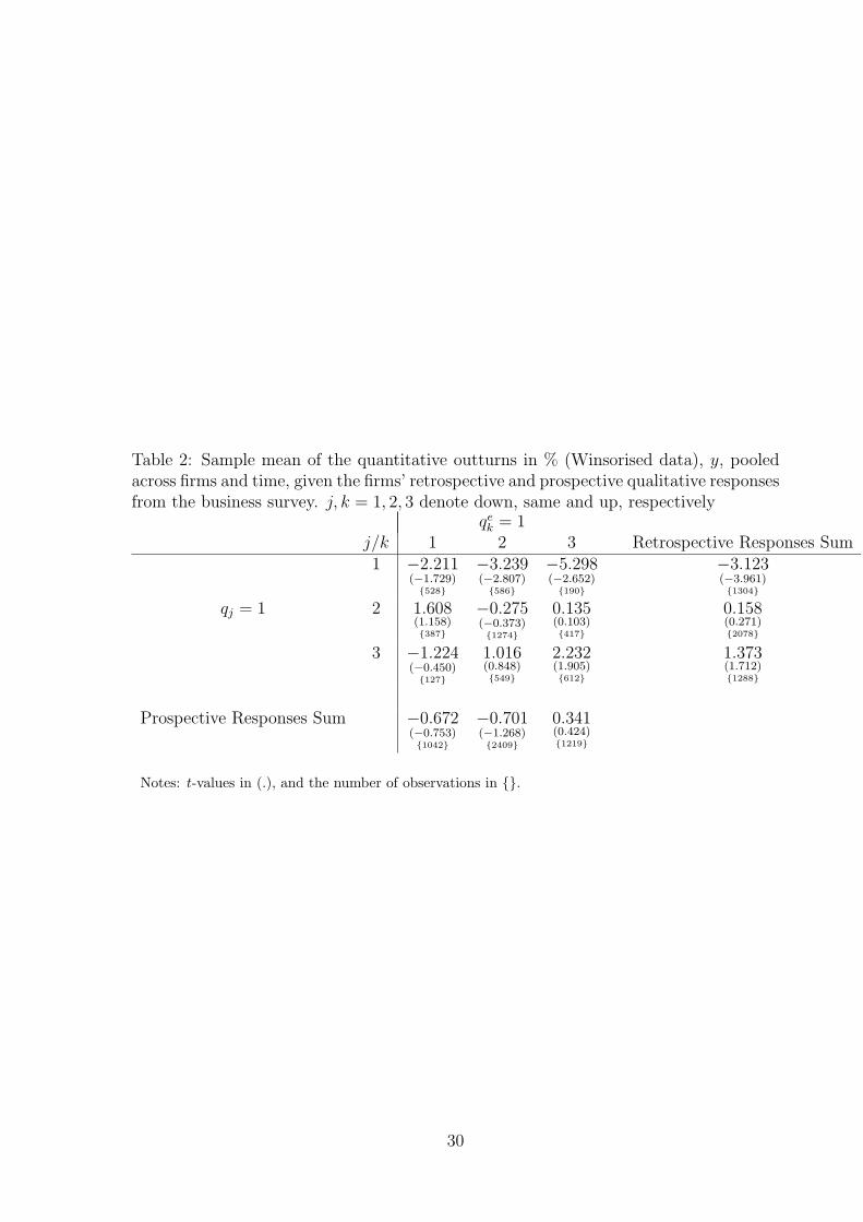
reported. Table 2 then reports analogous results when y is Winsorised to mitigate the
effect of outliers. In these tables the weighted (by the number of observations) sum of
the sample means across a given row (or column) gives the sample mean of y for each
Inspection of these row and column sums indicates that only retrospectively do the
sample means increase with j. We should expect them to increase if the retrospective
qualitative business data are “coherent” with the quantitative outturns. Looking first
at the raw data in Table 1, when firms retrospectively reported a ‘down’ in fact they
contracted, on average, as revealed by the quantitative data, by −4.0%. When they
reported an ‘up’ they grew by 2.7%. And when they reported ‘no-change’ they contracted
very slightly (−0.1%). But one cannot reject the null hypothesis that in fact output
growth was zero even at a 1% significance level, with a t-ratio of −0.145. Even assuming
all firms have the same thresholds, further assumptions about the objective density for
y would be needed before inference about the sign of the thresholds, b1 and b2, could be
drawn from the results in Table 1 alone.
Carrying out pairwise t-tests to test (19) also reveals these differences between the
sample means to be statistically significant at a 5% significance level. In particular,
the t-value testing equality of the sample means for those firms reporting a ‘down’
and an ‘up’ is 3.90 (implying a 1-sided p-value of 0.0%). There remain pronounced
differences between the sample means of those firms reporting a ‘down’ or an ‘up’ when
there was an additional holiday to celebrate the Queen’s Jubilee. The 2002 (Football) World Cup isalso believed to have distorted the typical seasonal pattern. In any case, this oddity in the industrialproduction data does not affect our analysis below which is based on the underlying firm-level data.The aggregate data are considered only for reference purposes.
20
compared with those firms reporting ‘no-change’. The associated t-values are 2.56 and
1.87, respectively, implying (1-sided) p-values of 0.5% and 3%. This also implies rejection
of the joint null hypothesis in (19), after applying the Bonferroni correction. Therefore,
overall the retrospective survey data do contain a signal about the quantitative data. A
similar picture is seen using the Winsorised data in Table 2, although the sample means
do not increase so strongly with j.
But the expectational survey data do not contain a statistically significant signal
about the quantitative outturns, y. Firms that expected a ‘down’ did, on average, in
fact subsequently contract, as revealed by the quantitative data, but only by −1.0% as
seen in Table 1, and −0.67% as shown in Table 2. This contrasts with the much larger
contractions (of −4.0% and −3.1%) in firms that reported ‘a down’ retrospectively. In
turn, firms that expected an ‘up’ did subsequently grow, but again quite modestly at
1.4% and 0.34% in Tables 1 and 2, respectively. These sample means, for the expecta-
tional data, are also poorly determined (with large standard errors) such that one cannot
reject the null hypothesis of noise, (17), using information contained in both Tables 1
and 2. For example, focusing on the (pairwise) test of equality of the sample means for
those firms that expected a ‘down’ and those that expected an ‘up’ we find t-values in
Tables 1 and 2 of 1.27 and 0.84, respectively.
Macroeconomic shocks, occurring after the forecast was made, might be thought to
contribute to our finding that the expectational data do not contain a signal about the
subsequent quantitative outturns; although they do not appear to prevent the expec-
tational data being best-case predictions for the qualitative outcome data, as shown in
Sections 6.1 and 6.2. We did re-compute Tables 1 and 2 having subtracted macroe-
conomic forecasts, based on recursive estimation of an autoregressive model estimated
using real-time data vintages available from the ONS, from y and inference was qualita-
tively unchanged. This is unsurprising, given the absence (see Figure 4) of pronounced
(aggregate) cyclical movements in this stable sample. The ex post macroeconomic fore-
casting errors observed over this sample period average out to zero.
6.4 An apparent paradox
To summarise, our analysis of the firm-level qualitative and quantitative data has re-
vealed that:
i.) the firm-level qualitative expectational data are best-case predictions of the out-
comes but, importantly, the ‘outcomes’ as declared qualitatively by firms;
21
ii.) the retrospective qualitative data and the quantitative outcome data from the two
different surveys are coherent with each other;
iii.) the qualitative expectational data are not consistent with what we should expect
if they were best-case predictions of the quantitative outturns; they do not even
contain a signal about the quantitative outcome data.
This is an apparent paradox. Given i.) and ii.) hold we might expect this to imply
that the qualitative expectational data should be useful at explaining the quantitative
outcome data, contradicting our finding in iii.). While of empirical significance, we
explore two possible explanations for this apparent paradox.
Firstly, the accumulation of ‘forecasting’ errors and ‘discretisation’ errors mean the
ability of the qualitative expectational data to predict the quantitative outcome data
can be drowned out by the combination of these two noise terms. This can be seen by
defining the two errors as follows:
E(y | qk = 1) = E(y | qek = 1) + uk (20)
y = E(y | qk = 1) + udk (21)
where the ‘forecasting’ error, uk, defined in (20), is the difference between firms’ retro-
spective qualitative assessment of their output growth and firms’ qualitative forecast and
reflects how firms’ update their (qualitative) forecast having observed y. The ‘discretisa-
tion’ error, udk, is the difference between the outcome, y, and firms’ qualitative assessment
of it. Assuming a normal distribution for y this can be written like a generalised residual
(see Gourieroux et al. (1987)) so that6
udk = y − φ(ak−1)− φ(ak)
Φ(ak)− Φ(ak−1)(22)
where φ(.) denotes the density and Φ(.) the distribution function of the standard normal
distribution. udk reflects how much information is lost through firms reporting qk rather
than y. Discretisation of (the continuous) y reduces the amount of information in the
sense defined by Shannon (1948). Less information would be lost if the number of states
6The normality assumption is innocuous given our use of nonparametric tests. We make it here forexpositional purposes only. The point we wish to make is that an error is induced, and informationlost, when then the quantitative data are reduced to a qualitative response. A different distributionalassumption for y would affect the form ud
k takes but not eliminate it.
22
into which y was discretised was greater than three (k = 1, 2, 3). Substituting (20) into
(21) then reveals that
y = E(y | qek = 1) + uk + ud
k (23)
implying that the informational content of firms’ qualitative expectations is weakened
by the compounding of the two errors.7
Our results therefore provide firm-level motivation for the method introduced by
Lee (1994) to account for this discretisation error when using expectational data at
the aggregated/macroeconomic level. Lee (1994) finds that the evidence against the
rationality of aggregated expectational data, from the CBI survey, is weaker when one
conducts rationality tests based on uk (aggregated across firms) alone, rather than using
the composite error (udk + uk). Similarly, we find that adding the discretisation error to
the forecasting error renders the qualitative expectational data uninformative about the
quantitative outcome data at the firm-level.
Secondly, firms may not reply to the expectational question with the conditional
mean E(y | qek = 1) of their subjective density forecast in mind. They may use the mode
or median instead. When they form best-case predictions in this manner i.) should
hold. But the qualitative expectational data need not be best-case predictions of the
quantitative outturns and need not contain a signal about them - as long as the mean
forecast does differ from the mode/median. They will differ when there are pronounced
asymmetries/multi-modalities in firms’ conditional density forecasts. But ii.) should
continue to hold given that retrospectively firms do not base their qualitative response
on their subjective density forecast. Instead they are supposedly replying by stating the
category qk = 1 (k = 1, 2, 3) in which y is contained.
From a practical perspective these results suggest that qualitative business survey
data, given that they are published ahead of the ONS’s quantitative data, are likely to
prove more useful for nowcasting than forecasting. But it is possible that aggregation
of firm-level expectational data improves the informational content of macroeconomic
indicators constructed from these expectational data. Forecasting and discretisation
errors may be offsetting. Certainly, as argued by Mitchell et al. (2005), more attention
should be devoted to how qualitative expectational data are quantified and aggregated.
The widely used “balance of opinion” is but one option. Nevertheless, it would have been
reassuring for those using the aggregated expectational data if we had found that the
7Rationality requires the discretisation error, udk, and uk to be mean zero and serially uncorrelated,
and orthogonal to information known at the time the firm formed its expectation.
23
firm-level expectational data contained a signal about the quantitative outcome data.
7 Conclusion
Qualitative expectational data from business surveys are widely used to construct fore-
casts on the assumption that they are forward-looking and say something useful about
what will happen to the economy in the future. But, based typically on evaluation at
the macroeconomic level, doubts persist about the utility of these data. In this paper we
evaluate the ability of the underlying firm-level expectations to anticipate subsequent
outcomes. Importantly this evaluation is not hampered by only having access to quali-
tative outcome data obtained from subsequent business surveys. Quantitative outcome
data from official surveys are also exploited. This required access to a panel dataset, for
UK manufacturing firms, which matches firms’ responses from the qualitative business
survey with these same firms’ quantitative replies to a different survey carried out by
the national statistical office.
We use and develop nonparametric tests for the rationality of the firm-level qualita-
tive expectational data. Rationality tests remain a useful tool in evaluating the utility
of expectational data. This is because under rationality outcomes do not differ system-
atically from what was expected. But to test the rationality of qualitative expectations
data requires auxiliary assumptions to be made, which are tested jointly with rationality.
We therefore follow Manski (1990) and Das et al. (1999) and refer to the tests as tests
of the “best-case scenario”. In particular, we discuss how the implications of rationality
depend on the firm’s loss function. Under rationality, different loss functions result in
different categorical predictions, given the firm’s subjective density forecast. We there-
fore follow Das et al. (1999) and conduct tests when firms report the mode, the median
(more generally the alpha-quantile) or the mean of their subjective density forecast of
future output growth. When firms have the mode or median of their subjective density
in mind, tests of the best-case scenario exploit the (retrospective and prospective) qual-
itative business survey data only. But when they have the mean in mind, tests require
knowledge of the quantitative outcome data.
As well as testing the ability of the expectational data to forecast the two distinct
outcome variables, we test what we call the coherence between these qualitative and
quantitative outcome measures. This involves testing whether the two outcome variables
are measuring the same concept of output growth, as implicitly assumed when outcome
data from qualitative business surveys are used to provide a contemporaneous indication
24
(nowcast) of economic activity.
The tests reveal an apparent paradox. Despite evidence that the qualitative and
quantitative outcome data are coherent, we find that the expectational data offer ratio-
nal forecasts of the qualitative but not the quantitative outcomes. One explanation is
that firms do not reply to the expectational question with the conditional mean of their
subjective density forecast in mind. Another candidate explanation is that ‘discretisa-
tion’ errors, explained by the qualitative nature of the expectational data, drown out
the ability of the expectational data to predict the quantitative outcome data.
In summary, our firm-level findings therefore suggest that:
1. Qualitative business surveys are likely to prove more useful for nowcasting than
forecasting.
2. Business surveys might be of more value for forecasting if the questions in the
survey were modified to ask for quantitative expectational data.
(a) It would also help if the survey were explicit about what ‘feature’ of their
subjective density forecast firms should report. At present some may report
subjective means, others modes or medians. Indeed if their loss function is
asymmetric they may report various quantiles. We have seen that the feature
reported can affect the utility of the survey.
(b) But ideally business surveys would ask for probabilistic information in the
form of a density forecast. Some surveys of professional forecasters already
supply this information, as discussed above. Forecasts can then be used -
compared and evaluated - independently of firms’ loss functions; see Diebold
et al. (1998) and Mitchell & Wallis (2010). Point forecasts also reveal nothing
about the uncertainty that firms feel. Comparisons can also be made between
the point forecasts and the subjective density forecasts; see Engelberg et al.
(2009) and Clements (2009, 2010).
Future work might test the utility of expectational data at the firm-level both for
different sectors and for other countries using the methods we set out. This may require
the permission of the survey producers. As in the UK, the qualitative and quantitative
surveys are often carried out by different institutions. But further applications at the
firm-level would be helpful in establishing whether or not our results, for UK manufac-
turing, are shared by expectational data more generally.
25
2001 2002 2003 2004 2005
25
50
Pessimists: p.1p11 p21 p31
2001 2002 2003 2004 2005
20
40
60 No−change: p.2p12 p22 p32
2001 2002 2003 2004 2005
20
40
60Optimists: p.3p13 p23 p33
Figure 2: Estimates of pjk = Pr(qj = 1 | qek = 1) (in percentages), where j, k = 1, 2, 3
denote down, same and up, respectively.
26
2001 2002 2003 2004 2005
0.3
0.4
0.5
0.6
0.7
0.8 Pessimists: p.1p21+p31
2001 2002 2003 2004 2005
0.4
0.5
0.6
0.7
0.8 Optimists: p.3p13+p23
2001 2002 2003 2004 2005
0.2
0.3
0.4
0.5No−change: p.2
p12
2001 2002 2003 2004 2005
0.2
0.3
0.4
0.5No−change: p.2
p32
Figure 3: 90% confidence intervals for the cumulative probabilities ( 11) and (12) usedto test median expectations
27
2001 2002 2003 2004 2005
0.15
0.20
0.25
0.30
0.35
Realisation higher than expected Realisation lower than expected
2001 2002 2003 2004 2005
−2
−1
0
1T−test for equality of the two proportions
95% critical value
2001 2002 2003 2004 2005
−5
−3
−1
1
3
5 Industrial production (3 month growth rate in %)
Figure 4: The top panel shows the proportion of firms who, when looking at the medianof their predictive density, were too optimistic or too pessimistic when forecasting. Themiddle panel reports t-tests for the equality of these two proportions based on (14). Thebottom panel shows the growth rate of (aggregate) industrial production.
28
Table 1: Sample mean of the quantitative outturns in % (raw data), y, pooled acrossfirms and time, given the firms’ retrospective and prospective qualitative responses fromthe business survey. j, k = 1, 2, 3 denote down, same and up, respectively
qek = 1
j/k 1 2 3 Retrospective Responses Sum1 −2.689
(−1.268){528}
−4.790(−2.757)
{586}
−5.401(−2.157)
{190}
−4.028(−3.312){1304}
qj = 1 2 2.304(0.976){387}
−0.946(−0.836){1274}
0.091(0.045){417}
−0.132(−0.145){2078}
3 −4.087(−1.127)
{127}
2.414(1.314){549}
4.444(2.389){612}
2.738(2.217){1288}
Prospective Responses Sum −1.005(−0.690){1042}
−1.115(−1.320){2409}
1.420(1.155){1219}
Notes: t-values in (.), and the number of observations in {}.
29
Table 2: Sample mean of the quantitative outturns in % (Winsorised data), y, pooledacross firms and time, given the firms’ retrospective and prospective qualitative responsesfrom the business survey. j, k = 1, 2, 3 denote down, same and up, respectively
qek = 1
j/k 1 2 3 Retrospective Responses Sum1 −2.211
(−1.729){528}
−3.239(−2.807)
{586}
−5.298(−2.652)
{190}
−3.123(−3.961){1304}
qj = 1 2 1.608(1.158){387}
−0.275(−0.373){1274}
0.135(0.103){417}
0.158(0.271){2078}
3 −1.224(−0.450)
{127}
1.016(0.848){549}
2.232(1.905){612}
1.373(1.712){1288}
Prospective Responses Sum −0.672(−0.753){1042}
−0.701(−1.268){2409}
0.341(0.424){1219}
Notes: t-values in (.), and the number of observations in {}.
30
References
Abberger, K. (2007), ‘Qualitative business surveys and the assessment of employment –
a case study for germany’, International Journal of Forecasting 23(2), 249–258.