Working papers are in draft form. This working paper is distributed for purposes of comment and discussion only. It may not be reproduced without permission of the copyright holder. Copies of working papers are available from the author.
The Value of a "Free" Customer
Sunil Gupta Carl F. Mela Jose M. Vidal-Sanz
The Value of a "Free" Customer
Sunil GuptaCarl F. Mela
Jose M. Vidal-Sanz1
August 23, 2006
1Sunil Gupta ([email protected]) is a Professor of Business Administration, Harvard Business School,Soldiers Field, Boston, Massachusetts 02163. Carl F. Mela ([email protected]) is a Professor of Marketing,The Fuqua School of Business, Duke University, Durham, North Carolina, 27708. José M. Vidal-Sanz (jvidal@ emp.uc3m.es) is an Assistant Professor of Marketing, Universidad Carlos III, Calle Madrid 126, 28903Getafe (Madrid), Spain.
Abstract
Central to a firm’s growth and marketing policy is the revenue and profit potential of its customerassets. As a result, there has been a recent proliferation of work regarding customer lifetime value.However, extant research in this area is silent regarding how to assess the profitability of customersin a networked setting. In such settings, the presence of one type of customer can affect the value ofanother. Examples of such settings include job agencies (whose customers include both job seekersand listers), realtors (whose clients include home sellers and purchasers), and auction houses (whosecustomers include buyers and sellers). Customers such as buyers of an auction house pay no feesto the firm making their value difficult to compute. Yet these customers generate value to the firmbecause their presence attracts fee-paying sellers. In this paper we consider the value of a customerin these types of networked setting.
We compute the value of customers by developing a joint model of buyer and seller growth. Thisgrowth comes from three sources — marketing actions (price and advertising), direct network effects(e.g., buyer to buyer effects), and indirect network effects (e.g., buyer to seller effects). Using thisgrowth model we concurrently solve the firm’s problem of choosing optimal pricing and advertisingsubject to constraints on customer growth. By relaxing constraints on growth by one customer,we can then impute their lifetime value to the firm. We apply our model to data from an auctionhouse.
Our results show that there are strong direct and indirect network effects present in our data.We find that in the most recent period buyers have a value of about $550 and the sellers have avalue of around $500. We also find that our approach leads to estimates of firm value that are moreaccurate than models that fail to consider network effects. Finally, price and advertising elasticitiesare low (-0.16 and 0.006) and decrease over time as network effects become increasingly important.
Metrics of customer value are becoming more important as firms are increasingly compelled to
justify the role of marketing investments on firm profitability (Marketing Science Institute 2006).
A central metric for assessing the profitability of customers is customer lifetime value (CLV); the
present value of all future profits generated by a customer (Kamakura et al. 2005). Using CLV a firm
can rank order its customers or classify them into tiers based on their expected profitability. This
allows firms to appropriately allocate resources across high versus low value customers (Reinartz
and Kumar 2003, Rust, Lemon and Zeithaml 2004, Venkatesan and Kumar 2004). CLV can also be
used for making customer acquisition decisions such that a firm does not spend more on acquiring
a customer than the CLV of that customer (Gupta and Lehmann 2003, Gupta and Zeithaml 2006).
It allows firms to balance their resources between customer acquisition and customer retention
(Reinartz, Thomas and Kumar 2005). Recent studies also show that CLV can provide a link
between customer value and firm value (Gupta, Lehmann and Stuart 2004).
Current models of CLV, however, omit an important element. Consider the case of Monster.com,
an employment market place where job-seekers post their resumes and firms sign up to find potential
employees. Monster provides this service free to job-seekers and obtains revenue by charging fees
to the employers. A natural question arising from this business model is how much Monster should
spend to acquire a job-seeker. Traditional models of CLV can not answer this question since job-
seekers do not provide any direct revenue. In fact, if one includes the cost of maintaining resumes,
the standard CLV for a job-seeker is negative. However, without job-seekers employers will not sign
up, and without these firms Monster will have no revenues or profits. In other words, the value of
job-seekers is through their indirect network effect on job listers.1 This indirect network effect is
not limited to employment services only (e.g., Monster, Hotjobs, Craiglist) but also extends to any
exchange with multiple buyers and sellers (e.g. eBay, real estate).
The purpose of this study is to assess customer value when two parallel populations (e.g.,
buyers and sellers) interact and have strong 1) direct (within population) and 2) indirect (across
populations) network effects. In these situations typically one set of customers (e.g., sellers) provide
direct financial returns to the company. For example, sellers provide commissions to real estate
1Such markets are denoted as two-side matching markets in Sociology and Economics (Demange and Gale 1985).Our emphasis differ from this work inasmuch as we are not as concerned with matching specific employers withprospects as we are with understanding how the presence of one of these populations attracts the other.
1
agencies. However, firms must acquire and maintain the other set of customers (e.g., buyers).
These customers are "free" as they do not provide any direct revenue. Our objective is to develop
a model to assess the value of both types of customers.2 This should enable us to answer the
following questions:
• Are direct and indirect network effects sizable in practice? If so, this suggests the potential
for large firms with strong network effects to dominate markets as the network grows.
• How much should a company spend to acquire new customers in the presence of these networkeffects? For example, how much should Monster spend on acquiring an additional job-seeker,
how much should PayPal spend on acquiring a new account, how much should a dating service
spend for a new client, how much should an auction house spend to acquire a new buyer? In
other words, how much should a company spend on acquiring a "free" customer who does not
provide any direct financial returns to the firm. This question is key to firms that operate in
markets with strong direct and indirect network effects.
• How does the value of a customer change over time? Since the magnitude of network effectsis likely to be time-dependent, customer value should also change over time. This suggests
that the maximum amount of money that a firm should spend on a "free" customer changes
over the life of a company. Once again, existing models of CLV do not address this dynamic
aspect.
• How do we apportion value between buyers and sellers? In other words, how much of the
value arising from the exchange between buyers and sellers accrues from each set of customers?
Currently, firms have no metrics to apportion these revenues or profits. Some firms apportion
all value to sellers since they generate the revenues. However, this clearly understates the
value of buyers. Others use an arbitrary rule of thumb (e.g., 50-50) to split the profits between
buyers and sellers. However, this implicitly assumes that both parties are equally important,
which may not be necessarily correct. Finally, the network effects of buyers and sellers are
likely to be different. This suggests that the proportion of value allocated between buyers
and sellers may also change over time.
2Throughout the paper we will use the terms buyers and sellers for the two parallel population of customers.
2
• How should firms’ marketing efforts change over time in the presence of network effects? Howdo customers’ sensitivities to these marketing actions change over time? Marketing actions
may be more critical in the early stages and network effects may dominate in later stages
of a firm’s life cycle. It is worth noting that extant CLV models fail to account for the
role customer acquisitions play on subsequent marketing spending. As the market saturates,
for example, optimal marketing spend may decrease even in the absence of network effects.
Hence, there is an indirect link between customer acquisition and marketing spend, and this
should logically affect customer valuation.
• Does the omission of network effects understate the value of customer base and hence thevalue of a firm? For example, Gupta et al. (2004) found that eBay’s customer value is
significantly lower than its market value. They speculate that this difference may be due to
the omission of indirect network effects from their model.
While economists and marketing researchers have studied network effects in many contexts (e.g.,
Katz and Shapiro 1985, 1986, Neil, Kende and Rob 2000, Gupta, Jain and Sawhney 1999, Yao and
Mela 2006), none of these studies examined the impact of these network effects on customer value.
One recent study estimated the value of a lost customer by accounting for the word-of-mouth or
direct network effects and found these effects to be very large (Hogan, Lemon and Libai 2004).
However, we are not aware of any study that examines customer value when there are strong direct
and indirect network effects. The indirect network effects are especially important in the buyer-
seller contexts that we study here. Modeling these effects are crucial to assess the value of "free"
customers who do not provide any direct revenue to the firm.
The paper proceeds as follows. We begin by developing a model that captures the growth of
buyers and sellers from three sources — marketing actions (price and advertising), direct network
effects or word-of-mouth, and indirect network effects. Next we define the firm’s problem as an
optimal control problem wherein the firm chooses its marketing actions to maximize its long run
profits subject to the growth of these populations. These growth constraints imply costates or
Lagrangian multipliers for the optimization problem yielding the incremental profits to a firm
arising from an additional buyer or seller; that is, the lifetime value of that incremental seller or
buyer to the firm. We apply our model to data obtained from an auction house, and estimate the
3
model using a Generalized Method of Moments based on both the growth and the Euler equations.
This estimation approach explicitly accounts for endogeneity of marketing actions and increases
the efficiency of the model estimates. We use the resulting parameter estimates to address the
managerial questions highlighted above. We then conclude with limitations and next steps.
2 A Model of Customer Value in the Presence of Network Effects
2.1 Customer Growth and Network Effects
Consider two parallel populations of buyers and sellers. The acquisition of customers in each group
can be captured by a "diffusion-type" model as follows:3
·NB
t =
µa(At) + b
0NBt
MB+ g
NSt
MS
¶¡MB −NB
t
¢− r(NBt ) (1)
·NS
t =
µα(pt) + β0
NSt
MS+ γ
NBt
MB
¶¡MS −NS
t
¢− ρ(NSt ) (2)
where NBt and N
St are the number of buyers and sellers at time t,
·NB
t and·NS
t denote the derivatives
or the net customer acquisition rate of buyers and sellers, MB and MS are the potential market
size of buyers and sellers, At is the advertising spending at time t and pt is the price firm charges
its sellers at time t. Some of the key characteristics of this system of equations are as follows:
1. The term a(At) recognizes that a firm can accelerate the growth of its buyers through ad-
vertising. In our application of the e-auction house this takes the form of television and
internet advertising. Consistent with prior literature (e.g., Horsky and Simon 1983), we fur-
ther assume that a(At) = x+ h lnAt. In other words, there are diminishing marginal returns
from advertising and the coefficient h determines buyers’ responsiveness to firm’s advertising.
Advertising is a decision variable for the firm and it can change over time. In our data (see
Section 3), advertising is the only marketing variable on the buyer side.
2. Similarly, the term α(pt) highlights the fact that the growth of sellers depends on the price
the firm charges them. Once again, price is a decision variable and it can change over time.
3Similar models have been previously used in the context of international diffusion of products (Kumar andKrishnan 2002).
4
We assume that α(pt) = φ − θ ln pt. Here the parameter θ indicates sellers’ sensitivity to
firm’s pricing. In our data, price is the only marketing variable available on the seller side.
3. The direct network or word-of-mouth effect for buyers and sellers is captured by the second
term in equations (1) and (2). This formulation is consistent with the diffusion literature.
Hogan, Lemon and Libai (2003) used a similar term to capture the direct network effect
of losing a customer. The value of the parameters b0 and β0 indicate the strength of direct
network effects. These may be positive as a result of word of mouth, or negative as a result
of a crowding phenomenon where, all else equal, a buyer (or seller) prefers less competition.
4. As a firm acquires more buyers it becomes more attractive for sellers to join the firm as well.
The reverse is also true — the more sellers a firm has, the more buyers it is likely to attract.
This indirect network effect is captured by the third term in equations (1 and 2). The value
of the parameters g and γ indicate the strength of indirect network effects.
5. Unlike the traditional diffusion models, in our context customers can also leave a firm. Cus-
tomer defection is captured by the terms r(NBt ) and ρ(NS
t ). In particular, the number of
customers who defect a firm is proportional to the number of current customers, and the pa-
rameters r and ρ denote the rate of defection. Some studies exogenously specify the defection
rate (Gupta et al. 2004, Peres, Libai and Muller 2006). Alternatively, one can assess the net
impact of acquisition and defection by reformulating the above equations as follows:4
·NB
t =
µa(At) + b
NBt
MB+ g
NSt
MS
¶¡MB −NB
t
¢(3)
·NS
t =
µα(pt) + β
NSt
MS+ γ
NBt
MB
¶¡MS −NS
t
¢(4)
Here the parameter b and β capture the net effect of acquisition through word-of-mouth
and defection through customer dissatisfaction. A negative value for these parameters will
indicate that customer defection is greater than the word-of-mouth effect (or possibly that
all else equal, sellers and buyers prefer less competition).
4 In principle it is possible to estimate b0 and r (and similarly β0 and ρ) separately. However, it is easy to show
that when (MB−NB
t )MB ≈ 1, b = b0 + r, thus making it difficult to estimate b0 and r separately. In our data, estimates
of (MB−NB
t )MB average about 0.9 and (
MS−NSt )
MS averages about 0.85. Given these are close to 1.0, we were unable toseparately identify b0 and r in (1) and (2). Therefore we rely on the formulation given by (3) and (4) in our subsequentmodeling discussion.
5
2.2 Optimal Marketing Policies and Customer Value
Equations (3) and (4) characterize the growth of buyers and sellers as a result of firm’s actions
(advertising and pricing), word-of-mouth or direct network effects as well as indirect network effects
where an increase in the number of buyers makes it more attractive for sellers to join the firm and
vice versa. The objective of the firm is to choose its advertising and pricing policies in such a fashion
that they maximize its long run profits. More formally, the objective function of the company is:
maxpt,At,NB
t ,NSt
Z ∞
0
¡mt (pt) N
St −At
¢e−it dt (5)
subject to the growth equations (3) and (4) and initial conditions NB0 = N
S0 = 0. Here the control
variables are pt and At, and the state variables are NBt and NS
t . Further, mt (pt) = pt − ct is themargin, pt is the price and ct is marginal cost at time t. The discount rate for future profits is i.
We would like to highlight a few characteristics of equation (5). First, the profits for the company
depend directly on the number of sellers and the price the firm charges them. If there is no indirect
network effect of buyers on sellers, the number of buyers is irrelevant for profit maximization. In
such a situation a firm has no reason to spend any money on buyer-oriented advertising and it
has no way of assessing the long-term value of a buyer. This highlights the importance of indirect
network effects in our context. Second, this formulation is consistent with the concepts of CLV
and customer equity since it explicitly accounts for the long run profitability of current and future
customers. Third, unlike most CLV models, this equation suggests that firm’s actions (price and
advertising) can influence customer growth and hence the overall value of the firm. In other words,
price and advertising decisions are dynamic and endogenous. As a result, they are affected by
customer acquisitions and should therefore be considered when computing CLV.
If we define G¡t,NB
t ,NSt , pt, At
¢to be the profit function (i.e., the terms within the integral)
in equation (5), gB¡A,NB, NS
¢to be the acquisition rate of buyers as given by equation (3) and
gS¡p,NB, NS
¢to be the acquisition rate of the sellers as indicated in equation (4), then the profit
maximization of equation (5) becomes a standard optimal control problem whose solution can be
determined by Pontriagyn’s maximum principle (see Appendix A1). To solve this problem we form
6
the following Hamiltonian function
H¡t,NB,NS , p, A,λB,λS
¢= G
¡t,NB, NS, p,A
¢+ (6)
λBgB¡A,NB, NS
¢+ λSgS
¡p,NB, NS
¢,
where λB,λS are auxiliary or costate variables. The solution to this optimal control problem
satisfies the conditions indicated in Appendix A1.
The costates can be interpreted as Lagrangian multipliers. In the optimal solution, λBt provides
the customer value of an incremental buyer acquired at time t over an infinite horizon, i.e. the
effect of an additional buyer on the long-term discounted profit of the company. Analogously, λSt
provides the customer value of an additional seller acquired at time t. Further, the value of an
additional buyer or seller is allowed to vary over time. This intuitively makes sense as one might
expect the network effects to vary over the lifecycle of the company. For example, in the early
stages of a company, marketing actions may be more important to attract customers, while in the
growth phase direct and indirect network effects may dominate. In other words, our model will
allow us to find out the maximum amount of money a firm should spend to acquire a "free" buyer
— something that traditional CLV models can not address. Further, we will also be able to show
how this maximum acquisition cost varies over time.
2.3 Model Estimation
2.3.1 Customer Growth Model
For estimation purposes we make two adjustments to our model presented in equations (3) and
(4). First, our data are in discrete time so the model formulation is changed accordingly. Second,
an estimation error is included. These modifications are typical in empirical estimation of diffusion
type models. Consequently, the customer growth model for estimation purposes becomes:
NBt+1 −NB
t =
µx+ h lnAt + b
NBt
MB+ g
NSt
MS
¶¡MB −NB
t
¢+ et, (7)
NSt+1 −NS
t =
µφ− θ lnPt + β
NSt
MS+ γ
NBt
MB
¶¡MS −NS
t
¢+ εt (8)
In the past, these growth models have often been estimated using OLS, nonlinear least squares,
seemingly unrelated regressions or similar approaches. In many cases the purpose of the model
estimation was simply to assess the impact of a marketing variable on the diffusion process. For
7
example, Simon and Sebastian (1987) investigate the impact of advertising on the diffusion of
new telephones in West Germany. These studies are descriptive in nature and do not attempt to
provide optimal advertising or pricing policies that maximize firm’s profits. In our context this is
problematic as we seek to assess the impact of demand on firm profits in order to infer CLV. This
necessitates an analysis of the firm’s decisions of price and advertising, which we consider next.
2.3.2 Firm’s Price and Advertising Decisions
Studies that combine empirical estimation of diffusion-type models with analytical models of profit
maximization and optimal marketing policies of the firm typically do it in two stages. In the first
stage these studies ignore the optimal control problem of the firm and use the actual prices and
advertising of the firm as exogenous variables when estimating the growth model of demand. In
the second stage, they "plug-in" the parameter estimates of price and advertising in the optimal
solutions of advertising and price to arrive at the optimal path for these decision variables and
compare the optimal and actual values (e.g., Horsky and Simon 1983, Kalish 1985, Chintagunta
and Vilcassim 1992, Chintagunta and Rao 1996). A third set of studies explore the dynamic policies
in a purely theoretical fashion using the solutions of the optimal control problem and examining
the comparative statics or using numerical illustrations (e.g., Feichtinger, Hartl and Sethi 1994,
Thompson and Teng 1984, Horsky and Mate 1988, Dockner and Jorgensen 1988).
All these approaches have significant limitations in the context of CLV. Theoretical approaches
provide directional results but are not very useful if the objective is to provide empirical estimates
in a particular application. The empirical approaches used in the past have two major drawbacks.
First, the estimation of the diffusion equations assumes price and advertising to be exogenous. If
the objective of the firm is to find the optimal price and advertising policy then these marketing
actions by definition depend on the customer growth. In other words, marketing activities should
be endogenous. One ramification of this observation is that acquisition of a customer may increase
the network effect which in turn may reduce the firm’s marketing cost. As such, marketing spend
should have an indirect affect on customer value. In principle this endogeneity issue can be solved
by using an instrumental variable approach. However, this only solves half of the problem. The
second drawback of the traditional approaches is that the first stage estimation of the diffusion
model is completely divorced from the second-stage "plug-in" analysis of the firm’s optimal control
8
problem. This second-stage analysis is necessary to make inferences about customer profitability
as it yields information needed to compute the Lagrangians which yield the measures of buyer and
seller CLV.
Therefore, we propose an estimation method that treats firm’s actions (price and advertising)
as endogenous and at the same time considers firm’s objective function of maximizing long run
profits. Specifically, the firm solves the following discrete time problem:
maxpt,At
E0
" ∞Xt=0
(1 + i)−t¡NSt Spt −At
¢#
s.t.
NBt+1 = NB
t +
µx+ h lnAt + b
NBt
MB+ g
NSt
MS
¶¡MB −NB
t
¢+ et (9)
NSt+1 = NS
t +
µφ− θ ln pt + β
NSt
MS+ γ
NBt
MB
¶¡MS −NS
t
¢+ εt
and subject to initial values NS0 = 0, N
B0 = 0. In compact notation, this problem can be expressed
as
maxpt,At
E0
" ∞Xt=0
δtG¡NBt ,N
St , pt, At
¢#
NBt+1 = gB
¡At, N
Bt ,N
St , et
¢(10)
NSt+1 = gS
¡pt, N
Bt , N
St , εt
¢The solution can be expressed by the first-order conditions associated with the following Lagrangian
From the Jacobi-Bellman dynamic programing condition we obtain the following Euler equations
(for details on the derivation see Appendix A2) ,
Et
⎡⎢⎣µ NSt S
θ(MS−NSt )/pt
1h(MB−NB
t )/At
¶+ (1 + i)−1
⎛⎜⎝µ 0
Spt+1
¶+
µD11t+1 D12t+1D21t+1 D22t+1
¶µ NSt+1S
(−θ(MS−NSt+1)/pt+1)
−1h(MB−NB
t+1)/At+1
¶⎞⎟⎠⎤⎥⎦ = 0,(14)
where the D terms are defined in Appendix A2. The system of conditional moments in equation
(14), one for price and the other for advertising, can be denoted by
Et£U¡Ω0, N
Bt , N
St , pt, At,N
Bt+1, N
St+1, pt+1, At+1
¢¤= 0, (15)
where Ω0 denotes the true parameter vector. This implies that for any instrument Zt predetermined
at time t, the unconditional expectations are null, i.e.
E£U¡Ω0, N
Bt , N
St , pt, At, N
Bt+1, N
St+1, pt+1, At+1
¢Zt¤= 0, (16)
10
In addition we have the two moment conditions associated with the dynamics of the state variables
(the growth of buyers and sellers), yielding:
E
∙µNBt+1 −NB
t −µx+ h lnAt + b
NSt
MS+ g
NBt
MB
¶¡MB −NB
t
¢¶Zt
¸= 0, (17)
E
∙µNSt+1 −NS
t −µφ− θ ln pt + β
NBt
MB+ γ
NSt
MS
¶¡MS −NS
t
¢¶Zt
¸= 0, (18)
where Zt includes all the regressors of the model and its lags, as well as some transformations (see
Section (2.3.4) for a description these instruments). It is these four equations (price and advertising
paths, buyer and seller growth models) crossed with each instrument that from the basis of our
estimation equations.
Note, if we ignore the firm’s optimization problem and simply estimate the diffusion models, we
get equations (17) and (18) corresponding to the buyers and sellers. This is the typical approach of
most empirical studies in the past. However, by explicitly incorporating the optimal control problem
of the firm we have additional equations as given by (16). These additional equations provide
structure to the problem and help to identify the model parameters in the empirical estimation.
We use Generalized Method of Moments for parameter estimation (details on the GMM estimation
are provided in Appendix A3).
2.3.4 Discount Rate and Instruments
We assume firm’s monthly discount rate i = 0.015. This monthly discount rate of 1.5% translates
into an approximate annual discount rate of 20%. Given the limited number of variables, we use
two lags for the instruments. The use of lags for instruments is common and as we shall show, these
appear to be good instruments (e.g., Kadiyali, Chintagunta, and Vilcassim 2000). Specifically, Zt
is a 9× 1 vector
Zt =¡1, NS
t−1,NSt−2, N
Bt−1,N
Bt−2, log pt−1, log pt−2, logAt−1, logAt−2
¢0and since we have 4 equations, we use 36 moment equations and 10 parameters (with 26 degrees
of freedom). These instruments are tested via Hansen’s (1982) test of overidentifying restrictions,
or J-statistic (see Appendix A3).
11
3 Application
The application of our model requires information on the number of sellers and buyers over time as
well as the marketing expenditures invested in the acquisition of these customers. An anonymous
auctions house provided monthly data on these quantities for a large market between February 1,
2001 and March 1, 2005. The firm obtains revenues from sellers who list items on its web site for
auction. These revenues are obtained from a listing fee, some promotional fees and a commission on
the sales proceeds; these are combined into an overall margin value by the firm and this is measure
used in our application. If S is the average annual gross merchandise sold per seller, and pt is the
percentage commission charged by the auction house at time t, then firm’s annual margin from
each seller is Spt. The marginal costs in this business are close to zero and therefore we exclude
them from our analysis. The buyers provide no direct revenue to the firm. Not surprisingly the
firm has a greater interest in acquiring and maintaining its sellers even though it recognizes that it
needs to have buyers for its auctions. While sellers push the firm to acquire more and more buyers,
the firm is not sure of how much money to value these buyers — which is the central question of
our research.
The auction house spends money on TV and Internet advertising to attract buyers. The ad-
vertising data were complied quarterly which we converted to monthly data by dividing by three.
In addition, the auction firm provided information on margins and total transacted volume. To
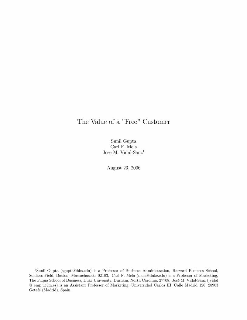
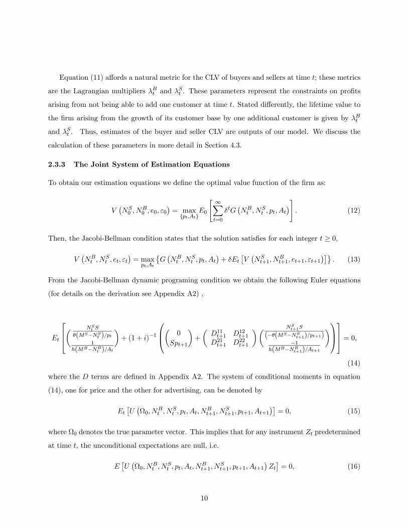
protect the confidentiality of the firm, we are unable to report the specific data means, but in Figure
1 we present information regarding the number of customers and the marketing expenditures over
time, normalized so that the maximum value of each series is one.
The upper left and right panels of Figure 1 indicate rapid growth in the number of buyers and
sellers. There are approximately 4.6 buyers for each seller. The pricing data depicted in the lower
left panel indicates that take rates (margins) are increasing slightly over time, a sign of increasing
pricing power which we speculate may arise from the growth of the buyer-seller network. This
trend suggests it is desirable to account for pricing power and the endogeneity of pricing when
computing the value of a customer. Moreover, the modest change in margins indicate that the
change in seller value over time is not so large that prices change considerably. Advertising, as
indicated by the lower right panel in Figure 1 also shows an increase over time which may be due to
firm’s increasing concern of attracting new buyers over time or it may be due to reduced advertising
12
Figure 1: Changes in Marketing and Demand Over Time
sensitivity in the market prompting the firm to spend more to achieve the same results as before.
In any event, increased spending on advertising is warranted only if buyer value is commensurate
with this investment. These data serve as the basis of our empirical application.
4 Results
4.1 Model Fit
The overall model fit is given by the statistic J = T · QW
³bΩ´, where QW
³bΩ´ is defined inAppendix A3. The J statistics is distributed χ2r−k where r is the number of equations and k the
number of parameters. For our empirical application J = 9.89, r = 36 and k = 10. Therefore
with Prob[χ2(26) > J ] = 0.9982 we accept the overidentifying moment conditions. In other words,
the moment conditions are close to zero and the instruments are orthogonal to the error. The
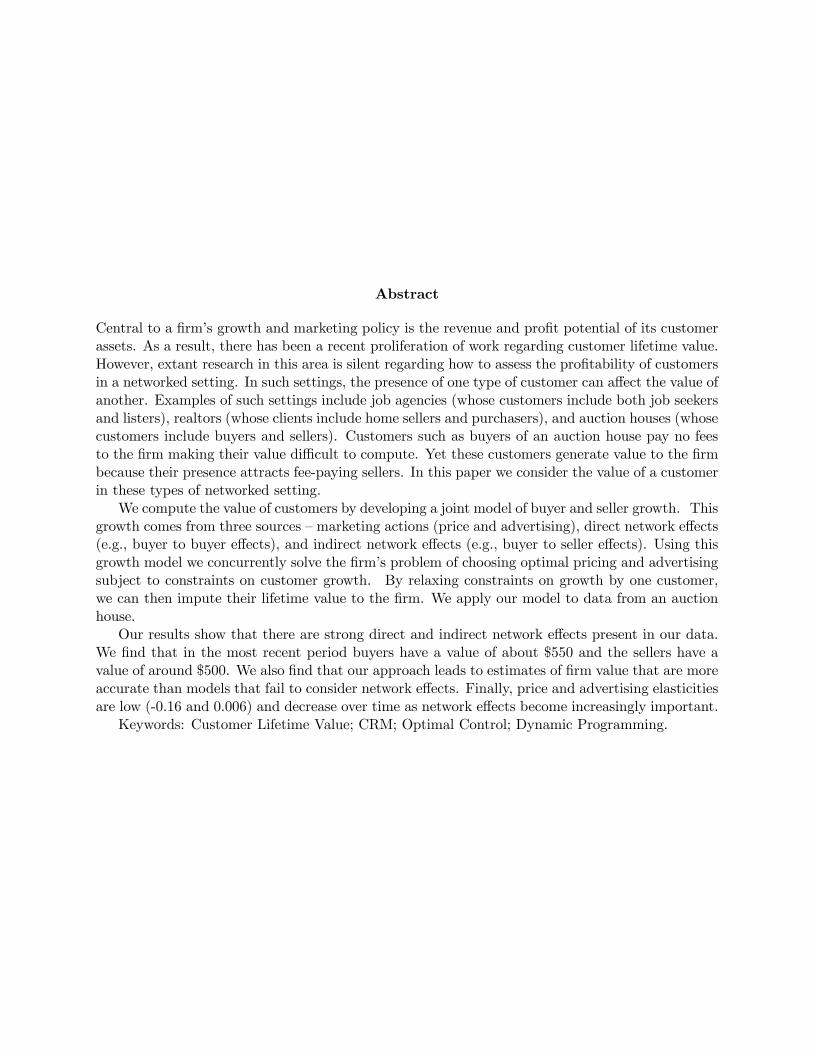
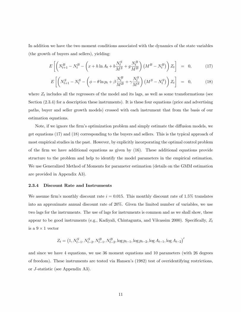
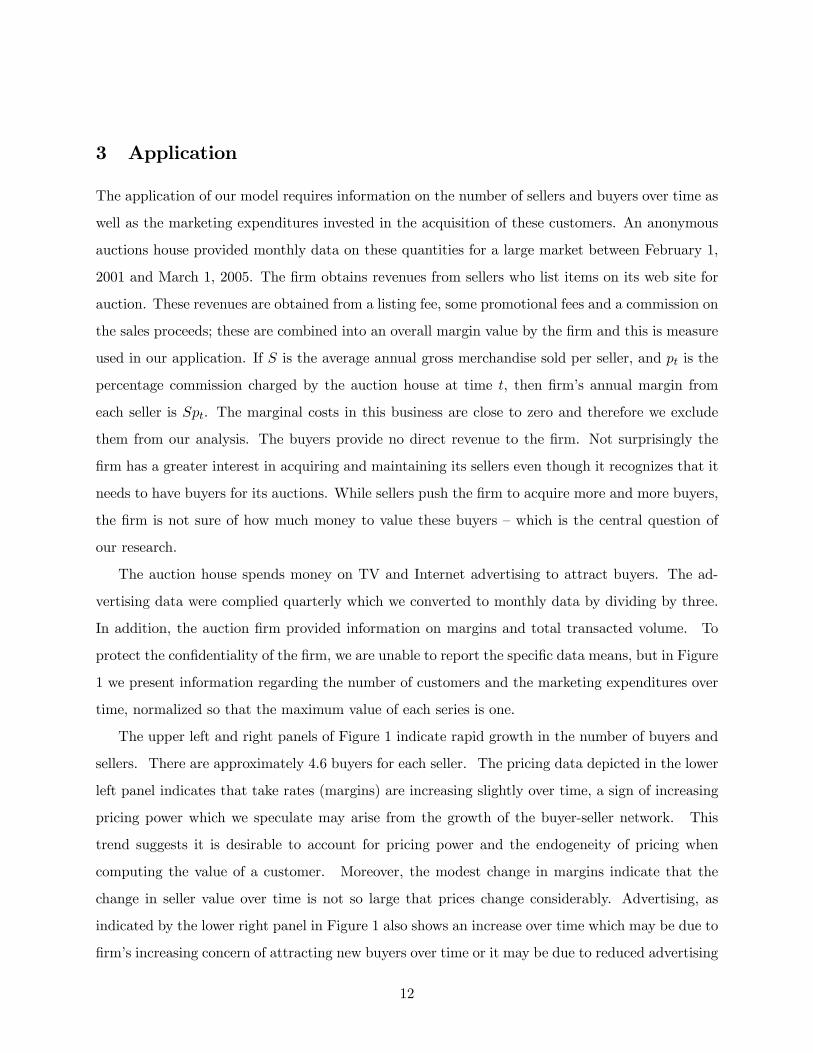
following figures depict the fit of the model to the data. In Figure 2 we present the model fit based
on a one-step ahead forecasts for period t based on (7) and (8), and the estimation residuals. In
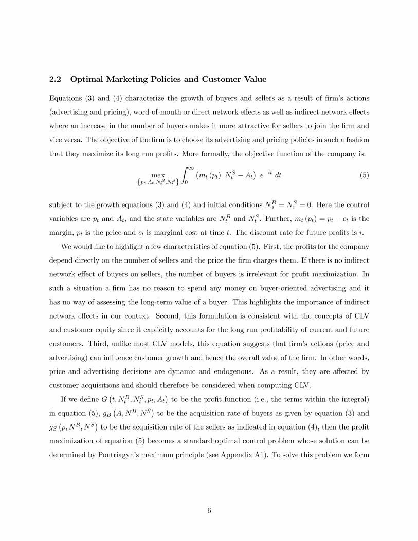
Figure 3, we use actual At, pt to generate a recursive forecast from period 0, and compare this
13
forecast with actual data. We conclude that the model provides a reasonably good fit to the data,
as indicated by Figure 3.5 The top panel of this figure provides one step ahead forecasts (using
data up to period t − 1 to forecast demand in t) and the lower panel is a recursive formula usingonly information at t = 0.
Figure 2: Model Fit and Residuals
4.2 Parameter Estimates
Table 1 presents the parameter estimates of our model along with the t-statistics.
5As the request of the sponsoring firm, the figure is normalized to disguise the data such that the maximumnumber of customers is scaled to one.
14
Figure 3: Recursive Forecast and Errors
Parameter Estimate t-statBuyers EquationIntercept x −0.004 −4.26Advertising h 0.0003 5.90Direct Network Effect of Buyers b −0.011 −2.45Indirect Network Effect of Sellers g 0.019 4.30Potential Market Size of Buyers (million) MB 50.72 13.29Sellers EquationIntercept φ −0.037 −2.90Price θ 0.015 2.96Direct Network Effect of Sellers β −0.066 −2.95Indirect Network Effect of Buyers γ 0.095 2.13Potential Market Size of Sellers (million) MS 7.50 4.29
Table 1: Parameter Estimates
All parameters are statistically significant. Advertising has a significantly positive impact on
the acquisition of buyers. Price has a significant negative impact on sellers growth (recall α(pt) =
15
φ− θ ln pt, so price parameter θ is expected to be positive). The parameters b and β are negative.
As discussed earlier, these parameter captures the net effect of word-of-mouth as well as customer
defection. The negative sign suggests that customer defection is outpacing the growth from word-of-
mouth effect. This defection may also be a result of "crowding" where customers prefer to list/buy
when fewer competitors are in the system.
The indirect network effects for both buyers and sellers are positive and very strong. This
suggests that the more buyers we have in the system the more sellers are attracted to the firm and
vice versa. Further, the indirect effect of buyers on sellers (0.095) is five times the indirect effect of
sellers on buyers (0.019). In other words, even though buyers do not provide any direct revenue to
the firm, they may be more critical for its growth. We will return to this issue when we translate
these into the value of buyers and sellers. In sum, in response to the first question we raised in the
introduction of this paper, we find that there are significant network effects present in our empirical
application.
The market potential for buyers is estimated to be about 50.7 million and the number of sellers
is estimated to be about 7.5 million. Though we can not reveal the specifics regarding the current
market size in order to protect the confidentiality of the firm, based on our market potential
estimates the market penetration of both populations is on the order of 1/5 the estimated market
potential. This indicates that there are significant growth opportunities for this firm that should
be reflected in its overall customer and firm value.
4.3 The Value of a Customer
In this section, we address the three pertinent managerial questions we asked in the beginning of
this paper.
1. What is the value of a buyer or a seller? In other words, what is the maximum the firm
should spend on acquiring a buyer or a seller. This estimate is especially difficult for buyers
who do not provide any direct revenue or profit to the firm.
2. How can the firm apportion the value of transactions between buyers and sellers?
3. How do these values change over time?
16
As indicated earlier, the value of a buyer is given by the Lagrangian multiplier of the optimal
control problem. In Appendix A4 we develop an analog in the discrete time context so we can apply
it to our data. In particular, we show that the shadow prices for buyers and sellers are given by
µλBt+1
λSt+1
¶= − (1 + i)−t
µ0
Spt
¶− (1 + i)−t
µD11t D12tD21t D22t
¶µ NSt S
(−θ(MS−NSt )/pt)
−1h(MB−NB
t )/At
¶. (19)
Using this equation and the model parameters we estimate the current value of a buyer as
approximately $550. Note that the entire value of buyers is derived from their indirect network
effect on the growth of sellers. Traditional models of CLV that do not account for these network
effects are unable to estimate the value of these "free" customers.
The value of a seller at the current time is about $500. Surprisingly the value of a seller is
slightly less than that of a buyer. This is counter-intuitive for at least two reasons. Although
the firm believes that buyers are important for its growth, its revenues are derived directly from
sellers. Therefore, intuitively it makes sense to assume that the paying customers or sellers are
more important for firm’s profits. The second reason that supports the firm’s intuition is the fact
that there are approximately 4.6 buyers for each seller. Since each transaction requires a buyer and
a seller, it is reasonable to argue that the value of a seller should be at least 4.6 times the value of
a buyer. Our model results go against this intuition and suggest that the value of a seller is almost
equal to or slightly less than the value of a buyer.
What explains this counter-intuitive result? First, Table 1 indicates that the parameter value
for the indirect network effect of buyers on sellers growth (0.095) is almost five times the parameter
value for the indirect network effect of sellers on buyers growth (0.019). Second, the net effect of
word-of-mouth and attrition on sellers is −0.066, suggesting a natural tendency to attrite. Third,as indicated by θ = 0.015, historical prices have had a negative impact on sellers’ growth. Fourth,
the negative intercept for seller’s equation (φ = −0.037) suggests that there is no "organic" or"natural" growth of the seller population. In other words, except for the indirect network effect
of buyers, all other factors are working against the growth of sellers. This makes the buyers even
more critical for the overall growth and profitability of the firm. In the end, even though the firm
has 4.6 buyers for each seller, the indirect network effect of a buyer is almost five times the indirect
network effect of a seller. The net result of all these factors is such that the value of a seller is
17
almost equal to (or slightly less than) the value of a buyer.
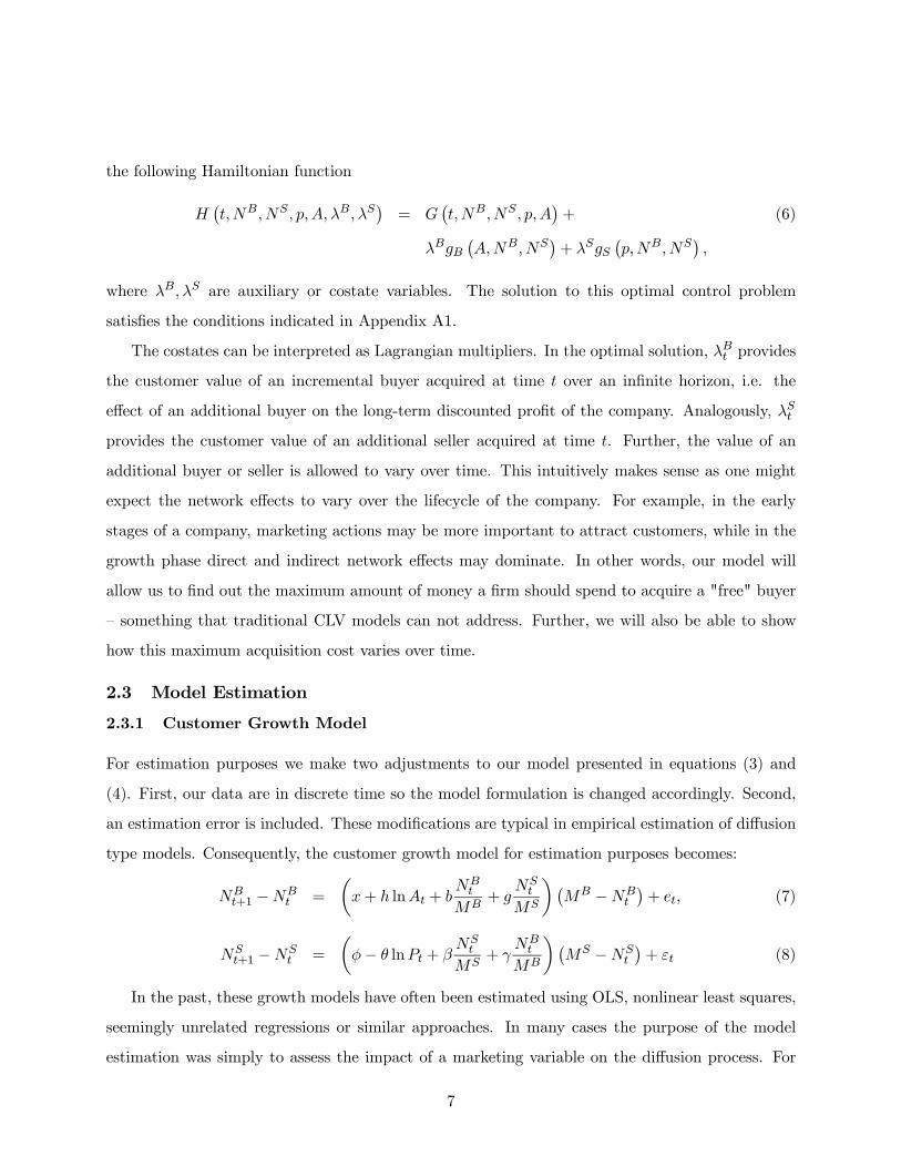
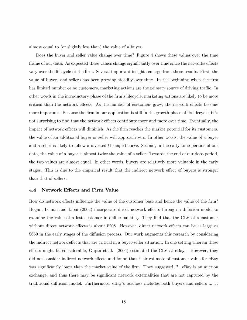
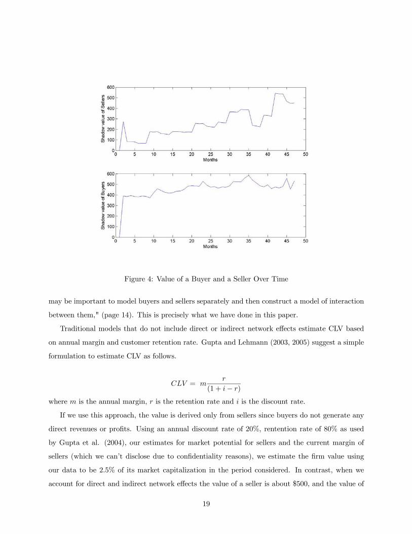
Does the buyer and seller value change over time? Figure 4 shows these values over the time
frame of our data. As expected these values change significantly over time since the networks effects
vary over the lifecycle of the firm. Several important insights emerge from these results. First, the
value of buyers and sellers has been growing steadily over time. In the beginning when the firm
has limited number or no customers, marketing actions are the primary source of driving traffic. In
other words in the introductory phase of the firm’s lifecycle, marketing actions are likely to be more
critical than the network effects. As the number of customers grow, the network effects become
more important. Because the firm in our application is still in the growth phase of its lifecycle, it is
not surprising to find that the network effects contribute more and more over time. Eventually, the
impact of network effects will diminish. As the firm reaches the market potential for its customers,
the value of an additional buyer or seller will approach zero. In other words, the value of a buyer
and a seller is likely to follow a inverted U-shaped curve. Second, in the early time periods of our
data, the value of a buyer is almost twice the value of a seller. Towards the end of our data period,
the two values are almost equal. In other words, buyers are relatively more valuable in the early
stages. This is due to the empirical result that the indirect network effect of buyers is stronger
than that of sellers.
4.4 Network Effects and Firm Value
How do network effects influence the value of the customer base and hence the value of the firm?
Hogan, Lemon and Libai (2003) incorporate direct network effects through a diffusion model to
examine the value of a lost customer in online banking. They find that the CLV of a customer
without direct network effects is about $208. However, direct network effects can be as large as
$650 in the early stages of the diffusion process. Our work augments this research by considering
the indirect network effects that are critical in a buyer-seller situation. In one setting wherein these
effects might be considerable, Gupta et al. (2004) estimated the CLV at eBay. However, they
did not consider indirect network effects and found that their estimate of customer value for eBay
was significantly lower than the market value of the firm. They suggested, "...eBay is an auction
exchange, and thus there may be significant network externalities that are not captured by the
traditional diffusion model. Furthermore, eBay’s business includes both buyers and sellers ... it
18
Figure 4: Value of a Buyer and a Seller Over Time
may be important to model buyers and sellers separately and then construct a model of interaction
between them," (page 14). This is precisely what we have done in this paper.
Traditional models that do not include direct or indirect network effects estimate CLV based
on annual margin and customer retention rate. Gupta and Lehmann (2003, 2005) suggest a simple
formulation to estimate CLV as follows.
CLV = mr
(1 + i− r)where m is the annual margin, r is the retention rate and i is the discount rate.
If we use this approach, the value is derived only from sellers since buyers do not generate any
direct revenues or profits. Using an annual discount rate of 20%, rentention rate of 80% as used
by Gupta et al. (2004), our estimates for market potential for sellers and the current margin of
sellers (which we can’t disclose due to confidentiality reasons), we estimate the firm value using
our data to be 2.5% of its market capitalization in the period considered. In contrast, when we
account for direct and indirect network effects the value of a seller is about $500, and the value of
19
a buyer is about $550. Given the estimated market potential of 7.5 million sellers and 50.7 million
buyers, a rough estimate of the customer value of this firm is $500*7.5+$550*50.7 = $31.7 billion,
which is closer to 80% of the market capitalization of this firm in the period considered.6 Given
these data are from only one geographic market of the firm (albeit the largest), this valuation
seems reasonable and far better than one afforded by the traditional CLV approach that ignores
network effects. Interestingly, buyers account for almost 90% of the total customer value. While
we acknowledge that these are very crude estimates of market value, nonetheless they show that
ignoring network effects can underestimate the firm value significantly.
4.5 Price and Advertising Elasticities
Given the presence of strong network effects, how do the effectiveness of marketing actions change
over time? To address this question, we estimate the price and advertising elasticities with respect
to customer growth. In our model, advertising influences the growth of buyers and price affects the
sellers’ growth. The derivative of these marketing actions with respect to the number of buyers or
sellers is given by the following equations.
∂
∂AtgB¡At, N
Bt , N
St , et
¢=
h
At
¡MB −NB
t
¢∂
∂ptgS¡pt,N
Bt , N
St , εt
¢= − θ
pt
¡MS −NS
t
¢These equations capture the contemporaneous effects of advertising and price on the growth of
buyers and sellers. Figure 5 shows the trajectory of the advertising and price elasticity over time.
Two interesting results emerge from this figure. First, both the advertising and the price
elasticities are decreasing over time. In other words, as firms acquire more customers over time,
network effects become increasingly important. This diminishes the impact of advertising and price
on customer growth. Second, even in the early time periods sellers’ price elasticities (-0.16) are
small compared to the average price elasticity of -1.6 found by Tellis (1988) or -1.4 found by Bijmolt
et al. (2004). This suggests that sellers have limited power given the auction house in the presence
of strong network effects. Third, the advertising elasticity for buyers is a maximum of 0.006 in6We recognize that for both approaches, strictly speaking, we should forecast the number of customers in the
future as well their future value in each time period and use appropriate discounting. While this is straightforwardin the traditional CLV model as shown by Gupta et al. (2004), it is a complex dynamic problem when direct andindirect network effects are included. We leave the exact solution for future research. Our purpose here is to get arough estimation to show the significant differences that arise when we account for network effects.
20
Figure 5: Advertising and Price Elasticity Over Time
the early periods and rapidly goes down over time. In a meta analysis, Lodish et al. (1995) found
that the ad elasticities range from 0.05 for established products to 0.26 for new products. The
low advertising elasticities in our application again suggest that in our application network effects
are more pronounced and effective in acquiring customers than traditional advertising. With the
changing landscape of advertising, the growth of new media and the explosion of viral marketing,
the advertising elasticities in our study may be more reflective of the current status and effectiveness
of advertising.
5 Conclusions
Customer profitability is a central consideration to many firms. Though research in this area is
burgeoning, little work to date addresses the issue of customer valuation in the context of direct and
indirect network effects in a dynamic setting. This limitation is palpable because network effects
exist in many contexts including sellers and buyers for auction houses, job seekers and job provides
on job sites, real estate listings and buyers on listing services, and so forth. In these contexts,
21
traditional methods of customer valuation that are based on summing an individual customer’s
cash flows are misleading, as the interaction of populations is relevant to customer valuation. Even
customers that provide no direct source of revenue add value to the firm. For example, a job
seeker does not pay for a job, but an increase in the number of job seekers makes a job listing more
valuable to an employer, and hence the listing agency. Therefore, CLV is not solely a function of
the cash flows generated by a customer, but also the effect this customer has on attracting other
customers. In addition extant methods of valuing customers do not consider the role that customer
acquisitions play in affecting marketing expenditures. This can also affect CLV, especially in the
presence of network effects, as firms can reduce their marketing expenses as network grows and the
diminution in costs further amplifies customer value.
We address these problems by offering a new approach to assess customer value that is predicated
upon the incremental profits to the firm over an infinite horizon as a result of adding another buyer
or seller to the firm’s portfolio of customers. To do this, we begin by developing a diffusion-type
model of the growth in the firm’s buyer and seller customer populations over time. In this model,
the size of each customer population is a function of a firm’s marketing, direct network effects,
and indirect network effects. We then use this system of growth equations, coupled with margin
data and marketing expenditures, to determine firm profits over time. The resulting first order
conditions for marketing spend over time imply an optimal price and advertising path. This leads
to four equations which we estimate via GMM: the seller growth model, the buyer growth model,
the advertising spend over time, and the pricing over time. Using the parameter estimates from this
model, it is possible to compute the Lagrange multipliers arising from the constraints that the seller
and buyer growth models place on a firms’ infinite horizon profits. The Lagrange multiplier for
buyers (providers) are a natural measure of the marginal impact of an additional buyer or seller on
a firms’ net discounted sum of future profits, and hence provide the CLV of each type of customer.
The presence of network effects led to a number of questions we set forth at the start of this
paper. We reprise these question here and our findings pertaining to each in the considered appli-
cation (and note that the method developed in this paper could afford answers to these questions
in other applications as well):
• Are direct and indirect network effects present in practice? We find strong evidence of the
presence of network effects, and find the network effects of buyers on seller are nearly six
22
times the effect of seller on buyers.
• How much should a company spend to acquire new customers in the presence of these networkeffects? In the considered context, we find that each type of customer provides the firm with
roughly $500-550 over the lifetime of the customer.
• How does the value of a customer change over time? The value of the customers is increasingover time as the network builds, and we expect the network to reach a point wherein an
additional customer no longer enhances the effect of the network.
• How do we apportion value between buyers and sellers? Though there exist 4.6 seller for each
buyer, we find each to have roughly equal value. This counterintuitive effect is explained in
part by the greater indirect network effect associate with buyers and a greater tendency of
seller to attrite.
• How should firms’ marketing efforts change over time in the presence of network effects?
How do customers’ sensitivities to these marketing actions change over time? As the network
effect become stronger, marketing plays less of a role in attracting buyers and sellers. Hence,
elasticities decrease as well as the optimal spend.
• Does the omission of network effects understate the value of customer base and hence thevalue of a firm? We find that traditional CLV methods capture only 2% of the firms’ value
whereas the approach indicated herein affords a good approximation of firm value.
Given the nascent state of customer valuation research in the context of network effects, there
remain many potential directions in which the foregoing analysis can be extended. First, as richer
data become available in more contexts, our analysis can be further generalized. One extension of
particular interest is to forecast future expenses, demand and customer value. This would require
the resolution of a stochastic dynamic program to solve the infinite horizon problem. In sum, we
hope this initial foray into customer valuation in the context of network effects leads to additional
insights that will be useful to firms who are concerned with managing their customer portfolio in
a networked economy.
23
References
[1] Ascher, U. M.; R. M. M. Mattheij; R. D. Russell (1995): Numerical Solution ofBoundary Value Problems for Ordinary Differential Equations. SIAM’s Classics in AppliedMathematics, 13, SIAM, Philadelphia.
[2] Bertsekas D. P. (1995): Dynamic programming and optimal control. Vols.1 and 2. AthenaScientific, Belmont, MA.
[3] Bijmolt, Tammo H.A., Harald J. Van Heerde, and Rik G.M. Pieters (2005), “NewEmpirical Generalizations on the Determinants of Price Elasticity,” Journal of Marketing Re-search, 42 (May), 141-156.
[4] Brock, W. A. and A. G. Malliaris (1989): Differential Equations, Stability and Chaos inDynamic Economics. North-Holland, Oxford.
[5] Chamberlain, Gary S. (1987), "Asymptotic Efficiency in Estimation with ConditionalMoment Restrictions," Journal of Econometrics, 34, 305-334.
[6] Chiang, A. C. (1992): Elements of Dynamic Optimization. McGraw Hill, New York.
[7] Chintagunta, Pradeep and Naufel Vilcassim (1992),"An Empirical Investigation ofAdvertising Strategies in a Dynamic Duopoly, " Management Science, 38 (9), 1230—1244.
[8] Chintagunta, Pradeep and Vithala Rao (1996),"Pricing Strategies in a DynamicDuopoly: A Differential Game Model, " Management Science, 42 (11), 1501—1514.
[9] Demange, Gabrielle and David Gale (1985), "The Strategy Structure of Two-SidedMatching Markets," Econometrica, 53, 4 (July), 873-888.
[10] Dockner, Engelbert and Steffen Jorgensen (1988), “Optimal Pricing Strategies forNew Products in Dynamic Oligopolies,” Marketing Science, 7 (4), 315-334.
[11] Feichtinger, Gustav, Richard Hartl and Suresh Sethi (1994),"Dynamic OptimalControl Models in Advertising: Recent Developments, " Management Science, 40 (2), 195-226.
[12] Gupta, Sachin, Dipak Jain and Mohanbir sawhney (1999), “Modeling the Evolution ofMarkets with Indirect Network Externalities: An Application to Digital Television,”MarketingScience, 18 (3), 396-416.
[13] Gupta, Sunil and Donald R. Lehmann (2003), ), “Customers as Assets,” Journal ofInteractive Marketing, 17(1), Winter, 9-24.
[14] Gupta, Sunil, Donald R. Lehmann and Jennifer Ames Stuart (2004), “Valuing Cus-tomers," Journal of Marketing Research„ 41(1), 7-18.
[15] Gupta, Sunil and Valarie Zeithaml (2006), “Customer Metrics and Their Impact onFinancial Performance,” Marketing Science, forthcoming.
24
[16] Hansen, Lars Peter (1982), "Large Sample Properties of Generalized Method of MomentsEstimators," Econometrica, 50, 4. (July), 1029-1054.
[17] Hogan, John, Katherine Lemon and Barak Libai (2003),“What is the True Value ofa Lost Customer?” Journal of Service Research, 5(3), February, 196-208.
[18] Horsky, Dan and Leonard S. Simon (1983), "Advertising and the Diffusion of New Prod-ucts," Marketing Science, 2, (1) (Winter, 1983), 1-17.
[19] Horsky, Dan and Karl Mate (1988), "Dynamic Advertising Strategies of CompetingDurable Good Producers," Marketing Science, 7 (4), 356-367.
[20] Kadiyali, Vrinda, Pradeep Chintagunta, and Nafuel Vilcassim (2000),"Manufacturer-Retailer Channel Interactions and Implications for Channel Power: An Em-pirical Investigation of Pricing in a Local Market," Marketing Science, 19, 2 (Spring), 127-148.
[21] Kalish, Shlomo (1985), "A New Product Adoption Model with Price, Advertising andUncertainty," Management Science, 31 (12), 1569—1585.
[22] Kamakura, Wagner A, Carl F. Mela, Asim Ansari, Anand Bodapati, Pete Fader,Raghuram Iyengar, Prasad Naik Scott Neslin, Baohong Sun, Peter Verhoef,Michel Wedel, and Ron Wilcox (2005), "Choice Models and Customer RelationshipManagement," Marketing Letters, 16, 3/4, 279-291.
[23] Katz, M. and C. Shapiro (1985), "Network externalities, competition, and compatibility",American Economic Review, 75 (3), 424-440.
[24] Katz, M. and C. Shapiro (1986), “Technology Adoption in the Presence of Network Exter-nalities”, Journal of Political Economy, 94, 22-41.
[25] Kumar, V. and Trichy Krishnan (2002),"Multinational Diffusion Models: An AlternativeFramework," Marketing Science, 21 (3), 318-330.
[26] Lions, J. L. (1971): Optimal Control of Systems Governed by Partial Differential Equations.Springer Verlag, New York.
[27] Lodish, Leonard M., Magid Abraham, Stuart Kalmenson, Jeanne Livelsberger,Beth Lubetkin, Bruce Richardson, and Mary Ellen Stevens (1995), “How T.V.Advertising Works: A Meta-Analysis of 389 Real World Split Cable T.V. Advertising Experi-ments,” Journal of Marketing Research, 32 (May), 125—139.
[28] Marketing Science Institute (2006), "2006-2008 Research Priorities," Research Report,Boston, Massachusetts.
[29] Neil, G., M. Kende and R. Rob (2000), "The dynamics of technological adoption in Hard-ware/software systems: the case of compact disc players," The RAND Journal of Economics,31 (1), 43-61.
25
[30] Newey, Whitney K. and Daniel. McFadden (1994), "Large Sample Estimation andHypothesis Testing," in Handbook of Econometrics, vol. iv, ed. by R. F. Engle and D. L.McFadden, pp. 2111-2245, Amsterdam: Elsevier.
[31] Newey, Whitney K. and Kenneth D. West (1987): "A Simple, Positive Semi-Definite,Heteroskedasticity and Autocorrelation Consistent Covariance Matrix," Econometrica, 55, 3.(May, 1987), 703-708.
[32] Pontryagin, L. S.; V. Boltyanskii; R. V. Gamkrelidze and E. F. Mishenko (1964):The mathematical theory of optimal processes. Mc Millan, New York.
[33] Reinartz, Werner and V. Kumar (2003), “The impact of customer relationship charac-teristics on profitable lifetime duration,” Journal of Marketing, 67(1), January, 77-99.
[34] Reinartz, Werner, Jacquelyn Thomas and V. Kumar (2005), “Balancing Acquisitionand Retention Resources to Maximize Customer Profitability,” Journal of Marketing, 69 (1),January, 63-79.
[35] Rust, Roland, Katherine Lemon and Valarie Zeithaml (2004), “Return on Mar-keting: Using Customer Equity to Focus Marketing Strategy,” Journal of Marketing, 68(1),January, 109-126.
[36] Seierstad, A. & Sydsaeter, K. (1987): Optimal Control Theory with Economic Applica-tions. Advanced Textbooks in Economics, (C. J. Bliss and M. D. Intriligator Editors ), Vol.24. North-Holland, New York.
[37] Simon, Hermann and Karl-Heinz Sebastian (1987),"Diffusion and Advertising: TheGerman Telephone Campaign, " Management Science, 33 (4), 451-466.
[38] Thompson, Gerald and Jinn-Tsair Teng (1984), "Optimal Pricing and AdvertisingPolicies for New Product Oligopoly Models," Marketing Science, 3 (2), 148-168.
[39] Venkatesan, Rajkumar and V. Kumar (2004),“A Customer Lifetime Value Frameworkfor Customer Selection and Resource Allocation Strategy,” Journal of Marketing, 68 (4), 106-125.
[40] Yao, Song and Carl F. Mela (2006), "Online Auction Demand," Working Paper, DukeUniversity.
26
Appendix
A1 Optimal Control Solution
Equation (6) gives the following Hamiltonian function
H¡t,NB, NS, p, A,λB,λS
¢= G
¡t,NB,NS , p, A
¢+λBgB
¡A,NB, NS
¢+λSgS
¡p,NB, NS
¢, (A-1)
where λB,λS are auxiliary or costate variables. The solution to this optimal control problem
satisfies the following conditions,
0 =∂
∂pH =
∂
∂pG¡t,NB
t ,NSt , pt, At
¢+ λSt
∂
∂pgS¡pt,N
Bt ,N
St
¢,
0 =∂
∂AH =
∂
∂AG¡t,NB
t , NSt , pt, At
¢+ λBt
∂
∂AgB¡At,N
Bt , N
St
¢,
·NB
t =∂
∂λBH = gB
¡At,N
Bt , N
St
¢,
·NS
t =∂
∂λSH = gS
¡pt, N
Bt , N
St
¢,
·λB
t = − ∂
∂NBH = − ∂
∂NBG¡t,NB
t , NSt , pt, At
¢− λSt∂
∂NBgS¡pt, N
Bt , N
St
¢−λBt
∂
∂NBgB¡At,N
Bt , N
St
¢,
·λS
t = − ∂
∂NBH = − ∂
∂NSG¡t,NB
t , NSt , pt, At
¢− λSt∂
∂NSgS¡pt, N
Bt , N
St
¢−λBt
∂
∂NSgB¡At,N
Bt ,N
St
¢,
together with the initial conditions NB0 = N
S0 = 0, and the transversality conditions
limT→∞
λBTNBT = 0, lim
T→∞λSTN
ST = 0,
(see e.g., Pontryagin et al. 1964, Lions 1971, Seierstad and Sydsaeter 1987, Chiang 1992 and
Bertsekas 1995).
27
A2 The Euler Equation
To solve the dynamic problem indicated by (9) we being by defining the optimal value function:
for an arbitrary initial point¡NS0 , N
B0 , e0, ε0
¢this function is given by:
V¡NS0 , N
B0 , e0, ε0
¢= maxpt,At
E0
" ∞Xt=0
δtG¡NBt , N
St , pt, At
¢#. (A-2)
Then, the Jacobi-Bellman condition states that the solution satisfies the following recursion for
Therefore, the first order conditions associated to the right hand side optimization problem are
satisfied, which are
∂
∂ptG¡NBt ,N
St , pt, At
¢+ δEt
"∂
∂NSt+1
V¡NBt+1, N
St+1, et+1, εt+1
¢# ∂
∂ptgS¡pt, N
Bt , N
St , εt
¢= 0,(A-4)
∂
∂AtG¡NBt , N
St , pt, At
¢+ δEt
"∂
∂NBt+1
V¡NBt+1,N
St+1, et+1, εt+1
¢# ∂
∂AtgB¡At, N
Bt , N
St , et
¢= 0.(A-5)
Using the envelope theorem, it can be proved that
µ ∂∂NB
tV¡NBt , N
St , et, εt
¢∂
∂NStV¡NBt ,N
St , et, εt
¢¶ = µ ∂∂NB
tG¡NBt ,N
St , pt, At
¢∂
∂NStG¡NBt , N
St , pt, At
¢¶+ δ
×Ã
∂∂NB
tgB¡pt, N
Bt , N
St , εt
¢∂
∂NBtgS¡At,N
Bt ,N
St , et
¢∂
∂NStgB¡pt, N
Bt , N
St , εt
¢∂
∂NStgS¡At, N
Bt , N
St , et
¢ !Et⎡⎣µ ∂
∂NBt+1V¡NBt+1, N
St+1, et+1, εt+1
¢∂
∂NSt+1V¡NBt+1, N
St+1, et+1, εt+1
¢¶⎤⎦(A-6)
28
Sustituting Eth
∂∂NB
t+1V¡NBt+1,N
St+1, et+1, εt+1
¢iand Et
h∂
∂NSt+1V¡NBt+1,N
St+1, et+1, εt+1
¢ifrom
(A-4) and (A-5) into (A-6),
µ ∂∂NB
tV¡NBt , N
St , et, εt
¢∂
∂NStV¡NBt , N
St , et, εt
¢¶ = µ ∂∂NB
tG¡NBt , N
St , pt, At
¢∂
∂NStG¡NBt , N
St , pt, At
¢
+
̶
∂NBtgB¡pt,N
Bt ,N
St , εt
¢∂
∂NBtgS¡At, N
Bt , N
St , et
¢∂
∂NStgB¡pt, N
Bt , N
St , εt
¢∂
∂NStgS¡At,N
Bt , N
St , et
¢ !µ ∂G(NBt ,N
St ,pt,At)/∂pt
∂gS(pt,NBt ,N
St ,εt)/∂pt
∂G(NBt ,N
St ,pt,At)/∂At
∂gB(At,NBt ,N
St ,et)/∂At
¶(A-7)
updating the resulting condition and combining it with the first order conditions (A-4), (A-5) yields
the system,
µ ∂G(NBt ,N
St ,pt,At)/∂pt
∂gS(pt,NBt ,N
St ,εt)/∂pt
∂G(NBt ,N
St ,pt,At)/∂At
∂gB(At,NBt ,N
St ,et)/∂At
¶= δ Et
⎡⎣µ ∂∂NB
t+1G¡NBt+1,N
St+1, pt+1, At+1
¢∂
∂NSt+1G¡NBt+1,N
St+1, pt+1, At+1
¢
+
à ∂∂NB
t+1gB¡pt+1,N
Bt+1, N
St+1, εt+1
¢∂
∂NBt+1gS¡At+1,N
Bt+1, N
St+1, et+1
¢∂
∂NSt+1gB¡pt+1,N
Bt+1, N
St+1, εt+1
¢∂
∂NSt+1gS¡At+1,N
Bt+1, N
St+1, et+1
¢ !
·µ ∂G(NB
t+1,NSt+1,pt+1,At+1)/∂pt+1
∂gS(pt+1,NBt+1,N
St+1,εt+1)/∂pt+1
∂G(NBt+1,N
St+1,pt+1,At+1)/∂At+1
∂gB(At+1,NBt+1,N
St+1,et+1)/∂At+1
¶⎤⎥⎦
This expression is the Euler equations system. Note that the left hand side can be introduced
in the conditional expectation with a sign change. Computing the partial derivatives, we obtain
the expression (14).
Et
⎡⎢⎣µ NSt S
θ(MS−NSt )/pt
1h(MB−NB
t )/At
¶+ (1 + i)−1
⎛⎜⎝µ 0
Spt+1
¶+
µD11t+1 D12t+1D21t+1 D22t+1
¶µ NSt+1S
(−θ(MS−NSt+1)/pt+1)
−1h(MB−NB
t+1)/At+1
¶⎞⎟⎠⎤⎥⎦ = 0,
29
where
D11t+1 = 1 +
µb
MB
¶¡MB −NB
t+1
¢−Ãx+ h lnAt+1 + bNBt+1
MB+ g
NSt+1
MS
!
= 1 + b− x− h lnAt+1 − 2bNBt+1
MB− gN
St+1
MS
D12t+1 =γ
MB
¡MS −NS
t+1
¢D21t+1 =
g
MS
¡MB −NB
t+1
¢D22t+1 = 1 +
β
MS
¡MS −NS
t+1
¢−Ãφ− θ lnPt+1 + βNSt+1
MS+ γ
NBt+1
MB
!− ρ
= 1 + β − φ+ θ ln pt+1 − 2βNSt+1
MS− γ
NBt+1
MB
A3 GMM Estimation
Equations (16), (17) and (18) yield a set of moment conditions. To simplify the notation, we
express these moment equations as E [m (Wt,Ω)] = 0, where Ω denotes the set of all parameters.
If this system of equations is just identified then one can use the method of moments. When the
system is overidentified as a result of adding more instrument conditions, then generalized method
of moments or GMM is used. In this approach we estimate the parameter vector by minimizing
the sum of squares of the differences between the population moments and the sample moments,
using the variance of the moments as a metric. Specifically, GMM estimates Ω by minimizing
QW (Ω) =
Ã1
T
TXt=1
m (Wt,Ω)
!0W−1
Ã1
T
TXt=1
m (Wt,Ω)
!, (A-8)
where W is a positive definite weight matrix. While the researcher cannot make the moment
conditions exactly equal to zero, s/he can choose parameters such that (A-8) is close to zero. The
choice of W impacts what it means to be close and the variance of the estimate bΩ depends onthis chosen matrix. It is always possible to choose W = I. However, this will, in general, lead to
inefficient estimates. The optimal W weights the moment conditions such that those conditions
with a high degree of variance get weighted less, thus affecting the minimization routine less. The
30
estimate bΩ with minimum variance is obtained for the limit variance covariance matrix,
WΩ0 = limT→∞
T ·E⎡⎣Ã 1
T
TXt=1
m (Wt,Ω0)
!Ã1
T
TXt=1
m (Wt,Ω0)
!0⎤⎦ (A-9)
=∞X
t=−∞E£m (W0,Ω0)m (Wt,Ω0)
0¤ ,i.e., WΩ0 is 2π times the spectral density matrix for m (Wt, θ0) at frequency zero. This matrixdepends on Ω0, and therefore the optimal GMM is unfeasible.
A feasible estimation is typically achieved using a two-step process. In the initial step, indicated
(0), a positive definite matrix W (0) matrix is chosen (e.g. W (0) = I, the identity matrix), leading
to a consistent initial set of parameter estimates bΩ(0). In the second step, we take the estimatebΩ(0) and estimate the variance-covariance estimator using the Barlett spectral density estimator ofWΩ0 ,
cWΩ0 = C0 +LXl=1
µ1− l
L
¶¡Cl +C
0l
¢, (A-10)
Cl = T−1T−lXt=1
m³Wt, bΩ(0)´m³Wt+l, bΩ(0)´0 = C 0−l,
as suggested by Newey and West (1987). A moderate number of lags L < T−1 is usually considered,thus L increases slowly with the sample size, so that T/L → ∞. This new weight matrix is thenused to solve the problem (A-8), and the resulting estimation bΩ(1) is an asymptotically efficientestimator of the true parameters. One can iterate over the weighting matrix M times (it does not
affect the asymptotic distribution, but the accuracy for small samples usually increases), but the
process converges sufficiently fast (e.g., in our context M < 5).
It has also been shown that, for the optimal weight,√T³bΩ− Ω´ is asymptotically distributed
N³0,¡Γ0W−1
Ω Γ¢−1´
with Γ = E£
∂∂Ω0m (Wt,Ω0)
¤, which can be estimated by Γ = T−1
PTt=1
Ω∂Ω0m (Wt,Ω0) .
In addition, T · QW
³bΩ´ is asymptotically distributed χ2r−k, where r is the number of equations
and k the number of parameters, and this can be used to test the overidentifying restrictions (see,
31
e.g., Hansen 1982, Chamberlain 1987 and Newey and McFadden 1994) to test the appropriateness
of the instruments.
The estimation is computed in two steps. In the first step, a Newey-West matrix was evaluated
at the starting values with L = 12, and in the second iteration we use Newey-West on the consistent
first step estimator.
A4 Lagrange Multipliers
We begin by characterising the solution to company problem via the Lagrange functional (11), for
each t ≥ 0,
∂E0
hX∞s=t
δsG¡NBs , N
Ss , ps, As
¢i∂pt
+ λSt+1∂gS
¡pt, N
Bt , N
St , εt
¢∂pt
= 0,
∂E0
hX∞s=t
δsG¡NBs , N
Ss , ps, As
¢i∂At
+ λBt+1∂gB
¡At, N
Bt , N
St , et
¢∂At
= 0,
∂E0
hX∞s=t
δsG¡NBs , N
Ss , ps, As
¢i∂NB
t
+ λBt − λBt+1∂gB
¡At, N
Bt , N
St , et
¢∂NB
t
−λSt+1∂gS
¡pt, N
Bt , N
St , εt
¢∂NB
t
= 0,
∂E0
hX∞s=t
δsG¡NBs , N
Ss , ps, As
¢i∂NS
t
− λBt+1∂gB
¡At, N
Bt , N
St , et
¢∂NS
t
+ λSt
−λSt+1∂gS
¡pt, N
Bt , N
St , εt
¢∂NS
t
= 0.
In the optimum E0
hX∞s=t
δ(s−t)G¡NBs , N
Ss , ps, As
¢i= V
¡NSt , N
Bt , et, εt
¢, therefore
E0
" ∞Xs=t
δsG¡NBs , N
Ss , ps, As
¢#= δt V
¡NSt , N
Bt , et, εt
¢,
32
and the first order conditions for each time t are,
δt∂
∂ptV¡NBt , N
St , et, εt
¢+ λSt+1
∂gS¡pt, N
Bt , N
St , εt
¢∂pt
= 0,
δt∂
∂AtV¡NBt , N
St , et, εt
¢+ λBt+1
∂gB¡At, N
Bt , N
St , et
¢∂At
= 0,
δt∂
∂NBt
V¡NBt , N
St , et, εt
¢+ λBt − λBt+1
∂gB¡At, N
Bt , N
St , et
¢∂NB
t
− λSt+1∂gS
¡pt, N
Bt , N
St , εt
¢∂NB
t
= 0,
δt∂
∂NSt
V¡NBt , N
St , et, εt
¢− λBt+1∂gB
¡At, N
Bt , N
St , et
¢∂NS
t
+ λSt − λSt+1∂gS
¡pt,N
Bt ,N
St , εt
¢∂NS
t
= 0.
Therefore,
λBt+1 = −δt∂
∂AtV¡NBt , N
St , et, εt
¢∂
∂AtgB¡At, NB
t , NSt , et
¢ ,λSt+1 = −δt
∂∂ptV¡NBt , N
St , et, εt
¢∂∂ptgS¡pt,NB
t ,NSt , εt
¢ ,also,
λBt = λBt+1∂gB
¡At, N
Bt , N
St , et
¢∂NB
t
+ λSt+1∂gS
¡pt, N
Bt , N
St , εt
¢∂NB
t
− δt∂V
¡NBt , N
St , et, εt
¢∂NB
t
,
λSt = λBt+1∂gB
¡At, N
Bt , N
St , et
¢∂NS
t
+ λSt+1∂gS
¡pt, N
Bt , N
St , εt
¢∂NS
t
− δt∂V
¡NBt , N
St , et, εt
¢∂NS
t
.
Note that last two equations can be used to compute the multipliers backwards, recursively
from the terminal transversality conditions. But in this paper we will use the two non-recursive
33
expressions for the Lagrange Multipliers,
λBt+1 = −δt∂
∂AtV¡NBt , N
St , et, εt
¢∂
∂AtgB¡At, NB
t , NSt , et
¢ = −δt ∂∂AtV¡gB¡At, N
Bt , N
St , et
¢, gS
¡pt, N
Bt , N
St , εt
¢, et+1, εt+1
¢∂
∂AtgB¡At,NB
t , NSt , et
¢= −δt ∂
∂NBt+1
V¡NBt+1,N
St+1, et+1, εt+1
¢.
λSt+1 = −δt∂∂ptV¡NBt , N
St , et, εt
¢∂∂ptgS¡pt,NB
t ,NSt , εt
¢ = −δt ∂∂ptV¡gB¡At,N
Bt ,N
St , et
¢, gS
¡pt, N
Bt , N
St , εt
¢, et+1, εt+1
¢∂∂ptgS¡pt, NB
t , NSt , εt
¢= −δt ∂
∂NSt+1
V¡NBt+1,N
St+1, et+1, εt+1
¢,
Using (A-7), we obtain that,
µλBt+1
λSt+1
¶= −δt
µ ∂∂NB
tV¡NBt ,N
St , et, εt
¢∂
∂NStV¡NBt , N
St , et, εt
¢¶ = −δtµ ∂∂NB
tG¡NBt , N
St , pt, At
¢∂
∂NStG¡NBt ,N
St , pt, At
¢
−δtÃ
∂∂NB
tgB¡pt, N
Bt , N
St , εt
¢∂
∂NBtgS¡At, N
Bt , N
St , et
¢∂
∂NStgB¡pt,N
Bt , N
St , εt
¢∂
∂NStgS¡At, N
Bt , N
St , et
¢ !µ ∂G(NBt ,N
St ,pt,At)/∂pt
∂gS(pt,NBt ,N
St ,εt)/∂pt
∂G(NBt ,N
St ,pt,At)/∂At
∂gB(At,NBt ,N
St ,et)/∂At
¶.
Computing the partial derivatives, we obtain the expression (19),