The Value of Distributed Solar Electric Generation to New Jersey and Pennsylvania

TheValueofDistributedSolarElectricGenerationtoNewJerseyandPennsylvania

Richard Perez

Benjamin L. Norris

Thomas E. Hoff

November 2012

Prepared for:

Mid‐Atlantic Solar Energy Industries Association

&

Pennsylvania Solar Energy Industries Association

Prepared by:

Clean Power Research

1700 Soscol Ave., Suite 22

Napa, CA 94559

Acknowledgements

This report was funded by the following organizations:

• The Reinvestment Fund’s Sustainable Development Fund

• Mid Atlantic Solar Energy Industries Association

• Advanced Solar Products

• SMA Americas

• Vote Solar

• Renewable Power

• Geoscape Solar

The authors wish to express their gratitude to Rachel Hoff for collecting and analyzing FERC filings from

the six utilities, producing the PV fleet simulations, and conducting the peak load day analysis; also to

Phil Gruenhagen for researching and preparing the PJM load and pricing data.

1

ExecutiveSummary

This report presents an analysis of value provided by grid‐connected, distributed PV in Pennsylvania and

New Jersey. The analysis does not provide policy recommendations except to suggest that each benefit

must be understood from the perspective of the beneficiary (utility, ratepayer, or taxpayer).

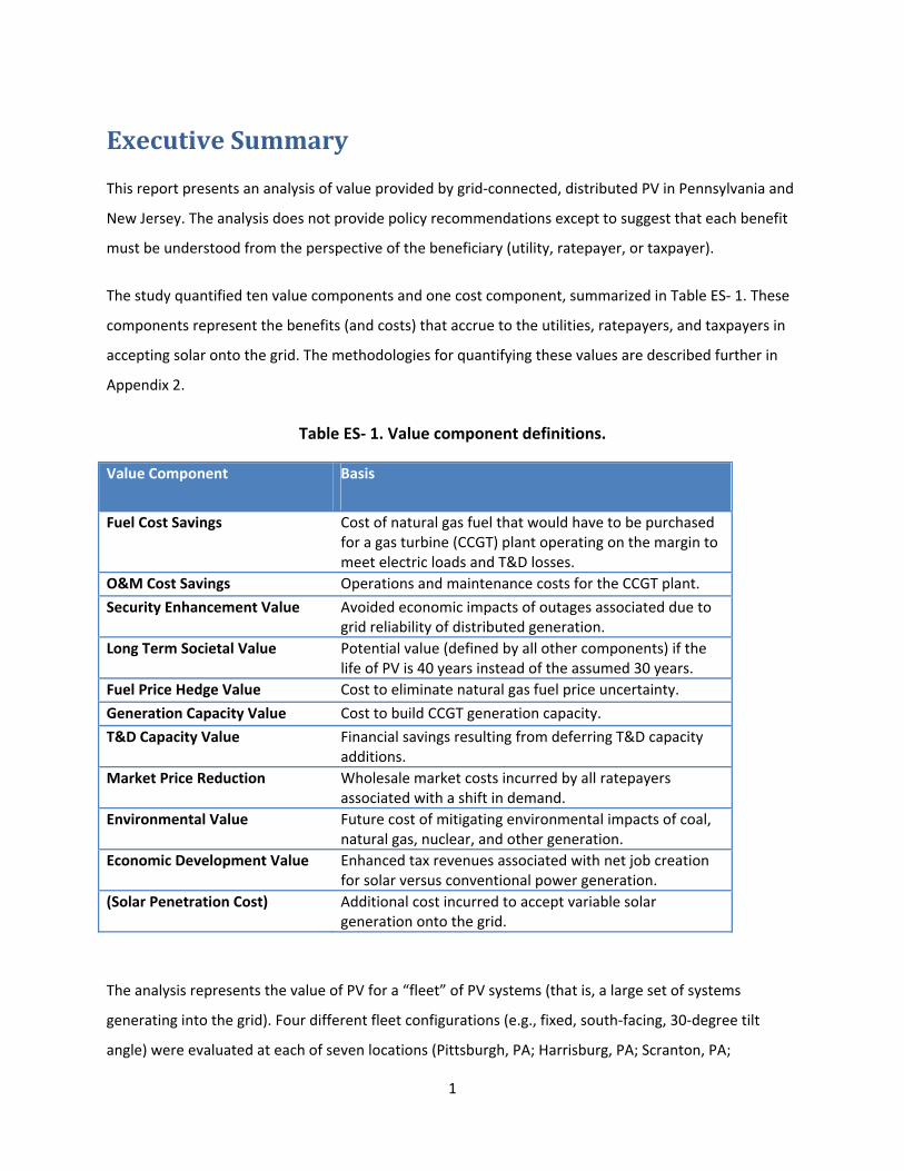
The study quantified ten value components and one cost component, summarized in Table ES‐ 1. These

components represent the benefits (and costs) that accrue to the utilities, ratepayers, and taxpayers in

accepting solar onto the grid. The methodologies for quantifying these values are described further in

Appendix 2.

Table ES‐ 1. Value component definitions.

Value Component Basis

Fuel Cost Savings Cost of natural gas fuel that would have to be purchased for a gas turbine (CCGT) plant operating on the margin to meet electric loads and T&D losses.

O&M Cost Savings Operations and maintenance costs for the CCGT plant.

Security Enhancement Value Avoided economic impacts of outages associated due to grid reliability of distributed generation.

Long Term Societal Value Potential value (defined by all other components) if the life of PV is 40 years instead of the assumed 30 years.

Fuel Price Hedge Value Cost to eliminate natural gas fuel price uncertainty.

Generation Capacity Value Cost to build CCGT generation capacity.

T&D Capacity Value Financial savings resulting from deferring T&D capacity additions.

Market Price Reduction Wholesale market costs incurred by all ratepayers associated with a shift in demand.

Environmental Value Future cost of mitigating environmental impacts of coal, natural gas, nuclear, and other generation.

Economic Development Value Enhanced tax revenues associated with net job creation for solar versus conventional power generation.

(Solar Penetration Cost) Additional cost incurred to accept variable solar generation onto the grid.

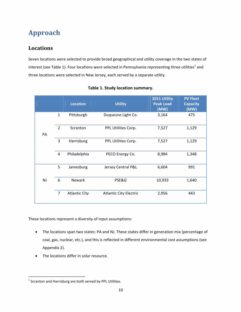
The analysis represents the value of PV for a “fleet” of PV systems (that is, a large set of systems

generating into the grid). Four different fleet configurations (e.g., fixed, south‐facing, 30‐degree tilt

angle) were evaluated at each of seven locations (Pittsburgh, PA; Harrisburg, PA; Scranton, PA;

2

Philadelphia, PA; Jamesburg, NJ; Newark, NJ; and Atlantic City, NJ). These locations represent a diversity

of geographic and economic assumptions across six utility service territories (Duquesne Light Co., PPL

Utilities Corp, PECO Utilities Corp, Jersey Central P&L, PSE&G, and Atlantic Electric).

The analysis represented a moderate assumption of penetration: PV was to provide 15% of peak electric

load for each study location (higher penetration levels result in lower value per MWh). PV was modeled

using SolarAnywhere®, a solar resource data set that provides time‐ and location‐correlated PV output

with loads. Load data and market pricing was taken from PJM for the six zones, and utility economic

inputs were derived from FERC submittals. Additional input data was taken from the EIA and the Bureau

of Labor Statistics (producer price indices).

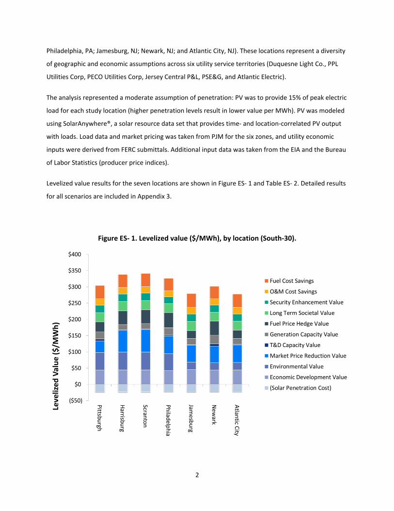
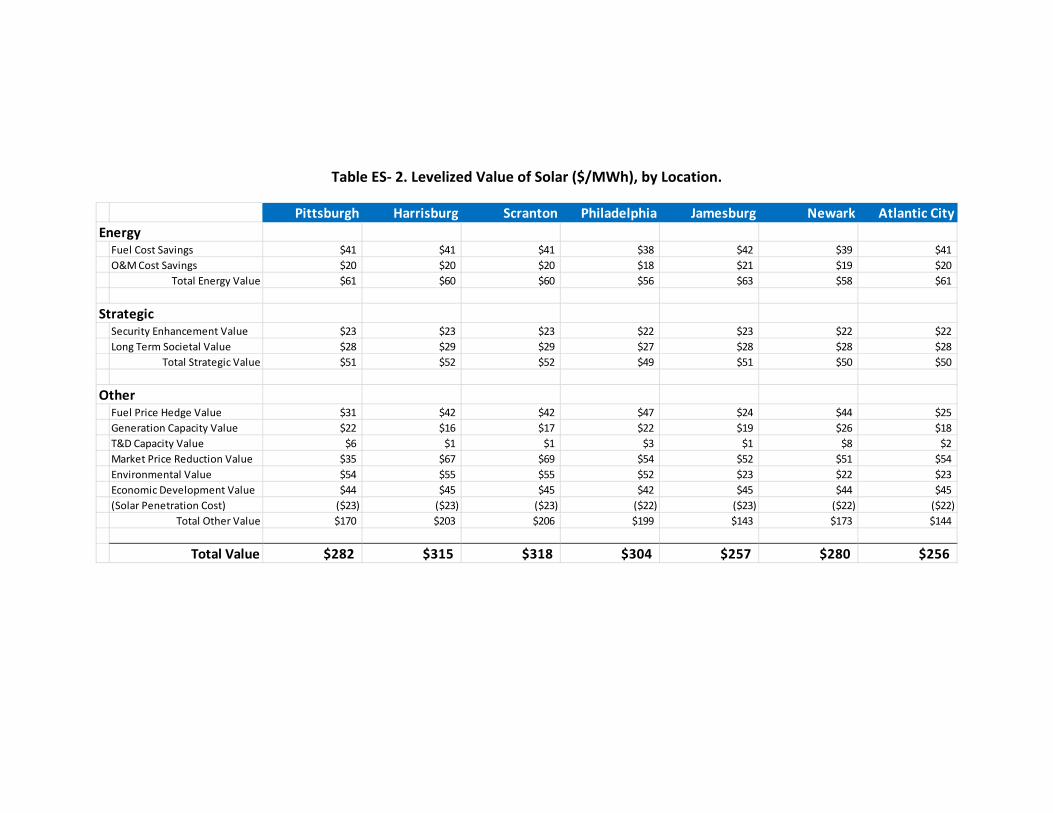
Levelized value results for the seven locations are shown in Figure ES‐ 1 and Table ES‐ 2. Detailed results

for all scenarios are included in Appendix 3.

Figure ES‐ 1. Levelized value ($/MWh), by location (South‐30).

3

The following observations and conclusions may be made:

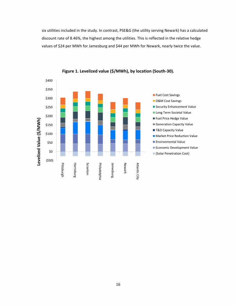
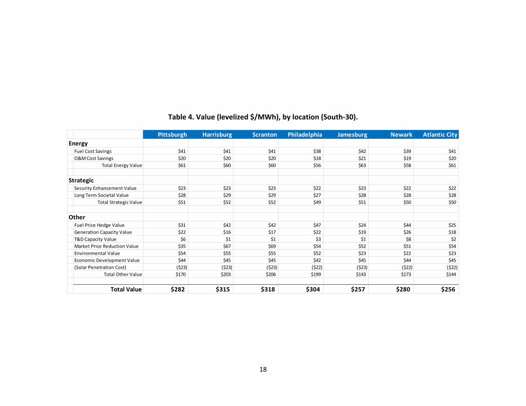
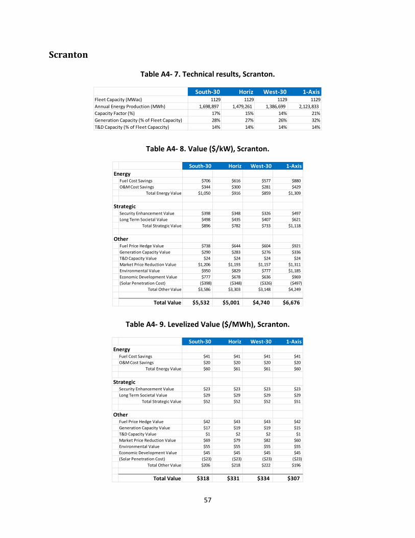
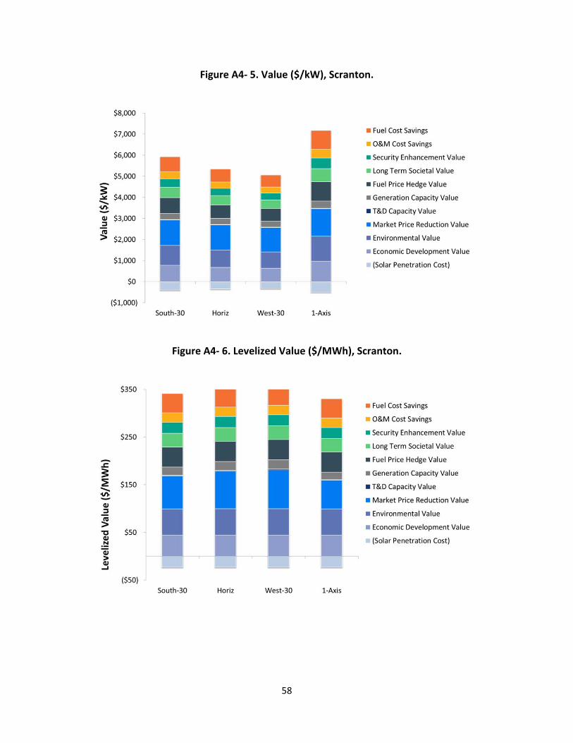
Total Value. The total value ranges from $256 per MWh to $318 per MWh. Of this, the highest

value components are the Market Price Reduction (averaging $55 per MWh) and the Economic

Development Value (averaging $44 per MWh).

Market Price Reduction. The two locations of highest total value (Harrisburg and Scranton) are

noted for their high Market Price Reduction value. This may be the result of a good match

between LMP and PV output. By reducing demand during the high priced hours, a cost savings is

realized by all consumers. Further investigation of the methods may be warranted in light of two

arguments put forth by Felder [32]: that the methodology does address induced increase in

demand due to price reductions, and that it only addresses short‐run effects (ignoring the

impact on capacity markets).

Environmental Value. The state energy mix is a differentiator of environmental value.

Pennsylvania (with a large component of coal‐fired generation in its mix) leads to higher

environmental value in locations in that state relative to New Jersey.

T&D Capacity Value. T&D capacity value is low for all scenarios, with the average value of only

$3 per MWh. This may be explained by the conservative method taken for calculating the

effective T&D capacity.

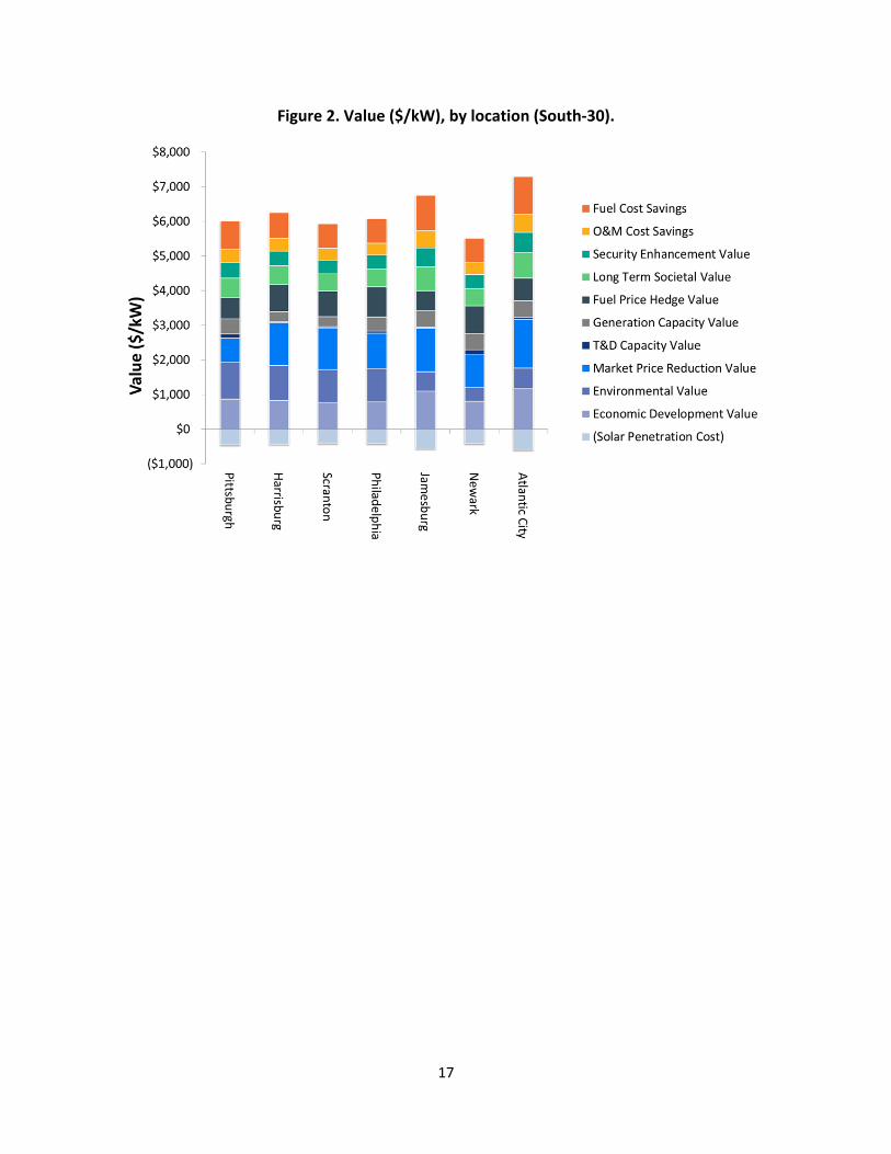
Fuel Price Hedge. The cost of eliminating future fuel purchases—through the use of financial

hedging instruments—is directly related to the utility’s cost of capital. This may be seen by

comparing the hedge value in Jamesburg and Atlantic City. At a utility discount rate of 5.68%,

Jersey Central Power & Light (the utility serving Jamesburg) has the lowest calculated cost of

capital among the six utilities included in the study. In contrast, PSE&G (the utility serving

Newark) has a calculated discount rate of 8.46%, the highest among the utilities. This is reflected

in the relative hedge values of $24 per MWh for Jamesburg and $44 per MWh for Newark,

nearly twice the value.

Generation Capacity Value. There is a moderate match between PV output and utility system

load. The effective capacity ranges from 28% to 45% of rated output, and this is in line with the

assigned PJM value of 38% for solar resources.

Table ES‐ 2. Levelized Value of Solar ($/MWh), by Location.

Pittsburgh Harrisburg Scranton Philadelphia Jamesburg Newark Atlantic City

EnergyFuel Cost Savings $41 $41 $41 $38 $42 $39 $41

O&M Cost Savings $20 $20 $20 $18 $21 $19 $20

Total Energy Value $61 $60 $60 $56 $63 $58 $61

StrategicSecurity Enhancement Value $23 $23 $23 $22 $23 $22 $22

Long Term Societal Value $28 $29 $29 $27 $28 $28 $28

Total Strategic Value $51 $52 $52 $49 $51 $50 $50

OtherFuel Price Hedge Value $31 $42 $42 $47 $24 $44 $25

Generation Capacity Value $22 $16 $17 $22 $19 $26 $18

T&D Capacity Value $6 $1 $1 $3 $1 $8 $2

Market Price Reduction Value $35 $67 $69 $54 $52 $51 $54

Environmental Value $54 $55 $55 $52 $23 $22 $23

Economic Development Value $44 $45 $45 $42 $45 $44 $45

(Solar Penetration Cost) ($23) ($23) ($23) ($22) ($23) ($22) ($22)

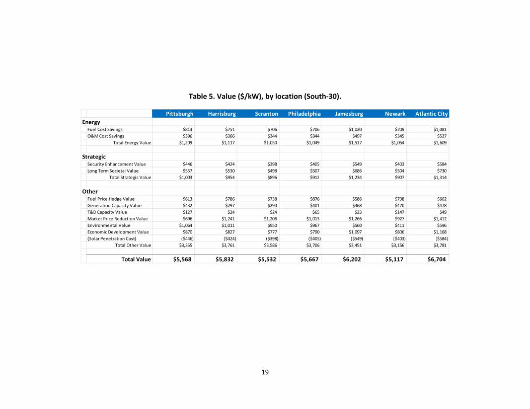
Total Other Value $170 $203 $206 $199 $143 $173 $144

Total Value $282 $315 $318 $304 $257 $280 $256

5

ContentsAcknowledgements ....................................................................................................................................... ii

Executive Summary ....................................................................................................................................... 1

Introduction: The Value of PV ....................................................................................................................... 7

Fuel Cost Savings ....................................................................................................................................... 7

O&M Cost Savings ..................................................................................................................................... 7

Security Enhancement Value .................................................................................................................... 8

Long Term Societal Value .......................................................................................................................... 8

Fuel Price Hedge Value ............................................................................................................................. 8

Generation Capacity Value ....................................................................................................................... 8

T&D Capacity Value ................................................................................................................................... 8

Market Price Reduction ............................................................................................................................ 9

Environmental Value ................................................................................................................................. 9

Economic Development Value .................................................................................................................. 9

Solar Penetration Cost .............................................................................................................................. 9

Value Perspective ...................................................................................................................................... 9

Approach ..................................................................................................................................................... 10

Locations ................................................................................................................................................. 10

Penetration Level .................................................................................................................................... 11

Fleet Configurations ................................................................................................................................ 11

Scenarios and Fleet Modeling ................................................................................................................. 12

Results ......................................................................................................................................................... 13

Utility Analysis ......................................................................................................................................... 13

PV Technical Analysis .............................................................................................................................. 13

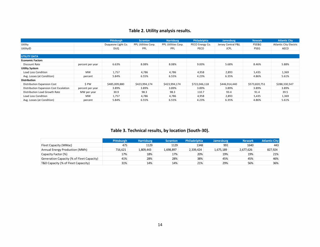
Value Analysis ......................................................................................................................................... 15

6

Future Work ................................................................................................................................................ 20

Appendix 1: Detailed Assumptions ............................................................................................................. 21

Appendix 2: Methodologies ........................................................................................................................ 23

Overview ................................................................................................................................................. 23

Units of Results ....................................................................................................................................... 23

PV Production and Loss Savings .............................................................................................................. 24

Loss Savings ............................................................................................................................................. 26

Fuel Cost Savings and O&M Cost Savings ............................................................................................... 28

Security Enhancement Value .................................................................................................................. 29

Long Term Societal Value ........................................................................................................................ 30

Fuel Price Hedge Value ........................................................................................................................... 31

Generation Capacity Value ..................................................................................................................... 32

T&D Capacity Value ................................................................................................................................. 33

Market Price Reduction Value ................................................................................................................ 33

Environmental Value ............................................................................................................................... 43

Economic Development Value ................................................................................................................ 45

Solar Penetration Cost ............................................................................................................................ 47

Methodology References ........................................................................................................................ 48

Appendix 3: Detailed Results ...................................................................................................................... 51

Pittsburgh ................................................................................................................................................ 52

Harrisburg ............................................................................................................................................... 54

Scranton .................................................................................................................................................. 57

Philadelphia ............................................................................................................................................. 59

Jamesburg ............................................................................................................................................... 61

Newark .................................................................................................................................................... 63

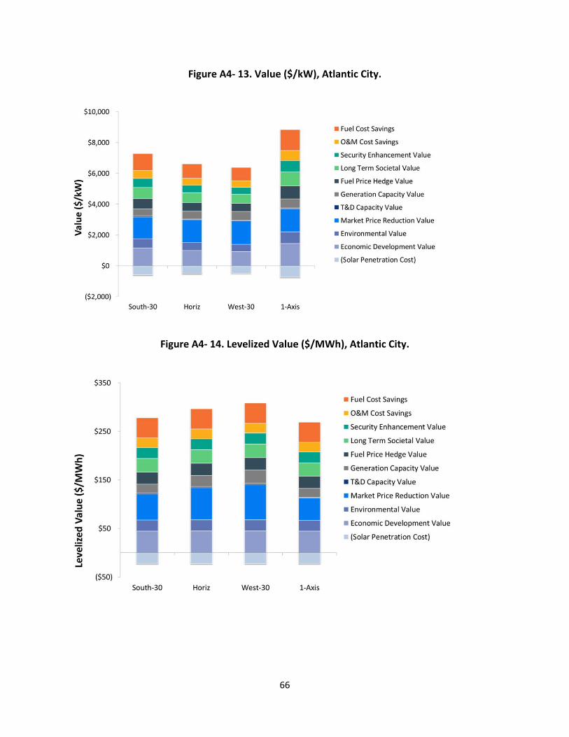
Atlantic City ............................................................................................................................................. 65

7

Introduction:TheValueofPV

This report attempts to quantify the value of distributed solar electricity in Pennsylvania and New

Jersey. It uses methodologies and analytical tools that have been developed over several years. The

framework supposes that PV is located in the distribution system. PV that is located close to the loads

provides the highest value per unit of energy to the utility because line losses are avoided, thereby

increasing the value of solar relative to centrally‐located resources.

The value of PV may be considered the aggregate of several components, each estimated separately,

described below. The methods used to calculate value are described in more detail in the Appendices.

FuelCostSavings

Distributed PV generation offsets the cost of power generation. Each kWh generated by PV results in

one less unit of energy that the utility needs to purchase or generate. In addition, distributed PV reduces

system losses so that the cost of the wholesale generation that would have been lost must also be

considered.

Under this study, the value is defined as the cost of natural gas fuel that would otherwise have to be

purchased to operate a gas turbine (CCGT) plant and meet electric loads and T&D losses. The study

presumes that the energy delivered by PV displaces energy at this plant.

Whether the utility receives the fuel cost savings directly by avoiding fuel purchases, or indirectly by

reducing wholesale power purchases, the method of calculating the value is the same.

O&MCostSavings

Under the same mechanism described for Fuel Cost Savings, the utility realizes a savings in O&M costs

due to decreased use of the CCGT plant. The cost savings are assumed to be proportional to the energy

avoided, including loss savings.

8

SecurityEnhancementValue

The delivery of distributed PV energy correlated with load results in an improvement in overall system

reliability. By reducing the risk of power outages and rolling blackouts, economic losses are reduced.

LongTermSocietalValue

The study period is taken as 30 years (the nominal life of PV systems), and the calculation of value

components includes the benefits provided over this study period. However, it is possible that the life

can be longer than 30 years, in which case the full value would not be accounted for. This “long term

societal value” is the potential extended benefit of all value components over a 10 year period beyond

the study period. In other words, if the assumed life were 40 years instead of 30, the increase in total

value is the long term societal value.

FuelPriceHedgeValue

PV generation is insensitive to the volatility of natural gas or other fuel prices, and therefore provides a

hedge against price fluctuation. This is quantified by calculating the cost of a risk mitigation investment

that would provide price certainty for future fuel purchases.

GenerationCapacityValue

In addition to the fuel and O&M cost savings, the total cost of power generation includes capital cost. To

the extent that PV displaces the need for generation capacity, it would be valued as the capital cost of

displaced generation. The key to valuing this component is to determine the effective load carrying

capability (ELCC) of the PV fleet, and this is accomplished through an analysis of hourly PV output

relative to overall utility load.

T&DCapacityValue

In addition to capital cost savings for generation, PV potentially provides utilities with capital cost

savings on T&D infrastructure. In this case, PV is not assumed to displace capital costs but rather defer

the need. This is because local loads continue to grow and eventually necessitate the T&D capital

investment. Therefore, the cost savings realized by distributed PV is merely the cost of capital saved in

the intervening period between PV installation and the time at which loads again reach the level of

effective PV capacity.

9

MarketPriceReduction

PV generation reduces the amount of load on the utility systems, and therefor reduces the amount of

energy purchased on the wholesale market. The demand curve shifts to the left, and the market clearing

price is reduced. Thus, the presence of PV not only displaces the need for energy, but also reduces the

cost of wholesale energy to all consumers. This value is quantified through an analysis of the supply

curve and the reduction in demand.

EnvironmentalValue

One of the primary motives for PV and other renewable energy sources is to reduce the environmental

impact of power generation. Environmental benefits covered in this analysis represent future savings for

mitigating environmental damage (sulfur dioxide emissions, water contamination, soil erosion, etc.).

EconomicDevelopmentValue

Distributed PV provides local jobs (e.g., installers) at higher rates than conventional generation. These

jobs, in turn, translate to tax revenue benefits to all taxpayers.

SolarPenetrationCost

In addition to the value provided by PV, there are costs that must be factored in as necessary to accept

variable solar generation onto the grid. Infrastructural and operational expenses will be incurred to

manage the flow of non‐dispatchable PV resources. These costs are included as a negative value.

ValuePerspective

The value of solar accrues either to the electric utility or to society (ratepayers and taxpayers),

depending upon component. For example, PV reduces the amount of wholesale energy needed to serve

load, resulting in savings to the utility. On the other hand, environmental mitigation costs accrue to

society.

10

Approach

Locations

Seven locations were selected to provide broad geographical and utility coverage in the two states of

interest (see Table 1). Four locations were selected in Pennsylvania representing three utilities1 and

three locations were selected in New Jersey, each served by a separate utility.

Table 1. Study location summary.

Location Utility 2011 Utility Peak Load (MW)

PV Fleet Capacity (MW)

PA

1 Pittsburgh Duquesne Light Co. 3,164 475

2 Scranton PPL Utilities Corp. 7,527 1,129

3 Harrisburg PPL Utilities Corp. 7,527 1,129

4 Philadelphia PECO Energy Co. 8,984 1,348

NJ

5 Jamesburg Jersey Central P&L 6,604 991

6 Newark PSE&G 10,933 1,640

7 Atlantic City Atlantic City Electric 2,956 443

These locations represent a diversity of input assumptions:

The locations span two states: PA and NJ. These states differ in generation mix (percentage of

coal, gas, nuclear, etc.), and this is reflected in different environmental cost assumptions (see

Appendix 2).

The locations differ in solar resource.

1 Scranton and Harrisburg are both served by PPL Utilities.

11

The locations represent six different utility service territories. Each of these utilities differ by

cost of capital, hourly loads, T&D loss factors, distribution expansion costs, and growth rate.

PenetrationLevel

Fleet capacity was set to 15% of the utility peak load. This assumption was intended to represent a

moderate long‐term penetration level.

The value of solar per MWh decreases with increasing penetration for several reasons:

The match between PV output and loads is reduced. As more PV is added to the resource mix,

the peak shifts to non‐solar hours, thereby limiting the ability of PV to support the peak.

Line losses are related to the square of the load. Consequently, the greatest marginal savings

provided by PV is achieved with small amounts of PV. By adding larger and larger quantities of

PV, the loss savings continue to be gained, but at decreasing rates.

Similarly, the market prices are non‐linear, and PV is most effective in causing market price

reduction with small PV capacity.

Based on the above considerations, this study is intended to represent a moderate level of long‐term PV

penetration. With penetration levels less than 15%, the value of solar would be expected to be higher

than the results obtained in this study.

Peak loads for each utility were obtained from hourly load data corresponding to PJM load zones, and

these were used to set the fleet capacity as shown in the table.

FleetConfigurations

Four PV system configurations were included in the study:

South‐30 (south‐facing, 30‐degree tilt, fixed)

Horizontal (fixed)

West‐30 (west facing, 30‐degree tilt, fixed)

1‐Axis (tracking at 30‐degree tilt)

These were selected in order to capture possible variations in value due to the different production

profiles. For example, West‐facing systems are sometimes found to be the best match with utility loads

12

and have the potential to provide more capacity benefits. On the other hand, tracking systems deliver

more energy per unit of rated output, so they have the potential to offer more energy benefits (e.g., fuel

cost savings).

ScenariosandFleetModeling

Value was determined for each of 28 scenarios (four fleet configurations at each of seven locations). For

modeling purposes, fleets were described by latitude and longitude coordinates, AC rating, a module

derate factor (90%), inverter efficiency (95%) and other loss factor (90%). These factors were consistent

across all scenarios.

Fleets were modeled for all hours of 2011 using SolarAnywhere® satellite‐derived irradiance data and

simulation model with a 10 km x 10 km pixel resolution. 2 Under this procedure, the fleet output for each

scenario is location‐ and time‐correlated with hourly PJM zonal loads.

2 http://www.solaranywhere.com.

13

Results

UtilityAnalysis

Utility analysis results are shown in Table 2, obtained from an analysis of FERC filings and PJM hourly

data using methods developed previously for NYSERDA.3 These include:

Utility discount rate

Utility system loss data

Distribution expansion costs (present value)

Distribution load growth rate

Distribution loss data

Note that actual utility costs are used in this analysis because they are the basis of value. For this reason,

the utility cost of capital is required (e.g., an “assumed” or “common” value cannot be used). The results

may therefore differ, in part, due to differences in utility discount rate.

PVTechnicalAnalysis

A summary of fleet technical performance results is presented in Table 3. Annual energy production is

the modeled output for 2011. Capacity factor is the annual energy production relative to a baseload

plant operating at 100% availability with the same rated output. Generation capacity is Effective Load

Carrying Capability (ELCC) expressed as a percentage of rated capacity. T&D Capacity is a measure of the

direct annual peak‐load reduction provided by the PV system expressed as a percentage of rated

capacity.

3 Norris and Hoff, “PV Valuation Tool,” Final Report (DRAFT), NYSERDA, May 2012.

14

Table 2. Utility analysis results.

Table 3. Technical results, by location (South‐30).

Pittsburgh Scranton Harrisburg Philadelphia Jamesburg Newark Atlantic City

Utility Duquesne Light Co. PPL Utilities Corp. PPL Utilities Corp. PECO Energy Co. Jersey Central P&L PSE&G Atlantic City Electric

UtilityID DUQ PPL PPL PECO JCPL PSEG AECO

UTILITY DATA

Economic Factors

Discount Rate percent per year 6.63% 8.08% 8.08% 9.00% 5.68% 8.46% 5.88%

Utility System

Load Loss Condition MW 1,757 4,786 4,786 4,958 2,893 5,435 1,369

Avg. Losses (at Condition) percent 5.84% 6.55% 6.55% 4.23% 6.35% 4.86% 5.61%

Distribution

Distribution Expansion Cost $ PW $485,009,880 $423,994,174 $423,994,174 $722,046,118 $446,914,440 $573,820,751 $288,330,547

Distribution Expansion Cost Escalation percent per year 3.89% 3.89% 3.89% 3.89% 3.89% 3.89% 3.89%

Distribution Load Growth Rate MW per year 30.9 98.3 98.3 110.7 93.4 91.4 39.5

Load Loss Condition MW 1,757 4,786 4,786 4,958 2,893 5,435 1,369

Avg. Losses (at Condition) percent 5.84% 6.55% 6.55% 4.23% 6.35% 4.86% 5.61%


Fleet Capacity (MWac) 475 1129 1129 1348 991 1640 443

Annual Energy Production (MWh) 716,621 1,809,443 1,698,897 2,339,424 1,675,189 2,677,626 827,924

Capacity Factor (%) 17% 18% 17% 20% 19% 19% 21%

Generation Capacity (% of Fleet Capacity) 41% 28% 28% 38% 45% 45% 46%

T&D Capacity (% of Fleet Capaccity) 31% 14% 14% 21% 29% 56% 36%

15

ValueAnalysis

Figure 1 shows the value results in levelized dollars per MWh generated. Figure 2 shows the data in

dollars per kW installed. This data is also presented in tabular form in Table 4 and Table 5. Detailed

results for individual locations are shown in Appendix 3.

The total value ranges from $256 per MWh to $318 per MWh. Of this, the highest value components are

the Market Price Reduction (averaging $55 per MWh) and the Economic Development Value (averaging

$44 per MWh).

The differences between Table 4 and Table 5 are due to differences in the cost of capital between the

utilities. For example, Atlantic City has the highest value per installed kW, but Atlantic City Electric has

one of the lowest calculated discount rates (Table 2). Therefore, when this value is levelized over the 30

year study period, it represents a relatively low value.

Other observations:

Market Price Reduction. The two locations of highest total value (Harrisburg and Scranton) are

noted for their high Market Price Reduction value. This may be the result of a good match

between LMP and PV output. By reducing demand during the high priced hours, a cost savings is

realized by all consumers. Further investigation of the methods may be warranted in light of two

arguments put forth by Felder [32]: that the methodology does address induced increase in

demand due to price reductions, and that it only addresses short‐run effects (ignoring the

impact on capacity markets).

Environmental Value. The state energy mix is a differentiator of environmental value.

Pennsylvania (with a large component of coal‐fired generation in its mix) leads to higher

environmental value in locations in that state relative to New Jersey. As described in Appendix 2,

the PA generation mix is dominated by coal (48%) compared to NJ (10%).

T&D Capacity Value. T&D capacity value is low for all scenarios, with the average value of only

$3 per MWh. This may be explained by the conservative method taken for calculating the

effective T&D capacity.

Fuel Price Hedge. The cost of eliminating future fuel purchases—through the use of financial

hedging instruments—is directly related to the utility’s cost of capital. This may be seen by

comparing the hedge value in Jamesburg and Atlantic City. At a rate of 5.68%, Jersey Central

Power & Light (the utility serving Jamesburg) has the lowest calculated cost of capital among the

16

six utilities included in the study. In contrast, PSE&G (the utility serving Newark) has a calculated

discount rate of 8.46%, the highest among the utilities. This is reflected in the relative hedge

values of $24 per MWh for Jamesburg and $44 per MWh for Newark, nearly twice the value.

Figure 1. Levelized value ($/MWh), by location (South‐30).

17

Figure 2. Value ($/kW), by location (South‐30).

18

Table 4. Value (levelized $/MWh), by location (South‐30).


EnergyFuel Cost Savings $41 $41 $41 $38 $42 $39 $41

O&M Cost Savings $20 $20 $20 $18 $21 $19 $20

Total Energy Value $61 $60 $60 $56 $63 $58 $61



Total Strategic Value $51 $52 $52 $49 $51 $50 $50




Market Price Reduction Value $35 $67 $69 $54 $52 $51 $54

Environmental Value $54 $55 $55 $52 $23 $22 $23

Economic Development Value $44 $45 $45 $42 $45 $44 $45


Total Other Value $170 $203 $206 $199 $143 $173 $144

Total Value $282 $315 $318 $304 $257 $280 $256

19

Table 5. Value ($/kW), by location (South‐30).


EnergyFuel Cost Savings $813 $751 $706 $706 $1,020 $709 $1,081

O&M Cost Savings $396 $366 $344 $344 $497 $345 $527

Total Energy Value $1,209 $1,117 $1,050 $1,049 $1,517 $1,054 $1,609



Total Strategic Value $1,003 $954 $896 $912 $1,234 $907 $1,314




Market Price Reduction Value $696 $1,241 $1,206 $1,013 $1,266 $927 $1,412

Environmental Value $1,064 $1,011 $950 $967 $560 $411 $596

Economic Development Value $870 $827 $777 $790 $1,097 $806 $1,168


Total Other Value $3,355 $3,761 $3,586 $3,706 $3,451 $3,156 $3,781

Total Value $5,568 $5,832 $5,532 $5,667 $6,202 $5,117 $6,704

20

FutureWork

In the course of conducting this study, several observations were made that suggest further refinement

to these results should be considered:

The market price reduction estimated as part of the present study will have to be ascertained as

PV develops and penetrates the NJ and PA grids. In particular, the impact of PV‐induced price

reduction on load growth, hence feedback secondary load‐growth induced market price

increase as suggested by Felder [32] should be quantified. In addition, the feedback of market

price reduction on capacity markets will have to be investigated.

In this study 15% PV capacity penetration was assumed‐‐ amounting to a total PV capacity of

7GW across the seven considered utility hubs. Since both integration cost increases and capacity

value diminishes with penetration, it will be worthwhile to investigate other penetration

scenarios. This may be particularly useful for PA where the penetration is smaller than NJ. In

addition, it may be useful to see the scenarios with penetration above 15%. For these cases, it

would be pertinent to establish the cost of displacing (nuclear) baseload generation with solar

generation4 since this question is often brought to the forefront by environmentally‐concerned

constituents in densely populated areas of NJ and PA.

Other sensitivities may be important to assess as well. Sensitivities to fuel price assumptions,

discount rates, and other factors could be investigated further. In particular the choice made

here to use documented utility‐specific discount rates and its impact on the per MWh levelized

results5 could be quantified and compared to an assumption using a common discount rate

representative of average regional business practice.

The T&D values derived for the present analysis are based on utility‐wide average loads.

Because this value is dependent upon the considered distribution system’s characteristics – in

particular load growth, customer mix and equipment age – the T&D value may vary considerably

from one distribution feeder to another. It would therefore be advisable to take this study one

step further and systematically identify the highest value areas. This will require the

collaboration of the servicing utilities to provide relevant subsystem data.

4 Considering integration solutions including storage, wind/PV synergy and gas generation backup. 5 Note that the per kW value results are much less dependent upon the discount rate

21

Appendix1:DetailedAssumptions

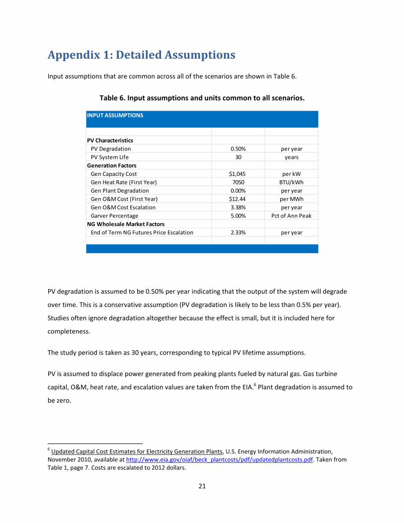
Input assumptions that are common across all of the scenarios are shown in Table 6.

Table 6. Input assumptions and units common to all scenarios.

PV degradation is assumed to be 0.50% per year indicating that the output of the system will degrade

over time. This is a conservative assumption (PV degradation is likely to be less than 0.5% per year).

Studies often ignore degradation altogether because the effect is small, but it is included here for

completeness.

The study period is taken as 30 years, corresponding to typical PV lifetime assumptions.

PV is assumed to displace power generated from peaking plants fueled by natural gas. Gas turbine

capital, O&M, heat rate, and escalation values are taken from the EIA.6 Plant degradation is assumed to

be zero.

6 Updated Capital Cost Estimates for Electricity Generation Plants, U.S. Energy Information Administration, November 2010, available at http://www.eia.gov/oiaf/beck_plantcosts/pdf/updatedplantcosts.pdf. Taken from Table 1, page 7. Costs are escalated to 2012 dollars.

INPUT ASSUMPTIONS

PV Characteristics

PV Degradation 0.50% per year

PV System Life 30 years

Generation Factors

Gen Capacity Cost $1,045 per kW

Gen Heat Rate (First Year) 7050 BTU/kWh

Gen Plant Degradation 0.00% per year

Gen O&M Cost (First Year) $12.44 per MWh

Gen O&M Cost Escalation 3.38% per year

Garver Percentage 5.00% Pct of Ann Peak

NG Wholesale Market Factors

End of Term NG Futures Price Escalation 2.33% per year

22

Costs for generation O&M are assumed to escalate at 3.38%, calculated from the change in Producer

Price Index (PPI) for the “Turbine and power transmission equipment manufacturing” industry7 over the

period 2004 to 2011.

Natural gas prices used in the fuel price savings value calculation are obtained from the NYMEX futures

prices. These prices, however, are only available for the first 12 years. Ideally, one would have 30 years

of futures prices. As a proxy for this value, it is assumed that escalation after year 12 is constant based

on historically long term prices to cover the entire 30 years of the PV service life (years 13 to 30). The

EIA published natural gas wellhead prices from 1922 to the present.8 It is assumed that the price of the

NG futures escalates at the same rate as the wellhead prices.9 A 30‐year time horizon is selected with

1981 gas prices at $1.98 per thousand cubic feet and 2011 prices at $3.95. This results in a natural gas

escalation rate of 2.33%.

7 PPI data is downloadable from the Bureau industry index selected was taken as the most representative of power generation O&M. BLS does publish an index for “Electric power generation” but this is assumed.

8 US Natural Gas Prices (Annual), EIA, release date 2/29/2012, available at http://www.eia.gov/dnav/ng/ng_pri_sum_dcu_nus_m.htm.

9 The exact number could be determined by obtaining over‐the‐counter NG forward prices.

23

Appendix2:Methodologies

Overview

The methodologies used in the present project drew upon studies performed by CPR for other states

and utilities. In these studies, the key value components provided by PV were determined by CPR, using

utility‐provided data and other economic data.

The ability to determine value on a site‐specific basis is essential to these studies. For example, the T&D

Capacity Value component depends upon the ability of PV to reduce peak loads on the circuits. An

analysis of this value, then, requires:

Hour by hour loads on distribution circuits of interest.

Hourly expected PV outputs corresponding to the location of these circuits and expected PV

system designs.

Local distribution expansion plan costs and load growth projections.

UnitsofResults

The discounting convention assumed throughout the report is that energy‐related values occur at the

end of each year and that capacity‐related values occur immediately (i.e., no discounting is required).10

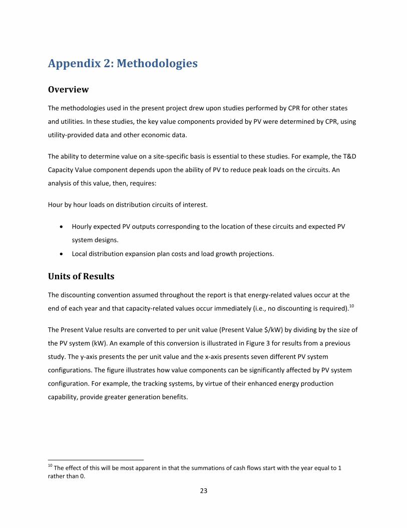
The Present Value results are converted to per unit value (Present Value $/kW) by dividing by the size of

the PV system (kW). An example of this conversion is illustrated in Figure 3 for results from a previous

study. The y‐axis presents the per unit value and the x‐axis presents seven different PV system

configurations. The figure illustrates how value components can be significantly affected by PV system

configuration. For example, the tracking systems, by virtue of their enhanced energy production

capability, provide greater generation benefits.

10 The effect of this will be most apparent in that the summations of cash flows start with the year equal to 1 rather than 0.

24

Figure 3. Sample results.

The present value results per unit of capacity ($/kW) are converted to levelized value results per unit of

energy ($/MWh) by dividing present value results by the total annual energy produced by the PV system

and then multiplying by an economic factor.

PVProductionandLossSavings

PVSystemOutput

An accurate PV value analysis begins with a detailed estimate of PV system output. Some of the energy‐

based value components may only require the total amount of energy produced per year. Other value

components, however, such as the energy loss savings and the capacity‐based value components,

require hourly PV system output in order to determine the technical match between PV system output

and the load. As a result, the PV value analysis requires time‐, location‐, and configuration‐specific PV

system output data.

For example, suppose that a utility wants to determine the value of a 1 MW fixed PV system oriented at

a 30° tilt facing in the southwest direction located at distribution feeder “A”. Detailed PV output data

that is time‐ and location‐specific is required over some historical period, such as from Jan. 1, 2001 to

Dec. 31, 2010.

25

Methodology

It would be tempting to use a representative year data source such as NREL’s Typical Meteorological

Year (TMY) data for purposes of performing a PV value analysis. While these data may be representative

of long‐term conditions, they are, by definition, not time‐correlated with actual distribution line loading

on an hourly basis and are therefore not usable in hourly side‐by‐side comparisons of PV and load. Peak

substation loads measured, say, during a mid‐August five‐day heat wave must be analyzed alongside PV

data that reflect the same five‐day conditions. Consequently, a technical analysis based on anything

other than time‐ and location‐correlated solar data may give incorrect results.

CPR’s SolarAnywhere® and PVSimulator™ software services will be employed under this project to

create time‐correlated PV output data. SolarAnywhere is a solar resource database containing almost 14

years of time‐ and location‐specific, hourly insolation data throughout the continental U.S. and Hawaii.

PVSimulator, available in the SolarAnywhere Toolkit, is a PV system modeling service that uses this

hourly resource data and user‐defined physical system attributes in order to simulate configuration‐

specific PV system output.

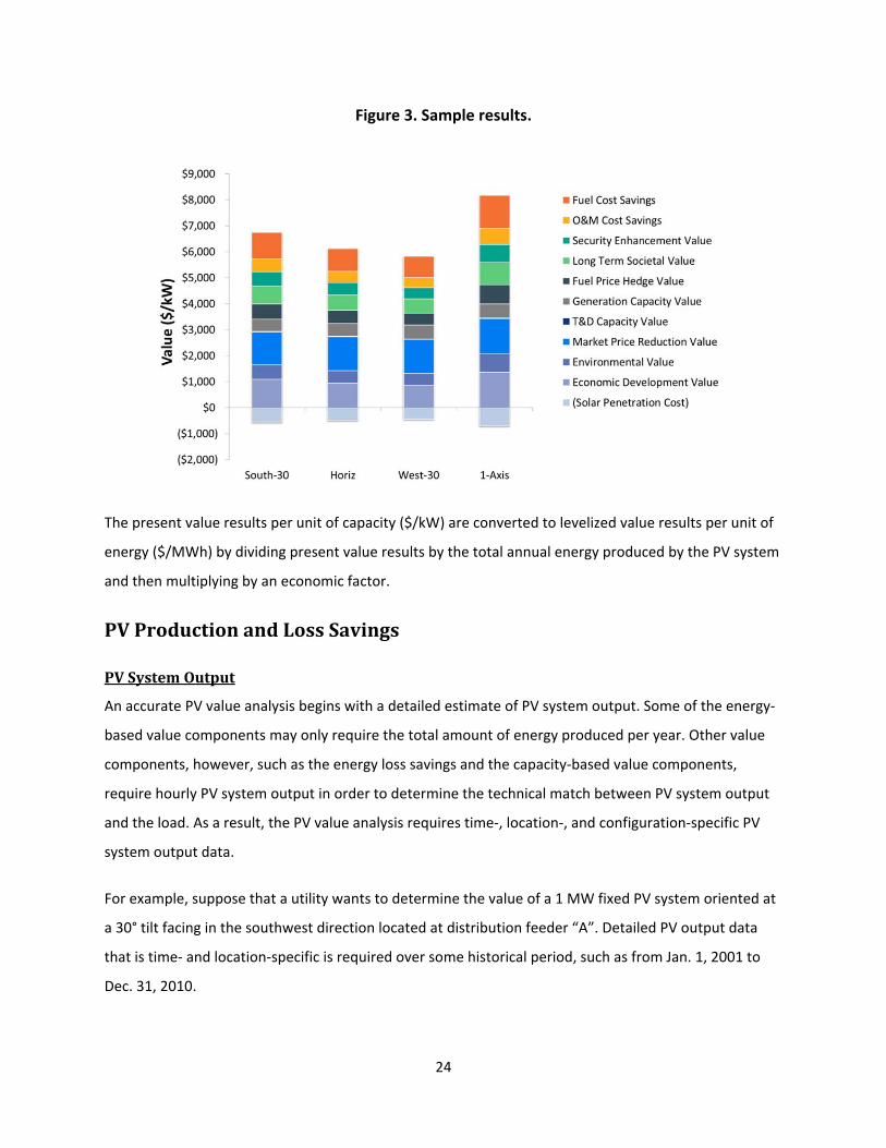
The SolarAnywhere data grid web interface is available at www.SolarAnywhere.com (Figure 4). The

structure of the data allows the user to perform a detailed technical assessment of the match between

PV system output and load data (even down to a specific feeder). Together, these two tools enable the

evaluation of the technical match between PV system output and loads for any PV system size and

orientation.

Previous PV value analyses were generally limited to a small number of possible PV system

configurations due to the difficulty in obtaining time‐ and location‐specific solar resource data. This new

value analysis software service, however, will integrate seamlessly with SolarAnywhere and

PVSimulator. This will allow users to readily select any PV system configuration. This will allow for the

evaluation of a comprehensive set of scenarios with essentially no additional study cost.

26

Figure 4. SolarAnywhere data selection map.

LossSavings

Introduction

Distributed resources reduce system losses because they produce power in the same location that the

power is consumed, bypassing the T&D system and avoiding the associated losses.

Loss savings are not treated as a stand‐alone benefit under the convention used in this methodology.

Rather, the effect of loss savings is included separately for each value component. For example, in the

section that covers the calculation of Energy Value, the quantity of energy saved by the utility includes

both the energy produced by PV and the amount that would have been lost due to heating in the wires

if the load were served from a remote source. The total energy that would have been procured by the

utility equals the PV energy plus avoided line losses. Loss savings can be considered a sort of “adder” for

each benefit component.

27

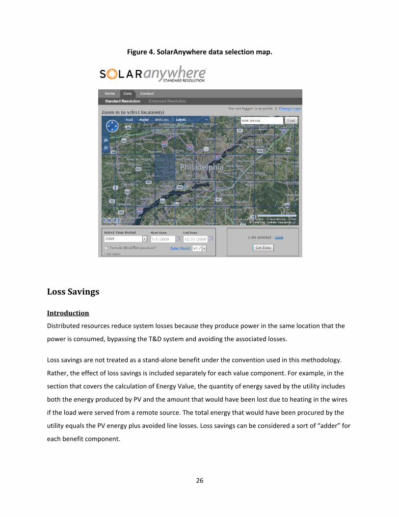
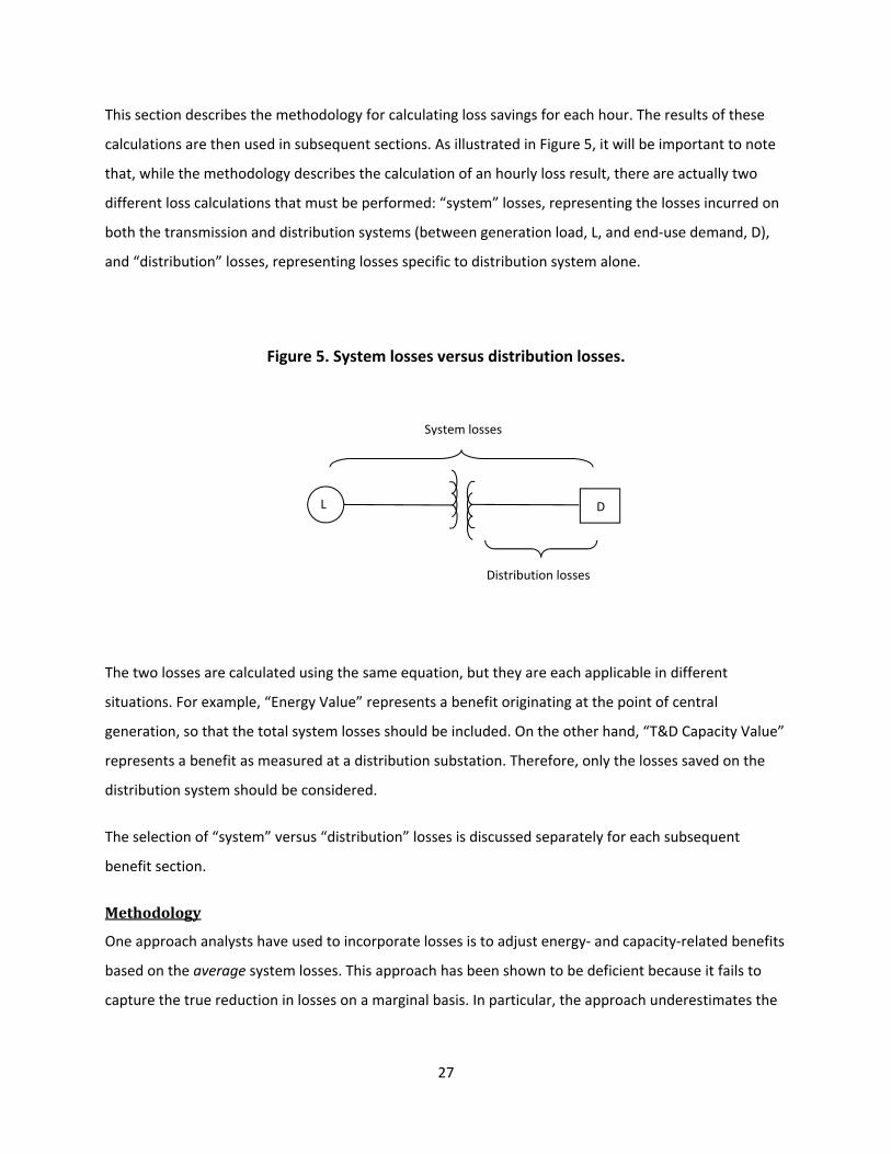
This section describes the methodology for calculating loss savings for each hour. The results of these

calculations are then used in subsequent sections. As illustrated in Figure 5, it will be important to note

that, while the methodology describes the calculation of an hourly loss result, there are actually two

different loss calculations that must be performed: “system” losses, representing the losses incurred on

both the transmission and distribution systems (between generation load, L, and end‐use demand, D),

and “distribution” losses, representing losses specific to distribution system alone.

Figure 5. System losses versus distribution losses.

The two losses are calculated using the same equation, but they are each applicable in different

situations. For example, “Energy Value” represents a benefit originating at the point of central

generation, so that the total system losses should be included. On the other hand, “T&D Capacity Value”

represents a benefit as measured at a distribution substation. Therefore, only the losses saved on the

distribution system should be considered.

The selection of “system” versus “distribution” losses is discussed separately for each subsequent

benefit section.

Methodology

One approach analysts have used to incorporate losses is to adjust energy‐ and capacity‐related benefits

based on the average system losses. This approach has been shown to be deficient because it fails to

capture the true reduction in losses on a marginal basis. In particular, the approach underestimates the

L D

Distribution losses

System losses

28

reduction in losses due to a peaking resource like PV. Results from earlier studies demonstrated that loss

savings calculations may be off by more than a factor of two if not performed correctly [6].

For this reason, the present methodology will incorporate a calculation of loss savings on a marginal

basis, taking into account the status of the utility grid when the losses occur. Clean Power Research has

previously developed methodologies based on the assumption that the distributed PV resource is small

relative to the load (e.g., [6], [9]). CPR has recently completed new research that expands this

methodology so that loss savings can now be determined for any level of PV penetration.

FuelCostSavingsandO&MCostSavings

Introduction

Fuel Cost Savings and O&M Cost Savings are the benefits that utility participants derive from using

distributed PV generation to offset wholesale energy purchases or reduce generation costs. Each kWh

generated by PV results in one less unit of energy that the utility needs to purchase or generate. In

addition, distributed PV reduces system losses so that the cost of the wholesale generation that would

have been lost must also be considered. The capacity value of generation is treated in a separate

section.

Methodology

These values can be calculated by multiplying PV system output times the cost of the generation on the

margin for each hour, summing for all hours over the year, and then discounting the results for each

year over the life of the PV system.

There are two approaches to obtaining the marginal cost data. One approach is to obtain the marginal

costs based on historical or projected market prices. The second approach is to obtain the marginal

costs based on the cost of operating a representative generator that is on the margin.

Initially, it may be appealing to take the approach of using market prices. There are, however, several

difficulties with this approach. One difficulty is that these tend to be hourly prices and thus require

hourly PV system output data in order to calculate the economic value. This difficulty can be addressed

by using historical prices and historical PV system output to evaluate what results would have been in

the past and then escalating the results for future projections. A more serious difficulty is that, while

hourly market prices could be projected for a few years into the future, the analysis needs to be

29

performed over a much longer time period (typically 30 years). It is difficult to accurately project hourly

market prices 30 years into the future.

A more robust approach is to explicitly specify the marginal generator and then to calculate the cost of

the generation from this unit. This is often a Combined Cycle Gas Turbine (CCGT) powered using natural

gas (e.g., [6]). This approach includes the assumption that PV output always displaces energy from the

same marginal unit. Given the uncertainties and complications in market price projections, the second

approach is taken.

Fuel Cost Savings and O&M Cost Savings equals the sum of the discounted fuel cost savings and the

discounted O&M cost savings.

SecurityEnhancementValue

Because solar generation is closely correlated with load in much of the US, including New Jersey and

Pennsylvania [26], the injection of solar energy near point of use can deliver effective capacity, and

therefore reduce the risk of the power outages and rolling blackouts that are caused by high demand

and resulting stresses on the transmission and distribution systems.

The effective capacity value of PV accrues to the ratepayer (see above) both at the transmission and

distribution levels. It is thus possible to argue that the reserve margins required by regulators would

account for this new capacity, hence that no increased outage risk reduction capability would occur

beyond the pre‐PV conditions. This is the reason this value item above is not included as one of the

directly quantifiable attributes of PV.

On the other hand there is ample evidence that during heat wave‐driven extreme conditions, the

availability of PV is higher than suggested by the effective capacity (reflecting of all conditions) ‐‐ e.g.,

see [27], [28], on the subject of major western and eastern outages, and [29] on the subject of localized

rolling blackouts. In addition, unlike conventional centralized generation injecting electricity (capacity) at

specific points on the grid, PV acts as a load modulator that provides immediate stress relief throughout

the grid where stress exists due to high‐demand conditions. It is therefore possible to argue that, all

conditions remaining the same in terms of reserve margins, a load‐side dispersed PV resource would

mitigate issues leading to high‐demand‐driven localized and regional outages.

30

Losses resulting from power outages are generally not a utility’s (ratepayers’) responsibility: society pays

the price, via losses of goods and business, compounded impacts on the economy and taxes, insurance

premiums, etc. The total cost of all power outages from all causes to the US economy has been

estimated at $100 billion per year (Gellings & Yeager, 2004). Making the conservative assumption that a

small fraction of these outages, 5%, are of the high‐demand stress type that can be effectively mitigated

by dispersed solar generation at a capacity penetration of 15%,11 it is straightforward to calculate, as

shown below, that, nationally, the value of each kWh generated by such a dispersed solar base would be

of the order of $20/MWh to the taxpayer.

The US generating capacity is roughly equal to 1000 GW. At 15% capacity penetration, taking a national

average of 1500 kWh (slightly higher nationwide than PA and NJ) generated per year per installed kW,

PV would generate 225,000 GWh/year. By reducing the risk of outage by 5%, the value of this energy

would thus be worth $5 billion, amounting to $20 per PV‐generated MWh.

This national value of $20 per MWh was taken for the present study because the underlying estimate of

cost was available on a national basis. In reality, there would be state‐level differences from this

estimate, but these are not available.

LongTermSocietalValue

This item is an attempt to place a present‐value $/MWh on the generally well accepted argument that

solar energy is a good investment for our children and grandchildren’s well‐being. Considering:

1. The rapid growth of large new world economies and the finite reserves of conventional fuels

now powering the world economies, it is likely that fuel prices will continue to rise

exponentially fast for the long term beyond the 30‐year business life cycle considered here.

2. The known very slow degradation of the leading (silicon) PV technology, many PV systems

installed today will continue to generate power at costs unaffected by the world fuel

markets after their guaranteed lifetimes of 25‐30 years

One approach to quantify this type of long‐view attribute has been to apply a very low societal discount

rate (e.g., 2% or less, see [25]) to mitigate the fact that the present‐day importance of long‐term

expenses/benefits is essentially ignored in business as usual practice. This is because discount rates are

11 Much less than that would have prevented the 2003 NE blackout. See [30].

31

used to quantify the present worth of future events and that, and therefore, long‐term risks and

attributes are largely irrelevant to current decision making.

Here a less controversial approach is proposed by arguing that, on average, PV installation will deliver,

on average, a minimum of 10 extra years of essentially free energy production beyond the life cycle

considered in this study.

The present value of these extra 10 years, all other assumptions on fuel cost escalation, inflation,

discount rate, PV output degradation, etc. remaining the same, amounts to ~ $25/MWh for all the

cities/PJM hubs considered in this study.

FuelPriceHedgeValue

Introduction

Solar‐based generation is insensitive to the volatility of fuel prices while fossil‐based generation is

directly tied to fuel prices. Solar generation, therefore, offers a “hedge” against fuel price volatility. One

way this has been accounted for is to quantify the value of PV’s hedge against fluctuating natural gas

prices [6].

Methodology

The key to calculating the Fuel Price Hedge Value is to effectively convert the fossil‐based generation

investment from one that has substantial fuel price uncertainty to one that has no fuel price

uncertainty. This can be accomplished by entering into a binding commitment to purchase a lifetime’s

worth of fuel to be delivered as needed. The utility could set aside the entire fuel cost obligation up

front, investing it in risk‐fee securities to be drawn from each year as required to meet the obligation.

The approach uses two financial instruments: risk‐free, zero‐coupon bonds12 and a set of natural gas

futures contracts.

Consider how this might work. Suppose that the CCGT operator wants to lock in a fixed price contract

for a sufficient quantity of natural gas to operate the plant for one month, one year in the future. First,

the operator would determine how much natural gas will be needed. If E units of electricity are to be

generated and the heat rate of the plant is H, E * H BTUs of natural gas will be needed. Second, if the

corresponding futures price of this natural gas is PNG Futures (in $ per BTU), then the operator will need E *

12 A zero coupon bond does not make any periodic interest payments.

32

H * PNG Futures dollars to purchase the natural gas one year from now. Third, the operator needs to set the

money aside in a risk‐free investment, typically a risk‐free bond (rate‐of‐return of rrisk‐free percent) to

guarantee that the money will be available when it is needed one year from now. Therefore, the

operator would immediately enter into a futures contract and purchase E * H * PNG Futures / (1+ rrisk‐free)

dollars worth of risk‐free, zero‐coupon bonds in order to guarantee with certainty that the financial

commitment (to purchase the fuel at the contract price at the specified time) will be satisfied.13

This calculation is repeated over the life of the plant to calculate the Fuel Price Hedge value.

GenerationCapacityValue

Introduction

Generation Capacity Value is the benefit from added capacity provided to the generation system by

distributed PV. Two different approaches can be taken to evaluating the Generation Capacity Value

component. One approach is to obtain the marginal costs based on market prices. The second approach

is to estimate the marginal costs based on the cost of operating a representative generator that is on

the margin, typically a Combined Cycle Gas Turbine (CCGT) powered by natural gas.

Methodology

The second approach is taken here for purposes of simplicity. Future version of the software service may

add a market price option.

Once the cost data for the fully‐dispatchable CCGT are obtained, the match between PV system output

and utility loads needs to be determined in order to determine the effective value of the non‐

dispatchable PV resource. CPR developed a methodology to calculate the effective capacity of a PV

system to the utility generation system (see [10] and [11]) and Perez advanced this method and called it

the Effective Load Carrying Capability (ELCC) [12]. The ELCC method has been identified by the utility

industry as one of the preferable methods to evaluate PV capacity [13] and has been applied to a variety

of places, including New York City [14].

The ELCC is a statistical measure of effective capacity. The ELCC of a generating unit in a utility grid is

defined as the load increase (MW) that the system can carry while maintaining the designated reliability

13 [E * H * PNG Futures / (1+ rrisk‐free)] * (1+ rrisk‐free) = E * H * PNG Futures

33

criteria (e.g., constant loss of load probability). The ELCC is obtained by analyzing a statistically

significant time series of the unit's output and of the utility's power requirements.

Generation Capacity Value equals the capital cost ($/MW) of the displaced generation unit times the

effective capacity provided by the PV.

T&DCapacityValue

Introduction

The benefit that can be most affected by the PV system’s location is the T&D Capacity Value. The T&D

Capacity Value depends on the existence of location‐specific projected expansion plan costs to ensure

reliability over the coming years as the loads grow. Capacity‐constrained areas where loads are expected

to reach critical limits present more favorable locations for PV to the extent that PV will relieve the

constraints, providing more value to the utility than those areas where capacity is not constrained.

Distributed PV generation reduces the burden on the distribution system. It appears as a “negative load”

during the daylight hours from the perspective of the distribution operator. Distributed PV may be

considered equivalent to distribution capacity from the perspective of the distribution planner, provided

that PV generation occurs at the time of the local distribution peak.

Distributed PV capacity located in an area of growing loads allows a utility planner to defer capital

investments in distribution equipment such as substations and lines. The value is determined by the

avoided cost of money due to the capital deferral.

Methodology

It has been demonstrated that the T&D Capacity Value can be quantified in a two‐step process. The first

step is to perform an economic screening of all areas to determine the expansion plan costs and load

growth rates for each planning area. The second step is to perform a technical load‐matching analysis

for the most promising locations [18].

MarketPriceReductionValue

Two cost savings occur when distributed PV generation is deployed in a market that is structured where

the last unit of generation sets the price for all generation and the price is an increasing function of load.

First, there is the direct savings that occur due to a reduction in load. This is the same as the value of

34

energy provided at the market price of power. Second, there is the indirect value of market price

reduction. Distributed generation reduces market demand and this results in lower prices to all those

purchasing power from the market. This section outlines how to calculate the market savings value.

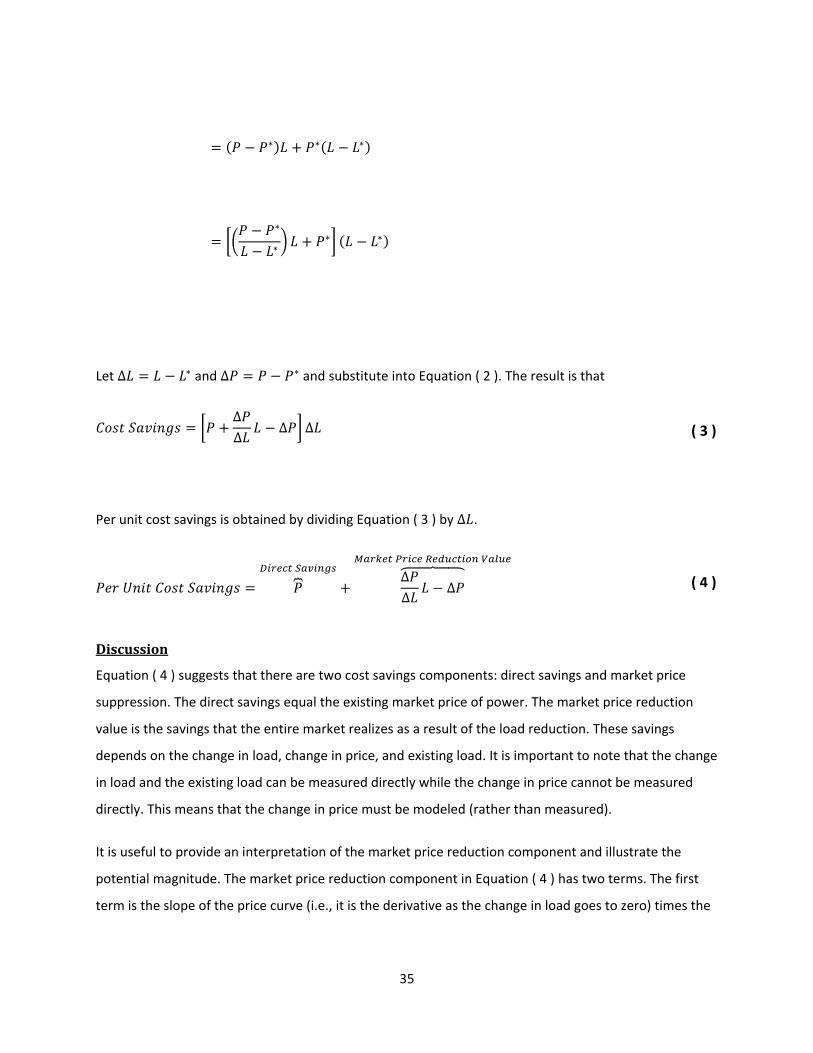
CostSavings

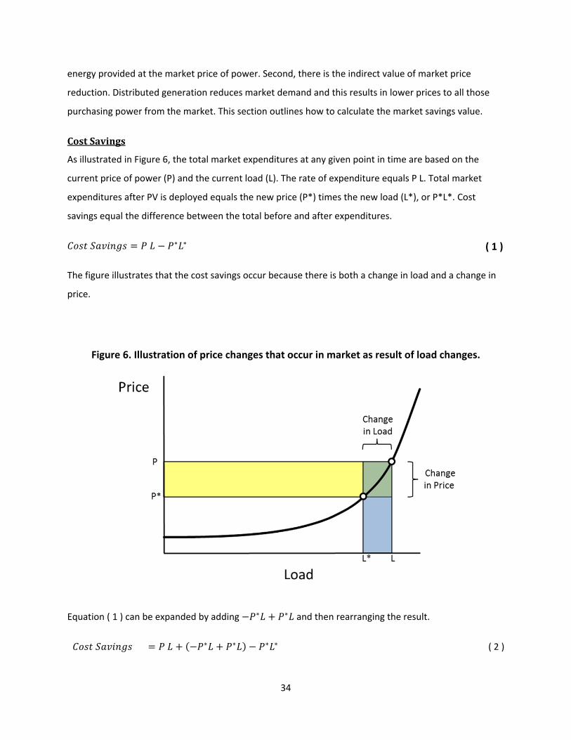
As illustrated in Figure 6, the total market expenditures at any given point in time are based on the

current price of power (P) and the current load (L). The rate of expenditure equals P L. Total market

expenditures after PV is deployed equals the new price (P*) times the new load (L*), or P*L*. Cost

savings equal the difference between the total before and after expenditures.

∗ ∗ ( 1 )

The figure illustrates that the cost savings occur because there is both a change in load and a change in

price.

Figure 6. Illustration of price changes that occur in market as result of load changes.

Equation ( 1 ) can be expanded by adding ∗ ∗ and then rearranging the result.

∗ ∗ ∗ ∗ ( 2 )

35

∗ ∗ ∗

∗

∗∗ ∗

Let ∆ ∗ and ∆ ∗ and substitute into Equation ( 2 ). The result is that

∆∆

∆ ∆ ( 3 )

Per unit cost savings is obtained by dividing Equation ( 3 ) by ∆ .

∆∆

∆ ( 4 )

Discussion

Equation ( 4 ) suggests that there are two cost savings components: direct savings and market price

suppression. The direct savings equal the existing market price of power. The market price reduction

value is the savings that the entire market realizes as a result of the load reduction. These savings

depends on the change in load, change in price, and existing load. It is important to note that the change

in load and the existing load can be measured directly while the change in price cannot be measured

directly. This means that the change in price must be modeled (rather than measured).

It is useful to provide an interpretation of the market price reduction component and illustrate the

potential magnitude. The market price reduction component in Equation ( 4 ) has two terms. The first

term is the slope of the price curve (i.e., it is the derivative as the change in load goes to zero) times the

36

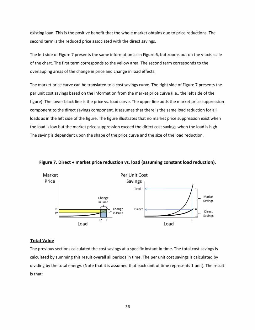
existing load. This is the positive benefit that the whole market obtains due to price reductions. The

second term is the reduced price associated with the direct savings.

The left side of Figure 7 presents the same information as in Figure 6, but zooms out on the y‐axis scale

of the chart. The first term corresponds to the yellow area. The second term corresponds to the

overlapping areas of the change in price and change in load effects.

The market price curve can be translated to a cost savings curve. The right side of Figure 7 presents the

per unit cost savings based on the information from the market price curve (i.e., the left side of the

figure). The lower black line is the price vs. load curve. The upper line adds the market price suppression

component to the direct savings component. It assumes that there is the same load reduction for all

loads as in the left side of the figure. The figure illustrates that no market price suppression exist when

the load is low but the market price suppression exceed the direct cost savings when the load is high.

The saving is dependent upon the shape of the price curve and the size of the load reduction.

Figure 7. Direct + market price reduction vs. load (assuming constant load reduction).

TotalValue

The previous sections calculated the cost savings at a specific instant in time. The total cost savings is

calculated by summing this result overall all periods in time. The per unit cost savings is calculated by

dividing by the total energy. (Note that it is assumed that each unit of time represents 1 unit). The result

is that:

37

∑ ∆∆ ∆ ∆

∑ ∆ ( 5 )

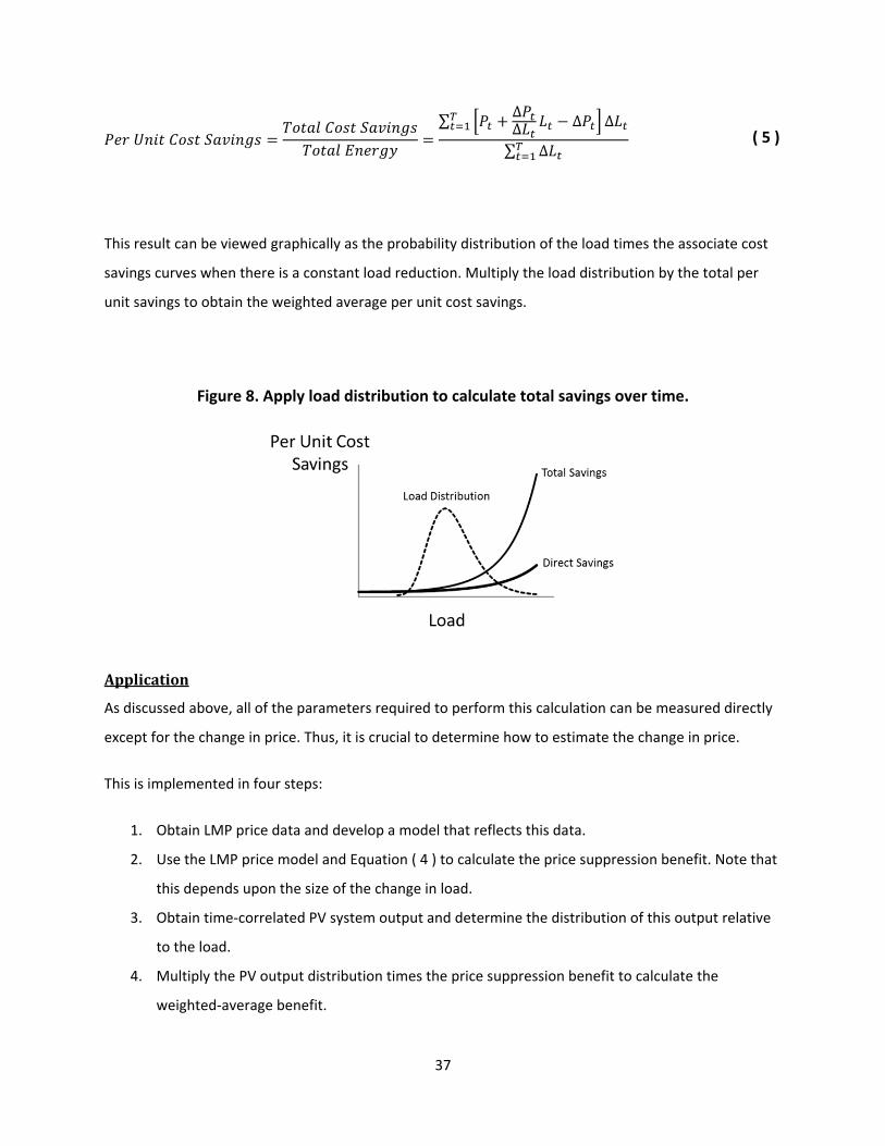
This result can be viewed graphically as the probability distribution of the load times the associate cost

savings curves when there is a constant load reduction. Multiply the load distribution by the total per

unit savings to obtain the weighted average per unit cost savings.

Figure 8. Apply load distribution to calculate total savings over time.

Application

As discussed above, all of the parameters required to perform this calculation can be measured directly

except for the change in price. Thus, it is crucial to determine how to estimate the change in price.

This is implemented in four steps:

1. Obtain LMP price data and develop a model that reflects this data.

2. Use the LMP price model and Equation ( 4 ) to calculate the price suppression benefit. Note that

this depends upon the size of the change in load.

3. Obtain time‐correlated PV system output and determine the distribution of this output relative

to the load.

4. Multiply the PV output distribution times the price suppression benefit to calculate the

weighted‐average benefit.

38

Historical LMP and time‐ and location‐correlated PV output data are required to perform the analysis.

LMPs are obtained from the market and the PV output data are obtained by simulating time‐ and

location‐specific PV output using SolarAnywhere.

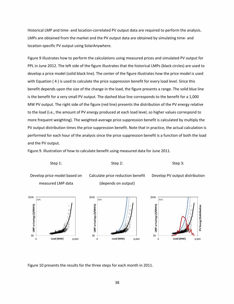
Figure 9 illustrates how to perform the calculations using measured prices and simulated PV output for

PPL in June 2012. The left side of the figure illustrates that the historical LMPs (black circles) are used to

develop a price model (solid black line). The center of the figure illustrates how the price model is used

with Equation ( 4 ) is used to calculate the price suppression benefit for every load level. Since this

benefit depends upon the size of the change in the load, the figure presents a range. The solid blue line

is the benefit for a very small PV output. The dashed blue line corresponds to the benefit for a 1,000

MW PV output. The right side of the figure (red line) presents the distribution of the PV energy relative

to the load (i.e., the amount of PV energy produced at each load level, so higher values correspond to

more frequent weighting). The weighted‐average price suppression benefit is calculated by multiply the

PV output distribution times the price suppression benefit. Note that in practice, the actual calculation is

performed for each hour of the analysis since the price suppression benefit is a function of both the load

and the PV output.

Figure 9. Illustration of how to calculate benefit using measured data for June 2011.

Step 1: Step 2: Step 3:

Develop price model based on

measured LMP data

Calculate price reduction benefit

(depends on output)

Develop PV output distribution

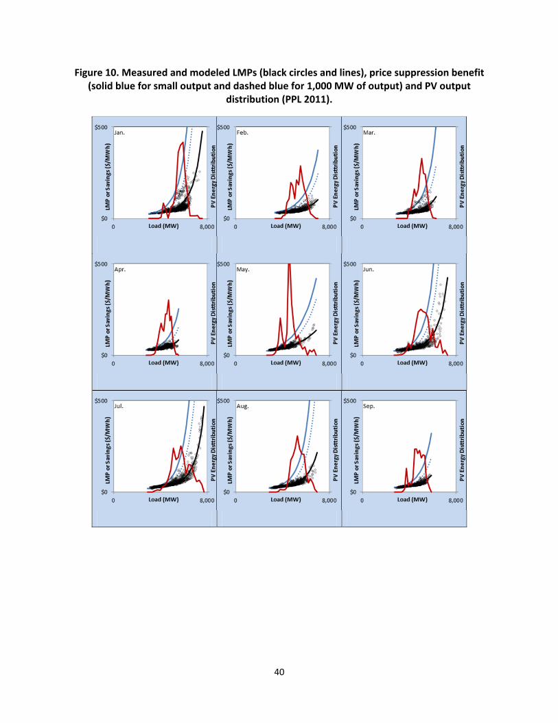
Figure 10 presents the results for the three steps for each month in 2011.

39

40

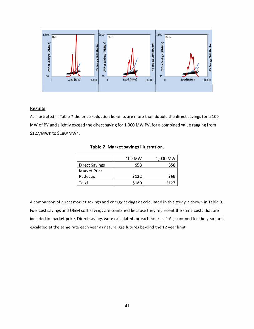
Figure 10. Measured and modeled LMPs (black circles and lines), price suppression benefit (solid blue for small output and dashed blue for 1,000 MW of output) and PV output

distribution (PPL 2011).

41

Results

As illustrated in Table 7 the price reduction benefits are more than double the direct savings for a 100

MW of PV and slightly exceed the direct saving for 1,000 MW PV, for a combined value ranging from

$127/MWh to $180/MWh.

Table 7. Market savings illustration.

100 MW 1,000 MW

Direct Savings $58 $58

Market Price Reduction $122 $69

Total $180 $127

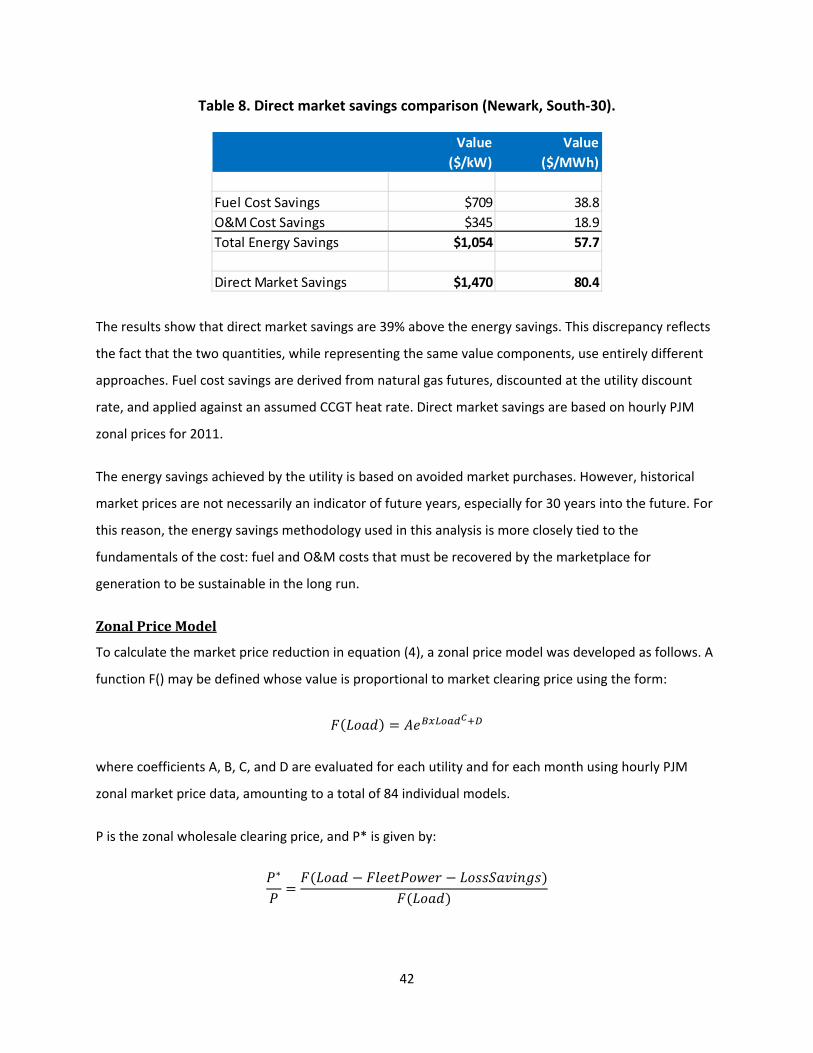
A comparison of direct market savings and energy savings as calculated in this study is shown in Table 8.

Fuel cost savings and O&M cost savings are combined because they represent the same costs that are

included in market price. Direct savings were calculated for each hour as P∙∆L, summed for the year, and

escalated at the same rate each year as natural gas futures beyond the 12 year limit.

42

Table 8. Direct market savings comparison (Newark, South‐30).

The results show that direct market savings are 39% above the energy savings. This discrepancy reflects

the fact that the two quantities, while representing the same value components, use entirely different

approaches. Fuel cost savings are derived from natural gas futures, discounted at the utility discount

rate, and applied against an assumed CCGT heat rate. Direct market savings are based on hourly PJM

zonal prices for 2011.

The energy savings achieved by the utility is based on avoided market purchases. However, historical

market prices are not necessarily an indicator of future years, especially for 30 years into the future. For

this reason, the energy savings methodology used in this analysis is more closely tied to the

fundamentals of the cost: fuel and O&M costs that must be recovered by the marketplace for

generation to be sustainable in the long run.

ZonalPriceModel

To calculate the market price reduction in equation (4), a zonal price model was developed as follows. A

function F() may be defined whose value is proportional to market clearing price using the form:

where coefficients A, B, C, and D are evaluated for each utility and for each month using hourly PJM

zonal market price data, amounting to a total of 84 individual models.

P is the zonal wholesale clearing price, and P* is given by:

∗

Value Value

($/kW) ($/MWh)

Fuel Cost Savings $709 38.8

O&M Cost Savings $345 18.9

Total Energy Savings $1,054 57.7

Direct Market Savings $1,470 80.4

43

The market price reduction (in $/MWh) is calculated using the relevant term in Equation (4) and

multiplying by the change in load, including loss savings.

EnvironmentalValue

Introduction

It is well established that the environmental impact of PV is considerably smaller than that of fossil‐

based generation since PV is able to displace pollution associated with drilling/mining, and power plant

emissions [15].

Methodology

There are two general approaches to quantifying the Environmental Value of PV: a regulatory cost‐

based approach and an environmental/health cost‐based approach.

The regulatory cost‐based approach values the Environmental Value of PV based on the price of

Renewable Energy Credits (RECs) or Solar Renewable Energy Credits (SRECs) that would otherwise have

to be purchased to satisfy state Renewable Portfolio Standards (RPS). These costs are a preliminary

legislative attempt to quantify external costs. They represent actual business costs faced by utilities in

certain states.

An environmental/health cost‐based approach quantifies the societal costs resulting from fossil

generation. Each solar kWh displaces an otherwise dirty kWh and commensurately mitigates several of

the following factors: greenhouse gases, SOx/NOx emissions, mining degradations, ground water

contamination, toxic releases and wastes, etc., that are all present or postponed costs to society. Several

exhaustive studies have estimated the environmental/health cost of energy generated by fossil‐based

generation [16], [17]. The results from environmental/health cost‐based approach often vary widely and

can be controversial.

The environmental/health cost‐based approach was used for this study.

The environmental footprint of solar generation is considerably smaller than that of the fossil fuel

technologies generating most of our electricity (e.g., [19]). Utilities have to account for this

environmental impact to some degree today, but this is still only largely a potential cost to them. Rate‐

based Solar Renewable Energy Credits (SRECs) markets in New Jersey and Pennsylvania as a means to

meet Renewable Portfolio Standards (RPS) are a preliminary embodiment of including external costs,

44

but they are largely driven more by politically‐negotiated processes than by a reflection of inherent

physical realities. The intrinsic physical value of displacing pollution is real and quantifiable however:

depending on the current generation mix, each solar kWh displaces an otherwise dirty kWh and

commensurately mitigates several of the following factors: greenhouse gases, SOx/NOx emissions,

mining degradations, ground water contamination, toxic releases and wastes, etc., which are all present

or postponed costs to society (i.e., the taxpayers).

The environmental value, EV, of each kWh produced by PV (i.e., not produced by another conventional

source) is given by:

Where ECi is the environmental cost of the displaced conventional generation technology and xi is the

proportion of this technology in the current energy mix.

Several exhaustive studies emanating from such diverse sources as the nuclear industry or the medical

community ([20], [21]) estimate the environmental/health cost of 1 MWh generated by coal at $90‐250,

while a [non‐shale14] natural gas MWh has an environmental cost of $30‐60.

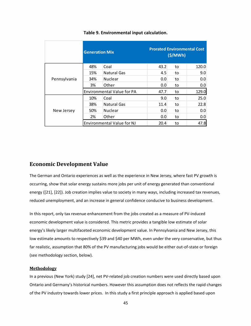
Considering New Jersey and Pennsylvania’s electrical generation mixes (Table 9) and assuming that (1)

nuclear energy is not displaced by PV at the assumed penetration level15 and (2) that all natural gas is

conventional, the environmental value of each MWh displaced by PV, hence the taxpayer benefit, is

estimated at $48 to $129 in Pennsylvania and $20 to $48 in New Jersey.

We retained a value near the lower range of these estimates for the present analysis.

14 Shale gas environmental footprint is likely higher both in terms of environment degradation and GHG emissions.

15 The study therefore ascribes no environmental value related to nuclear generation. Scenarios can certainly be designed in which nuclear generation would be displaced, in which case the environmental cost of nuclear generation would have to be considered. This is a complex and controversial subject that reflects the probability of catastrophic accidents and the environmental footprint of the existing uranium cycle. The fact that the environmental liability is assumed to be zero under the present study may therefore be considered a conservative case.

45

Table 9. Environmental input calculation.

EconomicDevelopmentValue

The German and Ontario experiences as well as the experience in New Jersey, where fast PV growth is

occurring, show that solar energy sustains more jobs per unit of energy generated than conventional

energy ([21], [22]). Job creation implies value to society in many ways, including increased tax revenues,

reduced unemployment, and an increase in general confidence conducive to business development.

In this report, only tax revenue enhancement from the jobs created as a measure of PV‐induced

economic development value is considered. This metric provides a tangible low estimate of solar

energy’s likely larger multifaceted economic development value. In Pennsylvania and New Jersey, this

low estimate amounts to respectively $39 and $40 per MWh, even under the very conservative, but thus

far realistic, assumption that 80% of the PV manufacturing jobs would be either out‐of‐state or foreign

(see methodology section, below).

Methodology

In a previous (New York) study [24], net PV‐related job creation numbers were used directly based upon

Ontario and Germany’s historical numbers. However this assumption does not reflects the rapid changes

of the PV industry towards lower prices. In this study a first principle approach is applied based upon

Generation Mix

48% Coal 43.2 to 120.0

15% Natural Gas 4.5 to 9.0

34% Nuclear 0.0 to 0.0

3% Other 0.0 to 0.0

Environmental Value for PA 47.7 to 129.0

10% Coal 9.0 to 25.0

38% Natural Gas 11.4 to 22.8

50% Nuclear 0.0 to 0.0

2% Other 0.0 to 0.0

Environmental Value for NJ 20.4 to 47.8

Pennsylvania

New Jersey

Prorated Environmental Cost

($/MWh)

46

the difference between the installed cost of PV and conventional generation: in essence this approach

quantifies the fact that part of the price premium paid for PV vs. conventional generation returns to the

local economy in the form of jobs hence tax.

Therefore, assuming that:

Turnkey PV costs $3,000 per kW vs. $1,000 per kW for combine cycle gas turbines (CCGT)

Turnkey PV cost is composed of 1/3 technology (modules & inverter/controls) and 2/3 structure

and installation and soft costs.

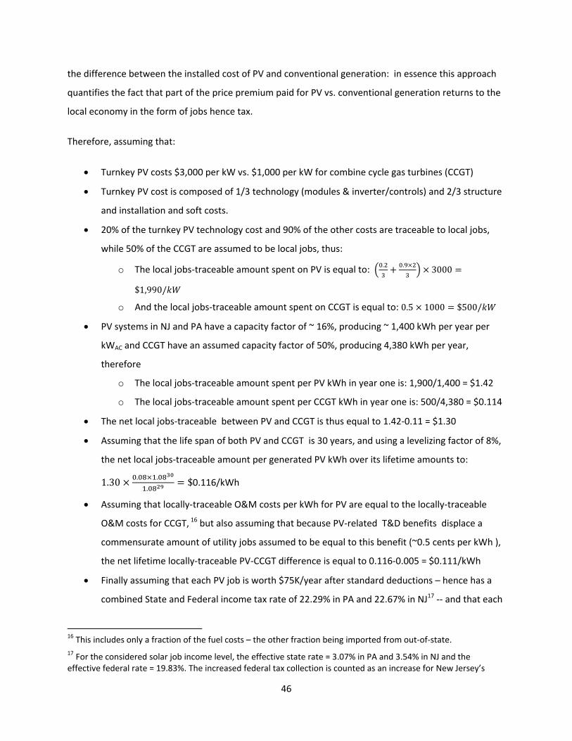
20% of the turnkey PV technology cost and 90% of the other costs are traceable to local jobs,

while 50% of the CCGT are assumed to be local jobs, thus:

o The local jobs‐traceable amount spent on PV is equal to: . .

3000

$1,990/

o And the local jobs‐traceable amount spent on CCGT is equal to: 0.5 1000 $500/

PV systems in NJ and PA have a capacity factor of ~ 16%, producing ~ 1,400 kWh per year per

kWAC and CCGT have an assumed capacity factor of 50%, producing 4,380 kWh per year,

therefore

o The local jobs‐traceable amount spent per PV kWh in year one is: 1,900/1,400 = $1.42

o The local jobs‐traceable amount spent per CCGT kWh in year one is: 500/4,380 = $0.114

The net local jobs‐traceable between PV and CCGT is thus equal to 1.42‐0.11 = $1.30

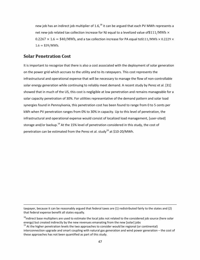
Assuming that the life span of both PV and CCGT is 30 years, and using a levelizing factor of 8%,

the net local jobs‐traceable amount per generated PV kWh over its lifetime amounts to:

1.30. .

.$0.116/kWh

Assuming that locally‐traceable O&M costs per kWh for PV are equal to the locally‐traceable

O&M costs for CCGT, 16 but also assuming that because PV‐related T&D benefits displace a

commensurate amount of utility jobs assumed to be equal to this benefit (~0.5 cents per kWh ),

the net lifetime locally‐traceable PV‐CCGT difference is equal to 0.116‐0.005 = $0.111/kWh

Finally assuming that each PV job is worth $75K/year after standard deductions – hence has a

combined State and Federal income tax rate of 22.29% in PA and 22.67% in NJ17 ‐‐ and that each

16 This includes only a fraction of the fuel costs – the other fraction being imported from out‐of‐state.

17 For the considered solar job income level, the effective state rate = 3.07% in PA and 3.54% in NJ and the effective federal rate = 19.83%. The increased federal tax collection is counted as an increase for New Jersey’s

47

new job has an indirect job multiplier of 1.6,18 it can be argued that each PV MWh represents a

net new‐job related tax collection increase for NJ equal to a levelized value of$111/MWh

0.2267 1.6 $40/MWh, and a tax collection increase for PA equal to$111/MWh 0.2229

1.6 $39/MWh.

SolarPenetrationCost

It is important to recognize that there is also a cost associated with the deployment of solar generation

on the power grid which accrues to the utility and to its ratepayers. This cost represents the

infrastructural and operational expense that will be necessary to manage the flow of non‐controllable

solar energy generation while continuing to reliably meet demand. A recent study by Perez et al. [31]

showed that in much of the US, this cost is negligible at low penetration and remains manageable for a

solar capacity penetration of 30%. For utilities representative of the demand pattern and solar load

synergies found in Pennsylvania, this penetration cost has been found to range from 0 to 5 cents per

kWh when PV penetration ranges from 0% to 30% in capacity. Up to this level of penetration, the

infrastructural and operational expense would consist of localized load management, [user‐sited]

storage and/or backup.19 At the 15% level of penetration considered in this study, the cost of

penetration can be estimated from the Perez et al. study18 at $10‐20/MWh.

taxpayer, because it can be reasonably argued that federal taxes are (1) redistributed fairly to the states and (2) that federal expense benefit all states equally.

18indirect base multipliers are used to estimate the local jobs not related to the considered job source (here solar energy) but created indirectly by the new revenues emanating from the new [solar] jobs 19 At the higher penetration levels the two approaches to consider would be regional (or continental) interconnection upgrade and smart coupling with natural gas generation and wind power generation – the cost of these approaches has not been quantified as part of this study.

48

MethodologyReferences

[1]. Hoff, T. E., Wenger, H. J., and Farmer, B. K. “Distributed Generation: An Alternative to Electric Utility

Investments in System Capacity”, Energy Policy 24(2):137‐147, 1996.

[2]. Hoff, T. E. Final Results Report with a Determination of Stacked Benefits of Both Utility‐Owned and

Customer‐Owned PV Systems: Deliverable 1.3.5.2, SMUD Report, 2002.

[3]. Hoff, T. E., and Margolis, R. Distributed Photovoltaics in New Jersey, NREL Report, 2003.

www.cleanpower.com/research/distributedgeneration/DistributedPVInNewJersey.pdf.

[4]. Hoff, T. E., Norris, B. L., and Wayne, G. Potential Economic Benefits of Distributed Photovoltaics to

the Nevada Power Company. Report, 2003.

www.cleanpower.com/Content/Documents/research/distributedgeneration/NevadaPower2003.pdf

[5]. Hoff, T. E. and Margolis, R. M. Moving Towards a More Comprehensive Framework to Evaluate

Distributed Photovoltaics. Report, 2005.

www.cleanpower.com/Content/Documents/research/customerPV/EvaluationFramework.pdf

[6]. Hoff, T.E., Perez, R., Braun, G., Kuhn, M., and Norris, B. The Value of Distributed Photovoltaics to

Austin Energy and the City of Austin, 2006.

www.cleanpower.com/Content/Documents/research/distributedgeneration/AE_PV_ValueReport.pdf.

[7]. Norris, B. L., Hoff, T. E., Perez, R. PV Value Analysis for We Energies, 2009.

[8]. Perez, R. Zweibel, K., and Hoff, T. E. “Solar Power Generation in the US: Too expensive, or a

bargain?” Submitted to Energy Policy. 2011.

[9]. Hoff, T. and Shugar, D. S., “The Value of Grid‐Support Photovoltaics In Reducing Distribution System

Losses”, IEEE Transactions on Energy Conversion, 10(9): 569‐576.,1995.

[10]. Garver, L. L. “Effective Load Carrying Capability of Generating Units. IEEE Transactions, Power

Apparatus and Systems.” Vol. Pas‐85, no. 8, 1966.

[11]. Hoff, T. “Calculating Photovoltaics' Value: A Utility Perspective,” IEEE Transactions on Energy

Conversion 3: 491‐495, 1988.

49

[12]. Perez, R., Seals, R., and Stewart, R. “Assessing the Load Matching Capability of Photovoltaics for US

Utilities Based Upon Satellite‐Derived Insolation Data”, IEEE Transactions, pp. 1146‐1149 (23d. PV

Specialists, Louisville, KY), 1993.

[13]. Hoff, T., Perez, R. Ross, JP, and Taylor, M. Photovoltaic Capacity Valuation Methods, Solar Electric

Power Association Report #02‐08, 2008.

[14]. Hoff, T. E. and Perez, R. Shining on the Big Apple: Satisfying New York City’s Peak Electrical Needs

with PV. Report, 2008.

www.cleanpower.com/Content/Documents/research/distributedgeneration/PVForNewYorkCity.pdf.

[15]. Fthenakis, V., Kim, H.C., Alsema, E., “Emissions from Photovoltaic Life Cycles”. Environmental

Science and Technology, 42(6): p. 2168‐2174, 2008.

[16]. Devezeaux J. G. “Environmental Impacts of Electricity Generation”. 25th Uranium Institute Annual

Symposium. London, UK, 2000.

[17]. Epstein, P. “Full cost accounting for the life cycle of coal”. Annals of the New York Academy of

Sciences, 2011.

[18]. Hoff, T. E. “Identifying Distributed Generation and Demand Side Management Investment

Opportunities”, The Energy Journal: 17(4), 1996.

[19]. Fthenakis, V., Kim, H.C., Alsema, E., 2008. Emissions from Photovoltaic Life Cycles. Environmental

Science and Technology, 42(6): p. 2168‐2174

[20]. Devezeaux J. G., 2000. Environmental Impacts of Electricity Generation. 25th Uranium Institute

Annual Symposium. London, UK (September, 2000).

[21]. Epstein, P. 2011. Full cost accounting for the life cycle of coal. Annals of the New York Academy of

Sciences. February, 2011.

[22]. Louw, B., J.E. Worren and T. Wohlgemut, 2010. Economic Impacts of Solar Energy in Ontario.

CLearSky Advisors Report (www.clearskyadvisors.com).

[23]. Ban‐Weiss G. et al., 2010 “Solar Energy Job Creation in California”, University of California at

Berkeley.

50

[24]. Perez, R., K. Zweibel and T.E. Hoff, (2011): Solar Power Generation in the US: Too Expensive, or a

Bargain? Journal of Energy Policy, 39 (2011), 7290‐7297.

[25]. Tol R.S.J., J. Guo, C.J. Hepburn, and D. Anthoff 2006. Discounting and the Social Cost of Carbon: a

Closer Look at Uncertainty, Environmental Science & Policy, 9, 205‐216, 207.

[26]. Perez, R., R. Margolis, M. Kmiecik, M. Schwab and M. Perez, (2006): Update: Effective Load

Carrying Capability of Photovoltaics in the United States. Proc. ASES Annual Conference, Denver, CO

[27]. Perez, R., R. Seals, H. Wenger, T. Hoff and C. Herig, 1997. PV as a Long‐Term Solution to Power

Outages. Case Study: The Great 1996 WSCC Power Outage. Proc. ASES Annual Conference, Washington,

DC.

[28]. Perez R., B. Collins, R. Margolis, T. Hoff, C. Herig J. Williams and S. Letendre, 2005. Solution to the

Summer Blackouts – How dispersed solar power generating systems can help prevent the next major

outage. Solar Today 19,4, July/August 2005 Issue, pp. 32‐35.

[29]. Letendre S. and R. Perez, 2006. Understanding the Benefits of Dispersed Grid‐Connected

Photovoltaics: From Avoiding the Next Major Outage to Taming Wholesale Power Markets. The

Electricity Journal, 19, 6, 64‐72.

[30]. Perez R., B. Collins, R. Margolis, T. Hoff, C. Herig J. Williams and S. Letendre, (2005) Solution to the

Summer Blackouts – How dispersed solar power generating systems can help prevent the next major

outage. Solar Today 19,4, July/August 2005 Issue, pp. 32‐35.

[31]. Perez, R., T. Hoff and M. Perez, (2010): Quantifying the Cost of High PV Penetration. Proc. of ASES National

Conference, Phoenix, AZ.

[32]. Felder, F. A., “Examining Electricity Price Suppression Due to Renewable Resources and Other Grid

Investments,” The Electricity Journal, Vol. 24, Issue 4, May 2011.

51

Appendix3:DetailedResults

52

Pittsburgh

Table A4‐ 1. Technical results, Pittsburgh.

Table A4‐ 2. Value ($/kW), Pittsburgh.

Table A4‐ 3. Levelized Value ($/MWh), Pittsburgh.

South‐30 Horiz West‐30 1‐AxisFleet Capacity (MWac) 475 475 475 475

Annual Energy Production (MWh) 716,621 631,434 595,373 892,905

Capacity Factor (%) 17% 15% 14% 21%

Generation Capacity (% of Fleet Capacity) 41% 43% 45% 48%

T&D Capacity (% of Fleet Capaccity) 31% 32% 32% 32%

South‐30 Horiz West‐30 1‐Axis

EnergyFuel Cost Savings $813 $719 $678 $1,011

O&M Cost Savings $396 $350 $331 $493

Total Energy Value $1,209 $1,069 $1,009 $1,503

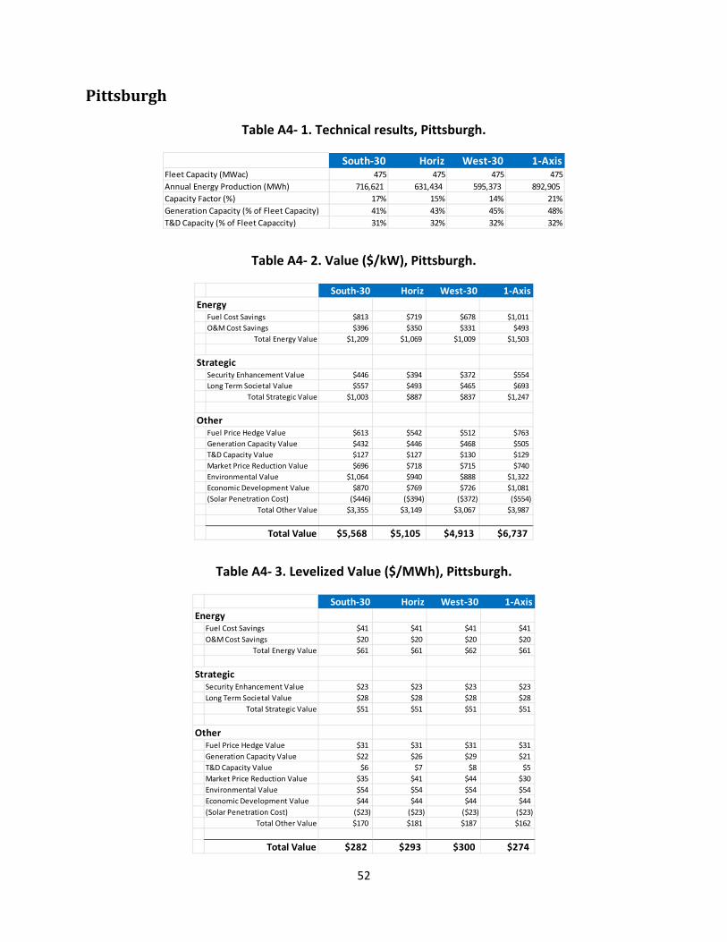
StrategicSecurity Enhancement Value $446 $394 $372 $554

Long Term Societal Value $557 $493 $465 $693

Total Strategic Value $1,003 $887 $837 $1,247

OtherFuel Price Hedge Value $613 $542 $512 $763

Generation Capacity Value $432 $446 $468 $505

T&D Capacity Value $127 $127 $130 $129

Market Price Reduction Value $696 $718 $715 $740

Environmental Value $1,064 $940 $888 $1,322

Economic Development Value $870 $769 $726 $1,081

(Solar Penetration Cost) ($446) ($394) ($372) ($554)

Total Other Value $3,355 $3,149 $3,067 $3,987

Total Value $5,568 $5,105 $4,913 $6,737


EnergyFuel Cost Savings $41 $41 $41 $41

O&M Cost Savings $20 $20 $20 $20

Total Energy Value $61 $61 $62 $61



Total Strategic Value $51 $51 $51 $51





Environmental Value $54 $54 $54 $54

Economic Development Value $44 $44 $44 $44


Total Other Value $170 $181 $187 $162

Total Value $282 $293 $300 $274

53

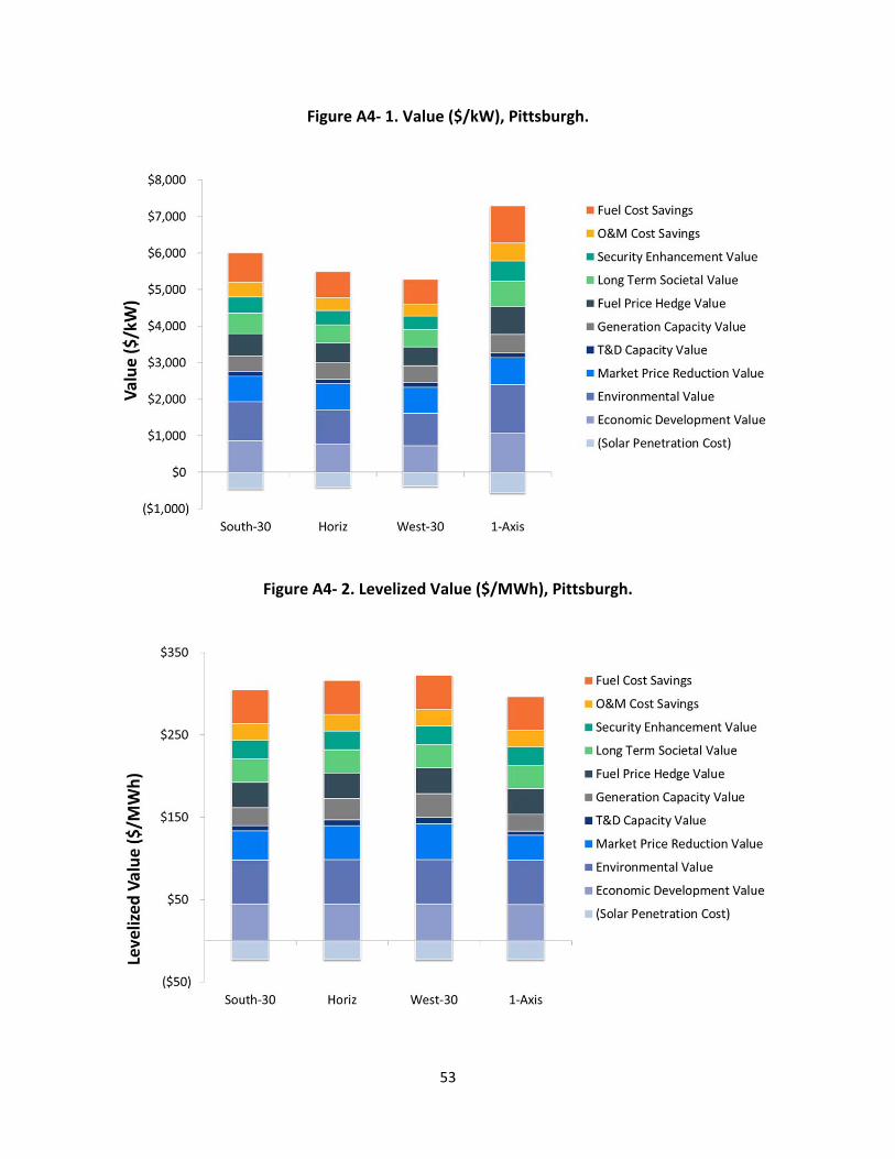
Figure A4‐ 1. Value ($/kW), Pittsburgh.

Figure A4‐ 2. Levelized Value ($/MWh), Pittsburgh.

54

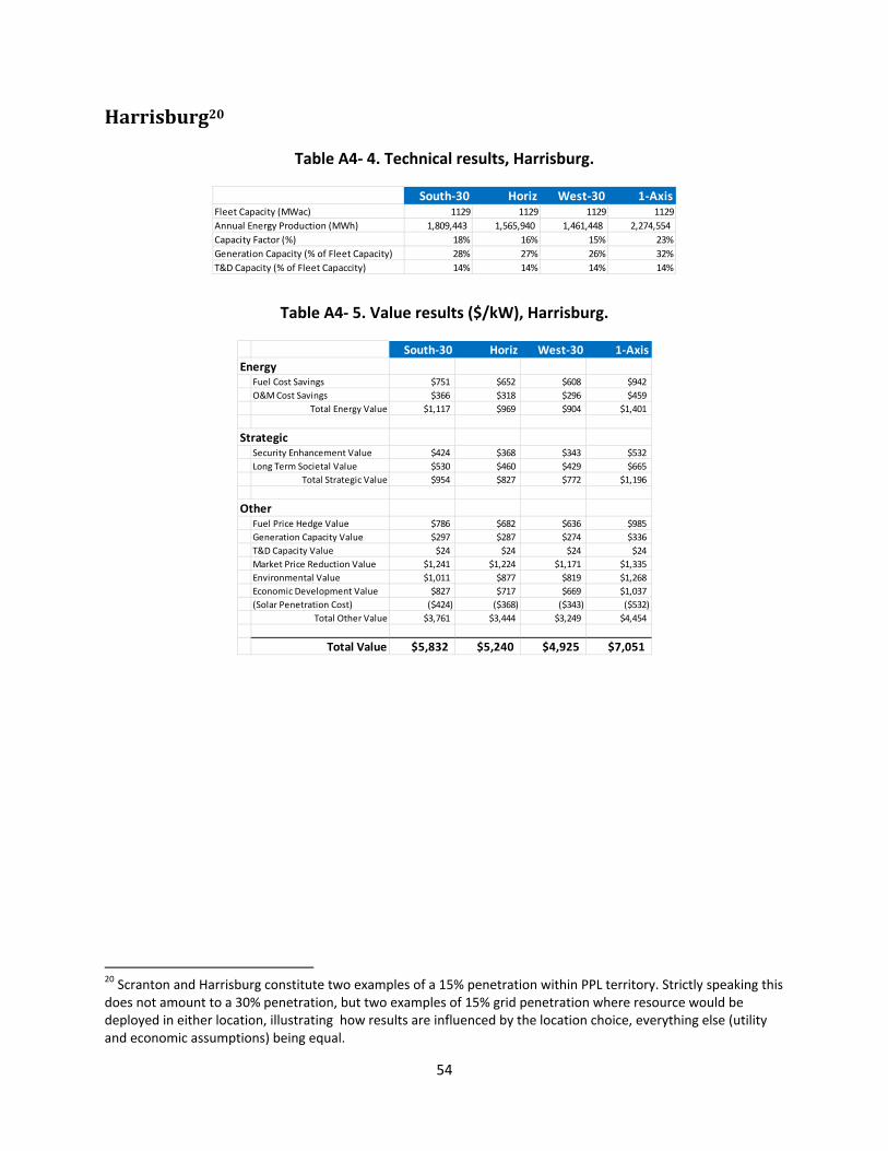
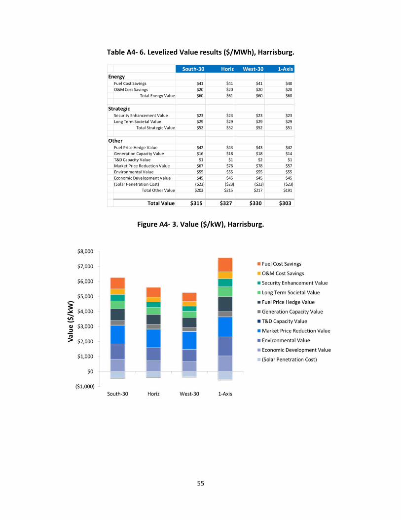
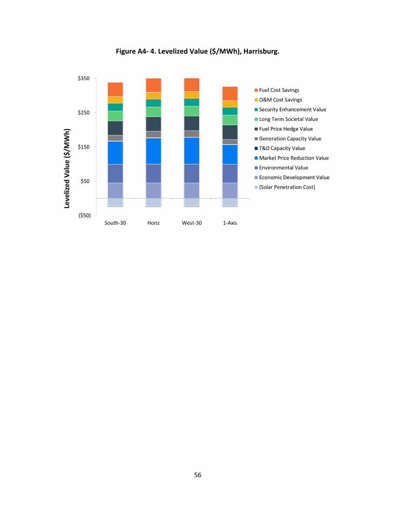
Harrisburg20

Table A4‐ 4. Technical results, Harrisburg.

Table A4‐ 5. Value results ($/kW), Harrisburg.

20 Scranton and Harrisburg constitute two examples of a 15% penetration within PPL territory. Strictly speaking this does not amount to a 30% penetration, but two examples of 15% grid penetration where resource would be deployed in either location, illustrating how results are influenced by the location choice, everything else (utility and economic assumptions) being equal.


Annual Energy Production (MWh) 1,809,443 1,565,940 1,461,448 2,274,554






O&M Cost Savings $366 $318 $296 $459

Total Energy Value $1,117 $969 $904 $1,401



Total Strategic Value $954 $827 $772 $1,196




Market Price Reduction Value $1,241 $1,224 $1,171 $1,335

Environmental Value $1,011 $877 $819 $1,268




Total Value $5,832 $5,240 $4,925 $7,051

55

Table A4‐ 6. Levelized Value results ($/MWh), Harrisburg.

Figure A4‐ 3. Value ($/kW), Harrisburg.
















Total Value $315 $327 $330 $303

56

Figure A4‐ 4. Levelized Value ($/MWh), Harrisburg.

57

Scranton

Table A4‐ 7. Technical results, Scranton.

Table A4‐ 8. Value ($/kW), Scranton.

Table A4‐ 9. Levelized Value ($/MWh), Scranton.








O&M Cost Savings $344 $300 $281 $429









Environmental Value $950 $829 $777 $1,185




Total Value $5,532 $5,001 $4,740 $6,676
















Total Value $318 $331 $334 $307

58

Figure A4‐ 5. Value ($/kW), Scranton.

Figure A4‐ 6. Levelized Value ($/MWh), Scranton.

59

Philadelphia

Table A4‐ 10. Technical results, Philadelphia.

Table A4‐ 11. Value results ($/kW), Philadelphia.

Table A4‐ 12. Levelized Value results ($/MWh), Philadelphia.








O&M Cost Savings $344 $294 $273 $432





OtherFuel Price Hedge Value $876 $747 $694 $1,100




Environmental Value $967 $825 $766 $1,214




Total Value $5,667 $5,086 $4,855 $6,912
















Total Value $304 $321 $330 $295

60

Figure A4‐ 7. Value ($/kW), Philadelphia.

Figure A4‐ 8. Levelized Value ($/MWh), Philadelphia.

61

Jamesburg

Table A4‐ 13. Technical results, Jamesburg.

Table A4‐ 14. Value results ($/kW), Jamesburg.

Table A4‐ 15. Levelized Value results ($/MWh), Jamesburg.







EnergyFuel Cost Savings $1,020 $878 $808 $1,276

O&M Cost Savings $497 $428 $394 $622




Total Strategic Value $1,234 $1,062 $978 $1,544






Economic Development Value $1,097 $944 $870 $1,373



Total Value $6,202 $5,653 $5,393 $7,492
















Total Value $257 $274 $284 $247

62

Figure A4‐ 9. Value ($/kW), Jamesburg.

Figure A4‐ 10. Levelized Value ($/MWh), Jamesburg.

63

Newark

Table A4‐ 16. Technical results, Newark.

Table A4‐ 17. Value results ($/kW), Newark.

Table A4‐ 18. Levelized Value results ($/MWh), Newark.








O&M Cost Savings $345 $298 $275 $431













Total Value $5,117 $4,685 $4,486 $6,170
















Total Value $280 $298 $310 $270

64

Figure A4‐ 11. Value ($/kW), Newark.

Figure A4‐ 12. Levelized Value ($/MWh), Newark.

65

AtlanticCity

Table A4‐ 19. Technical results, Atlantic City.

Table A4‐ 20. Value results ($/kW), Atlantic City.

Table A4‐ 21. Levelized Value results ($/MWh), Atlantic City.


Annual Energy Production (MWh) 827,924 705,374 654,811 1,039,217





EnergyFuel Cost Savings $1,081 $927 $863 $1,354

O&M Cost Savings $527 $452 $421 $660




Total Strategic Value $1,314 $1,127 $1,048 $1,646






Economic Development Value $1,168 $1,002 $932 $1,463



Total Value $6,704 $6,125 $5,929 $8,119
















Total Value $256 $274 $286 $247

66

Figure A4‐ 13. Value ($/kW), Atlantic City.

Figure A4‐ 14. Levelized Value ($/MWh), Atlantic City.

Date post:	03-Feb-2022
Category:	Documents
Upload:	others
View:	1 times
Download:	0 times