39
The Vector Space Model LBSC 708A/CMSC 838L Session 3, September 18, 2001 Douglas W. Oard
| Date post: | 01-Jan-2016 |
| Category: |
Documents |
| Upload: | georgina-stafford |
| View: | 214 times |
| Download: | 1 times |

The Vector Space Model
LBSC 708A/CMSC 838L
Session 3, September 18, 2001
Douglas W. Oard
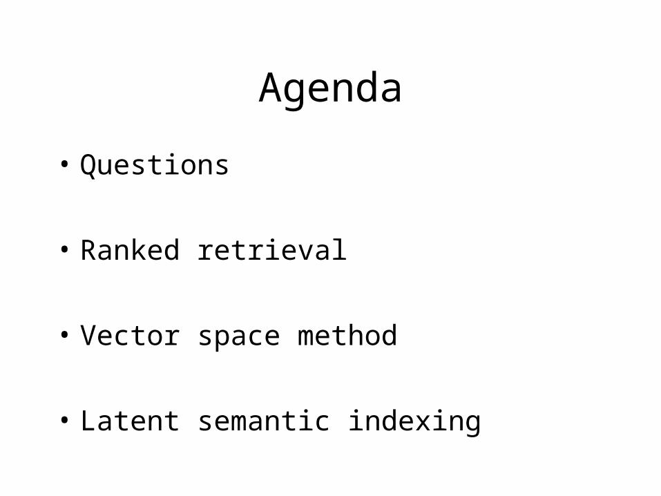
Agenda
• Questions
• Ranked retrieval
• Vector space method
• Latent semantic indexing

Strong Points of Boolean Retrieval
• Accurate, if you know the right strategy
• Efficient for the computer
• More concise than natural language
• Easy to understand
• A standard approach
• Works across languages (controlled vocab.)

Weak Points of Boolean Retrieval
• Words can have many meanings (free text)
• Hard to choose the right words– Must be familiar with the field
• Users must learn Boolean logic
• Can find relationships that don’t exist
• Sometimes find too many documents– (and sometimes get none)
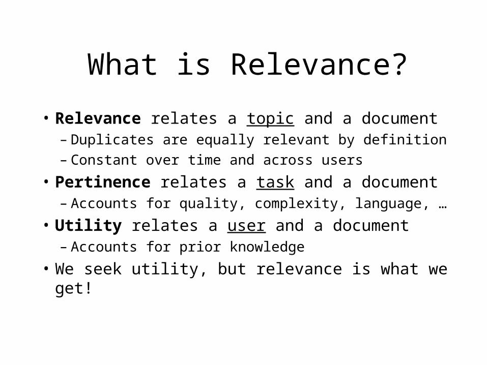
What is Relevance?
• Relevance relates a topic and a document– Duplicates are equally relevant by definition
– Constant over time and across users
• Pertinence relates a task and a document– Accounts for quality, complexity, language, …
• Utility relates a user and a document– Accounts for prior knowledge
• We seek utility, but relevance is what we get!
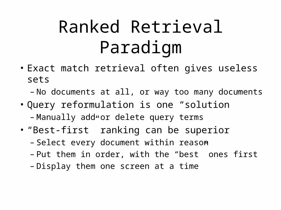
Ranked Retrieval Paradigm
• Exact match retrieval often gives useless sets– No documents at all, or way too many documents
• Query reformulation is one “solution”– Manually add or delete query terms
• “Best-first” ranking can be superior– Select every document within reason– Put them in order, with the “best” ones first– Display them one screen at a time
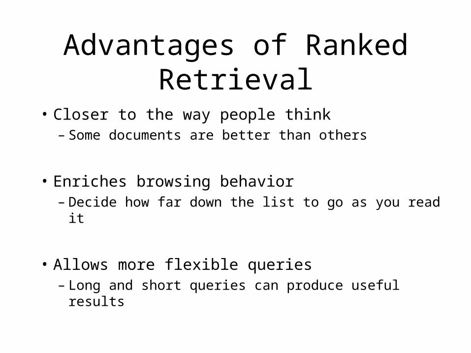
Advantages of Ranked Retrieval
• Closer to the way people think– Some documents are better than others
• Enriches browsing behavior– Decide how far down the list to go as you read it
• Allows more flexible queries– Long and short queries can produce useful results
Ranked Retrieval Challenges
• “Best first” is easy to say but hard to do!– Probabilistic retrieval tries to approximate it
• How can the user understand the ranking?– It is hard to use a tool that you don’t understand
• Efficiency may become a concern– More complex computations take more time
Partial-Match Ranking
• Form several result sets from one long query– Query for the first set is the AND of all the terms– Then all but the 1st term, all but the 2nd, …– Then all but the first two terms, …– And so on until each single term query is tried
• Remove duplicates from subsequent sets
• Display the sets in the order they were made– Document rank within a set is arbitrary

Partial Match Exampleinformation AND retrieval
Readings in Information RetrievalInformation Storage and RetrievalSpeech-Based Information Retrieval for Digital LibrariesWord Sense Disambiguation and Information Retrieval
information NOT retrieval
The State of the Art in Information Filtering
Inference Networks for Document RetrievalContent-Based Image Retrieval SystemsVideo Parsing, Retrieval and BrowsingAn Approach to Conceptual Text Retrieval Using the EuroWordNet …Cross-Language Retrieval: English/Russian/French
retrieval NOT information
Similarity-Based Queries
• Treat the query as if it were a document– Create a query bag-of-words
• Find the similarity of each document– Using the coordination measure, for example
• Rank order the documents by similarity– Most similar to the query first
• Surprisingly, this works pretty well!– Especially for very short queries

Document Similarity
• How similar are two documents?– In particular, how similar is their bag of words?
1
1
1
1: Nuclear fallout contaminated Montana.
2: Information retrieval is interesting.
3: Information retrieval is complicated.
1
1
1
1
1
1
nuclear
fallout
siberia
contaminated
interesting
complicated
information
retrieval
1
1 2 3

The Coordination Measure
• Count the number of terms in common– Based on Boolean bag-of-words
• Documents 2 and 3 share two common terms– But documents 1 and 2 share no terms at all
• Useful for “more like this” queries– “more like doc 2” would rank doc 3 ahead of doc 1
• Where have you seen this before?

Coordination Measure Example
1
1
1
1
1
1
1
1
1
nuclear
fallout
siberia
contaminated
interesting
complicated
information
retrieval
1
1 2 3
Query: complicated retrievalResult: 3, 2
Query: information retrievalResult: 2, 3
Query: interesting nuclear falloutResult: 1, 2
Term Frequency
• Terms tell us about documents– If “rabbit” appears a lot, it may be about rabbits
• Documents tell us about terms– “the” is in every document -- not discriminating
• Documents are most likely described well by rare terms that occur in them frequently– Higher “term frequency” is stronger evidence– Low “collection frequency” makes it stronger still
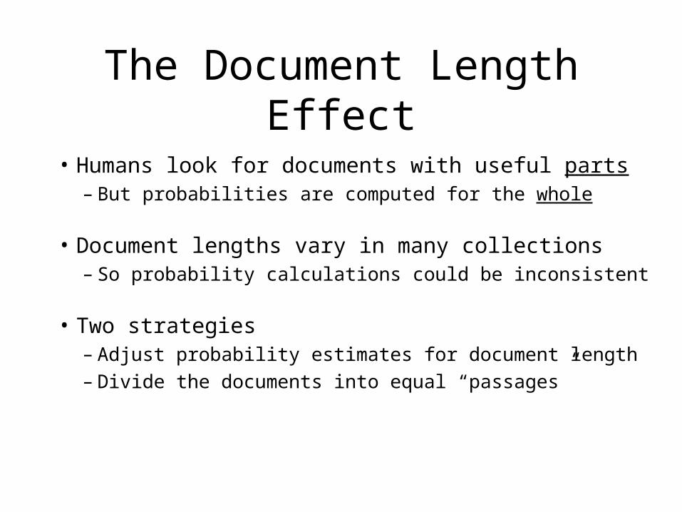
The Document Length Effect
• Humans look for documents with useful parts– But probabilities are computed for the whole
• Document lengths vary in many collections– So probability calculations could be inconsistent
• Two strategies– Adjust probability estimates for document length– Divide the documents into equal “passages”

Computing Term Contributions• “Okapi BM25 weights” are the best known
– Discovered mostly through trial and error
Let be the number of documents in the collection
Let be the number of documents containing term
Let be the frequency of term in document
Let be the contribution of term to the relevance of document
Then
N
n t
t d
w t d
w
Nn
N
t
t d
t d
t dt
tf
.. tf
tf . .length(d)
avglen
log.
log
,
,
,
t,d
t,d
0 4
0 6
05 15
0 5
1
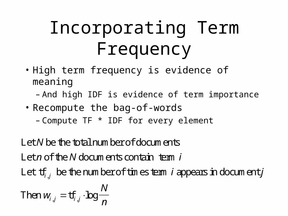
Incorporating Term Frequency
• High term frequency is evidence of meaning– And high IDF is evidence of term importance
• Recompute the bag-of-words– Compute TF * IDF for every element
Let be the total number of documents
Let of the documents contain term
Let be the number of times term appears in document
Then
N
n N i
i j
wN
n
i j
i j i j
tf
tf log
,
, ,

Weighted Matching Schemes
• Unweighted queries– Add up the weights for every matching term
• User specified query term weights– For each term, multiply the query and doc weights– Then add up those values
• Automatically computed query term weights– Most queries lack useful TF, but IDF may be useful– Used just like user-specified query term weights

TF*IDF Example
4
5
6
3
1
3
1
6
5
3
4
3
7
1
nuclear
fallout
siberia
contaminated
interesting
complicated
information
retrieval
2
1 2 3
2
3
2
4
4
0.50
0.63
0.90
0.13
0.60
0.75
1.51
0.38
0.50
2.11
0.13
1.20
1 2 3
0.60
0.38
0.50
4
0.301
0.125
0.125
0.125
0.602
0.301
0.000
0.602
idfi Unweighted query: contaminated retrievalResult: 2, 3, 1, 4
Weighted query: contaminated(3) retrieval(1)Result: 1, 3, 2, 4
IDF-weighted query: contaminated retrievalResult: 2, 3, 1, 4
tf ,i jwi j,
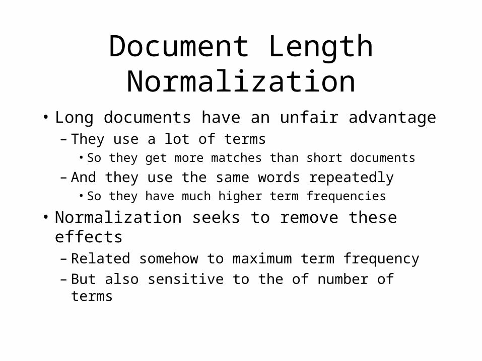
Document Length Normalization
• Long documents have an unfair advantage– They use a lot of terms
• So they get more matches than short documents
– And they use the same words repeatedly• So they have much higher term frequencies
• Normalization seeks to remove these effects– Related somehow to maximum term frequency– But also sensitive to the of number of terms
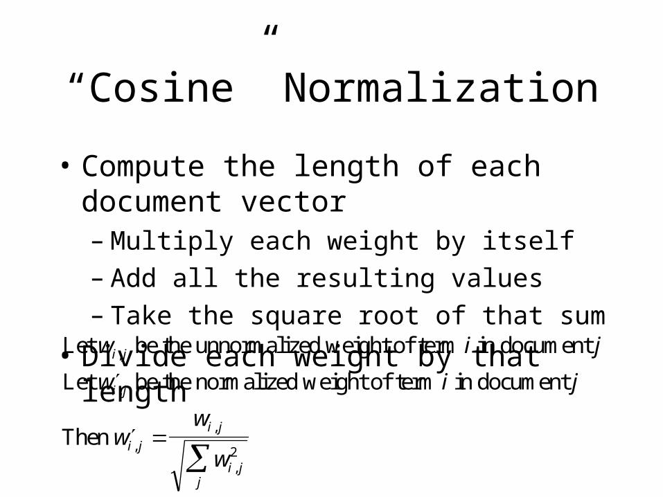
“Cosine” Normalization
• Compute the length of each document vector– Multiply each weight by itself– Add all the resulting values– Take the square root of that sum
• Divide each weight by that lengthLet be the unnormalized weight of term in document
Let be the normalized weight of term in document
Then
w i j
w i j
ww
w
i j
i j
i j
i j
i jj
,
,
,
,
,
2
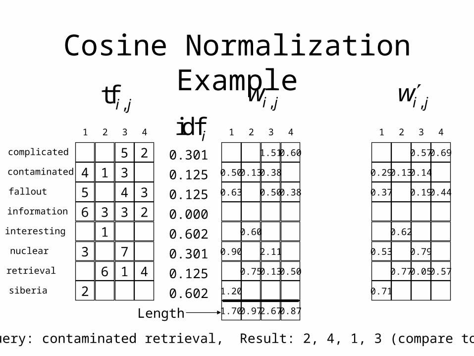
Cosine Normalization Example
0.29
0.37
0.53
0.13
0.62
0.77
0.57
0.14
0.19
0.79
0.05
0.71
1 2 3
0.69
0.44
0.57
4
4
5
6
3
1
3
1
6
5
3
4
3
7
1
nuclear
fallout
siberia
contaminated
interesting
complicated
information
retrieval
2
1 2 3
2
3
2
4
4
0.50
0.63
0.90
0.13
0.60
0.75
1.51
0.38
0.50
2.11
0.13
1.20
1 2 3
0.60
0.38
0.50
4
0.301
0.125
0.125
0.125
0.602
0.301
0.000
0.602
idfi
1.70 0.97 2.67 0.87Length
tf ,i jwi j, wi j,
Unweighted query: contaminated retrieval, Result: 2, 4, 1, 3 (compare to 2, 3, 1, 4)

Why Call It “Cosine”?
d2
d1 w j1,
w j2,
w2 2,
w2 1,
w1 1,w1 2,
Let document 1 have unit length with coordinates and
Let document 2 have unit length with coordinates and
Then
w w
w w
w w w w
1 1 2 1
1 2 2 2
1 1 1 2 2 1 2 2
, ,
, ,
, , , ,cos ( ) ( )

Interpreting the Cosine Measure
• Think of a document as a vector from zero
• Similarity is the angle between two vectors– Small angle = very similar– Large angle = little similarity
• Passes some key sanity checks– Depends on pattern of word use but not on length– Every document is most similar to itself
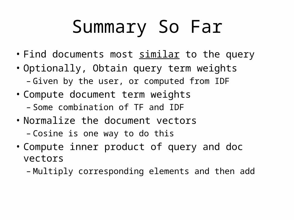
Summary So Far
• Find documents most similar to the query
• Optionally, Obtain query term weights– Given by the user, or computed from IDF
• Compute document term weights– Some combination of TF and IDF
• Normalize the document vectors– Cosine is one way to do this
• Compute inner product of query and doc vectors– Multiply corresponding elements and then add
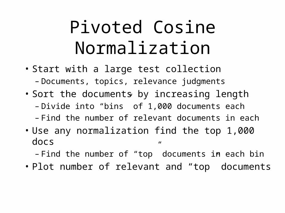
Pivoted Cosine Normalization
• Start with a large test collection– Documents, topics, relevance judgments
• Sort the documents by increasing length– Divide into “bins” of 1,000 documents each
– Find the number of relevant documents in each
• Use any normalization find the top 1,000 docs– Find the number of “top” documents in each bin
• Plot number of relevant and “top” documents
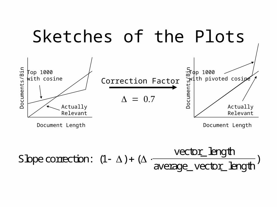
Sketches of the PlotsD
ocum
ents
/Bin Top 1000
with cosine
ActuallyRelevant
Document Length
Doc
umen
ts/B
in Top 1000with pivoted cosine
ActuallyRelevant
Document Length
Correction Factor
Slope correction: vector_ length
average_ vector_ length( ) ( )1

Pivoted Unique Normalization
• Pivoting exacerbates the cosine plot’s “tail”– Very long documents get an unfair advantage
• Coordination matching lacks such a tail– The number of unique terms grows smoothly– But pivoting is even more important (
Let be the number of unique terms in document j
tf
tf
t
wt t
j
i j
i j
ii j
j jj
,
,
,
log( )
log(avg( ))
(( ) avg( )) ( )
1
1
1
Passage Retrieval
• Another approach to long-document problem– Break it up into coherent units
• Recognizing topic boundaries is hard– But overlapping 300 word passages work fine
• Document rank is best passage rank– And passage information can help guide browsing

Stemming
• Suffix removal can improve performance– In English, word roots often precede modifiers
– Roots often convey topicality better
• Boolean systems often allow truncation– limit? -> limit, limits, limited, limitation, …
• Stemming does automatic truncation• More complex algorithms can find true roots
– But better retrieval performance does not result

Porter Stemmer
• Nine step process, 1 to 21 rules per step– Within each step, only the first valid rule fires
• Rules rewrite suffixes. Example:static RuleList step1a_rules[] = {
101, "sses", "ss", 3, 1, -1, NULL, 102, "ies", "i", 2, 0, -1, NULL, 103, "ss", "ss", 1, 1, -1, NULL, 104, "s", LAMBDA, 0, -1, -1, NULL, 000, NULL, NULL, 0, 0, 0, NULL,
};

Latent Semantic Indexing
• Term vectors can reveal term dependence– Look at the matrix as a “bag of documents”
– Compute term similarities using cosine measure
• Reduce the number of dimensions– Assign similar terms to a single composite
– Map the composite term to a single dimension
• This can be done automatically– But the optimal technique muddles the dimensions
• Terms appear anywhere in the space, not just on an axis
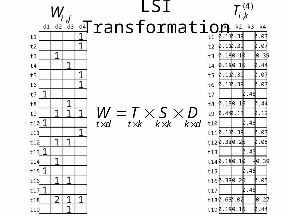
LSI Transformationd1 d2 d3 d4
12 1 1
11 1
11
11 1
11
1 1 11
111
11
11
k1 k2 k3 k4
0.15 -0.16 0.44
0.63 0.02 -0.27
0.45
0.33 -0.26 0.05
0.45
0.18 -0.10 -0.39
0.45
0.33 -0.26 0.05
0.11 0.39 0.07
0.45
0.44 0.13 0.12
0.15 -0.16 0.44
0.45
0.11 0.39 0.07
0.11 0.39 0.07
0.44
0.18 -0.10 -0.39
0.11 0.39 0.07
0.11 0.39 0.07
0.15 -0.16
t1
t2
t3
t4
t5
t6
t7
t8
t9
t10
t11
t12
t13
t14
t15
t16
t17
t18
t19
t1
t2
t3
t4
t5
t6
t7
t8
t9
t10
t11
t12
t13
t14
t15
t16
t17
t18
t19
Wi j, Ti k,( )4
W T S Dt d t k k k k d
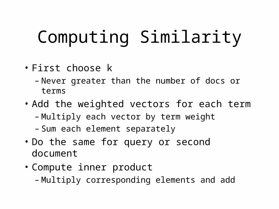
Computing Similarity
• First choose k – Never greater than the number of docs or terms
• Add the weighted vectors for each term– Multiply each vector by term weight
– Sum each element separately
• Do the same for query or second document• Compute inner product
– Multiply corresponding elements and add

LSI Exampled2 d3
12 1
1 1
1
1 1
1 11
11
k1 k2 k3 k4
0.15 -0.16 0.44
0.63 0.02 -0.27
0.33 -0.26 0.05
0.18 -0.10 -0.39
0.33 -0.26 0.05
0.44 0.13 0.12
0.15 -0.16 0.44
0.44
0.18 -0.10 -0.39
0.15 -0.16
t1
t2
t3
t4
t5
t6
t7
t8
t9
t10
t11
t12
t13
t14
t15
t16
t17
t18
t19
t3
t4
t8
t9
t12
t14
t16
t18
t19
Wi j,
0.44 0.13 0.12t9
0.33 -0.26 0.05t12
0.33 -0.26 0.05t16
0.63 0.02 -0.27t18
k1 k2 k3 k4
0.63 0.02 -0.27t18
2.72 -0.55 -1.10Sum2
2.18 -0.85 1.26Sum3
d d2 3 5 00 .
Sum Sum .2 3 501
Removing Dimensionsk1 and k2 = 6.40k1 alone = 5.92

Benefits of LSI
• Removing dimensions can improve things– Assigns similar vectors to similar terms
• Queries and new documents easily added– “Folding in” as weighted sum of term vectors
• Gets the same cosines with shorter vectors

Weaknesses of LSI
• Words with several meanings confound LSI– Places them at the midpoint of the right positions
• LSI vectors are dense– Sparse vectors (tf*idf) have several advantages
• The required computations are expensive– But T matrix and doc vectors are done in advance– Query vector and cosine at query time
• The cosine may not be the best measure– Pivoted normalization can probably help

Two Minute Paper
• Vector space retrieval finds documents that are “similar” to the query. Why is this a reasonable thing to do?
• What was the muddiest point in today’s lecture?


