WORKING PAPER SERIES NO 1675 / MAY 2014 THE VIX, THE VARIANCE PREMIUM AND STOCK MARKET VOLATILITY Geert Bekaert and Marie Hoerova In 2014 all ECB publications feature a motif taken from the €20 banknote. NOTE: This Working Paper should not be reported as representing the views of the European Central Bank (ECB). The views expressed are those of the authors and do not necessarily reflect those of the ECB.
Transcript
Work ing PaPer Ser ieSno 1675 / May 2014
The ViX, The Variance PreMiuMand STock MarkeT VolaTiliTy
Geert Bekaert and Marie Hoerova
In 2014 all ECB publications
feature a motif taken from
the €20 banknote.
noTe: This Working Paper should not be reported as representing the views of the European Central Bank (ECB). The views expressed are those of the authors and do not necessarily reflect those of the ECB.
ISSN 1725-2806 (online)EU Catalogue No QB-AR-14-049-EN-N (online)
Any reproduction, publication and reprint in the form of a different publication, whether printed or produced electronically, in whole or in part, is permitted only with the explicit written authorisation of the ECB or the authors.This paper can be downloaded without charge from http://www.ecb.europa.eu or from the Social Science Research Network electronic library at http://ssrn.com/abstract_id=2252209.Information on all of the papers published in the ECB Working Paper Series can be found on the ECB’s website, http://www.ecb.europa.eu/pub/scientific/wps/date/html/index.en.html
AcknowledgementsWe thank the Editor, Alok Bhargava, and three anonymous reviewers for useful comments and suggestions that improved the paper. Carlos Garcia de Andoain provided excellent research assistance. Geert Bekaert acknowledges financial support from Netspar. The views expressed do not necessarily reflect those of the European Central Bank or the Eurosystem.
Geert BekaertColumbia University
Marie Hoerova (corresponding author)European Central Bank; e-mail: [email protected]
1
Abstract
We decompose the squared VIX index, derived from US S&P500 options prices, into
the conditional variance of stock returns and the equity variance premium. We evaluate a
plethora of state-of-the-art volatility forecasting models to produce an accurate measure
of the conditional variance. We then examine the predictive power of the VIX and its two
components for stock market returns, economic activity and financial instability. The
variance premium predicts stock returns while the conditional stock market variance
predicts economic activity and has a relatively higher predictive power for financial
The 2007-2009 crisis has intensified the need for indicators of the risk aversion of
market participants. It has also become increasingly commonplace to assume that
changes in risk appetites are an important determinant of asset prices. Not surprisingly,
the behavioral finance literature (see e.g. Baker and Wurgler, 2007) has developed
“sentiment indices,” and financial institutions have created a wide variety of “risk
aversion” indicators (see Coudert and Gex (2008) for a survey).
One simple candidate indicator is the equity variance premium, the difference
between the squared VIX index and an estimate of the conditional variance of the stock
market. The VIX index is the “risk-neutral” expected stock market variance for the US
S&P500 contract and is computed from a panel of options prices. Well-known as a “fear
index” (Whaley, 2000) for asset markets, it reflects both stock market uncertainty (the
“physical” expected volatility), and a variance risk premium, which is also the expected
premium from selling stock market variance in a swap contract. Bollerslev, Tauchen and
Zhou (2009) show that an estimate of this variance premium predicts stock returns;
Bekaert, Hoerova, and Lo Duca (2013) show that there are strong interactions between
monetary policy and the variance premium, suggesting that monetary policy may actually
affect risk aversion in the market place. The variance premium uses objective financial
market information and naturally “cleanses” option-implied volatility from the effect of
physical volatility dynamics and uncertainty, leaving a measure correlated with risk
aversion.
How to measure the variance premium is not without controversy however,
because it relies on an estimate of the conditional variance of stock returns. In this article,
we tackle several measurement issues for the variance premium, assessing a plethora of
state-of-the-art volatility models and making full use of overlapping daily data, rather
than sparse end-of-month data, which is standard.
The conditional variance measure is of interest in its own right. First, there is a
long literature on the trade-off between risk, as measured by the conditional variance of
stock market returns, and the aggregate risk premium on the market (see e.g. French,
Schwert and Stambaugh (1987) for a seminal contribution). This long line of research has
mostly failed to uncover a strong positive relationship between risk and return (see Bali,
3
2008, for a summary). Second, stock market volatility can also be viewed as a market-
based measure of economic uncertainty. For example, Bloom (2009) shows that
heightened “economic uncertainty” decreases employment and output. Interestingly, he
uses the VIX index to measure uncertainty, so that his results may actually be driven by
the variance premium rather than uncertainty per se.
Using more plausible estimates of the variance premium and stock market
volatility, we then assess whether they predict stock returns, economic activity, as well as
financial instability, an economic outcome that has garnered considerable policy interest
in the aftermath of the recent financial crisis. We find that the equity variance risk
premium predicts stock returns while stock market volatility mostly does not. By
contrast, stock market volatility predicts industrial production growth, a measure of
economic activity, while equity variance premium has no predictive power for future
economic activity. Moreover, conditional variance predicts financial instability more
strongly than does the variance premium, especially at longer horizons.
4
1. Introduction
The 2007-2009 crisis has intensified the need for indicators of the risk aversion of
market participants. It has also become increasingly commonplace to assume that
changes in risk appetites are an important determinant of asset prices. Not surprisingly,
the behavioral finance literature (see e.g. Baker and Wurgler, 2007) has developed
“sentiment indices,” and financial institutions have created a wide variety of “risk
aversion” indicators (see Coudert and Gex (2008) for a survey).
One simple candidate indicator is the equity variance premium, the difference
between the squared VIX index and an estimate of the conditional variance of the stock
market. The VIX index is the “risk-neutral” expected stock market variance for the US
S&P500 contract and is computed from a panel of options prices. Well-known as a “fear
index” (Whaley, 2000) for asset markets, it reflects both stock market uncertainty (the
“physical” expected volatility), and a variance risk premium, which is also the expected
premium from selling stock market variance in a swap contract. Bollerslev, Tauchen and
Zhou (2009) show that an estimate of this variance premium predicts stock returns;
Bekaert, Hoerova, and Lo Duca (2013) show that there are strong interactions between
monetary policy and the variance premium, suggesting that monetary policy may actually
affect risk aversion in the market place. The variance premium uses objective financial
market information and naturally “cleanses” option-implied volatility from the effect of
physical volatility dynamics and uncertainty, leaving a measure correlated with risk
aversion.
How to measure the variance premium is not without controversy however, because it
relies on an estimate of the conditional variance of stock returns. For example, the
measure proposed in Bollerslev, Tauchen and Zhou (2009), BTZ, henceforth, assumes
that the conditional variance of stock market returns is a martingale, an assumption which
is not supported by the data, leading to potentially biased variance premiums. In this
paper, we tackle several measurement issues for the variance premium, assessing a
plethora of state-of-the-art volatility models and making full use of overlapping daily
data, rather than sparse end-of-month data, which is standard.
The conditional variance measure is of interest in its own right. First, there is a long
literature on the trade-off between risk, as measured by the conditional variance of stock
5
market returns, and the aggregate risk premium on the market (see e.g. French, Schwert
and Stambaugh (1987) for a seminal contribution). This long line of research has mostly
failed to uncover a strong positive relationship between risk and return (see Bali, 2008,
for a summary). Second, stock market volatility can also be viewed as a market-based
measure of economic uncertainty. For example, Bloom (2009) shows that heightened
“economic uncertainty” decreases employment and output. Interestingly, he uses the VIX
index to measure uncertainty, so that his results may actually be driven by the variance
premium rather than uncertainty per se.
Using more plausible estimates of the variance premium and stock market volatility,
we then assess whether they predict stock returns, economic activity, as well as financial
instability, an economic outcome that has garnered considerable policy interest in the
aftermath of the recent financial crisis. We find that the well-known results in BTZ
exaggerate the predictive power of the variance premium for stock returns. However, the
equity variance risk premium remains a reliable predictor of stock returns. Stock market
volatility does not predict the stock market, but it is a much better predictor of economic
activity than is the equity variance premium. It also predicts financial instability more
strongly than does the variance premium, especially at longer horizons.
The remainder of the paper is organized as follows. Section 2 discusses the
econometric framework that we use to forecast volatility, and lays out our model
selection procedure. Section 3 reports the results of our specification analysis and
forecasting performance comparison. Section 4 uses the preferred estimates of the
variance premium and stock market volatility to predict stock returns, economic activity
and financial instability. Section 5 concludes.
2. Econometric Framework
We define the variance risk premium as:
)22(
1
2
tttt RVEVIXVP (1)
Here the VIX is the implied option volatility of the S&P500 index for contracts with a
maturity of one month, and )22(
1tRV is the S&P500 realized variance measured over the
next month (22 trading days) using 5 minute returns. Note that 2)22(
1 tt VIXRV is the
return to buying variance in a variance swap contract. Therefore, technically speaking,
6
the variance risk premium refers to the negative of VP. Since that number is mostly
negative, we prefer to define it as we did in equation (1).
Economically, the squared VIX is the conditional return variance using a “risk-
neutral” probability measure, whereas the conditional variance uses the actual “physical”
probability measure. The risk-adjusted measure shifts probability mass to states with
higher marginal utility (bad states) and this implies that in many realistic economic
settings, the variance premium will be increasing in the economy’s risk aversion.
The unconditional mean of the variance premium is easy to compute by simply
computing the average of )22(
1
2
tt RVVIX . However, we are interested in the conditional
variance premium as described in equation (1), which relies on the physical conditional
expected value of the future realized variance. The common approach to estimate this
uses empirical projections of the realized variance on variables in the information set, and
subtracts this estimated expected variance from the 2VIX to arrive at VP. Hence, the
problem is reduced to one of variance forecasting.
Our data start on January 02, 1990 (the start of the model-free VIX series)2 and covers
the period until October 01, 2010. We have a total of 5208 daily, overlapping
observations. The recent crisis period presents special challenges as stock market
volatilities peaked at unprecedented levels, but at the same time the crisis represents an
informative period during which uncertainty and risk aversion may have been particularly
pronounced. Nevertheless, if we decompose the sample variance of the VIX time series in
contributions by crisis and non-crisis observations, the former dominate despite
representing a relatively small part of the sample. We deal with these challenges by
considering both models that predict the level and the logarithm of realized variances,
and by putting much emphasis on parameter stability in our model selection procedure. In
addition, we focus on out-of-sample forecasting exercises where we conduct the in-
sample estimations mostly on non-crisis observations, so that the influence of the crisis
on the parameter estimates and model selection is mitigated.
2 The CBOE changed the methodology for calculating the VIX, initially measuring implied volatility for the S&P100 index, to be measured in a model–free manner from a panel of option prices (see Bakshi, Madan and Kapadia, 2003, for details) only in September 2003. It then backdated the new model–free index to 1990 using historical option prices.
7
Variance forecasting
There is an extensive econometric literature on volatility forecasting. It is now
generally accepted that models based on high frequency realized variances dominate
standard models in the GARCH class (see e.g. Chen and Ghysels, 2012) and we therefore
examine the state-of-the-art models in that class. These models stress the importance of
persistence (using lagged realized variances as predictors), additional information content
in the most recent return variances (Corsi, 2009), asymmetry between positive and
negative return shocks (the classic volatility asymmetry, see e.g. Engle and Ng, 1993) and
potentially differing predictive information present in jump versus continuous volatility
components (Andersen, Bollerslev, and Diebold, 2007). We accommodate all of these
elements in our model.
In the finance literature, it has been pointed out as early as in Christensen and
Prabhala (1998) that option prices as reflected in implied volatility should have
information about future stock market volatility. This motivates using the VIX as a
predictive variable. Recent articles using the VIX in similar forecasting exercises include
Busch, Christensen and Nielsen (2011) who examine a number of variance forecasting
models embedding option-implied volatility for bond, currency and stock markets, and
Andersen and Bondarenko (2007) who mostly focus on measurement issues with the
officially published VIX index. Of course, because the VIX also embeds a risk premium, it
will not be an unbiased predictor of future realized volatility. Chernov (2007) argues that
spot volatility is likely to have additional information about future volatility.
Finally, it is well-known that estimation noise hurts out-of-sample forecasting
performance. Simple models such as the martingale model may therefore outperform
more complex models. We therefore also consider a number of non-estimated models that
are special cases of our general framework.
Our most general forecasting model can be represented as follows:
ttd
tw
tm
td
tw
tm
td
tw
tm
tt
rrr
JJJCCCVIXcRV
)1(22
)5(22
)22(22
)1(22
)5(22
)22(22
)1(22
)5(22
)22(22
222
)22(
(2)
We want to forecast the monthly (22 trading days) S&P500 realized variance, denoted by
)22(
tRV , and defined as the sum of daily realized variances RV over the 22 days,
returns and the squared close-to-open return, with returns expressed in percentage form.3
Our first independent variable is the VIX 2 (expressed in monthly percentages squared, i.e.
VIX2/12 where VIX is the quoted VIX index level in annualized percent), and we expect
to be positive. The next six variables separate the realized variance into a continuous
and a discontinuous (“jump”) component (at the monthly, weekly and daily frequencies),
following Andersen, Bollerslev and Diebold (2007). To isolate the jumps contribution to
daily quadratic variation, we use threshold bipower variation proposed by Corsi, Pirino
and Renò (2010). Corsi et al. (2010) show that this threshold measure substantially
reduces the small-sample bias that the standard bipower variation (Barndorff-Nielsen and
Shephard, 2004) estimates exhibit.4 The daily jump, denoted as tJ , is defined as:
0,max ttt TBPVRVJ (3)
where TBPVt stands for threshold bipower variation defined in Corsi et al. (2010),
equation (2.14). The continuous component of the daily quadratic variation is given by:
ttt JRVC (4)
Weekly (h=5) and monthly (h=22) variables are averaged, and we express all variables in
monthly units so that:
h
jjt
ht J
hJ
11
)( 22 and
h
jjt
ht C
hC
11
)( 22 .
Finally, following Corsi and Renò (2012), we add negative returns over the past day,
week and month, to incorporate a potential leverage effect (see Campbell and Hentschel,
1992; Bekaert and Wu, 2000). To model the leverage effect at different frequencies, we
define 0,min )()( ht
ht rr where
h
jjt
ht r
hr
11
)( 22 .
In addition to forecasting realized variance in levels, we also consider models that
predict the logarithm of the realized variance. The logarithmic counterpart of the model
3 We use actual S&P500 returns. Other papers in the literature focused on S&P500 futures including, e.g., Andersen, Bollerslev and Diebold (2007) and Corsi, Pirino and Renò (2010). 4 The upward bias in bipower variation leads to a continuous variation that is too large and a jump component that is too small, and thus potentially also biases estimates of the jumps coefficients in models such as (2). To obtain threshold bipower variation, we use equation (2.14) in Corsi et al. (2010), with the threshold function as defined in their equation (2.15) and the scale-free constant set to 3. The construction of the estimator of the local variance is described in Appendix B of their paper.
9
in (2) reads:
t
)(t
d)(t
w)(t
m)(t
d)(t
w
)(t
m)(t
d)(t
w)(t
mt
)(t
εrδrδrδJγJγ
JγCβCβCβVIXαcRV
122
522
2222
122
522
2222
122
522
2222
222
22
1ln1ln
1lnlnlnlnlnln (5)
Because variances have right-skewed distributions, but logarithmic variances tend to have
near Gaussian distributions, it may be easier to predict logarithmic variances with linear
models. However, ultimately, we still need to identify the model that best forecasts the
level of the realized variance. To this end, when we consider a logarithmic model, we
assume log-normality to predict levels of monthly realized variances:
)22(
1
)22(
1
)22(
1 var2
1exp ttttt rvrvERVE (6)
where )22(
1
)22(
1 ln tt RVrv . We use the logarithmic model to compute the conditional
expectation of )22(
1trv and the sample variance of )22(
1trv to compute the variance term.
Model selection procedure
Our model selection procedure consists of comparing the out-of-sample forecasting
performance of a set of 31 estimated and non-estimated models and examining their
stability. The models are summarized in Table 1. For estimated models, we consider 14
variants of the encompassing model in levels (equation (2)) and in logarithms (equation
(5)), respectively. We estimate the models using OLS. Models 1 through 13 have fixed
combinations of predictors. Models 14 for the level and the logarithmic specification,
respectively, are models with a set of predictors selected by a general-to-specific (Gets)
model selection procedure (using the full sample). While sequential Wald tests present
problems in terms of selecting the size of tests (see e.g. Bhargava, 1987), we rely on the
large body of work on model selection by David Hendry and co-authors, see e.g.
Campos, Hendry and Krolzig (2003) and Hendry and Krolzig (2005). We use the recent
implementation by Autometrics in the econometrics software package OxMetrics (see
Doornik, 2009, for details) Thus, we estimate 28 models in total. In terms of practical
implementation, we use 5% as the target size for our tests, the default value in the
software; we also do not use indicator saturation techniques, but test for parameter
instability separately. We use PcGive, version 13 (see Doornik and Hendry, 2009).
In Table 2, we discuss the level and logarithmic models chosen by the Gets- model
selection analysis. The standard errors below the parameters are computed using 44
10
Newey-West (1987) lags. The model selection yields models with monthly, weekly and
daily continuous variation in both cases. In the level regression model, the general-to-
specific model selection procedure retains monthly jumps, in addition to negative returns
at all three frequencies. In the logarithmic model, the squared VIX is chosen, along with
the daily negative returns.
In addition, we consider 3 non-estimated models: the lagged squared VIX (model 29);
the lagged realized variance (model 30; this is the model used in BTZ); and 0.5 times the
lagged squared VIX plus 0.5 times the lagged realized variance (model 31).
We estimate the models using daily data between January 1, 1990 and July 15, 2005
(representing about 75% of the full sample) and use the rest of the sample (till October
01, 2010) to measure forecasting performance. The parameters are not updated.
We examine five different criteria. We compute the root-mean-squared error
(RMSE), mean absolute error (MAE), and mean absolute percentage error (MAPE; the
absolute error in percent of the actual realized variance). We evaluate whether the
forecast error measures are significantly different among competing forecasting models
through the Diebold and Mariano (1995) test (with standard errors computed using 44
Newey-West lags), using a 10% significance level. We also compute the R2 of Mincer–
Zarnowitz (1969) forecasting regressions, that is, we compute the R2 in a regression of
actual data on their forecasted values.5 The final criterion we examine is a simple joint
Chow test for parameter stability over the last part of the sample versus the estimation
part of the sample. Ericksson (1992) discusses formally how mean-squared-error
minimization and parameter constancy are both necessary (but not sufficient) conditions
to obtain a good forecasting model. We also produce the average correlation of the
forecasts produced by a particular model with the forecasts produced by the winning
model on each of the first 4 criteria. This gives a sense of how close different forecast
models are economically.
5 We also computed two other statistics; the heteroskedasticity adjusted root-mean-squared error suggested in Bollerslev and Ghysels (1996) and the QLIKE loss function (see Patton, 2011). However, these statistics produce rankings very similar to the MAPE-criterion, so we do not discuss them further. Also note that the Diebold and Mariano test only uses the forecast errors and ignores the underlying model structure and estimation. While we could in principle use more complex statistics that take the model structure and estimation into account (see e.g. West, 2006), recent research suggests that the Diebold and Mariano test works well even in model-based out-of-sample forecasting comparisons (see Clark and McCracken, 2011; Diebold, 2013).
11
3. Model Selection Results
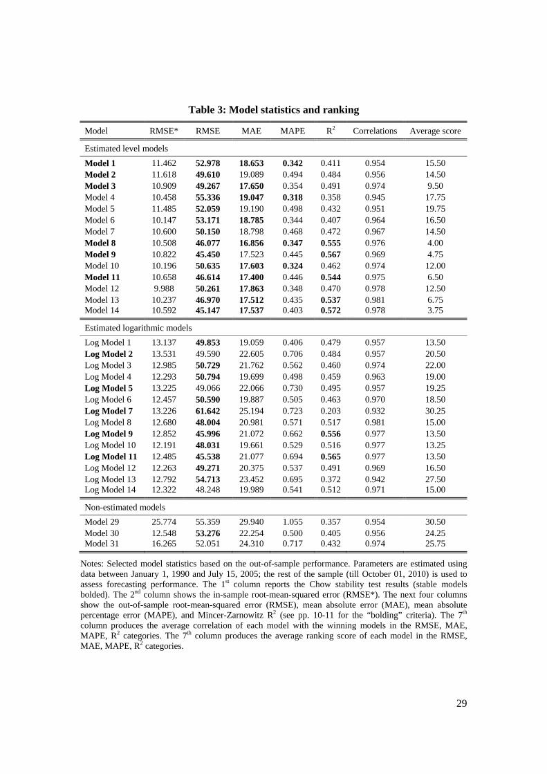
Table 3 produces the statistics and the average ranking of our 31 considered models
according to the criteria discussed above. Recall that for the logarithmic models, we are
predicting the level of the realized variance as discussed in Section 2. The first column
reports whether the model is stable according to the Chow test (using 10% significance
level). Stable models are bolded. In the second column, we report the in-sample RMSE
(denoted RMSE*). In the next three columns, we report the out-of-sample RMSE, MAE
and MAPE criteria.6 We note that the out-of-sample RMSE is considerably larger than its
in-sample counterpart. This is also true for the MAE criterion, but it is not true for the
MAPE criterion, where out-of-sample errors are often smaller than in-sample errors (not
reported). Because the realized variance became very large during the crisis, which
constitutes a substantial part of the out sample, it is not surprising to see larger (absolute)
errors out of sample. However, the results for the MAPE criterion suggest that, in relative
terms, the errors did not increase. We test for each model whether it generates a statistic
significantly different from the statistic generated by the best ranked model (i.e., model
14 for RMSE, model 8 for MAE, and model 4 for MAPE; all models in levels). When
such a test fails to reject, the statistic is bolded. We view such tests as critical in model
selection. A model may rank relatively low, but the criterion may have little power to
distinguish different models and generate very similar forecast errors. For example, a
quick glance at the table reveals that the RMSE criterion has little power to distinguish
alternative models, while MAPE is the most distinguishing one. For the R2 criterion (in
the 5th column), we view a difference of more than 5% with the winning model (model
14) as a significant difference in economic terms. Model statistics similar in R2 to the
winning model are bolded. The 6th column produces an average correlation, averaging the
correlation of each model’s forecasts with the forecasts of the winning models in all four
out-of-sample quantitative criteria (RMSE, MAE, MAPE, and R2). If a model were to be
the top model on each criterion, it would get a correlation of 1. Finally, we rank models
in each of the four categories (from 1, best, to 31, worst) and produce the average ranking
score for each model in the last column of Table 3.
6 Although the Diebold-Mariano test uses the mean-squared error (MSE) rather than RMSE, we report the RMSE so that RMSE and MAE criteria have a comparable scale (both are in the realized variance units, monthly percentages squared). MAPE is expressed in percent of the realized variance and is thus scale-free.
12
Using this information, we winnow down our set of models by requiring a good
model to be bolded in at least 3 out of 4 quantitative criteria. This leaves us with only 7
models: level models 1, 4, 8, 10, 11, 13 and 14. Model 14 produces the best average
ranking score (3.75) but is not stable. Indeed, only three of these seven models are stable:
models 1, 8 and 11. Model 8 has the second best average score (4). It is also the only
model which gets four bolds. Model 11 has the fourth best average score (6.5).
Meanwhile, model 1 ranks only 16 in the average score. We therefore select models 8 and
11 as the winning models. Model 8 is Corsi’s HAR model, supplemented with the
squared VIX. Model 11 features continuous and jump variations at all three frequencies.
More generally, the presence of realized variances (or their continuous components) at all
three frequencies is important in delivering lower error statistics. In terms of R2, more
complex models (level models 8, 9, 11, 13, 14 and logarithmic models 9 and 11) yield
substantially higher values than the other models.
Over the full sample, the resulting coefficients for models 8 and 11 (with
heteroskedasticity-robust standard errors in brackets) are:
026.0117.0096.0072.0903.1
107.0330.0199.0108.0730.3 )1(22
)5(22
)22(22
222
)22( ttttt RVRVRVVIXRV
(7)
056.0262.0702.0064.0064.0237.0164.1
016.0327.0742.1223.0237.0212.0855.3 )1(22
)5(22
)22(22
)1(22
)5(22
)22(22
)22( ttttttt JJJCCCRV (8)
Table 3 also shows statistics of some popular simple models used in the literature: the
squared VIX – realized variance model used in Bekaert, Hoerova, Lo Duca (2013) (our
model 3), the martingale model of BTZ (model 30) and the AR(1) model of Londono
(2011) (model 2). Compared to the top models, the martingale and simple autoregressive
models perform an order of magnitude worse but the squared VIX – realized variance
model delivers quite similar performance. Of the simpler models, Model 3 is best on all
four criteria (only Model 1 does better on MAPE). It also has the best average score
among the simpler models, and the sixth best average score overall.
Additional exercises
We performed two alternative exercises. First, we repeated our analysis with two
alternative sample splits in the out-of-sample forecasting exercise. We estimated the
models using data until June 16, 2003 (about 65% of the full sample) and until August 1,
13
2007 (about 85% of the sample), respectively. Results for the winning models 8 and 11
are remarkably robust. For the 65% split, out-of-sample forecasting performance is
uniformly better, with lower errors and higher R2, with the best model attaining an R2 of
just over 59%, i.e., 2% higher than in the 75% split. The winning models are the same as
in the 75% split: model 4 on MAPE, model 8 on MAE, and model 14 on R2 and RMSE.
Models that get 3 bolds out of 4 are models 1, 3, 4, 8, 10, and 14 (all in levels), with
models 4, 10 and 14 being unstable (as in the 75% sample split). Model 8 is again the
only model that gets 4 bolds. For the 85% split, where all out-of-sample predictions are
made over the period that includes the recent financial crisis, all models produce higher
errors and lower R2. Model 8 is again the winning model on the MAE criterion, with
level model 10 winning on MAPE and logarithmic model 11 on RMSE and R2. Models
that get 3 bolds out of 4 largely overlap with those in the 75% split: models 4, 8, 9, 10,
11, 13 and 14. Only models 8, 9 and 11 are stable, however. In sum, model 8 is
consistently a top performer across all three sample splits. Model 11 does well in two of
three sample splits, including the split that emphasizes performance during the financial
crisis.7
Second, we re-consider our forecasting exercise with end-of-month data. In most of
the existing articles (including BTZ, Londono, 2011, and Busch, Christensen and
Nielsen, 2011), end-of-month data are used to estimate conditional variance models. The
use of daily data should lead to more efficient estimates, but the correlation between daily
and monthly data induced by the overlapping data structure may make the increase in
efficiency minor. We estimated all our models using end-of-the-month data till mid-2005,
mimicking the 75% sample split used in our main forecasting exercise with daily data.
We then use the obtained regression coefficients to construct daily out-of-sample realized
variance forecasts for the remainder of the sample. Computing the usual criteria, we
check whether we can accept the various models by looking for three bolds on our four
quantitative criteria (MAPE, MAE, RMSE, and R2), and we verify the stability criterion.
7 We also verified that our winning models are overall stable. That is, using the monthly data set we conducted the standard unknown breakpoint test (Quandt-Andrews test; implemented in EViews 6), with 10% trimming, and found no evidence of instability. The test points to June 2008 as the most likely break for both models 8 and 11 but it is not statistically significant.
14
With end-of-month data, the winning models in the four quantitative categories are
the same as with the daily data (Model 4 on MAPE, Model 8 on MAE, and Model 14 on
RMSE and R2). The winning models based on daily data beat those based on monthly
data on all statistics with the exception of the MAPE criterion, where model 4 displays
very comparable statistics (0.317 with end-of-month versus 0.318 with daily data).
Models 1, 4 and 8 still get 3 bolds out of 4. However, model 4 is again unstable.
Interestingly, model 8 based on monthly estimates does well relative to the best models
based on the daily information. When estimated using the full sample, the monthly model
puts less weight on the squared VIX and RV(22), and more weight on RV(5) and RV(1) than
the daily model does. For the simpler models, model 3 (used in Bekaert, Hoerova, Lo
Duca, 2013) and model 1 are stable, and get 3 bolds out of 4. However, model 3 does
better on all four quantitative criteria than model 1. The more complex models, like our
previously winning model 11, which include jumps and/or asymmetric volatility, are, not
surprisingly, more difficult to identify with monthly data. The use of monthly estimation
samples should therefore best be restricted to relatively simple models, where the loss of
efficiency is not very costly.
4. Economics and Predictability
Risk and risk aversion
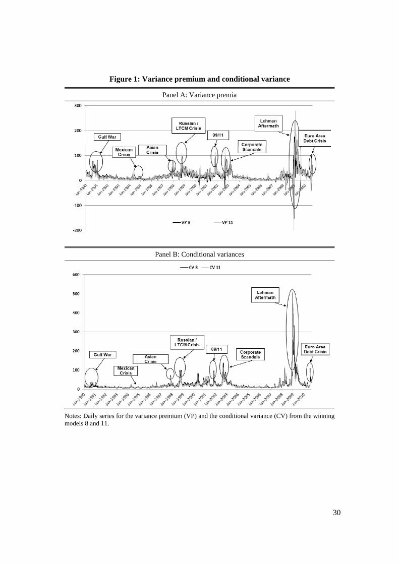
In Figure 1, we plot the daily series for the variance risk premium (VP henceforth;
displayed in Panel A), which may potentially serve as a proxy for risk aversion, and the
conditional (physical) variance of the stock market (CV henceforth; in Panel B), which
may potentially serve as a measure of economic uncertainty. We show the two series
obtained from the winning models 8 and 11 on one graph. The VP and CV series are
positively correlated (correlation of 0.45 for model 8 and 0.27 for model 11) and display
peaks at the expected times. The largest peaks for CV are observed during the Lehman
aftermath in the recent crisis and at the time of the corporate scandals following the
Enron debacle. Interestingly, the 1998 Russian crisis and the Gulf war did not generate
much uncertainty, but these events do feature substantially elevated levels of VP. The
Lehman event seems to have caused both massive uncertainty and massive risk aversion.
When realized variances show extreme peaks, the VP series can become negative,
15
which happens more for model 11 than for model 8. This is a disadvantage of all these
models. It is unlikely that during these periods of stress, there was a sudden increase in
risk appetite. The more mundane explanation is that realized variances likely have
different components with different levels of mean reversion. In a massive crisis, some of
the realized variance movements should probably be allowed to mean-revert more
quickly and not affect the conditional variance as much as they do now. The models with
jumps could theoretically capture this by having negative coefficients on the jump terms.
However, model 11 puts a large positive coefficient on the monthly and weekly jump
components, and a very small negative one on the daily jump component. Overall, it is
likely that a non-linear model may be better equipped to capture the behavior of CV and
VP in severe crises.
Predicting stock market returns
The two components of the squared VIX index have been considered as separate
potential predictors of stock market returns. Starting with French, Schwert and
Stambaugh (1987), a large literature focuses on the relationship between aggregate stock
market returns and their conditional variance. In a simple static CAPM model, the
coefficient on the conditional stock market variance would be the wealth weighted risk
aversion coefficient, but such a relationship need not hold perfectly in a dynamic model.
In the literature on the risk–return relationship, estimates vary from positive to negative
and the relationship is often insignificant. Lundblad (2007) suggests that the samples
typically used are too short to uncover a relationship that is robustly and statistically
significantly positive in the sample of over 150 years that he considers. Yet, the
measurement of the conditional variance of stock returns may matter too. The bulk of the
extant literature has considered GARCH-in-mean models to measure the conditional
stock market variance, which likely induces substantial measurement error in the
regression. Ghysels, Santa Clara and Valkanov (2005) recover a positive risk-return
trade-off measuring the conditional variance with a flexible function of past returns,
applying MIDAS modeling. However, Hedegaard and Hodrick (2013) dispute these
results, mostly finding insignificant coefficients with either GARCH or (adjusted)
MIDAS models to measure the conditional variance.
BTZ recently showed that the variance risk premium has predictive power for future
16
stock returns, which is logical since it harbors information about aggregate risk aversion.
As shown above, their measure implicitly uses a volatility model that is strongly rejected
by the data. We therefore reconsider the predictive power of both the equity variance risk
premium (“risk”) and the conditional variance of the stock market (“uncertainty”), using
our improved measures of the conditional variance of stock market returns.
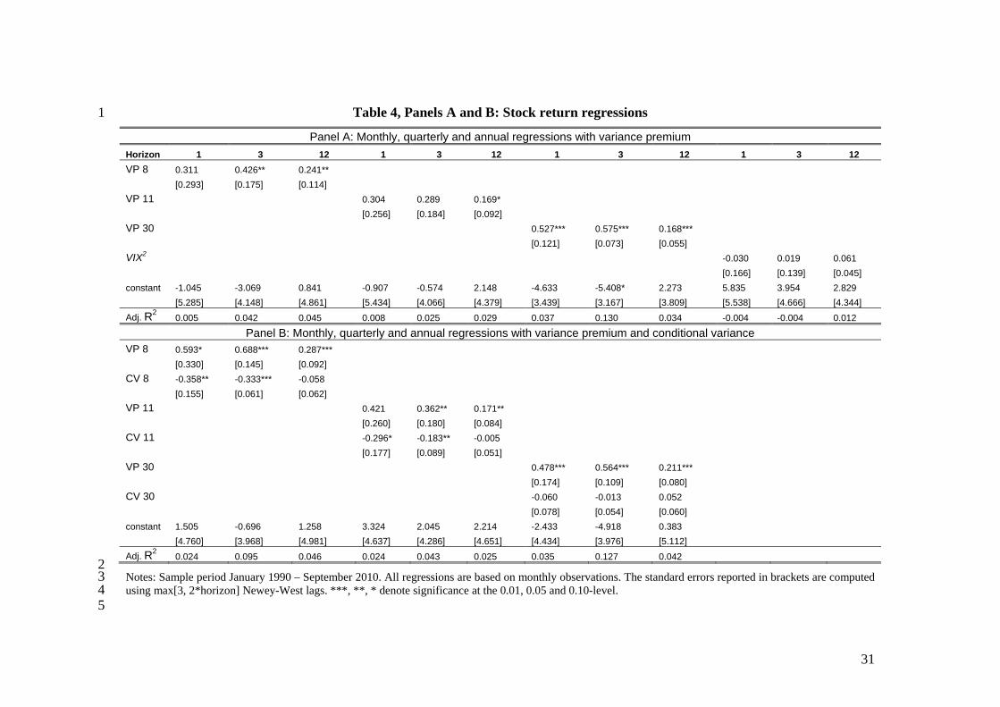
We start with regressions using only the variance premium as a predictor of equity
returns. Like BTZ, we rely on end-of-the-month observations but we consider various
estimates of the variance premium.8 Table 4, Panel A contains the results. The left hand
side variable is always excess stock returns (the S&P500 return in excess of the three-
month T-bill rate; expressed in annualized percentages). We use three different horizons,
monthly, quarterly and annual (denoted by 1, 3 and 12, respectively), averaging returns
over a quarter/year. The overlap in the monthly data creates serial correlation in the error
term that must be corrected for in creating standard errors. We use a relatively large
number of Newey-West lags, namely max{3, 2*horizon}, to do so, rather than create
standard errors under the null of no predictability, as in Hodrick (1992). While the
Hodrick estimator has very good size properties, selecting a large number of lags may
improve power (see Sun, Phillips, and Jin, 2008).
In the last specification in Panel A, we show that the squared VIX itself fails to predict
stock returns. Just above, we repeat the BTZ specification that uses the past realized
variance as the estimate of the conditional variance of stock market returns. The resulting
variance premium proxy predicts stock market returns at all three horizons with the
predictive power strongest at the quarterly horizon, both in terms of magnitude of the
coefficient and the adjusted R2. The R2 for the martingale model in the quarterly
regression increases from 7% in the original BTZ sample to 13% in our sample. Thus,
including the financial crisis actually strengthens BTZ’s results. Compared to the
predictability results when using the two best models - models 8 and 11 - to estimate the
variance premium, BTZ’s martingale model maximizes the predictive power of the
variance premium for returns. For the best models, there is only statistically significant
predictive power at the longer horizons and the R2 drops from 13% to somewhere
8 We also performed all of our regressions using the BTZ sample, which ends in December 2007 and therefore conveniently excludes the crisis period. We mention any interesting differences between results with and without the crisis period.
17
between 2 and 4.5%.9 In unreported results, we find that the realized variance predicts
stock returns with a negative sign at the monthly and quarterly horizon (significant at the
10% and 5% level, respectively). However, the coefficients are an order of magnitude
smaller than for the BTZ variance premium, and the R2 is just above 2% in the quarterly
regression.
This generates somewhat of a puzzle regarding the origin of the strong predictive
power of the BTZ-variance premium. If the realized variance is not a strong predictor of
stock market returns and the VIX itself does not predict them at all, why does their
difference provide strong predictive power? The coefficient on the variance premium can
be decomposed as follows:
VP
RV
VP
VIXCVVIXVP var
var
var
var 2
2 (9)
It turns out that the variance of the squared VIX is rather similar to the variance of RV,
which is itself more than three times higher than the variance of the variance risk
premium. Therefore, the variance premium coefficient at the quarterly frequency scales
up the small positive coefficient on the VIX and the larger negative coefficient on stock
market volatility by a factor of three.10
Economically, it does appear that the variance risk premium uncovers a component in
the VIX index that is related to future stock market returns, but the statistical evidence is
not very strong. Apart from the small sample, one possible reason for this is the well-
known fact that equity risk premiums are likely driven by multiple state variables (see
Ang and Bekaert; 2007, Menzly, Santos and Veronesi, 2004) so that the univariate
regressions are necessarily mis-specified. In the consumption-based asset pricing model
of Bekaert, Engstrom and Xing (2009), risk aversion and uncertainty are the two state
variables driving time-variation in the equity risk premium.11
We therefore investigate bivariate regressions using both the variance premium and 9 One possibility is that because we pre-estimate the conditional variance and BTZ do not, measurement noise affects our estimates. However, our measurement provides proxies for the variance premium and the conditional stock market variance closer to the true economic concepts. 10 In the BTZ sample, neither the squared VIX nor the realized variance predict stock returns, with the VIX getting a positive insignificant coefficient and the realized variance a zero coefficient in the quarterly regressions. In that sample, the variance of the squared VIX is more than twice as high as the variance of the BTZ variance risk premium so that the positive coefficient on the VIX gets scaled up by a factor of two. 11 Anderson, Ghysels, and Juergens (2009) also examine the impact of “risk” and “uncertainty”, but in their paper risk represents physical volatility and uncertainty disagreement among forecasters.
18
the conditional variance as predictors. The results are in Panel B of Table 4. The VP is
overall the stronger predictor over the quarterly and annual horizons. The CV coefficients
are (with one exception) negative and sometimes significantly so for models 8 and 11.12
These results have implications for the consumption–based asset pricing literature,
where there is a persistent debate about what economic mechanism generates a large
equity premium, volatile stock market returns and long–horizon stock return
predictability. In the Bansal–Yaron (2004) long-run risk model, time–variation in the
equity premium comes from time–variation in economic uncertainty. Recent versions of
the model (see e.g. Bansal, Kiku, Yaron, 2012) put more and more emphasis on the role
of volatility and argue that substantial persistence in consumption volatility (which then
generates high persistence in stock return volatility) is necessary to make the models fit
the salient asset return features. However, our empirical results cast doubt on this
economic mechanism. The persistence of the conditional variance (at the monthly level)
is modest, varying between 0.63 and 0.71 across models. Moreover, the time-varying risk
premium component in equity returns comes predominantly from the variance risk
premium, not from time-varying economic uncertainty. The effects of economic
uncertainty on risk premiums we do document seem short-lived. This suggests that the
alternative class of models (see Campbell and Cochrane, 1999), which relies on counter-
cyclical changes in risk aversion to generate variation in risk premiums, has more chance
of being the true economic mechanism explaining time-variation in equity risk premiums.
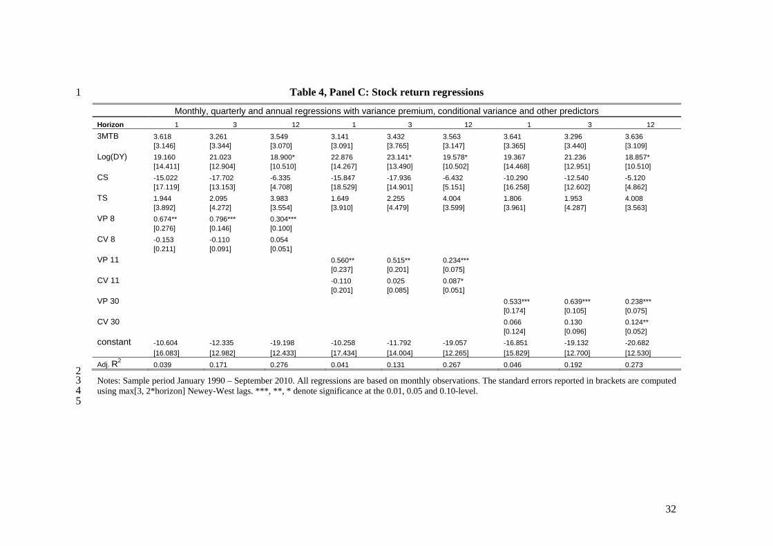
In Panel C, we consider a multivariate regression including other well-known
predictor-variables, namely the real 3-month rate (the three-month T-bill minus CPI
inflation, denoted 3MTB), the logarithm of the dividend yield (denoted Log(DY)), the
credit spread (the difference between Moody’s BAA and AAA bond yield indices,
denoted CS) and the term spread (the difference between the 10-year and the 3-month
Treasury yields, denoted TS); all variables expressed in annualized percentages. The
addition of the other variables strengthens the predictive power of the variance premium
for equity returns, with the coefficients uniformly increasing. However, the uncertainty
coefficients are now smaller and mostly insignificantly different from zero.
12 In the BTZ sample, the CV coefficients are positive at the monthly, and negative at the quarterly and annual horizons, but mostly insignificant.
19
As to the other variables, the term structure variables are never significant. Both the
real rate and the term spread have consistently positive coefficients. The credit spread
obtains a negative coefficient that is not significantly different from zero, and the
dividend yield is at best significant at the 10% level, mostly at the longer horizons. Here,
the crisis adversely affected the predictive power of these variables. Excluding crisis data,
the dividend yield and the credit spread are highly statistically significantly different from
zero for all specifications (at all horizons in case of the dividend yield and at longer
horizons in case of the credit spread), with the dividend yield having the expected
positive coefficient, but the credit spread negatively affecting the equity premium.13
The adjusted R2’s remains small at the one month horizon, but now becomes quite
large at the quarterly (13 to 19% range) and annual horizons (around 27%). It is likely
that this high explanatory power may partially reflect statistical bias (see Boudoukh,
Richardson and Whitelaw, 2007).
Given that our preferred VP and CV measures are based on the estimated models 8
and 11, we conduct a robustness check which accounts for the sampling error in the VP
and CV in our regressions. Specifically, we draw 500 alternative VP and CV series from
the distribution of VP and CV estimates. To do so, we retain the coefficients from the
forecasting projection together with their asymptotic covariance matrix. Then, we draw
500 alternative parameter coefficients from the distribution of these estimates, generating
alternative VP and CV estimates. We then feed these into our predictive regressions
generating a distribution of coefficients, standard errors and t-statistics. As the first-stage
projections are tightly estimated, the coefficients and standard errors are not materially
affected, and our main inference regarding stock return predictability remains intact.
Predicting the Real Economy and Financial Instability
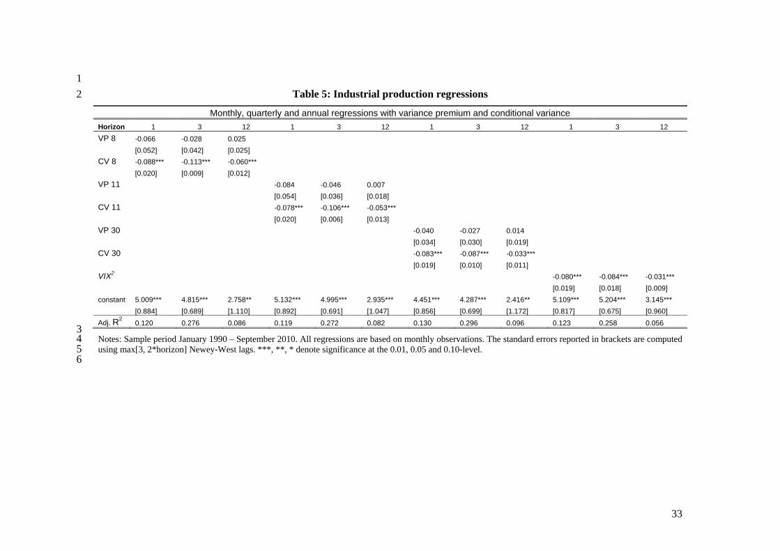
In Table 5, we examine the predictive power of the variance risk premium and stock
market volatility for economic activity as measured by industrial production growth (the
13 There is no issue of multi-collinearity in the regression as the dividend yield–credit spread correlation is low (close to zero over the pre-crisis sample; and 0.2 over the full sample). While the negative credit spread coefficient may surprise some readers, BTZ also report negative coefficients for the credit spread in univariate excess return regressions. It is conceivable that the credit spread is a good indicator of economic prospects (for example, it is relatively highly correlated with economic uncertainty) and therefore helps cleanse the dividend yield from variation driven by cash flows, rather than risk premiums (see Golez, 2012 for a recent interesting attempt to cleanse the dividend yield of cash flow effects in a predictability regression).
20
log-difference of the total industrial production index expressed in annualized
percentages; growth over a quarter/year is averaged). Bloom (2009) shows that
uncertainty shocks lead to a rapid drop and rebound in aggregate output and employment.
In a model with adjustment costs to labour and capital, this occurs because higher
uncertainty causes firms to temporarily pause their investment and hiring. In some of his
empirical work, Bloom actually uses the VIX to help measure uncertainty shocks. Here,
we investigate whether the VIX and/or its two components predict economic activity in a
simple regression framework.
The last specification shows that the squared VIX itself predicts economic activity
with a negative sign at all horizons (significant at the 1% level). In terms of economic
significance, a 1% (monthly) move in the VIX near the mean leads approximately to a 1%
(annualized) drop in the industrial production growth over the next quarter. The bivariate
regressions with its two components show that whatever predictive power the VIX has for
future output, is coming from the uncertainty component. The coefficient on VP is
negative at monthly and quarterly horizons, but it is always statistically insignificantly
different from zero. The coefficient on CV is always negative and statistically significant
at the 1% level for all three horizons. As with stock return regressions, we check
robustness of our results to accounting for the sampling error in the VP and CV estimates.
Our results are unaltered. We conclude that CV is a robust and significant predictor of
economic activity.
Our results here add to a rapidly growing literature on predicting economic activity
with economic uncertainty measures. For example, Stock and Watson (2012) argue that
financial disruptions and heightened uncertainty helped produce the Great Recession.
Allen, Bali, and Tang (2012) derive a measure of aggregate systemic risk using data on
stock returns for banks and show that high levels of this measure predict future economic
downturns. Bachmann, Elstner and Sims (2013) use survey expectations data to construct
an empirical proxy for time-varying business-level uncertainty. They show that surprise
movements in the uncertainty proxy lead to significant reductions in production. Finally,
Gilchrist, Sim, and Zakrajsek (2010) analyze how fluctuations in uncertainty interact with
financial market imperfections in determining economic outcomes.
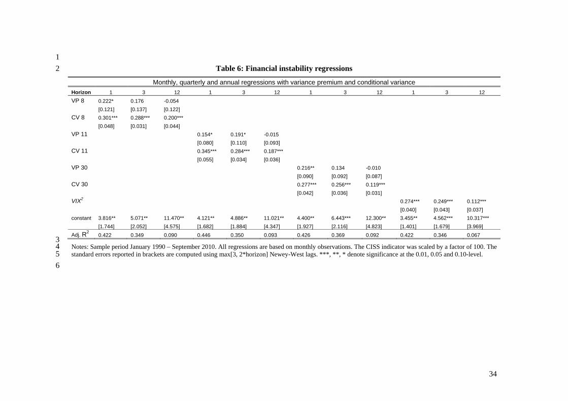
One economic outcome that has garnered considerable policy interest since the recent
21
global crisis is financial instability. In Table 6, we examine whether measures of the
variance risk premium and stock market volatility have predictive power for financial
instability. To measure financial instability, we use a financial stress indicator created by
the European Central Bank (called CISS). The indicator is based on European Monetary
Union (EMU) data, combining information from the money, equity, bond, and foreign
exchange markets, and some financial intermediaries-related information. It mostly
comprises realized volatilities for various return, currency or interest rate measures and it
does not contain any implied volatility information (see Hollo, Kremer and Lo Duca,
2012, for details). We regress the level of the CISS indicator 1, 3 and 12 months ahead on
our VP and CV measures.
The VIX itself has a high predictive power for the one- and three-months ahead
indicators (significant at the 1% level). The R2 is over 40% at the monthly horizon and
over 30% at the quarterly horizon. When both components of the VIX enter the
regressions, the uncertainty component has a higher predictive power than the variance
premium component. Uncertainty is significant at 1% level at all three horizons, and the
magnitude of its coefficients is uniformly higher than for the VP, particularly at the
quarterly and annual horizons. The VP coefficient is significant at the monthly horizon
(at the 5-10% level) but not (with the exception of model 11) at the quarterly or annual
frequency. These results are robust to accounting for the sampling error in the VP and CV
estimates. Overall, a high predictive power of variables based on US data for a European
financial stress indicator is noteworthy.14
5. Conclusions
We decompose the squared VIX, the risk neutral expected stock market variance, into
two components, the conditional (physical) variance of the stock market (CV) and the
equity variance premium (VP), which is the difference between the two (VP=VIX2-CV).
14 We also considered three alternative financial stress indicators: a (proprietary) CISS indicator based on US data, an indicator developed by the Kansas Fed and an indicator developed by the St. Louis Fed. Results for the US CISS are very similar to those for the EMU CISS (the correlation between the two indicators is 0.8). For the Fed-developed indicators, results are similar with two qualifications. First, the coefficients on the VP component are now statistically significant at 1% level at both the monthly and quarterly frequency. This is not surprising as both indicators include the VIX itself as one of the components (unlike the CISS indicators). Second, the R2’s are higher at the monthly and quarterly frequency compared to the regressions with the EMU CISS indicator. VP and CV have a higher predictive power for financial stress in the US compared to Europe.
22
Because this decomposition critically depends on the accuracy of the model for CV, we
first conduct an extensive analysis of state-of-the-art variance forecasting models, where
we make sure to also consider the squared VIX itself as a potential predictor. Indeed, one
of our winning models includes the VIX.
We use these models to re-examine and expand the evidence on the predictive power
of VP and CV for stock returns, economic activity (as measured by industrial production)
and financial stress indicators (tracked by central banks). We find that the variance
premium is a significant predictor of stock returns, but the conditional variance mostly is
not. However, CV robustly and significantly predicts economic activity with a negative
sign, whereas VP has no predictive power for future output growth. Lastly, CV has a
relatively higher predictive power for financial instability than does the variance
premium.
23
REFERENCES
Allen, L., T.G. Bali, and Y. Tang (2012). “Does Systemic Risk in the Financial Sector Predict Future Economic Downturns?”, Review of Financial Studies 25(10), 3000-3036.
Andersen, T.G., and O. Bondarenko (2007). “Construction and Interpretation of Model-Free Implied Volatility,” in I. Nelken (Ed.), Volatility as an Asset Class, Risk Books,
London, UK (2007), 141–181.
Andersen, T. G., T. Bollerslev and F. X. Diebold (2007). “Roughing It Up: Including Jump Components in the Measurement, Modeling, and Forecasting of Return Volatility,” Review of Economics and Statistics 89(4), 701-720.
Anderson, E., E. Ghysels, and J.L. Juergens (2009). “The Impact of Risk and Uncertainty on Expected Returns,” Journal of Financial Economics, 94(2), 233-263.
Ang, A. and G. Bekaert (2007). “Stock Return Predictability: Is it There?” Review of Financial Studies, 20(3), 651-707.
Bachmann, R., S. Elstner and E. R. Sims (2013). “Uncertainty and Economic Activity: Evidence from Business Survey Data,” American Economic Journal: Macroeconomics 5(2), 217-49.
Baker, M. and J. Wurgler (2007). “Investor sentiment in the stock market,” Journal of Economic Perspectives 21(2), 129-152.
Bakshi, G., N. Kapadia and D. Madan (2003). “Stock Return Characteristics, Skew Laws, and Differential Pricing of Individual Equity Options,” Review of Financial Studies 16(1), 101-143.
Bali, T.G. (2008). “The Intertemporal Relation between Expected Returns and Risk,” Journal of Financial Economics 87(1), 101-131.
Bansal R. and A. Yaron (2004). “Risks for the Long-Run: A Potential resolution of Asset Pricing Puzzles,” Journal of Finance 59(4), 1481-1509.
Bansal R., D. Kiku and A. Yaron (2012). “An Empirical Evaluation of the Long-Run Risks Model for Asset Prices,” Critical Finance Review 1, 183-221.
Barndorff-Nielsen, O., and M. Shepherd (2004). “Power and Bi-Power Variation with Stochastic Volatility and Jumps,” Journal of Financial Econometrics 2(1), 1-37.
Bekaert, G., M. Hoerova and M. Lo Duca (2013). “Risk, Uncertainty, and Monetary Policy,” Journal of Monetary Economics 60(7), 771-788.
Bekaert, G. and E. Engstrom (2010). “Asset Return Dynamics under Bad Environment-Good Environment Fundamentals,” working paper, Columbia GSB.
Bekaert, G., E. Engstrom, and Y. Xing (2009). “Risk, Uncertainty, and Asset Prices,” Journal of Financial Economics 91, 59-82.
Bekaert, G. and G. Wu, (2000), “Asymmetric Volatility and Risk in Equity Markets,” Review of Financial Studies 13(1), 1-42.
Bhargava, A. (1987). “Wald Tests and Systems of Stochastic Equations,” International Economic Review 28(3), 789-808.
24
Bloom, N. (2009). “The Impact of Uncertainty Shocks,” Econometrica 77(3), 623-685.
Bollerslev, T. and E. Ghysels (1996). “Periodic Autoregressive Conditional Heteroscedasticity,” Journal of Business & Economic Statistics 14(2), 139-51.
Bollerslev, T., G. Tauchen and H. Zhou (2009). “Expected Stock Returns and Variance Risk Premia,” Review of Financial Studies 22(11), 4463-4492.
Boudoukh, J., M. Richardson, and R.Whitelaw (2007). “The Myth of Long-Horizon Predictability,” Review of Financial Studies 24(4), 1577-1605.
Britten-Jones, M. and A. Neuberger (2000). “Option Prices, Implied Price Processes, and Stochastic Volatility,” Journal of Finance 55(2), 839-866.
Busch, T., B.J. Christensen, and M.O. Nielsen (2011). “The role of implied volatility in forecasting future realized volatility and jumps in foreign exchange, stock, and bond markets,” Journal of Econometrics 160(1), 48-57.
Campbell, J.Y. and J. Cochrane (1999). “By Force of Habit: A Consumption Based Explanation of Aggregate Stock Market Behavior,” Journal of Political Economy 107(2), 205-251.
Campbell, J.Y. and Ludger Hentschel (1992). “No News is Good News: An Asymmetric Model of Changing Volatility in Stock Returns,” Journal of Financial Economics 31(3), 281-318.
Campos, J., D.F. Hendry, and H.M. Krolzig (2003). “Consistent Model Selection by an Automatic Gets Approach,” Oxford Bulletin of Economics and Statistics 65, 803-819.
Carr, P. and L. Wu (2009). “Variance Risk Premiums,” Review of Financial Studies 22(3), 1311-1341.
Chen, X. and E. Ghysels (2012). “News – Good or Bad – and its Impact on Volatility Predictions over Multiple Horizons,” Review of Financial Studies 24(1), 46-81.
Chernov, M (2007). “On the Role of Risk Premia in Volatility Forecasting,” Journal of Business & Economic Statistics 25(4), 411-426.
Chicago Board Options Exchange (2004). “VIX CBOE Volatility Index,” White Paper.
Christensen, B.J. and N.R. Prabhala (1998). “The Relation between Implied and Realized Volatility,” Journal of Financial Economics 50(2), 125-150.
Clark, T.E. and M.W. McCracken (2011). “Nested Forecast Model Comparisons: A New Approach to Testing Equal Accuracy,” Manuscript, Federal Reserve Banks of Cleveland and St. Louis.
Corsi F. (2009). “A Simple Approximate Long Memory Model of Realized Volatility,” Journal of Financial Econometrics 7(2), 174-196.
Corsi F. and R. Renò (2012). “Discrete-time Volatility Forecasting with Persistent Leverage Effect and the Link with Continuous-time Volatility Modeling,” Journal of Business & Economic Statistics, forthcoming.
Corsi F., D. Pirino and R. Renò (2010). “Threshold Bipower Variation and the Impact of Jumps on Volatility Forecasting,” Journal of Econometrics 159(2), 276-288.
25
Coudert, V. and M. Gex (2008). “Does Risk Aversion Drive Financial Crises? Testing the Predictive Power of Empirical Indicators,” Journal of Empirical Finance 15, 167-184.
Diebold, F. X., (2013) “Comparing Predictive Accuracy, Twenty Years Later: A Personal Perspective on the Use and Abuse of Diebold-Mariano Tests,” working paper, University of Pennsylvania.
Diebold, F. X. and R.S. Mariano (1995). “Comparing Predictive Accuracy,” Journal of Business & Economic Statistics 13(3), 253-63.
Doornik, J. A. (2009), “Autometrics,” Chapter 4 in J.L. Castle and N. Shephard (eds.) The Methodology and Practice of Econometrics: A Festschrift in Honour of David F. Hendry, Oxford University Press, Oxford, 88-121.
Doornik, J. A., and D. F. Hendry (2009). PcGive 13: Empirical Econometric Modelling Using PcGive13, Volume I, Timberlake Consultants Press, London.
Engle, R. and V. Ng (1993). “Measuring and Testing the Impact of News and Volatility,” Journal of Finance 48(5), 1749-1778.
Ericsson, N. R. (1992). “Parameter Constancy, Mean Square Forecast Errors, and Measuring Forecast Performance: An Exposition, Extensions, and Illustration,” Journal of Policy Modeling, 14(4), 465-495.
French, K., W. Schwert and R. Stambaugh (1987), “Expected Stock Returns and Volatility,” Journal of Financial Economics 19, 3-29.
Ghysels, E., P. Santa-Clara, and R. Valkanov (2005). “There is a risk-return trade-off after all,” Journal of Financial Economics 76(3), 509-548.
Gilchrist, S., J.W. Sim and E. Zakrajsek (2010). “Uncertainty, Financial Frictions, and Investment Dynamics,” working paper.
Golez, B. (2012). “Expected Returns and Dividend Growth Rates Implied in Derivative Markets,” working paper, University of Notre Dame.
Hedegaard, E. and R.J. Hodrick (2013). “Estimating the Conditional CAPM with Overlapping Data Inference,” working paper, Columbia GSB.
Hendry, D.F. and H.M. Krolzig (2005), “The Properties of Automatic Gets Modelling,” Economic Journal, 115, C32-C61.
Hodrick, R.J. (1992). “Dividend yields and expected stock returns: alternative procedures for inference and measurement”, Review of Financial Studies 5(3), 357-386.
Holló, D., M. Kremer, and M. Lo Duca (2012). “CISS - a composite indicator of systemic stress in the financial system,” ECB Working Paper No. 1426.
Londono, J.M. (2011). “The Variance Risk Premium around the World,” IFDP Working Paper.
Lundblad, C. (2007). “The Risk Return Tradeoff in the Long-Run: 1836-2003,” Journal of Financial Economics 85, 123-150.
Menzly, L., T. Santos, and P. Veronesi (2004), “Understanding Predictability”, Journal of Political Economy 112, 1-47.
26
Mincer, J. and V. Zarnowitz (1969). “The Evaluation of Economic Forecasts,” In: J.
Mincer (Ed.), Economic Forecasts and Expectations, NBER, New York, 3–46.
Newey, W. and K. West (1987). “A Simple, Positive Semi-definite, Heteroskedasticity and Autocorrelation Consistent Covariance Matrix,” Econometrica 55(3), 703-708.
Patton, A. (2011). “Volatility Forecast Comparison using Imperfect Volatility Proxies,” 2011, Journal of Econometrics 160(1), 246-256.
Stock, J.H. and M.W. Watson (2012). “Disentangling the Channels of the 2007–09 Recession,” Brookings Papers on Economic Activity, Spring 2012.
Sun, Y., P.C.B. Phillips and S. Jin (2008). “Optimal Bandwidth Selection in Heteroskedasticity-Autocorrelation Robust Testing,” Econometrica 76(1), 175-194.
West, K.D. (2006). “Forecast Evaluation,” In G. Elliott, C. Granger and A. Timmerman (eds.), Handbook of Economic Forecasting, Volume 1, Elsevier, 100-134.
Whaley, R. E. (2000). “The Investor Fear Gauge,” Journal of Portfolio Management, Spring, 12-17.
Estimated models (Log) Model 1 X (Log) Model 2 X (Log) Model 3 X X (Log) Model 4 X X X (Log) Model 5 X X (Log) Model 6 X X X X (Log) Model 7 X X X (Log) Model 8 X X X (Log) Model 9 X X (Log) Model 10 X X X X X (Log) Model 11 X X X X (Log) Model 12 X X X X X X X (Log) Model 13 X X X X X X (Log) Model 14 Outcome of the general-to-specific (Gets) model selection - see Table 2 Non-estimated models Model 29 X Model 30 X Model 31 0.5* X 0.5*X
Notes: Summary of variables included in estimated and non-estimated models. In models without jumps, the relevant realized variances (RV(22), RV(5) and RV(1)) are used instead of the continuous variations (C(22), C(5) and C(1)); i.e., in estimated (log) models 2, 3, 8, 9, and non-estimated models 30 and 31.
28
Table 2: General-to-specific (Gets) model selection
Notes: Sample period January 02, 1990 – October 01, 2010. Column 1 reports estimates for the level model while column 2 reports estimates for the logarithmic model. The standard errors reported in brackets are computed using 44 Newey-West lags. ***, **, * denote significance at the 0.01, 0.05 and 0.10-level.
29
Table 3: Model statistics and ranking
Model RMSE* RMSE MAE MAPE R2 Correlations Average score
Estimated level models
Model 1 11.462 52.978 18.653 0.342 0.411 0.954 15.50 Model 2 11.618 49.610 19.089 0.494 0.484 0.956 14.50 Model 3 10.909 49.267 17.650 0.354 0.491 0.974 9.50 Model 4 10.458 55.336 19.047 0.318 0.358 0.945 17.75 Model 5 11.485 52.059 19.190 0.498 0.432 0.951 19.75 Model 6 10.147 53.171 18.785 0.344 0.407 0.964 16.50 Model 7 10.600 50.150 18.798 0.468 0.472 0.967 14.50 Model 8 10.508 46.077 16.856 0.347 0.555 0.976 4.00 Model 9 10.822 45.450 17.523 0.445 0.567 0.969 4.75 Model 10 10.196 50.635 17.603 0.324 0.462 0.974 12.00 Model 11 10.658 46.614 17.400 0.446 0.544 0.975 6.50 Model 12 9.988 50.261 17.863 0.348 0.470 0.978 12.50 Model 13 10.237 46.970 17.512 0.435 0.537 0.981 6.75 Model 14 10.592 45.147 17.537 0.403 0.572 0.978 3.75
Estimated logarithmic models
Log Model 1 13.137 49.853 19.059 0.406 0.479 0.957 13.50 Log Model 2 13.531 49.590 22.605 0.706 0.484 0.957 20.50 Log Model 3 12.985 50.729 21.762 0.562 0.460 0.974 22.00 Log Model 4 12.293 50.794 19.699 0.498 0.459 0.963 19.00 Log Model 5 13.225 49.066 22.066 0.730 0.495 0.957 19.25 Log Model 6 12.457 50.590 19.887 0.505 0.463 0.970 18.50 Log Model 7 13.226 61.642 25.194 0.723 0.203 0.932 30.25 Log Model 8 12.680 48.004 20.981 0.571 0.517 0.981 15.00 Log Model 9 12.852 45.996 21.072 0.662 0.556 0.977 13.50 Log Model 10 12.191 48.031 19.661 0.529 0.516 0.977 13.25 Log Model 11 12.485 45.538 21.077 0.694 0.565 0.977 13.50 Log Model 12 12.263 49.271 20.375 0.537 0.491 0.969 16.50 Log Model 13 12.792 54.713 23.452 0.695 0.372 0.942 27.50 Log Model 14 12.322 48.248 19.989 0.541 0.512 0.971 15.00
Non-estimated models
Model 29 25.774 55.359 29.940 1.055 0.357 0.954 30.50 Model 30 12.548 53.276 22.254 0.500 0.405 0.956 24.25 Model 31 16.265 52.051 24.310 0.717 0.432 0.974 25.75
Notes: Selected model statistics based on the out-of-sample performance. Parameters are estimated using data between January 1, 1990 and July 15, 2005; the rest of the sample (till October 01, 2010) is used to assess forecasting performance. The 1st column reports the Chow stability test results (stable models bolded). The 2nd column shows the in-sample root-mean-squared error (RMSE*). The next four columns show the out-of-sample root-mean-squared error (RMSE), mean absolute error (MAE), mean absolute percentage error (MAPE), and Mincer-Zarnowitz R2 (see pp. 10-11 for the “bolding” criteria). The 7th column produces the average correlation of each model with the winning models in the RMSE, MAE, MAPE, R2 categories. The 7th column produces the average ranking score of each model in the RMSE, MAE, MAPE, R2 categories.
30
Figure 1: Variance premium and conditional variance
Panel A: Variance premia
Panel B: Conditional variances
Notes: Daily series for the variance premium (VP) and the conditional variance (CV) from the winning models 8 and 11.
31
Table 4, Panels A and B: Stock return regressions 1
Panel A: Monthly, quarterly and annual regressions with variance premium